NOAA Technical Memorandum ERL PMEL-56

~

TIDES AND TIDAL CURRENTS OF THE INLAND WATERS OF WESTERN WASHINGTON

Harold O. Mofje1d

Lawrence H. Larsen

School of OceanographyUniversity of WashingtonSeatt1e t Washington

Pacific Marine Environmental LaboratorySeatt1e t WashingtonJune 1984

UNITED STATESDEPARTMENT OF COMMERCE

Mall:llll Baldrlg..Slcrlllry

NATIONAL OCEANIC AND.ATMOSPHERIC ADMINISTRATION

John V. Byrne,Administrator

Environmental ResearchLaboratories

Vernon E. DerrDirector

NOTICE

Mention of a commercial company or product does not constitutean endorsement by NOAA Environmental Research Laboratories.Use for publicity or advertising purposes of information fromthis publication concerning proprietary products or the testsof such products is not authorized.

ii

CONTENTS

Abstract . . . .

1. Introduction

2. Tides

2.1 Patterns of Tidal Curves2.2 Geographical Distributions

Page

1

2

4

411

3. Tidal Currents . .

3.1 Geographical Distributions3.2 Vertical Dependence3.3 Patterns of Tidal Current and Excursion Curves

23

253133

4. Tidal Prisms and Transports

5. Small-Scale Tidal Features

5.1 Tidal Eddies.5.2 Tidal Fronts .5.3 Internal Waves

6. Summary

7. Acknowledgments

8. References ...

iii

35

38

384142

43

47

48

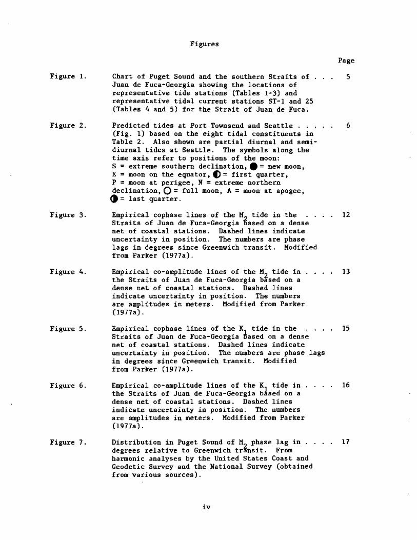
Figure 1.

Figure 2.

Figure 3.

Figure 4.

Figures

Page

Chart of Puget Sound and the southern Straits of . .. 5Juan de Fuca-Georgia showing the locations ofrepresentative tide stations (Tables 1-3) andrepresentative tidal current stations ST-l and 25(Tables 4 and 5) for the Strait of Juan de Fuca.

Predicted tides at Port Townsend and Seattle . . 6(Fig. 1) based on the eight tidal constituents inTable 2. Also shown are partial diurnal and semi-diurnal tides at Seattle. The symbols along thetime axis refer to positions of the moon:S = extreme southern declination, • = new moon,E = moon on the equator, t> = first quarter,P =moon at perigee, N =extreme northerndeclination, 0::: full moon, A = moon at apogee,() = last quarter.

Empirical cophase lines of the M tide in the . 12Straits of Juan de Fuca-Georgia ~ased on a densenet of coastal stations. Dashed lines indicateuncertainty in position. The numbers are phaselags in degrees since Greenwich transit. Modifiedfrom Parker (1977a).

Empirical co-amplitude lines of the M2 tide in . . .. 13the Straits of Juan de Fuca-Georgia based on adense net of coastal stations. Dashed linesindicate uncertainty in position. The numbersare amplitudes in meters. Modified from Parker(1977a) .

Figure 5.

Figure 6.

Figure 7.

Empirical cophase lines of the K1

tide in the . . . •Straits of Juan de Fuca-Georgia oased on a densenet of coastal stations. Dashed lines indicateuncertainty in position. The numbers are phase lagsin degrees since Greenwich transit. Modifiedfrom Parker (1977a).

Empirical co-amplitude lines of the K tide inthe Straits of Juan de Fuca-Georgia bAsed on adense net of coastal stations. Dashed linesindicate uncertainty in position. The numbersare amplitudes in meters. Modified from Parker(1917a) .

Distribution in Puget Sound of M2 phase lag in . .degrees relative to Greenwich transit. Fromharmonic analyses by the United States Coast andGeodetic Survey and the National Survey (obtainedfrom various sources).

iv

15

16

17

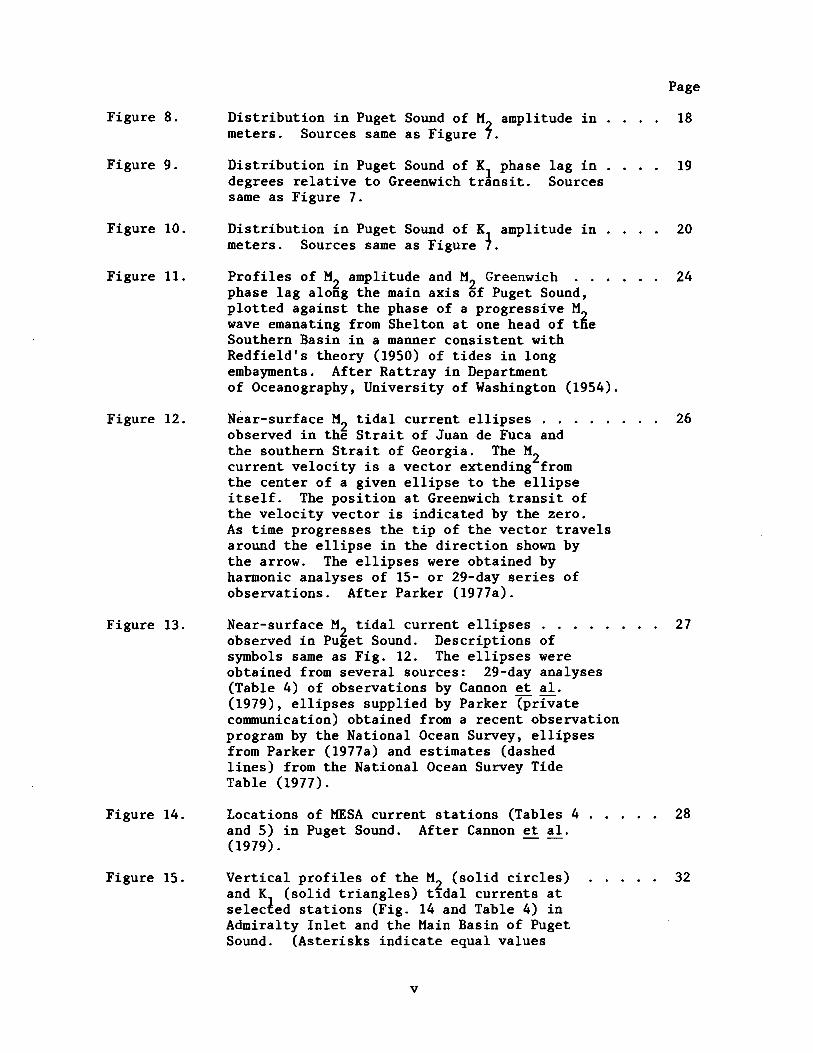
Figure 8.

Figure 9.

Figure 10.

Distribution in Puget Sound of M2 amplitude inmeters. Sources same as Figure 7.

Distribution in Puget Sound of K1

phase lag in .degrees relative to Greenwich transit. Sourcessame as Figure 7.

Distribution in Puget Sound of K1

amplitude inmeters. Sources same as Figure 7.

Page

18

19

20

Figure 11.

Figure 12.

Figure 13.

Profiles of M2 amplitude and M2

Greenwich . . . . 24phase lag along the main axis of Puget Sound,plotted against the phase of a progressive Mwave emanating from Shelton at one head of t~eSouthern Basin in a manner consistent withRedfield's theory (1950) of tides in longembayments. After Rattray in Departmentof Oceanography, University of Washington (1954).

Near-surface M2

tidal current ellipses . . . 26observed in the Strait of Juan de Fuca andthe southern Strait of Georgia. The M2current velocity is a vector extending fromthe center of a given ellipse to the ellipseitself. The position at Greenwich transit ofthe velocity vector is indicated by the zero.As time progresses the tip of the vector travelsaround the ellipse in the direction shown bythe arrow. The ellipses were obtained byharmonic analyses of 15- or 29-day series ofobservations. After Parker (1977a).

Near-surface M2

tidal current ellipses . . • . . 27observed in Puget Sound. Descriptions ofsymbols same as Fig. 12. The ellipses wereobtained from several sources: 29-day analyses(Table 4) of observations by Cannon et al.(1979), ellipses supplied by Parker (privatecommunication) obtained from a recent observationprogram by the National Ocean Survey, ellipsesfrom Parker (1977a) and estimates (dashedlines) from the National Ocean Survey TideTable (1977).

Figure 14.

Figure 15.

Locations of MESA current stations (Tables 4and 5) in Puget Sound. After Cannon et al.(1979).

Vertical profiles of the M2

(solid circles)and K

1(solid triangles) t1dal currents at

seleceed stations (Fig. 14 and Table 4) inAdmiralty Inlet and the Main Basin of PugetSound. (Asterisks indicate equal values

v

28

32

34Figure 16.

Figure 17.

Page

for M2 and K1). Shown are the amplitudes,Greenwich phase lags and flood (toward theSouthern Basin) direction. Values are from29-day harmonic analyses of observationsby Cannon et al. (1979).

Predicted tidal currents (major component) .and excursions at MESA 10 in Admiralty Inletand MESA 2 in The Narrows (Fig. 14) based onthe eight largest constituents observed atthese stations. The symbols along the timeaxis are defined in the caption of Figure 2.

M2 transports (km3) across sections leading to . . . . 39tfie eastern Strait of Juan de Fuca defined asthe water transported across a given sectionduring the one flood interval of the M2 tidalcycle. The tidal prism in the eastern Straitof Juan de Fuca is assumed to be negligible.After Parker (1977a).

vi

Tables

Page

Table 1. General tidal characteristics 1 at selected tide. . . 7stations in the Puget Sound Region (Fig. 1) computedfrom the harmonic constants in Table 2.

Table 2. Tidal harmonic constants for selected tide stations . . 8in the Strait of Juan de Fuca and Puget Sound. Phaselags GO are relative to Greenwich transit. Values fromvarious sources published by the United States Coastand Geodetic Survey and the National Ocean Survey.

Table 3. Ratio of amplitude for the major tidal constituents 9for selected stations in the Strait of Juan de Fucaand Puget Sound computed from the harmonic constantsin Table 2.

Table 4.

Table 5.

Table 6.

Table 7.

Current harmonic constants at selected stations . .(see Figs. 1 and 14 and Table 5) computed by 29-dayharmonic analyses of current observations.

Tidal characteristics and amplitude ratios for themajor components of tidal current constituents atselected stations (see Figs. 1 and 14). Values arederived from current harmonic constants in Table 4.

Tidal excursions 1 and their Greenwich lag2 forselected current stations (see Figs. 1 and 14) inthe Puget Sound region. Values are derived fromcurrent harmonic constants in Table 5.

Tidal prism (volume between mean high water and .mean lower low water) of Puget Sound. Estimatesby Rattray in the Department of Oceanography,University of Washington (1954).

vii

29

30

36

37

amplitude

apogee

apogean range

declination

diurnal

diurnal age

diurnal inequality

ebb

epoch

equilibriumtide

equinox

flood

fortnightly

Greenwich phaselag

Greenwich transit

harmonic analysis

high water

internal seiche

internal wave

isobath

low water

Glossary

maximum of a tidal constituent's tide or tidal current

condition when the moon is at its farthest distance fromthe earth

semidiurnal range at apogee

a~gular distance north or south of the equator

occuring once a day

time elapsed from maximum diurnal forcing until themaximum diurnal tides

difference in successive low water - high water rangeson a given day

motion toward the entrance to the ocean

period of repetition (18.6 years) for long-term variationsin the lunar tides

hypothetical tide that would occur if the oceanresponded instantly to tidal forcing

condition when the sun is directly above the equator

motion away from the entrance to the ocean

occuring every two weeks

time (in units of degrees) elapsed from Greenwich transitof a tidal constituent until its high water (or maximumflood current)

passage over the Greenwich meridian and phase referencefor tidal constituents

method for estimating harmonic constants from time-seriesbased on the sinusoidal nature of the tidal constituents

temporary maximum in height of the sea surface

standing internal wave

wave propagating in the interior of the water driven bythe interior mass distribution

line of constant water depth

principal diurnal declinational (luni-solar) tide

temporary minimum in the height of the sea surface

viii

lunitidal interval time elapsed from Greenwich transit until high water ofthe M2 tidal constituent

M2 principal semidiurnal lunar constituent

major amplitude highest strength of a tidal constituent's current

mean high water average of the high waters (usually two-occurring eachday) over a 19 year period

mean higher highwater

mean lower lowwater

mean range

mean sea level

minor amplitude

mixed-diurnal

mixed-semidiurnal

neap

node

parallax age

perigee

perigean range

phase age

precession

averages of the highest waters occurring each day over a19 year period

average of the lowest waters occurring each day over a19 year period

average vertical displacement between low and high water

average height of sea level over a 19 year period

minimum strength of a tidal constituent's current

occurring primarily once a day but with significantsemidiurnal variations, especially when the moon is nearthe equator

occurring primarily twice a day with 2 distinctdifferences between successive high or low waters

larger semidiurnal lunar elliptic constituent

occurring during quarter moon (moon and sun inquadrature)

location where the tide of a tidal constituent has zero(or very small) amplitude

principal diurnal lunar constituent

time elapsed from lunar perigee until the maximumsemidiurnal lunar tide

condition when the moon is at its closest approach tothe earth

semidiurnal range at perigee

time elapsed from full (or new) moon until the maximumsemidiurnal tides

slow movement of the moon's orbital ellipse causinglong-term (18.6 year period) variations in the lunartides

ix

range

semidiurnal

sequence of tide

solstice

spring

spring-neap

standing wave

tide

tidal constituent

tidal current

tidal curve

tidal datum plane

tidal eddy

tidal ellipse

tidal exchange

tidal excursion

tidal front

tidal intrusion

tidal prism

tidal transport

vertical displacement between sucessive low and highwaters

principal semidiurnal solar constituent

occurring twice a day

phase relationship between M2

, K1

and 01

responsible forthe shape of tidal time-series wfien the moon is awayfrom the equator

condition when the sun is farthest from the equator(largest declination)

semidiurnal tides or tidal currents at full or new moon

occurring as the moon and sun go in and out of alignment

a non-propagating pattern formed by incident and reflectedwaves

vertical displacement of the sea surface caused by thegravitational attraction of the moon and sun

component of the tidal motion occurring at a given(constant) frequency

rate of horizontal tidal motion

time-series of the tide

horizontal surface defined by an average tidal heightsuch as mean lower low water

small, recirculating motion generated by tidal currents

ellipse formed by the tips of the tidal current arrowsduring one cycle of a tidal constituent

water transferred by tidal motions back and forthbetween separate regions

horizontal displacement caused by the tidal currents

sharp horizontal change in the tidal currents or waterproperties caused by tidal motions

water brought into a region by tidal motions

change in water volume of a region occurring within atidal cycle

volume of water moved past a cross-section by tidalmotions

x

tropic

tropic-equatorial

type of tide

condition when the moon is farthest from the equator(maximum declination)

occurring as the lunar declination varies through itscycle

ratio of the diurnal (K +01) tidal amplitudes to thesemidiurnal tidal amplitudes (M2+S2) indicating the relativeimportance of the diurnal and semiaiurnal tides (ortidal currents)

xi

Tides and Tidal Currents of the Inland Waters

of Western Washington1

Harold O. Mofjeld and Lawrence H. Larsen

ABSTRACT. The tides enter the inland waters of Western Washingtonfrom the Pacific Ocean. They form a pattern of nearly standing waveswith large areas of relatively constant amplitude and phase separatedby channels where both change rapidly. The tides are either mixed­semidiurnal or mixed-diurnal. Usually the tides have nearly equalhigh waters with large differences in the low waters. The diurnalrange decreases from 2.4 m at the western end (Neah Bay) of theStrait of Juan de Fuca to a minimum of 1.9 m at the southern end ofVancouver Island (Victoria, British Columbia) and then increases to4.4 m at the southern end of Puget Sound (Olympia). There is anincrease in phase lag away from the ocean due to tidal dissipation.This dissipation is large compared with inland waters with smoothbottom topography and is concentrated in the rugged channels such asAdmiralty Inlet and Haro Strait with strong tidal currents.

The tidal currents often exceed 1 mls in many channels and the Straitof Juan de Fuca. Weaker currents occur in the main basins and side­embayments. Strong vertical shear occurs over sills but the tidalcurrents are relatively independent of depth in the deeper reaches.The tidal currents are rectilinear and flow parallel to the localchannel or shoreline except at the intersection of several channelswhere broad tidal ellipses can occur. In Admiralty Inlet there aremajor diurnal inequalities in both the flood and ebb currents whilein The Narrows the ebb currents are nearly equal in strength. Thetidal prism of Puget Sound amounts to 4.8% of its total volume.Associated with the tidal currents are numerous eddies, fronts andinternal waves.

1 Contribution number 687 from the NOAA/ERL Pacific Marine EnvironmentalLaboratory, 7600 Sand Point Way NE, Seattle, Washington 98115.

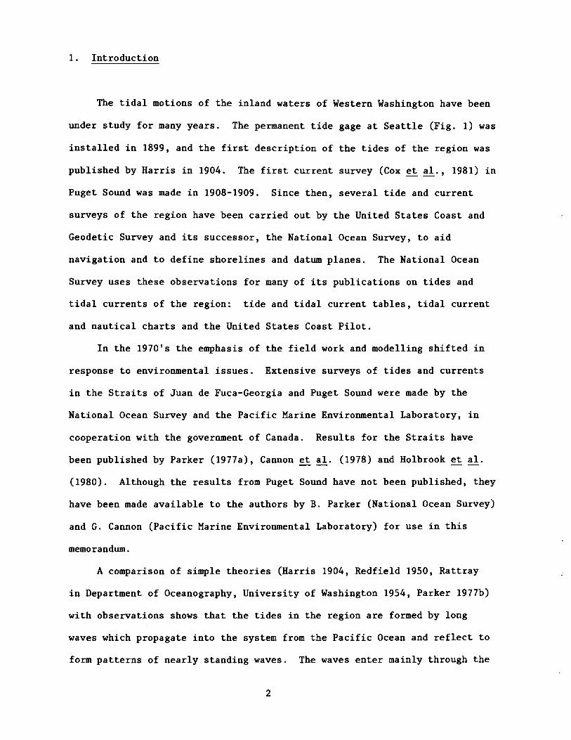
1. Introduction

The tidal motions of the inland waters of Western Washington have been

under study for many years. The permanent tide gage at Seattle (Fig. 1) was

installed in 1899, and the first description of the tides of the region was

published by Harris in 1904. The first current survey (Cox et al., 1981) in

Puget Sound was made in 1908-1909. Since then, several tide and current

surveys of the region have been carried out by the United States Coast and

Geodetic Survey and its successor, the National Ocean Survey, to aid

navigation and to define shorelines and datum planes. The National Ocean

Survey uses these observations for many of its publications on tides and

tidal currents of the region: tide and tidal current tables, tidal current

and nautical charts and the United States Coast Pilot.

In the 1970's the emphasis of the field work and modelling shifted in

response to environmental issues. Extensive surveys of tides and currents

in the Straits of Juan de Fuca-Georgia and Puget Sound were made by the

National Ocean Survey and the Pacific Marine Environmental Laboratory, in

cooperation with the government of Canada. Results for the Straits have

been published by Parker (1977a), Cannon et al. (1978) and Holbrook et al.

(1980). Although the results from Puget Sound have not been published, they

have been made available to the authors by B. Parker (National Ocean Survey)

and G. Cannon (Pacific Marine Environmental Laboratory) for use in this

memorandum.

A comparison of simple theories (Harris 1904, Redfield 1950, Rattray

in Department of Oceanography, University of Washington 1954, Parker 1977b)

with observations shows that the tides in the region are formed by long

waves which propagate into the system from the Pacific Ocean and reflect to

form patterns of nearly standing waves. The waves enter mainly through the

2

Strait of Juan de Fuca with a small contribution through Johnstone Strait at

the northern end of the Strait of Georgia. Partial reflection occurs at

several intermediate locations along the axes of the system (Rattray, in

Department of Oceanography, University of Washington 1954, Parker 1977b,

1980). The tidal motions of the region are subject to unusually strong

dissipation (Redfield 1950) which appears to be concentrated in channels

connecting major basins (Rattray, in Department of Oceanography, University

of Washington 1954, Crean 1969) or near the heads of the system (Parker

1977b, 1980). Over the broad reaches of the Strait of Juan de Fuca, the

earth's rotation causes significant variations in the tides across the

strait (Harris 1904, Parker 1977b). Non-linear effects are also important

(Crean 1969).

The tidal currents are generally aligned with the direction of the

local channel. Their phases relative to the tides' are consistent with

standing waves subject to friction (Bauer 1928). The tidal currents have a

great deal of fine structure that requires detailed modelling to simulate.

Numerous eddies, internal waves and fronts are generated by the tidal

currents. Vertically-averaged models (Crean 1978, Jamart and Winter 1978)

have been developed to study these features in limited locations within the

region. There are also multi-level models (Crean, private communication)

under development to study the vertical structure of the tidal currents.

In this memorandum we shall summarize what is known about the tides and

tidal currents of the region as seen from observations and numerical models.

The region of interest includes the Strait of Juan de Fuca and the southern

Strait of Georgia as well as Puget Sound. This is because the tidal motions

in the straits drive those in Puget Sound to form a unified, co-oscillating

system. There are also many similarities in the tidal dynamics of Puget

Sound and the straits, and the insights gained from studying the tidal

3

motions in the straits are useful in understanding those in Puget Sound.

Enough is known about the tides and tidal currents of the combined system to

provide a general description of the tidal motions and to identify many of

the processes that control these motions. However, the region is so complex

that the details of the tidal distributions and the tidal dynamics remain to

be worked out.

2. Tides

2.1 Patterns of Tidal Curves

Both the diurnal and semidiurnal tides are important in the region

(Fig. 1). Typical tidal curves (Fig. 2) are either mixed-diurnal or mixed­

semidiurnal in type. Tidal ranges (Table 1) are several meters with the

maximum diurnal range (4.4 m) in the southern-most reaches of Puget Sound

(Olympia). The phase relationship between the diurnal and semidiurnal tides

(sequence of tide around 180°) causes nearly equal high waters but produces

a large inequality in the low waters, except during the short time when the

moon is near the equator (Fig. 2). The influence of the diurnal tide is

particularly strong in the eastern Strait of Juan de Fuca (Victoria) where

the semidiurnal (mean) range is a minimum.

The fortnightly variations in range are due primarily to the tropic­

equatorial modulations in the diurnal tides. This is because the diurnal

tides are relatively strong in the region and because the semidiurnal solar

tide S2 is relatively small (Tables 2 and 3), producing only a modest

spring-neap modulation in the semidiurnal tides. Figure (2) shows that the

monthly modulations in the semidiurnal tide are comparable with the

4

125°W 124° 123° 122°490N I I I I 490NI .~ v VI: t=.\ _6 I

VI48°

47° Olympia

48°

47°

125°W 124° 123° 122°

Figure 1. Chart of Puget Sound and the southern Straits of Juan de Fuca-Georgia showing the locationsof representative tide stations (Tables 1-3) and representative tidal current stations ST-land 25 (Tables 4 and 5) for the Strait of Juan de Fuca.

0\

Figure 2.

TIDE AT PORT TOWNSEND (48°08N, 122°46W)

TIDE AT SEATTLE (47° 37 N, 122° 20W

PARTIAL DIURNAL TIDE AT SEATTLE

PARTIAL SEMIDIURNAL TIDE AT SEATTLE

S. E() P N 0 E A<I S. EPr--__u II I I I I" I I "I 1 I I I 1 I I II 6 II 16 2 I 26 31 5 10

JAN 81 FEB 81

Predicted tides at Port Townsend and Seattle (Fig. 1) based on the eight tidal constituentsin Table 2. Also shown ,are partial diurnal and semidiurnal tides at Seattle. The symbolsalong the time axis refer to positions of the moon: S = extreme southern declination,tt= new moon, E = moon on the equator,tD= first quarter, P = moon at perigee, N = extremenorthern declination,()= full moon, A = moon at apogee,(t= last quarter.

Table 1. General tidal characteristics l at selected tide stations in thePuget Sound Region (Fig. 1) computed from the harmonic constantsin Table 2.

PortSTATION Neah Bay Victoria Townsend Seattle Olympia

Kl+OlType of tide -- 0.79 2. 10 1.44 0.97 0.75

M2 +S2

Sequence of tide M~-K~-O~ 126 159 190 198 199

Range (m)2

Mean 1.7 (0.8) 1.6 2.3 3.22

Diurnal 2.4 1.9 2.6 3.4 4.4

Spring 2.1(M2 +S2) 2. 1 1.0 ' 1.8 2.8 3.8

Neap 2.1(M2-S2) 1.2 0.6 1.1 1.7 2.3

Perigean 2.2(M2+N2) 2. 1 1.0 1.8 2.8 3.8

Apogean 2.2 M2-1. 7 N2 1.4 0.7 1.2 2.0 2.7

Interval (h)

Lunitida1 M~/28.98 8.5 10.9 12. 1 12.8 13.5

Phase age 0.984(S~-M~) 27 17 24 27 33

Parallax age 1.837(M~-N~) 42 57 55 57 50

Diurnal age 0.911(K~-OV 15 20 19 20 21

12formu1as derived by Zet1er (1959).values taken from tide tables (National Ocean Survey 1979)

7

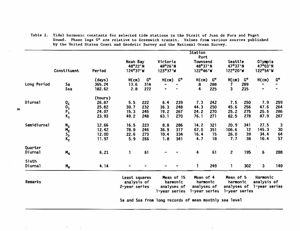
Table 2. Tidal harmonic constants for selected tide stations in the Strait of Juan de Fuca and PugetSound. Phase lags GO are relative to Greenwich transit. Values from various sources publishedby the United States Coast and Geodetic Survey and the National Ocean Survey.

long Period

Constituent

SaSsa

Period

(days)365.24182.62

Neah Bay48°22 ' N

124°37'W

H(cm) GO13.6 3142.8 272

Victoria48°26 ' N

123°37'W

H(cm) GO

StationPort

Townsend48°37 ' N

122°46'W

H(cm) GO8 2884 225

Seattle47°37 ' N

122°20 ' W

H(cm) GO7 2893 215

Olympia47°03'N

122°54'W

H(cm) GO

7.9 25947.6 26425.5 28687.9 287

00

Diurnal

Semidiurna1

Q101P1K1

NzMzSzKz

(hours)26.8725.8224.0723.93

12.6612.4212.0011.97

5.5 22230.7 23215.3 24549.2 248

16.5 22378.0 24622.6 2735.9 266

6.4 23936.3 24819.2 26763.1 270

8.8 28636.9 31710.4 3341.8 341

7.3 24244.3 25024.2 27076. 1 271

14.2 32167.0 35116.4 154.7 18

7.5 25045.6 25625.2 27582.5 278

20.9 341106.6 1226.0 397.7 38

27.5145.334.410.4

3306457

QuarterDiurnal

SixthDi urna1

M4

Ms

6.21

4. 14

61 4

1

61

249

2

1

195

302

6

3

288

140

Remarksleast squaresanalysis of

2-year series

Mean of 15harmonic

analyses of1-year series

Mean of 4harmonic

analyses of1-year series

Mean of 5 Harmonicharmonic analysis of

analyses of 1-year series1-year series

Sa and Ssa from long records of mean monthly sea level

Table 3. Ratio of amplitude for the major tidal constituents for selectedstations in the Strait of Juan de Fuca and Puget Sound computedfrom the harmonic constants in Table 2.

STATION

TidalConstituents Equilibrium Neah Bay Victoria Port Townsend Seattle Olympia

Diurnal

Semidiurna1

N2/M2

S2 /M2

K2 /S2

0.19

0.71

0.33

0.19

0.47

0.27

0.18

0.62

0.31

0.21

0.29

0.26

9

0.18

0.58

0.30

0.24

0.28

0.17

0.16

0.58

0.32

0.21

0.24

0.29

0.16

0.55

0.31

0.20

0.24

0.30

0.17

0.54

0.29

0.19

0.24

0.30

fortnightly modulations. This can also be seen from semidiurnal amplitudes

(Tables 2 and 3): N2 (associated with the monthly modulation) is n~arly as

large as S2 (associated with the fortnightly modulation). Both semidiurnal

modulations lag in time their equilibrium counterparts. For the fortnightly

modulation of S2 and M2 the corresponding phase age (Table 1) increases from

23 hours at the entrance (Port Townsend) to Puget Sound to 33 hours at the

southern end (Olympia). On the other hand, the parallax age associated with

the monthly modulation (N2 and M2) does not show a trend; in Puget Sound,

the average parallax age is 54 hours. The diurnal age (01 and K1) is about

20 hours.

There is a seasonal relationship between spring and tropic tides. As

discussed by Crean (1969), at the solstices (December and June) new and full

moons occur at times of large lunar and solar declinations. The spring and

tropic tides then coincide, giving rise to large tidal ranges and inequali­

ties. At the equinoxes, new and full moons occur when the moon and sun are

near the equator. Then, spring tides have small inequalities and neap tides

have large inequalities. Because of the relationship between the phases of

M2 , K1 , and 01 in the region, the lowest tides occur at night during the

winter and during the day in summer. The tides have variations through the

year because earth's orbit around the sun is inclined (23.5°) relative to

the equator and because the orbit is elliptical.

Over several years the lunar constituents vary periodically due to the

18.6-year precession of the moon's orbit. The harmonic constants (Table 2)

are averages over the precessional period (19 years in practice). The major

effect is due to the declination of the moon which varies from 18.3° to

28.6° and has a significant effect on the amplitudes of 01 (~18%) and K1

(~11%). The larger semidiurnal constituents M2 and N2 are much less

affected (~4% each). It is over the precessional period that the United

10

States Coast and Geodetic Survey (Marmer, 1951) averages tidal heights to

obtain the tidal datum planes. One of these, mean lower low water MLLW is

the reference plane for nautical charts along the west coast of the United

States. By direct averaging over three 19-year epochs (1899-1917), 1915­

1933, 1930-1948) Marmer (1951) found for Seattle that relative to mean lower

low water, the heights of the tidal datums mean higher high water and mean

sea level were 3.192, 3.189, 3.199 m and 2.023, 2.018, 2.025 m, respectively.

Discussions of seasonal and longer period variations and trends in sea level

are given by Marmer (1951), Waldichuk (1964), and Hicks (1973).

2.2 Geographical Distributions of the Tides

The geographical distributions of the semidiurnal and diurnal tides can

be represented by the largest constituent of each species since the ratios

of constituents (Table 3) remain relatively constant over the region.

Typical of the semidiurnal tides, the M2 tide varies considerably within the

region. Following the changes in M2 phase lag from the entrance of the

Strait of Juan de Fuca, the MZ phase (Fig. 3) increases eastward through the

western Strait of Juan de Fuca and more rapidly in the eastern Strait and

the San Juan Archipelago. In the Strait of Georgia, the northward increase

in MZ phase is small particularly in the northern reaches. The total

increase in M2 phase through the Staits of Juan de Fuca - Georgia is about

148°. The MZ amplitude (Fig. 4) decreases dramatically from the entrance to

a minimum at the southern end of Vancouver Island. After increasing rapidly

through the San Juan Archipelago, the MZ amplitude increases more gradually

in the southern Strait of Georgia and is nearly constant over the northern

reaches of the system where the M2 amplitude is slightly larger (1.3x ) than

its value at the entrance to the Strait of Juan de Fuca.

11

126°W 125° 124° 123° 122°

49°

SOON

'OJ E·' ....·., """ct'· t- 480

122°

~." t·:'#' ,.:. 3520

123°

PHASE LAG (GO)

124°1250

II

I/2370

//

126°W

49°

48 0 I V ""Yo- -:·;U,"'liii i

SOON

~

N

Figure 3. Empirical cophase lines of the M tide in the Straits of Juan de Fuca-Georgia based on adense net of coastal stations. bashed lines indicate uncertainty in position. The numbersare phase lags in degrees since Greenwich transit. Modified from Parker (1977a).

126°W 1250 1240 1230 1220

....w

500 N

490

I\

.94\\\

(\

.91\\\

AMPLITUDE (m) 500 N

490

123012401250126°W

480 I I I v· I ···..·l':···:llYt:,\ tf '!"::"'~ "'22:;:' ~480

1220

Figure 4. Empirical co-amplitude lines of the M2 tide in the Straits of Juan de Fuca-Georgia based ona dense net of coastal stations. Daslied lines indicate uncertainty in position. Thenumbers are amplitudes in meters. Modified from Parker (1977a).

Like the other diurnal tides, the K1 tide increases continuously in

phase lag and amplitude through the system. In the Straits of Juan de

Fuca - Georgia (Figs. 5 and 6) the largest increases in phase and amplitude

occur in the western Strait of Juan de Fuca and through the San Juan

Archipelago. The total changes in K1 through the overall system are 39° in

phase and a factor of 2.0 in amplitude. According to Redfield (1950) both

the incident H2 (4.83 hrs) and K1 (4.92 hrs) waves take about 5 hours to

propagate from Clayoquot on the Pacific Coast to Whaleton in northern Strait

of Georgia. Each slows down on entering the Strait of Juan de Fuca, each

proceeds at 18 mls (35 knots) between Port Angeles and Point Atkinson,

British Columbia, and then speeds up dramatically in upper Strait of

Georgia. Redfield noted that relative to the K1 wave the H2 wave undergoes

a delay of about \ hour in the intermediate channels of the system.

In Puget Sound (Fig. 7 and 8) the H2 phase and amplitude increase

toward the heads of the system; they increase most rapidly through Admiralty

Inlet and The Narrows and are relatively constant in the major basins. The

total H2

phase increase (Table 2) in Puget Sound is 39°. There are also

large phase increases in the narrow channels connecting two small basins,

Dyes Inlet and Oakland Bay, with the main system. Along the main axis of

Puget Sound, the H2

amplitude increases by a factor of 2.2 from the northern

end of Admiralty Inlet (Port Townsend) to the southern end of the southern

basin (Olympia). In Puget Sound (Table 2, Figs. 9 and 10) the total

increase in K1 phase (16°) and amplitude (1.2x ) are relatively small.

Tidal Dynamics

There are a number of theoretical models which provide considerable

insight into the tidal behavior of the region. While many of the details

remain to be worked out, the important processes controlling the tides

14

126°W 125° 124° 123° 122°

~

V1

500 N

49° \\\

2400\

\\

PHASE LAG (GO)

~281°

~750. ; .. , ':::" 0

,""~ "'~270;.:. ~.: .... 2690

,,' :;", <:: 2680

'. ," ~269°

~270°»c~C273°

500 N

49°

123°124°125°126°W

48° I I I y. I ':l ::;}\,.i\1ti 1;,,:'<"'0 Ya':.' r48°

122°

Figure 5. Empirical cophase lines of the K tide in the Straits of Juan de Fuca-Georgia based on adense net of coastal stations. ~ashed lines indicate uncertainty in position. The numbersare phase lags in degrees since Greenwich transit. Modified from Parker (1977a).

.....C7'

500 N

490

126°W

126°W

1250

1250

1240

1240

1230

1230

\(i7A;,:76

1220

500 N

490

Figure 6. Empirical co-amplitude lines of the K1

tide in the Straits of Juan de Fuca-Georgia based ona dense net of coastal stations. Dasfied lines indicate uncertainty in position. Thenumbers are amplitudes in meters. Modified from Parker (1977a).

I 51

301

I 51

151

15'

451

451

301

301

151

151

151

45'

301

151

Figure 7. Distribution in Puget Sound of M2

phase lag in degrees relative toGreenwich transit. From harmonic analyses by the United StatesCoast and Geodetic Survey and the National Survey (obtained fromvarious sources).

17

1 51

451

30'

151

1 51

M2 AMPLITUDE(m)

15'

451

451

301

301

151

15'

151

451

301

151

Figure 8. Distribution in Puget Sound of M2 amplitude in meters. Sourcessame as Figure 7.

18

15'

151

301

301

451

151

15'

K1 PHASE LAG(oG)

151

151

151 15'

301 30'

451

451

Figure 9. Distribution in Puget Sound of K1

phase lag in degrees relative toGreenwich transit. Sources same as Figure 7.

19

I S\

4S\

30'

I SI

lSi

K1 AMPLITUDE(m)

lSi

4S1

451

30'

30'

IS'

lSi

lSi

4S1

30'

Figure 10. Distribution in Puget Sound of KI

amplitude in meters.Sources same as Figure 7.

20

appear to be identified. The tidal distributions in the Straits of Juan de

Fuca - Georgia and Puget Sound indicate that the tides are long waves

propagating in from the Pacific Ocean and forming standing wave patterns

through the combination of incident and reflected waves (Harris 1904, Bauer

1928, Redfield 1950, Rattray in Department of Oceanography, University of

Washington 1954, Parker 1980).

The large areas of relatively constant phase and large amplitude are

found near reflecting boundaries. These areas include the northern reaches

of the Strait of Georgia (Figs. 3 - 6), Southern Basin of Puget Sound

(Figs. 7 - 10), Whidbey Basin and Hood Canal. Similar regions in the

eastern Strait of Juan de Fuca and the Main Basin of Puget Sound indicate

that partial reflection is occurring at intermediate locations along the

main channels. The minimum in the M2 amplitude (Fig. 4) in the eastern

Strait of Juan de Fuca is a node formed by the destructive interference of

incident and reflected waves. It is located about 1/4 wavelength from the

primary reflecting boundary at the northern end of the Strait of Georgia.

Because the system is shorter than 1/4 wavelength for the K1 tide, there is

no K1

node and the K1

tide therefore increases continuously in amplitude

(Fig. 6) from the entrance.

The increase in phase lag with distance into the system is due to

frictional dissipation and wave scattering. A bulk estimate (Redfield 1950)

of the dissipation can be obtained by fitting the distribution of M2 and K1

tides to frictionally damped waves. The fit shows that the dissipation

averaged over the Straits of Juan de Fuca - Georgia is significantly greater

than in either Long Island Sound or the Bay of Fundy. Crean (1969) finds

that a best fit of a coarsely segmented model to observations requires a

bottom drag coefficient in the rugged San Juan Archipelago that is an order

of magnitude (0.02 to 0.03) larger than generally accepted values (0.002 to

21

0.004) for open regions with smooth bottoms. Non-linear interactions

between tidal constituents (due to the high dissipation in the San Juan

Archipelago) are needed to explain the K1 amplitude in the Strait of Georgia

(Crean 1969): Without the non-linear interactions, the K1 amplitude in the

Strait of Georgia would be -10 cm too small. By fitting a one-dimensional

model to observations, Parker (1980) finds that theM2 tide looses 17% of

its amplitude when propagating through the San Juan Archipelago and looses

an additional 18% on reflecting at the northern end of the Strait of

Georgia. The M2 tide also looses continuously 53% of its amplitude per

wavelength along its path of propagation due to frictional dissipation and

wave-scattering. The K1 tide suffers comparable losses of amplitude (Parker

1980) in the San Juan Archipelago and northern Strait of Georgia, but its

continuous decay is much less (10% per wavelength) because the K1 currents

are much less than the M2 currents and its wavelength is twice as long.

The Straits of Juan de Fuca - Georgia are wide enough to allow major

cross-channel variations in the tides. The minimum in M2 amplitude (Fig. 4)

is located on the northern side of the Strait of Juan de Fuca. Explana­

tions for this (Parker 1977b) rely on the effect of the earth's rotation and

the influence of Puget Sound: Let us assume that the incident and reflected

M2 waves are damped Kelvin waves with higher amplitude on the right side of

the channel, looking in the direction of propagation. At a given cross­

section, the amplitude of the reflected wave is smaller than that of the

incident wave because of the reflected wave has been attenuated over the

path from the cross-section to the reflecting boundary (primarily the

northern end of the Strait of Georgia) and back again. As observed the

largest M2 amplitudes should then be along the southern shore of the Strait

of Juan de Fuca. The minimum M2 amplitude is on the northern shore because

of sufficient dissipation (Parker 1977b) while the relatively large M2

22

amplitudes near the northern end of Admiralty Inlet are due to the co­

oscillation with Puget Sound. Harris (1904) associates the influence of the

earth's rotation with the crowding of cophase lines on the northern side of

the Strait of Juan de Fuca and their spreading on the southern side.

In Admiralty Inlet and The Narrows the large changes of M2 phase

(Fig. 11) are caused by frictional dissipation (Rattray in Department of

Oceanography, University of Washington 1954). Friction is also responsible

for the large M2 phase change along the shallow Hammersley Inlet (between

Shelton and Arcadia) off the Southern Basin. The change in M2 amplitude

(Fig. 11) between Seattle and the southern end of Admiralty Inlet is

probably due to the influence of the Whidbey Basin which increa$es the

effective length of the Main Basin as seen by the tides (Rattray in

Department of Oceanography, Univeristy of Washington 1954). The channels

and basins of Puget Sound are too narrow to allow large cross-channel

variations in the tides.

3. Tidal Currents

Strong tidal currents are common in Puget Sound and the Straits of Juan

de Fuca-Georgia; current speeds over 1 mls can be found in many channels.

Weaker tidal currents are prevalent in the deeper reaches while the tidal

currents are barely detectable in many side-embayments and blind arms. The

transitions in current speeds between these flow regimes are often abrupt

and this produces strong tidal fronts. The flow of strong tidal currents

past points of land generates eddies which wander through the system.

These secondary features associated with the tidal currents are discussed in

the next section. In the present section, we shall smooth over secondary

23

M2 AMPLITUDE (m)

po (J'1 0

SheIton ----.-"""T'"-...,.....-r_~-_r_-.,...____,-""T""-r____,r__.-...,.__,r__on

~o3

;:, 3-C'I>C'I> ~-(/I

Ci"'<

Arcadia

CJ)CDOo c:(/I -_. ':::T

-f;:'~':::T ;:,C'I>

Z0-----.......oE(/I

Dofflemyer

HendersonInlet

Hyde PointlStei lacoomJ-

S. End Narrows

Gig HarborI I Tacomal

Ou t rmaster Hbrj-Des Moines

ColbySeattle

-J(}l

o

-c:Q. Q.

C'I>-- 0C'I>... -C'I>3:;:,

n NC'I>

o N ~ (1)000

DIFFERENCE IN M2 PHASE LAGG(SHELTON)-G IN DEGREES

Figure 11. Profiles of M2 amplitude and M2 Greenwich phase lag along themain axis of Puget Sound, plotted against the phase of aprogressive M2 wave emanating from Shelton at one head of theSouthern Basin in a manner consistent with Redfield's theory(1950) of tides in long embayments. After Rattray in Departmentof Oceanography, University of Washington (1954).

24

features and focus on the general characteristics of the tidal currents in

the region.

3.1 Geographical Distributions of Tidal Currents

In general, tidal currents of the region vary with depth as well as

location. As we shall see, current speeds decrease with depth due to bottom

drag and the directions of the currents are relatively independent of depth;

coupling to internal waves may also influence the vertical structure of the

tidal currents. Each tidal constituent forms a pattern of tidal ellipses;

shown in Figures 12 and 13 are the near-surface tidal ellipses for the

strongest current constituent M2 . Like the other constituents (Table 4),

the M2 ellipses are narrow and aligned with either the local direction of

the channel or a nearby shoreline. The motion is rectilinear in many

locations, but broad ellipses do occur (Figs. 12 and 13) where several

channels meet.

Strong tidal currents (Fig. 13 and Table 4) occur in Admiralty Inlet

and The Narrows. The strongest currents (>4 m/s) in the region flow through

Deception Pass in response to large differences in tidal heights (primarily

semidiurnal) between the eastern Strait of Juan de Fuca and northern end of

the Whidbey Basin. Weak tidal currents prevail in the parts of the Whidbey

Basin and Hood Canal that are away from their entrances. Although the

Southern Basin occupies one head of the Puget Sound system, strong tidal

currents (Fig. 13) occur in all the narrow channels connecting its network

of sub-basins. The Strait of Juan de Fuca (Fig. 12 and Table 4) is swept by

strong tidal currents. Particularly intense tidal currents (Fig. 12) occur

in the straits and channels through the San Juan Archipelago because of the

strong co-oscillation between the Straits of Juan de Fuca and Georgia.

25

30' 151124°W 45' 30' 15' 1230 45' 30'

45'

15'

30'

a 100 200 300I , I !

cm/s

4 5 6

3~ Ie: ~9-J 12 .. 10

M2 TIDAL CURRENTS

151

30'

451

490 N , I I "';",.::.1' Ii." • ,,1:: ' 'l' .,\ I .J.: I I 49°N

N0\

30' 15' 124°W 45' 30' 15' 1230 45' 301

Figure 12. Near-surface M2

tidal current ellipses observed in the Strait of Juan de Fuca and the southernStrait of Georgia. The M

2current velocity is a vector extending from the center of a given

ellipse to the ellipse itself. The position at Greenwich transit of the velocity vector isindicated by the zero. As time progresses the tip of the vector travels around the ellipse inthe direction shown by the arrow. The ellipses were obtained by harmonic analyses of 15- or29-day series of observations. After Parker (1977a).

45'

30'

IS'

300,

cm/s100 200o

IS' 123°W 4S' 30' IS'

,l.,,. (:)

."

..--.~

IS' IS'

.-...

M2 TIDAL CURRENTS

IS'

45'

30'

IS'30'4S'

_, ---,, =--__--, ,-- ,-_--.J

IS' 12YW

Figure 13. Near-surface M tidal current ellipses observed in Puget Sound.Descriptions o~ symbols same as Fig. 12. The ellipses wereobtained from several sources: 29-day analyses (Table 4) ofobservations by Cannon et a1. (1979), ellipses supplied by Parker(private communication) obtained from a recent observation programby the National Ocean Survey, ellipses from Parker (1977a) andestimates (dashed lines) from the National Ocean Survey TideTable (1977).

27

4S1

301

lSi

':'.0.

4S'

4S1

12~30'W

lSi

lSi

4S'

30'

IS'

Figure 14. Locations of MESA current stations (Tables 4 and 5) in PugetSound. After Cannon et al. (1979).

28

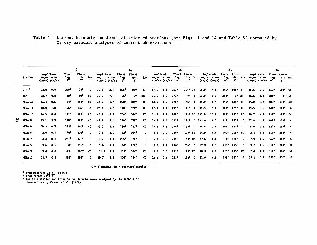
Table 4. Current harmonic constants at selected stations (see Figs. 1 and 14 and Table 5) computed by29-day harmonic analyses of current observations.

StationAllplitude

.ajor .inor(cals) (cll/s)

Floodlag

GO

01

Flooddir

TORot.

Allplitude Flood..jor .inor lag(cals) (cll/s) GO

IIIFlood

dir.TO

Rot.Allplitude

..jor _iDor(CII/a) (CII/a)

HzFlood

181GO

Flood Allplitudedir. Rot. aajor .inor

TO (0./0) (0./0)

"zFlood Flood

181 dir.GO TO

Sz

Allplitude Flood FloodRot. aajor .inor 101 dir. Rot.

(CII/a) (0./0) GO TO

305° CC

930 C

180 CC

1440 CC

163° CC

182° CC

1400 CC

7.0 1.1 3140 2890 CC

3.2 0.5 3110 2420 C

7.9 0.4 3490 1830 C

3.4 0.8 3170 2120 CC

15.6 1.6 3100 1180 CC

16.6 2.3 321 0 10 CC

19.5 1.1 3020 1690 C

25.2 1.2 3280 1310 CC

2890 1520 C 19.1 0.2 3210 1530 C

2900 2430 C

2760 2950 CC

3140 1820 C

2980 1300 C 25.0 1.2 3240 1340 C

2970 2000 CC

2860 1720 C 27.8 1.8 3080 1740 C

2980 1700 CC 28.7 4.7 3250 1720 CC

299 0 00 CC

2800 1730 C

3050 1060 C

2940 1350 C

0.9

0.7

2.7

0.9

4.0

7.5

3.2

5.7

1.8

0.6

0.6

90 C 67.0

1520 C 81.9

1710 C 87.5

1980 CC 14.9

2360 C 12.9

1320 C 89.7

1830 CC 27.6

1320 C 96.4

2890 CC 28.9

1260 CC S8.9

1750 CC 101.8 13.0

1750 C 102.4

2.6 0.9 2690

5.8 0.5 2920

2.5 1.1 2780

4.6 0.0 2510

18.3 1.5 2700

15.3 0.5 2630

22.6 1.9 257 0

20.5 2.6 2720

17.0 1.0 257 0

21.3 4.1 2680

21.1 3.6 2710

16.1 1.5 2530

C

C

CC

CC

CC

C

C

C

CC

CC

98° C

7° CC

190° 178°

1940 132°

1920 2040

235° 174°

194° 224°

151° 304°

170° 154°

173° 174°

204° 164°

200° 134°

2060

196°

0.2

2.4

7.1

4.7

4.2

6.6

2. 1

2.1

0.6

0.3

0.4

29.7

11.9 1.8

38.6

38.8

34.5

28.4

45.6

41.6

39.0

7.5

10.7

5.4

C

C

C

C

C

155°

1960

1700

219°

1860

158°

184°

162°

170°

251°

160°

129°

1360

155°

171 0

200°

1580

23.0 5.5

22.7 4.8

21.4 0.5

13.9 1.8

24.5 6.6

23.1 3.7

19.3 0.7

2.5 0.1

3.4 0.1

3.6 0.5

9.0 0.8

21.7 0.1MESA 2

MESA 3

ST-l 1

25z

MESA 121

MESA 11

MESA 10

~ MESA 9

MESA 8

MESA 6

MESA 7

MESA 5

C =clockwise, cc =counterclockwise

1 fr~ Holbrook et al. (1980)2 fr~ Parker (19778)1 for this station and those below: f~ hanlOnic analyses by the authors of

observations by Cannon et al. (1979).

Table 5. Tidal characteristics and amplitude ratios for the major components of tidal current constituentsat selected stations (see Figs. 1 and 14). Values are derived from current harmonic constants inTable 4.

IntervalsDepth Type of Sequence Hajor axis Luni- Phase Parallax Diurnal

Station Location meter bottom tide of tide current ratios tidal Age Age Age

latitude (m) (m) K1+0 1 H~-KY-OY 01 Nz Sz (h) (h) (h) (h)-- - - -longitude Hz+Sz K1 Hz Hz

480 14.4NST-1 1230 40.8W 10 170 0.83 2590 0.60 0.27 0.26 10.5 4.9 95.5 5.5

480 27.1N25 1230 09.4W 21 132 0.74 305 0 0.59 0.31 0.25 10.3 21.6 51.4 34.6

w 480 08.7N0MESA 12 1220 41.9W 89 10 0.49 2700 0.62 0.23 0.28 10.1 33.5 40.4 14.6

480 01.6NMESA 11 1220 38.9W 51 60 0.40 3120 0.49 0.19 0.22 9.7 21.6 42.3 16.4

480 01.7NMESA 10 1220 38.0W 14 108 0.54 2830 0.54 0.21 0.28 10.3 26.6 55.1 30.1

480 01.8NMESA 9 1220 37.2W 16 112 0.50 2980 0.56 0.22 0.27 9.9 21.6 53.3 29.2

47 0 57.5NMESA 8 1220 34.5W 15 109 0.48 3020 0.49 0.19 0.26 10.3 25.6 51.4 29.2

47 0 42.3NMESA 6 1220 26.6W 20 200 0.55 2950 0.33 0.17 0.23 10.2 19.7 51.4 20.0

470 26.5NMESA 7 1220 31.4W 15 115 0.40 1880 0.32 0.21 0.29 10.8 34.4 40.4 -14.6

470 20.0NMESA 5 1220 26.1W 26 181 0.56 2960 0.67 0.19 0.25 10.0 20.7 22.0 31.0

47 0 19.4NMESA 3 1220 31.8W 19 102 0.58 3560 0.76 0.16 0.24 9.5 37.4 45.9 20.0

47 0 18.4NMESA 2 1220 33.4W 43 73 0.51 3430 0.73 0.19 0.23 10.0 31.5 47.8 31.0

3.2 Vertical Dependence of Tidal Currents

How the tidal currents in Puget Sound (Fig. 14) vary with depth depends

on the speed of the currents and the total depth. In the high-speed regimes

of Admiralty Inlet (Stas. MESA 8 and 10, Fig. 14) observed tidal currents

(Fig. 15) decrease rapidly from the surface with strong shear throughout the

water column. There is also a hint of strong shear from the near-bottom

observations in The Narrows (Sta. MESA 2). The large shear over the water

column shows that there is strong turbulence throughout the water column and

that strong frictional dissipation is occuring. In the Main Basin (Fig. 15)

the tidal current speeds are much less than in Admiralty Inlet and the shear

(though not well-resolved) is confined near the bottom; the tidal current

speeds are essentially independent of depth over most of the water column.

The phase lag of the tidal currents should decrease with depth because

the slower currents nearer the bottom have less inertia to overcome. This

is the case (Fig. 15) in Admiralty Inlet (Stas. MESA 8 and 10), Colvos

Passage (Sta. MESA 7) and The Narrows (Sta. MESA 6). The K1 phase lag at

MESA 6 increases with depth while the M2 phase lag decreases as expected.

Presently, the behavior of K1 phase at Sta. MESA 6 is not understood. The

directions of the currents (Fig. 15) are relatively independent of depth and

essentially the same for diurnal (K1) and semidiurnal (M2) constituents.

The exception is again Sta. MESA 6 where the tidal currents veer westward

with depth.

Holbrook et al. (1980) observe that the tidal currents in the Strait of

Juan de Fuca show significant variation with depth in which the ellipses

near the bottom are smaller and broader than those near the surface. This

is consistent with the results of a seven-level three dimensional numerical

study presently in progress (Crean, private communication). Holbrook et al.

31

.. • .. •.. • .. •50- .. • .. •100 .. • ~)JjJ) »7»"7m

50

MESA 8 (Admiralty Inlet!Amplitude (Major Allis)o 50 100cm/so+-_.L..--...J._--J..._.......

MESA 10 (Admiralty Inlet!

o 50 loocm/s0+--.........- ..'------'-............ ... ... .

Flood Phase Lall200° 3000 G

I !

200° 3000 GI I.. •.. •.. •.. •

~> ';;)7>~k;?

Fload Direction100° 2000 T

I SI I

**..>;;»M'>>>>>>>7

100°I

>w>>>,,;~>y

MESA 6 (Main Basin)

o 50cm/s0+--.1...-----1.

*'50 .....100- ...

200° 3000 G 100° SI2900T

I ! !

~, 'III.. • •.. • .... • ..

150

200-lj-m"7"-'777?m I,. ;;,.>-'>:;>;;~

MESA 7 (Colvos Passage)

0EO50cm/s.. .50 .. •

I~O u~,,·,

200° 3000 G 100° Sl2pooTI I I.. • •.. • -.. • lit

)},»>.... , , >?/?/ ; in;; >?JJ??7;

// /''-*~ >>> >?

Figure 15. Vertical profiles of the M2

(solid circles) and K1

(solidtriangles) tidal currents at selected stations (F1g. 14 andTable 4) in Admiralty Inlet and the Main Basin of Puget Sound.(Asterisks indicate equal values for M2 and K1). Shown are theamplitudes, Greenwich phase lags and flood (toward the SouthernBasin) direction. Values are from 29-day harmonic analyses ofobservations by Cannon et ale (1979).

32

(1980) also find seasonal variations and large irregularities in the cross­

channel currents near the surface that are due probably to the internal

seiching discussed by Crean and Miyake (1976) and Crean (1978). There is

also significant vertical shear in the tidal currents near the surface

(Holbrook and Frisch 1981). The reasons for this shear are not known at

present.

3.3 Patterns of the Tidal Current and Excursion Curves

Like the tides (Fig. 2), the tidal currents (Fig. 16) of the region

contain important contributions from both diurnal and semidiurnal

constituents. However, the patterns of the tidal current curves differ

markedly from those of the tides. The tidal currents (Table 5) are more

semidiurnal (type ~0.5). In Puget Sound, the sequence (M2-Ki-Oi) of the

tidal currents (Table 5) vary from about 280° in Admiralty Inlet to 340° in

The Narrows. Hence, in Admiralty Inlet there often are major diurnal

inequalities in both flood and ebb currents while in The Narrows there often

is a major inequality in the flood currents with the ebb-currents of nearly

equal strength.

For a pure standing wave the tidal current should lead the tide by 90°;

the lead is 0° for a purely progressive wave. The M2 tidal current at Sta.

MESA 6 (Table 4) off Seattle leads the tide (Table 2) at Seattle by 75°;

the K1 lead is 86°. Hence, the phase relationship between the tides and

tidal currents near Seattle shows that the tidal motions are due to standing

waves with some progression.

Besides the tides and tidal currents, a third kind of tidal motion is

the tidal excursion (Table 6). It is the apparent horizontal displacement

due to the tidal currents and is the integral over time of the tidal current

33

ADMI RALTY INLET MESA 10 (48 0 01. 7 N, 122 0 38.0W)

TIDAL CURRENT

TIDAL EXCURSION

THE NARROWS MESA 2 (47 0 18.4 N, 1220 33.4W)w.po.

TIDAL CURRENT

TIDAL EXCURSION

S. E t) P N 0 E A<t S. E PII I I I I ~ ~ LI 1_ I ~

I I 1 I I 1-- -1--- 1 1

I 6 II 16 21 26 31 5 10

JAN 81 FEB 81

Figure 16. Predicted tidal currents (major component) and excursions at MESA 10 in Admiralty Inlet and MESA 2in The Narrows (Fig. 14) based on the eight largest constituents observed at these stations. Thesymbols along the time axis are defined in the caption of Figure 2.

at a given location. In Puget Sound, patterns of the tidal excursions

(Fig. 16) resemble closely those of the tides (Fig. 2). This should be the

case because both are time-integrals of the tidal currents. The diurnal

contribution to the tidal excursions are relatively large compared with

their contribution to the tidal currents. This is because the diurnal

current flows twice as along as the comparable semidiurnal current. For a

given tidal constituent, the tidal current (Table 4) leads the tidal

excursion (Table 6) by exactly 900 of phase.

4. Tidal Prisms and Transports

For Puget Sound, a convenient estimate of the water exchanged with the

Strait of Juan de Fuca is the average tidal prism defined as the volume

between mean high water and mean lower low water. An estimate by Rattray

(in Department of Oceanography, University of Washington 1954) of this

3 3volume (Table 7) amounts to 8.1 km or 4.8% of the total volume (168.7 km )

of the Sound. Almost all the exchange is through Admiralty Inlet with a

small contribution through Deception Pass. The Main Basin has the largest

tidal prism (2.4 km3) within Puget Sound but because of its large total

volume (77.0 km3) its tidal prism is the smallest (3.2%) percentage of its

total volume. The largest percentage (10.6%) change in volume occurs in the

Southern Basin. The volume (22.7 km3) of Admiralty Inlet is 3.7 times the

total tidal prism of Puget Sound and there is strong mixing in the Inlet.

Admiralty Inlet is therefore a major barrier to direct exchange between the

Main Basin and the Strait of Juan de Fuca. The tidal excursion along the

axis of Admiralty Inlet can be large enough to allow water from the Strait

of Juan de Fuca to traverse the entire Inlet and flow into the Main Basin

35

Table 6. Tidal excursions 1 and their Greenwich lag2 for selected currentstations (see Figs. 1 and 14) in the Puget Sound region. Valuesare derived from current harmonic constants in Table 5.

CONSTITUENTS

0 1 I 1 Nz Hz SzStation Excur. Flood Excur. Flood Excur. Flood Excur. Flood Excur. Flood

lag lag lag lag lag(kID) (GO) (kID) (GO) (kID) (GO) (km) (GO) (kID) (GO)

ST-1 6.8 290° 10.6 296° 2.3 343° 8.4 35° 2. 1 40°

25 6.7 248° 10.6 286° 3.1 1° 9.5 29° 2.3 51°

MESA 12 6.3 274° 9.5 290° 3.0 2° 12.8 24° 3.5 58°

MESA 11 4.1 245° 7.8 263° 2.~ 347° 12.5 10° 2.7 32°

MESA 10 7.2 261° 12.5 294° 3. 1 358° 14.5 28° 3.9 55°

MESA 9 6.8 248° 11. 4 280° 3.3 347° 14.6 16° 3.8 38°

MESA 8 5.7 252° 10.7 284° 2.7 0° 13.7 28° 3.4 54°

MESA 6 0.7 260° 2. 1 282° 0.4 359° 2. 1 27° 0.5 47°

MESA 7 1.0 341° 2.9 325° 0.8 22° 3.9 44° 1.1 79°

MESA 5 1.1 250° 1.5 284° 0.4 8° 1.8 20° 0.4 41°

MESA 3 2.7 219° 3.3 241° 0.7 341° 4. 1 6° 1.0 44°

MESA 2 6.4 226° 8.1 260° 2.2 353° 11.7 19° 2.6 51°

1 Total horizontal distance x between successive times of zero current0

(slack) along the .ajor current axis Xo = ~uo where a is the frequency(radians/s) and Uo is the current (cm/s)

2 Obtained by adding 90° to the Greenwich lag of the component of current

along the major axis

36

Table 7. Tidal prism (volume between mean high water and mean lower lowwater) of Puget Sound. Estimates by Rattray in the Departmentof Oceanography, University of Washington (1954).

Total Vo1ume 1 Tidal Prism PercentageBasin (km3 ) (km3 ) (%)

Admiralty Inlet 21. 7 1.00 4.6

Main Basin 77.0 2.44 3.2

Southern Basin 15.9 1.69 10.6

Hood Canal 25.0 1. 14 4.6

Whidbey Basin 29. 1 1.83 6.3

Puget Sound (total) 168.7 8.08 4.8

1 Volume below mean high water

37

during a single tidal cycle. This occurs when the tidal ranges (>3.5 m at

Seattle) are large (Farmer and Rattray 1963). The character of water

entering the Main Basin from the Strait of Juan de Fuca must depend in

detail on complex processes at work in Admiralty Inlet.

Estimates (Fig. 17) of M2 transport by Parker (1977a) show that of the

21.3 km3 entering the eastern Strait of Juan de Fuca from the western Strait,

76% is compensated for by M2 transport into the passages leading to the

Strait of Georgia. Most of this transport (11.0 km3) flows through Haro

Strait with a significant contribution (4.2 km3) through Rosario Strait.

The remaining 24% enters the Puget Sound system through Admiralty Inlet. A

3comparison of Fig. 17 and Table 7 reveals that the M2 transport (5.1 km )

into Puget Sound amounts to 63% of the total tidal prism (8.1 km3) in the

Sound. The relative proportion of M2 transport between the Strait of Georgia

and Puget Sound indicates that the Strait of Georgia dominates the co-

oscillation with the Strait of Juan de Fuca but that Puget Sound makes an

important contribution to the tidal dynamics of the region.

5. Small-Scale Tidal Features

5.1 Tidal Eddies

The tidal currents in Puget Sound and the Straits of Juan de Fuca-

Georgia generate numerous eddies. As shown by the hydraulic model of Puget

Sound (Farmer and Rattray 1963, McGary and Lincoln 1977) and the Tidal

Current Charts published by the United States Coast and Geodetic Survey

(1961), these eddies form nearshore and over shoals.

38

301

123°W

W\0

48°301N

151

48°301N

151

301

123°W

Figure 17. M2 transports (km3) across sections leading to the eastern Strait of Juan de Fuca defined as the

water transported across a given section during the one flood interval of the M2

tidal cycle.The tidal prism in the eastern Strait of Juan de Fuca is assumed to be negligible. After Parker(1977a).

Radar observations (Frisch and Holbrook 1980, Frisch 1980) verified by

current observations show that the eastern Strait of Juan de Fuca is covered

by tidal eddies and fronts. Numerical studies by Crean (1978) indicate that

many eddies have current speeds of 50-100 cm/s and produce small-scale

fluctuations in sea level of 10-20 cm throughout the eastern Strait. One of

the largest and strongest eddies forms at the southern end of Vancouver

Island between Race Rocks and Victoria.

In a cove in Hood Canal, Larsen (1976) and Shi (1978) have observed the

following sequence during the formation of typical nearshore eddies: Just

after the tidal current reverses direction, the flow is parallel to the

local isobaths of the cove but deviates in direction toward the direction of

flow in mid-channel as the current accelerates. At a critical speed, a

small barotropic eddy forms behind the upstream promontory, growing in

strength as the tidal current accelerates further. After the tidal current

reaches its maximum speed and begins to decelerate, the eddy grows spatiallyl

to fill the entire cove and produces a strong nearshore counterflow. The

eddy leaves the cove when the tidal current reverses again. There is a

minimum speed for the formation of nearshore eddies that probably depends in

detail on the local bathymetry. Also in Hood Canal, Jamart and Winter

(1978) find from numerical experiments that larger eddies form nearshore and

expand into the main channel as the tidal current decelerates. Deep embayments

can have pairs of tidal eddies - one near the mouth of an embayment and a

second near the head. This is the case in Port Angeles Harbor (Ebbesmeyer

et al., 1977) on the southern side of the Strait of Juan de Fuca and Elliott

Bay (Sillcox et al., 1981) bordering Seattle in Puget Sound.

1 The spatial growth of eddies during deceleration is consistent with thehydraulic model by Sugimoto (1975) of the Nigushima-Nada Sea.

40

Observations of currents in Admiralty Inlet (Rattray in Department of

Oceanography, University of Washington 1954) show that short period (15 to

45 minutes) fluctuations (~5 cm/s) are more intense near the surface than at

depth. The periods of these fluctuations are consistent with eddies (~1 km)

being advected by the tidal currents (~50 cm/s). If the fluctuations are

nearshore eddies that have been advected into mid-channel from shallow

water, the eddies may not been able to penetrate as yet to deep water.

Perhaps stratification would be important in inhibiting the downward

penetration as observed for eddies near Seattle (Ebbesmeyer et al., 1977).

Rattray (in Department of Oceanography, University of Washington 1954) also

reports that shorter period (~2 minutes) fluctuations (~10 cm/s) are common

in The Narrows; such a short period implies a local source.

There are secondary currents which the tidal currents can create as

they flow past the entrance to a channel. At the southern end of the Main

Basin, Cannon et al. (1979) observed that sufficiently strong currents

flowing northward from The Narrows cause a secondary westward current out of

Dalco Passage in the opposite direction to the expected eastward ebb current.

There is a minimum speed necessary to produce the secondary current. Cannon

et al. (1979) explain the secondary current as the response to the Bernoulli

set-down of sea level caused by the tidal current flowing out of The Narrows.

5.2 Tidal Fronts

Major tidal fronts are common in the region. They are the surface

expression of tidal convergence zones where near-surface water flows

downward at much higher speeds than the vertical velocities caused by the

rising and falling of the tides. The tidal fronts often occur where strong

41

tidal currents flow into basins or larger channels. In Puget Sound, strong

tidal fronts (U.S. Coast Pilot, British Columbia Pilot, Frisch 1980) occur

at the ends of Admiralty Inlet and off Foulweather Bluff within the Inlet.

Satellite observations by Sawyer (Cannon, 1978) show that tidal fronts occur

frequently in the eastern Strait of Juan de Fuca, especially near Admiralty

Inlet and Haro and Rosario Straits, and in the southern Strait of Georgia.

During flood currents, a strong convergence (Frisch 1980) at the northern

end of Admiralty Inlet is replaced by a strong divergence. Rattray (in

Department of Oceanography, University of Washington 1954) reports that

sharp fronts often occur along the edges of tidal eddies. Although they

play an important role in the circulation of the region, the tidal fronts

and convergences of the region have not been studied in detail.

5.3 Internal Waves

The tidal currents of the region are known to generate two kinds of

internal waves. The first kind are groups of high-frequency interval waves

that form over sills; the second are internal seiches across channels.

Gargett (1976) finds that groups of high-frequency internal waves are common

in the southern Strait of Georgia. These waves are generated over sills in

the San Juan Archipelago and propagate northward in a two-layer system

stratified primarily by effluent from the Fraser River. Similar groups

occur in Colvos Passage during ebb (northward) currents as seen in data

obtained by Larsen et al. (1977). Seimidiurnal seiches with vertical

excursions as large as 50 m have been observed (Crean and Miyake, 1976) in

the depth of the pycnocline in the Strait of Juan de Fuca. Holbrook et al.

(1980) attribute seasonal variations and irregularities in the observed,

cross-channel tidal currents to these internal seiches.

42

The flow of stratified water over sills generates internal waves.

Laboratory observations (Long 1955, 1974; Baines 1976) show that the pattern

of flow depends on the Froude number (ratio of upstream current speed to the

speed of propagation of the internal waves) and the depth of the sill

relative to the depth of the adjacent basin. Making rough estimates of

these parameters for the sills in Puget Sound, it appears that almost all

the sills should have unsteady patterns of internal motion which never

settle down to a steady pattern. Only the sill at the entrance to Dabob Bay

(Hood Canal) can have a steady pattern. It is interesting that Dabob Bay

contains numerous tidal intrusions at mid-depth (Ebbesmeyer et al., 1975).

The flow over its sill allows water to enter Dabob Bay without a great deal

of mixing.

6. Swnmary

The tides and tidal currents of the inland waters of Western

Washington originate in the Pacific Ocean. They enter mainly through the

Strait of Juan de Fuca with a small contribution through Johnstone Strait at

the northern end of the Strait of Georgia. Within the inland waters, the

tides propagate as long waves which reflect to form a set of nearly standing

waves. In each of the major basins there are large areas in which the

amplitudes and phases of the tides are relatively constant. The basins are

separated by channels in which the amplitudes and phases of the tides change

rapidly with distance. These channels have strong tidal currents and

dissipate considerable tidal energy.

Both the diurnal and semi-diurnal tides are important in the region.

The tides are mixed-semidiurnal in the western Strait of Juan de Fuca, Puget

43

Sound south of Admiralty Inlet and in the Strait of Georgia. The tides are

mixed-diurnal in the eastern Strait of Juan de Fuca and Admiralty Inlet due

to the cancellation of incident and reflected semi-diurnal waves.

The phase relationship of the tidal constituents produce nearly equal

high waters with large differences in the low waters when the moon is away

from the equator. The forthnightly variations in the tides is due mainly to

the tropic-equatorial modulation of the diurnal tides with a smaller

contribution due to the spring-neap modulation of the semidiurnal tides.

The diurnal range (combined diurnal and semidiurnal) is 2.4 m at the western

entrance (Neah Bay) to the Strait of Juan de Fuca. It decreases to 1.9 m at

the southern end of Vancouver Island (Victoria) and then increases to 4.4 m

at the southern end of Puget Sound (Olympia). The phase lags of the tidal

constituents increase moving away from the entrance due to tidal

dissipation.

There are seasonal variations in the tides. Near the winter and summer

solstices, large tidal ranges and inequalities coincide. Near spring and

fall equinoxes the larger ranges have small inequalities while the small

ranges have large inequalities. In winter the lowest tides are at night but

they occur during the day in summer.

Strong tidal currents (>1 m/s) are common in the Strait of Juan de Fuca

and many channels connecting basins. Weaker currents occur in the basins

and side-embayments. There are large vertical variations in the tidal

currents over sills but the tidal currents are relatively independent of

depth in deeper water. The tidal currents are generally aligned with the

local channel or shoreline except where the interactions of several channels

produces broad tidal ellipses. The phase relationships between the tidal

current constituents changes somewhat with location. In Admiralty Inlet

there are major diurnal inequalities in both the flood and ebb currents. In

44

The Narrows major diurnal inequalities occur in the flood currents, but the

ebb currents are nearly equal in strength.

The tidal excursions due to the tidal currents are relatively large in

sill regions where the currents are strong. The shape of the tidal excursions

time-series resemble the time-series of the tides because both are time­

integrals of the tidal currents. Associated with the tidal excursions is

the tidal prism. This is the volume of water exchanged with a region during

a tidal cycle. The tidal prism in Puget Sound is 4.8% of the total volume

although it is as large as 10.6% for the Southern Basin. Of the H2 tidal

transport entering the eastern Strait of Juan de Fuca, 76% is compensated by

transport into the Strait of Georgia while the remaining 24% is compensated

by transport into Puget Sound.

The inland waters of Western Washington are full of small-scale tidal

features. Numerous tidal eddies form behind promontories when the current

is sufficiently strong. The eddies increase in strength but not size during

the accelerating phase of the tidal current. After the tidal current has

reached its maximum speed and is decelerating, the eddies increase rapidly

in size and detach from the shoreline when the current reverses direction.

They are then free to roam through the system. Tidal fronts occur frequently

at the transitions from channels into basins and down-current of promontories;

they are the surface manifestation of convergence zones where surface water

may be downwelled to considerable depth.

Two types of internal waves have been observed in the region. Internal

seiches occur in the Strait of Juan de Fuca. Propagating groups of high­

frequency interval waves are generated by tidal currents flowing over sills.

With the exception of the entrance to Dabob Bay, it appears that the internal

waves over sills form unsteady patterns which do not settle down to quasi­

steady distributions.

45

The general distribution of tides and tidal currents in the region

appears to be well-established, but the details remain to be worked out.

Understanding the influences of tidal motions on the region's oceanography

will require a better knowledge of the tidal motions than is presently

available. Research at the Pacific Marine Environmental Laboratory and

Environment Canada is underway to provide a more quantitative description of

the tidal dynamics and the effects of tidal motions.

46

7. Acknowledgments

This work was supported by the Environmental Research Laboratories,

National Oceanic and Atmospheric Administration and by the Office of Marine

Pollution Assessment under the LRERPjSec. 202 Program. The authors wish to

thank Professor Clifford Barnes for many helpful discussions of tidal motions

in the Puget Sound region. They would also like to thank Bruce Parker (NOS)

and Pat Crean (Environment Canada) for their help and comments and Ned

Cokelet (PMEL) and Robert Stewart (PMEL) for reviewing the manuscript. A

number of people at PMEL contributed to this memorandum: They include

Phyllis Hutchens and Lai Lu for typing and Joy Register and Gini Curl for

drafting. This memorandum represents Contribution No. 1363 from the School

of Oceanography, University of Washington.

47

8. References

Baines, P.G. (1979) Observations of stratified flow over two-dimensional

obstacles in fluid of finite depth. Tellus 31: 351-371.

Bauer, H.A. (1928) Tides of the Puget Sound and adjacent inland waters.

Master of Science Thesis, University of Washington, Seattle,

Washington, 114 pp.

Canada Department of Mines and Resources (1946) British Columbia Pilot

Admiralty Inlet and Puget Sound: 41-79. Vol. I, Southern portion of

the coast of British Columbia, 4th Ed., Hydrographic and Map Service

Surveys and Engineering Branch, Ottawa.

Cannon, G.A., (ed.) (1978) Circulation in the Strait of Juan de Fuca; some

recent oceanographic observations. NOAA Technical Report ERL-PMEL 29,

49 pp.

Cannon, G.A., N.P. Laird and T.L. Keefer (1979) Puget Sound Circulation:

final report for FY77-78. NOAA Technical Memorandum ERL MESA-40, 55

pp.

Cox, J.M., C.C. Ebbesmeyer, C.A. Coomes, L.R. Hinchey, J.M. Helseth, G.A.

Cannon and C.A. Barnes (1981) Index to observations of currents in

Puget Sound, Washington, from 1908-1980. NOAA Technical Memorandum

OMPA-5, 51 pp.

Crean, P.B. (1969) A one-dimensional hydrodynamical numerical tidal model

of the Georgia-Juan de Fuca Strait System. Fisheries Research Board of

Canada Technical Report 156, 32 pp.

Crean, P.B. and M. Miyake (1976) STD sections Strait of Juan de Fuca,

March-April 1973. Data Report 38 (Provisional) Institute of Oceano­

graphy, University of British Columbia.

48

Crean, P.B. (1978) A numerical model of barotropic mixed tides between

Vancouver Island and the mainland and its relation to studies of the

estuarine circulation. In: Nihoul, J.C.J. (ed.), Hydrodynamics of

Estuaries and Fjords, 283-313, Elsevier, Amsterdam.

Ebbesmeyer, C.C., C.A. Barnes and E.W. Langley (1975) Application of an

advective-diffusive equation to a water parcel observed in a fjord.

Estuarine and Coastal Marine Science 3: 249-268.

Ebbesmeyer, C.C., J.M. Helseth, C.A. Barnes, J.H. Lincoln and W.P. Bendiner

(1977) On nearshore trapping of pollutants by tidal eddies downstream

from points in Puget Sound, Washington 134-145. Proceedings of The

Use, Study and Management of Puget Sound, University of Washington

WSG-W077-1.

Farmer, H.G. and Rattray, Jr. (1963) A model study of the steady-state

salinity distribution in Puget Sound. Department of Oceanography

Technical Report 85, University of Washington, 33 pp.

Frisch, S. and J. Holbrook (1980) HF radar measurements of circulation in

the eastern Strait of Juan de Fuca (August, 1978). Interagency Energy/

Environment R&D Program Report EPA-600/7-80-096, 266 pp.

Frisch, s. (1980) HF radar measurements of circulation in the eastern

Strait of Juan de Fuca near Protection Island (July, 1979). Inter­

agency Energy/Environment R&D Program Report EPA-600/7-80-129, 133 pp.

Gargett, A.E. (1976) Generation of internal waves in the Strait of Georgia,

British Columbia. Deep-Sea Research 23: 17-32.

Harris, R.A. (1904) Cotidal lines for the world. In: Manual of Tides ­

Part IVB. Reports of the U.S. Coast and Geodetic Survey, Appendix 5,

400 pp.

Hicks, S.D. (1973) Trends and variability of yearly mean sea level 1893­

1971. NOAA Technical Memorandum NOS 12, 13 pp.

49

Holbrook, J.R., R.D. Muench, G.G. Kachel and C. Wright (1980) Circulation

in the Strait of Juan de Fuca: recent oceanographic observations in

the eastern basin. NOAA Technical Report ERL 412-PMEL 33, 42 pp.

Holbrook, J.R. and A.S. Frisch (1981) A comparison of near-surface CODAR

and VACM measurements in the Strait of Juan de Fuca, August 1978.

Journal of Geophysical Research 86: 10908-10912.

Jamart, B.M. and D.F. Winter (1978) A new approach to the computation of

tidal motions in estuaries. In: Nihoul, J.C.J. (ed.) Hydrodynamics

of estuaries and fjords: 261-281. Elsevier, Amsterdam.

Larsen, L.H. (1976) Observations of winds and currents in Hood Canal.

University of Washington, Department of Oceanography Technical Report

350, 34 pp.

Larsen, L.H., N. Shi and J.G. Dworski (1977) Current meter observations in

Colvos Passage: Puget Sound, March 1977. University of Washington,

Department of Oceanography Special Report 82, 50 pp.

Long, R.R. (1955) Some aspects of the flow of stratified fluids. III.

Continuous density gradients. Tellus 7: 341-357.

Long, R.R. (1974) Some experimental observations of upstream disturbances

in a two-fluid system. Tellus 26: 313-317.

Marmer, H.A. (1951) Tidal datum planes. United States Dept. of Commerce,

Coast and Geodetic Survey Special Publication 135, 142 pp.

McGary, N., and J.H. Lincoln (1977) Tidal Prints, University of Washington

Press, Seattle, 51 pp.

National Ocean Survey (1981) United States Coast Pilot 7, Pacific Coast:

California, Oregon, Washington and Hawaii. 17th Ed., United States

Department of Commerce, Washington, D.C., 423 pp.

National Ocean Survey (annual after 1971) Tidal tables, West Coast of North

and South America including the Hawaiian Islands. United States

Department of Commerce.50

National Ocean Survey (annual after 1971) Tidal current tables. Pacific

Coast of North and South America and Asia. United States Department of

Commerce.

Parker, B.B. (1977a) Tidal hydrodynamics in the Strait of Juan de Fuca ­

Strait of Georgia. NOAA Technical Report NOS 69, 56 pp.

Parker, B.B. (1977b) Tidal hydrodynamics in a long narrow estuary. Trans­

actions American Geophysical Union 58: 404.

Parker, B.B. (1980) The attenuation of tidal waves in a long narrow semi­

enclosed basin. Transactions, American Geophysical Union 61: 273.

Redfield, A.C. (1950) The analysis of tidal phenomena in narrow embayments.

Papers in Physical Oceanography and Meteorology !!(4) , 36 pp.

Massachusetts Institute of Technology and Woods Hole Oceanographic

Institution.

Shi, N.C. (1978) A study of the nearshore current observations in Hood

Canal, Washington. Master of Science Thesis, University of Washington,

Seattle, Washington. 96 pp.

Sillcox, R.L., W.R. Geyer and G.A. Cannon (1981) Physical transport

processes and circulation in Elliott Bay. NOAA Technical Memorandum

OMPA-8, 45 pp.

Sugimoto, L. (1975) Effect of boundary geometries on tidal currents and

tidal mixing. Journal of the Oceanographical Society of Japan 31: 1-14.

United States Coast and Geodetic Survey (1961) Tidal currents charts, Puget

Sound, northern and southern parts, 2nd Ed., U.S. Dept. of Commerce,

Rockville, 12 pp. ea.

University of Washington, Department of Oceanography (1954) Puget Sound and

approaches, a literature survey. Vol. 3, Section 10, Physical

oceanography: 1-116. Office of Naval Research Contract Nonr 447 (00) ,

Task Order 477(06) (Unpublished manuscript).

51

Waldichuk, M. (1964) Daily and seasonal sea-level oscillations on the

Pacific Coast of Canada, Studies in Oceanography, 181-201. K. Yoshida,

ed., University of Washington, Seattle, 568 pp.

Zetler, B.D. (1959) Tidal characteristics from harmonic constants. Journal

of the Hydraulic Division, Proceedings of the American Society Civil

Engineers, HY 12, 77-87.

52