Tidal Power Plant Modelling - CSB Consilium -...

2015

Tidal Power Plant

Modelling

Dr I A Walkington

Tidal Power Plant Modelling CSB Consilium

ii

Contents

Background ......................................................................................... 1

Turbines ........................................................................................... 1

Sluices .............................................................................................. 2

Operation Mode ............................................................................... 2

0-D Modelling ..................................................................................... 3

Theoretical Analysis ......................................................................... 3

CSB Consilium Model ....................................................................... 3

Validation ......................................................................................... 4

2-D Modelling ..................................................................................... 6

Contact Details .................................................................................. 12


1

Background This report explains the main details of the modelling of tidal power plants (TPP). There are two

main models which are being used, which are the 0-D and 2-D models. The 0-D model is known by a

number of different names including the flat estuary and box model. It is fundamentally a model

based on the conservation of mass within the enclosed basin. No hydrodynamics are included in this

model. The 2-D model includes hydrodynamics using depth averaging.

The modelling of a TPP has some significant difficulties. The first amongst these is that there is no

validation data available for any models. The basis of use of any model must therefore be upon its

ability to accurately capture the physics which drive the energy generation of a TPP. At its most basic

level the energy generated by a turbine is simply driven by the pressure head across it and if this can

be modelled as a function of time then the power output can be calculated. The pressure head is

approximated by the water level difference across the turbines to a high degree of accuracy and thus

if these two water levels can be modelled the power can again be inferred. The simplest method for

simulating these water levels is through consideration of the conservation of mass within the

enclosed TPP basin which is the basis of the 0-D model. This method has been the main paradigm

used in TPP energy modelling since the 1970’s and has been used in the recent reports on the

Mersey Barrage, Severn Barrage ,Tidal Electric’s Swansea Lagoon (both the original report and the

critique by Baker) and Swansea Tidal Lagoon Ltd.

The 2-D model allows for the consideration of the hydrodynamics and the net energy driving head

together with exit losses due to the expansion of the water flow upon exiting the turbine draft tube.

2-D modelling has been used since the early 1980’s although the resolution of the models has

improved with computational power over the years.

All tidal power plants include 3 basic elements, Turbines, Sluices and Embankment. The number, size

and type of turbines and sluices play a fundamental role in determining the energy yield and basin

water levels.

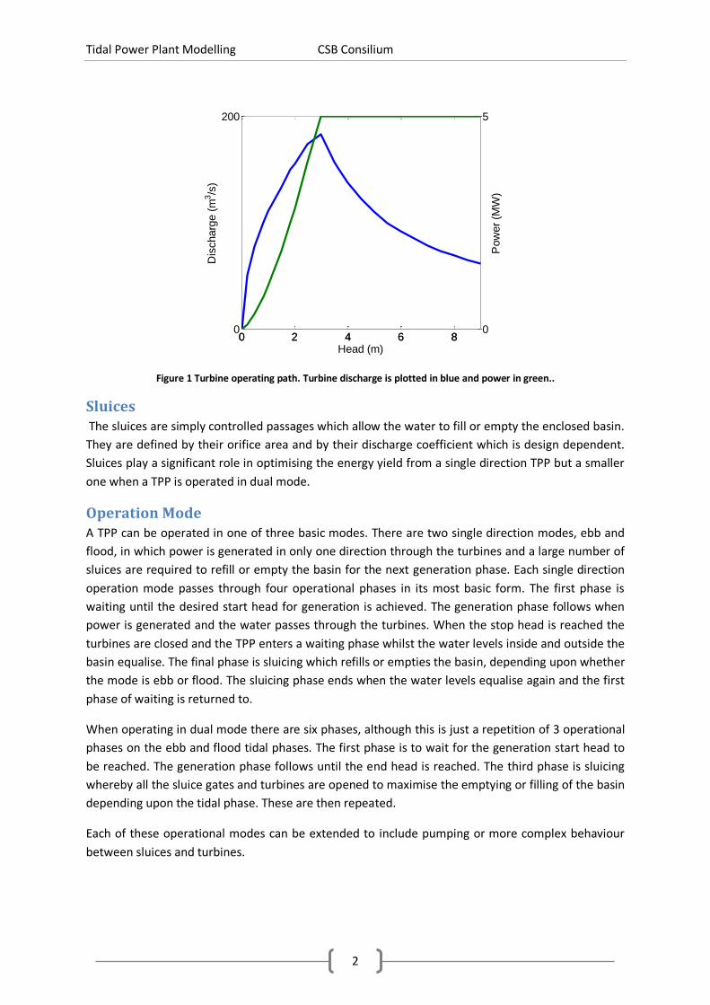
Turbines The turbines are modelled as operating paths which determine how the turbine operates for a

given head. Figure 1 shows an example turbine operating path which is used in the examples shown

below. The blue line shows the turbine discharge for a given head and the green line plots the power

output.

The turbine would usually have a different operating path for each direction and also when, and if, it

is used as a pump. When not generating power, the turbine can be operated in orifice mode. This

allows water to freely pass through in a similar way to a submerged sluice gate.


2

Figure 1 Turbine operating path. Turbine discharge is plotted in blue and power in green..

Sluices The sluices are simply controlled passages which allow the water to fill or empty the enclosed basin.

They are defined by their orifice area and by their discharge coefficient which is design dependent.

Sluices play a significant role in optimising the energy yield from a single direction TPP but a smaller

one when a TPP is operated in dual mode.

Operation Mode A TPP can be operated in one of three basic modes. There are two single direction modes, ebb and

flood, in which power is generated in only one direction through the turbines and a large number of

sluices are required to refill or empty the basin for the next generation phase. Each single direction

operation mode passes through four operational phases in its most basic form. The first phase is

waiting until the desired start head for generation is achieved. The generation phase follows when

power is generated and the water passes through the turbines. When the stop head is reached the

turbines are closed and the TPP enters a waiting phase whilst the water levels inside and outside the

basin equalise. The final phase is sluicing which refills or empties the basin, depending upon whether

the mode is ebb or flood. The sluicing phase ends when the water levels equalise again and the first

phase of waiting is returned to.

When operating in dual mode there are six phases, although this is just a repetition of 3 operational

phases on the ebb and flood tidal phases. The first phase is to wait for the generation start head to

be reached. The generation phase follows until the end head is reached. The third phase is sluicing

whereby all the sluice gates and turbines are opened to maximise the emptying or filling of the basin

depending upon the tidal phase. These are then repeated.

Each of these operational modes can be extended to include pumping or more complex behaviour

between sluices and turbines.

0 2 4 6 80

200

Head (m)

Dis

charg

e (

m3/s

)

0 2 4 6 80

5

Pow

er

(MW

)


3

0-D Modelling The 0-D model is simply a statement of the conservation of mass. That is the only change in the

volume of water in the enclosed basin of a TPP comes from water coming in or going out through

the turbines or sluices. This is written as

(1)

where V is the enclosed basin volume of water, t is the time and Q(H) is the discharge through the

turbines or gates for a given head H. The volume can be thought of as a sum of thin horizontal slices

of small thickness and this means that equation (1) can be written as

(2)

where z is the enclosed water level and S(z) is the horizontal surface area of the basin at water level

z. The head across the turbines or sluices is determined as the difference in water levels inside and

outside the basin, ie

(3)

where Y(t) is the prescribed external tide.

Theoretical Analysis If the bathymetry is assumed to be a known function and the discharge during the generation phase

is a constant value then the water level in the basin can be written analytically as

(4)

where z1 and z2 are the start and end water levels within the basin at the start and end generation

times t1 and t2. If the power is given by

(5)

where ρ is the density of water and g is the acceleration due to gravity, then the energy yield from a

single tide can be analytically calculated.

CSB Consilium Model The CSB Consilium model solves equation (2) using the discharges specified for the sluice gates and

turbines depending upon the phase of the operation currently underway. The turbine discharge is

defined through the use of the operating path, an example of which is shown in Figure 1. The

discharge of water through the turbines in orifice mode and through any submerged sluice gates is

given by

(6)


4

where ε is the discharge coefficient and A is the gate or orifice area. The model also includes the

standard equations for weir flow if the sluice gates are not fully submerged, however the turbines

are always assumed to be submerged.

The CSB Consilium model solves each operational mode so that the exact generation window can be

calculated. To achieve this, a variable time step 4th order accurate ODE solver is used. The turbine

operating path is an input to the program and any values needed are obtained through linear

interpolation. The bathymetry of the basin, S(z), is also an input parameter and again linear

interpolation is used to obtain exact values. The external tide can be specified as a time series or as a

set of tidal constituents. If the tide is a time series intermediate data is obtained through linear

interpolation, but if a set of tidal constituents is used exact values are calculated.

The outputs of the model are the full time series of water levels inside and outside of the basin, the

operating mode, number of turbines in use and power. The intertidal area is also calculated for each

simulation. The annual energy yield can be calculated in a number of ways. The simplest method is

using the trapezium method to integrate the power curve. The most complex method recalculates

the water levels inside and outside the basin within each generation window using a specified

number of points. These new water levels are then used to calculate the power output and this new

curve is integrated through the use of the trapezium rule. There can be significant differences (up to

10%) in the energy yield due to the method used.

Validation

To provide a validation of the modelling techniques used the 0-D model is compared with the

theoretical solution. A turbine is made which has a constant flux of 2000m3/s throughout the head

range and the basin is assumed to be a constant size of 10km2. The tide is set as a single M2

constituent with 3m amplitude. By fixing the generation start and end heads as 2m and 1m

0 5 10 15-3

-2

-1

0

1

2

3

Time (hrs)

Wate

r Level (m

MS

L)

Figure 2 Plot of the water levels inside and outside the TPP basin. Theoretical solution shown in blue (external) and green (basin). CSB Consilium model shown in

black dashed (external) and red dashed (basin).


5

respectively the water levels, power output and energy yield for a single tide can be calculated and

compared.

Figure 2 shows the water levels for the theoretical and CSB Consilium models. It is clearly shown that

the water levels are identical between the two models which shows that the numerical methods

used in the CSB Consilium model are accurate.

The annual energy yield predicted by the theoretical model is 205.1GWh/y. The simple trapezium

rule based upon the time series output from the 0-D model predicts 211.4GWh/y and the more

complex integration method gives 205.1GWh/y. For energy yield reporting from the 0-D model the

complex methodology is used exclusively.


6

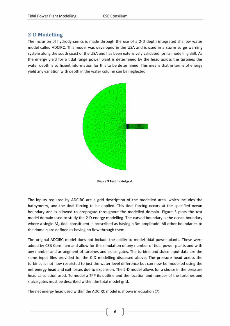
2-D Modelling The inclusion of hydrodynamics is made through the use of a 2-D depth integrated shallow water

model called ADCIRC. This model was developed in the USA and is used in a storm surge warning

system along the south coast of the USA and has been extensively validated for its modelling skill. As

the energy yield for a tidal range power plant is determined by the head across the turbines the

water depth is sufficient information for this to be determined. This means that in terms of energy

yield any variation with depth in the water column can be neglected.

Figure 3 Test model grid.

The inputs required by ADCIRC are a grid description of the modelled area, which includes the

bathymetry, and the tidal forcing to be applied. This tidal forcing occurs at the specified ocean

boundary and is allowed to propogate throughout the modelled domain. Figure 3 plots the test

model domain used to study the 2-D energy modelling. The curved boundary is the ocean boundary

where a single M2 tidal constituent is prescribed as having a 3m amplitude. All other boundaries to

the domain are defined as having no flow through them.

The original ADCIRC model does not include the ability to model tidal power plants. These were

added by CSB Consilium and allow for the simulation of any number of tidal power plants and with

any number and arrangment of turbines and sluice gates. The turbine and sluice input data are the

same input files provided for the 0-D modelling discussed above. The pressure head across the

turbines is not now restricted to just the water level difference but can now be modelled using the

net energy head and exit losses due to expansion. The 2-D model allows for a choice in the pressure

head calculation used. To model a TPP its outline and the location and number of the turbines and

sluice gates must be described within the total model grid.

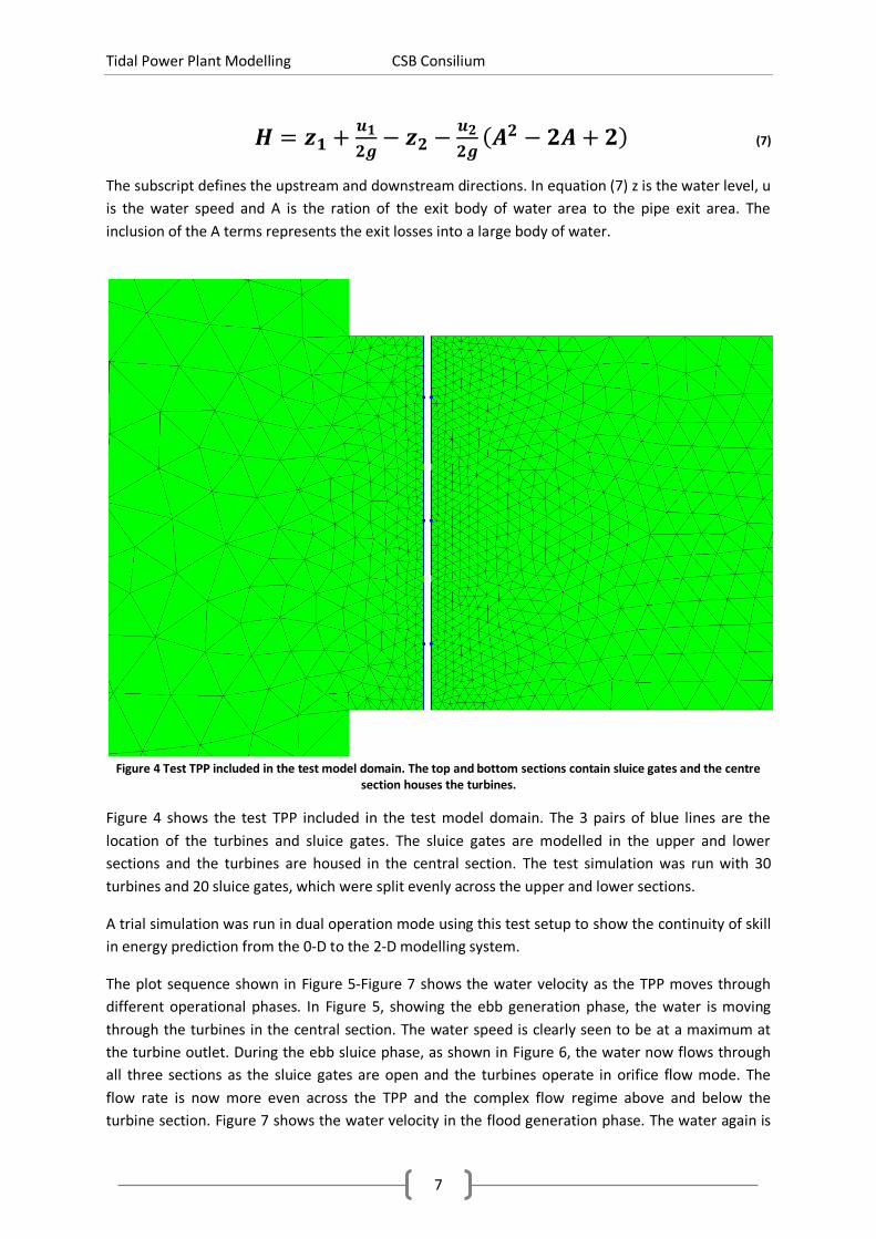
The net energy head used within the ADCIRC model is shown in equation (7).


7

(7)

The subscript defines the upstream and downstream directions. In equation (7) z is the water level, u

is the water speed and A is the ration of the exit body of water area to the pipe exit area. The

inclusion of the A terms represents the exit losses into a large body of water.

Figure 4 Test TPP included in the test model domain. The top and bottom sections contain sluice gates and the centre

section houses the turbines.

Figure 4 shows the test TPP included in the test model domain. The 3 pairs of blue lines are the

location of the turbines and sluice gates. The sluice gates are modelled in the upper and lower

sections and the turbines are housed in the central section. The test simulation was run with 30

turbines and 20 sluice gates, which were split evenly across the upper and lower sections.

A trial simulation was run in dual operation mode using this test setup to show the continuity of skill

in energy prediction from the 0-D to the 2-D modelling system.

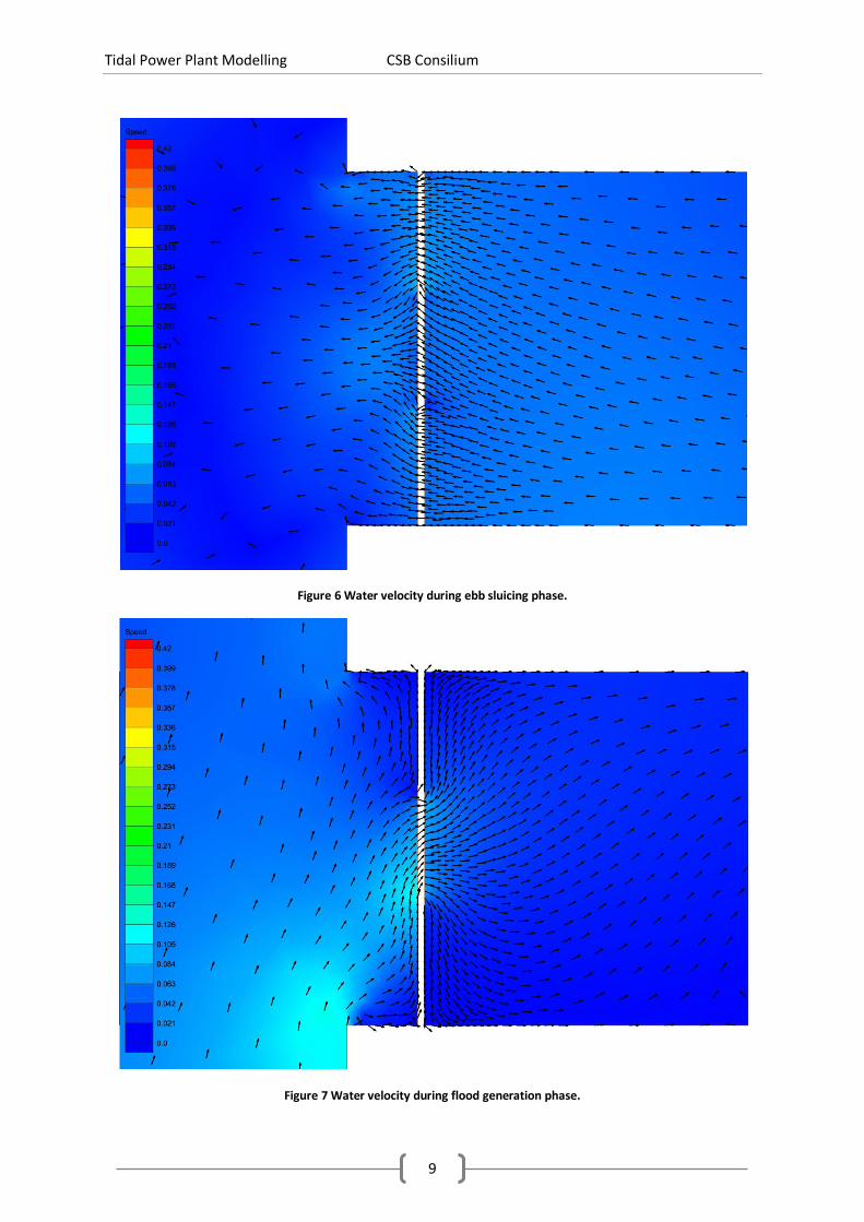
The plot sequence shown in Figure 5-Figure 7 shows the water velocity as the TPP moves through

different operational phases. In Figure 5, showing the ebb generation phase, the water is moving

through the turbines in the central section. The water speed is clearly seen to be at a maximum at

the turbine outlet. During the ebb sluice phase, as shown in Figure 6, the water now flows through

all three sections as the sluice gates are open and the turbines operate in orifice flow mode. The

flow rate is now more even across the TPP and the complex flow regime above and below the

turbine section. Figure 7 shows the water velocity in the flood generation phase. The water again is


8

only flowing through the turbines although now the flow speeds are less than in the ebb generation

phase. This is due to the differential turbine operation in the ebb and flood directions.

Figure 5 Water velocity during ebb generation phase.


9

Figure 6 Water velocity during ebb sluicing phase.

Figure 7 Water velocity during flood generation phase.


10

The water levels at two points, one on each side of the turbines, were extracted as time series. The

0-D model was run using 30 turbines and 20 sluice gates with a tidal amplitude of 3.046m which was

extracted from the 2-D model at the location of the water level data on the external side. Figure 8

shows the water level data from the 2-D and 0-D models overlaid. The external tide data shown in

green (2-D) and black (0-D) are virtually identical and no difference between them can be seen in the

plot. The simple nature of the tide in containing only one tidal constituent makes this matching

possible and it is unlikely to be as exact when a realistic tidal forcing is used in a real world

simulation. The water levels within the enclosed basin are shown in blue (2-D) and red (0-D). The

inclusion of the hydrodynamics in the 2-D model is shown in the wavy nature of the blue line when

compared to the smooth red line of the 0-D model. The 2-D model water levels follow the trend of

the 0-D model which is as much as could be expected from this comparison.

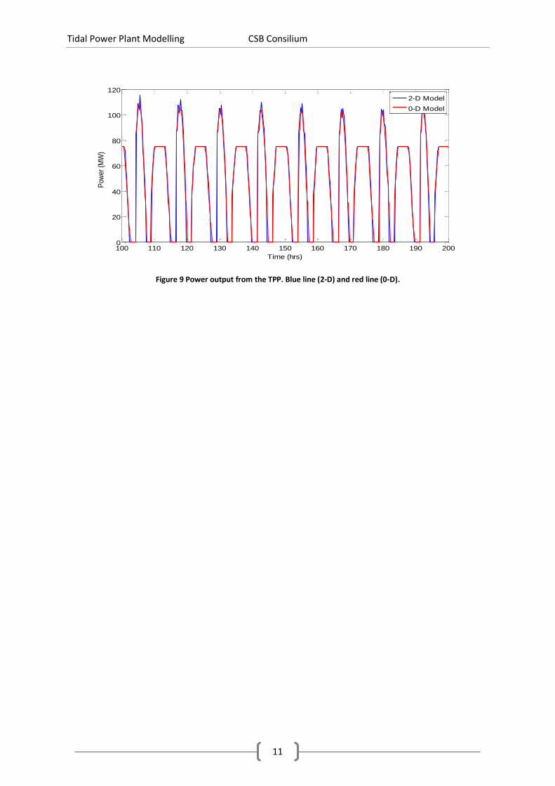
The power output from the TPP is shown in Figure 9 for both the 2-D (blue line) and 0-D (red line)

models. The power output from the 0-D model is smooth whereas the highly variable nature of the

water level within the enclosed basin about the 0-D result is reflected in the power output from the

2-D model. Overall the two models have an excellent agreement in prediction.

The annual energy yield in the 2-D model can only be calculated from the simple trapezium method.

To allow for a reasonable comparison of energy predictions between the 0-D and 2-D models the

energy yield is calculated in the 0-D model using both the trapezium method and the complex

method. The 2-D energy yield is compared with the 0-D trapezium method and then scaled to the

complex result.

Figure 8 Water levels inside and outside the basin. The external water levels are shown in green (2-D) and black (0-D). The basin water level is shown in blue (2-D) and red (0-D).

100 110 120 130 140 150 160 170 180 190 200-4

-3

-2

-1

0

1

2

3

4

Time (hrs)

Wat

er L

evel

(m

MS

L)


11

Figure 9 Power output from the TPP. Blue line (2-D) and red line (0-D).

100 110 120 130 140 150 160 170 180 190 2000

20

40

60

80

100

120

Time (hrs)

Pow

er (

MW

)

2-D Model

0-D Model


12

Contact Details Author Dr Ian Walkington CSB Consilium 9 Izaak Walton Way Madeley CW3 9NA Tel: +44 (0)1782 497767 e-mail: [email protected]

Tidal Power Plant Modelling - CSB Consilium -...

Documents

Transcript of Tidal Power Plant Modelling - CSB Consilium -...