Aerodynamics

Lecture 6:

Boundary Layer Solutions

G. Dimitriadis

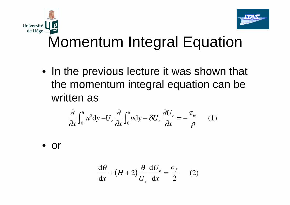
Momentum Integral Equation

• In the previous lecture it was shown that

the momentum integral equation can be

written as

• or

xu2dy

0Ue x

udy0

Ue

Ue

x=

w (1)

d

dx+ H + 2( )

Ue

dUe

dx=c f2

(2)

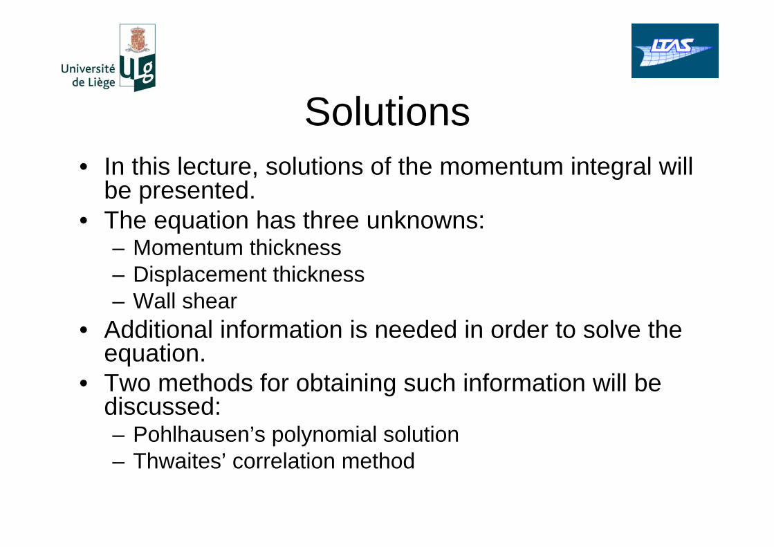
Solutions

• In this lecture, solutions of the momentum integral will be presented.

• The equation has three unknowns: – Momentum thickness

– Displacement thickness

– Wall shear

• Additional information is needed in order to solve the equation.

• Two methods for obtaining such information will be discussed: – Pohlhausen’s polynomial solution

– Thwaites’ correlation method

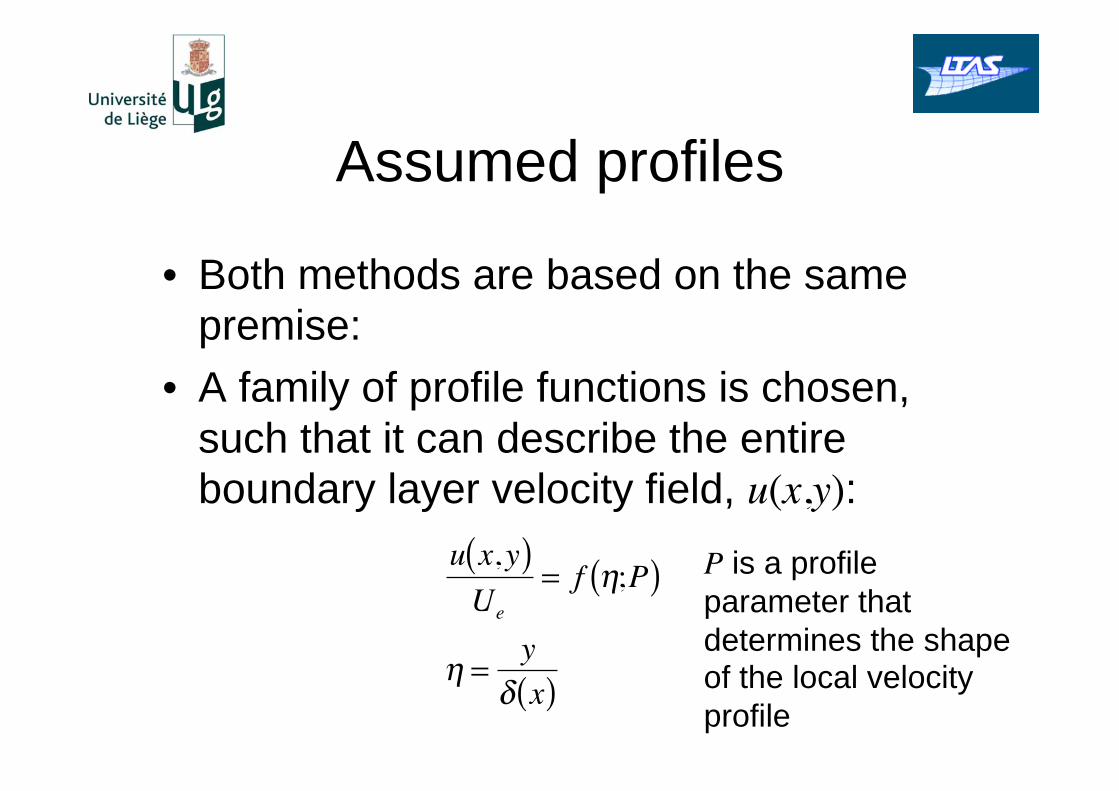
Assumed profiles

• Both methods are based on the same

premise:

• A family of profile functions is chosen,

such that it can describe the entire

boundary layer velocity field, u(x,y):

u x,y( )Ue

= f ;P( )

=y

x( )

P is a profile

parameter that

determines the shape of the local velocity

profile

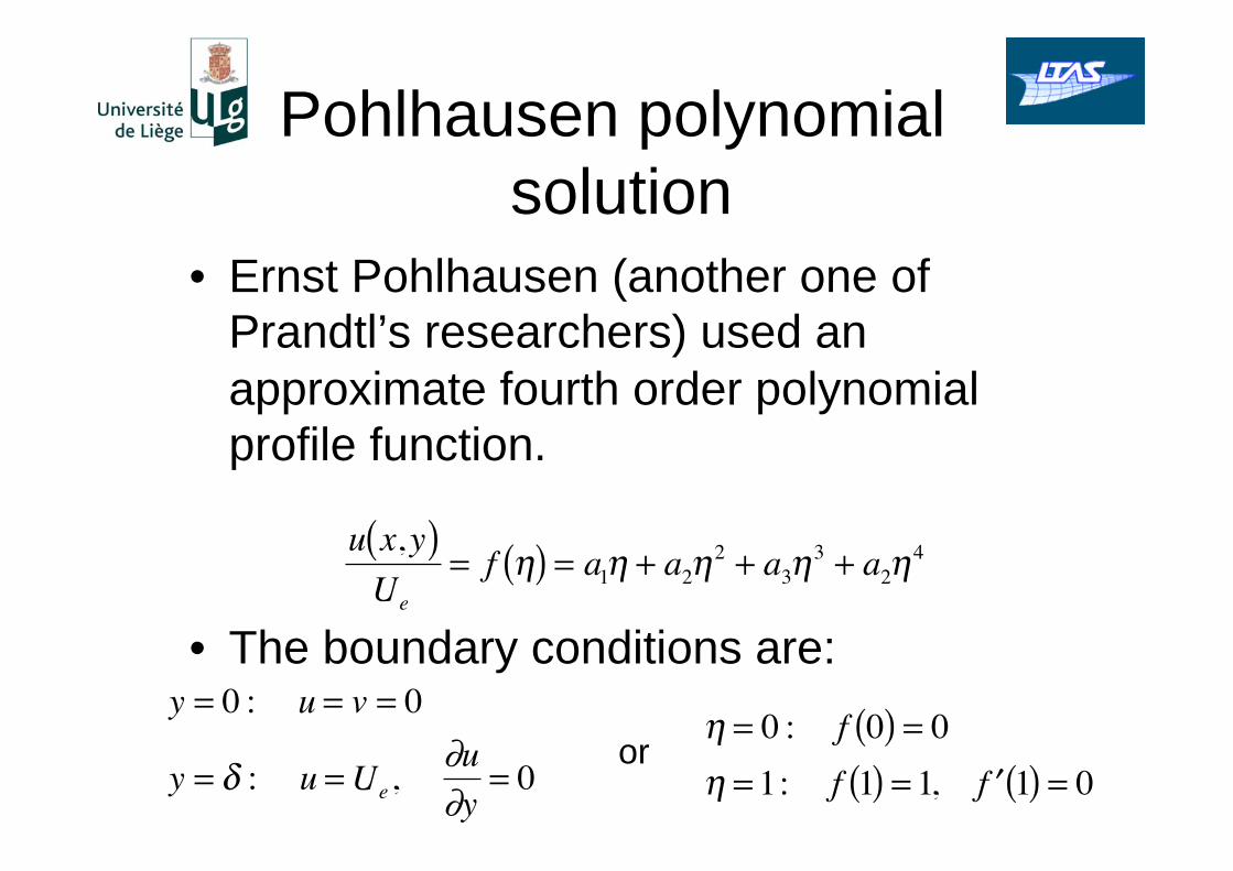
Pohlhausen polynomial

solution

• Ernst Pohlhausen (another one of

Prandtl’s researchers) used an

approximate fourth order polynomial

profile function.

• The boundary conditions are:

u x,y( )Ue

= f ( ) = a1 + a22+ a3

3+ a2

4

y = 0 : u = v = 0

y = : u =Ue, u

y= 0

= 0 : f 0( ) = 0

= 1: f 1( ) = 1, f 1( ) = 0or

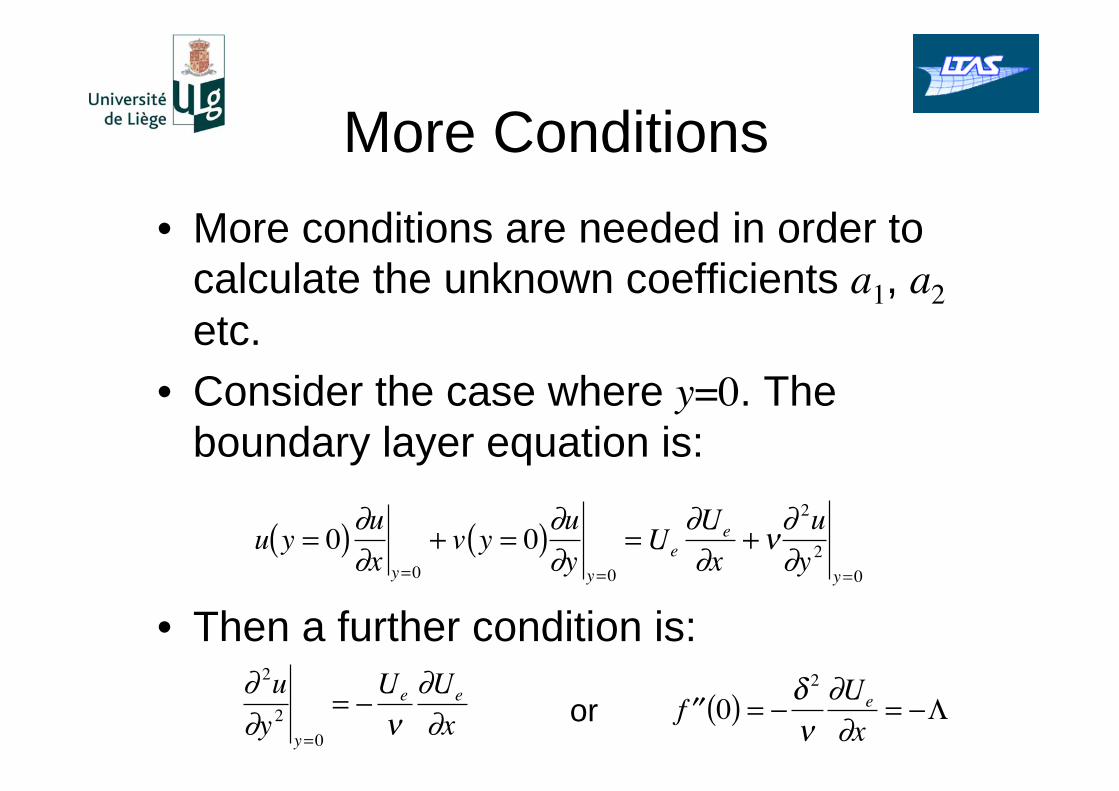
More Conditions

• More conditions are needed in order to

calculate the unknown coefficients a1, a2 etc.

• Consider the case where y=0. The

boundary layer equation is:

• Then a further condition is:

u y = 0( )u

x y=0

+ v y = 0( )u

yy=0

=Ue

Ue

x+

2u

y 2y=0

2u

y 2y=0

=Ue Ue

x f 0( ) =

2 Ue

x=or

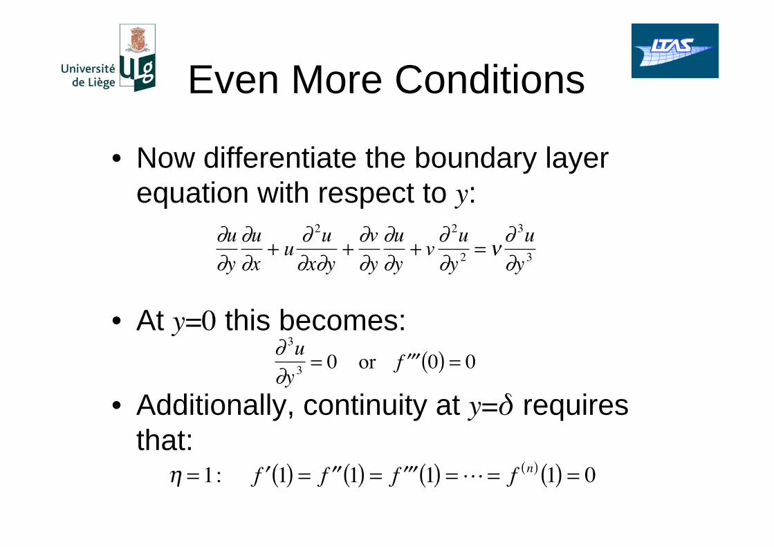
Even More Conditions

• Now differentiate the boundary layer

equation with respect to y:

• At y=0 this becomes:

• Additionally, continuity at y= requires

that:

u

y

u

x+ u

2u

x y+

v

y

u

y+ v

2u

y 2=

3u

y 3

3u

y 3 = 0 or f 0( ) = 0

= 1: f 1( ) = f 1( ) = f 1( ) = = f n( ) 1( ) = 0

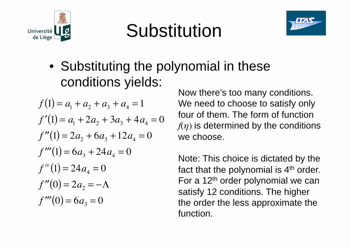
Substitution

• Substituting the polynomial in these

conditions yields:

f 1( ) = a1 + a2 + a3 + a4 = 1

f 1( ) = a1 + 2a2 + 3a3 + 4a4 = 0

f 1( ) = 2a2 + 6a3 +12a4 = 0

f 1( ) = 6a3 + 24a4 = 0

f iv 1( ) = 24a4 = 0

f 0( ) = 2a2 =

f 0( ) = 6a3 = 0

Now there’s too many conditions.

We need to choose to satisfy only

four of them. The form of function f( ) is determined by the conditions

we choose.

Note: This choice is dictated by the

fact that the polynomial is 4th order.

For a 12th order polynomial we can

satisfy 12 conditions. The higher

the order the less approximate the

function.

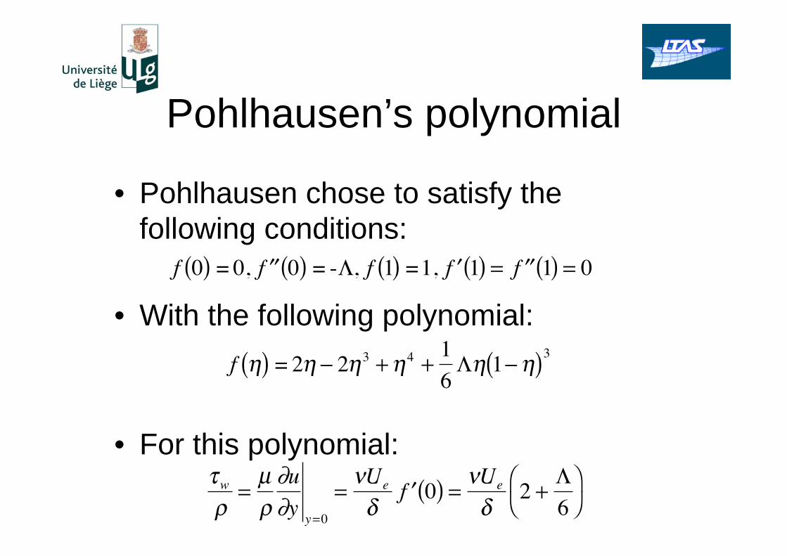
Pohlhausen’s polynomial

• Pohlhausen chose to satisfy the

following conditions:

• With the following polynomial:

• For this polynomial:

f 0( ) = 0, f 0( ) = - , f 1( ) =1, f 1( ) = f 1( ) = 0

f ( ) = 2 2 3+

4+1

61( )

3

w =μ u

yy =0

=Ue f 0( ) =

Ue 2 +6

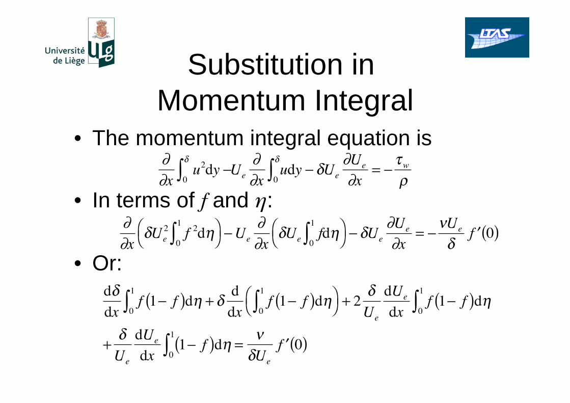
Substitution in

Momentum Integral • The momentum integral equation is

• In terms of f and :

• Or:

xu2dy

0Ue x

udy0

Ue

Ue

x=

w

xUe2 f 2d0

1

Ue xUe fd

0

1

Ue

Ue

x=

Ue f 0( )

d

dxf 1 f( )d

0

1+

d

dxf 1 f( )d

0

1

+ 2Ue

dUe

dxf 1 f( )d

0

1

+Ue

dUe

dx1 f( )d

0

1=

Ue

f 0( )

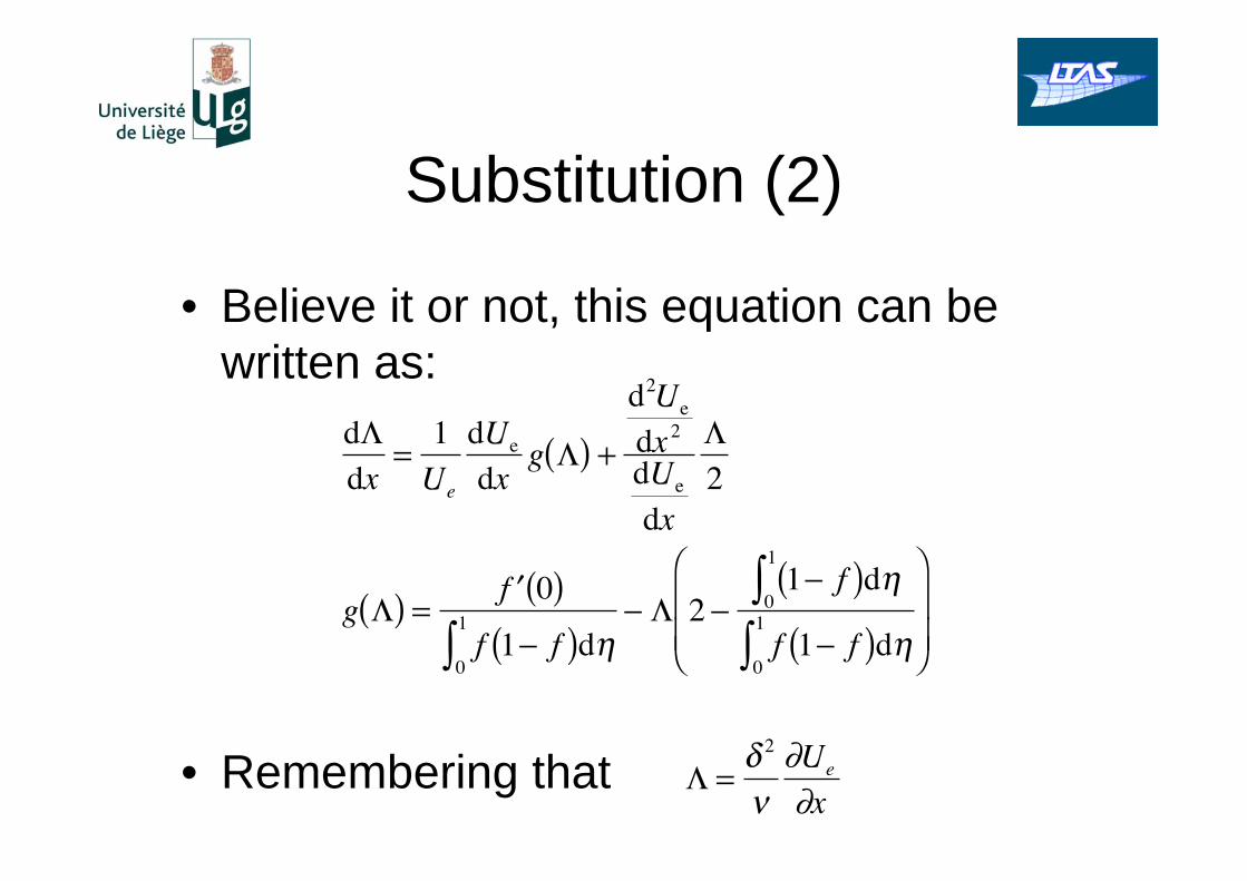
Substitution (2)

• Believe it or not, this equation can be

written as:

• Remembering that

ddx

=1

Ue

dUe

dxg( ) +

d2Ue

dx 2

dUe

dx2

g( ) = f 0( )

f 1 f( )d0

1 21 f( )d

0

1

f 1 f( )d0

1

=

2 Ue

x

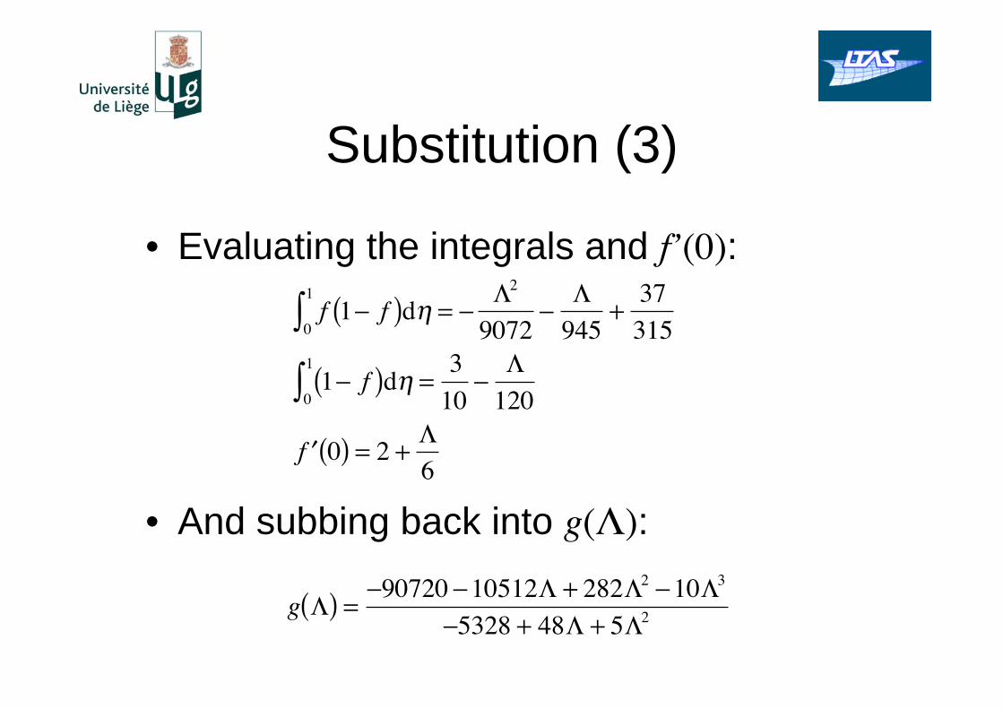
Substitution (3)

• Evaluating the integrals and f’(0):

• And subbing back into g( ):

f 1 f( )d0

1=

2

9072 945+37315

1 f( )d0

1=3

10 120

f 0( ) = 2 +6

g( ) =90720 10512 + 282 2 10 3

5328 + 48 + 5 2

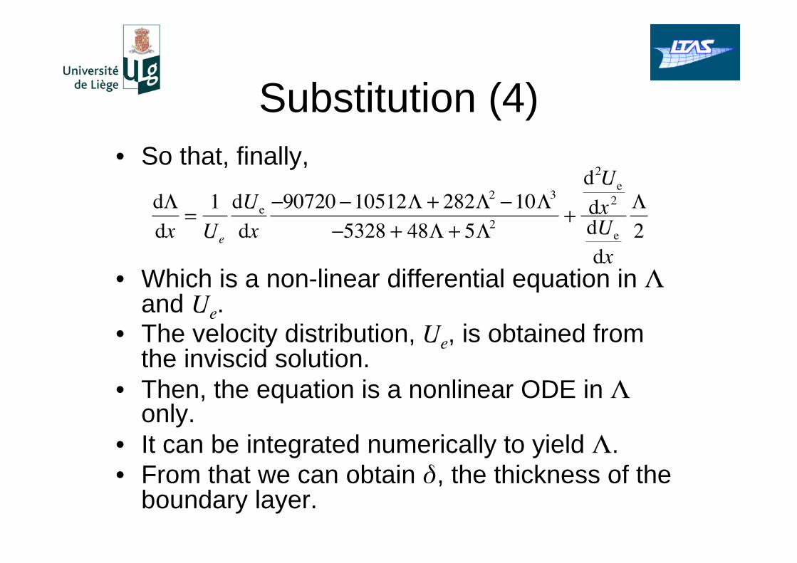
Substitution (4)

• So that, finally,

• Which is a non-linear differential equation in and Ue.

• The velocity distribution, Ue, is obtained from the inviscid solution.

• Then, the equation is a nonlinear ODE in only.

• It can be integrated numerically to yield .

• From that we can obtain , the thickness of the boundary layer.

d

dx=1

Ue

dUe

dx

90720 10512 + 282 2 10 3

5328 + 48 + 5 2 +

d2Ue

dx 2

dUe

dx2

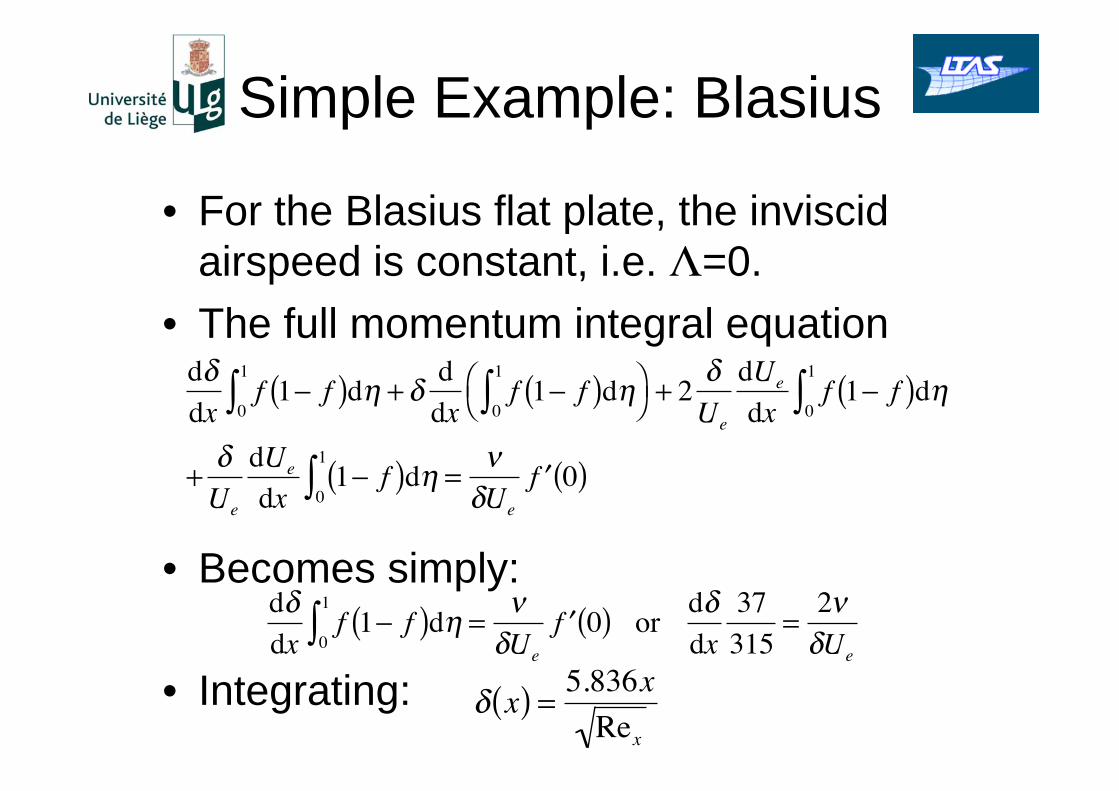
Simple Example: Blasius

• For the Blasius flat plate, the inviscid

airspeed is constant, i.e. =0.

• The full momentum integral equation

• Becomes simply:

• Integrating:

d

dxf 1 f( )d

0

1+

d

dxf 1 f( )d

0

1

+ 2Ue

dUe

dxf 1 f( )d

0

1

+Ue

dUe

dx1 f( )d

0

1=

Ue

f 0( )

d

dxf 1 f( )d

0

1=

Ue

f 0( ) or d

dx

37

315=

2

Ue

x( ) =5.836x

Rex

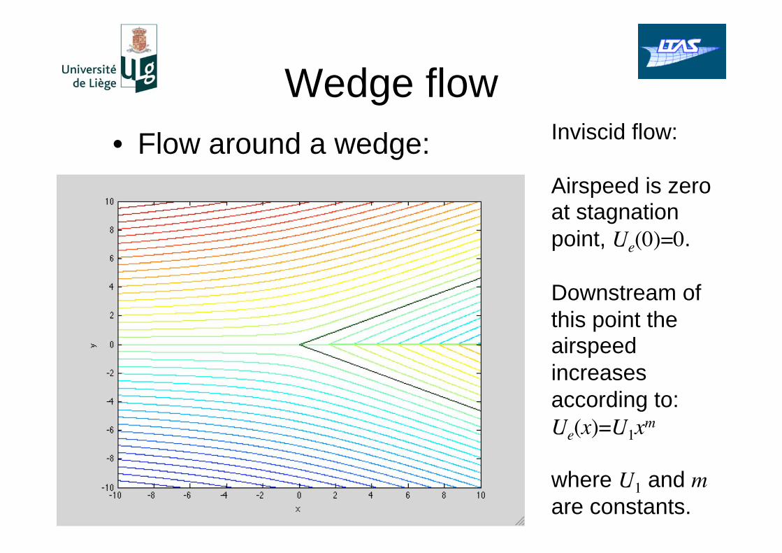
Wedge flow

• Flow around a wedge: Inviscid flow:

Airspeed is zero at stagnation

point, Ue(0)=0.

Downstream of

this point the airspeed

increases

according to:

Ue(x)=U1xm

where U1 and m

are constants.

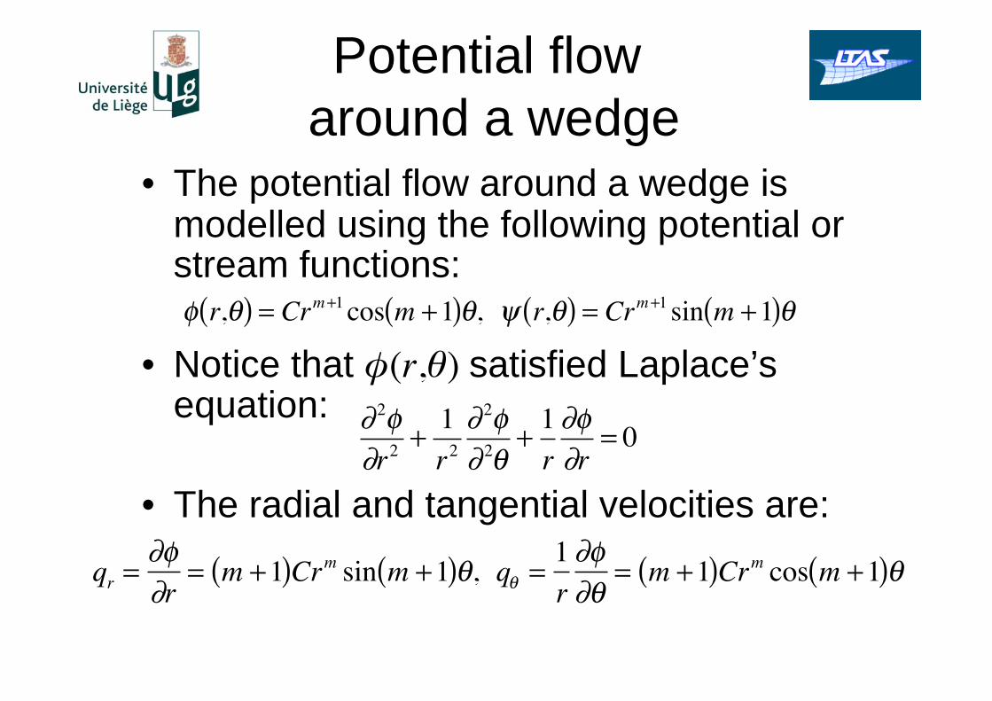
Potential flow

around a wedge • The potential flow around a wedge is

modelled using the following potential or stream functions:

• Notice that (r, ) satisfied Laplace’s equation:

• The radial and tangential velocities are:

r,( ) = Crm+1 cos m +1( ) , r,( ) = Crm+1 sin m +1( )

2

r2+1

r2

2

2 +1

r r= 0

qr = r= m +1( )Crm sin m +1( ) , q =

1

r= m +1( )Crm cos m +1( )

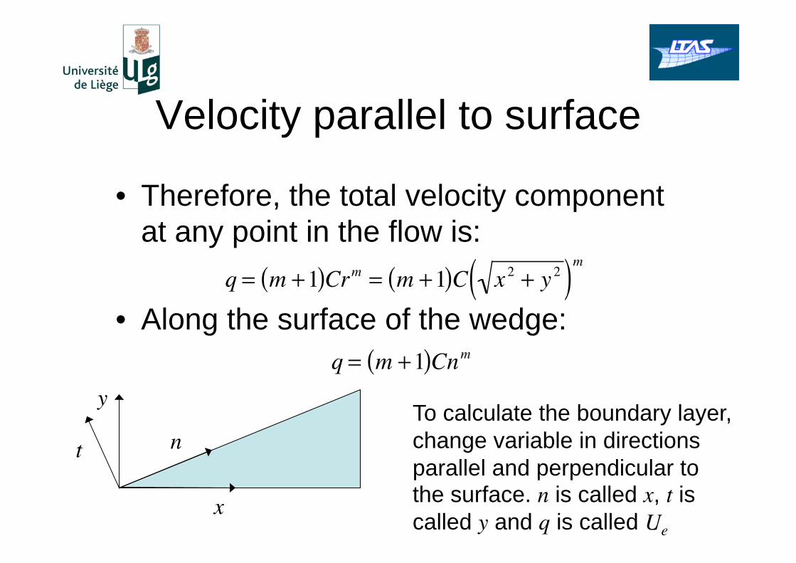
Velocity parallel to surface

• Therefore, the total velocity component

at any point in the flow is:

• Along the surface of the wedge:

q = m +1( )Crm = m +1( )C x 2 + y 2( )m

q = m +1( )Cnm

x

y

nTo calculate the boundary layer,

change variable in directions

parallel and perpendicular to the surface. n is called x, t is

called y and q is called Ue

t

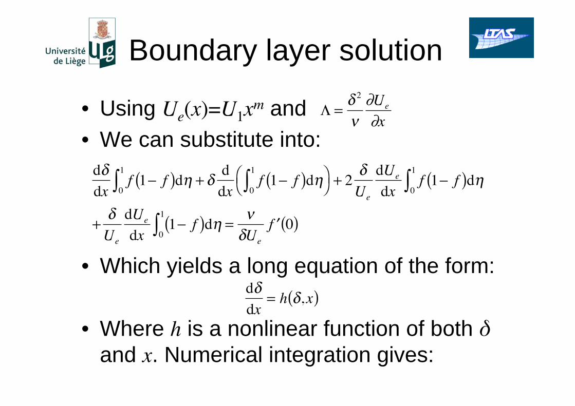
Boundary layer solution

• Using Ue(x)=U1xm and

• We can substitute into:

• Which yields a long equation of the form:

• Where h is a nonlinear function of both

and x. Numerical integration gives:

=

2 Ue

x

d

dxf 1 f( )d

0

1+

d

dxf 1 f( )d

0

1

+ 2Ue

dUe

dxf 1 f( )d

0

1

+Ue

dUe

dx1 f( )d

0

1=

Ue

f 0( )

d

dx= h ,x( )

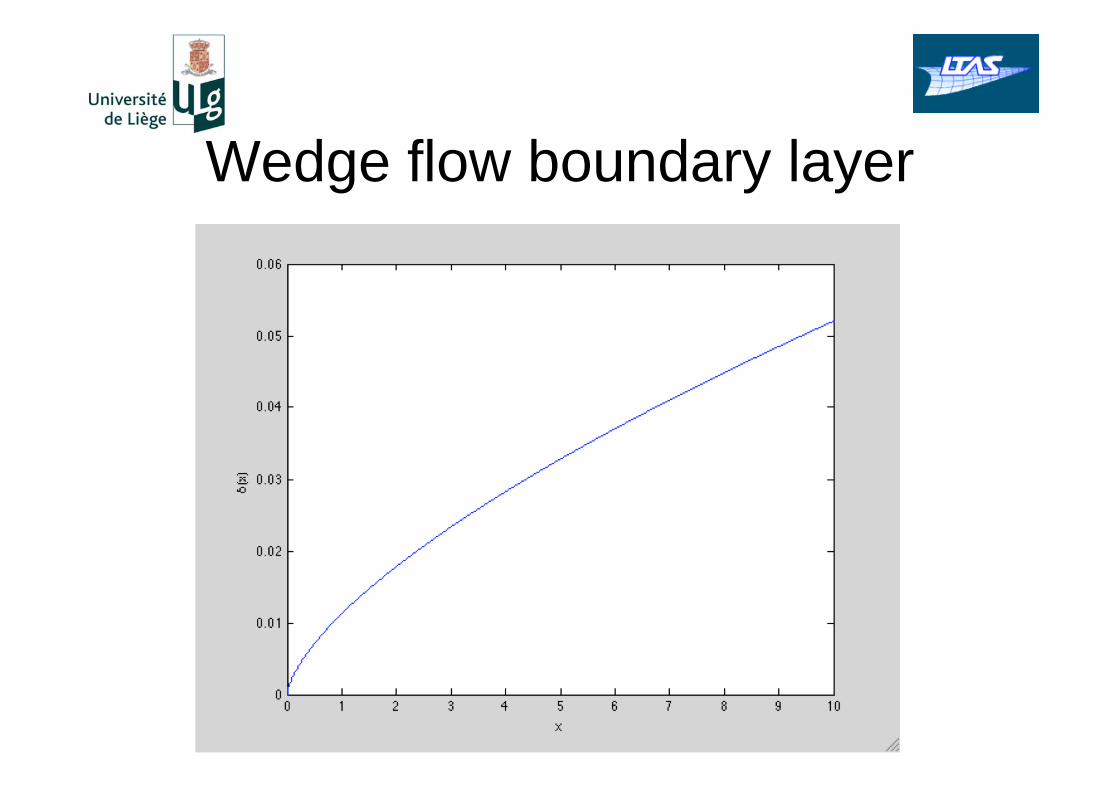
Wedge flow boundary layer

More about wedge flows

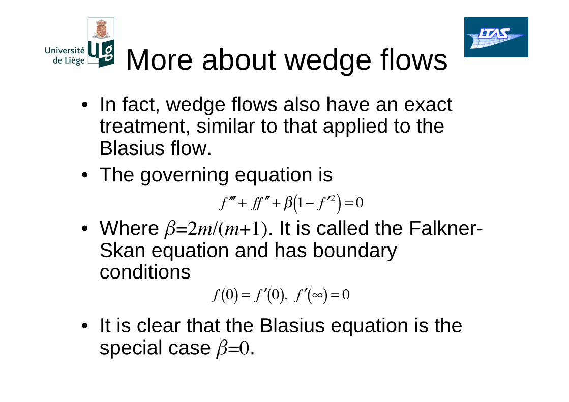
• In fact, wedge flows also have an exact treatment, similar to that applied to the Blasius flow.

• The governing equation is

• Where =2m/(m+1). It is called the Falkner-Skan equation and has boundary conditions

• It is clear that the Blasius equation is the special case =0.

f + f f + 1 f 2( ) = 0

f 0( ) = f 0( ), f ( ) = 0

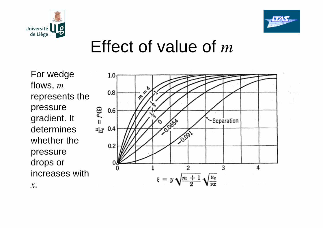
Effect of value of m

For wedge

flows, m

represents the pressure

gradient. It

determines

whether the

pressure drops or

increases with

x.

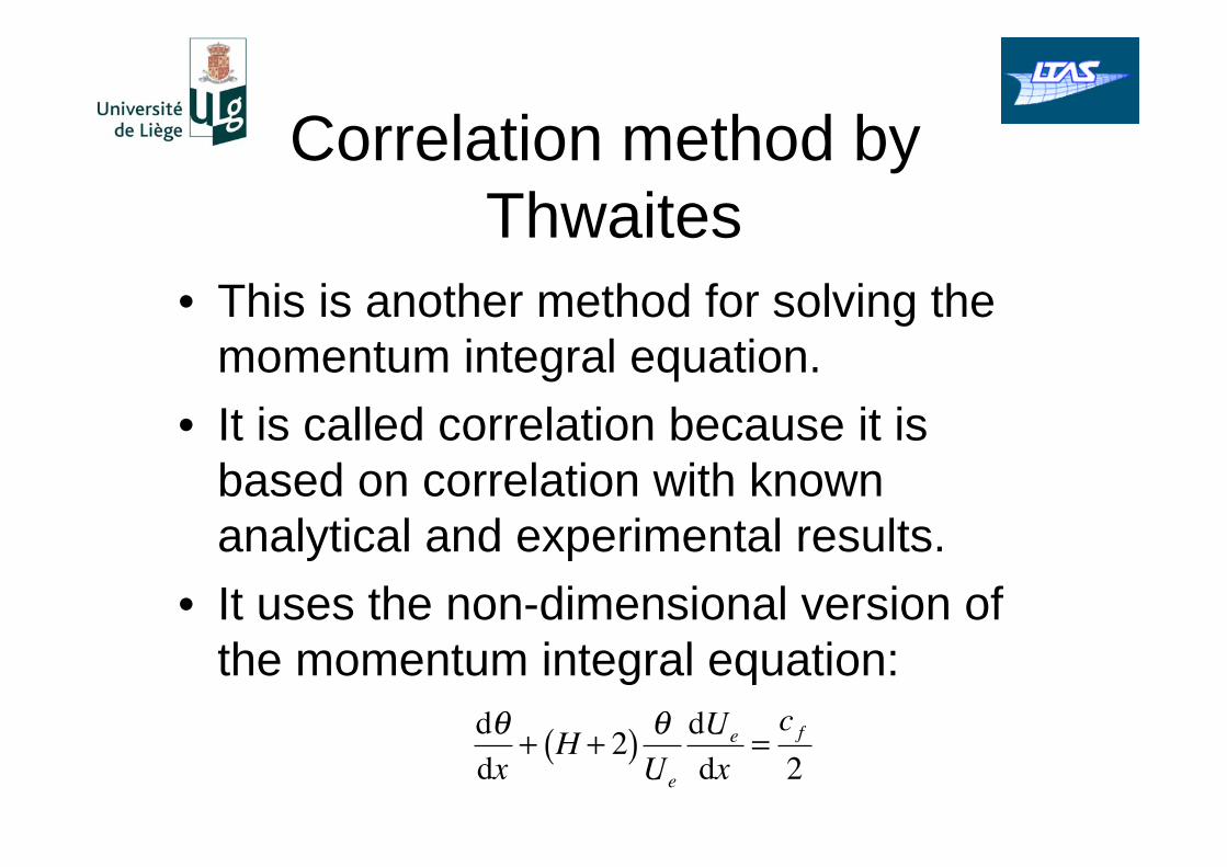
Correlation method by

Thwaites

• This is another method for solving the

momentum integral equation.

• It is called correlation because it is

based on correlation with known

analytical and experimental results.

• It uses the non-dimensional version of

the momentum integral equation:

d

dx+ H + 2( )

Ue

dUe

dx=c f2

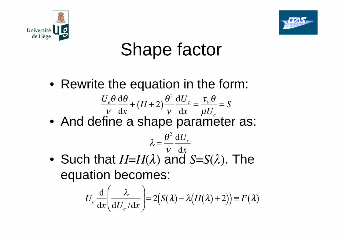
Shape factor

• Rewrite the equation in the form:

• And define a shape parameter as:

• Such that H=H( ) and S=S( ). The

equation becomes:

Ue d

dx+ H + 2( )

2 dUe

dx= w

μUe

= S

=

2 dUe

dx

Ue

d

dx dUe /dx

= 2 S( ) H( ) + 2( )( ) F( )

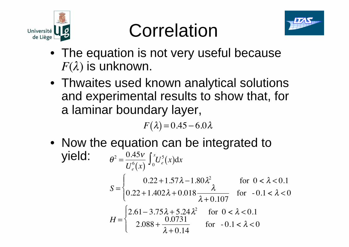
Correlation • The equation is not very useful because F( ) is unknown.

• Thwaites used known analytical solutions and experimental results to show that, for a laminar boundary layer,

• Now the equation can be integrated to yield:

F( ) = 0.45 6.0

2=

0.45

Ue6 x( )

Ue5 x( )dx

0

x

S =0.22 + 1.57 1.80 2 for 0 < < 0.1

0.22 + 1.402 + 0.018+ 0.107

for - 0.1 < < 0

H =2.61 3.75 + 5.24 2 for 0 < < 0.1

2.088 +0.0731

+ 0.14for - 0.1 < < 0

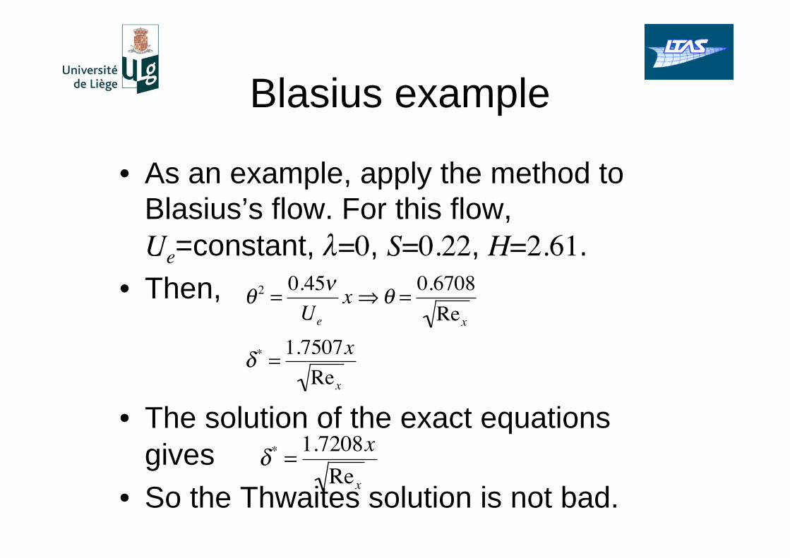
Blasius example

• As an example, apply the method to

Blasius’s flow. For this flow,

Ue=constant, =0, S=0.22, H=2.61.

• Then,

• The solution of the exact equations

gives

• So the Thwaites solution is not bad.

2=0.45

Ue

x =0.6708

Rex

*=1.7507x

Rex

*=1.7208x

Rex

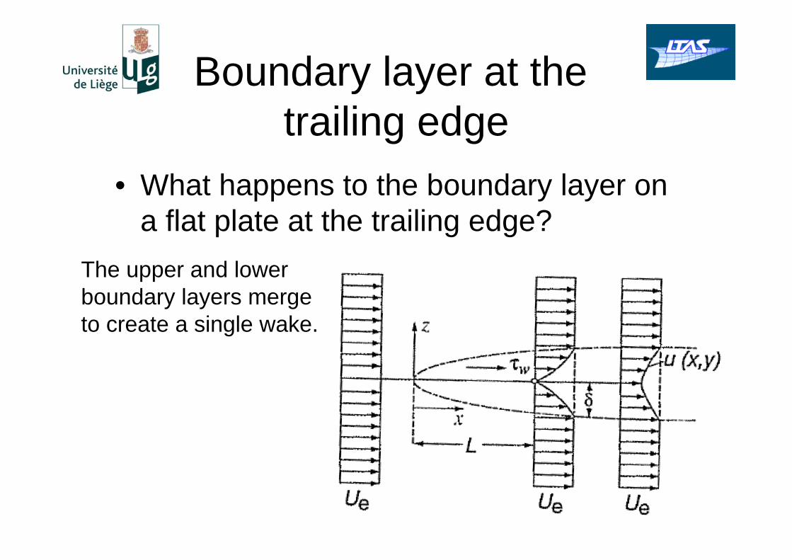
Boundary layer at the

trailing edge

• What happens to the boundary layer on

a flat plate at the trailing edge?

The upper and lower

boundary layers merge

to create a single wake.

Methods for airfoils

• In practice, the viscous flow over 2D airfoils is solved using an iterative method.

• The method is called viscous-inviscid interaction.

• The boundary layer solution requires an inviscid solution.

• However, once the boundary layer is calculated, it has a thickness that changes slightly the shape of the airfoil.

• Then, the inviscid solution must be recalculated for the airfoil + boundary layer.

• The new inviscid solution is used to calculate a new boundary layer.

• The new airfoil+boundary layer give rise to a new inviscid solution.

• Eventually the method converges.

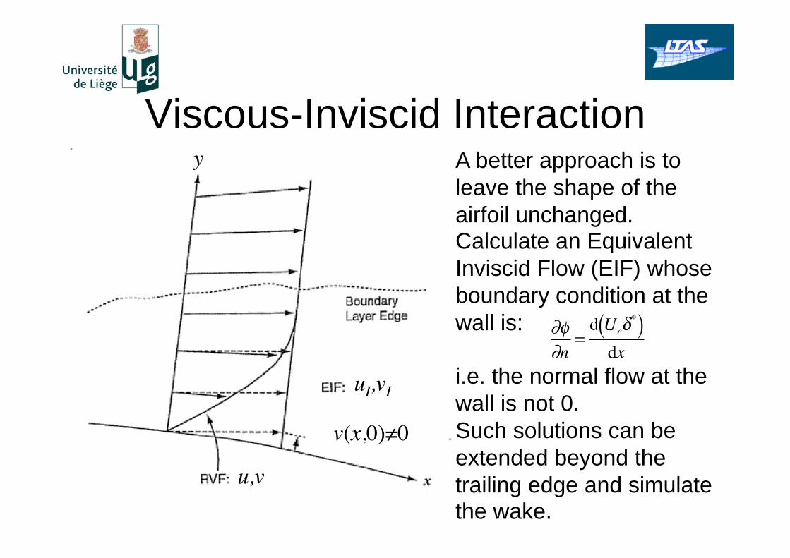
Viscous-Inviscid Interaction A better approach is to

leave the shape of the

airfoil unchanged. Calculate an Equivalent

Inviscid Flow (EIF) whose

boundary condition at the

wall is:

i.e. the normal flow at the

wall is not 0.

Such solutions can be

extended beyond the

trailing edge and simulate the wake.

n=d Ue

*( )dx

y

uI,vI

u,v

v(x,0) 0

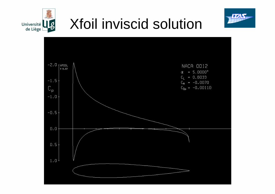
Xfoil inviscid solution

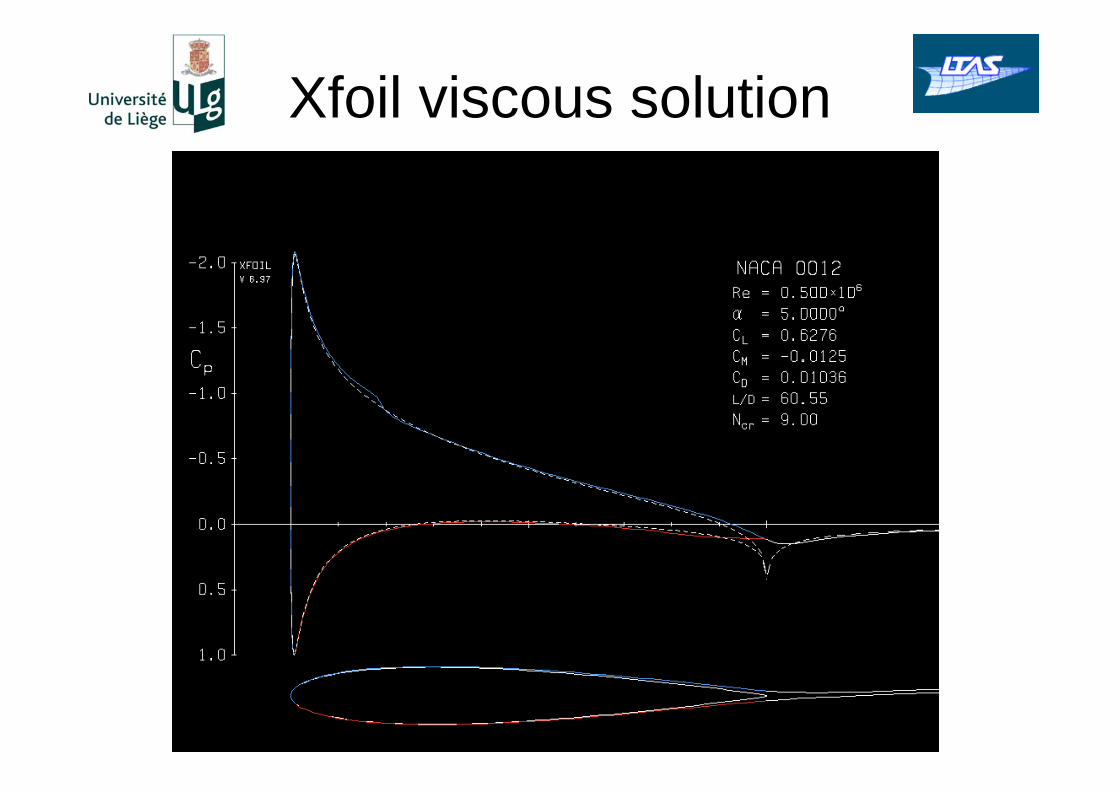
Xfoil viscous solution

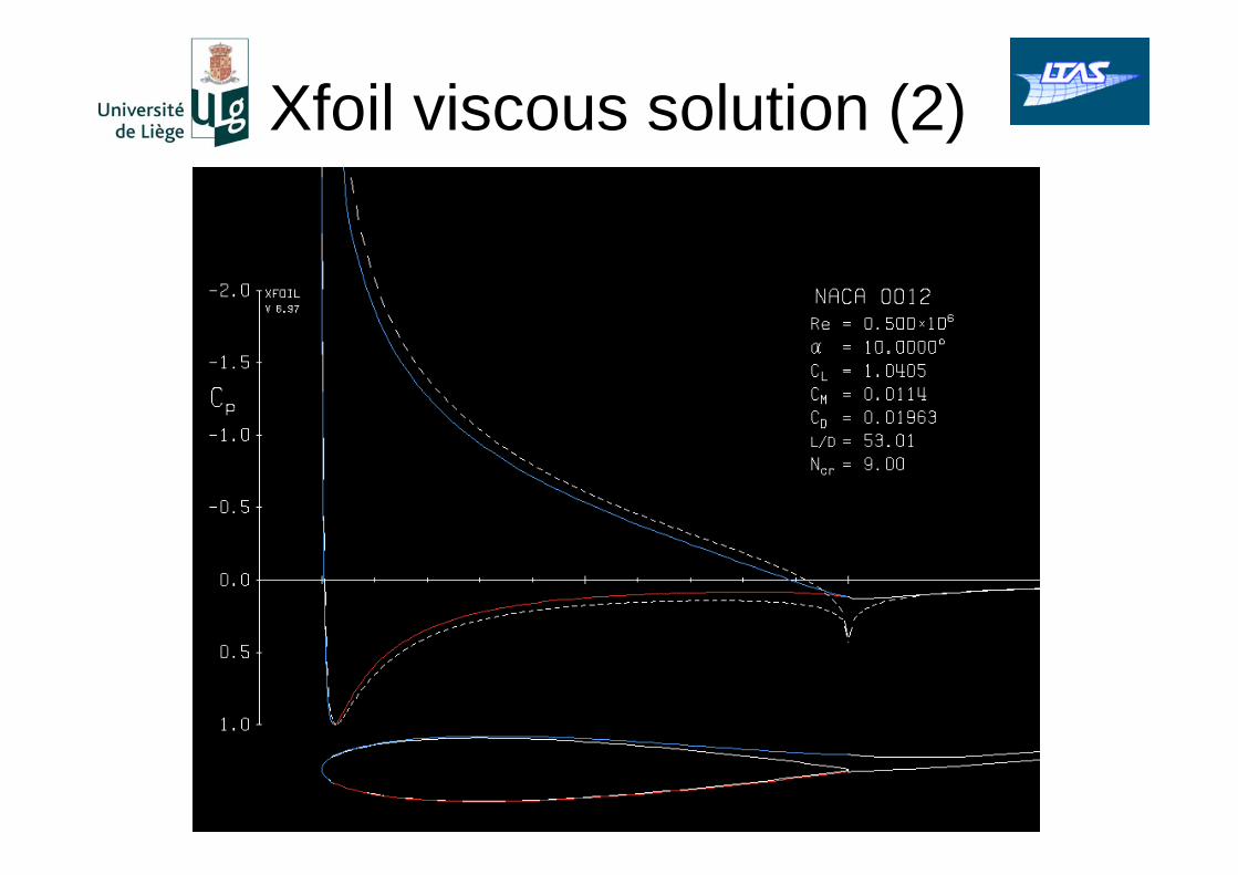
Xfoil viscous solution (2)

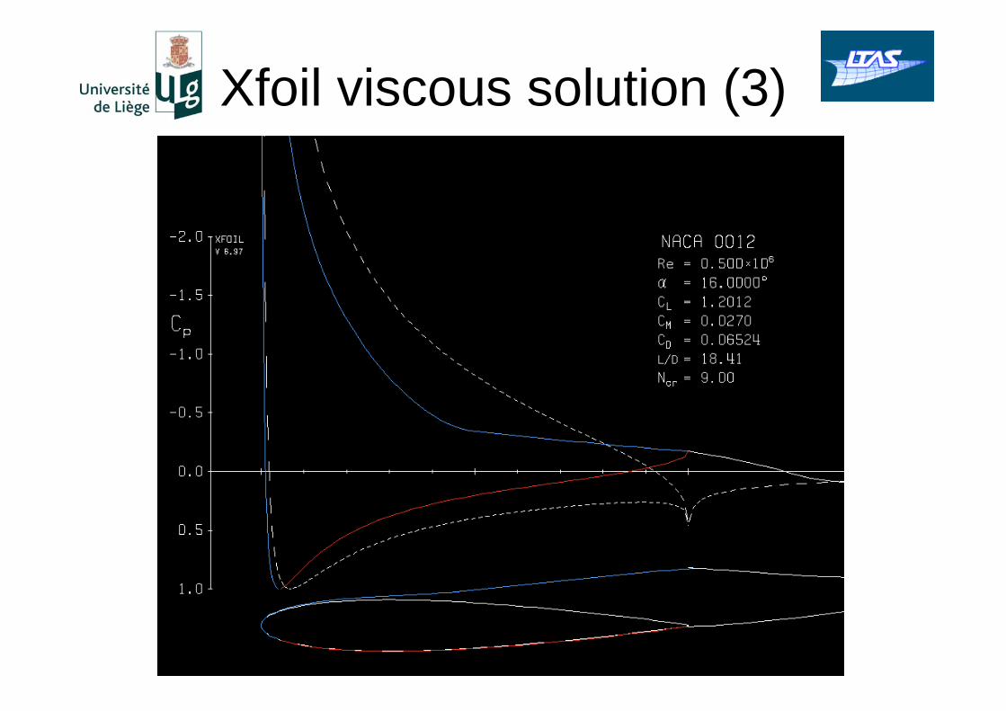
Xfoil viscous solution (3)

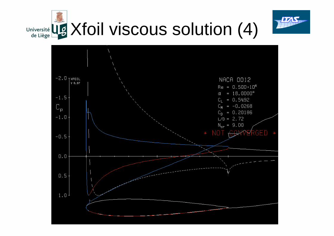
Xfoil viscous solution (4)