1

Thunderstorm Dynamics Helicity and Hodographs and their effect on thunderstorm longevity Bluestein Vol II. Pages 471-476. Dowsell, 1991: A REVIEW FOR FORECASTERS ON THE APPLICATION OF HODOGRAPHS TO FORECASTING SEVERE THUNDERSTORMS. National Weather Digest, 16 (No. 1), 2-16. Available at http://twister.caps.ou.edu/MM2007/hodographs.htm .

2

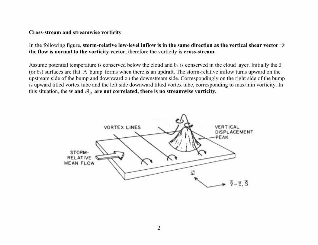
Cross-stream and streamwise vorticity In the following figure, storm-relative low-level inflow is in the same direction as the vertical shear vector the flow is normal to the vorticity vector, therefore the vorticity is cross-stream. Assume potential temperature is conserved below the cloud and e is conserved in the cloud layer. Initially the (or e) surfaces are flat. A 'bump' forms when there is an updraft. The storm-relative inflow turns upward on the upstream side of the bump and downward on the downstream side. Correspondingly on the right side of the bump is upward titled vortex tube and the left side downward tilted vortex tube, corresponding to max/min vorticity. In this situation, the w and H are not correlated, there is no streamwise vorticity.

3

In the next situation, storm-relative flow is normal to the vertical-shear vector, the flow is parallel to the horizontal vorticity vector. In this case, the max w coincides with max H , and w and H are strongly (positively) correlated. There is large streamwise vorticity.

4

The following figure shows the horizontal vorticity H at various points on a hodograph.

5

The Importance of Storm-Relative Flow

Consider the effect of storm motion on the flow as seen by an observer moving along with the storm. Given a particular wind vector V as shown below, for a storm moving with a vector velocity C, the wind in a storm-relative framework can be obtained by subtracting out the storm motion; i.e., we define the relative flow Vr to be V - C.

6

Storm relative wind vectors at different levels on the hodograph:

7

What causes vorticity to be crosswise??

- when storm motion vector lies on hodograph!

In the above example, the hodograph is a straight line and the shear is undirectional (the flow is not unidirectional, however). If the storm-motion vector C

lies on the hodograph, then the storm-relative flow is always parallel to the

shear vector therefore perpendicular to the vorticity vector the vorticity is crosswise. For the above example, if the storm splits into the right and left mover. The storm motion vector for the right mover R

now lies on the right side of the hodograph. In this situation, one gets significant streamwise vorticity.

8

What hodograph causes large streamwise ?

- when C

lies to the right of hodograph!

We see, for example at point 2, that the storm-relative velocity vector 2rV

is essentially parallel to the shear

vorticity vector. When the hodograph is curved, the storm motion is much more likely to lie somewhere off the hodograph. In this case, it can be shown that the simple average of the winds lies somewhere "inside" the curve of the hodograph. Since the advective part of the storm motion usually is considered to arise from the vertically- averaged winds in the storm-bearing layer, such a component of storm motion normally lies off the hodograph when it is curved. A flow which only changes direction with no change in speed (i.e., a hodograph which is a segment of a circle centered on the origin) has only streamwise vorticity.

9

We can compute the component of vorticity in the direction of the storm-relative velocity V C

as

( )| |s

V C VV C

which we call the streamwise vorticity. The numerator,

H = ( )V C V

is known as helicity.

In the case of streamwise vorticity, which is present only when the wind direction changes with height (again, neglecting the contribution from vertical motion's horizontal gradient), one can visualize the flow as being helical; a good mental image is a passed football rotating in a "spiral." Hence, the term helicity is associated directly with streamwise vorticity.

Schematic showing how the superposition of horizontal vorticity (h) parallel to the horizontal flow (Vh) produces a helical flow.

10

Another quantity, called the coefficient of streamwise vorticity,

RH = ( )| || |V C VV C V

is often used too, and it is also called relative helicity. Davies-Jones has shown that the correlation coefficient for storm vertical vorticity and storm vertical velocity is approximately proportional to the environmental relative helicity (calculated based environmental shear and horizontal vorticity). Why large helicity is beneficial for storms? Dough Lilly suggested that the longevity of supercell storms is due to their large helicity. Consider the 3D vorticity equation that we derived earlier:

ˆ( ) ( )V Bkt

If the storm-relative velocity vector V

points in the same direction as the vorticity vector , then

V

= 0, therefore the first term on the right hand side is zero – this term give rises to advection, stretching and tilting terms as we said earlier. When it is zero, the only source of vorticity is the buoyancy production term, which contributes

11

only to the horizontal vorticity, not vertical component of vorticity. In this situation, vertical vorticity is conserved – therefore rotation can be maintained effectively. Thus if a storm becomes a right-mover due to perturbation pressure dynamics, the magnitude of the correlation between w' and s tends to be positive and large, and causes larger streamwise vorticity. The right-mover, from this view point, is also favored for clockwisely curved hodographs - because the storm motion vector of the right mover is further away from the hodograph therefore the storm-relative wind, especially that component that is parallel to the horizontal vorticity, is larger. However, ( )V C V

is not Galilean invariant, i.e., it is dependent on the coordinate system (following the

storm motion) chosen. Therefore there is no single value of helicity for a given sounding (unlike CAPE) – it depends on the value of storm-motion vector C

and requires an estimate of C

before the helicity can be calculated.

It is believed that the storm-relative helicity in the lowest two or three kilometers of the atmosphere is most relevant to the likelihood of supercell behavior with storms in that environment. Therefere, helicity integrated over the lowest 3 km, i.e.,

3

0ˆ( ) ( )

km VH V C k dzz

is often calculated and used as a guidance for thunderstorm forecast. Here we assume the vorticity is given by the environmental wind vector V

. This quantity is called Storm-Relative Environmental Helicity (SREH).

To do that one also has to estimate the storm motion vector C

. A crude way is to use the pressure-weighted mean

wind in the lowest 5 to 6 km.

12

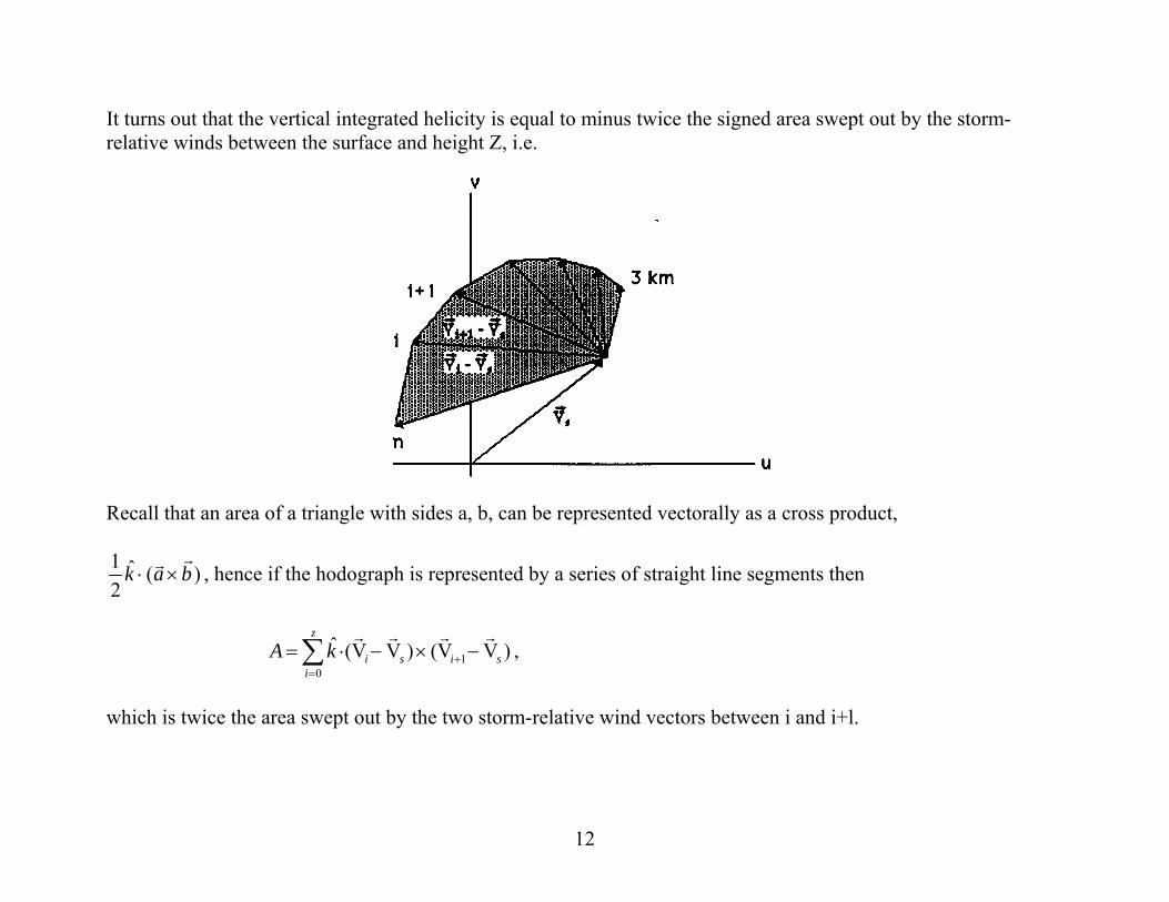
It turns out that the vertical integrated helicity is equal to minus twice the signed area swept out by the storm-relative winds between the surface and height Z, i.e.

Recall that an area of a triangle with sides a, b, can be represented vectorally as a cross product, 1 ˆ ( )2

k a b , hence if the hodograph is represented by a series of straight line segments then

10

ˆ (V V ) (V V )z

i s i si

A k

,

which is twice the area swept out by the two storm-relative wind vectors between i and i+l.

13

Illustration of the area (stippled) swept out by the ground-relative wind vectors along the hodograph from 0 to 3 km. Also shown is the area swept out by the storm-relative wind vectors (hatched).

Therefore, the storm motion can increase or decrease the storm-relative helicity associated with a given hodograph, including change its sign.

Therefore, the farther is the tip of storm-motion vector from the hodograph, usually the larger is the helicity.

14

There are storm motions that can make the storm-relative helicity (averaged over some fixed layer) vanish; one example (there are infinitely many of them) is shown below. Storm motions can lie anywhere on the hodograph, and it is possible to draw contours of storm- relative helicity.

An example of the changes in storm-relative helicity, integrated over the layer from 0 to 3 km, as a function of the storm motion (C). In this example, changes in C are limited to changes in the north-south component, so C moves only upward or downward along the dashed line. There is a point (indicated) where the negative and positive areas cancel and the resulting total storm-relative helicity averaged over the layer vanishes.

15

Because the storm-relative (environmental) helicity depends on how far the storm-motion vector is from the hodograph curve, one can plot 'helicity contours' on a hodograph. It tells us that if the storm-motion vector falls in certain areas on a hodograph, you get certain amount of helicity. The following is an example from Droegemeier et al (1993).

16

Examples of hodographs from environments that produced significant tornado outbreaks in Oklahoma are given below.

Del City Supercell Storm: 0 (m s'l

17

Early results indicate that for tornado producing environment, H ranges from approximately 150 m2 s-2 to upwards of 1000 m2s-2. Davies-Jones (1990) examined the results of 28 tornado cases with the following categories for H (SREH):

150 < H < 299 weak tornadoes 300 < H <449 strong tornadoes H > 450 violent tornado

It is important to point out that helicity will not determine whether or not storms will develop, but instead indicates how a particular storm (or storms) may evolve given the ambient shear. Strongly veering hodograph versus straight hodographs At first glance, tornadic storms would be most likely only when the hodograph shows vertical shear that veers strongly with height, such storms are also possible when the hodograph is relatively straight. Considerable streamwise vorticity may be present with a straight hodograph if storm motions lie significantly to the right of the hodograph. This would occur when split cells move sideways away from the “steering level” flow that originally lies on the straight hodograph. An example of a hodograph which was approximately straight from 2 km to 11 km of altitude, along with the observed storm motions. (L = left-mover, R = right-mover) for a splitting storm pair, are shown below. Also shown are the tracks of splitting storms observed by radar, and the corresponding tracks of storms simulated numerically for similar environmental conditions.

18

Proximity hodograph for the Union City, Oklahoma, splitting storm.

The right mover produced the Union City tornado.

19

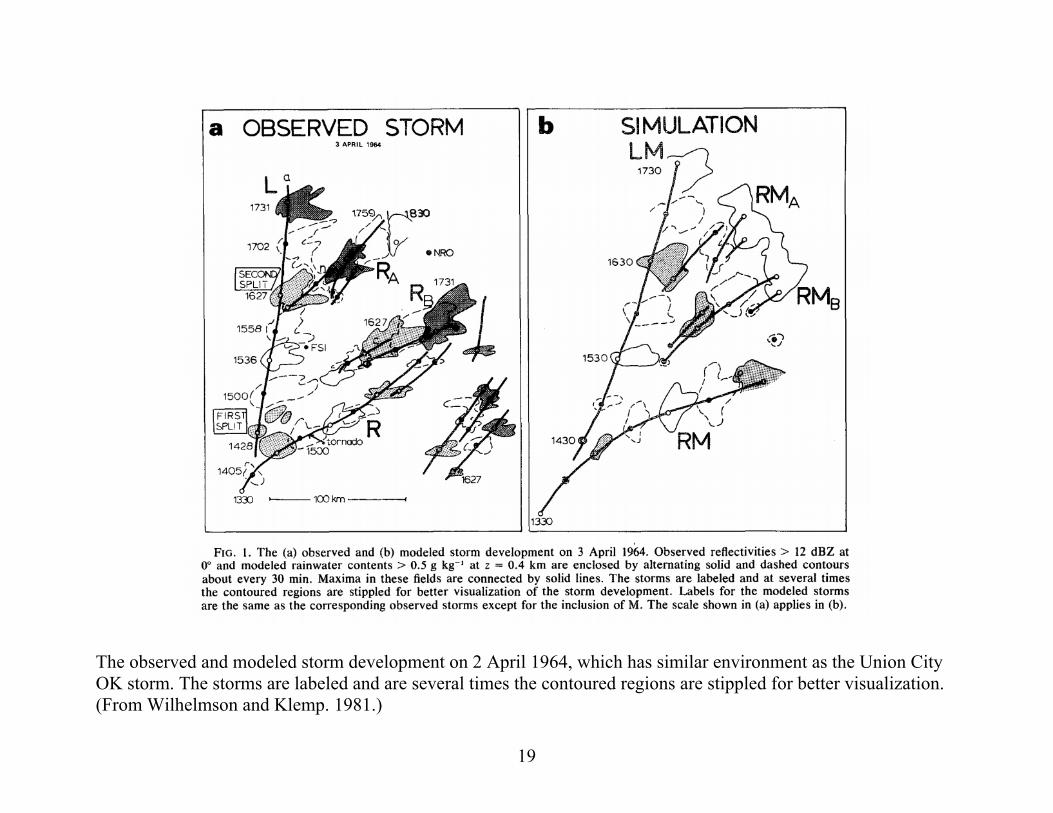
The observed and modeled storm development on 2 April 1964, which has similar environment as the Union City OK storm. The storms are labeled and are several times the contoured regions are stippled for better visualization. (From Wilhelmson and Klemp. 1981.)

20

Summary - Why do we look at helicity?

Given a particular environment, certain aspects of the ambient flow may enhance the energetics and longevity of storms that develop.

Helicity provides yet another method to deduce and/or ascertain information pertaining to the internal

dynamics of severe storms.

Theory suggests the suppression of the inertial energy cascade as a result of the helical nature of a storm.

Helicity is proportional to the low-level streamwise vorticity, and if taken as a storm-relative quantity is proportional to the strength of the low-level storm inflow.

Helicity explicitly accounts for storm motion.

Helicity can be easily calculated from the area on a hodograph diagram.

21

Bulk Richardson Number The quantitative relations between environmental shear and thermal instability and resulting storm type have been studied with numerical models (Weisman and Klemp, 1982; 1984). The results indicate that a parameter known as the bulk Richardson number (BRN), defined by:

21/ 2CAPEBRN

U

is a good predictor of storm type. In the above formula, CAPE is the convective available potential energy (positive area) of the sounding, and

6000 500U u u is a measure of wind shear below 6 km level, and 6000u is the density-weight mean wind in the lowest 6 km layer, and 500u is usually taken as the velocity at 500m above ground (Weisman and Klemp, 1982). According to Weisman and Klemp,

When BRN 40, storms are likely to be multicell, and When BRN 40, storms may be supercell When BRN < 10 with unidirectional shear, storms may be suppressed by the excessive shear, although with

curved hodographs this suppression is less noticeable. It should be noted that a shortage of CAPE in a sounding may be overcome if mesoscale or synoptic scale dynamical lifting is sufficiently strong. However, a shortage of shear (equivalent to weak low-level storm inflow) or an unfavorable hodograph shape are much more difficult to compensate for.

22

23

Summary – Roles of shear and CAPE

Strong vertical shear and a veering or straight hodograph in an environment of veering winds are important in setting the stage for supercell convection and possible tornadoes.

Large CAPE is also desirable, although this requirement may be relaxed if strong lifting is present. Absence of shear, however, is an obstacle to supercell development that is more difficult to overcome. Nevertheless, hodograph structure is very sensitive to changes in the wind field, and many mesoscale regions

of favorable shear are never sampled by the existing rawinsonde network.

It is therefore imperative that the forecaster use all available data - surface obs, upper air obs, wind profilers, radar data and satellite images – in assessing the risks of severe weather in the thunderstorm season.

Reference: Davies-Jones, R. P., 1984: Streamwise vorticity: the origin of updraft rotation in supercell storms. J. Atmos. Sci..

41, 2991-3006. Davies-Jones, R.P., D. Burgess, and M. Foster, 1990: Helicity as a tornado forecast parameter. Preprints, 16th

Conf. on Severe Local Storms, 588-592. Droegemeier, K. K., S. M. Lazarus, and R. P. Davies-Jones, 1993: The influence of helicity on numerically

simulated convective storms. Mon. Wea. Rev., 121, 2005-2029. Lilly, D. K., 1986: The structure, energetics and propagation of rotating convective storms. Part II: helicity and

storm stabilization. J. Atmos. Sci.. 43. 126-140. Weisman, M. L., and J. B. Klemp, 1982: The dependence of numerically simulated convective storms on vertical

shear and buoyancy. Mon. Wea. Rev.. 110. 504-520. Weisman, M.L., and J. B. Klemp, 1984: The structure and classification of numerically simulated convective

storms in directionally varying shears. Mon. Wea. Rev., 112, 2479-2498.