Genomics and High Throughput Sequencing Technologies: Applications

Introduction to transcriptome analysis using high-
throughput sequencing technologies
D. Puthier 2015

Main objectives of transcriptome analysis● Understand the molecular mechanisms
underlying gene expression○ Interplay between regulatory elements and
expression■ Create regulatory model
● E.g; to assess the impact of altered variant or epigenetic landscape on gene expression
● Classification of samples (e.g tumors)○ Class discovery○ Class prediction
Relies on a holistic view of the system

Some players of the RNA world
● Messenger RNA (mRNA)○ Protein coding○ Polyadenylated○ 1-5% of total RNA
● Ribosomal RNA (rRNA)○ 4 types in eukaryotes (18s, 28s, 5.8s, 5s)○ 80-90% of total RNA
● Transfert RNA○ 15% of total RNA

Some players of the RNA world
● miRNA○ Regulatory RNA (mostly through binding of 3’
UTR target genes )● SnRNA
○ Uridine-rich○ Several are related to splicing mechanism○ Some are found in the nucleolus (snoRNA)
■ Related to rRNA biogenesis● eRNA
○ Enhancer RNA● And many others...
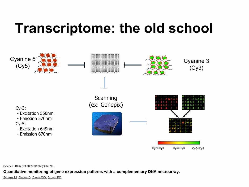
Transcriptome: the old school
Cyanine 5 (Cy5)
Cyanine 3 (Cy3)
Scanning(ex: Genepix)
Cy-3: - Excitation 550nm - Emission 570nmCy-5: - Excitation 649nm - Emission 670nm

Transcriptome still the old school
● Principle:○ In situ synthesis of
oligonucleotides○ Features
■ Cells: 24µm x 24µm■ ~107 oligos per cell■ ~ 4.105-1,5.106 probes
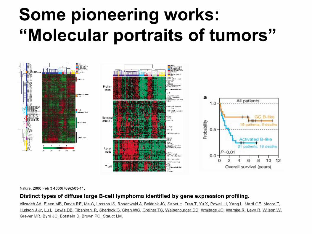
Some pioneering works: “Molecular portraits of tumors”

Some pioneering works: Cluster analysis to infer gene function

Some pioneering work: tumor class prediction
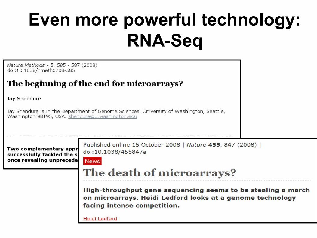
Even more powerful technology:RNA-Seq
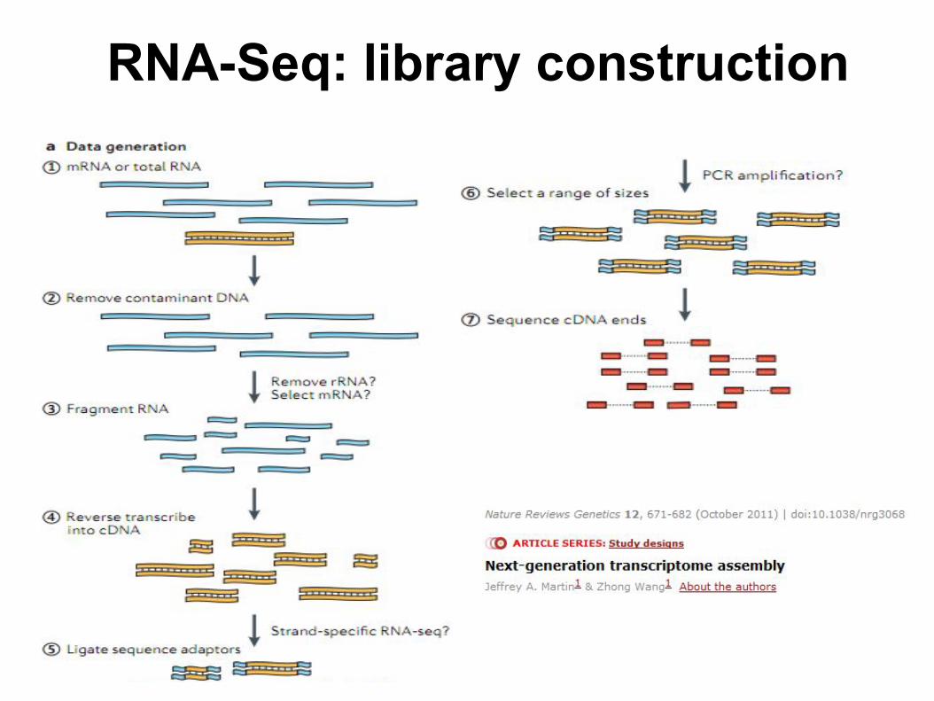
RNA-Seq: library construction
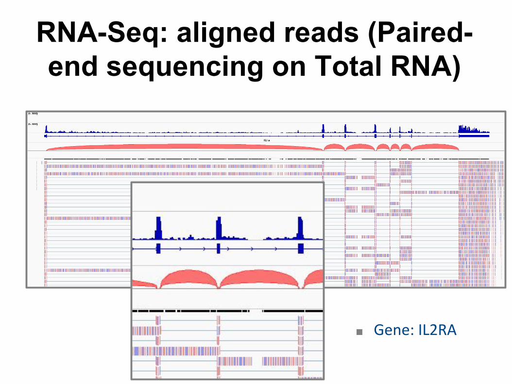
RNA-Seq: aligned reads (Paired-end sequencing on Total RNA)
■ Gene: IL2RA
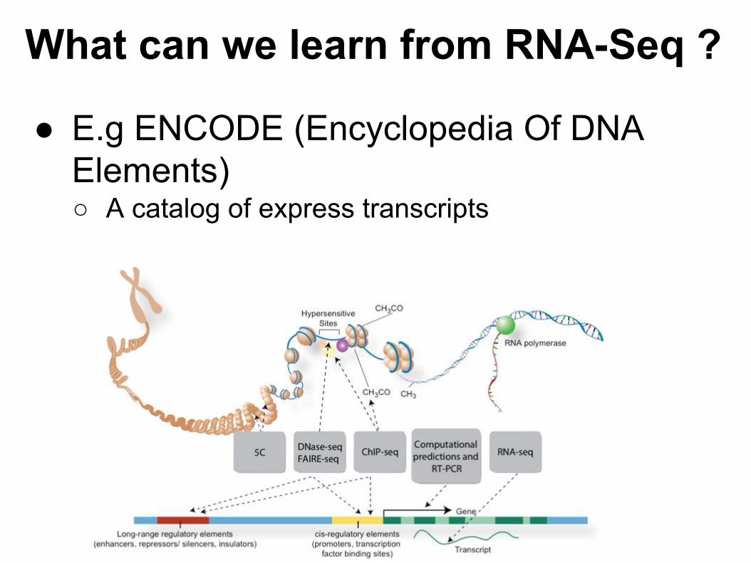
● E.g ENCODE (Encyclopedia Of DNA Elements)○ A catalog of express transcripts
What can we learn from RNA-Seq ?

Some key results of ENCODE analysis
● 15 cell lines studied○ RNA-Seq, CAGE-Seq, RNA-PET○ Long RNA-Seq (76) vs short (36)○ Subnuclear compartments
■ chromatin, nucleoplasm and nucleoli
● Human genome coverage by transcripts○ 62.1% covered by processed transcripts○ 74.7 % covered by primary transcripts, ○ Significant reduction of ”intergenic regions”○ 10–12 expressed isoforms per gene per cell line
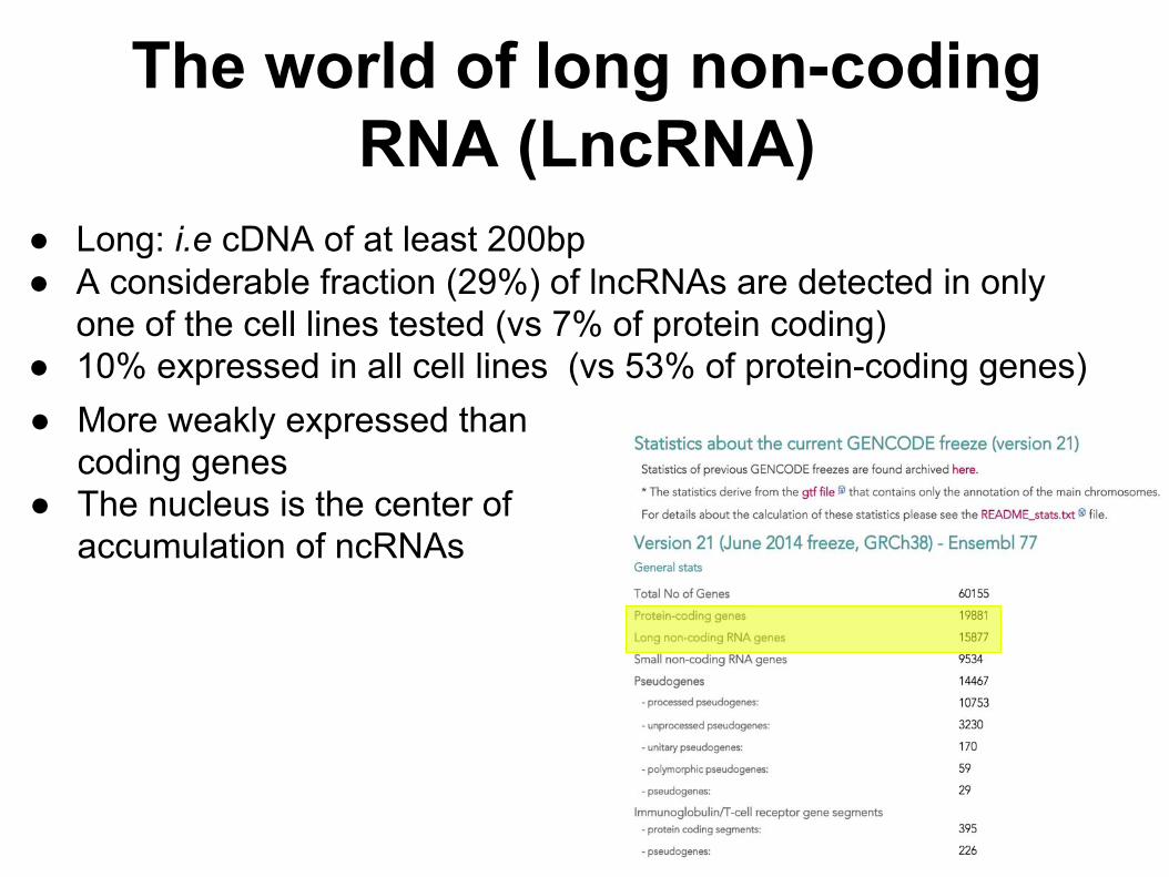
The world of long non-coding RNA (LncRNA)
● Long: i.e cDNA of at least 200bp ● A considerable fraction (29%) of lncRNAs are detected in only
one of the cell lines tested (vs 7% of protein coding)● 10% expressed in all cell lines (vs 53% of protein-coding genes)● More weakly expressed than
coding genes● The nucleus is the center of
accumulation of ncRNAs
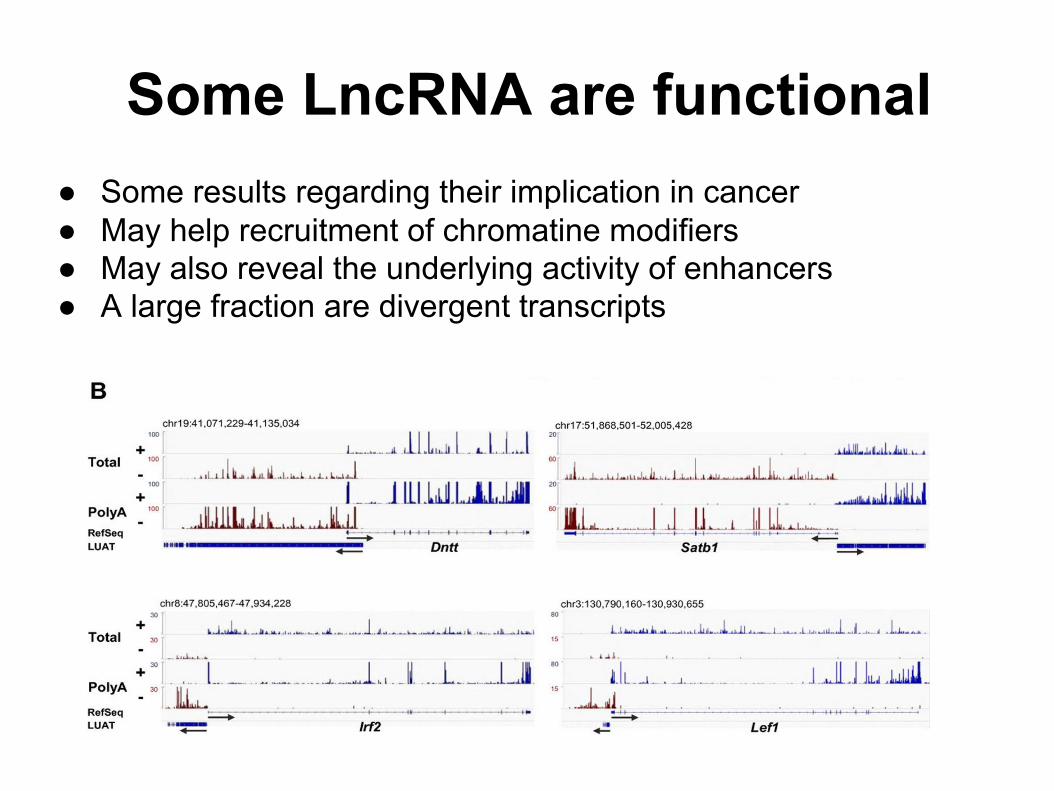
● Some results regarding their implication in cancer● May help recruitment of chromatine modifiers● May also reveal the underlying activity of enhancers● A large fraction are divergent transcripts
Some LncRNA are functional

● Fragmentation methods○ RNA: nebulization, magnesium-catalyzed
hydrolysis, enzymatic clivage (RNAse III)○ cDNA: sonication, Dnase I treatment
● Depletion of highly abundant transcripts○ Ribosomal RNA (rRNA)
■ Positive selection of mRNA . Poly(A) selection.■ Negative selection. (RiboMinusTM)
● Select also pre-messenger
● Strand specificity● Single-end or Paired-end sequencing
http://www.bioconductor.org/help/course-materials/2009/EMBLJune09/Talks/RNAseq-Paul.pdf
RNA-Seq: protocol variations

Strand specific RNA-Seq
● Most kits are now strand-specific○ Better estimation of gene expression level.○ Better reconstruction of transcript model.
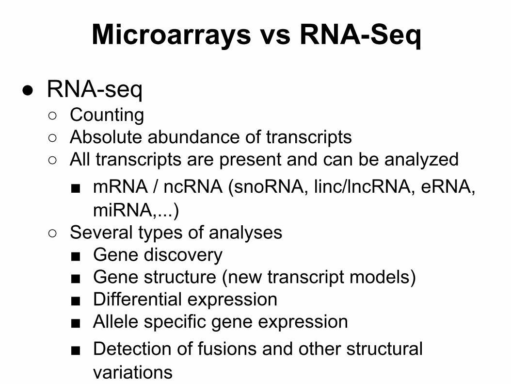
● RNA-seq○ Counting○ Absolute abundance of transcripts○ All transcripts are present and can be analyzed
■ mRNA / ncRNA (snoRNA, linc/lncRNA, eRNA,miRNA,...)
○ Several types of analyses■ Gene discovery■ Gene structure (new transcript models)■ Differential expression■ Allele specific gene expression■ Detection of fusions and other structural
variations
...
Microarrays vs RNA-Seq

Microarrays vs RNA-Seq
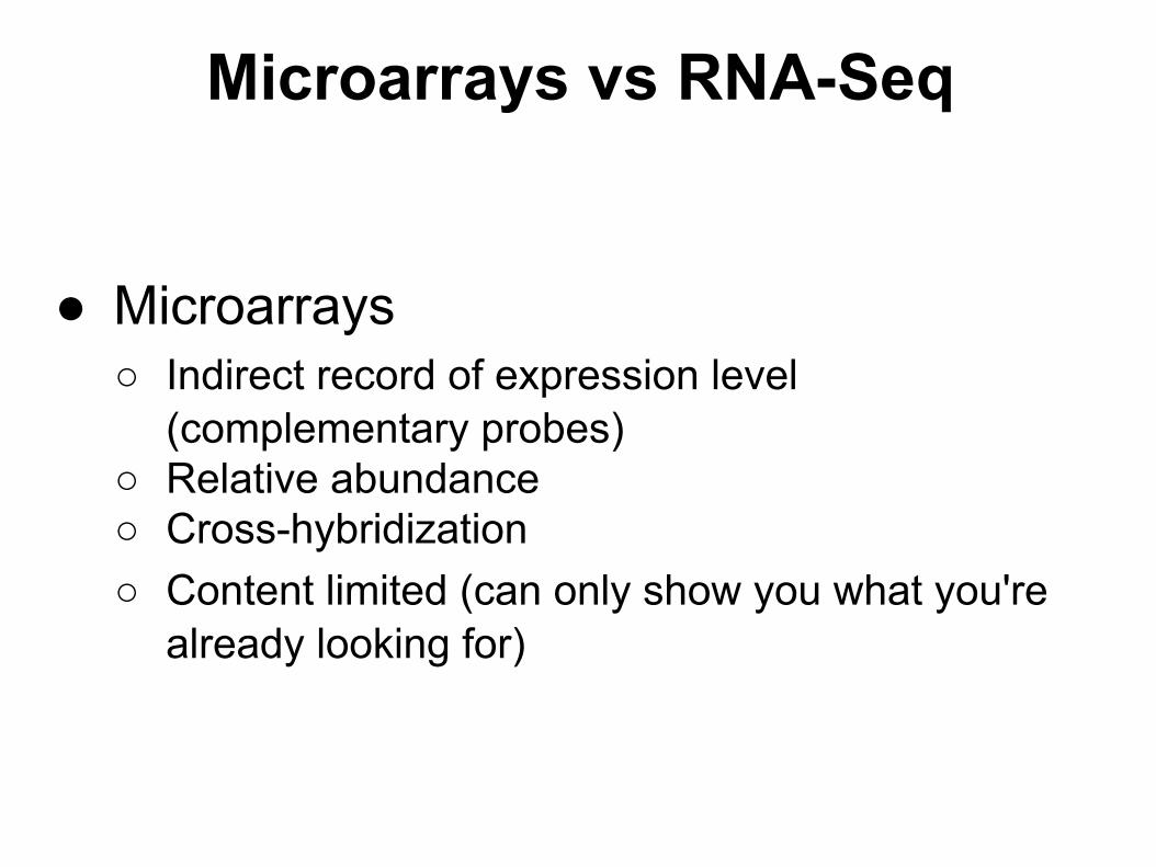
● Microarrays○ Indirect record of expression level
(complementary probes)○ Relative abundance○ Cross-hybridization○ Content limited (can only show you what you're
already looking for)
Microarrays vs RNA-Seq

High reproducibility and dynamic range
(a) Comparison of two brain technical replicate RNA-Seq determinations for all mouse gene models (from the UCSC genome database), measured in reads per kilobase of exon per million mapped sequence reads (RPKM), which is a normalized measure of exonic read density; R2 = 0.96.
(c) Six in vitro–synthesized reference transcripts of lengths 0.3–10 kb were added to the liver RNA sample (1.2 104 to 1.2 109 transcripts per sample; R2 > 0.99).
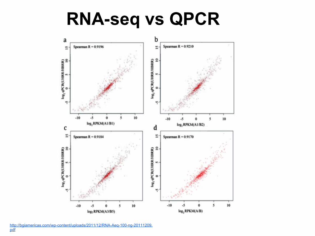
RNA-seq vs QPCR
http://bgiamericas.com/wp-content/uploads/2011/12/RNA-Aeq-100-ng-20111209.pdf

Some RNA-Seq drawbacks
● Current disadvantages○ More time consuming than any microarray
technology○ Some (lots of) data analysis issues
■ Mapping reads to splice junctions■ Computing accurate transcript models■ Contribution of high-abundance RNAs (eg
ribosomal) could dilute the remaining transcript population; sequencing depth is important
http://www.bioconductor.org/help/course-materials/2009/EMBLJune09/Talks/RNAseq-Paul.pdf

Do arrays and RNA-Seq tell a consistent story?
● Do arrays and RNA-Seq tell a consistent story?○ ”The relationship is not quite linear … but the vast majority of the
expression values are similar between the methods. Scatter increases at low expression … as background correction methods for arrays are complicated when signal levels approach noise levels. Similarly, RNA-Seq is a sampling method and stochastic events become a source of error in the quantification of rare transcripts ”
○ ”Given the substantial agreement between the two methods, the array data in the literature should be durable”
Comparison of array and RNA-Seq data for measuring differential gene expression in the heads of male and female D. pseudoobscura

Raw data: the fastq file format■ Header
■ Sequence
■ + (optional header)
■ Quality (default Sanger-style)
@QSEQ32.249996 HWUSI-EAS1691:3:1:17036:13000#0/1 PF=0 length=36GGGGGTCATCATCATTTGATCTGGGAAAGGCTACTG+=.+5:<<<<>AA?0A>;A*A################@QSEQ32.249997 HWUSI-EAS1691:3:1:17257:12994#0/1 PF=1 length=36TGTACAACAACAACCTGAATGGCATACTGGTTGCTG+DDDD<BDBDB??BB*DD:D#################

Sanger quality score
● Sanger quality score (Phred quality score): Measure the quality of each base call○ Based on p, the probality of error (the probability that the
corresponding base call is incorrect)○ Qsanger= -10*log10(p)○ p = 0.01 <=> Qsanger 20
● Quality score are in ASCII 33 ● Note that SRA has adopted Sanger quality score although
original fastq files may use different quality score (see: http://en.wikipedia.org/wiki/FASTQ_format)
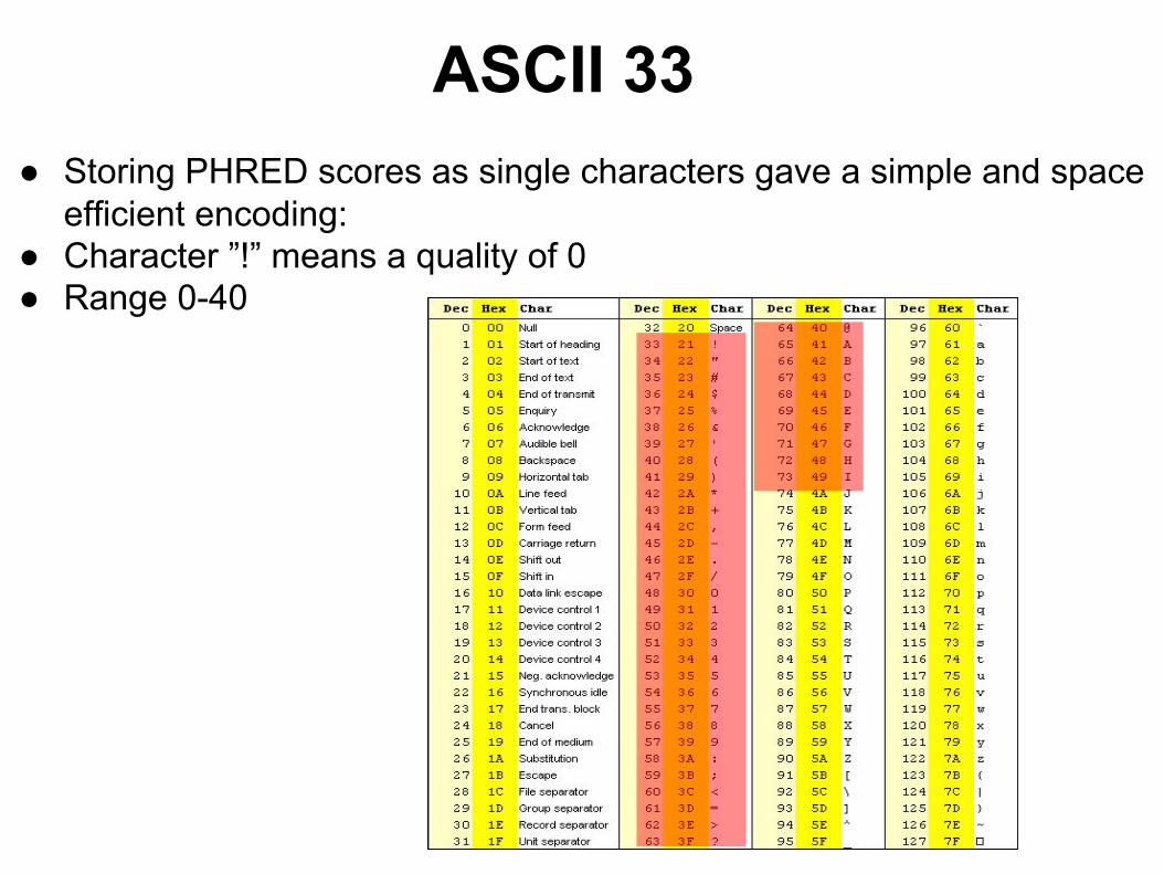
ASCII 33● Storing PHRED scores as single characters gave a simple and space
efficient encoding:● Character ”!” means a quality of 0● Range 0-40

Quality control for high throughput sequence data
● First step of analysis ○ Quality control○ Trimming
■ Ensure proper quality of selected reads.■ The importance of this step depends on the
aligner used in downstream analysis

Quality control with FastQC
Quality
Position in read
Nb Reads
Mean Phred Score
Position in read
Look also at over-represented sequences

Reference mapping and de novo assembly
● Downstream approaches depend on the availability of a reference genome○ If reference :
■ Align the read to that reference● Rather straightforward
○ If no reference■ Perform read assembly (contigs) and compare
them to known RNA sequences (e.g blast).● More complex approaches.

Bowtie a very popular aligner
● Burrows Wheeler Transform-based algorithm● Two phases: “seed and extend”.● The Burrows-Wheeler Transform of a text T, BWT(T), can be
constructed as follows. ○ The character $ is appended to T, where $ is a character not
in T that is lexicographically less than all characters in T. ○ The Burrows-Wheeler Matrix of T, BWM(T), is obtained by
computing the matrix whose rows comprise all cyclic rotations of T sorted lexicographically.
1234567
acaacg$caacg$aaacg$acacg$acacg$acaag$acaac$acaacg
acaacg$
$acaacgaacg$acacaacg$acg$acacaacg$acg$acaag$acaac
T BWT (T)
gc$aaac
7314256

● Burrows-Wheeler Matrices have a property called the Last First (LF) Mapping. ○ The ith occurrence of character c in the last column
corresponds to the same text character as the ith occurrence of c in the first column
○ Example: searching ”AAC” in ACAACG
● Second phase is “extension”
Bowtie principle
7314256

Mappability issues● Mappability: sequence uniqueness of the reference● These tracks display the level of sequence uniqueness of the
reference NCBI36/hg18 genome assembly. They were generated using different window sizes, and high signal will be found in areas where the sequence is unique.
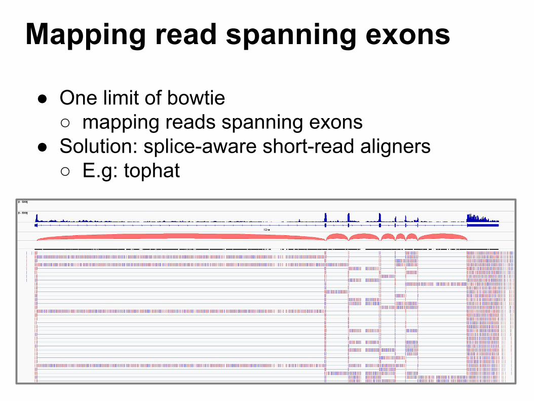
Mapping read spanning exons
● One limit of bowtie ○ mapping reads spanning exons
● Solution: splice-aware short-read aligners○ E.g: tophat

Searching for novel transcript model: cufflinks
Read pair
Gapped alignment

Quantification
● Objective○ Count the number of reads that fall in each gene
■ HTSeq-count, featureCounts,...● Known issue
○ Positive association between gene counts and length■ suggests higher expression among longer
genes

RPKM / FPKM● Transcrits of different length have different read count
● Tag count is normalized for transcrit length and total read number in the measurement (RPKM, Reads Per Kilobase of exon model per Million mapped reads)
● 1 RPKM corresponds to approximately one transcript per cell● FPKM, Fragments Per Kilobase of exon model per Million
mapped reads (paired-end sequencing)
Some proposed normalization methods
● Reads Per Kilobase per Million mapped reads (RPKM): This approach was initially introduced to facilitate comparisons between genes within a sample.○ Not sufficient
● Upper Quartile (UQ): the total counts are replaced by the upper quartile of counts different from 0 in the computation of the normalization factors.
● Trimmed Mean of M-values (TMM): This normalization method is implemented in the edgeR Bioconductor package (version 2.4.0). Scaling is based on a subset of M values○ TMM seems to provide a robust scaling factor.

Next step ?
● Compare various samples○ Eg.
■ control vs treated■ Normal vs tumor■ Poor/bad prognosis■ …
○ Compare expression level, isoforms, fusions,...● Perform classification● Compare RNA-Seq data to regulatory
data (ChIP-Seq,...)

Sequence read Archive (SRA)
● The SRA archives high-throughput sequencing data that are associated with:
● RNA-Seq, ChIP-Seq, and epigenomic data that are submitted to GEO

SRA growth

Merci