Three Roles for Statistical Significance and the Validity Frontier in Theory Testing

Allen S. Lee Virginia Commonwealth University

allenslee@alum.mit.edu

Kaveh Mohajeri Lund University

kaveh.mohajeri@ics.lu.se

Geoffrey S. Hubona R-Courseware.com

ghubona@gmail.com

Abstract

This study offers a method for empirically testing theories operationalized in the form of multivariate statistical models. An innovation of the method is that it distinguishes testing into three separate forms, “effect testing,” “prediction testing,” and “theory testing,” where statistical significance plays a separate role in each one. In another innovation, the researcher specifies not only his or her desired level of statistical significance, but also his or her desired level of practical significance. Statistical significance and practical significance each serve as a dimension in a two-dimensional table that specifies the rejection region – the region where the researcher can justify the decision to reject the theory being tested. The boundary of the rejection region is the “validity frontier,” which ongoing research may advance so as to reduce the size of the rejection region. 1. Introduction

What are the roles of statistical significance in theory testing?

Consider the situation where a behavioral theory in information systems (IS) is operationalized mathematically as a set of one or more equations. Typically, the left-hand side of an equation is a dependent variable and the right-hand side is often a linear combination of independent variables, but nonlinear combinations are certainly allowed too. The set of equations is then fitted to a population with a sample of data taken from the population. Traditionally, hypothesis testing is conducted to determine the level of statistical significance of the estimated coefficients of the independent variables.

The purpose of this essay is to innovate two additional roles for statistical significance in testing: In addition to the role played by statistical significance in the traditional hypothesis testing just described, we propose a second role for statistical significance in prediction testing (the testing of an individual prediction made by the theory’s equations after they are fitted with

sample data to a population) and a third role for statistical significance in theory testing (the testing of the theory through the multiple predictions it makes).

In the second and next section of this essay, we will use a case from natural science to introduce some basic ideas that we will subsequently refine with a behavioral IS example. The reason for using a natural-science case is that its subject matter, being physical and unambiguous, is conducive to the introduction of more abstract ideas without unnecessary complications.

This introductory case will allow us, in the third section, to make a revealing examination of behavioral-science theorizing which involves statistical inference. We will draw attention to how traditional statistical hypothesis testing for the statistical significance of estimated coefficients, while not incorrect, is incomplete when it comes to the matter of theory testing. We will show how to conduct statistical behavioral research so as to carry out, to completion, the required scientific method of testing. Then, in the fourth section, we will introduce a new methodological concept, a theory’s “validity frontier,” which is a visual way of summarizing how well a behavioral theory does, or does not, predict and therefore is, or is not, valid. It accounts for a researcher’s own preferences for how inaccurate a theory’s predictions may be until the researcher himself or herself feels compelled to consider the theory to fail. 2. A natural-science example: an illustration of the use of statistical inference in theorizing

For an illustration of the use of statistical inference in natural science, we turn to an example of an object falling in a liquid for which 19 data points are collected, where each data point denotes the object’s velocity V (measured in meters/second or m/s) as the independent variable and the object’s force F (measured in Newtons or N) as the dependent variable.

The source of the material in Figure 1 is [14]. The original data for the 19 data points (the measured values) and the two graphs are taken from the downloaded

5737

Proceedings of the 50th Hawaii International Conference on System Sciences | 2017

URI: http://hdl.handle.net/10125/41854ISBN: 978-0-9981331-0-2CC-BY-NC-ND

documents. The “Prediction Error” columns have been added.

As the left-hand side of Figure 1 indicates for the 19 data points, a simple regression explains the force F of the falling object as a linear function of the object’s velocity, “F = -0.4612V + 5.6518,” where the explanation is excellent statistically. The p-value for the estimated coefficient -0.4612 is almost as small as 0 (which would ideally be its best value) and the R2 value is 0.9698 (where ideally its best value would be 1). In behavioral research, numerical values for the p-value and the R2 are rarely, if ever, as good as these, which would be regarded as excellent support for the theoretical explanation being tested.

However, as the right-hand side of Figure 1 indicates, the very same 19 data points also allow a different regression to explain the same force F of the falling object as a nonlinear (quadratic) function of the

object’s velocity, “F = -0.0271V2 -0.1278V + 4.977,” where the explanation is even better than the prior one. The p-value for the estimated coefficient -0.0271 and the p-value for the other estimated coefficient -0.1278 are both excellent (each is almost as small as 0) and the value for the R2, as 0.9986, is even closer to 1 than the R2 for the linear equation.

Scientifically, the bottom-line criterion is not so much one or another statistical measure, but a predictive measure: Which theoretical explanation is more predictive? In Figure 1, there are two “Prediction Error” columns; the column for the linear explanation, “F = -0.4612V + 5.6518,” shows prediction errors that are consistently greater than the prediction errors in the same rows in the column for the other explanation, “F = -0.0271V2 -0.1278V + 4.977.” The better predictive power is sufficient to reject the former explanation in favor of the latter one.

Figure 1

5738

Four additional points are worth noting. The first one is that statistical measures (such as the R2 value, and the estimated coefficient’s p-value or level of statistical significance) are indeed helpful to show how well a general equation (such as “F = ß0 + ß1V” or “F = ß0 + ß1V + ß2V2”), when applied to a set of data sampled from a population, fits the population; however, in general, statistical measures and statistical inference play an ancillary role (or, at best, a supporting role) in science. In our example, how well or poorly an equation statistically fits the population is a matter that precedes, and is different from, how well the equation predicts. Individual predictions must still be made from the equation, and then empirically tested to see if each one succeeds or fails. Thus, empirically testing a theory through its predictions follows, and is not pre-empted or supplanted by, any statistical tasks of fitting the theory’s equation(s) to a population. Historically speaking, statistical inference is just one possible, but not necessary, research tool available to scientific research. Consider that Neyman and Egon Pearson introduced the idea of a confidence interval only in 1928 and the procedure for hypothesis testing only in 1933 [1]. If research must be statistical to be scientific, then this would mean that there was no science before 1928. Also, statistical hypothesis testing of the estimated coefficient of an independent variable (e.g., “H0: ß1 = 0” regarding “F = ß0 + ß1V + ß2V2”) is not to be confused with the empirical testing that compares predicted values with observed values (e.g., comparing a value predicted for F with the value observed for F after “F = ß0 + ß1V + ß2V2” has been fitted to the population where the empirical testing is being conducted).

The second additional point worth noting is that even an incorrect theory can have excellent statistical measurements. As even a first-year university physics student knows, the linear equation “F = -0.4612V + 5.6518” (or actually, regarding our example of the object falling in a liquid, any linear equation) is scientifically incorrect, despite its having an excellent p-value for an estimated coefficient and an excellent R2 value. And if this is the case in natural science, then what does this portend for the case in social science, where typically p-values and R2 values are hardly ever as good as they are even in the incorrect natural science case of “F = -0.4612V + 5.6518”? The lesson is that, because excellent statistical results – e.g., even an astonishing R2 of 0.9698 and even estimated coefficients with high statistical significance – can still be consistent with an incorrect theory, the scientific status of a theory as true (or, at least, as not rejected) does not follow from the quality of its statistical fit (assuming that statistical inference is used at all), but from the empirical testing of the predictions made from it.

The third point is that, in our example of the object falling in a liquid, we can conduct a test of either theory (one theory being that force and velocity are related to each other by the relation “F = ß0 + ß1V” and the other theory being that the relation is instead “F = ß0 + ß1V + ß2V2) by noting how many of its predictions can be regarded to succeed or fail. Of course, this would involve establishing a threshold level for how great a prediction error may be before the prediction is judged to fail, as well as establishing another threshold level for how many predictions may fail before the theory itself is also judged to fail. Both thresholds, we will explain in detail below, involve a role for statistical significance – but they are roles different from the one associated with the traditional testing of the null hypothesis pertaining to an estimated coefficient, e.g., “H0: ß1 = 0.”

The fourth point is that, in the literature of behavioral IS articles, numerous studies conducted by prominent researchers and published in prominent journals demonstrate the practice of engaging in traditional statistical hypothesis testing with regard to estimated coefficients, but these studies never proceed to the subsequent, necessary scientific step of empirically testing a theory by computing any values it predicts for a dependent variable and then comparing them to values observed for the dependent variable. Such studies include [2], [3], [4], [5], [6], [7], [8], [9], [10], [11]. All of these studies mention “prediction,” “predictor,” “predicting,” or “predict,” but not one of them describes or reports the actual test of any prediction. The journals in which these studies appear include all eight of the “Senior Scholars’ Basket of Journals.” The statistical method in these studies is not incorrect, but is incomplete in so far as the theories being advanced were not empirically tested. In the next section, we propose a remedy for this situation. 3. In behavioral IS research: a remedy for making the use of statistical inference complete for theory testing

Testing a theory, where the researcher has used a sample of data from a population to fit the theory to the population, is not as simple as using the fitted theory to make and test just a single prediction. The main reason for this is that sampling error, introduced whenever a sample of data is taken from a population, can induce inaccuracies in the fitted equation’s coefficients. For instance, in an example from Figure 1, the coefficient -0.1278 in “F = -0.0271V2 -0.1278V + 4.977” could be different from what the true value of it is. (In statistical parlance, the equivalent statement would be that the estimated value ß̂2 is different from the true, but known, value ß2, where the predicted value of F should ideally

5739

be computed using ß2, not ß̂2.) This, in turn, creates the complication that the result of testing a predicted value of F could then be disputed because the predicted value of F is itself inaccurate, whether the result is “the prediction succeeds” or “the prediction fails.”

The remedy to this problem involves two actions. One is to make the decision that a prediction fails only if the difference between the predicted value and the observed value reaches a given threshold level, where this threshold level is to be determined. The second action is to make the decision that the theory fails not if just one prediction fails, but only if the number of predictions that fail, out of the total number of predictions that are tested, also reaches a given threshold level, where this threshold level is also to be determined. How are the two threshold levels to be determined?

3.1. Determining the threshold level for where a prediction fails

One approach to determining the threshold level for where a prediction fails is for the researcher to rely on his or her own judgment in a reasoned, and replicable, manner. The use of a critical level of statistical significance, such as “reject H0 where α = .05,” establishes the precedent allowing this to be done. Just as a researcher is allowed to determine the threshold level of statistical significance in hypothesis testing to be a numerical value that the researcher chooses for α (the threshold level beyond which the measured p-value allows the researcher to make the decision to reject H0), we regard a researcher as no less allowed to determine the threshold level of prediction error beyond which the observed or measured prediction error allows the researcher to make the decision that the prediction fails. Just as the threshold level in statistical hypothesis testing is denoted with the symbol α, we choose to denote as the threshold level in prediction testing with the symbol π. And just as a researcher can conduct “what if” analyses with different values of α, showing how sensitive or insensitive the conclusion (i.e., “reject the null hypothesis”) is to different values of α, the researcher can also conduct “what if” analyses with different values of π, showing how sensitive or insensitive the conclusion (e.g., “the prediction fails”) is to different values of π.

We choose, furthermore, to take advantage of a particular circumstance in behavioral information systems research. It is that many or most variables are measured on a Likert scale, typically from 1 to 7. Suppose that a dependent variable (such as “the individual’s behavioral intention to use the given technology”) is measured on a scale from 1 to 7, that a numerical value is predicted for the dependent variable,

and that the resulting prediction error turns out to be just ±0.1 unit (on the same scale from 1 to 7). On the one hand, a researcher may consider this prediction error to be so small as to lack practical significance; the researcher considers it to be insufficient to judge the prediction to fail and instead writes it off as an artifact of sampling error. On the other hand, if ±0.1 unit on a scale from 1 to 7 is too small to bear any practical significance, then how large must a prediction error be to provide sufficient confidence to a researcher to make the decision that the prediction has failed? Consider prediction errors that cross the threshold of ±1.0 unit. Such a threshold would be particularly generous, considering that it spans a range of 2 units and therefore covers 33% of the entire scale.

Analogously to statistical hypothesis testing, just as a researcher may choose his or her desired level of “statistical significance,” α, to be a particular numerical value such as .05, a researcher may also choose what we are now naming his or her desired level of “practical significance,” π, as being ±1.0 unit for the given variable operationalized on a Likert scale from 1 to 7. And just as it would behoove the researcher to see if his or her conclusions change or are insensitive to changes in the value chosen for α, it would behoove the researcher to see if his or her conclusions change or are insensitive to changes in the value chosen for π. The larger the range of values across which the conclusion remains unchanged, the more durable or objective the conclusion would be; just as this has always been the case regarding the range of values for α, this is also the case regarding the range of values for π.

An additional necessary consideration is the probability, in decision making, of a false positive. In statistical hypothesis testing, it is the probability, where the null hypothesis H0 actually happens to be true, that the researcher makes the decision to reject it. In fact, this is the definition of, and is denoted as, the aforementioned α. It is the probability of making the decision that the independent variable, whose estimated coefficient’s statistical significance is being measured, is indeed related to the dependent variable when, in actuality, it is not (hence, “false positive”). Analogously, in prediction testing, it is the probability of making the decision that there exists a difference between the predicted value and the observed or measured value (apart from the “noise” of sampling-induced inaccuracy in computing the prediction) when, in actuality, there is no such difference. Unfortunately, to denote the latter probability, the symbol α is already taken. Therefore, to denote the two probabilities, we will distinguish them as αet and αpt. For the former, αet, the subscript “et” refers to effect testing, insofar as statistical hypothesis testing with regard to the null hypothesis “H0: ßi = 0” is about whether or not the

5740

coefficient ßi of the independent variable in a multivariate analysis indeed indicates an effect on the dependent variable. (Our usage of the term “effect” here is consistent with the term “effect size.”) For the latter, αpt, the subscript “pt” refers to prediction testing. By convention, the maximum acceptable probability or threshold level for making the decision error of a false positive is 0.05.

What this means is that, in the test of a prediction made by the theory (which is that there is no difference between the predicted value and the observed or measured value, apart from the “noise” of sampling-induced inaccuracy in computing the prediction), the researcher is willing to accept up to a 5% probability that he or she would be incorrectly deciding, whenever the prediction error exceeds the numerical value that he or she earlier established for π (such as ±1.0), that the difference exists – i.e., that the prediction fails and therefore contradicts the theory.

3.2. Determining the threshold level for where a theory fails

As mentioned, the reason why a single prediction is

not sufficient to test the theory making the prediction is that sampling error induces “noise” in the computation of the value that is predicted. Suppose, then, 100 predictions are tested instead of just 1. If 90 of the 100 fail, the researcher could be confident in rejecting the theory making the predictions. But suppose just 10 of the 100 predictions fail. In this case, would the researcher have sufficient confidence to reject the theory? After all, some of the predictions deemed to fail could be false positives. The binomial distribution provides a formula by which to compute the probability that, out of n trials, x of them will be successes (as well as, therefore, the probability that x or more of them will be successes), where the probability of success in a given trial is p. In our application of the binomial formula, (1) a false positive is defined as a “success,” which is the occurrence of a prediction that is deemed to fail because its prediction error exceeds π, when in fact the prediction is successful, (2) n = 100, (3) x = 10, and (4) the researcher chooses 0.05 as the value for the probability p (which in this application of the binomial is also the probability of a false positive αpt). Thus the probability of making the decision that 10 or more of the 100 predictions fail, when in fact the predictions are true, can be computed from the cumulative binomial formula as only 0.028, or 2.8%. Because this probability fits the definition of a p-value, this implies that the theory can be rejected at a critical significance level of 0.05; we designate this latest critical significance level as αtt, where the subscript “tt” refers

to theory testing. Like αet and αpt, we note αtt is the probability of a false positive – here, the probability of making the decision that the independent and dependent variables in the theory are related to each other as the theorized equation specifies, when they are in fact not so related – where convention regarding false positives dictates that this threshold level not be greater than 0.05.

Because the p-value of 0.028 crosses the threshold level of αtt as 0.05, the researcher may properly reject the theory as true. Equivalently, the researcher may reject, at the 97.2% level of confidence, the statement that the theory is true when the researcher judges 10 of the predictions to fail, where a failed prediction is one where the prediction error exceeds the threshold of the numerical value that the researcher earlier assigned to π (such as ±1.0).

To recapitulate our discussion from the beginning of

the essay, we have formulated a research method by which not only (1) a theory, operationalized in the form of an equation, is statistically fitted to a population with data sampled from the population in a process that makes use of statistical significance in the traditional form which we denote as αet, but also (2) the same theory is then empirically tested through the predictions it makes, making use of statistical significance in our newly innovated forms of αpt and αtt. As noted earlier, numerous behavioral studies in information systems, conducted by prominent researchers and published in prominent journals, demonstrate the practice of engaging in traditional statistical hypothesis testing with regard to estimated coefficients (i.e., the phrase just designated as “(1)”), but these studies never proceed to the subsequent, necessary scientific step of empirically testing a theory by computing any values it predicts for a dependent variable and then comparing them to values observed for the dependent variable (i.e., the phrase just designated as “(2)”). In this study, we are contributing “(2).” 4. An application of the three roles of statistical significance and a theory’s validity frontier

We were fortunate enough for Lee and Hubona [12] to grant us access to the same data set that they used in Appendix C of their article, given the potential for our research method to complement the one that their Appendix describes. They state (p. 262):

For purposes other than those in this study, the second author collected data from a project financed by the Saudi Arabian government to

5741

assess factors that affect the acceptance and use of computers (as a technology) by knowledge workers in Saudi Arabia. The participating organizations represented various banking, merchandising, manufacturing, and petroleum industries. The survey solicited responses from professional knowledge workers in these organizations engaged in the use of desk top computers for the purpose of their work. Through this procedure, a total of 1,190 survey responses were collected. The survey collected data on three of the technology acceptance model’s constructs. ...

We used Lee et al.’s data, sampled from a

population, to fit an equation of the technology

acceptance model or TAM (Davis et al., 1989) to the same population. The equation is “IU = ß0 + ß1 PU + ß2 PEOU.” IU is a person’s behavioral intention to use the given technology, PU is the persons’ perceived usefulness for the technology, PEOU is the person’s perceived ease of use for the technology, and each ßi is a constant whose true value is unknown but is estimated through statistical inference. Each variable is measured on a scale from 1 to 7.

To explain the meaning of Figure 2, where we embed the use of the “validation set approach to cross validation” [13], we focus on one cell in the table, where π = ±1.1 and αpt = 5% or 0.05. In this cell, the numerical values of the constants ßi are estimated with PLS SEM, using just 1,090 of the total of 1,190 data points in the sample. We then use each one of the remaining 100 data

Figure 2

5742

points along with the fitted equation to predict a value for the dependent variable IU, which we then compare to the measured or observed value of IU. If the difference between the two values is greater than π = ±1.1 (i.e., if the absolute value of the difference exceeds 1.1), then we make the decision that the prediction fails. The table indicates that 11 of the 100 predictions fail. Then, using the binomial formula as explained above, the p-value can be computed; it is 0.0115. Where αtt = 0.05, this p-value justifies the decision to reject the theory as true. This cell is shaded red to indicate the rejection. Each cell represents a different pair of values for of π and αpt.

Worthy of attention is that there are only two cells where the theory TAM escapes rejection; they are in the column where π is ±1.2. This means that a researcher who wishes to advocate TAM would have to tolerate an unrealistically large “leeway” or “margin of error” to explain away the large prediction error as the result of sampling error. In other words, only by adopting a maximum tolerable prediction error π as generous as ±1.2, which spans 40% of the dependent variable’s entire scale from 1 to 7, may the researcher avoid rejecting the theory TAM as true.

And if one desires to use maximum tolerable prediction errors that are more reasonable or more modest (i.e., as in the first six columns in the table), then

Figure 3

5743

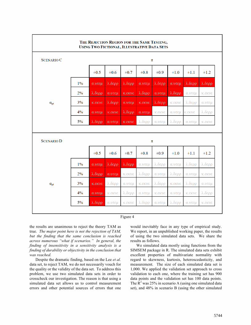
the results are unanimous to reject the theory TAM as true. The major point here is not the rejection of TAM, but the finding that the same conclusion is reached across numerous “what if scenarios.” In general, the finding of insensitivity in a sensitivity analysis is a finding of durability or objectivity in the conclusion that was reached.

Despite the dramatic finding, based on the Lee et al. data set, to reject TAM, we do not necessarily vouch for the quality or the validity of the data set. To address this problem, we use two simulated data sets in order to crosscheck our investigation. The reason is that using a simulated data set allows us to control measurement errors and other potential sources of errors that one

would inevitably face in any type of empirical study. We report, in an unpublished working paper, the results of using the two simulated data sets. We share the results as follows.

We simulated data mostly using functions from the SIMSEM package in R. The simulated data sets exhibit excellent properties of multivariate normality with regard to skewness, kurtosis, heteroscedasticity, and measurement. The size of each simulated data set is 1,000. We applied the validation set approach to cross validation to each one, where the training set has 900 data points and the validation set has 100 data points. The R2 was 25% in scenario A (using one simulated data set), and 48% in scenario B (using the other simulated

Figure 4

5744

data set). (Note that the r-square was 35% for our original field data set.) The estimates of the coefficients ßi were all statistically significant (at p < 0.001) in scenarios A and B, as they were in our original field data set. The red-shaded rejection region for scenarios A and B (see Figure 3) are altogether comparable with the rejection region we came up with using the original data set – a finding consistent with the presence of errors in the theory, TAM, rather than the presence of problems in the data. Another point worthy of mention is that the rejection region counterintuitively expands even though the R2 increases when moving from scenario A to the original field data and eventually to scenario B – a finding potentially consistent with the idea that our research method does not produce a replication of R2, which is an in-sample measure; rather, it is concerned with how well a theory performs when dealing with out-of-sample data points.

Finally, we offer, in Figure 4, two completely fictitious scenarios, C and D. Notice how the profiles of the red-shaded rejection regions are slimmer and also much closer to the table’s “northwest” corner. What we are calling the “validity frontier” is essentially the eastern “border” of the red-shaded region. In our view, the goal of theorizing using statistical inference is not so much to “prove” that the theory being tested is true in a one-off study. To the contrary, the goal is, first, to establish what the red-shaded rejection and hence, the validity frontier are in the first place, so that ongoing investigations can improve the theory (e.g., by adding, removing, or replacing variables and relationships, and even entire equations) as would become evident in the validity frontier moving further northwest compared to its location in the previous study. Therefore, in addition to making the contribution of innovating statistical research methods for prediction testing and theory testing (not just hypothesis testing), we are also contributing a conception of theorizing where the objective is not to somehow “prove” the existence of an immutable scientific law, but rather, to craft a theory over time in an extended, multi-study research program so that, as a human-made artifact, the theory can become more and more useful in making accurate, and therefore useful, predictions. 5. Conclusion

A simple and straightforward idea motivates this research. The idea is that science requires a theory to be empirically tested and to survive the empirical testing. A theory that does not survive empirical testing, much less one that has never been empirically tested in the first place, may not be considered scientific. This idea can be obscured by the extremely detailed and

sophisticated, but nonetheless necessary and helpful, statistical procedures that have been regularly used in behavioral IS research. The remedy that this paper has advanced consists of additional statistical procedures with which to restore the empirical testing of theories back to its rightful place in the repertoire of required scientific research methods.

This paper makes three contributions. First, this paper’s differentiation of empirical testing

into three different and distinct procedures, each involving its own role for statistical significance, not only gives due recognition to the continued importance of traditional hypothesis testing (which this paper names as effect testing), but also gives names to additional statistical procedures that also need to be carried out (prediction testing and theory testing) before a researcher can claim that his or her theory, operationalized as a multivariate statistical model, is scientific. Thus, a researcher who completes what he knows as just the first of these procedures would not mistakenly believe that he has completed all work required in conducting the empirical test of a theory. Henceforth, authors of research submissions to journals and conferences, along with reviewers, editors, and conference program chairs, may evaluate a theory, operationalized as a multivariate statistical model, as scientific only if it has also additionally undergone the procedures of prediction testing and theory testing.

This paper’s second contribution is a two-dimensional table useful for allowing a researcher to examine numerous “what if” scenarios in the empirical testing of a theory that is operationalized as a multivariate statistical model. In this table, each cell is a “what if” scenario reflecting two of the researcher’s judgments: (1) the judgment for his or her choice of αpt (the maximum tolerable probability, in prediction testing, for making the decision that there exists a difference between the predicted value and the observed or measured value [apart from the “noise” of sampling-induced inaccuracy in computing the prediction] when, in actuality, there is no such difference) and (2) the judgment for her choice of π (which is the researcher’s maximum tolerable prediction error, reflecting her judgment of the point at which the prediction error begins to bear sufficient practical significance so as to indicate that the prediction fails). The results can be a large number of “what if” scenarios, where the researcher can see the extent to which a conclusion that the theory is refuted (as reflected in table cells where the p-value<αtt, where αtt=0.05) is sensitive, or insensitive, to changes she can make in these two judgments. Such insensitivity would bolster the objectivity of the finding that the theory is refuted, where a larger rejection region indicates greater insensitivity.

5745

This paper’s third contribution is the concept of a theory’s validity frontier, and the associated idea that a theory is better regarded as a human-made artifact to be crafted and improved over time than as an immutable scientific law to be discovered and proved in one piece.

Together, the three contributions amount to a statistical method that uses not only statistical significance, but also practical significance to test theories. As discussed, this paper has demonstrated the method’s viability and utility, but the generalizability of the method can be established only through ongoing research. 6. References [1] “Selected Landmarks in the Development of Statistics,” A Dictionary of Statistics. Graham Upton and Ian Cook. Oxford University Press, 2008. Oxford Reference Online. Oxford University Press. [2] Davis, F. D., Bagozzi, R. P., and Warshaw, P. R. 1989. “User Acceptance of Computer Technology: A Comparison of Two Theoretical Models,” Management Science (35:8), pp. 982-1003. [3] Venkatesh, V., Morris, M. G., Davis, G. B., and Davis, F. D. 2003. “User Acceptance of Information Technology: Toward a Unified View,” MIS Quarterly (27:3), pp. 425-478. [4] Gefen, D., Rigdon, E. E., and Straub, D. 2011. “An Update and Extension to SEM Guidelines for Administrative and Social Science Research,” MIS Quarterly (35:2), pp. iii-xiv. [5] Chin, W. W., Marcolin, B. L., and Newsted, P. R. 2003. “A Partial Least Squares Latent Variable Modeling Approach for Measuring Interaction Effects: Results from a Monte Carlo Simulation Study and an Electronic-Mail Emotion/Adoption Study,” Information Systems Research (14:2), pp. 189-217. [6] Twyman, N. W., Lowry, P. B., Burgoon, J. K., and Nunamaker, J. F. 2014. “Autonomous Scientifically

Controlled Screening Systems for Detecting Information Purposely Concealed by Individuals,” Journal of Management Information Systems (31:3), pp. 106-137. [7] Compeau, D. R., Meister. D. B., and Higgins, C. A. 2007. “From Prediction to Explanation: Reconceptualizing and Extending the Perceived Characteristics of Innovating,” Journal of the Association for Information Systems (8:8), pp. 409-439. [8] Hu, T., Kettinger, W. J., and Poston, R. S. 2015. “The Effect of Online Social Value on Satisfaction and Continued Use of Social Media,” European Journal of Information Systems (24), pp. 391-410. [9] Carter, L., and Bélanger, F. 2005. “The Utilization of E-Government Services: Citizen Trust, Innovation and Acceptance Factors,” Information Systems Journal (15), pp. 5-25. [10] Jeyaraj, A., Rottman, J. W., and Lacity, M. C. 2006. “A Review of the Predictors, Linkages, and Biases in IT Innovation Adoption Research,” Journal of Information Technology (21), pp. 1-23. [11] Li, X., Hess, T. J. and Valacich, J. S. 2008. “Why Do We Trust New Technology? A Study of Initial Trust Formation with Organizational Information Systems,” Journal of Strategic Information Systems (17:1), pp. 39-71. [12] Lee, A. S., and Hubona, G. S. 2009. “A Scientific Basis for Rigor in Information Systems Research,” MIS Quarterly (33:2), pp. 237-262. [13] James, G., Witten, D., Hastie, T., and Tibshirani, R. 2014. An Introduction to Statistical Learning: With Applications in R. New York, NY: Springer. [14] University of Wyoming. 2002. “Regression,” Physics 1210 Notes, Partial Modified Appendix A. Downloaded on 3 March 2013 from uwyo.edu/ceas/classes/meref/regression.pdf.

5746