
THREE ESSAYS ON RESOURCE ALLOCATION PROBLEMS: …
165
The Pennsylvania State University The Graduate School Department of Management Science and Information Systems THREE ESSAYS ON RESOURCE ALLOCATION PROBLEMS: INVENTORY MANAGEMENT IN ASSEMBLE-TO-ORDER SYSTEMS AND ONLINE ASSIGNMENT OF FLEXIBLE RESOURCES A Thesis in Business Administration by Yal¸cınAk¸cay c 2002Yal¸cınAk¸cay Submitted in Partial Fulfillment of the Requirements for the Degree of Doctor of Philosophy December 2002
Transcript of THREE ESSAYS ON RESOURCE ALLOCATION PROBLEMS: …
The Pennsylvania State University
The Graduate School
Department of Management Science and Information Systems
THREE ESSAYS ON RESOURCE ALLOCATION PROBLEMS:
INVENTORY MANAGEMENT IN ASSEMBLE-TO-ORDER SYSTEMS
AND ONLINE ASSIGNMENT OF FLEXIBLE RESOURCES
A Thesis in
Business Administration
by
Yalcın Akcay
c© 2002 Yalcın Akcay
Submitted in Partial Fulfillmentof the Requirements
for the Degree of
Doctor of Philosophy
December 2002

We approve the thesis of Yalcın Akcay.
Date of Signature
Susan H. XuProfessor of Management ScienceThesis AdviserChair of Committee
Anantaram BalakrishnanProfessor of Management Science
Jack C. HayyaProfessor of Management Science
Natarajan GautamAssistant Professor of Industrial Engineering
John E. TyworthProfessor of Business LogisticsHead of the Department of Management Science and Information Systems

iii
ABSTRACT
This dissertation addresses two multiple resource allocation problems in operations man-
agement: an inventory management problem in an assemble-to-order (ATO) manufacturing sys-
tem and a dynamic resource allocation problem. The first essay considers a multi-component,
multi-product (ATO) system that uses an independent base-stock policy for inventory replen-
ishment. We formulate a two-stage stochastic integer program with recourse to determine the
optimal base-stock policy and the optimal component allocation policy for the system. We show
that the component allocation problem is a general multidimensional knapsack problem (MDKP)
and is NP-hard. Therefore we propose a simple, order-based component allocation rule. Intensive
testing indicates that our rule is robust, effective, and that it significantly outperforms existing
methods. We use the sample average approximation method to determine the optimal base-stock
levels. In the second essay, we exclusively concentrate on the component allocation rule proposed
for the ATO system, and study its analytical properties and computational effectiveness. Al-
though our heuristic is primarily intended for the general MDKP, it is remarkably effective also
for the 0-1 MDKP. The heuristic uses the effective capacity, defined as the maximum number of
copies of an item that can be accepted if the entire knapsack were to be used for that item alone,
as the criteria to make item selection decisions. Instead of incrementing or decrementing the value
of each decision variable by one unit in each iteration, as other heuristics do, our heuristic adds
decision variables to the solution in batches. This unique feature of the new heuristic overcomes
the inherent computational inefficiency of other general MDKP heuristics for large-scale problems.
Finally, in the third essay of the dissertation, we study a dynamic resource allocation problem, set
up in a revenue management context. An important feature of our model is that the resources are
flexible. Each customer order can potentially be satisfied using any one of the capable resources,
and the resources differ in their level of flexibility to process different demand types. We focus on
the acceptance decisions of customer demands, and the assignment decisions of resources to ac-
cepted demands. We model the revenue maximization problem as a stochastic dynamic program,
which is computationally challenging to solve. Based on our insights gained from the analysis of
special cases of the problem, we propose several approximate solutions; rollout, threshold, news-
boy and dynamic randomization heuristics. Through an extensive simulation study, we verify
that these heuristics are indeed effective in solving the problem, and are near-optimal for many
problem instances.
iv
TABLE OF CONTENTS
LIST OF TABLES . . . . . . . . . . . . . . . . . . . . . . . . . . . . . . . . . . . . . . . . vii
LIST OF FIGURES . . . . . . . . . . . . . . . . . . . . . . . . . . . . . . . . . . . . . . . ix
Chapter 1. INTRODUCTION . . . . . . . . . . . . . . . . . . . . . . . . . . . . . . . . . 1
Chapter 2. JOINT INVENTORY REPLENISHMENT AND COMPONENT ALLOCATION
OPTIMIZATION IN AN ASSEMBLE-TO-ORDER SYSTEM . . . . . . . . . 6
2.1 Introduction . . . . . . . . . . . . . . . . . . . . . . . . . . . . . . . . . . . . . 6
2.2 Literature Review . . . . . . . . . . . . . . . . . . . . . . . . . . . . . . . . . . 11
2.2.1 Literature Review on ATO Systems . . . . . . . . . . . . . . . . . . . 11
2.2.2 Literature Review on MDKP . . . . . . . . . . . . . . . . . . . . . . . 15
2.3 Problem Definition and Formulation . . . . . . . . . . . . . . . . . . . . . . . 16
2.3.1 The System . . . . . . . . . . . . . . . . . . . . . . . . . . . . . . . . . 16
2.3.2 Stochastic Integer Programming Formulation . . . . . . . . . . . . . . 20
2.3.3 Complexity of the Component Allocation Problem . . . . . . . . . . . 23
2.4 Order-Based Component Allocation Heuristics . . . . . . . . . . . . . . . . . 24
2.5 Properties of the OBCAα Heuristic . . . . . . . . . . . . . . . . . . . . . . . 30
2.6 Budget Constrained Base-Stock Optimization . . . . . . . . . . . . . . . . . . 34
2.7 Computational Results . . . . . . . . . . . . . . . . . . . . . . . . . . . . . . . 38
2.7.1 Test Problems from ATO Literature . . . . . . . . . . . . . . . . . . . 40
2.7.2 Randomly Generated Test Problems . . . . . . . . . . . . . . . . . . . 44
v
2.8 Conclusions and Future Research . . . . . . . . . . . . . . . . . . . . . . . . . 51
Chapter 3. FURTHER INVESTIGATION OF THE HEURISTIC ALGORITHM FOR THE
MULTIDIMENSIONAL KNAPSACK PROBLEM . . . . . . . . . . . . . . . 53
3.1 Introduction . . . . . . . . . . . . . . . . . . . . . . . . . . . . . . . . . . . . . 53
3.2 Algorithms for the MDKP . . . . . . . . . . . . . . . . . . . . . . . . . . . . . 56
3.2.1 The Primal Effective Capacity Heuristic (PECH) for the General MDKP 56
3.2.2 The Primal Effective Capacity Heuristic for the 0-1 MDKP . . . . . . 57
3.3 Computational Complexity . . . . . . . . . . . . . . . . . . . . . . . . . . . . 58
3.4 Computational Results . . . . . . . . . . . . . . . . . . . . . . . . . . . . . . . 63
3.4.1 Computational Results for the General MDKP . . . . . . . . . . . . . 63
3.4.1.1 Randomly Generated Test Problems . . . . . . . . . . . . . . 63
3.4.2 Computational Results for the 0-1 MDKP . . . . . . . . . . . . . . . . 69
3.4.2.1 Randomly Generated Test Problems . . . . . . . . . . . . . . 70
3.4.2.2 Benchmark Problems from the Literature . . . . . . . . . . . 75
3.4.2.3 Combinatorial Auction Problems . . . . . . . . . . . . . . . . 77
3.5 Conclusion . . . . . . . . . . . . . . . . . . . . . . . . . . . . . . . . . . . . . . 80
Chapter 4. ONLINE ASSIGNMENT OF FLEXIBLE RESOURCES . . . . . . . . . . . . 81
4.1 Introduction . . . . . . . . . . . . . . . . . . . . . . . . . . . . . . . . . . . . . 81
4.2 Review of Revenue Management Literature . . . . . . . . . . . . . . . . . . . 86
4.3 Problem Definition and Formulation . . . . . . . . . . . . . . . . . . . . . . . 88
4.3.1 Problem Definition . . . . . . . . . . . . . . . . . . . . . . . . . . . . . 88
4.3.2 Notation . . . . . . . . . . . . . . . . . . . . . . . . . . . . . . . . . . . 92
4.3.3 Problem Formulation . . . . . . . . . . . . . . . . . . . . . . . . . . . . 93

vi
4.4 Special Cases and Properties . . . . . . . . . . . . . . . . . . . . . . . . . . . 96
4.4.1 A Model for Two Types of Jobs and Three Types of Resources with
Multinomially Distributed Demand . . . . . . . . . . . . . . . . . . . . 97
4.4.2 A Model for Two Types of Jobs and Three Types of Resources with
Known Total Demand . . . . . . . . . . . . . . . . . . . . . . . . . . . 105
4.4.3 A Two Period Model for Two Types of Jobs and Three Types of Resources 110
4.4.4 Network Flow Models . . . . . . . . . . . . . . . . . . . . . . . . . . . 112
4.5 Solution Methodology . . . . . . . . . . . . . . . . . . . . . . . . . . . . . . . 116
4.5.1 Rollout Heuristic . . . . . . . . . . . . . . . . . . . . . . . . . . . . . . 117
4.5.2 Threshold Heuristic . . . . . . . . . . . . . . . . . . . . . . . . . . . . 118
4.5.3 Newsboy Heuristic . . . . . . . . . . . . . . . . . . . . . . . . . . . . . 121
4.5.4 Dynamic Randomization Heuristic . . . . . . . . . . . . . . . . . . . . 123
4.5.5 First-Come First-Served Policy . . . . . . . . . . . . . . . . . . . . . . 124
4.6 Computational Results . . . . . . . . . . . . . . . . . . . . . . . . . . . . . . . 124
4.7 Conclusions and Future Research . . . . . . . . . . . . . . . . . . . . . . . . . 135
Appendix. Proof of Proposition 14 . . . . . . . . . . . . . . . . . . . . . . . . . . . . . . . 137
REFERENCES . . . . . . . . . . . . . . . . . . . . . . . . . . . . . . . . . . . . . . . . . . 147
vii
LIST OF TABLES
2.1 Computation results for Example 2 . . . . . . . . . . . . . . . . . . . . . . . . . 28
2.2 Type-II service levels of the ATO system from Agrawal and Cohen under various
allocation rules . . . . . . . . . . . . . . . . . . . . . . . . . . . . . . . . . . . . . 47
2.3 Performance statistics of the ATO system from Agrawal and Cohen under various
allocation rules . . . . . . . . . . . . . . . . . . . . . . . . . . . . . . . . . . . . . 47
2.4 Type-II service levels of the ATO system from Zhang under various component
allocation rules . . . . . . . . . . . . . . . . . . . . . . . . . . . . . . . . . . . . . 48
2.5 Performance statistics of the ATO system from Zhang under various allocation rules 48
2.6 Estimates of the optimal base stock levels of the components in the desktop PC
assembly system from Chen et al. . . . . . . . . . . . . . . . . . . . . . . . . . . . 48
2.7 Reward ratios for the desktop PC assembly system from Chen et al. under various
component allocation rules . . . . . . . . . . . . . . . . . . . . . . . . . . . . . . 49
2.8 Performance statistics of the PC assembly system from Chen et al. . . . . . . . . 49
2.9 Reward ratio for Test Problem 4 under various heuristic rules . . . . . . . . . . 49
2.10 Performance statistics for Test Problem 4 under various heuristic rules . . . . . 50
2.11 Reward ratios for Test Problem 5 under OBCA0.5 and OBCAp0.5, with positive
time windows . . . . . . . . . . . . . . . . . . . . . . . . . . . . . . . . . . . . . 50
3.1 General MDKP - Performance statistics for all test cases . . . . . . . . . . . . . 65
3.1 General MDKP - Performance statistics for all test cases - Continued . . . . . . 66
3.2 General MDKP - Performance statistics for different number of resource constraints 67
3.3 General MDKP - Performance statistics for different number of decision variables 68

viii
3.4 General MDKP - Performance statistics for different slackness ratios . . . . . . . 69
3.5 General MDKP - Best heuristic (in terms of Mean) for different number of con-
straints and variables . . . . . . . . . . . . . . . . . . . . . . . . . . . . . . . . . . 70
3.6 0-1 MDKP - Performance statistics for all test cases . . . . . . . . . . . . . . . . 72
3.6 0-1 MDKP - Performance statistics for all test cases - Continued . . . . . . . . . 73
3.6 0-1 MDKP - Performance statistics for all test cases - Continued . . . . . . . . . 74
3.7 0-1 MDKP - Performance statistics for different number of resource constraints . 75
3.8 0-1 MDKP - Performance statistics for different number of decision variables . . 76
3.9 0-1 MDKP - Performance statistics for different slackness ratios . . . . . . . . . 76
3.10 0-1 MDKP - Best heuristic (in terms of Mean) for different number of constraints
and variables . . . . . . . . . . . . . . . . . . . . . . . . . . . . . . . . . . . . . . 76
3.11 Optimal and heuristic solutions of six 0-1 MDKP from literature . . . . . . . . . 77
3.12 Computational Results for Combinatorial Auction Problems . . . . . . . . . . . . 79
4.1 Simulation results for a system with m = 3, ` = 7 using A3, T = 30 periods,
τ = 1 period, λ = (2, 3, 4) and π3 = 100. . . . . . . . . . . . . . . . . . . . . . . . 130
4.2 Simulation results for a system with m = 3, ` = 7 using A3, T = 30 periods,
λ = (2, 3, 4), π3 = 100 and r = 0.3. . . . . . . . . . . . . . . . . . . . . . . . . . . 131
4.3 Simulation results for a system with m = 3, ` = 7 using A3, T = 30 periods,
τ = 1 period, ϕ = 2.5, α = 0.8, π3 = 100 and r = 0.3. . . . . . . . . . . . . . . . . 132
4.4 Simulation results for a system with m = 4, ` = 15 using A4, T = 20 periods,
λ = (1, 2, 3, 4), π4 = 100 and r = 0.2. . . . . . . . . . . . . . . . . . . . . . . . . . 133
4.5 Simulation results for a system with m = 5, ` = 31 using A5, T = 24 periods,
λ = (1, 2, 3, 4, 5), π5 = 100 and r = 0.2. . . . . . . . . . . . . . . . . . . . . . . . 134
ix
LIST OF FIGURES
4.1 Threshold-type optimal policy: Ft(n1) a nonincreasing function of n1 . . . . . . 104
4.2 Threshold-type optimal policy: Ft(n1) a nondecreasing function of t . . . . . . . 105

1
Chapter 1
INTRODUCTION
Resource allocation problems are central to many real-world planning problems, including
load distribution, production planning, computer scheduling and portfolio selection. They also
emerge as subproblems of more complex problems. The single resource allocation problem deter-
mines the allocation of a fixed amount of a resource to various activities, so that the objective
function under consideration is optimized. On the other hand, the multiple resource version of the
problem is a generalization that allows more than one type of resource. The modelling capability
of the problem is substantially enhanced by this generalization.
In this dissertation, we address two multiple resource allocation problems in operations
management. The first problem arises in the inventory management of assemble-to-order (ATO)
manufacturing systems, where an end-product is assembled from components or subassemblies
only when a customer order is received. These systems benefit from component commonality
and short end-product assembly times, and consequently deliver better customer service levels
and lower inventory costs. The ATO strategy has caught the attention of researchers, since it
has proven as a key competitive advantage. The majority of the research in this field is directed
towards obtaining an optimal component replenishment policy for the system, so that either a
desired level of service is achieved with the minimum inventory investment, or the service level
is maximized under a given inventory budget. However, we believe that focal points of these
studies are not always on the most critical issues. First, the importance of the component al-
location decisions is usually underestimated. In an ATO system, these decisions are made after
2
customer orders are received, based on available inventory levels. The optimal allocation can be
found by solving a computationally challenging NP-hard integer program, which opens the path
for heuristic-based allocation rules. We think that the common allocation rules in the literature
oversimplify the problem and ignore some of the underlying principles of the ATO strategy, hence
eclipse the benefits of component commonality. Second, the service level is typically measured in
terms of the proportion of the periods in which the aggregate demand is fully satisfied within the
time quoted to the customers. However, this measure reflects the service level from the system
point of view, rather than the customers’ standpoint. A more appropriate measure would be the
proportion of demand that is satisfied within the quoted time window. In our first essay, we aim to
address these two shortcomings of the existing literature. We model the periodic-review inventory
problem for a multi-product, multi-component ATO system as a two-stage stochastic nonlinear
integer program that jointly optimizes the component replenishment levels and component allo-
cations. We use the total reward from the filled customer orders to measure the service level of
the system (a measure from the customers’ perspective) and maximize it within a given inventory
investment budget constraint. We solve the first stage of the problem to determine the base-stock
levels of the components, using a Monte Carlo simulation-based technique called sample average
approximation (SAA). On the other hand, we propose a new heuristic to solve the second stage
problem, which is equivalent to an NP-hard multidimensional knapsack problem (MDKP), where
the component allocation decisions are made. Our rule synchronizes the allocation decision based
on the availability of the components required to fill an order; a component is not allocated to
an order unless that order can be completely filled. Through several numerical examples, we
illustrate that this rule is not only computationally more efficient compared to other component

3
allocation rules and integer programming heuristic methods, but also more effective in solving the
problem.
In our second essay, we concentrate exclusively on the allocation rule that we intended for
the MDKP as related to our ATO system. Our main objective is to further investigate the rule’s
analytical properties and to demonstrate its computational effectiveness. We should mention that
there is an extensive amount of research on MDKP with binary decision variables (0-1 MDKP),
but literature on the general version of the problem is relatively scarce. Moreover, the heuristics
for the general MDKP are simple extensions of their 0-1 MDKP counterparts. We attempt to fill
this void by proposing our heuristic as an approximate solution tailored primarily for the general
MDKP. Our heuristic is based on the entirely new notion of effective capacity, instead of the
traditional effective gradients approach. Effective capacity is the maximum number of items of
a particular type that can be included in the multidimensional resource (knapsack), whereas the
effective gradient is a measure of the aggregate resource consumption by an item. Consequently,
our heuristic uses the effective capacity of the selected item at a geometric rate and avoids creating
bottleneck conditions for other items. Further, our heuristic need not check solution feasibility at
any stage, unlike many of the other heuristics. We undertake an extensive computational study to
show that our pseudo-polynomial time heuristic dominates existing general MDKP heuristics, in
terms of solution time and effectiveness, and stays competitive against the 0-1 MDKP heuristics.
The resource allocation problem studied in the first two essays of this dissertation is static,
since we decouple consecutive time periods using a steady state analysis, and focus on the problem
in a typical decision period. The second problem that we consider in the dissertation, on the other
hand, is about the dynamic allocation of resources over a finite planning horizon. Additionally,
the resources in this problem are flexible. A customer demand can be satisfied with multiple

4
types of resources, and the choice of the resource to be allocated to a particular demand is
determined by the decision-maker. In other words, each flexible resource has the capability to
process more than one type of customer demand. The flexibility of a resource is a measure
of the number of different customer types that it can be assigned to. Resources have fixed
capacities, and perish after the finite planning horizon. Different customer types are associated
with different revenues. We pose this problem as a revenue management problem, in which the
decision-maker repeatedly decides whether to accept an incoming customer demand or not, and
then assigns a resource if the demand is accepted. There is a trade-off between accepting the
current demand, committing a resource and collecting the immediate return, and saving the
flexible resource for a potential future customer. This second option might potentially yield a
higher revenue, but bears the risk of having an unutilized resource at the end of the finite horizon.
The decision-maker has to consider the future demand, availability of resources, relative revenues
from different demand types, among many other things, in order to intelligently allocate the fixed
set of flexible resources to the stochastic demand so that the total revenue is maximized. We
study this challenging problem in the third essay of this dissertation. We introduce the problem
in a new context, the workplace learning industry, which has thrived in today’s technology and
innovation oriented era. A significant difference of our approach to the problem is that we adopt
the most general resource structure, allowing the use of resources at all possible levels of flexibility.
In comparison, traditional applications of revenue management in airlines, hotels, and many other
service industries, use simpler structures with a single flexible resource or resources with nested
flexibilities. Since, the stochastic dynamic programming model suffers from what is known as the
curse of dimensionality (large number of states in the state space), we study special cases of the
problem to gain insights on the structure of the optimal policy. Based on our observations from

5
the analysis of these cases, we propose several dynamic resource allocation heuristics to solve
the problem. Our comprehensive computational study indicates that these heuristics provide
near-optimal solutions in many problem instances.
In Chapter 2, we present our essay on the joint optimization of inventory replenishment and
component allocation in an assemble-to-order system. Our analysis of the approximate MDKP
solution methodology is provided in Chapter 3. Finally, Chapter 4 reports our analysis of the
online assignment of flexible resources. The detailed organization of these essays is given in the
Introduction sections of each chapter.

6
Chapter 2
JOINT INVENTORY REPLENISHMENT
AND COMPONENT ALLOCATION OPTIMIZATION
IN AN ASSEMBLE-TO-ORDER SYSTEM
2.1 Introduction
In response to increasing pressure from customers for fast delivery, mass customization,
and decreasing life cycles of products, many high-tech firms have adopted the assemble-to-order
(ATO) in place of the more traditional make-to-stock (MTS) strategy. In contrast to MTS, which
keeps inventory at the end-product level, ATO keeps inventory at the component level. When a
customer order is received, the components required are pulled from inventory and the end-product
is assembled and delivered to the customer. The ATO strategy is especially beneficial to firms
with significant component replenishment lead times and negligible final assembly times. The
ATO strategy postpones the point of commitment of components to specific products, and thus,
increases the probability of meeting a customized demand in a timely manner and at low cost (Lee
& Tang 1997). Furthermore, by using common components and modules in the final assembly,
ATO is better protected against demand variability because of risk pooling. By successfully
implementing ATO, for example, the Dell Corporation has reduced inventory costs, mitigated the
effect of product obsolescence, and thrived in the competitive PC market (Agrawal & Cohen 2000).
The IBM Personal Computing Systems Group is currently in transition from its existing MTS
operation to the ATO operation (Chen, Ettl, Lin & Yao 2000).
7
The multi-component, multi-product ATO system poses challenging inventory manage-
ment problems. One such problem is to determine inventory replenishment levels without full
information on product demands. Another problem is to make component allocation decisions
based on available component inventories and the realized product demands. Because fulfilling
a customer order requires simultaneous availability of multiple units of several components, the
optimal component allocation decisions lead to an NP-hard combinatorial optimization problem.
Although such a problem can be solved analytically, it is often impractical to implement the opti-
mal policy due to the computational complexity of the solution method and the complex structure
of the policy. It is worth-noting that the optimal component replenishment policy depends on
the component allocation rule that would be applied at a later time, which could make analytical
solutions even more difficult to obtain.
In this essay, we consider a multi-product, multi-component, periodic-review ATO system
that uses the independent base-stock (order-up-to level) policy for inventory replenishment. We
assume that the replenishment lead time of each component is an integer multiple of the review
interval and can be different for different components. Product demands in each period are
integer-valued, possibly correlated, random variables, with each product assembled from multiple
units of a subset of components. The system quotes a pre-specified response time window for
each product and receives a reward if the demand for that product is filled within its response
time window, where an order is said to be filled only if all the components requested by the order
are present.
We formulate our ATO inventory management problem as a two-stage stochastic integer
program. In the first stage, we determine the optimal base-stock levels of various components for
each review period, subject to a given inventory investment budget constraint. This decision is
8
made at the beginning of the first period without knowledge of product demands in subsequent
periods. In the second stage, we observe product demands and make component allocation de-
cisions based on the inventory on-hand and the realized demands, such that we maximize the
total reward of filled orders within their respective response time windows. When the rewards of
all product types are identical, our objective function reduces to the so-called aggregated type-II
service level, also known as the fill rate. In the inventory literature, the type-I service level mea-
sures the proportion of periods in which the demand of a product (or the aggregated demand of
all products) is met, whereas the type-II service level measures the proportion of the demand of
a product (or the proportion of the aggregated demand of all products) that is satisfied. Indeed,
a major disadvantage of the type-I service level is that it disregards the batch size effect; in con-
trast, the type-II service level often provides a much better picture of service from customers’
perspective (Asxater 2000).
We shall use the use the sample average approximation (SAA) method to solve the first-
stage of our problem. The SAA method is a Monte Carlo simulation-based solution approach to
stochastic optimization problems (Verweij, Ahmed, Kleywegt, Nemhauser & Shapiro 2001). It
is particularly suitable to treating problems whose stochastic elements have a prohibitively large
set of random scenarios and, where the use of exact mathematical programming techniques (for
example, the L-shaped method) becomes ineffective, as in our case. Roughly speaking, the SAA
method approximates the expected objective function of the stochastic program with a sample
average estimation based on a number of randomly generated scenarios. Our computational
experiments shows that the SAA method is very effective in determining the optimal base-stock
levels for our system.
9
As we noted earlier, the multi-component, multi-product allocation problem is often a
large-scale integer program and is computationally demanding. Indeed, we will show that our com-
ponent allocation problem is a large-scale, general multidimensional knapsack problem (MDKP),
which is known to be NP-hard (Garey & Johnson 1979). Although there exists an extensive lit-
erature addressing the solution procedure for the 0-1 MDKP, it appears that there is no efficient
solution procedure available to solve the large-scale, general MDKP (Lin 1998). In this essay, we
shall propose a simple, yet effective, order-based component allocation (OBCA) rule that can be
implemented in a real-time ATO environment. Unlike the component-based allocation rules in
which the component allocation decisions are made independently across different components,
such as the fixed priority (Zhang 1997) and fair shares rules (Agrawal & Cohen 2000), the OBCA
rule commits a component to an order only if it leads to the fulfillment of the order within the
quoted time window; otherwise, the component is saved for other customer orders. We show
that the OBCA rule, in the simplest version, is a polynomial-time heuristic with computational
complexity O(mn2), where m is the number of components and n the number of products. To
further improve performance, we propose a pseudo-polynomial time algorithm that uses a control
parameter, termed the greedy coefficient, to fine-tune the trade-off between solution quality and
computation time. We also develop some properties for the OBCA rule and show that under
certain agreeable conditions it locates the optimal solution. Evidently, our heuristic can also be
used to treat other general MDKPs.
We test the efficiency and effectiveness of the OBCA rule using benchmark problems from
the ATO literature and also randomly generated test problems against the performance of the
fixed priority (FP) and fair shares (FS) rules. Over a wide range of product configurations and
parameter settings, we find that the OBCA rule significantly outperforms the FP and FS rules;

10
such improvement is especially pronounced for systems with a moderate inventory budgets. The
computation time of OBCA is either smaller (for small problems) or marginally higher (for large
problems) than that required for the FP and FS rules. In fact, the OBCA rule consistently
finds near-optimal solutions with negligible average percentage errors and only requires a small
fraction of the computation time required by the optimal solutions. We also test the OBCA rule
against other MDKP heuristics, including the primal gradient method of Toyoda (1975), a greedy-
like heuristic by Loulou & Michaelides (1979), and a general MDKP heuristic by Kochenberger,
McCarl & Wyman (1974). In almost every test problem, the OBCA rule finds a better solution
than any of those heuristics, with significantly reduced computational times.
Our work has several important implications for the management of ATO systems. First,
most optimization models in ATO research focus on determining optimal base-stock levels in order
to reach a given quality of service, under some simple allocation rules (e.g., FCFS in continuous
review models and the fixed priority rule in periodic review models). It is perceived that the
customer service level depends solely on the base-stock levels and that the impact of component
allocation decisions is marginal. Our findings in this essay redress this misperception: We show
that even when there are abundant on-hand inventories to meet customer orders, the attainable
service level may not be realized due to poor component allocation decisions. In other words,
ineffective allocation rules can significantly diminish the benefits of risk pooling, which is the
underlying philosophy of component commonality in the ATO strategy. Therefore, the replen-
ishment and allocation decisions should be considered jointly in order to simultaneously lower
the base-stock levels and improve service. Second, a component-based component allocation rule,
albeit simple and easy to implement, is generally ineffective unless the service level is very high.
Our computational results indicate that under tight inventory investment budgets with attainable
11
service levels below 85%, the percentage difference between the optimal reward and the reward
collected using a component-based allocation rule can be as high as 16% (see Table 2.7). For
higher service levels, this difference is less drastic, but still significant, and can reach 6% (see
Table 2.4). Indeed, the very nature of the ATO operation, where common components are shared
by many different customer orders and each order requires simultaneous availability of several
components, implies that the firm should use an order-based allocation rule that focuses on co-
ordinated allocation decisions across different components. Fortunately, our work provides an
order-based allocation rule that is both simple and effective and suitable for real-time implemen-
tation. Finally, not only does an ineffective allocation rule degrade customer service, it can also
lead to high inventory holding costs and thus has the compounded, adverse impact on the firm’s
profit. This happens if the firm only ships completely assembled orders but still charges holding
costs to the components committed to the partially filled orders.
The remainder of this essay is organized as follows. After a review of the related literature
in Section 2.2, we formulate our two-stage stochastic program in Section 2.3. We propose a
component allocation heuristic and its variants in Section 2.4, and examine their properties in
Section 2.5. We discuss the sample average approximation method to solve the budget-constrained
base-stock optimization problem in Section 2.6. Our computational results are reported in Section
2.7. Finally, we summarize our contributions and discuss the future research in Section 2.8.
2.2 Literature Review
2.2.1 Literature Review on ATO Systems
Baker, Magazine & Nuttle (1986) studied a simple single-period, two-product ATO sys-
tem, where each product required a special component and a common component shared by both
12
products. The objective was to minimize the total safety stock of the components subject to an
aggregated type-I service level requirement. They showed that the total inventory can be reduced
by using the common component, as the result of the risk pooling of component commonality.
They also examined an alternative optimization problem, where the objective was again to min-
imize the total safety stock, but subject to the constraints that each product must satisfy its
individual type-I service level requirement. Component allocation decisions were naturally intro-
duced in this problem when the stock of the common component was not enough to meet the
demand for both products. The authors derived the analytical expressions for the component
stock levels by giving priority to the product with the smaller realized demand. Gerchak, Mag-
azine & Gamble (1988) extended the above results to a more general product structure setting
and revisited the component allocation problem. Solving a two-stage stochastic program, they
derived the optimal rationing policy for the two-product model, which gave priority to the first
product with a certain probability. In order to generalize the framework, Gerchak & Henig (1989)
considered the multi-period version of the problem and showed that the optimal solution is a
myopic policy under certain conditions. Hausman, Lee & Zhang (1998) studied a periodic re-
view, multi-component ATO system with independent order-up-to policies where demand follows
a multivariate normal distribution. They formulated a nonlinear program aiming at finding the
optimal component order-up-to levels, subject to an inventory budget constraint, that maximize
an aggregate type-I service level requirement, here defined as the probability of joint demand
fulfillment within a common time window. They proposed an equal fractile heuristic as a solution
method to determine the order-up-to levels and tested its effectiveness. Schraner (1995) investi-
gated the capacitated version of the problem and suitably modified the equal fractile heuristic of
Hausman et al. (1998).
13
There are two essays reported in the literature that directly address the component al-
location policies in the ATO system and that are particularly relevant to our research. Zhang
(1997) studied a system similar to that of Hausman et al. (1998);he was interested in determining
the order-up-to level of each component that minimized the total inventory cost, subject to a
type-I service level requirement for each product. Zhang proposed the fixed priority component
allocation rule, under which all the product demands requiring a given component were assigned a
predetermined priority order, and the available inventory of the component was allocated accord-
ingly. The ranking of products for each component was determined by factors such as product
rewards or marketing policies. Agrawal & Cohen (2000) investigated the fair shares scheme as an
alternative component allocation policy. The fair shares scheme allocated the available stock of
components to product orders, independent of the availability of the other required components.
The quantity of the component allocated to a product was determined by the ratio of the realized
demand of that product to the total realized demand of all the product orders. They derived
the analytical expression for the type-I service level for each product and further determined
the optimal component stock levels that minimized the total inventory cost, subject to prod-
uct service level requirements. It is worth mentioning that both the fixed priority rule and the
fair shares scheme are component-based allocation rules in the sense that the allocation decisions
of a component depend on the product demand of that component alone and are independent
of the allocation decisions made for other components. On the one hand, the advantage of a
component-based allocation rule is its simplicity: it is easily implemented at the local level and
does not require system-wide information. On the other hand, it is perceivable that such a rule
could result in sizable “partially” filled orders and long order response times.

14
As an alternative to these periodic review systems, Song (1998) studied a continuous-time,
base-stock ATO system. She assumed a multivariate Poisson demand process in an uncapacitated
system with deterministic lead times. Since orders arrived one by one and the first-come, first-
served rule was used to fill customer orders, the component allocation problem was irrelevant.
Song expressed the order fill rate, defined as the probability of filling an order instantaneously, by
a series of convolutions of one-dimensional Poisson distributions and proposed lower and upper
bounds for the order fill rate. Song, Xu & Bin (1999) used a set of correlated M/M/1/c queues
to model the capacitated supply in a continuous-time ATO system. They proposed a matrix-
geometric solution approach and derived exact expressions for several performance measures.
Built upon this model, Xu (1999) studied the effect of demand correlation on the performance of
the ATO system. Glasserman & Wang (1998) modelled capacitated ATO systems using correlated
MD/G/1 and GD/G/1 queues. They characterized the trade-offs between delivery lead time
and inventory. Wang (1999) proposed base-stock policies to manage the inventories in these
systems at a minimum cost subject to service level requirements. Gallien & Wein (1998) developed
analogous results for a single-product, uncapacitated stochastic assembly system where component
replenishment orders are synchronized, and obtained an approximate base-stock policy. Song &
Yao (2000) investigated a problem similar to Gallien and Wein’s, but focussed on asynchronized
systems. Chen et al. (2000) studied the configure-to-order (CTO) system, which takes the ATO
concept one step further in allowing customers to select a customized set of components that go
into the product. They used a lower bound on the fill rate of each product to achieve tractability,
and solved the optimization problem by minimizing the maximum stockout probability among all
product families subject to an inventory budget. They proposed a greedy heuristic as a solution
method and tested its effectiveness on realistic problem data.
15
2.2.2 Literature Review on MDKP
The heuristic solution methods for the 0-1 MDKP (MDKP with binary decision variables)
have generated a great deal of interest in the literature. Senju & Toyoda (1968) proposed a dual
gradient method that starts with a possibly infeasible initial solution (all decision variables set to
1) and achieves feasibility by dropping the non-rewarding variables one by one, while following
an effective gradient path. Toyoda (1975) developed a primal gradient method that improves the
initial feasible solution (all decision variables set to 0) by incrementing the value of the decision
variable with the steepest effective gradient. Exploiting the basic idea behind Toyoda’s primal
gradient method, Loulou & Michaelides (1979) developed a greedy-like algorithm that expands
the initial feasible solution by including the decision variable with the maximum pseudo-utility, a
measure of the contribution rate per unit of the aggregate resource consumption of all resources
by the decision variable. Incorporating Senju and Toyoda’s dual gradient algorithm and Everett
(1963)’s Generalized Lagrange Multipliers approach, Magazine & Oguz (1984) proposed a heuristic
method that moves from the initial infeasible solution towards a feasible solution by following
a direction which reduces the aggregate weighted infeasibility among all resource constraints.
In addition, Pirkul (1987) presented an efficient algorithm that first constructs a standard 0-1
knapsack problem using the dual variables (known as the surrogate multipliers) obtained from
the linear programming relaxation of the 0-1 MDKP; he then solves this simpler problem using
a greedy algorithm based on the ordering of the return to resource consumption ratios. We refer
the reader to the survey paper by Lin (1998) and the references therein on the results for the 0-1
MDKP and other non-standard knapsack problems.
Unlike the extensive research that has been conducted for the 0-1 MDKP, solution ap-
proaches for the general MDKP are scarce. To the best of our knowledge, only two heuristics

16
have been reported in the literature that are primarily developed for the general MDKP. Kochen-
berger et al. (1974) generalized Toyoda’s primal gradient algorithm, developed for the 0-1 MDKP,
to handle the general MDKP. This method starts with the initial feasible solution and increases
one unit of the variable with the largest effective gradient, where the effective gradient of an item
is the ratio of the reward of the item to the sum of the portions of slack consumptions of the item
over all resource constraints. Pirkul & Narasimhan (1986) extended the approximate algorithm
of Pirkul for the 0-1 MDKP to solve the general MDKP. Their method fixes the variables to their
upper bounds in sequential order of their return to consumption ratios until one or more of the
constraints of the problem are violated.
2.3 Problem Definition and Formulation
2.3.1 The System
We consider a periodic review ATO system with m components, indexed by i = 1, 2, . . . , m;
and n products, indexed by j = 1, 2, ..., n. The inventory position of each component is reviewed
at the beginning of every review period t, t = 0, 1, 2, . . .. The replenishment of component i is
controlled by an independent base-stock policy, with the base-stock level for component i denoted
by Si, i = 1, . . . , m. That is, if at the beginning of period t, the inventory position (i.e., inventory
on-hand plus inventory on order minus backorders) of component i is less than Si, then order up
to Si; otherwise, do not order. The independent base-stock policy in general is not optimal in
the ATO system, but has been adopted in analysis and in practice due to its simple structure
and easy implementation. We assume that the replenishment lead time of component i, denoted
by Li, is a constant integer that can be different for different components. After replenishment
orders are received, customer orders for different products arrive. The customer order of product

17
j in period t is denoted by random variable Pjt, where (P1t, P2t, . . . , Pnt) can be correlated for the
same period but are independent and identically distributed (iid) random vectors across different
periods.
Each product is assembled from multiple units of a subset of components. Let bij be
the number of units of component i required for one unit demand of product j, i = 1, . . . , m,
j = 1, . . . , n. The system quotes a prespecified response time window, wj , for product j and
receives a unit reward, rj , if an order of product j is filled within wj periods after its arrival,
where an order of product j is said to be filled if the order is allocated bij units of component i,
i = 1, 2, . . . , m. All unfilled orders are completely backlogged.
The problem of interest is twofold. The first set of decisions, taken at the beginning
of a period and before demand realization, is to determine the optimal base-stock levels Si,
i = 1, 2, . . . , m, that maximize the long-run average reward ratio of filling customer orders within
their respective response time windows, subject to the constraint that the total inventory invest-
ment does not exceed a given budget, B. The second set of decisions, made in each period after
the demand is realized, is to determine the amount of inventory to be allocated to the unfilled de-
mands, subject to the first-come, first-served (FCFS) order fulfillment discipline. Note that under
the FCFS rule, no inventory is committed to the orders received in later periods, unless earlier
backlogs for a component are entirely satisfied. An alternative inventory allocation scheme that
would be appropriate for such an assembly system is the earliest due date first (EDDF) principle.
According to this rule, unfilled demands with earlier due dates would receive components before
demands with later due dates. However, we will show later in the essay that, although EDDF
appears to be a plausible policy, it would have an inferior performance compared to FCFS.
We summarize the notation. For i = 1, . . . , m, j = 1, 2, . . . , n and t = 0, 1, . . . , define,

18
Pjt = Random demand for product j in period t;
bij = Usage rate of component i for one unit demand of product j;
Dit = Total demand for component i in period t=n∑
j=1bijPjt;
Ait = Replenishment of component i received in period t;
Iit = Net inventory (on-hand plus on order minus backlog) of component i at the end
of period t;
Si = Base-stock level of component i;
Li = Replenishment lead time of component i;
wj = Response time window of product j;
rj = Reward rate of filling a unit demand of product j within response time window wj .
For convenience, we sort the product indices in ascending order of their response time
windows so that
w1 ≤ w2 ≤ · · · ≤ wn = w.
Next, we derive several identities that will facilitate the formulation of our model. Let
Di[s, t] and Ai[s, t] represent the total demand and total replenishment of component i, i =
1, 2, . . . , m, from period s through period t inclusive. Then
Di[s, t] =t∑
k=s
Dik and Ai[s, t] =t∑
k=s
Aik, for i = 1, . . . , m.
Based on Hadley & Whitin (1963), the net inventory of component i at the end of period t + k
under the base-stock control Si, is given by
Ii,t+k = Si −Di[t + k − Li, t + k], i = 1, . . . ,m. (2.1)
19
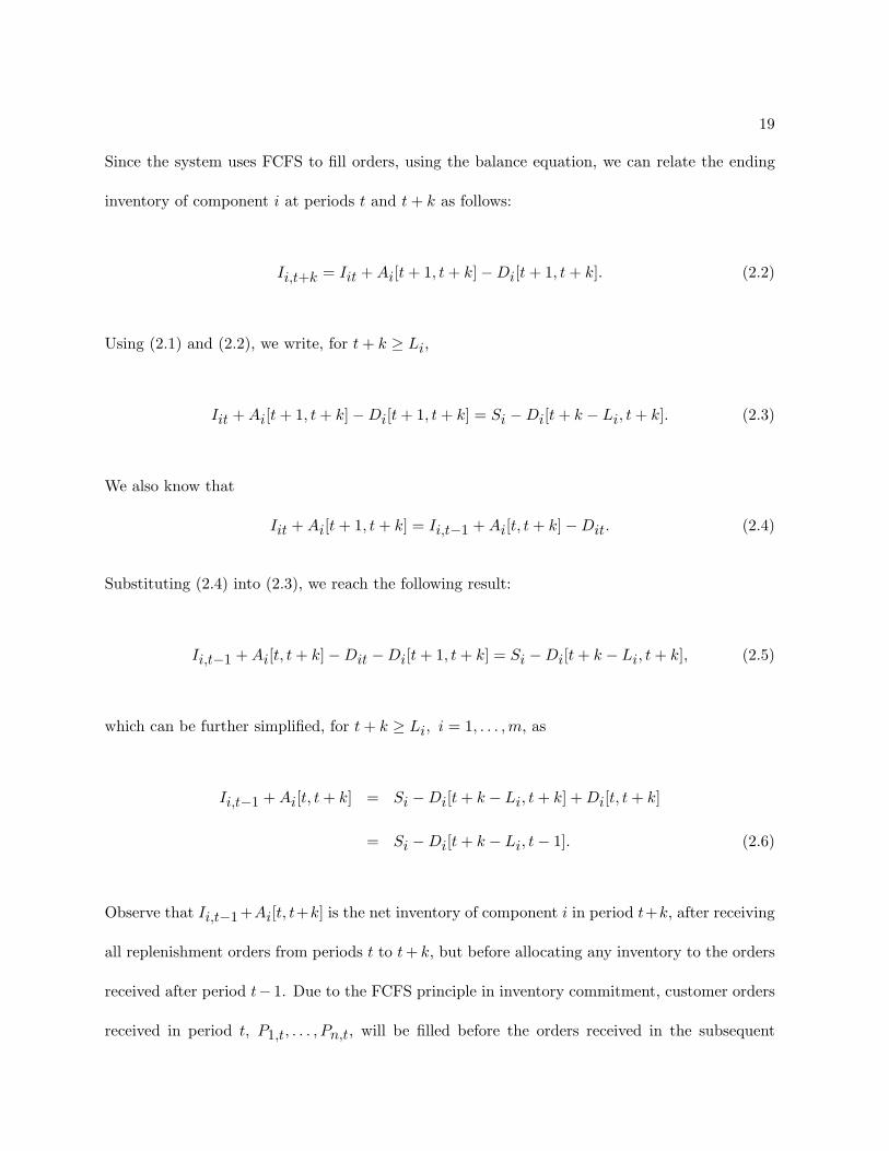
Since the system uses FCFS to fill orders, using the balance equation, we can relate the ending
inventory of component i at periods t and t + k as follows:
Ii,t+k = Iit + Ai[t + 1, t + k]−Di[t + 1, t + k]. (2.2)
Using (2.1) and (2.2), we write, for t + k ≥ Li,
Iit + Ai[t + 1, t + k]−Di[t + 1, t + k] = Si −Di[t + k − Li, t + k]. (2.3)
We also know that
Iit + Ai[t + 1, t + k] = Ii,t−1 + Ai[t, t + k]−Dit. (2.4)
Substituting (2.4) into (2.3), we reach the following result:
Ii,t−1 + Ai[t, t + k]−Dit −Di[t + 1, t + k] = Si −Di[t + k − Li, t + k], (2.5)
which can be further simplified, for t + k ≥ Li, i = 1, . . . ,m, as
Ii,t−1 + Ai[t, t + k] = Si −Di[t + k − Li, t + k] + Di[t, t + k]
= Si −Di[t + k − Li, t− 1]. (2.6)
Observe that Ii,t−1+Ai[t, t+k] is the net inventory of component i in period t+k, after receiving
all replenishment orders from periods t to t + k, but before allocating any inventory to the orders
received after period t− 1. Due to the FCFS principle in inventory commitment, customer orders
received in period t, P1,t, . . . , Pn,t, will be filled before the orders received in the subsequent
20
periods. Thus,
(Si −Di[t + k − Li, t− 1])+ = max{Si −Di[t + k − Li, t− 1], 0}
is indeed the on-hand inventory of component i available in period t + k that can be used to fill
the orders P1,t, . . . , Pn,t, provided that no inventory of component i has been allocated to those
orders since their arrival, k = 0, 1, 2, . . . , w.
In steady state, we can drop the time index t from our notation and use Di and Pj to denote
the generic versions of Dit and Pjt. We also represent the stationary version of Di[t+k−Li, t−1]
by Di(Li − k), the total stationary demand of component i in Li − k periods. In addition, we
shall assume that Li ≥ w for all i, where w = wn is the maximal response time window. This
assumption loses no generality since if Li < w for some i, then the demand for component i
from all product orders can be filled before their response time windows and component i can be
eliminated from our decisions.
2.3.2 Stochastic Integer Programming Formulation
We shall formulate our ATO inventory management problem as a two-stage stochastic inte-
ger program with recourse. In the first stage we determine the base-stock levels S = (S1, . . . , Sm)
and place our orders. Let ci be the unit purchasing cost of component i, i = 1, 2, . . . ,m. We
assume that the total inventory investment under base-stock levels S is∑m
i=1 ciSi ≤ B.
Similar to the assumption in Hausman et al. (1998), there are always Si units of component
i in the system either as on-hand or pipeline inventory and the cost of the entire inventory is
accounted for budget B. This assumption is plausible if the supplier of the components and the
assembly system are the elements of a single entity who share a common accounting scheme.

21
Further, we assume that no inventory holding cost is charged for components reserved for the
partially filled orders.
After making the base-stock level decisions, we then learn about the customer orders of
various products. Let
ξ = {(P1, . . . , Pn), Di(Li − k), i = 1, . . . ,m, k = 0, 1, ..., w}
be the collection of random demands, where P1, . . . , Pn are the product orders that arrive in the
current period (without loss of generality, designate the current period as period 0), and Di(Li−k)
is the total demand of component i generated in the previous Li − k periods, i = 1, 2, . . . , n; k =
0, 1, . . . , w. For a demand realization ξ(ω) = {(p1, . . . , pn), di(Li−k), i = 1, . . . ,m, k = 0, 1, ..., w}
and given base-stock levels S, let Qw(S, ξ(ω)) be the maximal total reward attainable from the
orders p1, p2, . . . , pn. Further, let Qw(S) be the expected value of Qw(S, ξ). The following is
then our two-stage stochastic integer programming formulation of the ATO system:
maxS
{βw(S) = 100%× Qw(S)
n∑j=1
rjE[Pj ]
}(2.7)
s.t.m∑
i=1ciSi ≤ B (2.8)
Si ≥ 0 and integer for i = 1, 2, ..., m (2.9)
where
Qw(S) = Eξ[Qw(S, ξ)], (2.10)

22
and
Qw(S, ξ(ω)) = max
{n∑
j=1
wj∑k=0
rjxjk
}(2.11)
s.t.
n∑
j=1
k∑
`=0bijxj` ≤ (Si − di(Li − k))+ for i = 1, 2, ..., m and k = 0, 1, ..., w (2.12)
w∑
k=0xjk ≤ pj for j = 1, 2, ..., n (2.13)
xjk ≥ 0 and integer for j = 1, 2, ..., n and k = 0, 1, ..., w. (2.14)
The performance measure βw(S) in (2.7) is the long-run average reward ratio, or the percentage
of total reward attainable per period, under the optimal allocation decisions for a given S. This
measure reduces to the aggregated type-II service level if all product rewards are equal. The
decision variable xjk is the number of customer orders for product j that are filled k periods after
they are received, for 0 ≤ k ≤ w. Observe from (2.11) that we do not collect rewards for the
orders filled after their response time windows. The on-hand inventory constraint for component
i in (2.12) states that the total allocation of component i within the first k periods, 0 ≤ k ≤ w,
cannot exceed the on-hand inventory of component i, (Si − di(Li − k))+, i = 1, 2, . . . ,m. The
demand constraint for product j in (2.13) ensures that the total units of product j demand filled
within its response time window do not exceed the demand of product j, pj , j = 1, 2, . . . , n.
Finally, the formulation is a nonlinear integer program, because the set of constraints given in
(2.12) are nonlinear and the decision variables are forced to take non-negative integer values by
(2.9) and (2.14).
Remember that the above two-stage stochastic program assumes an FCFS inventory com-
mitment principle. Earlier, we mentioned that an alternative to FCFS would be EDDF (earliest

23
due date first). Indeed, a very similar two-stage model to the one developed with the FCFS
assumption could be derived for the EDDF principle. With EDDF, the effective time window of
each product is reduced to zero, because no inventory will be committed to a product unless the
due date has come. In other words, the component replenishments would be accumulated during
the time window and a single allocation decision would be made when the demand is due. Note
that, this would mean a large number of unfilled orders in the system accompanied with on hand
inventories. However, in such a case, our assumption of approximating the system inventories with
the base stock levels would be violated. In order to reduce the on hand inventories, replenishment
orders might be placed so that the components would be received when the demands are due
(rather than placing the orders when the demand is received). Nevertheless, the system operating
under such a “due-date adjusted base stock policy” with zero time windows cannot meet the
performance of the FCFS system with positive time windows. In conclusion, the FCFS inventory
commitment assumption is a valid assumption which not only enables analytical tractability, but
also provides intuitive and justifiable results.
2.3.3 Complexity of the Component Allocation Problem
We now examine the computational complexity of the second-stage (recourse) program.
We consider a special case where the response time windows of all products are zero, wj = 0, j =
1, 2, . . . , n. For simplicity, let xj0 := xj , j = 0, 1, . . . , n. Then the component allocation problem
defined in (2.11)-(2.14) is to determine, for given S and ξ(ω), the immediate fills (x1, . . . , xn) that
maximize the total reward:
Q0(S, ξ(ω)) = maxn∑
j=1rjxj (2.15)
s.t.
24
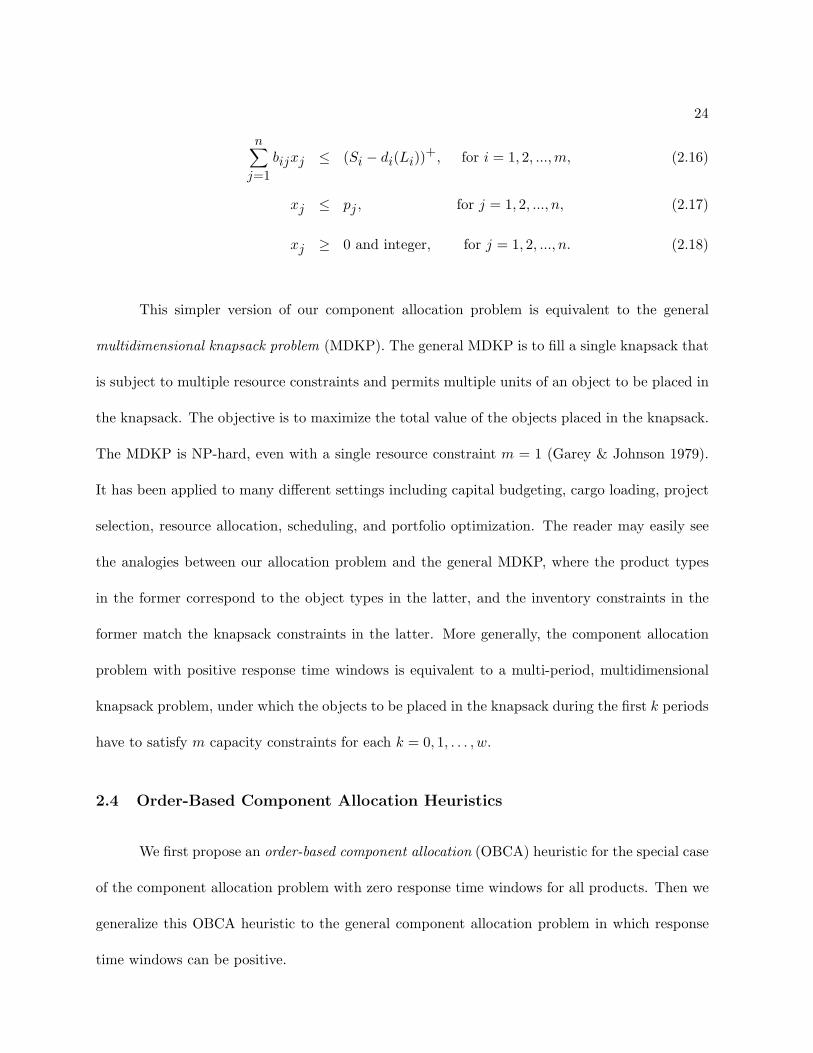
n∑
j=1bijxj ≤ (Si − di(Li))
+, for i = 1, 2, ...,m, (2.16)
xj ≤ pj , for j = 1, 2, ..., n, (2.17)
xj ≥ 0 and integer, for j = 1, 2, ..., n. (2.18)
This simpler version of our component allocation problem is equivalent to the general
multidimensional knapsack problem (MDKP). The general MDKP is to fill a single knapsack that
is subject to multiple resource constraints and permits multiple units of an object to be placed in
the knapsack. The objective is to maximize the total value of the objects placed in the knapsack.
The MDKP is NP-hard, even with a single resource constraint m = 1 (Garey & Johnson 1979).
It has been applied to many different settings including capital budgeting, cargo loading, project
selection, resource allocation, scheduling, and portfolio optimization. The reader may easily see
the analogies between our allocation problem and the general MDKP, where the product types
in the former correspond to the object types in the latter, and the inventory constraints in the
former match the knapsack constraints in the latter. More generally, the component allocation
problem with positive response time windows is equivalent to a multi-period, multidimensional
knapsack problem, under which the objects to be placed in the knapsack during the first k periods
have to satisfy m capacity constraints for each k = 0, 1, . . . , w.
2.4 Order-Based Component Allocation Heuristics
We first propose an order-based component allocation (OBCA) heuristic for the special case
of the component allocation problem with zero response time windows for all products. Then we
generalize this OBCA heuristic to the general component allocation problem in which response
time windows can be positive.
25
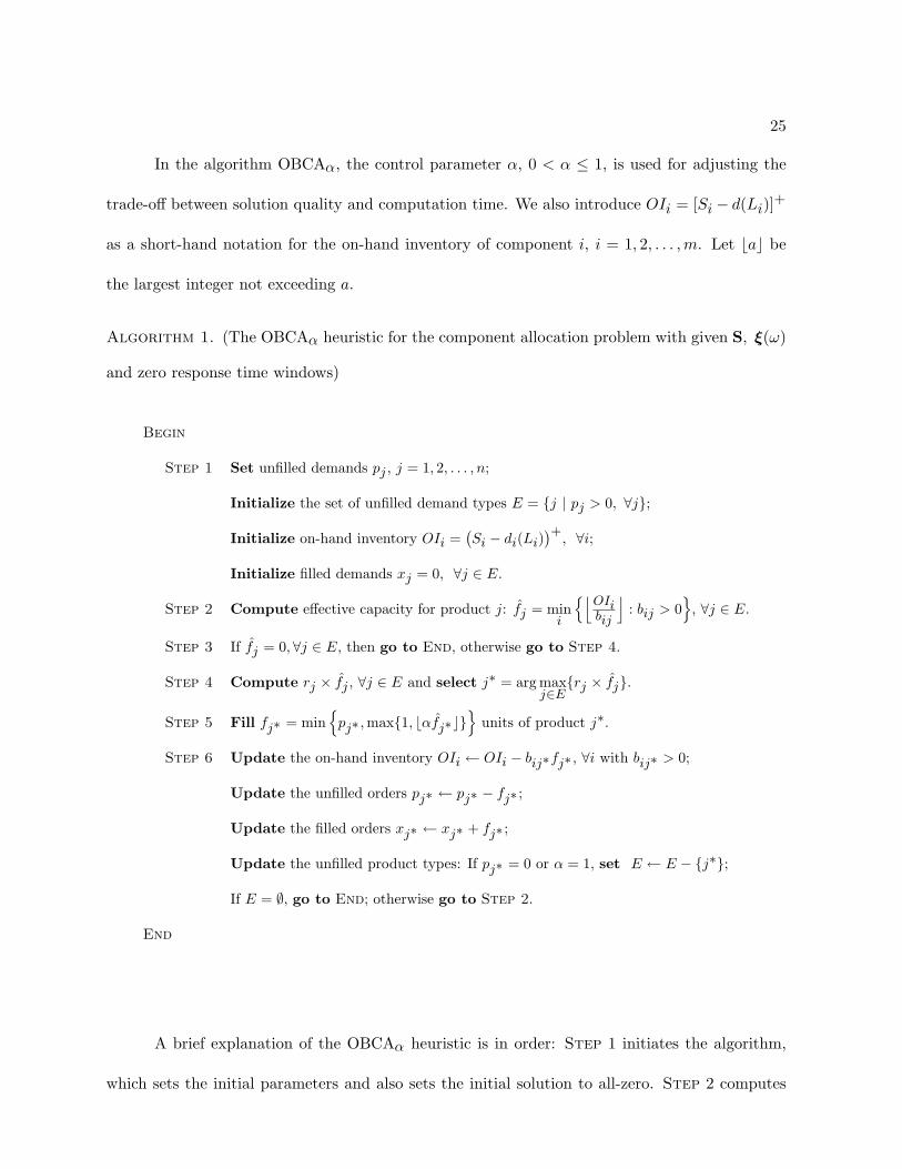
In the algorithm OBCAα, the control parameter α, 0 < α ≤ 1, is used for adjusting the
trade-off between solution quality and computation time. We also introduce OIi = [Si − d(Li)]+
as a short-hand notation for the on-hand inventory of component i, i = 1, 2, . . . , m. Let bac be
the largest integer not exceeding a.
Algorithm 1. (The OBCAα heuristic for the component allocation problem with given S, ξ(ω)
and zero response time windows)
Begin
Step 1 Set unfilled demands pj , j = 1, 2, . . . , n;
Initialize the set of unfilled demand types E = {j | pj > 0, ∀j};
Initialize on-hand inventory OIi =(Si − di(Li)
)+, ∀i;
Initialize filled demands xj = 0, ∀j ∈ E.
Step 2 Compute effective capacity for product j: fj = mini
{⌊OIibij
⌋: bij > 0
}, ∀j ∈ E.
Step 3 If fj = 0, ∀j ∈ E, then go to End, otherwise go to Step 4.
Step 4 Compute rj × fj , ∀j ∈ E and select j∗ = arg maxj∈E
{rj × fj}.
Step 5 Fill fj∗ = min{
pj∗ ,max{1, bαfj∗c}}
units of product j∗.
Step 6 Update the on-hand inventory OIi ← OIi − bij∗fj∗ , ∀i with bij∗ > 0;
Update the unfilled orders pj∗ ← pj∗ − fj∗ ;
Update the filled orders xj∗ ← xj∗ + fj∗ ;
Update the unfilled product types: If pj∗ = 0 or α = 1, set E ← E − {j∗};
If E = ∅, go to End; otherwise go to Step 2.
End
A brief explanation of the OBCAα heuristic is in order: Step 1 initiates the algorithm,
which sets the initial parameters and also sets the initial solution to all-zero. Step 2 computes
26
fj , the maximum number of product j orders that can be filled with the on-hand inventory. It
can also be regarded as the effective capacity for the product j orders, j ∈ E. Therefore, rj× fj is
understood as the maximum reward attainable if the entire effective capacity were used to fill the
product j orders. Step 4 selects product j∗ with the largest rj × fj . Step 5 fills either pj∗ units
or max{1, bαfj∗c} units of the product j∗ orders, whichever is smaller. In each iteration, the
algorithm allocates α× 100% of the effective product capacity to the selected product. Note that
the algorithm satisfies the integer conditions for the decision variables. Finally, Step 6 updates
information and returns to Step 2 for the next iteration.
The greediness of our heuristic can be adjusted by changing α, the greedy coefficient. As
α increases, the rate at which the component inventories are consumed by the selected product
in each iteration increases. For the extreme case, α = 1, the selected product can use the
maximal effective product capacity and thus will be filled to its maximal feasible units in a single
iteration. For small α, the algorithm becomes conservative in its inventory commitment to the
selected product. The algorithm might fill only a unit demand in an iteration as the system
capacity becomes tight. The use of the greedy coefficient reduces the possibility of creating
bottleneck conditions for some supply constraints, which may result in reduced rewards in future
fills. Moreover, the heuristic is likely to select different product types in consecutive iterations
since the maximal rewards may change after a few iterations. It can be seen that OBCAα is
computationally a more efficient algorithm than existing MDKP algorithms, since it depletes the
effective product capacity geometrically at rate α.
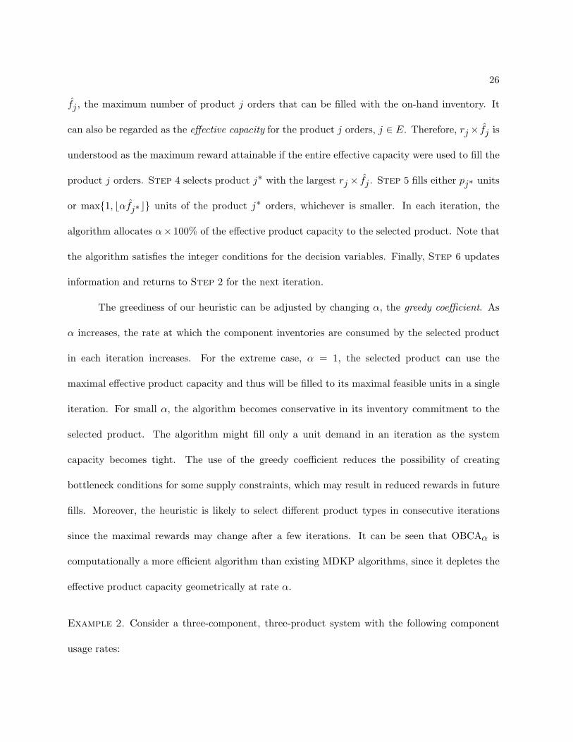
Example 2. Consider a three-component, three-product system with the following component
usage rates:
27
b =
1 1 01 2 11 0 2
Suppose we initially have OI1 = 20, OI2 = 40 and OI3 = 10 units of inventory for the
three components. Let the product demands be p1 = 20, p2 = 25 and p3 = 10. Let the product
rewards be r1 = 6, r2 = 7 and r3 = 5.
We select α = 0.5. In the first iteration, the effective capacity for each product can be
computed as
f1 = bmin{20, 40, 10}c = 10, f2 = bmin{20,402}c = 20, f3 = bmin{40,
102}c = 5,
with the maximal reward attainable for each product as
r1f1 = 6× 10 = 60, r2f2 = 7× 20 = 140, r3f3 = 5× 5 = 25.
Thus, OBCA0.5 selects product j∗ = 2 and fills min{25, b0.5 × 20c} = 10 units of product 2.
Next, we update the unfilled demand and unused on-hand inventory as p2 ← 25 − 10 = 15,
OI1 ← 20− 10 = 10, and OI2 ← 40− 2× 10 = 20, and continue with the next iteration.
The rest of the iterations to complete this example are summarized in Table 2.1. The
solution using our algorithm turns out to be x1 = 3, x2 = 17, x3 = 3, with a total reward of 152,
which is indeed the optimal solution to this problem. On the other hand, the solution under the
fair shares allocation rule is xFS1 = 5, xFS
2 = 11, xFS3 = 2, with a total reward of 117 (23% less
than optimal). Similarly, using a fixed priority rule, which allocates components first to product
2, second to product 1, and last to product 3 (a greedy priority rule based on the reward of each
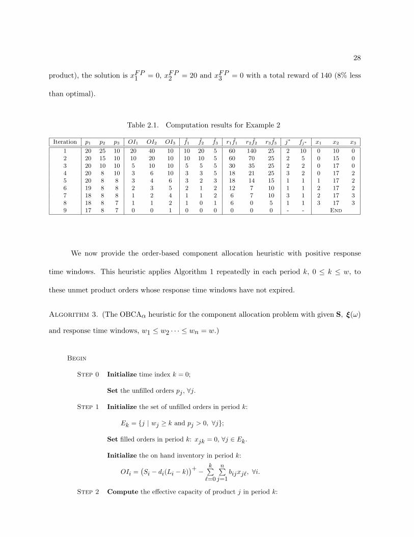
28
product), the solution is xFP1 = 0, xFP
2 = 20 and xFP3 = 0 with a total reward of 140 (8% less
than optimal).
Table 2.1. Computation results for Example 2
Iteration p1 p2 p3 OI1 OI2 OI3 f1 f2 f3 r1f1 r2f2 r3f3 j∗ fj∗ x1 x2 x3
1 20 25 10 20 40 10 10 20 5 60 140 25 2 10 0 10 02 20 15 10 10 20 10 10 10 5 60 70 25 2 5 0 15 03 20 10 10 5 10 10 5 5 5 30 35 25 2 2 0 17 04 20 8 10 3 6 10 3 3 5 18 21 25 3 2 0 17 25 20 8 8 3 4 6 3 2 3 18 14 15 1 1 1 17 26 19 8 8 2 3 5 2 1 2 12 7 10 1 1 2 17 27 18 8 8 1 2 4 1 1 2 6 7 10 3 1 2 17 38 18 8 7 1 1 2 1 0 1 6 0 5 1 1 3 17 39 17 8 7 0 0 1 0 0 0 0 0 0 - - End
We now provide the order-based component allocation heuristic with positive response
time windows. This heuristic applies Algorithm 1 repeatedly in each period k, 0 ≤ k ≤ w, to
these unmet product orders whose response time windows have not expired.
Algorithm 3. (The OBCAα heuristic for the component allocation problem with given S, ξ(ω)
and response time windows, w1 ≤ w2 · · · ≤ wn = w.)
Begin
Step 0 Initialize time index k = 0;
Set the unfilled orders pj , ∀j.
Step 1 Initialize the set of unfilled orders in period k:
Ek = {j | wj ≥ k and pj > 0, ∀j};
Set filled orders in period k: xjk = 0, ∀j ∈ Ek.
Initialize the on hand inventory in period k:
OIi =(Si − di(Li − k)
)+ −k∑
`=0
n∑j=1
bijxj`, ∀i.
Step 2 Compute the effective capacity of product j in period k:
29
fj = mini
{⌊OIibij
⌋: bij > 0
}∀j ∈ Ek.
Step 3 If fj = 0 ∀j ∈ Ek go to Step 7; otherwise go to Step 4.
Step 4 Compute rj × fj ∀j ∈ Ek and select j∗ = arg maxj∈Ek
{rj × fj}.
Break ties by selecting the product with the largest number of unfilled orders.
Step 5 Fill fj∗ = min{
pj∗ , max{1, bαfj∗c}}
units of product j∗.
Step 6 Update the on hand inventory OIi ← OIi − bij∗fj∗ , ∀i with bij∗ > 0;
Update the unfilled orders: pj∗ ← pj∗ − fj∗ ;
Update the filled orders in period k: xj∗k ← xj∗k + fj∗ ;
Update the unfilled order types: If pj∗ = 0 or α = 1, set Ek ← Ek − {j∗};
If Ek = ∅, go to Step 7; otherwise go to Step 2.
Step 7 Increment k ← k + 1. If k > w, go to End; otherwise go to Step 1.
End
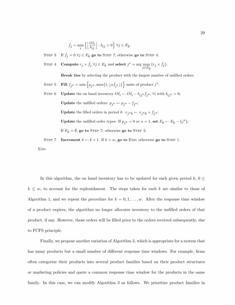
In this algorithm, the on hand inventory has to be updated for each given period k, 0 ≤
k ≤ w, to account for the replenishment. The steps taken for each k are similar to those of
Algorithm 1, and we repeat the procedure for k = 0, 1, . . . , w. After the response time window
of a product expires, the algorithm no longer allocates inventory to the unfilled orders of that
product, if any. However, those orders will be filled prior to the orders received subsequently, due
to FCFS principle.
Finally, we propose another variation of Algorithm 3, which is appropriate for a system that
has many products but a small number of different response time windows. For example, firms
often categorize their products into several product families based on their product structures
or marketing policies and quote a common response time window for the products in the same
family. In this case, we can modify Algorithm 3 as follows. We prioritize product families in

30
ascending order of their response time windows. For each period k, OBCAα starts with filling
orders of the products in the product family with the shortest response time window that has not
expired. Upon finishing the allocation for this family, it moves to fill the orders of the products
in the family with the second shortest response time window, and so on. Of course, once the
response time window of a family expires, the algorithm stops to fill the orders for the products in
that family. We will refer to this product family based component allocation rule as the OBCApα
heuristic.
2.5 Properties of the OBCAα Heuristic
We first examine the properties of OBCAα and identify the conditions under which it
locates the optimal solution. We then consider the computational complexity of OBCAα.
The next proposition states that under certain agreeable conditions, OBCAα shares the
same property as the optimal allocation policy.
Proposition 4. If rj1 ≥ rj2, wj1≤ wj2
and bi,j1 ≤ bi,j2 for i = 1, 2, ..., m, then for any
realization of demand, ξ(ω) = {p1, . . . , pn, di(Li − k), i = 1, . . . , m, k = 1, . . . , w), the following is
true:
1. Let π∗ = {x∗jk, j = 1, 2, . . . , n, k = 0, . . . , w} be the optimal solution, where x∗jk is the
number of customer orders of product j that are filled k periods after their arrival. Then,
wj1∑
k=1x∗j1,k < pj1
=⇒wj1∑
k=1x∗j2,k = 0. (2.19)

31
2. Let π = {xjk, j = 1, 2, . . . , n, k = 0, . . . , w} be the solution of the OBCAα heuristic. Then,
wj1∑
k=1xj1,k < pj1
=⇒wj1∑
k=1xj2,k = 0. (2.20)
Proof.
1. We use the interchange argument to establish (2.19). Suppose that (2.19) does not hold.
This means that under π∗ there exists a period t ≤ wj1, such that
wj1∑
k=1x∗j1,k < pj1
and x∗j2,t > 0. (2.21)
We construct another solution, π′ = {x′jk, j = 1, . . . , n, k = 0, . . . , w}, for the component
allocation problem as follows. For j = 1, 2, . . . , n and k = 0, . . . , w, let
x′jk =
x∗jk + 1, if j = j1, k = t,
x∗jk − 1, if j = j2, k = t,
x∗jk, otherwise.
(2.22)
We first show that the proposed solution π′ satisfies constraints (2.12)-(2.14) for our com-
ponent allocation problem. The integer and nonnegativity constraint (2.14) holds trivially.
The solution π′ also conforms with the demand constraint (2.13) for each product, due to
(2.21) and (2.22). Next, we check the on-hand inventory constraint (2.12) for component i,
under policy π′, for i = 1, 2, . . . , m,

32
k∑
`=0
n∑
j=1bijx
′j` =
k∑`=0
n∑j=1
bijx∗j` k = 0, 1, . . . , t− 1,
k∑`=0
n∑j=1
bijx∗j` − (bi,j2 − bi,j1) k = t, t + 1, . . . , w.
(2.23)
Because π∗ is a feasible solution and bi,j2 ≥ bi,j1 for all i, solution π′ satisfies (2.12):
k∑
`=0
n∑
j=1bijx
′j` ≤ (Si − di(Li − k))+, for k = 0, . . . , w, i = 1, 2, ..., m. (2.24)
Finally, the objective function of the allocation problem under policy π′, denoted by Q′w(S, ξ(ω)),
satisfies
Q′w(S, ξ(ω)) = Q∗w(S, ξ(ω)) + rj1 − rj2 ≥ Q∗w(S, ξ(ω)), (2.25)
since r1 ≥ r2. We thus proved, by contradiction, that (2.19) must hold.
2. The assumption bi,j1 ≤ bi,j2 implies that in each period 0 ≤ k ≤ wj1, fj1
≥ fj2in Step 2
of Algorithm 3. Consequently, rj1 fj1≥ rj2 fj2
in Step 4 of Algorithm 3, because rj1 ≥ rj2 .
Therefore, the OBCAα heuristic never fills the demand of product j2 until the demand of
product j1 is fully filled, for each 0 ≤ k ≤ wj1. 2
In the special case, rj = 1, wj = w, and bij ∈ {0, 1} for all i and j, Proposition 4 implies
that both the optimal policy and the OBCAα heuristic satisfy the small-order-first property. That
is, if product-L requests a single unit of each component in L and if L ⊆ K ⊆ {1, 2, . . . , m}, then
both policies will not fill the orders of product K unless the orders of product-L are fully satisfied.
A policy is said to be an index policy if in each period it fills customer orders according
to a predetermined sequence of product indices, as long as their response time windows have not
expired. The next result follows directly from Proposition 4.

33
Corollary 5. Suppose the following agreeable conditions are satisfied:
r1 ≥ r2 ≥ ... ≥ rn,
w1 ≤ w2 ≤ ... ≤ wn,
bi1 ≤ bi2 ≤ ... ≤ bin for i = 1, 2, ..., m.
Then,
1. The index policy {1, 2, . . . , n}, which in each period fills customer orders in the increasing
order of the product indices, starting with the product of the smallest index whose response
time window has not expired, is optimal.
2. The OBCAα heuristic becomes the index policy {1, 2, . . . , n} and hence is optimal.
Clearly, the the optimal allocation policy does not fill the demand of a product after its
response time window expires. Examining Algorithm 3, it is seen that OBCAα shares the same
property.
Now, we turn our attention to the computational complexity of the OBCAα. We shall
investigate this issue in more detail in Chapter 3. Therefore, in this section, we only summarize
our major findings.
Property 6. 1. The OBCA1 heuristic with zero time windows, given in Algorithm 1, is a
polynomial-time algorithm with the computational complexity of O(mn2).
2. The OBCAα heuristic with zero time windows, given in Algorithm 1, is a pseudo-polynomial
time algorithm with computational complexity bounded by O(mn∑n
j=1 min{pj , fj}).
3. The OBCA1 heuristic with response time windows w1 ≤ · · · ≤ wn = w, stated in Algorithm
3, is a polynomial-time algorithm with the computational complexity O(mn2w).

34
For the system with zero time windows, both algorithms of Toyoda (1975) and Loulou &
Michaelides (1979) have computational complexity of O(mn∑n
j=1 min{pj , fj}) and the algorithm
of Kochenberger et al. (1974) has the computational complexity of O(mn(∑n
j=1 min{pj , fj})2).
Therefore, OBCAα is a computationally more efficient algorithm than these, for any value of α.
Indeed, our computational tests show that OBCAα only consumes a small fraction of the CPU
time required by any other algorithm. Both the fixed priority rule of Zhang (1997) and the fair
shares scheme of Agrawal & Cohen (2000) are polynomial time algorithms with computational
complexity of O(mn). Our test results show that for small to medium-sized problems, OBCAα
often takes less CPU time, even with a small α.
2.6 Budget Constrained Base-Stock Optimization
Let us consider the budget constrained base-stock optimization problem as formulated in
Section 2.3.2. Because the number of possible scenarios for the random vector ξ in our problem
is prohibitively large, exact mathematical programming methods, such as the integer L-shaped
method of Laporte & Louveaux (1993), become inefficient. Several sampling-based approximate
solution methods to deal with such stochastic programs have been reported in the literature.
These methods rely on an estimation of Qw(S) rather than its exact value. Verweij et al. (2001)
classified these methods into two categories as interior and exterior sampling methods. Interior
sampling methods, such as the stochastic decomposition by Higle & Sen (1991), use sample
observations to estimate or construct a bound on the second-stage (the subproblem) expected
objective function. Exterior sampling methods approximate the first-stage expected objective
function (the master problem) with a sample average estimation based on a number of randomly
generated scenarios. In this essay, we use the sample average approximation (SAA) method, a
35
simple and general exterior sampling method, to solve our inventory problem. Kleywegt, Shapiro
& de Mello (2001) studied the SAA method for stochastic discrete optimization and discussed its
convergence rates and stopping rules. Verweij et al. (2001) presented a detailed computational
study of the application of the SAA method and found near-optimal solutions to three classes of
stochastic routing problems. We refer the reader to the paper by Shapiro (2000) for a survey on
variations of the SAA method.
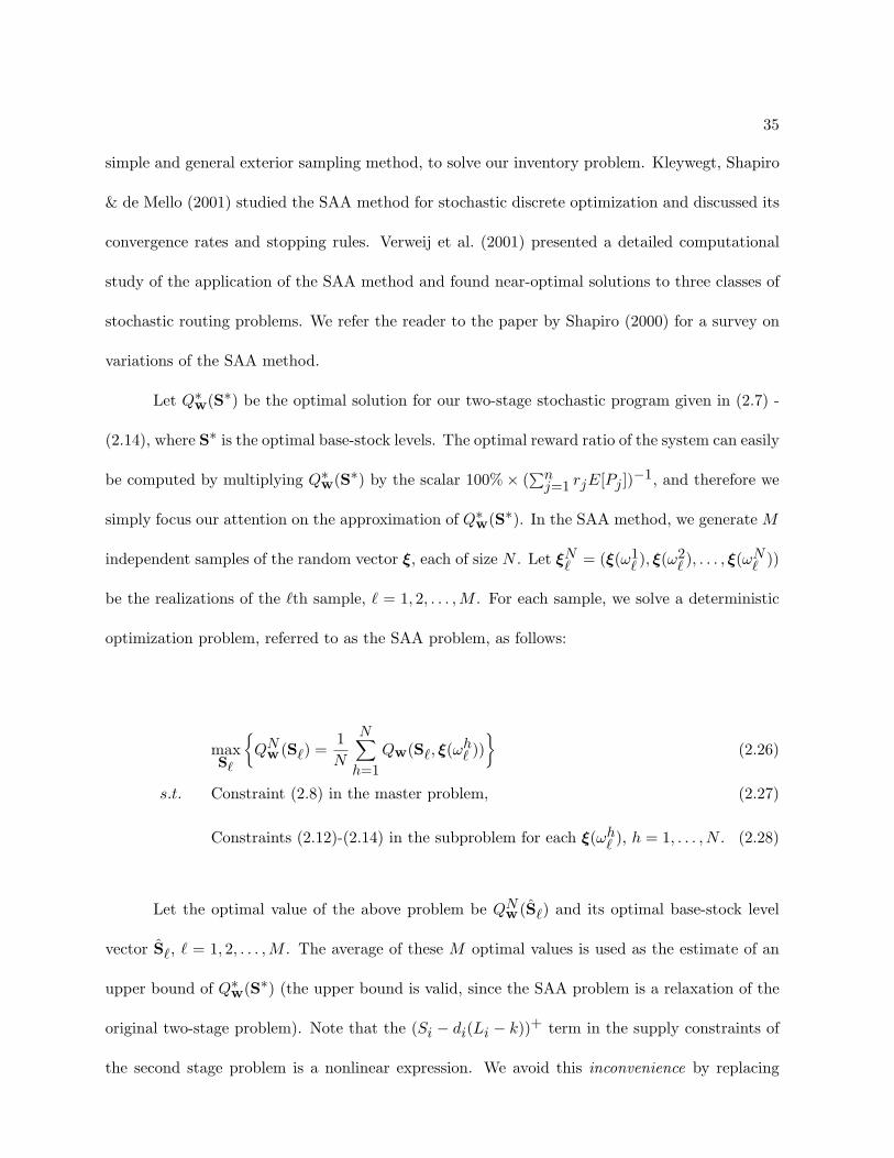
Let Q∗w(S∗) be the optimal solution for our two-stage stochastic program given in (2.7) -
(2.14), where S∗ is the optimal base-stock levels. The optimal reward ratio of the system can easily
be computed by multiplying Q∗w(S∗) by the scalar 100%× (∑n
j=1 rjE[Pj ])−1, and therefore we
simply focus our attention on the approximation of Q∗w(S∗). In the SAA method, we generate M
independent samples of the random vector ξ, each of size N . Let ξN` = (ξ(ω1
` ), ξ(ω2` ), . . . , ξ(ωN
` ))
be the realizations of the `th sample, ` = 1, 2, . . . ,M . For each sample, we solve a deterministic
optimization problem, referred to as the SAA problem, as follows:
maxS`
{QN
w (S`) =1N
N∑
h=1Qw(S`, ξ(ωh
` ))}
(2.26)
s.t. Constraint (2.8) in the master problem, (2.27)
Constraints (2.12)-(2.14) in the subproblem for each ξ(ωh` ), h = 1, . . . , N. (2.28)
Let the optimal value of the above problem be QNw (S`) and its optimal base-stock level
vector S`, ` = 1, 2, . . . ,M . The average of these M optimal values is used as the estimate of an
upper bound of Q∗w(S∗) (the upper bound is valid, since the SAA problem is a relaxation of the
original two-stage problem). Note that the (Si − di(Li − k))+ term in the supply constraints of
the second stage problem is a nonlinear expression. We avoid this inconvenience by replacing

36
the nonlinear term with Si − di(Li − k), which results in a relaxed constraint. Consequently, the
upper bound described above is still valid.
Thus,
E[QNw ] ≥ Q∗w(S∗), where QN
w =1M
M∑
`=1QN
w (S`). (2.29)
In order to achieve an unbiased estimator of Qw(S`), we generate one large independent sample,
ξN ′0 = (ξ(ω1
0), ξ(ω20), . . . , ξ(ωN ′
0 )) of size N ′ À N , and estimate the value of Qw(S`), ` =
1, 2, . . . , M , by
QN ′w (S`) =
1N ′
N ′∑
h=1Qw(S`, ξ(ωh
0 )), (2.30)
where Qw(S`, ξ(ωh0 )) is the the optimal solution of the second-stage problem with the base-stock
level vector S` and realized demand ξ(ωh0 ). Let the optimal objective function of the SAA problem
with the sample of size N ′ and the base-stock level vector S` be QN ′w (S`), ` = 1, 2, . . . , M . Out
of the M different candidate solutions, SAA chooses
S∗ ∈ argmax{QN ′
w (S`), ` = 1, . . . , M}
(2.31)
as the approximated optimal base-stock level vector. In addition, since S∗ is a feasible solution
for the original problem, E[QN ′w (S∗)] is a lower bound of Q∗w(S∗):
E[QN ′w (S∗)] ≤ Q∗w(S∗). (2.32)

37
Therefore, the difference between the upper and lower bounds can be used as an estimate
of the optimality gap. The variances of QNw and QN ′
w (S∗) are estimated as
Var(QNw ) =
1M(M − 1)
M∑
`=1(QN
w (S`)− QNw )2 (2.33)
and
Var(QN ′w (S∗)) =
1N ′(N ′ − 1)
N ′∑
h=1
[QN ′
w (S∗, ξN ′0 )− QN ′
w (S∗)]2
. (2.34)
We summarize the SAA method in the following algorithm.
Algorithm 7. (The SAA algorithm for determining the optimal base-stock levels of components)
Begin
Step 0 Select appropriate values for N , N ′ and M , and initialize ` ← 0;
Step 1 Set ` ← ` + 1 and generate an independent sample ξN` = (ξ(ω1
` ), ξ(ω2` ), . . . , ξ(ωN
` )) ;
Construct the SAA problem (2.26)-(2.28), using ξN` , and solve for S` and QN
w (S`);
If ` ≤ M go to Step 1, otherwise go to Step 2;
Step 2 Generate an independent sample ξN ′0 = (ξ(ω1
0), ξ(ω20), . . . , ξ(ωN ′
0 ));
Initialize ` ← 0;
Step 3 Set ` ← ` + 1 and construct the SAA problem using ξN ′0 and S`;
Solve for QN ′w (S`);
If ` ≤ M go to Step 3; otherwise go to Step 4;
Step 4 Choose S∗ ∈ argmax{
QN ′w (S`), ` = 1, . . . , M
};
End

38
Kleywegt et al. (2001) provide some guidelines on how to design the method by selecting
appropriate values of the sample sizes N and N ′, the number of samples M , and the stopping
criteria. As the sample size increases, the computational complexity of the SAA problem increases
at least linearly, but the solution quality of the SAA problem improves. Therefore, they suggest
that when choosing the sample size, this trade-off should be taken into consideration. Further,
if the computational effort required to solve the SAA problem increases exponentially with the
sample size, it might be beneficial to choose a smaller N but a larger M . Finally, if the optimality
gap and the variances of the estimators are too large, then the sample sizes N and N ′ should be
increased.
2.7 Computational Results
We report computational results for two sets of numerical problems. The first set of
problems is taken from the related ATO literature (Agrawal & Cohen 2000, Zhang 1997, Chen
et al. 2000), including a PC assembly system from the IBM Personal System Group. We focus on
the solutions of the budget-constrained base-stock level optimization and the optimal component
allocation decisions. We compare the OBCAα rule with the fixed priority (FS) and fair shares
(FS) rules to gain insight on the effectiveness of the OBCAα heuristic in terms its solution quality
and computation time, as the greedy coefficient α varies.
The second set of problems is obtained by using randomly generated data on reward rates,
component usage rates, lead times, and response time windows. Here, we focus on evaluating
the performance of the OBCAα rule against the optimal allocation policy and the heuristics by
Toyoda (1975), Kochenberger et al. (1974), and Loulou & Michaelides (1979).
For each problem, we shall report the following performance statistics:

39
1. The expected reward ratio βw(S) = 100% ×Eξ
[n∑
j=1
wj∑k=1
rjxjk
]
n∑j=1
rjE[Pj ], under the optimal and
heuristic allocation rules. When all product rewards are equal, the expected reward ratio
reduces to the aggregated type-II service level.
2. The percentage deviation of the average reward ratio under a given allocation rule from the
average reward ratio under the optimal allocation policy (Err.), computed as
Err. =(
1− Average reward ratio of a given allocation ruleAverage reward ratio under the optimal allocation policy
)× 100%.
3. The frequency that a given allocation rule finds the optimal solution (Hit), given by
Hit =(
Number of times the rule locates the optimal solutionNumber of simulation runs
)× 100%.
4. The percentage of the average CPU time the rule takes to obtain the solution compared
with the average CPU time to obtain the optimal solution:
CPU =(
Average CPU time the rule locates the solutionAverage CPU time to obtain the optimal solution
)× 100%.
For our computations, we coded the allocation rules and MDKP heuristics in C programming
language and used GAMS to obtain optimal solutions. We ran our tests on a 600 MHz PentiumIII
personal desktop computer.

40
2.7.1 Test Problems from ATO Literature
We study the solutions of the two-stage stochastic programs for three problems (Agrawal
& Cohen 2000, Zhang 1997, Chen et al. 2000) reported in the ATO literature. For each, the com-
ponent allocation problem is solved using Algorithm 1 or Algorithm 3. The budget-constrained
base-stock level optimization problem will be solved with the SAA method using Algorithm 7.
Based on our preliminary computations, we use M = 1000 samples, with the size of each sample
N = 50. We also set the sample size used for the unbiased estimation of the objective function
value as N ′ = 1000.
Test Problem 1. The ATO system from Agrawal & Cohen (2000). This system has
two components and four products. The component lead times and costs are L1 = 4, L2 = 6,
c1 = 10, c2 = 10. It is assumed that all the products have equal rewards and zero response time
windows. Therefore, system performance becomes the off-shelf type-II service level. Demands are
all normally distributed with parameters
P1 P2 P3 P4Mean 50 60 60 50Std. Dev. 10 15 15 10
We inflate the original demand data tenfold in order to have a wide range of demand
realizations. The coefficient of variation is 0.2 between any pair of demands. The component
usage matrix is given by
b =
[1 3 3 12 1 1 2
].
For each budget level, we find the estimate of the optimal component order-up-to levels S∗
using the SAA method. Given S∗, we then determine the type-II service levels under the optimal

41
allocation policy (OPT), the OBCAα rule with α = 0.1, 0.5, 1, the fair shares (FS) rule and the
fixed priority (FP) rule, based on 1000 simulation runs. Our findings are reported in Tables 2.2
and 2.3.
Table 2.2 shows that OBCAα significantly improves the off-shelf fill rate over the FS and
FP rules, for all selected values of α. Not surprisingly, the deviations of the fill rates from the
optimum under different rules decrease as the inventory budget increases. But even with a high
budget that achieves 90%-95% of the fill rate, OBCAα still shows a noticeable improvement over
the other two rules. Table 2.2 also shows that the solution quality of the OBCAα rule improves
as α increases, but the improvement is rather insignificant.
From Table 2.3, we observe that OBCA0.1 and OBCA0.5 find the optimal solution in each
problem instance, whereas OBCA1 achieves the optimum 73.9% of the time with an average error
of 1.57%. All the heuristics are computationally efficient and, in the worst case, they take less
than 3% of the CPU time consumed by the optimal solution. As expected, OBCAα requires more
CPU time as α decreases. For this small problem, the CPU times of OBCAα compare favorably
against those of the FS and FP rules, even with α = 0.1.
Test Problem 2. The ATO system from Zhang (1997). The ATO system consists of five
components and four products. The response time windows for all four products are equal to
1 and their rewards are also identical. The component lead times are L1 = 3, L2 = 1, L3 =
2, L4 = 4, L5 = 4 and costs are c1 = 2, c2 = 3 c3 = 6, c4 = 4 and c5 = 1. The component
usage matrix and the parameters for the normally distributed product demands are given as
b =
1 1 0 02 1 1 01 1 1 00 0 1 10 0 0 1
,

42
and
P1 P2 P3 P4Mean 100 150 50 30Std. Dev. 25 30 15 11
The type-II service level β1(S∗) reported in Table 2.4 is the percentage of demand filled
within one period of their arrival. The performance statistics of various allocation rules are
reported in Tables 2.4 and 2.5. We again observe the superiority of OBCAα over the FS and FP
rules and its near-optimal solution quality. In addition, the observations made for Test Problem
1 are also valid here.
Test Problem 3. The ATO system from Chen et al. (2000). This is a PC assembly system
with realistic problem data from the IBM Personal Systems Group. In this system, a family of
six desktop computers are to be assembled from a set of seventeen components. The demand for
each product is normally distributed with a mean of 100 and a standard deviation of 20. Other
problem parameters are given below:
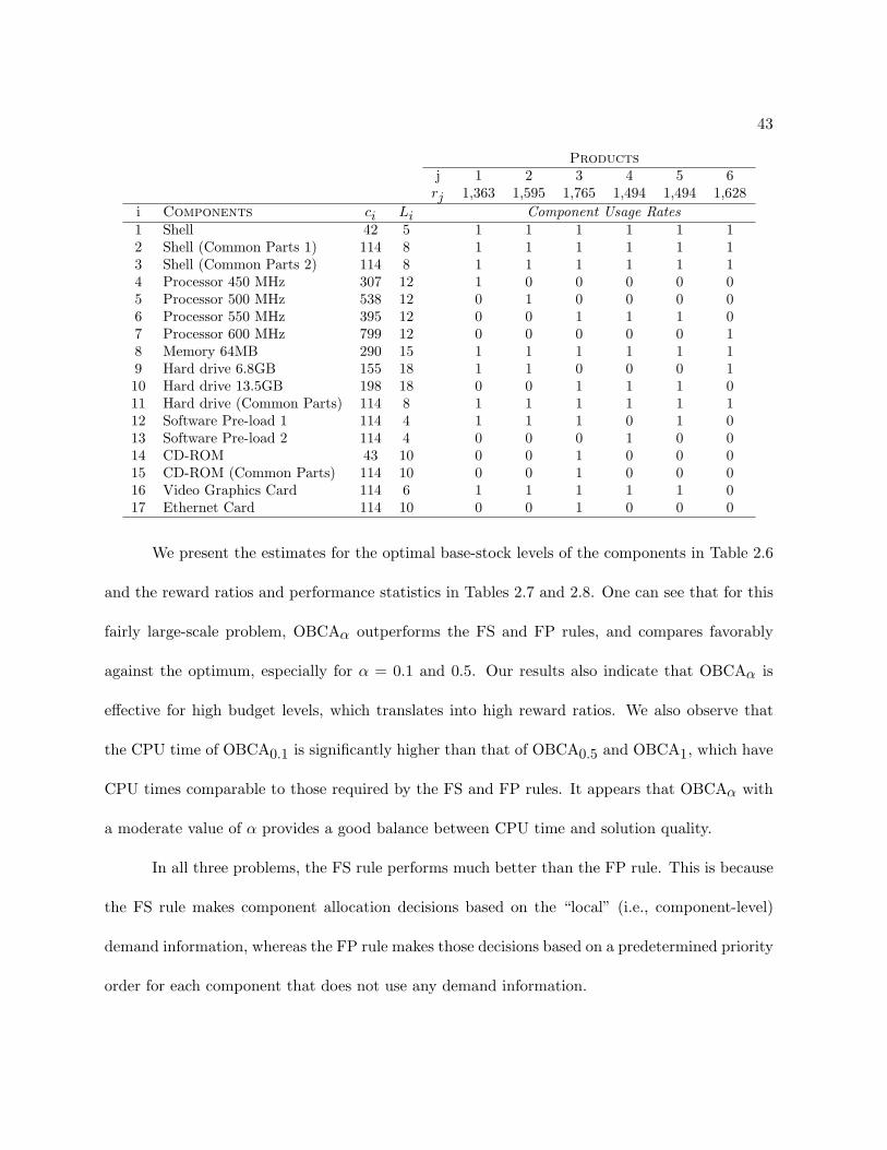
43
Productsj 1 2 3 4 5 6rj 1,363 1,595 1,765 1,494 1,494 1,628
i Components ci Li Component Usage Rates1 Shell 42 5 1 1 1 1 1 12 Shell (Common Parts 1) 114 8 1 1 1 1 1 13 Shell (Common Parts 2) 114 8 1 1 1 1 1 14 Processor 450 MHz 307 12 1 0 0 0 0 05 Processor 500 MHz 538 12 0 1 0 0 0 06 Processor 550 MHz 395 12 0 0 1 1 1 07 Processor 600 MHz 799 12 0 0 0 0 0 18 Memory 64MB 290 15 1 1 1 1 1 19 Hard drive 6.8GB 155 18 1 1 0 0 0 110 Hard drive 13.5GB 198 18 0 0 1 1 1 011 Hard drive (Common Parts) 114 8 1 1 1 1 1 112 Software Pre-load 1 114 4 1 1 1 0 1 013 Software Pre-load 2 114 4 0 0 0 1 0 014 CD-ROM 43 10 0 0 1 0 0 015 CD-ROM (Common Parts) 114 10 0 0 1 0 0 016 Video Graphics Card 114 6 1 1 1 1 1 017 Ethernet Card 114 10 0 0 1 0 0 0
We present the estimates for the optimal base-stock levels of the components in Table 2.6
and the reward ratios and performance statistics in Tables 2.7 and 2.8. One can see that for this
fairly large-scale problem, OBCAα outperforms the FS and FP rules, and compares favorably
against the optimum, especially for α = 0.1 and 0.5. Our results also indicate that OBCAα is
effective for high budget levels, which translates into high reward ratios. We also observe that
the CPU time of OBCA0.1 is significantly higher than that of OBCA0.5 and OBCA1, which have
CPU times comparable to those required by the FS and FP rules. It appears that OBCAα with
a moderate value of α provides a good balance between CPU time and solution quality.
In all three problems, the FS rule performs much better than the FP rule. This is because
the FS rule makes component allocation decisions based on the “local” (i.e., component-level)
demand information, whereas the FP rule makes those decisions based on a predetermined priority
order for each component that does not use any demand information.
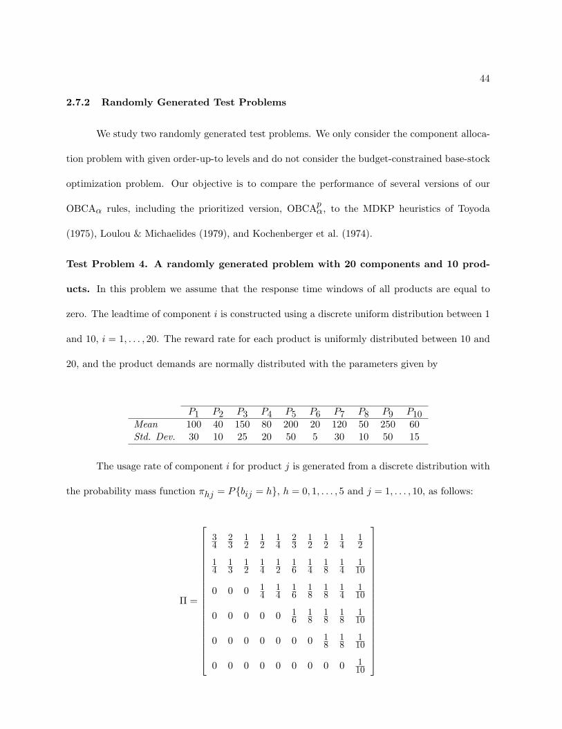
44
2.7.2 Randomly Generated Test Problems
We study two randomly generated test problems. We only consider the component alloca-
tion problem with given order-up-to levels and do not consider the budget-constrained base-stock
optimization problem. Our objective is to compare the performance of several versions of our
OBCAα rules, including the prioritized version, OBCApα, to the MDKP heuristics of Toyoda
(1975), Loulou & Michaelides (1979), and Kochenberger et al. (1974).
Test Problem 4. A randomly generated problem with 20 components and 10 prod-
ucts. In this problem we assume that the response time windows of all products are equal to
zero. The leadtime of component i is constructed using a discrete uniform distribution between 1
and 10, i = 1, . . . , 20. The reward rate for each product is uniformly distributed between 10 and
20, and the product demands are normally distributed with the parameters given by
P1 P2 P3 P4 P5 P6 P7 P8 P9 P10Mean 100 40 150 80 200 20 120 50 250 60Std. Dev. 30 10 25 20 50 5 30 10 50 15
The usage rate of component i for product j is generated from a discrete distribution with
the probability mass function πhj = P{bij = h}, h = 0, 1, . . . , 5 and j = 1, . . . , 10, as follows:
Π =
34
23
12
12
14
23
12
12
14
12
14
13
12
14
12
16
14
18
14
110
0 0 0 14
14
16
18
18
14
110
0 0 0 0 0 16
18
18
18
110
0 0 0 0 0 0 0 18
18
110
0 0 0 0 0 0 0 0 0 110

45
We define the size of a product as the total number of components required to assemble
one unit of the product. Notice that, with the above distribution, the size of the product with a
larger index is expected to rise. The order-up-to level of component i is set such that it covers the
mean component demand over Li + 1 periods, plus a certain level of safety stock,
Si = (Li + 1)E[Di] + z[(Li + 1)V ar(Di)]1/2,
where z is the safety factor. As the value of z increases, the system is better protected against
demand variation. We generate 100 problem instances and solve the component allocation problem
using OBCAα and the three heuristics for MDKP. Tables 2.9 and 2.10 report the performance
statistics.
The test results indicate that OBCA0.1 and OBCA0.5 provide the best solutions among
all the heuristic methods for every problem instance and that they are very close to the optimum.
The solution quality of OBCA1 is still acceptable, but not as good as that of Kochenberger et al.
and Toyoda, which provide excellent solutions. On the other hand, OBCAα takes only a small
fraction of computational effort compared to any other solution method. Indeed, as we noted
earlier, a unique feature of OBCAα is its ability to fill multiple units of demand in each iteration,
whereas all other heuristics fill only a unit demand in each iteration.
Test Problem 5. An ATO System with different response time windows. We con-
sider a system with ten components and nine products. The lead times of components are L =
{5, 4, 3, 4, 4, 5, 5, 3, 4, 3}. The product rewards are assumed to be r = {10, 8, 12, 14, 10, 16, 5, 6, 4}.
Product demands are normally distributed with the following parameters:

46
P1 P2 P3 P4 P5 P6 P7 P8 P9Mean 100 120 80 60 100 40 80 60 120Std. Dev. 25 30 20 15 25 10 20 15 30
The usage rates of the components are determined by the following matrix:
b =
0 1 1 0 0 1 2 0 31 1 2 0 0 0 1 2 10 0 1 2 1 0 0 2 11 2 0 1 2 2 1 2 01 0 0 0 1 0 1 1 00 1 1 0 0 1 0 1 21 0 0 2 0 0 0 0 02 0 2 1 1 1 1 0 20 1 0 1 2 0 3 2 11 0 0 1 0 2 1 1 3
The response time window of each product is equally likely to be either 0, 1, or 2 periods.
Products are grouped according to their response time windows, and the ones with the same
response time window are gathered in the same product family. The members of the product
families are different in different problem instances due to the stochastic nature of the problem.
The base-stock level of each component is set to meet the average component demand during its
effective lead time plus some safety stock, as we did in Test Problem 4. We generate 100 random
problem instances and obtain the reward ratio of the system under OBCAα and its prioritized
version, OBCApα, for α = 0.5. The results are summarized in Table 2.11. We observe that by
prioritizing product families, we can improve the system performance significantly.
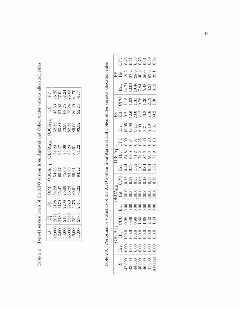
47Tab
le2.
2.T
ype-
IIse
rvic
ele
vels
ofth
eA
TO
syst
emfr
omA
graw
alan
dC
ohen
unde
rva
riou
sal
loca
tion
rule
s
BS∗ 1
S∗ 2
OP
TO
BC
A0.
1O
BC
A0.
5O
BC
A1.
0FS
FP
42,0
0020
7221
2854
.23
54.2
354
.23
52.3
845
.53
46.2
543
,000
2130
2170
65.4
765
.47
65.4
763
.81
57.0
257
.01
44,0
0021
9422
0675
.09
75.0
975
.09
73.9
568
.25
67.2
445
,000
2260
2240
83.2
383
.23
83.2
382
.38
78.2
476
.63
46,0
0023
2422
7689
.61
89.6
189
.61
89.0
686
.29
84.7
047
,000
2386
2314
94.2
294
.22
94.2
293
.92
92.2
491
.17
Tab
le2.
3.Per
form
ance
stat
isti
csof
the
AT
Osy
stem
from
Agr
awal
and
Coh
enun
der
vari
ous
allo
cati
onru
les
OB
CA
0.1
OB
CA
0.5
OB
CA
1.0
FS
FP
BE
rr.
Hit
CP
UE
rr.
Hit
CP
UE
rr.
Hit
CP
UE
rr.
Hit
CP
UE
rr.
Hit
CP
U42
,000
0.00
100.
00.
980.
0010
0.0
0.13
3.41
54.8
0.00
16.0
59.
21.
1814
.71
19.2
0.46
43,0
000.
0010
0.0
0.89
0.00
100.
00.
272.
5363
.00.
2112
.90
12.6
1.03
12.9
121
.20.
4144
,000
0.00
100.
00.
980.
0010
0.0
0.33
1.52
71.2
0.07
9.11
20.0
1.31
10.4
628
.60.
3345
,000
0.00
100.
01.
660.
0010
0.0
0.08
1.02
78.2
0.25
6.00
31.2
0.76
7.94
40.2
0.75
46,0
000.
0010
0.0
1.65
0.00
100.
00.
430.
6185
.60.
003.
7146
.81.
305.
4856
.00.
6147
,000
0.00
100.
02.
420.
0010
0.0
0.58
0.31
90.8
0.23
2.10
61.6
2.19
3.23
69.6
0.69
Ave
rage
0.00
100.
01.
430.
0010
0.0
0.30
1.57
73.9
0.13
8.31
30.2
1.30
9.12
39.1
0.54
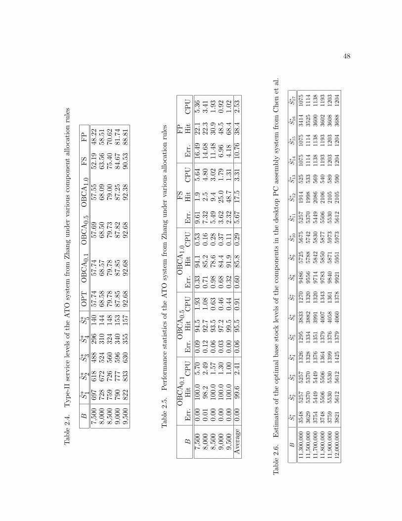
48Tab
le2.
4.T
ype-
IIse
rvic
ele
vels
ofth
eA
TO
syst
emfr
omZha
ngun
der
vari
ous
com
pone
ntal
loca
tion
rule
s
BS∗ 1
S∗ 2
S∗ 3
S∗ 4
S∗ 5
OP
TO
BC
A0.
1O
BC
A0.
5O
BC
A1.
0FS
FP
7,50
069
761
848
829
614
057
.74
57.7
457
.69
57.5
552
.19
48.2
28,
000
728
672
524
310
144
68.5
868
.57
68.5
068
.09
63.5
658
.51
8,50
075
972
656
032
414
879
.78
79.7
879
.73
79.0
075
.40
70.6
29,
000
790
777
596
340
153
87.8
587
.85
87.8
287
.25
84.6
781
.74
9,50
082
283
363
035
515
792
.68
92.6
892
.68
92.3
890
.53
88.8
1
Tab
le2.
5.Per
form
ance
stat
isti
csof
the
AT
Osy
stem
from
Zha
ngun
der
vari
ous
allo
cati
onru
les
OB
CA
0.1
OB
CA
0.5
OB
CA
1.0
FS
FP
BE
rr.
Hit
CP
UE
rr.
Hit
CP
UE
rr.
Hit
CP
UE
rr.
Hit
CP
UE
rr.
Hit
CP
U7,
500
0.00
100.
05.
700.
0994
.51.
930.
3394
.10.
539.
611.
95.
6416
.49
22.1
5.36
8,00
00.
0198
.22.
490.
1292
.71.
080.
7185
.20.
167.
322.
54.
8014
.68
22.3
3.41
8,50
00.
0010
0.0
1.57
0.06
93.5
0.63
0.98
78.6
0.28
5.49
9.4
3.02
11.4
830
.91.
939,
000
0.00
100.
01.
300.
0397
.20.
460.
6884
.40.
373.
6225
.01.
796.
9648
.50.
929,
500
0.00
100.
01.
000.
0099
.50.
440.
3291
.90.
112.
3248
.71.
314.
1868
.41.
02A
vera
ge0.
0099
.62.
410.
0695
.50.
910.
6085
.80.
295.
6717
.53.
3110
.76
38.4
2.53
Tab
le2.
6.E
stim
ates
ofth
eop
tim
alba
sest
ock
leve
lsof
the
com
pone
nts
inth
ede
skto
pP
Cas
sem
bly
syst
emfr
omC
hen
etal
.
BS∗ 1
S∗ 2
S∗ 3
S∗ 4
S∗ 5
S∗ 6
S∗ 7
S∗ 8
S∗ 9
S∗ 10
S∗ 11
S∗ 12
S∗ 13
S∗ 14
S∗ 15
S∗ 16
S∗ 17
11,3
00,0
00
3548
5257
5257
1326
1295
3833
1270
9486
5725
5675
5257
1914
525
1075
1075
3414
1075
11,5
00,0
00
3629
5370
5370
1328
1334
3882
1320
9556
5788
5742
5370
1998
533
1114
1114
3525
1114
11,7
00,0
00
3754
5449
5449
1376
1351
3991
1320
9714
5842
5830
5449
2086
569
1138
1138
3600
1138
11,8
00,0
00
3748
5506
5506
1364
1379
4007
1343
9783
5850
5877
5506
2106
540
1193
1193
3602
1193
11,9
00,0
00
3759
5530
5530
1399
1376
4058
1361
9840
5871
5973
5530
2105
589
1203
1203
3608
1203
12,0
00,0
00
3821
5612
5612
1425
1379
4060
1378
9921
5951
5973
5612
2105
590
1204
1204
3688
1204
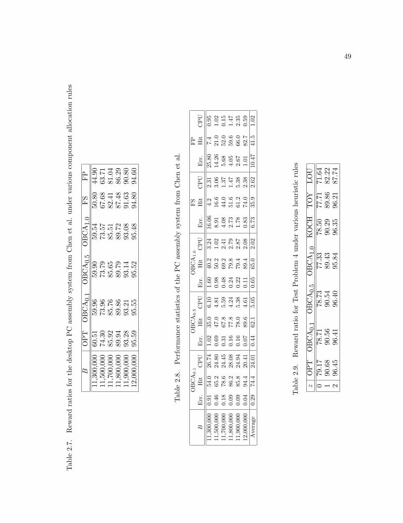
49
Tab
le2.
7.R
ewar
dra
tios
for
the
desk
top
PC
asse
mbl
ysy
stem
from
Che
net
al.
unde
rva
riou
sco
mpo
nent
allo
cati
onru
les
BO
PT
OB
CA
0.1
OB
CA
0.5
OB
CA
1.0
FS
FP
11,3
00,0
0060
.51
59.9
659
.90
59.5
450
.80
44.9
011
,500
,000
74.3
073
.96
73.7
973
.57
67.6
863
.71
11,7
00,0
0085
.92
85.7
685
.65
85.5
182
.41
81.0
411
,800
,000
89.9
489
.86
89.7
989
.72
87.4
886
.29
11,9
00,0
0093
.28
93.2
193
.14
93.0
891
.63
90.8
012
,000
,000
95.5
995
.55
95.5
295
.48
94.8
094
.60
Tab
le2.
8.Per
form
ance
stat
isti
csof
the
PC
asse
mbl
ysy
stem
from
Che
net
al.
OB
CA
0.1
OB
CA
0.5
OB
CA
1.0
FS
FP
BE
rr.
Hit
CP
UE
rr.
Hit
CP
UE
rr.
Hit
CP
UE
rr.
Hit
CP
UE
rr.
Hit
CP
U
11,3
00,0
00
0.9
154.0
26.7
41.0
235.0
6.1
01.6
040.2
3.2
416.0
64.2
2.3
125.8
07.4
0.9
511,5
00,0
00
0.4
665.2
24.8
00.6
947.0
4.8
10.9
850.2
1.0
28.9
116.6
3.0
614.2
621.0
1.0
211,7
00,0
00
0.1
878.6
24.4
50.3
167.8
5.5
90.4
869.2
2.4
14.0
844.0
1.3
75.6
852.0
0.1
511,8
00,0
00
0.0
986.2
28.0
80.1
677.8
4.2
40.2
479.8
2.7
92.7
351.6
1.4
74.0
559.6
1.4
711,9
00,0
00
0.0
985.8
24.9
40.1
678.0
5.3
80.2
279.4
2.8
71.7
861.2
5.3
82.6
766.0
2.3
512,0
00,0
00
0.0
494.4
20.4
10.0
789.6
4.6
10.1
189.4
2.0
80.8
374.0
2.3
81.0
182.7
0.5
9
Aver
age
0.2
974.4
24.0
10.4
462.1
5.0
50.6
565.0
2.0
26.7
335.9
2.6
210.4
741.5
1.0
2
Tab
le2.
9.R
ewar
dra
tio
for
Tes
tP
robl
em4
unde
rva
riou
she
uris
tic
rule
s
zO
PT
OB
CA
0.1
OB
CA
0.5
OB
CA
1.0
KO
CH
TO
YLO
U0
79.1
778
.71
78.7
377
.33
78.5
077
.71
71.6
41
90.6
890
.56
90.5
489
.43
90.2
989
.86
82.2
22
96.4
596
.41
96.4
095
.84
96.3
596
.21
87.7
4

50
Tab
le2.
10.
Per
form
ance
stat
isti
csfo
rTes
tP
robl
em4
unde
rva
riou
she
uris
tic
rule
s
OB
CA
0.1
OB
CA
0.5
OB
CA
1.0
KO
CH
TO
YLO
Uz
Err
.H
itC
PU
Err
.H
itC
PU
Err
.H
itC
PU
Err
.H
itC
PU
Err
.H
itC
PU
Err
.H
itC
PU
00.
5844
2.9
0.55
360.
62.
3229
0.2
0.84
2710
.31.
8426
16.3
9.50
840
.71
0.14
714.
160.
1666
1.0
1.39
540.
20.
4448
19.7
0.90
4530
.79.
333
78.0
20.
0383
5.9
0.05
831.
60.
6271
0.6
0.10
7436
.30.
2473
57.1
9.03
214
6.7
Avg
.0.
2566
4.3
0.25
621.
11.
4451
0.3
0.46
4922
.10.
9948
34.7
9.29
488
.5
Tab
le2.
11.
Rew
ard
rati
osfo
rTes
tP
robl
em5
unde
rO
BC
A0.
5an
dO
BC
Ap 0.
5,w
ith
posi
tive
tim
ew
indo
ws
zO
PT
OB
CA
0.5
OB
CA
p 0.5
070
.03
66.9
269
.34
174
.89
72.0
874
.69
282
.85
78.0
082
.60

51
2.8 Conclusions and Future Research
We summarize the contributions of the essay as follows.
1. We formulate a two-stage stochastic integer program to determine the optimal replenishment
policy and the optimal component allocation rule in an ATO system. Unlike most studies
reported in the literature, we adopt the the long-run average reward ratio, which reduces to
the type-II service level for identical reward rates, as the performance measure. We believe
that, for the ATO system with batch product demands, this performance measure reflects
the true meaning of service from customers’ perspective.
2. The component allocation problem in an ATO environment has not been well studied in the
literature. The two reported component allocation rules are component-based and are not
effective in the ATO environment. Here, we formulate the component allocation problem
as a general MDKP and propose the first order-based heuristic and show that it can be
solved in either polynomial or pseudo-polynomial time. Intensive testing indicates that our
heuristic is robust, efficient and effective and is suitable for real-time implementation.
3. As reported by Lin (1998), the studies toward the solution approaches to general MDKP
are scarce and most solution procedures are efficient only when the number of resource
constraints is small. To the best of our knowledge, the only approximate solution methods
for general MDKP are the effective gradient method by Kochenberger et al. (1974) and
the surrogate relaxation method by Pirkul & Narasimhan (1986). Lin also states that for
future researches, “the development of polynomial time algorithms which generate the near-
optimal solution through heuristic approaches remains attaractive”. The heuristic method
reported in this essay in most cases locates a better solution and only requires a fraction

52
of computational effort of the best available heuristic. Therefore, our heuristic can also be
used to treat the large-scale, general MDKP.
4. Our results provide several insights that enhance understanding of effective management
in the ATO systems. First, the replenishment policy and allocation decisions need to be
considered jointly in order to fully realize the benefits of risk pooling in using common
components. Second, the coordinated, order-based component allocation rule significantly
outperforms the component-based allocation rules. Finally, an ineffective allocation rule not
only degrades customer service, but it can also lead to high inventory holding costs and thus
result in a compounded, adverse impact on system performance.
Future work in this area seems promising and may take several paths. One is to consider
product-specific long-run average reward ratios, rather than using an aggregated measure for sys-
tem performance. In practice, firms often differentiate their products or product families and
prefer to attain different levels of service for each product based on their marketing policies. An-
other path we would like to consider is the relaxation of the FCFS rule in inventory commitment.
Although FCFS enhances analytical tractability, it might not be entirely valid in practice. A
more realistic model would most probably consider customer orders placed in different periods
and take into account their respective response time expiration deadlines, when making the com-
ponent allocation decision. Furthermore, we would like to extend this research to form a bridge
between periodic review and continuous review systems. A hybrid system might be developed
which would combine the benefits of the two systems.
53
Chapter 3
FURTHER INVESTIGATION OF
THE HEURISTIC ALGORITHM FOR THE
MULTIDIMENSIONAL KNAPSACK PROBLEM
3.1 Introduction
In Section 2.4 of Chapter 2, we introduced a heuristic solution method for the component
allocation problem in an assemble-to-order manufacturing system. We also demonstrated the
effectiveness of this heuristic using examples from the related ATO literature and randomly gen-
erated component allocation problems. In this essay, we explore our approximate MDKP solution
method in more detail. We further analyze the computational complexity of the algorithm, that
was briefly mentioned in the previous chapter. Moreover, we conduct an extensive computational
study of the heuristic to test its effectiveness in solving both the 0-1 (binary decision variables)
and the general versions of the MDKP, compared to other approximate solution methods. For
this purpose, we use randomly generated problems with a wide range of parameter settings, and
benchmark problems from integer programming literature.
In order for this chapter to be self-contained, we use a new set of notations that is consistent
with the one used in the MDKP literature. We consider an m-dimensional knapsack, where
the capacity of the ith dimension is bi, i = 1, 2, . . . ,m. The dimensions of the knapsack might
represent multiple resources, or different attributes of a single resource (such as weight, length and
width). There are n different items and let uj be the number of copies of item j, j = 1, 2, . . . , n.
The jth item requires aij units of the ith dimension of the knapsack, i = 1, 2, ...,m. The reward
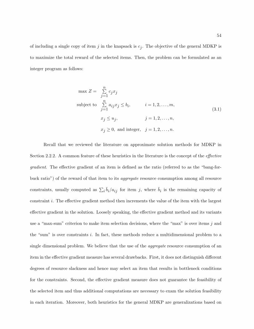
54
of including a single copy of item j in the knapsack is cj . The objective of the general MDKP is
to maximize the total reward of the selected items. Then, the problem can be formulated as an
integer program as follows:
max Z =n∑
j=1cjxj
subject ton∑
j=1aijxj ≤ bi, i = 1, 2, . . . , m,
xj ≤ uj , j = 1, 2, . . . , n,
xj ≥ 0, and integer, j = 1, 2, . . . , n.
(3.1)
Recall that we reviewed the literature on approximate solution methods for MDKP in
Section 2.2.2. A common feature of these heuristics in the literature is the concept of the effective
gradient. The effective gradient of an item is defined as the ratio (referred to as the “bang-for-
buck ratio”) of the reward of that item to its aggregate resource consumption among all resource
constraints, usually computed as∑
i bi/aij for item j, where bi is the remaining capacity of
constraint i. The effective gradient method then increments the value of the item with the largest
effective gradient in the solution. Loosely speaking, the effective gradient method and its variants
use a “max-sum” criterion to make item selection decisions, where the “max” is over items j and
the “sum” is over constraints i. In fact, these methods reduce a multidimensional problem to a
single dimensional problem. We believe that the use of the aggregate resource consumption of an
item in the effective gradient measure has several drawbacks. First, it does not distinguish different
degrees of resource slackness and hence may select an item that results in bottleneck conditions
for the constraints. Second, the effective gradient measure does not guarantee the feasibility of
the selected item and thus additional computations are necessary to exam the solution feasibility
in each iteration. Moreover, both heuristics for the general MDKP are generalizations based on

55
their respective 0-1 MDKP counterparts and, as such, they inherently increment the value of
each decision variable only by one unit in each iteration. This inevitably leads to computational
inefficiency when the decision variables can assume large values.
Remember that, our heuristic is developed on the notion of effective capacity, defined by
mini{bi/aij}, which is intuitively understood as the maximum number of copies of item j that can
be accepted if the entire remaining capacity of the knapsack were to be used for that item alone.
Our heuristic starts with the feasible solution (xj = 0 for all j) and in each iteration selects the
item that generates the highest total reward with its effective capacity, and commits a proportion,
say α, of its effective capacity to that item. As such, our heuristic always generates a feasible
solution in each iteration of the algorithm. In essence, our method uses a “max-min” criteria to
make variable selection decisions and reflects the multidimensional nature of the general MDKP.
In addition, the heuristic depletes the effective capacity at a geometric rate α and in the meantime
avoids creating bottleneck conditions for other items. The ability of our heuristic to generate a
feasible solution and to include multiple copies of the selected item in the solution in each iteration
results in superior computational efficiency over other heuristics. We refer to our heuristic as the
primal effective capacity heuristic (PECH) in the rest of the essay (this heuristic was named as
OBCA in the component allocation context). It is worth noting that although our heuristic is
primarily developed for the general MDKP, it can be tailored to treat the 0-1 MDKP. Indeed,
our computational results show that among the six competing 0-1 MDKP heuristic methods, our
heuristic ranked the best in terms of computational time and the second best in terms of solution
quality.
The rest of the essay is organized as follows. Section 3.2 proposes two versions of the primal
effective capacity heuristics, one for solving the general MDKP and another for the 0-1 MDKP,

56
and discusses computational complexity issues. Section 3.4 reports our computational results for
the general and 0-1 MDKP and compares them with the aforementioned heuristic methods in
literature. Finally, we present our conclusions in Section 3.5.
3.2 Algorithms for the MDKP
3.2.1 The Primal Effective Capacity Heuristic (PECH) for the General MDKP
In this section, we reintroduce our heuristic with the notation used in MDKP literature.
Let bac be the largest integer not exceeding a. Let α, and 0 < α ≤ 1, be a control parameter
that determines at what rate the slack of the knapsack is committed to the selected item. The
following algorithm, PECHα, describes an approximate solution procedure for the general MDKP
formulated in (3.1).
Algorithm 8. (The Algorithm of PECHα for solving the general MDKP)
Begin
Step 1 Initialize decision variables xj = 0, ∀j;
Initialize set E = {j|xj = 0, ∀j};
Initialize capacities of resources bi = bi, ∀i;
Initialize upper bounds of decision variables uj = uj , ∀j;
Step 2 Compute effective capacity for item j: yj = mini
{⌊biaij
⌋: aij > 0
}, ∀j ∈ E.
If yj = 0, ∀j ∈ E, then go to End, otherwise go to Step 3.
Step 3 Compute cj × yj , ∀j ∈ E and select j∗ = arg maxj∈E
{cj × yj}.
Step 4 Compute the increment of item j∗: yj∗ = min{
uj∗ , max{1, bαyj∗c}}
.
Step 5 Update the values of decision variables: xj∗ ← xj∗ + yj∗ ;
Update remaining capacities of constraints: bi ← bi − aij∗ × yj∗ , ∀i;
Update slacks of decision variables: uj∗ ← uj∗ − yj∗ ;
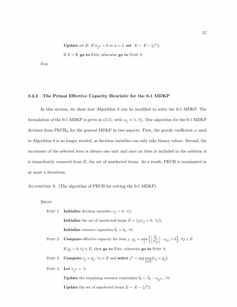
57
Update set E: If uj∗ = 0 or α = 1, set E ← E − {j∗};
If E = ∅, go to End; otherwise go to Step 2.
End
3.2.2 The Primal Effective Capacity Heuristic for the 0-1 MDKP
In this section, we show how Algorithm 8 can be modified to solve the 0-1 MDKP. The
formulation of the 0-1 MDKP is given in (3.1), with uj ≡ 1, ∀j. Our algorithm for the 0-1 MDKP
deviates from PECHα for the general MDKP in two aspects. First, the greedy coefficient α used
in Algorithm 8 is no longer needed, as decision variables can only take binary values. Second, the
increment of the selected item is always one unit and once an item is included in the solution it
is immediately removed from E, the set of unselected items. As a result, PECH is terminated in
at most n iterations.
Algorithm 9. (The algorithm of PECH for solving the 0-1 MDKP)
Begin
Step 1 Initialize decision variables xj = 0, ∀j;
Initialize the set of unselected items E = {j|xj = 0, ∀j};
Initialize resource capacities bi = bi, ∀i;
Step 2 Compute effective capacity for item j: yj = mini
{⌊biaij
⌋: aij > 0
}, ∀j ∈ E.
If yj = 0, ∀j ∈ E, then go to End, otherwise go to Step 4.
Step 3 Compute cj × yj , ∀j ∈ E and select j∗ = arg maxj∈E
{cj × yj}.
Step 4 Let xj∗ ← 1;
Update the remaining resource constraints bi ← bi − aij∗ , ∀i;
Update the set of unselected items E ← E − {j∗};

58
If E = ∅, go to End; otherwise go to Step 2.
End
3.3 Computational Complexity
In this section, we turn our attention to the computational complexity of the two algorithms
we discussed in the previous section. We show that PECHα for the general MDKP is a polynomial-
time algorithm with the computational complexity O(mn2) if α = 1 and is a pseudo polynomial-
time algorithm if 0 < α < 1. We also show that PECH for the 0-1 MDKP is a polynomial-time
algorithm with the computational complexity O(mn2).
We first consider PECHα, with α = 1, for the general MDKP described in Algorithm 8.
The effect of the initialization step, Step 1, is negligible on complexity. Steps 2 and 3 of the
algorithm require O(mn) basic operations. For α = 1, the maximum feasible number of copies of
the selected item will be included to the solution in a single iteration. Thus, the algorithm will be
repeated once for each of the n items in the worst case. This implies that PECH1 for the general
MDKP is a polynomial-time algorithm with the computational complexity O(mn2).
We next consider PECHα, with 0 < α < 1, for the general MDKP. Similar to the case
α = 1, each iteration requires O(mn) basic operations. Let kj be the number of iterations in
which item j is selected by PECHα, j = 1, 2, . . . , n, in Step 4. Clearly, kj depends on the values
of the problem parameters and the greedy coefficient α and its exact value is difficult to determine.
However, we recognize that kj ≤ min{uj ,Kj}, where Kj is the number of times that PECHα
would have selected item j if the entire knapsack capacity were to be used for the item alone and
uj = ∞, j = 1, 2, . . . , n. We shall derive an expression for Kj and use it to bound kj .

59
Let yj = mini{b biaijc} be the maximal number of copies of item j, j = 1, 2, . . . , n, that can
be packed in the knapsack, given initial capacities bi, i = 1, . . . , m. Let
R = {j : αyj < 2}.
Clearly, if j ∈ R, then PECHα will accept only one unit of item j at each iteration. We thus have
kj ≤ min{uj ,Kj} = min{uj , yj}, j ∈ R. (3.2)
Now consider j 6∈ R. Since in each iteration, the heuristic commits α × 100% of its remaining
capacity to the selected item, the number of units accepted in the kth selection of item j is
α(1−α)k−1yj (for notation simplicity we ignore the integrality constraint), if the entire effective
capacity were used for item j. Therefore, the number of iterations in which multiple copies of
item j are accepted is given by
KMj = max{k : α(1− α)k−1yj ≥ 2} =
log( 2αyj
)
log(1− α)+ 1, j 6∈ R. (3.3)
Now let KSj be the number of iterations in which PECHα accepts a single copy of item
j. It is clear that KSj must equal to the remaining effective capacity of item j after the KM
j th
selection, (1− α)KM
j yj . We thus have:
KSj = (1− α)
KMj yj ≤
2α
, j 6∈ R, (3.4)

60
where the last inequality is the result of the definition of KMj , which implies α(1−α)
KMj yj < 2,
j 6∈ R. Combining (3.3) and (3.4), we obtain, for j = 1, 2, . . . , n,
kj ≤ min{uj ,Kj} = min{uj ,KMj + KS
j }
≤ min{uj ,log( 2
αyj)
log(1− α)+
2α
+ 1}, j 6∈ R. (3.5)
From (3.2) and (3.5), we obtain the following bound for∑
j kj , the total number of iterations
under PECHα:
n∑
j=1kj = Total number of iterations of the heuristic
≤∑
j∈R
min{uj , yj}+∑
j 6∈R
min{uj ,log( 2
αyj)
log(1− α)+
2α
+ 1} (3.6)
Furthermore, if we consider the worst case when the algorithm accepts one unit of each item in
every iteration (R = {1, 2, . . . , n}), the following bound is valid from (3.2):
n∑
j=1kj ≤
n∑
j=1min{uj , yj} (3.7)
In summary, we have:
Property 10. (Computational Complexity of PECHα for the general MDKP)
1. If α = 1, then PECHα for the general MDKP, given in Algorithm 8, is a polynomial-time
algorithm with the computational complexity of O(mn2).
2. If 0 < α < 1, then PECHα for the general MDKP, given in Algorithm 8, is a pseudo
polynomial-time algorithm with its running time bounded by the computational complexity

61
of
O
(mn
∑
j 6∈R
min{uj , yj}+ mn∑
j∈R
min{uj ,log( 2
αyj)
log(1− α)+
2α
+ 1})
(3.8)
and
O
(mn
n∑
j=1min{uj , yj}
). (3.9)
Example 11. Consider the following general MDKP:
max 6x1 +7x2 +5x3subject to x1 +x2 ≤ 20
x1 +2x2 +x3 ≤ 40x1 +2x3 ≤ 10x1 ≤ 20
x2 ≤ 25x3 ≤ 10
x1, x2, x3 ≥ 0 and integer.
(3.10)
We illustrate the computation of Kj , j = 1, 2, , 3, and also verify (3.2)-(3.5). The problem
parameters are, u1 = 20, u2 = 25, u3 = 10, y1 = 10, y2 = 20, y3 = 5, and α = 0.5. Since
αyj ≥ 2 for j = 1, 2, 3, we use (3.3) and (3.4) to compute KMj and KS
j , j = 1, 2, 3, as follows:
KM1 =
log 2(0.5)(10)
log(1− 0.5)+ 1 ≈ 3, KS
1 = (1− 0.5)2(10) ≈ 3, K1 ≈ 6.
KM2 =
log 2(0.5)(20)
log(1− 0.5)+ 1 ≈ 4, KS
2 = (1− 0.5)3(20) ≈ 3, K2 ≈ 7.
and
KM3 =
log 2(0.5)(5)
log(1− 0.5)+ 1 ≈ 2, KS
3 = (1− 0.5)(5) ≈ 3, K3 ≈ 5.
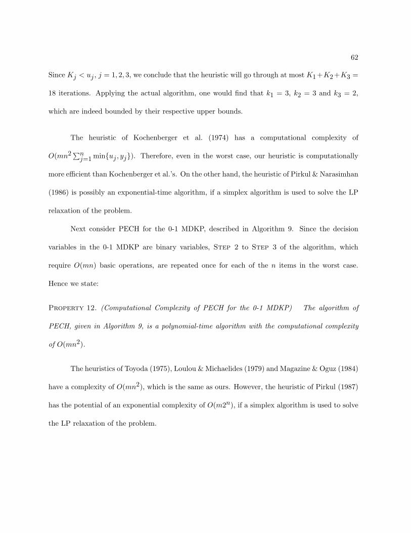
62
Since Kj < uj , j = 1, 2, 3, we conclude that the heuristic will go through at most K1+K2+K3 =
18 iterations. Applying the actual algorithm, one would find that k1 = 3, k2 = 3 and k3 = 2,
which are indeed bounded by their respective upper bounds.
The heuristic of Kochenberger et al. (1974) has a computational complexity of
O(mn2 ∑nj=1 min{uj , yj}). Therefore, even in the worst case, our heuristic is computationally
more efficient than Kochenberger et al.’s. On the other hand, the heuristic of Pirkul & Narasimhan
(1986) is possibly an exponential-time algorithm, if a simplex algorithm is used to solve the LP
relaxation of the problem.
Next consider PECH for the 0-1 MDKP, described in Algorithm 9. Since the decision
variables in the 0-1 MDKP are binary variables, Step 2 to Step 3 of the algorithm, which
require O(mn) basic operations, are repeated once for each of the n items in the worst case.
Hence we state:
Property 12. (Computational Complexity of PECH for the 0-1 MDKP) The algorithm of
PECH, given in Algorithm 9, is a polynomial-time algorithm with the computational complexity
of O(mn2).
The heuristics of Toyoda (1975), Loulou & Michaelides (1979) and Magazine & Oguz (1984)
have a complexity of O(mn2), which is the same as ours. However, the heuristic of Pirkul (1987)
has the potential of an exponential complexity of O(m2n), if a simplex algorithm is used to solve
the LP relaxation of the problem.

63
3.4 Computational Results
3.4.1 Computational Results for the General MDKP
In this section, we present our computational results of three general MDKP algorithms,
including PECHα proposed in this essay, the primal effective gradient method outlined by Kochen-
berger et al. (1974) (with legend KOCH), and the dual surrogate method proposed by Pirkul &
Narasimhan (1986) (with legend PIRG). We coded the MDKP heuristics in C programming lan-
guage and used the Cplex solver to obtain optimal solutions to the random problems. We ran
our tests on a 600 MHz PentiumIII personal desktop computer with 256MB of RAM.
In our results, we report the following performance statistics:
1. Mean: This is the mean value of the percentage error, where the percentage error of each
heuristic is measured as
percentage error = 100%× Z∗ − ZheuristicZ∗ ,
where Z∗ and Zheuristic are the optimal and heuristic solutions of the problem, respectively.
2. CPU : This is the percentage of the mean CPU time each heuristic takes to obtain the
solution compared with the average CPU time to obtain the optimal solution.
3.4.1.1 Randomly Generated Test Problems
We select the number of resource constraints, the number of decision variables, and the
slackness of the knapsack constraints as the design parameters in our numerical tests. By varying
the values of these parameters, we are able to generate a wide range of random problems. More
specifically, we generate these design parameters and other problem data as follows:

64
• The number of resource constraints m and the number of decision variables n: We choose
four levels for m, m = 10, 50, 100 and 200, and five levels for n, n = 10, 50, 100, 200 and 400;
• The greedy coefficient α: We set α = 1, 0.5 and 0.1. This allows us to observe how the
solution quality and computational time of PECHα are affected by the greediness of the
algorithm;
• We randomly generate the values of aij , cj and uj from discrete uniform distributions,
aij ∼ Unif [0, 9], cj ∼ Unif [1, 100] and uj ∼ Unif [1, 200], for all j.
• The slackness ratio Si: To generate the values of bi with various levels of resource capacities,
we adopt the slackness ratio Si introduced by Zanakis (1977):
Si = bi/n∑
j=1aijuj for i = 1, 2, . . . , m (3.11)
Note that resource capacities increase as the slackness ratio Si increases. In our compu-
tations, we first generate aij and uj as described above, and substitute them in equation
(3.11) with Si to determine bi. We use iid uniform random distributions to obtain the value
of Si for each resource constraint. We study four different cases: Si ∼ Unif(0.4, 0.6), Si ∼
Unif(0.6, 0.8), Si ∼ Unif(0.8, 0.1.0) and Si ∼ Unif(0.4, 1.0);
This setup for the computational experiments gives us 4× 5× 4 = 80 test cases. For each
test case, we generate 100 instances of aij , cj , uj and Si from their respective distributions. The
computational results for the randomly generated problems are presented in Table 3.1.
We first examine the average performance of these heuristics over 80 test cases, with 100
randomly generated instances for each case. In terms of the average of the mean errors, the
rank order of the performances of these heuristics, from the best to the worst, is PECH0.5,

65
Table 3.1. General MDKP - Performance statistics for all test cases
PECH1.0 PECH0.5 PECH0.1 KOCH PIRG
m n Si Mean CPU Mean CPU Mean CPU Mean CPU Mean CPU
10 10 (0.4-0.6) 6.62 0.04 1.50 0.09 1.58 0.17 1.62 0.04 10.54 0.04(0.6-0.8) 3.03 0.06 0.60 0.13 0.70 0.21 0.94 0.18 5.74 0.05(0.8-1.0) 1.20 0.05 0.26 0.07 0.25 0.11 0.49 0.19 2.53 0.05(0.4-1.0) 3.78 0.01 0.68 0.02 0.70 0.04 1.41 0.08 5.95 0.02
50 (0.4-0.6) 1.85 0.07 1.30 0.10 1.69 0.16 0.90 0.04 2.00 0.02(0.6-0.8) 0.64 0.03 0.41 0.08 0.52 0.13 0.44 0.21 0.82 0.07(0.8-1.0) 0.23 0.09 0.09 0.15 0.10 0.23 0.12 0.26 0.33 0.08(0.4-1.0) 0.93 0.09 0.68 0.13 0.86 0.24 0.69 0.29 0.72 0.04
100 (0.4-0.6) 1.69 0.06 1.45 0.11 1.70 0.15 0.73 0.12 1.15 0.13(0.6-0.8) 0.58 0.11 0.51 0.22 0.60 0.34 0.31 0.24 0.39 0.12(0.8-1.0) 0.13 0.06 0.08 0.12 0.10 0.19 0.07 0.24 0.14 0.15(0.4-1.0) 1.04 0.10 0.96 0.17 1.13 0.28 0.49 0.19 0.36 0.15
200 (0.4-0.6) 1.56 0.30 1.46 0.36 1.66 0.71 0.50 0.56 0.45 0.32(0.6-0.8) 0.49 0.21 0.47 0.28 0.55 0.47 0.19 0.47 0.14 0.42(0.8-1.0) 1.08 0.17 1.08 0.24 1.09 0.43 1.05 0.72 1.06 0.79(0.4-1.0) 0.94 0.24 0.96 0.30 1.04 0.61 0.36 0.67 0.10 0.52
400 (0.4-0.6) 1.53 0.64 1.50 1.18 1.65 1.87 0.42 0.93 0.22 1.18(0.6-0.8) 0.48 0.46 0.48 0.65 0.54 1.18 0.15 1.47 0.08 1.68(0.8-1.0) 0.08 0.35 0.07 0.55 0.08 0.86 0.03 2.15 0.02 2.65(0.4-1.0) 0.96 0.50 1.00 0.97 1.07 1.39 0.31 2.12 0.05 2.33
50 10 (0.4-0.6) 11.94 0.06 3.01 0.11 3.03 0.17 4.37 0.10 23.37 0.06(0.6-0.8) 7.39 0.05 1.71 0.12 1.65 0.20 2.96 0.20 15.99 0.03(0.8-1.0) 3.60 0.11 0.66 0.15 0.58 0.25 1.61 0.24 8.07 0.08(0.4-1.0) 8.39 0.03 2.07 0.05 2.50 0.08 3.45 0.14 17.94 0.05
50 (0.4-0.6) 2.94 0.16 1.92 0.19 2.08 0.38 2.25 0.12 4.95 0.11(0.6-0.8) 1.29 0.10 0.80 0.15 0.95 0.25 0.75 0.23 2.05 0.16(0.8-1.0) 0.42 0.11 0.20 0.20 0.25 0.33 0.29 0.38 0.89 0.27(0.4-1.0) 2.23 0.16 1.52 0.22 1.90 0.36 1.77 0.31 2.69 0.19
100 (0.4-0.6) 2.23 0.22 1.72 0.40 1.99 0.82 1.74 0.53 2.72 0.33(0.6-0.8) 0.89 0.17 0.64 0.24 0.78 0.49 0.79 0.79 1.07 0.51(0.8-1.0) 0.24 0.14 0.15 0.32 0.18 0.48 0.24 1.11 0.38 0.76(0.4-1.0) 1.94 0.26 1.64 0.53 1.96 0.83 1.38 0.82 1.54 0.68
200 (0.4-0.6) 1.74 1.07 1.51 1.36 1.72 2.68 1.18 1.17 1.33 1.36(0.6-0.8) 0.73 0.80 0.63 1.03 0.73 1.74 0.59 2.09 0.56 1.98(0.8-1.0) 0.17 0.50 0.14 0.68 0.16 1.24 0.16 3.27 0.16 3.32(0.4-1.0) 1.59 0.69 1.45 1.23 1.68 2.01 0.96 2.80 0.69 3.03
400 (0.4-0.6) 1.61 2.93 1.54 5.69 1.70 9.23 0.92 4.53 0.66 4.98(0.6-0.8) 0.59 1.94 0.55 3.35 0.62 5.79 0.39 6.59 0.28 8.91(0.8-1.0) 0.15 1.54 0.13 2.21 0.15 3.73 0.11 9.68 0.08 13.26(0.4-1.0) 1.61 2.57 1.58 4.51 1.75 7.48 0.91 10.52 0.26 10.44
Continued on next page

66
Table 3.1. General MDKP - Performance statistics for all test cases - Continued
Continuing from previous page
PECH1.0 PECH0.5 PECH0.1 KOCH PIRG
m n Si Mean CPU Mean CPU Mean CPU Mean CPU Mean CPU
100 10 (0.4-0.6) 13.14 0.03 2.65 0.04 2.88 0.08 5.63 0.03 31.62 0.06(0.6-0.8) 8.19 0.04 1.80 0.06 1.76 0.12 3.87 0.04 21.00 0.04(0.8-1.0) 4.34 0.06 0.80 0.11 0.63 0.21 2.25 0.18 10.88 0.04(0.4-1.0) 9.80 0.08 2.37 0.13 2.60 0.25 4.95 0.14 21.18 0.05
50 (0.4-0.6) 3.52 0.22 2.17 0.35 2.21 0.59 2.77 0.22 6.46 0.21(0.6-0.8) 1.60 0.20 0.85 0.28 0.95 0.46 1.35 0.33 3.13 0.22(0.8-1.0) 0.58 0.13 0.26 0.19 0.28 0.35 0.45 0.60 1.29 0.42(0.4-1.0) 2.78 0.18 1.74 0.26 1.95 0.45 2.16 0.54 4.16 0.36
100 (0.4-0.6) 2.34 0.69 1.73 1.01 1.96 1.44 2.07 0.83 3.72 0.74(0.6-0.8) 1.04 0.36 0.74 0.65 0.79 1.02 0.90 1.26 1.39 1.01(0.8-1.0) 1.04 0.29 0.74 0.41 0.79 0.66 0.90 1.85 1.39 1.48(0.4-1.0) 1.97 0.45 1.68 0.87 1.97 1.25 1.85 1.65 2.06 1.40
200 (0.4-0.6) 1.82 1.95 1.51 2.79 1.71 5.72 1.48 2.74 1.75 2.67(0.6-0.8) 0.76 1.13 0.60 1.87 0.67 3.14 0.64 4.07 0.68 4.35(0.8-1.0) 0.19 0.67 0.13 1.19 0.16 2.16 0.21 7.32 0.24 6.71(0.4-1.0) 1.78 1.63 1.58 2.23 1.82 4.27 1.33 4.42 1.09 4.94
400 (0.4-0.6) 1.60 6.05 1.47 10.15 1.61 17.57 1.24 8.39 0.83 9.95(0.6-0.8) 0.59 3.86 0.52 5.77 0.59 11.05 0.48 12.34 0.39 15.79(0.8-1.0) 0.15 2.94 0.13 4.46 0.15 7.65 0.15 20.74 0.13 26.46(0.4-1.0) 1.56 3.75 1.50 7.53 1.72 14.22 1.05 16.89 0.57 19.54
200 10 (0.4-0.6) 18.91 0.09 3.23 0.11 3.22 0.22 8.37 0.24 33.09 0.02(0.6-0.8) 11.74 0.03 2.25 0.07 2.21 0.12 6.43 0.22 25.72 0.06(0.8-1.0) 5.46 0.08 0.84 0.11 0.90 0.21 3.21 0.27 14.57 0.05(0.4-1.0) 13.67 0.10 2.34 0.14 2.67 0.27 6.78 0.29 27.73 0.09
50 (0.4-0.6) 3.84 0.41 2.28 0.56 2.25 0.99 3.44 0.57 8.48 0.40(0.6-0.8) 1.70 0.15 1.01 0.31 1.06 0.59 1.64 0.80 3.55 0.46(0.8-1.0) 0.73 0.13 0.31 0.24 0.32 0.43 0.63 1.25 1.34 0.78(0.4-1.0) 3.06 0.28 1.79 0.51 1.99 0.78 2.73 0.89 6.01 0.75
100 (0.4-0.6) 2.59 1.23 1.92 1.93 1.97 3.03 2.47 1.49 4.69 1.43(0.6-0.8) 1.12 0.66 0.76 0.95 0.86 1.80 1.20 2.55 1.86 2.27(0.8-1.0) 0.39 0.56 0.23 0.68 0.24 1.37 0.43 3.40 0.62 3.38(0.4-1.0) 2.27 1.10 1.76 1.58 1.96 2.50 2.23 2.99 3.01 2.62
200 (0.4-0.6) 1.89 4.80 1.58 7.01 1.62 10.47 1.94 4.61 2.50 5.58(0.6-0.8) 0.81 2.43 0.64 4.20 0.74 5.92 0.85 7.12 1.00 8.55(0.8-1.0) 0.23 1.71 0.17 2.49 0.21 4.30 0.27 12.39 0.34 12.76(0.4-1.0) 1.79 3.93 1.56 4.18 1.75 8.77 1.67 10.24 1.69 10.84
400 (0.4-0.6) 1.48 15.39 1.32 23.56 1.44 36.22 1.33 19.33 1.14 22.93(0.6-0.8) 0.62 6.05 0.55 13.97 0.60 21.35 0.66 22.97 0.49 29.08(0.8-1.0) 0.18 4.80 0.15 7.58 0.18 13.88 0.22 44.60 0.16 60.94(0.4-1.0) 1.56 12.64 1.43 14.34 1.59 29.02 1.21 33.78 0.69 40.69
Average 2.67 1.23 1.13 1.92 1.24 3.29 1.52 3.89 4.64 4.52

67
PECH0.1, PECH1, KOCH, and PIRG, with the average of the mean errors of the best performer,
PECH0.5, being only 1.13%, less than one-third of that under PIRG. In terms of the average
of the mean CPU times, the rank order of the performances of these heuristics, from the fastest
to the slowest, is PECH1, PECH0.5, PECH0.1,KOCH, and PIRG, with the average of the mean
CPU times of the fastest heuristic, PECH1, being only 1.23%. We also observe from Table 3.1
that, in terms of the best solution over 80 cases (representing 8,000 instances), the rank order
of the performances of these heuristics, from the best to the worst, is PECH0.5 (52.5%), PIRG
(27.5%), KOCH (11.3%), PECH0.1 (8.7%), and PECH1 (0%). It is interesting to observe that the
solution quality of PECHα does not necessarily improve as α decreases; rather, it suggests that
PECHα with a moderate value of α provides an effective tradeoff between the solution quality
and computational time. It is also worth noting that although PIRG fails to match the accuracy
and speed of PECH0.5 on average, its solution quality dominates those of all other heuristics for
low-dimensional knapsack problems.
We use Tables 3.2, 3.3 and 3.4 to observe the performance statistics of the heuristics with
varying problem parameters, namely the number of resource constraints, the number of decision
variables and the slackness ratios of resource constraints. We construct these tables by simply
taking the averages of the data in Table 3.1 with respect to the fixed m, n or Si, over the values
of other parameters.
Table 3.2. General MDKP - Performance statistics for different number of resource constraints
PECH1.0 PECH0.5 PECH0.1 KOCH PIRGm Mean CPU Mean CPU Mean CPU Mean CPU Mean CPU10 1.44 0.18 0.78 0.30 0.88 0.49 0.56 0.56 1.64 0.5450 2.58 0.68 1.18 1.14 1.32 1.93 1.34 2.28 4.28 2.53100 2.94 1.24 1.25 2.02 1.36 3.63 1.79 4.23 5.70 4.82200 3.70 2.83 1.31 4.23 1.39 7.11 2.39 8.50 6.93 10.18

68
We note from Table 3.2 that the performance of all heuristics deteriorates as the number
of resource constraints increases, both in terms of Mean and CPU. However, this trend is more
striking for PIRG. This is to be expected, as it is particularly designed to solve the general MDKP
with a small number of constraints (Pirkul & Narasimhan 1986). Note also that KOCH provides
the best solution for the problems with a small number of constraints.
Table 3.3 shows that the solution quality of the heuristics increases as the number of
decision variables increases, but the CPU time also increases. Observe that, in terms of the mean
error, PECH0.5 outperforms all other heuristics for the instances with n = 10, 50, 100, but
underperforms KOCH and PIRG for the instances with n = 200, 400. A plausible explanation
of this result is that the batch assignment feature of PECH can exhaust the knapsack’s capacity
prematurely when the number of decision variables are large. We also notice that the performance
of KOCH is relatively robust, whereas that of PIRG is very sensitive to the number of decision
variables. In terms of the CPU time, PECH0.5 dominates both KOCH and PIRG, particularly
for the problem with a large number of decision variables.
Table 3.3. General MDKP - Performance statistics for different number of decision variables
PECH1.0 PECH0.5 PECH0.1 KOCH PIRGn Mean CPU Mean CPU Mean CPU Mean CPU Mean CPU10 8.20 0.06 1.67 0.09 1.74 0.17 3.65 0.16 17.25 0.0550 1.77 0.16 1.08 0.25 1.21 0.42 1.40 0.44 3.05 0.28100 1.34 0.40 1.04 0.64 1.19 1.04 1.11 1.25 1.66 1.07200 1.10 1.39 0.97 1.97 1.08 3.42 0.84 4.04 0.86 4.26400 0.92 4.15 0.87 6.65 0.97 11.41 0.60 13.56 0.38 16.93
As seen in Table 3.4, when the expected value of the slackness of the constraints increases,
with the variance fixed (compare the first three rows of Table 3.4), the solution quality of all
heuristics improves. Notice that the performances of both PECH and KOCH are relatively robust
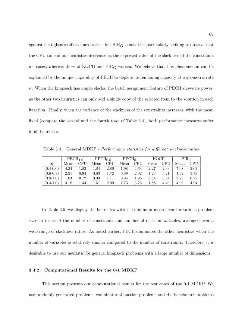
69
against the tightness of slackness ratios, but PIRG is not. It is particularly striking to observe that
the CPU time of our heuristics decreases as the expected value of the slackness of the constraints
increases, whereas those of KOCH and PIRG worsen. We believe that this phenomenon can be
explained by the unique capability of PECH to deplete its remaining capacity at a geometric rate
α. When the knapsack has ample slacks, the batch assignment feature of PECH shows its power,
as the other two heuristics can only add a single copy of the selected item to the solution in each
iteration. Finally, when the variance of the slackness of the constraints increases, with the mean
fixed (compare the second and the fourth rows of Table 3.4), both performance measures suffer
in all heuristics.
Table 3.4. General MDKP - Performance statistics for different slackness ratios
PECH1.0 PECH0.5 PECH0.1 KOCH PIRGSi Mean CPU Mean CPU Mean CPU Mean CPU Mean CPU
(0.4-0.6) 4.24 1.82 1.84 2.86 1.98 4.63 2.27 2.33 7.08 2.63(0.6-0.8) 2.21 0.94 0.83 1.72 0.89 2.82 1.28 3.21 4.32 3.79(0.8-1.0) 1.03 0.72 0.33 1.11 0.34 1.95 0.64 5.54 2.23 6.72(0.4-1.0) 3.18 1.44 1.51 2.00 1.73 3.76 1.88 4.49 4.92 4.94
In Table 3.5, we display the heuristics with the minimum mean error for various problem
sizes in terms of the number of constraints and number of decision variables, averaged over a
wide range of slackness ratios. As noted earlier, PECH dominates the other heuristics when the
number of variables is relatively smaller compared to the number of constraints. Therefore, it is
desirable to use our heuristic for general knapsack problems with a large number of dimensions.
3.4.2 Computational Results for the 0-1 MDKP
This section presents our computational results for the test cases of the 0-1 MDKP. We
use randomly generated problems, combinatorial auction problems and the benchmark problems
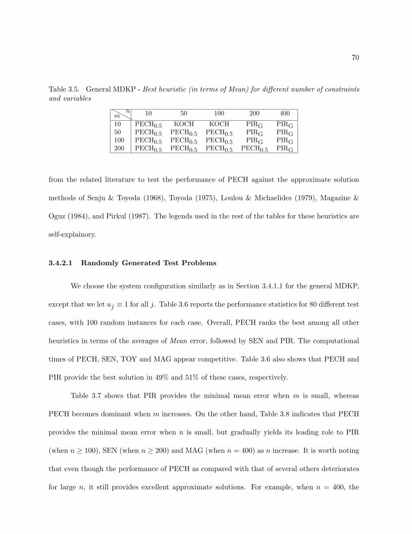
70
Table 3.5. General MDKP - Best heuristic (in terms of Mean) for different number of constraintsand variables
mnHHH
10 50 100 200 400
10 PECH0.5 KOCH KOCH PIRG PIRG50 PECH0.5 PECH0.5 PECH0.5 PIRG PIRG100 PECH0.5 PECH0.5 PECH0.5 PIRG PIRG200 PECH0.5 PECH0.5 PECH0.5 PECH0.5 PIRG
from the related literature to test the performance of PECH against the approximate solution
methods of Senju & Toyoda (1968), Toyoda (1975), Loulou & Michaelides (1979), Magazine &
Oguz (1984), and Pirkul (1987). The legends used in the rest of the tables for these heuristics are
self-explainory.
3.4.2.1 Randomly Generated Test Problems
We choose the system configuration similarly as in Section 3.4.1.1 for the general MDKP,
except that we let uj ≡ 1 for all j. Table 3.6 reports the performance statistics for 80 different test
cases, with 100 random instances for each case. Overall, PECH ranks the best among all other
heuristics in terms of the averages of Mean error, followed by SEN and PIR. The computational
times of PECH, SEN, TOY and MAG appear competitive. Table 3.6 also shows that PECH and
PIR provide the best solution in 49% and 51% of these cases, respectively.
Table 3.7 shows that PIR provides the minimal mean error when m is small, whereas
PECH becomes dominant when m increases. On the other hand, Table 3.8 indicates that PECH
provides the minimal mean error when n is small, but gradually yields its leading role to PIR
(when n ≥ 100), SEN (when n ≥ 200) and MAG (when n = 400) as n increase. It is worth noting
that even though the performance of PECH as compared with that of several others deteriorates
for large n, it still provides excellent approximate solutions. For example, when n = 400, the

71
mean errors of the best heuristic, PIR, and PECH are 0.32% and 0.78%, respectively. Table 3.9
shows that PECH outperforms all other heuristics both in terms of solution quality and CPU
against all levels of the slackness ratio. The robustness of PECH is particularly striking since it
is primarily designed to solve the general MDKP.
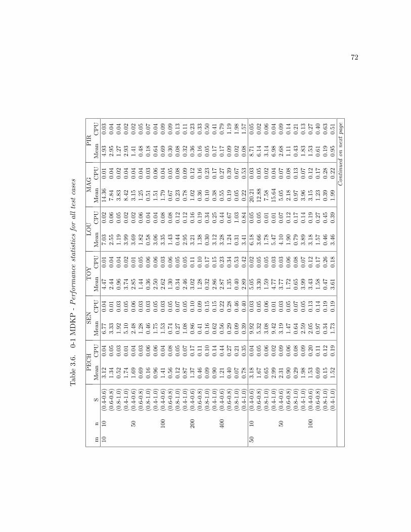
72
Tab
le3.
6.0-
1M
DK
P-Per
form
ance
stat
istics
for
allte
stca
ses
PE
CH
SE
NT
OY
LO
UM
AG
PIR
mn
SM
ean
CP
UM
ean
CP
UM
ean
CP
UM
ean
CP
UM
ean
CP
UM
ean
CP
U
10
10
(0.4
-0.6
)3.1
20.0
46.7
70.0
44.4
70.0
17.0
30.0
214.3
60.0
14.9
30.0
3(0
.6-0
.8)
1.3
40.0
53.3
30.0
12.4
40.0
42.5
50.0
67.8
40.0
42.9
50.0
4(0
.8-1
.0)
0.5
20.0
31.9
20.0
30.9
60.0
41.1
90.0
53.8
30.0
21.2
70.0
4(0
.4-1
.0)
1.7
40.0
15.1
00.0
53.7
40.0
23.9
90.0
28.4
20.0
42.9
30.0
250
(0.4
-0.6
)1.6
90.0
42.4
80.0
62.8
50.0
13.6
90.0
23.1
50.0
41.4
10.0
2(0
.6-0
.8)
0.6
90.0
31.2
80.0
31.4
40.0
51.8
20.0
61.2
50.0
40.4
80.0
5(0
.8-1
.0)
0.1
60.0
60.4
60.0
30.3
60.0
60.5
80.0
40.5
10.0
30.1
80.0
7(0
.4-1
.0)
0.9
60.0
61.7
50.0
52.5
00.0
63.0
60.0
41.5
10.0
60.6
40.0
4100
(0.4
-0.6
)1.4
10.0
41.5
30.0
32.6
20.0
33.3
50.0
81.7
90.0
40.6
90.0
9(0
.6-0
.8)
0.5
60.0
80.7
40.0
51.3
00.0
61.4
30.0
80.6
70.0
50.3
00.0
9(0
.8-1
.0)
0.1
20.0
50.2
70.0
70.3
40.0
50.4
40.1
20.2
30.0
80.0
80.1
3(0
.4-1
.0)
0.8
70.0
71.0
80.0
52.4
60.0
52.9
50.1
20.7
80.0
90.3
20.1
1200
(0.4
-0.6
)1.3
70.1
70.8
60.1
03.0
20.1
13.2
10.1
61.0
20.1
20.3
60.2
3(0
.6-0
.8)
0.4
60.1
10.4
10.0
91.2
80.1
01.3
80.1
90.3
60.1
60.1
60.3
3(0
.8-1
.0)
0.0
90.1
00.1
60.1
50.3
20.1
70.3
00.3
40.1
00.2
30.0
50.5
0(0
.4-1
.0)
0.9
00.1
40.6
20.1
52.8
60.1
53.1
20.2
50.3
80.1
70.1
70.4
1400
(0.4
-0.6
)1.2
10.4
40.5
60.2
22.8
70.2
33.2
80.4
40.5
50.2
70.1
70.7
9(0
.6-0
.8)
0.4
00.2
70.2
90.2
81.3
50.3
41.2
40.6
70.1
90.3
90.0
91.1
9(0
.8-1
.0)
0.0
70.2
10.0
90.4
60.4
00.5
30.3
11.0
30.0
50.6
70.0
21.9
8(0
.4-1
.0)
0.7
80.3
50.3
90.4
02.8
90.4
23.4
10.8
40.2
20.5
30.0
81.5
7
50
10
(0.4
-0.6
)3.1
80.0
49.9
20.0
35.0
50.0
26.1
80.0
520.2
10.0
38.7
10.0
5(0
.6-0
.8)
1.6
70.0
55.3
20.0
53.3
00.0
53.6
60.0
512.8
80.0
56.1
40.0
2(0
.8-1
.0)
0.6
50.0
63.0
80.0
61.5
90.0
51.7
80.0
17.5
80.0
23.1
40.0
6(0
.4-1
.0)
2.9
90.0
29.4
20.0
14.7
70.0
35.4
70.0
115.6
40.0
46.9
80.0
450
(0.4
-0.6
)2.3
10.0
93.1
90.0
33.7
70.0
34.1
00.0
75.0
50.0
72.6
80.0
9(0
.6-0
.8)
0.9
00.0
61.4
70.0
51.7
20.0
61.9
00.1
22.1
80.0
81.1
10.1
4(0
.8-1
.0)
0.2
90.0
80.6
40.0
70.6
50.0
80.7
90.1
70.9
70.1
30.4
30.2
1(0
.4-1
.0)
1.9
80.0
92.5
90.0
53.9
90.0
73.8
90.1
43.9
60.0
71.8
30.1
3100
(0.4
-0.6
)1.5
30.2
02.0
50.1
33.4
30.1
23.1
80.1
93.1
50.1
21.5
30.2
7(0
.6-0
.8)
0.6
90.1
10.9
70.1
41.5
80.1
71.5
70.2
71.2
30.1
70.6
10.4
0(0
.8-1
.0)
0.1
50.1
20.3
40.1
90.4
70.2
60.4
60.4
50.3
90.2
80.1
90.6
3(0
.4-1
.0)
1.5
20.1
91.7
30.1
93.6
10.1
83.4
60.3
91.9
90.2
20.9
50.5
1
Continued
on
nex
tpa
ge
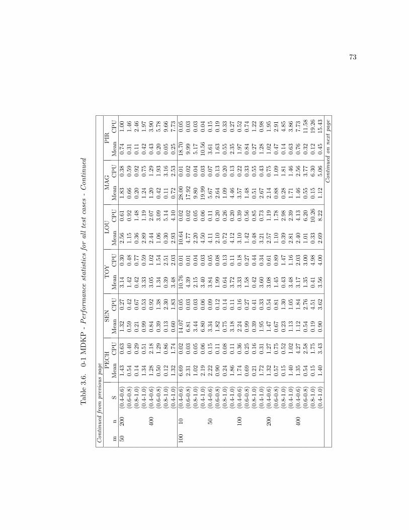
73
Tab
le3.
6.0-
1M
DK
P-Per
form
ance
stat
istics
for
allte
stca
ses
-C
ontinu
ed
Continued
from
pre
vious
page P
EC
HSE
NT
OY
LO
UM
AG
PIR
mn
SM
ean
CP
UM
ean
CP
UM
ean
CP
UM
ean
CP
UM
ean
CP
UM
ean
CP
U
50
200
(0.4
-0.6
)1.4
30.6
31.3
20.2
73.1
40.3
02.5
60.6
11.8
30.3
80.7
41.0
0(0
.6-0
.8)
0.5
40.4
00.5
90.4
21.4
20.4
81.1
50.9
20.6
60.5
90.3
11.4
6(0
.8-1
.0)
0.1
40.2
90.2
10.6
70.4
20.7
70.3
61.4
80.2
00.9
20.1
12.4
6(0
.4-1
.0)
1.3
40.5
10.9
90.5
33.3
30.5
92.8
91.1
91.2
40.7
50.4
21.9
7400
(0.4
-0.6
)1.2
82.1
80.8
40.9
23.0
51.0
22.4
42.0
71.2
01.2
90.4
33.9
0(0
.6-0
.8)
0.5
01.2
90.3
91.3
81.3
41.5
41.0
63.0
90.4
21.9
30.2
05.7
8(0
.8-1
.0)
0.1
20.8
60.1
32.3
00.3
92.5
10.3
05.1
40.1
13.1
60.0
59.6
6(0
.4-1
.0)
1.3
21.7
40.6
01.8
33.4
82.0
32.9
34.1
00.7
22.5
30.2
57.7
3
100
10
(0.4
-0.6
)6.6
90.0
214.0
70.0
510.7
60.0
110.6
40.0
228.0
00.0
118.7
00.0
5(0
.6-0
.8)
2.3
10.0
36.8
10.0
34.3
90.0
14.7
70.0
217.9
20.0
29.9
90.0
3(0
.8-1
.0)
1.0
20.0
53.4
40.0
32.1
50.0
42.2
00.0
59.8
00.0
45.1
70.0
3(0
.4-1
.0)
2.1
90.0
66.8
00.0
63.4
00.0
34.5
00.0
619.9
90.0
310.5
60.0
450
(0.4
-0.6
)2.2
20.1
53.3
40.0
93.8
40.0
54.1
10.1
15.6
70.0
73.6
10.1
5(0
.6-0
.8)
0.9
00.1
11.8
20.1
21.9
90.0
82.1
00.2
02.6
40.1
31.6
30.1
9(0
.8-1
.0)
0.2
40.0
80.7
50.1
40.6
40.1
30.7
20.2
61.0
90.2
00.5
50.3
3(0
.4-1
.0)
1.8
60.1
13.1
80.1
13.7
20.1
14.1
20.2
04.4
60.1
32.3
50.2
7100
(0.4
-0.6
)1.7
40.3
62.2
40.1
63.3
30.1
83.1
00.3
93.5
70.2
21.9
70.5
2(0
.6-0
.8)
0.6
90.2
50.9
90.2
71.5
80.2
71.4
20.5
61.4
80.3
30.8
40.7
4(0
.8-1
.0)
0.2
10.1
60.3
90.4
10.4
20.4
40.4
80.8
50.5
10.5
50.2
71.2
2(0
.4-1
.0)
1.7
20.3
11.9
50.3
33.6
00.3
43.2
10.7
32.6
70.4
31.2
80.9
8200
(0.4
-0.6
)1.3
21.2
71.4
70.5
43.0
80.6
12.5
71.1
92.1
40.7
51.0
21.9
5(0
.6-0
.8)
0.5
70.7
50.6
70.8
11.4
50.8
91.1
01.7
80.8
81.0
90.4
72.9
1(0
.8-1
.0)
0.1
50.5
20.2
31.3
00.4
31.4
70.3
92.9
80.2
81.8
10.1
44.8
5(0
.4-1
.0)
1.4
01.0
21.1
31.0
53.4
81.1
62.8
12.3
91.7
11.4
60.6
33.8
6400
(0.4
-0.6
)1.3
54.2
71.1
21.8
43.1
72.0
32.4
04.1
31.4
62.5
60.7
67.7
3(0
.6-0
.8)
0.5
42.5
80.5
42.7
61.3
53.0
01.0
16.2
00.5
53.7
70.3
211.5
8(0
.8-1
.0)
0.1
51.7
50.1
94.5
10.4
14.9
80.3
310.2
60.1
56.3
00.1
219.2
6(0
.4-1
.0)
1.4
03.4
30.9
03.6
23.5
64.0
02.6
98.2
21.1
25.0
60.4
515.4
3
Continued
on
nex
tpa
ge

74
Tab
le3.
6.0-
1M
DK
P-Per
form
ance
stat
istics
for
allte
stca
ses
-C
ontinu
ed
Continued
from
pre
vious
page P
EC
HSE
NT
OY
LO
UM
AG
PIR
mn
SM
ean
CP
UM
ean
CP
UM
ean
CP
UM
ean
CP
UM
ean
CP
UM
ean
CP
U
200
10
(0.4
-0.6
)23.7
70.0
532.3
30.0
130.8
00.0
630.6
70.0
534.8
60.0
544.9
90.0
2(0
.6-0
.8)
12.4
30.0
319.3
20.0
417.0
80.0
517.6
80.0
418.8
20.0
425.5
80.0
5(0
.8-1
.0)
6.7
50.0
511.4
00.0
410.2
10.0
79.8
60.0
511.6
00.0
414.7
10.0
4(0
.4-1
.0)
17.3
90.0
627.1
50.0
523.3
30.0
624.6
30.0
724.5
40.0
428.0
10.0
750
(0.4
-0.6
)4.3
90.2
56.6
00.1
36.7
30.1
47.1
50.2
46.7
80.1
47.6
80.2
9(0
.6-0
.8)
2.0
30.1
43.3
90.1
43.4
00.1
83.5
90.3
12.8
70.2
03.2
20.4
0(0
.8-1
.0)
0.6
70.1
01.3
70.2
31.1
50.2
71.3
00.5
21.1
60.3
51.2
30.6
4(0
.4-1
.0)
3.7
10.2
05.3
30.1
96.4
50.2
26.3
20.4
15.5
90.2
75.4
20.5
2100
(0.4
-0.6
)2.6
10.7
43.6
50.3
34.8
10.3
64.2
20.7
03.7
30.4
53.5
60.9
8(0
.6-0
.8)
1.1
10.4
31.6
60.4
72.1
20.5
41.9
91.0
31.7
30.6
61.5
01.4
9(0
.8-1
.0)
0.4
20.3
20.6
50.7
50.7
50.8
40.8
31.7
40.5
81.0
40.5
92.4
4(0
.4-1
.0)
2.4
60.6
13.1
80.6
34.6
00.6
84.1
81.4
03.0
20.8
82.4
31.9
8200
(0.4
-0.6
)1.6
82.4
62.0
41.0
73.7
11.1
92.9
82.4
02.4
01.4
71.9
13.8
6(0
.6-0
.8)
0.7
91.5
21.0
11.5
91.6
31.7
61.3
63.5
41.0
52.1
80.8
05.7
8(0
.8-1
.0)
0.2
41.0
30.3
72.6
40.5
02.9
00.4
85.9
10.3
43.6
10.2
99.6
8(0
.4-1
.0)
1.7
42.0
11.7
52.0
93.9
72.3
23.0
84.7
51.9
92.9
01.2
27.7
2400
(0.4
-0.6
)1.3
38.5
81.2
53.6
33.0
14.0
31.8
78.2
51.7
05.0
21.0
015.4
3(0
.6-0
.8)
0.5
45.1
30.6
15.4
51.2
56.0
11.1
312.3
00.6
57.5
60.4
223.1
1(0
.8-1
.0)
0.1
63.4
30.2
19.0
30.4
19.9
60.3
120.5
30.1
912.5
60.1
538.5
2(0
.4-1
.0)
1.3
86.8
31.0
07.2
33.3
97.9
81.6
716.4
41.3
910.0
50.6
730.8
4
Averag
e1.9
70.7
83.1
50.8
23.4
60.9
03.4
81.8
34.5
01.1
33.2
53.2
5

75
Table 3.7. 0-1 MDKP - Performance statistics for different number of resource constraints
PECH SEN TOY LOU MAG PIRm Mean CPU Mean CPU Mean CPU Mean CPU Mean CPU Mean CPU10 0.92 0.12 1.50 0.12 2.02 0.13 2.42 0.23 2.36 0.15 0.86 0.3950 1.23 0.45 2.29 0.47 2.53 0.52 2.51 1.03 4.08 0.64 1.84 1.83100 1.43 0.86 2.60 0.91 2.84 0.99 2.73 2.03 5.30 1.25 3.04 3.61200 4.28 1.70 6.21 1.79 6.47 1.98 6.27 4.03 6.25 2.48 7.27 7.19
Table 3.10 presents the heuristics with the minimum mean error for various problem sizes in
terms of the number of constraints and number of decision variables. Clearly, PECH outperforms
the other heuristics when the number of constraints are relatively larger than the number of
variables, which can be observed in the lower triangle region of the table.
3.4.2.2 Benchmark Problems from the Literature
We solve two capital budgeting problems taken from Weingartner & Ness (1967), two others
from Petersen (1967) and two resource planning problems from Senju & Toyoda (1968). These six
problems have been used extensively as the benchmark problems in the existing literature to test
the effectiveness of proposed heuristics. We report the optimal solution and the heuristic solutions
for each problem in Table 3.11. The results for SEN, TOY, LOU and MAG are taken from their
respective references, and the results for PECH and PIR are based on our own computations.
Table 3.11 indicates that the maximum deviation of the solution by PECH from the optimal
solution is only 1.29%. In the remaining five problems, the deviation is much smaller then 1%.
PECH provides the best solution in two of these problems and the second best solution in another
two. The closest competitor of PECH is PIR, which requires to solve a linear program and hence
needs a larger CPU. Therefore, we conclude that our heuristic manages these benchmark problems
aptly.

76
Table 3.8. 0-1 MDKP - Performance statistics for different number of decision variables
PECH SEN TOY LOU MAG PIRn Mean CPU Mean CPU Mean CPU Mean CPU Mean CPU Mean CPU10 5.49 0.04 10.39 0.04 8.03 0.04 8.55 0.04 16.02 0.03 12.17 0.0450 1.56 0.10 2.48 0.10 2.83 0.10 3.08 0.18 3.05 0.13 2.15 0.22100 1.11 0.25 1.46 0.26 2.31 0.29 2.27 0.57 1.72 0.35 1.07 0.79200 0.89 0.81 0.86 0.84 2.13 0.94 1.86 1.88 1.04 1.16 0.55 3.06400 0.78 2.71 0.57 2.87 2.02 3.16 1.65 6.48 0.67 3.98 0.32 12.16
Table 3.9. 0-1 MDKP - Performance statistics for different slackness ratios
PECH SEN TOY LOU MAG PIRSi Mean CPU Mean CPU Mean CPU Mean CPU Mean CPU Mean CPU
(0.4-0.6) 3.28 1.10 4.88 0.48 5.38 0.53 5.44 1.06 7.13 0.66 5.34 1.87(0.6-0.8) 1.48 0.67 2.58 0.71 2.67 0.78 2.70 1.57 3.81 0.97 2.86 2.79(0.8-1.0) 0.62 0.47 1.32 1.16 1.15 1.28 1.17 2.60 1.98 1.60 1.44 4.64(0.4-1.0) 2.48 0.89 3.83 0.93 4.66 1.03 4.62 2.09 5.07 1.29 3.38 3.71
Table 3.10. 0-1 MDKP - Best heuristic (in terms of Mean) for different number of constraintsand variables
mnHHH
10 50 100 200 400
10 PECH PIR PIR PIR PIR50 PECH PECH PIR PIR PIR100 PECH PECH PECH PIR PIR200 PECH PECH PECH PECH PIR

77
Table 3.11. Optimal and heuristic solutions of six 0-1 MDKP from literature
Problem m n Z∗ ZPECH ZSEN ZTOY ZLOU ZMAG ZPIRWeingartner & Ness (1967)1 2 28 141,278 140,618 138,888 139,278 135,673 139,418 140,4772 2 105 1,095,445 1,094,262 1,093,181 1,088,365 1,083,086 1,092,971 1,094,757Petersen (1967)1 5 39 10,618 10,480 9,548 10,320 9,290 10,354 10,5472 5 50 16,537 16,463 16,237 15,897 14,553 16,261 16,436Senju & Toyoda (1968)1 30 60 7,772 7,700 7,590 7,719 7,675 7,719 7,7282 30 60 8,722 8,666 8,638 8,709 8,563 8,623 8,697
3.4.2.3 Combinatorial Auction Problems
Auctions where bidders submit bids on bundles of items, instead of only on individual
items, are called combinatorial auctions (de Vries & Vokra 2001). Combinatorial auctions have
received great attention from researchers due to their wide applicability in practice, such as FCC
auctions of spectrum rights, auctions for airport time slots, procurement of logistics services
and network routing. A combinatorial auction problem is often a large-scale integer program
problem, with at least hundreds of decision variables (bids) and constraints (items). The problem
of identifying which set of bids to accept is known as the winner determination problem. The
winner determination problem for multi-unit combinatorial auctions, where there are multiple
units of the same item available and bidders may want more than one unit of the same item, can
be formulated as an integer program as follows. Consider a combinatorial auction where n bidders
are bidding for m different items. Each bidder requires a subset of items, possibly multiple units
of each, in his/her bundle. Let aij be the number of units of item i included in the bundle of
bidder j, i = 1, . . . ,m, j = 1, . . . , n. Denote bi as the number of copies of item i, i = 1, 2, . . . , m,
78
to be auctioned. The seller receives cj , if bidder j wins the auction. It is clear that the seller’s
winner determination problem is equivalent to a 0-1 MDKP.
Exact solution methods for combinatorial auction problems are based on branch and bound,
cutting planes, and branch and cut algorithms. Since standard commercial math programming
packages, such as Cplex, run into storage (memory) problems, a number of specialized software
packages have been developed for these auctions (OptiBid by Logistics.com, SBID by SAITECH-
INC). Furthermore, Fujishima, Leyton-Brown & Shoham (1999) and Sandholm (1999) have pro-
posed dynamic programming-based exact methods. On the other hand, a very large number of
approximate methods have been applied to the combinatorial auction problems, ranging from the
very simple greedy algorithms (Fisher & Wolsey 1982) to more complicated genetic algorithms
(Huang, Kao & Hong 1994), probabilistic search (Feo, Mauricio & Resende 1989), and neural
networks (Aourid & Kaminska 1994).
In order to create benchmark auctions, Sandholm (1999) proposed the following distribu-
tions to generate bids in a given auction:
• Random: For each bid, we pick the number of items randomly from 1, 2, ..., m. Then we
randomly choose that many items without replacement and pick a price from [0,1]. The
number of units of each item selected in the bid is generated using a discrete distribution.
• Weighted Random: This is very similar to Random, but we pick a price between 0 and the
number of items in the bid.
• Uniform: For each bid, we select the same number of randomly chosen items and pick a
price from [0,1]. The number of units of each item selected in the bid is generated using a
discrete distribution.

79
• Decay : We start with one random item in a bid and then repeatedly add a new item with
probability δ until an item is not added or the bid includes all m items (we set δ = 0.75).
We pick a price between 0 and the number of items in the bid. The number of units of each
item selected in the bid is generated using a discrete distribution.
Based on each generating scheme described above, we study 20 randomly generated auc-
tions with 2000 items and 100 bidders. The number of copies of each item available in the auction
is generated using the concept of slackness ratio Si, described in (3.11). We let Si ∼ Unif(0.1, 0.3)
and Si ∼ Unif(0.3, 0.5) for two levels of constraint tightness.
Here, we solve the linear programming relaxation of the integer program corresponding to
the 0-1 MDKP, since the exact solutions of these large-scale combinatorial auction problems using
Cplex are computationally inefficient. Notice that the proposed relaxation constitutes an upper
bound on the optimal solution of the problem. We report the average error of each heuristic based
on this bound over 20 instances of each auction in Table 3.12.
Table 3.12. Computational Results for Combinatorial Auction Problems
Bid Distribution Si PECH SEN TOY LOU MAG PIRRand (0.1-0.3) 0.43 0.48 1.1 0.73 0.52 0.21
(0.3-0.5) 0.26 0.31 0.76 0.45 0.45 0.12Wrand (0.1,0.3) 0.46 0.50 1.15 0.75 0.53 0.24
(0.3,0.5) 0.28 0.36 0.77 0.47 0.49 0.14Unif (0.1,0.3) 0.49 0.54 1.16 0.80 0.55 0.25
(0.3,0.5) 0.29 0.38 0.79 0.51 0.51 0.15Decay (0.1,0.3) 0.53 0.58 1.19 0.84 0.59 0.30(δ = 0.75) (0.3,0.5) 0.32 0.43 0.81 0.54 0.52 0.18
Average 0.35 0.40 0.93 0.59 0.49 0.17
We mentioned previously that Pirkul’s algorithm dominates our heuristic when the number
of decision variables is large. Our computational results for the randomly generated combinatorial
auction problems support this observation. PIR deviates from the upper bound by 0.17% on
80
average, whereas PECH by 0.40%. However, PECH is the best heuristic among the greedy
algorithms. Further, as the tightness of the resource constraints decreases, the performances of
all heuristics significantly improve.
3.5 Conclusion
In this essay, we further investigate the analytical properties and computational effective-
ness of the heuristic we introduced in Chapter 2. The intuition behind our heuristic is entirely
different from those of greedy-like solution methods. Instead of using a criterion based on each
item’s aggregate consumption of the resources, our heuristic uses the notion of effective capacity,
defined as the maximum number of copies of an item that can be accepted if the entire knapsack
were to be used for that item alone. Furthermore, our heuristic includes the selected items in the
solution in batches, which consequently improves computational effort. Although our heuristic is
primarily design for the general MDKP, it also solves the 0-1 version of the problem effectively.
The numerical results on a large number of randomly generated problem instances for both the
general MDKP and 0-1 MDKP demonstrate the superiority/competitiveness of our heuristics
against other existing ones. Other computations based on assemble-to-order manufacturing sys-
tems (presented in Chapter 2), combinatorial auctions, and the benchmark problems from the
literature support the strength of our heuristics and its trustworthy for real-time implementations.

81
Chapter 4
ONLINE ASSIGNMENT OF FLEXIBLE RESOURCES
4.1 Introduction
Flexibility is the ability of an operation to cope with changes effectively by allowing the
system to use its resources to process different types of products. In today’s ever-changing busi-
ness environment, fuelled by the burden of market responsiveness, competition, shorter product
life cycles, and availability of new technologies, flexibility has become a vital facet of both man-
ufacturing and service operations by guarding these systems against uncertainty. Consequently,
flexibility is considered indispensable to the extent that it should be a part of the competitive
strategy. Indeed, a survey of over 500 manufacturing corporations reveals that flexibility is ranked
right after productivity, delivery and quality in importance for competitiveness (DeMeyer, Nakane,
Miller & Ferdows 1987). Today, strategic significance of flexibility is well understood by decision
makers, and earlier beliefs that it is “a neglected aspect of behavior under risk when faced with
uncertainty” are overhauled (Jones & Ostroy 1984). However, strategic and operational decisions
of flexibility have to be integrated in order to fully realize the benefits of flexibility.
At the strategic level, the focus is on the role of flexibility in handling uncertainties. Flex-
ibility requirements are translated into capacity and performance objectives. This area has been
a popular research field due to the emergence of related technologies. Fine & Freund (1990)
investigate the capacity planning problem for a flexible manufacturing system, and identify the
necessary and sufficient conditions for a firm to invest in flexible capacity to protect against
uncertainty in demand for all of its products. Their model assesses cost/benefit trade-offs for

82
investment in product-flexible manufacturing systems. In a closely related work, Mieghem (1998)
uses his descriptive model to deliver additional intuitions on investment decisions and the value
of flexibility. Jordan & Graves (1995) develop principles on how much flexibility is needed and
how to add flexibility to an existing system. They state that limited flexibility configured in the
right way can have the benefits of total flexibility, and propose a “chain” structure as an effective
mechanism to create flexibility.
On the other hand, at the operational level, concern is with designing specific methods of
delivery and deployment of flexibility. Once flexibility is adopted, the decision maker faces the
problem of effectively allocating flexibility to various operations in order to achieve the goals set
at the strategic level. In this essay, we investigate the dynamic allocation of flexible resources at
the operational level. In other words, for a given set of resources, whose capacity and flexibility
decisions are already made at the strategic level, we explore mechanisms to assign them to different
products, so as to effectively handle the demand uncertainty for these products. The dynamic
nature of the problem arises because of the fact that product demands arrive over a finite time
horizon and resources are committed upon arrival to process the products at the end of the
time horizon. These features enable the practice of revenue management in this dynamic flexible
resource allocation problem.
Airlines, lodging and hospitality, automobile rental, and many other service industries, are
challenged with the problem of supplying their customers from a fixed inventory of resources over
a finite period of time. Revenue management is a business practice to maximize profits by selling
these resources to the right customer, at the right price and at the right time, and has been a
very powerful managerial tool in exploiting the potential of increased revenues in many businesses
83
(Cross 1997, Belobaba 1989, Smith, Leimkuhler & Darrow 1992). The widely publicized applica-
tions of airline revenue management inspired the development of revenue management systems in
other service industries. Regardless of the application area, revenue management problems share
four common features - resources become extinct (or perish) after a certain deadline, inventory of
available resources during the planning horizon is fixed (or almost impossible to replenish within
the duration of the planning horizon), demand for these resources is stochastic, and multiple types
of resources can potentially satisfy a given customer demand. Weatherford & Bodily (1992) unified
different management practices with the aforementioned characteristics under the perishable-asset
revenue management (PARM) taxonomy. PARM attempts to determine the array of resources
to be made available initially at various price levels and the dynamics of this availability over
time. The decision-maker can evaluate his strategic choices through various metrics, including
total profit, total revenue, average revenue per customer, capacity utilization, and lost customer
goodwill. While the decision-maker can focus on any of these metrics, the fundamental decisions
are whether or not to accept a customer request, and which resource to assign to an accepted
request. The problem is complex since these decisions must be reached almost immediately, and
all possible future realizations of customer demand and currently available inventory should be
taken into account. Therefore, a full assessment of each individual request in real time is almost
impossible, especially in large systems.
In this essay, we set our problem in a workplace learning industry context. The connec-
tion between rapid technological change and the emergence of global economy have created the
necessity for profound changes in the way people and organizations work. However, workplace
learning remains the powerhouse of building corporate success and is probably more strategic to
the competitive advantage of both individuals and employers than at any point in recent years.

84
Being a significant supplier of education, news and skill development for businesses, workplace
learning industry has been growing rapidly as a result of these developments. Indeed, according
to the 2002 International Comparisons Report of the American Society for Training Development
(ASTD), the percentage of employees who received training, in more than 550 organizations from
42 countries, was 76.7% in 2000, compared to 74.9% in 1999 and 67.6% in 1998. Similarly, the
training expenditures of organizations as a percentage of their total annual payrolls increased
from 1.8% in 1997 to 2.5% in 2000. Organizations spent an average of $630 per employee on
training in 2000, and this amount is projected to continue its upward trend in upcoming years.
On a global scale, organizations devoted an average of 26.2% of their total training expenditures
to outsourced training in 2000.
We consider a workplace learning provider (WLP), offering various types of training pro-
grams to its clients. These clients are corporations seeking outsourced training for their employees.
The WLP utilizes instructor-led classroom as its method of training delivery. Although, this tech-
nique might appear outdated at first, it is still the most dominant form according to the 2002
report of the ASTD, which associates this trend with the recent decline of the e-learning market-
place. Instructors employed by the WLP have different capabilities based on their qualifications
- some of them are specialized to teach only one particular type of training program, whereas
others are experienced enough to teach multiple. This distinction introduces resource flexibility
to the problem context. In other words, the decision-maker has the liberty to assign any one of
the capable instructors to a particular client request. The ultimate goal of the decision-maker is
to maximize the WLPs expected revenues by intelligently utilizing its limited resources to meet
the stochastic demand over the finite planning horizon. At the strategic level, the decision-maker
faces the problem of determining the portfolio of instructors to employ. On the other hand, the

85
operational level accept/reject decisions of client requests and instructor assignment decisions,
that are possibly made online (immediately when the request arrives), fall into the realm of rev-
enue management, and are our main interest in this essay. If a current request is accepted, the
decision-maker gives up the opportunity to use the assigned instructor for a potentially more prof-
itable future request. Then again, if the request is rejected, there is a risk of having to assign the
instructor to a less profitable request or even being left with an idle instructor at the end of the
planning horizon. In fact, these are the tradeoffs that lead to the potential of exercising revenue
management practices in this context. This problem is significantly different than most revenue
management applications. An airline revenue management problem is complex because of the
frequency of decisions made for millions of customers in very short periods of time. Although, our
problem does not have this property, the complexity of the resource structure makes the problem
challenging.
We model the workplace learning revenue management problem as a stochastic dynamic
program. The optimal policy could ideally be found by solving the associated Bellman equation,
using backward induction. However, this technique is computationally inefficient because of the
large state space of the problem (curse of dimensionality). Therefore, researchers have focused on
approximate solution methods and structural properties of the optimal policy instead. Likewise,
we propose several heuristics to solve the problem, which are based on our analysis of special cases.
We extend the insights gained from this analysis to the general problem, and develop simple, but
effective, solution methods, verified through a comprehensive computational study. Our results
show the average difference between our best heuristic solution and the optimal solution is much
less than 1% in most cases. Our contributions in this essay are three-fold: we propose new models
for a new application area and present effective procedures as approximate solution methods.

86
The rest of this essay is organized as follows: We review the revenue management literature
in Section 4.2. In Section 4.3, we formally define our model and formulate it as a stochastic
dynamic program. We analyze four special cases of the problem in Section 4.4. Based on these
initial results, we propose heuristic solution methods in Section 4.5. In Section 4.6 we report our
computational results for the problem. Finally, conclusions and a discussion of future research is
presented in Section 4.7.
4.2 Review of Revenue Management Literature
Research in the field of revenue management starts with the study of a two-class, single-
leg airline seat allocation problem by Littlewood (1972). Alstrup, Boas, Madsen & Vidal (1986)
consider an overbooking model for the same problem, and Belobaba (1989) introduces the expected
marginal seat revenue (EMSR) heuristic for the more general multi-class setting. EMSR withholds
seats for each customer class in such a way that the marginal revenue generated from sales to
a higher paying class would be exactly equal to the fare of that class. These booking limits are
revised dynamically over time as customer demand is realized. Wollmer (1992) and Brumelle
& McGill (1993) study similar nested multi-class, single-leg problems and prove that EMSR
allocates non-optimal seat reservations, though the difference with the optimal policy is usually
small. Therefore, they use variations of the EMSR model to guide their own heuristic solutions.
van Ryzin & McGill (2000) employ historical observations of the relative frequencies of certain
seat-filling events to adjust booking limits, based on the optimality conditions of Brumelle &
McGill (1993), and show that their adaptive solution converges to the optimal.
Simpson (1989) and Williamson (1992) propose the bid price control (BPC) heuristic to
solve the multi-leg version of the problem, which they model as a static network. They use

87
deterministic mathematical programming models to estimate the opportunity cost of each leg,
and simply add these costs to find the value of an itinerary (collection of legs). Using a general
model of demand, Talluri & Ryzin (1999) prove that BPC is not optimal for general dynamic
networks and investigate why it fails to produce optimal decisions. Bertsimas & Popescu (2001)
introduce the certainty equivalent control (CEC) heuristic, based on an approximate dynamic
programming model. They report that their algorithm is superior to BPC in terms of revenue
generation and robustness.
Bitran & Mondschein (1995) and Bitran & Gilbert (1996) study optimal strategies for rent-
ing hotel rooms in the presence of stochastic arrival of customers from different market segments,
and model the problem as a stochastic dynamic program, similar to Bertsimas & Popescu (2001).
Gallego & Ryzin (1994) address a revenue management problem for a fashion producer-retailer,
but focus on the dynamic pricing of inventory, rather than inventory allocation. Feng & Gallego
(1995) analyze the timing of price reductions for end-of-sales and optimal stopping times of such
promotional prices. Feng & Xiao (1999) and Feng & Xiao (2000) incorporate a risk factor into
the model and extend the previous results to deal with multiple price changes.
Other applications of revenue management include automobile rental (Geraghty & Johnson
1997, Carroll & Grimes 1995), cruise lines (Ladany & Arbel 1991, Gallego & Ryzin 1994), and
railways (Strasser 1996, Ciancimino, Inzerillo, Lucidi & Palagi 1999). We refer the reader to
Weatherford & Bodily (1992) and McGill & Ryzin (1999) for extensive surveys of the revenue
management literature.

88
4.3 Problem Definition and Formulation
In this section, we start with a brief description of the revenue management problem in
the workplace learning industry context. We build a general framework that would be helpful
for understanding different aspects of the problem and use it to introduce the details. Then,
we provide the notation that we use throughout the essay. Finally, we provide the stochastic
dynamic programming formulation of the problem, and review the literature on approximate
solution methods.
4.3.1 Problem Definition
A workplace learning provider (WLP) offers m different types of training programs to its
clients, and employs ` different types of instructors, such that instructors of the same type have
similar skills and can teach the same set of training programs. This resource structure is described
by an m× ` matrix A. The entry aij of A is equal to 1 if a type-j instructor can teach a type-i
training program; otherwise it is 0. For example, consider a WLP with m = 3 types of training
programs and ` = 7 types of instructors. Suppose that the first training program can be taught
by instructors of types 1, 4, 5 and 7; the second by types 2, 4, 6 and 7; and the third by types 3,
5, 6 and 7. This resource structure is given by:
A =
1 0 0 1 1 0 10 1 0 1 0 1 10 0 1 0 1 1 1
(4.1)
In our discussions, we refer to instructors that can only teach one type of training program
as special-purpose instructors, and the ones that can teach multiple training programs as flexible
instructors. In the above example, type 1, 2 and 3 instructors are special-purpose, whereas type

89
4, 5, 6 and 7 are flexible. Note that type 7 instructors are more flexible than the others, since
they can teach a larger set of training programs.
The net revenue from a type-i training program is πi and is independent of the type of
instructor assigned to teach it. Without loss of generality, assume that π1 ≥ π2 ≥ · · · ≥ πm. The
length of the planning horizon, T , is finite and is traced backwards (t = T is the beginning of the
planning horizon and t = 0 is the end). The number of instructors currently available at time t
is given by the vector nt = (n1t, . . . , n`t). Consequently, the number of instructors employed by
the WLP is nT = (n1T , . . . , n`T ).
The objective of the decision-maker is to maximize the expected total revenue over the
finite planning horizon. In order to achieve this goal, one has to allocate the available but limited
set of resources wisely. There are two major decisions involved in the process. The first is to
decide whether to accept or reject an incoming request from a client (acceptance decision), and
the second is to decide which instructor to assign to an accepted request (assignment decision).
The decision-maker has to consider the future demand, the availability of instructors, relative
monetary returns from offered training programs, among many other things, making the problem
a difficult one to solve.
We now set the following framework to describe different aspects of this revenue man-
agement problem. In order to keep our discussions general, we adopt the term resources for
instructors and jobs for training programs.
Flexibility structure of resources. The WLP determines the flexibility structure and the ini-
tial quantity of resources at the strategic level. However, this structure plays a crucial role
on the decision-maker’s actions at the tactical level during the finite planning horizon. Some
common resource structures are as follows:

90
• Special-purpose resources only : Each type of jobs is handled by a special-purpose re-
source. The solution to this problem is trivial, since there is no risk or opportunity
involved with the acceptance or assignment decisions.
• Full spectrum of resources: For each subset S ⊆ {1, 2, . . . , m}, there exists a resource
type that can only process the job types in S. In this case, 2m − 1 types of resources
should be held to process m different job types. Clearly, this would be the most
complicated resource structure for the decision-maker to handle. The setting given in
equation (4.1) would be an example for such a resource structure.
• A single flexible resource: A single type of flexible resource is used to handle every
types of job. This resource structure is widely adopted in various revenue management
applications. For instance, the same airline seat is used to satisfy the demand from
different market segments. Here, the resource assignment decision is eliminated from
the problem.
• Nested resource structure: A type-j resource, j = 1, 2, . . . , m, is flexible to process all
jobs of types i = 1, 2, . . . , j. In other words, a type-j resource can be assigned to a
type-j job, and also can be used for all lower indexed jobs (higher revenue generating
jobs).
Frequency of decisions. Uncertainty of demand is one of the main reasons for the complexity of
the problem. In order to reduce this uncertainty, the decision-maker might opt for observing
the demand, at least partially, before accepting any client requests or assigning resources.
He achieves this by dividing the time horizon into decision windows and allowing demand
information to accumulate, after which he takes actions. For instance, the decision-maker
can get back to clients about their requests at the end of each day or at the end of each
91
week. Obviously, the longer the decision window, the better decisions he will be able to make.
However, these response delays might hurt the customers’ perception of service quality and
goodwill.
Timing of decisions. The acceptance and assignment decisions can either be made immediately
after the client request is received, or can be deferred until the end of the finite planning
horizon. This dimension of the problem results in the following three scenarios:
• online acceptance and assignment decisions (OO)
• online acceptance decision but deferred assignment decision (OD)
• deferred acceptance and assignment decisions (DD)
Clearly, OO is the most complicated and DD is the easiest for the decision-maker to manage.
Revenue management capitalizes on the ability of adjusting the prices of the services provided,
as much as selecting the right customer to sell those services, in order to maximize revenues.
Primarily, pricing allows the decision-maker to fine-tune the demand arrival process. However,
pricing is not always allowed, particularly in industries for which the price of the service is fixed.
Then, it is the decision-maker’s skill in allocating the resources, that determines the corporate
success.
In this essay, we model the revenue management problem with the following assumptions,
based on our framework:
• We assume that the WLP employs the full spectrum of resources, which is much more
complicated than the common practice in revenue management literature.
• We use a discrete-time model to study the problem.

92
• Both the acceptance and assignment decisions are made online, at the end of each period.
• We do not make any particular assumption about demand distributions, but require de-
mands across time periods to be independent. We also allow batch arrivals to occur in each
period.
• We assume that the decision-maker cannot change the price he charges for each job. There-
fore, our focus is on the resource allocation decisions.
• We do not let a client cancel his request for a job. Similarly, the WLP cannot recall a
resource that has been assigned to a particular client.
We define the problem with these properties as the online assignment of flexible resources problem.
4.3.2 Notation
Here is the notation that we use throughout the essay:
m = number of job types;
` = number of resource types;
i = index for job types, i = 1, 2, . . . , m;
j = index for resource types, j = 1, 2, . . . , `;
T = number of periods in the finite planning horizon;
t = time periods left until the end of the planning horizon;
aij = 1 if type-j resource can be assigned to type-j job, otherwise 0;
ϕj = flexibility index of the type-j resource;
ϕj =m∑
i=1aij
A = {aij}, resource structure matrix;
93
Ji = set of resource types that can be assigned to type-i jobs,
Ji = {j : aij = 1, j = 1, . . . , `};
njt = number of type-j resources available in period t;
nt=(n1t, n2t, . . . , n`t);
πi = revenue collected from a type-i job;
Dit = random demand for the type-i jobs in period t;
Dt = (D1t, D2t, . . . Dmt);
dit = a realization of the random demand for the type-i jobs in period t;
dt = (d1t, d2t, . . . , dmt);
Dit = random aggregate demand for type-i jobs over the remaining t periods;
Dt = (D1t, D2t, . . . , Dmt);
dit = a realization of the random aggregate demand for type-i jobs over the
remaining t periods;
dt = (d1t, d2t, . . . , dmt);
ej = jth unit vector. The dimensionality of ej will depend on the problem
instance.
4.3.3 Problem Formulation
We model the revenue management problem as a stochastic dynamic program. The state
of the system in stage t, t = 0, 1, . . . , T , is determined by the number of available resources and the
demand for each job. In other words, (nt,dt) is the state of the dynamic programming formulation
at any stage. Define ut(nt,dt) as the maximal expected total revenue given the state (nt,dt).
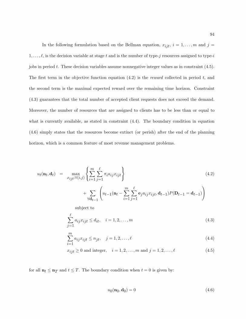
94
In the following formulation based on the Bellman equation, xijt, i = 1, . . . , m and j =
1, . . . , `, is the decision variable at stage t and is the number of type-j resources assigned to type-i
jobs in period t. These decision variables assume nonnegative integer values as in constraint (4.5).
The first term in the objective function equation (4.2) is the reward collected in period t, and
the second term is the maximal expected reward over the remaining time horizon. Constraint
(4.3) guarantees that the total number of accepted client requests does not exceed the demand.
Moreover, the number of resources that are assigned to clients has to be less than or equal to
what is currently available, as stated in constraint (4.4). The boundary condition in equation
(4.6) simply states that the resources become extinct (or perish) after the end of the planning
horizon, which is a common feature of most revenue management problems.
ut(nt,dt) = maxxijt:∀(i,j)
m∑
i=1
∑
j=1πiaijxijt
(4.2)
+∑
∀dt−1
ut−1(nt −
m∑
i=1
∑
j=1ejaijxijt,dt−1)P (Dt−1 = dt−1)
subject to
∑
j=1aijxijt ≤ dit, i = 1, 2, . . . , m (4.3)
m∑
i=1aijxijt ≤ njt, j = 1, 2, . . . , ` (4.4)
xijt ≥ 0 and integer, i = 1, 2, . . . , m and j = 1, 2, . . . , ` (4.5)
for all nt ≤ nT and t ≤ T . The boundary condition when t = 0 is given by:
u0(n0,d0) = 0 (4.6)

95
The optimal solution to stochastic dynamic programs can be found using the standard
backward induction method. However, the applicability of dynamic programming to many prac-
tical problems is limited by the enormous size of the state spaces, better known as the curse
of dimensionality (Bellman 1961). For such problems, Bertsekas & Tsitsiklis (1998) propose a
class of approximate dynamic programming formulations, which they refer to as neuro-dynamic
programming. When making a decision at the current stage, they use an approximation of the
reward function instead of the optimal in the Bellman equation. The way this approximate re-
ward function is constructed is a key issue in their approach to the problem: the rollout heuristic
simulates the system under a selected policy, called the base policy, beginning from the next stage,
and applies the policy for all possible states of the problem. Then, the decision which yields to
the state with the maximum heuristic reward is selected. Although this is a straightforward tech-
nique to implement, it significantly improves on the performance of the base policy (Bertsekas,
Tsitsiklis & Wu 1997, Bertsekas & Castanon 1999). However, Bertsekas (1997) also points out
that the performance of the heuristic might be particularly sensitive to simulation and approxi-
mation error, and he presents a more robust technique, based on estimating differential reward
functions rather than absolute values. As an alternative way of determining approximate reward
functions, without simulation, Bertsekas & Tsitsiklis (1998) suggest using certainty equivalence
approximations, in which the reward of the next stage is computed by simply assuming fixed
values for the problem unknowns. Variations of rollout heuristic have been successfully applied
to many dynamic programming areas, varying from Markov games (Chang & Marcus 2001) to
scheduling of straight-line code compilers (McGovern & Moss 1998).
A class of problems similar to our revenue management problem is the dynamic and stochas-
tic knapsack problem (DSKP). Kleywegt & Papastavrou (1998) define DSKP as the allocation

96
problem of limited resources to competing items with random arrival times, resource require-
ments (size), and rewards, which are usually unknown before arrival. The acceptance decisions
are made sequentially as items arrive. If an item is accepted, the required amount of the resource
is allocated. Note that, the knapsack is a single flexible resource that can be used for all arriving
items. Kleywegt & Papastavrou (1998) study both finite and infinite horizon cases of the prob-
lem, assuming equal item sizes. They show that a threshold-type policy based on item rewards is
optimal for both cases. They also derive structural characteristics, such as concavity and mono-
tonicity, of the optimal value function and the optimal acceptance threshold, which intuitively
becomes more lenient with time. Further, they obtain closed-form solutions for the special case of
exponentially distributed random rewards. Kleywegt, Papastavrou & Rajagopalan (1996) study
the finite horizon version of the DSKP but consider several cases reflecting different operating
conditions : (1) random rewards and equal sizes, (2) random sizes and equal rewards, and (3)
random rewards and sizes. For the case where the item sizes and rewards are both random, they
demonstrate that the optimal decision rule might display the intuitive the anticipated character-
istics unless a consistency condition for the distribution of item sizes given rewards is satisfied.
Verweij et al. (2001) extend these results to the infinite horizon DSKP and focus particularly on
the random sized items. They show that many of the optimality results established in Kleywegt
& Papastavrou (1998) still hold, but some of the intuitive features of the optimal solutions fail to
generalize. Hence, they identify the conditions under which these features continue to hold.
4.4 Special Cases and Properties
When we defined the online assignment of flexible resources problem, independence across
different time periods was the only assumption we made about the demands for the jobs. Hence,
97
we did not assume any particular probability distribution function in the dynamic programming
formulation of the problem given in section (4.3.3). We now consider some special cases of our
problem with the intention of getting insight on the structure of the optimal policy. By making a
number of simplifying assumptions about the demand distributions and restricting our attention
to smaller sized problems, we believe that some important characteristics of the optimal policy,
otherwise almost impossible to detect with the general setup of the problem, would be observed.
Our ultimate goal from the analysis of these special cases is to gain sufficient intuition to develop
heuristics that would capture the behavior of the optimal policy.
4.4.1 A Model for Two Types of Jobs and Three Types of Resources with Multi-
nomially Distributed Demand
We consider a T period, finite horizon discrete-time system with two types of jobs, 1 and
2, and three types of resources, 1, 2 and 3. Type-1 and type-2 resources are special-purpose and
can be assigned to type-1 and type-2 jobs, respectively. On the other hand, type-3 resource is
a flexible resource. In each period, a type-i job is requested with probability pi, where pi is the
probability that the requested job is of type-i, i = 1, 2. We assume that p1 + p2 ≤ 1. Therefore,
in each period there is a probability of 1 − p1 − p2 with which no jobs are requested at all. In
the dynamic programming formulation of this simple case, the state of the system at any given
time is defined by the number of available resources nt = (n1t, n2t, n3t) and the demand in the
period, ei, i = 1, 2. Then let ut(n1t, n2t, n3t; ej) be the maximum expected revenue attainable,
given that the number of resources are (n1t, n2t, n3t) and a type-i job is requested in period t,
i = 1, 2. The Bellman recursive equations of ut(n1t, n2t, n3t; ei) are given in (4.2)-(4.6). Similarly,
let ut(n1t, n2t, n3t) be the maximum expected profit attainable in period t, given that the number
of resources are (n1t, n2t, n3t), before the arrival of a request, if any. Therefore, we can express
98
ut(n1t, n2t, n3t) as follows:
ut(n1t, n2t, n3t) = p1ut(n1t, n2t, n3t; e1)
+ p2ut(n1t, n2t, n3t; e2) (4.7)
+ (1− p1 − p2)ut−1(n1t, n2t, n3t)
Based on the next theorem, there exists an optimal online policy which does not assign a
type-3 resource to a type-i job unless all type-i resources, i = 1, 2, are exhausted.
Theorem 13. For each period t,
1. there exists an optimal policy that assigns a type-1 demand to a type-1 (special purpose)
resource if n1t > 0, and to a type-3 (flexible) resource when n1t = 0 and n3t > 0.
2. there exists an optimal policy that assigns a type-2 demand to a type-2 (special purpose)
resource if n2t > 0.
Proof. We prove statements (1) and (2) by induction on t. These statements are trivially true
for t = 1. We show both statements hold for t, based on the hypothesis that they are valid for
periods 1, 2, . . . , t− 1.
First, we prove that a type-i job should never be rejected when nit > 0, i = 1, 2. Suppose
in period t the optimal policy, say φ∗, rejects a type-i job when nit > 0. From next period onward,
φ∗ will assign type-i resources to type-i jobs whenever possible, by our hypothesis. Let σ < t be
the (random) time when policy φ∗ utilizes its last unit of type-i resource for a type-i job (recall
that time is ordered backwards). We let σ = 0 if this event never happens. Now, let φ′ be another
policy which takes the same actions as φ∗ in each period except in periods t and σ. In period t,
policy φ′ assigns a type-i resource to the type-i job. Since φ′ takes the same actions as that of φ∗
99
during t − 1, . . . , σ + 1, at time σ we have niσ = 0 under φ′. Suppose that φ′ rejects the type-i
demand in period σ. The states of the systems under the two policies are identical after σ. Since
the decisions under the two policies are identical except for the type-i jobs requested in periods
t and σ, the difference under the two policies is equal to the difference between the two rewards
the system receives in periods t and σ. If σ > 0, then φ∗ receives 0 in period t and πi in period σ,
whereas φ′ receives πi in period t and 0 in period σ; hence the two policies perform equally well.
If σ = 0 (the planning horizon ends), then φ∗ and φ′ receive 0 and πi in period t, respectively, so
the performance of φ′ is strictly better than that of φ∗.
Next we show that in period t, a type-3 resource (the flexible resource) should not be
assigned to a type-i job when nit > 0. Without loss of generality let i = 2 (another case can be
proved similarly). Suppose that the optimal policy φ∗ assigns a type-3 resource to a type-2 job
in period t. From next period onward, however, the optimal policy will assign type-i resources to
type-i jobs whenever possible, by our hypothesis. Let σ < t correspond to the time that policy φ∗
utilizes its last unit of type-2 resource for a type-2 job. Let σ = 0 if this event never happens. Also
let γ < 0 be the first time that φ∗ rejects a type 1 job because its type 1 and type 3 resources are
exhausted (by hypothesis, a type 1 job will be accepted whenever possible after time t). Again,
let γ = 0 if this event never occurs. Now, consider another policy φ′ which takes the following
actions: φ′ assigns a type-2 resource to the type-2 job in period t, and takes the same actions as
that of the optimal policy in periods t−1, . . . , min{σ, γ}+1. If σ > γ ≥ 0, let φ′ assign the type-2
demand to the type-3 resource at time σ. The numbers of resources under the two policies are
identical after σ. It is clear that the rewards under the two policies are identical. If 0 < σ < γ,
then let φ′ assign the type-1 job to its last type-3 resources at time γ and rejects the type-2 job
at time σ > 0 (recall at time σ policy φ∗ will utilize its last type 2 resource and policy φ′ has

100
exhausted type-2 resources). Then it can be seen that the extra revenue earned by policy φ′ is
π1 − π2 ≥ 0. If 0 = σ < γ, then policy φ′ accepts one more type-1 job and receives extra revenue
π1. Finally, if 0 = σ = γ, then the revenues received under both policies are identical. Therefore,
the performance of φ′ is better than that of φ∗.
Finally, we show that a type-1 job should use a type-3 resource in period t when n1t = 0
and n3t > 0. Suppose that the optimal policy φ∗ rejects a type-1 job in period t when n1t = 0
and n3t > 0. From next period onward, the optimal policy will assign type-3 resources to type-1
jobs whenever possible, by our hypothesis. Let γ < t be the time when policy φ∗ utilizes its last
unit of type-3 resource either for a type-1 or a type-2 job. We let γ = 0 when this never happens.
Consider another policy φ′ which takes the same actions as φ∗ in each period except in periods t
and γ. In period t, policy φ′ assigns a type-3 resource to the type-1 job. Since φ′ takes the same
actions as that of φ∗ during t− 1, . . . , γ + 1, at time γ we have n3γ = 0 under φ′. Suppose that
φ′ rejects the type-i demand in period σ. The states of the systems under the two policies are
identical after γ. Since the decisions under the two policies are identical except for the type-1
job in period t and the type-i job in period γ, the difference under the two policies is equal to
the difference between the two rewards the system receives in periods t and γ. If γ > 0, then φ∗
receives 0 in period t and πi in period γ, whereas φ′ receives π1 in period t and 0 in period γ.
Then the system under φ′ earns π1 − πi ≥ 0 more than the one under φ∗. If γ = 0, then φ∗ and
φ′ receive 0 and π1 in period t, respectively, so the performance of φ′ is strictly better than that
of φ∗. 2

101
In order to simplify our notation, we drop the time index t from the state variables in our
formulations. The Bellman equations can be written as
ut(n1, n2, n3; e1) =
π1 + ut−1(n1 − 1, n2, n3) if n1 > 0
π1 + ut−1(n1, n2, n3 − 1) if n1 = 0, n3 > 0
ut−1(n1, n2, n3) if n1 = 0, n3 = 0
(4.8)
and
ut(n1, n2, n3; e2) =
π2 + ut−1(n1, n2 − 1, n3) if n2 > 0
max{π2 + ut−1(n1, n2, n3 − 1), ut−1(n1, n2, n3)} if n2 = 0, n3 > 0
ut−1(n1, n2, n3) if n2 = 0, n3 = 0
(4.9)
with the boundary condition u0(n1, n2, n3; ei) = 0 for i = 1, 2.
We define
∆t(n1, n3) = ut(n1, 0, n3 + 1)− ut(n1, 0, n3) (4.10)
and
∆2t (n1, n3) = ut(n1, 0, n3 + 1; e2)− ut(n− 1, 0, n3; e2). (4.11)
From equation (4.9), we see that a type-3 resource is assigned to a type-2 job if and only if
π2 + ut−1(n1, 0, n3 − 1) ≥ ut−1(n1, 0, n3), or, equivalently, π2 ≥ ∆t−1(n1, n3 − 1). Therefore,
the optimal online policy accepts the request for the type-2 job when n2 = 0 and n3 > 0, only if
the corresponding revenue exceeds the opportunity cost of the flexible resource.
Next we develop some structural properties of the cost functions. Based on these properties,
we identify the structure of the optimal online policy. First, it is easy to show that ut(n1, n2, n3; ei)
102
and ut(n1, n2, n3) are increasing in nj , j = 1, 2, 3, and decreasing in t. The next proposition
summarizes the second order properties of cost functions ut(n1, 0, n3; e2) and ut(n1, 0, n3). Recall
that a function f(x, y) is said to be supermodular (submodular) if
f(x, y) + f(x′, y′) ≥ (≤)f(x′, y) + f(x, y′), x ≤ x′, y ≤ y′.
Proposition 14. 1. ut(n1, 0, n3; e2) and ut(n1, 0, n3) are supermodular functions of n1 and
n3, for any t = 1, 2, . . . , T . In other words, ∆2t (n1, n3) and ∆(n1, n3) are nonincreasing in
n1, for any n3 ≥ 0 and t = 1, 2, . . . , T .
2. ut(n1, 0, n3; e2) and ut(n1, 0, n3) are concave functions of n3 for any n1 ≥ 0 and t =
1, 2, . . . , T . In other words, ∆2t (n1, n3) and ∆(n1, n3) are nonincreasing in n3 for any
n1 ≥ 0 and t = 1, 2, . . . , T .
3. ut(n1, 0, n3) is a submodular function of t and n3 for any n1 ≥ 0. In other words, ∆t(n1, n3)
is nondecreasing in t for any n1 ≥ 0 and n3 ≥ 0.
4. (a) ∆2t (n1, n3) ≤ ∆2
t (n1 + 1, n3 − 1) for t = 1, . . . , T and n3 > 0.
(b) ∆t(n1, n3) ≤ ∆t(n1 + 1, n3 − 1) for t = 1, . . . , T and n3 > 0.
Proof. The proof of this proposition is given in the Appendix.
Proposition 14 states that the opportunity cost ∆(n1, n3) becomes smaller as the numbers
of special-purpose and flexible resources become larger and as t becomes smaller (i.e., towards
the end of the planning horizon). In addition, it is more valuable to have an extra unit of flexible
resources than to have an extra unit of special purpose resources.
Based on these preliminary results, we propose the following theorem for the optimal online
policy.
103
Theorem 15. Let (n1, 0, n3; e2) be the state of the system in period t, t = 1, 2, . . . , T .
1. There exists a nonincreasing function Ft(n1) such that a type-2 demand is accepted and
assigned to a type-3 resource if and only if n3 ≥ Ft(n1).
2. If it is optimal to allocate a type-3 resource to the type-2 demand in state (n1, 0, n3) in
period t, then it is also optimal to do the same in state (n1, 0, n3) in period t− 1.
3. If it is optimal to allocate a type-3 resource to the type-2 demand in state (n1 + 1, 0, n3− 1)
in period t, then it is also optimal to do the same in state (n1, 0, n3) in period t.
Proof. For part (1) of the theorem, we define
Ft(n1) = min{n3 : ∆t−1(n1, n3 − 1) ≤ π2} (4.12)
From Proposition 14 (1) and (2), we can conclude Ft(n1) is nonincreasing in n1. Theorem 13 (1)
and (2) also implies for any k ≥ 1,
∆t−1(n1, n3) ≤ π2 =⇒ ∆t−1(n1 + k, n3) ≤ π2, (4.13)
∆t−1(n1, n3) ≤ π2 =⇒ ∆t−1(n1, n3 + k) ≤ π2. (4.14)
In other words, if a type-3 resource is allocated to a type-2 job in state (n1, 0, n3) in period t, then
it should also allocate a type-3 resource in states (n1 + k, 0, n3) and (n1, 0, n3 + k), respectively,
in period t. Clearly, Ft(n1) serves as the threshold such that a type-2 demand is accepted in state
(n1, 0, n3) if and only if n3 ≥ Ft(n1).
Now, Proposition 14 (3) implies that Ft(n1) is an increasing function of t, which implies
part (2) of the theorem.

104
Finally, by Proposition 14 (3),
π2 ≥ ∆t(n1 + 1, n3 − 1) =⇒ π2 ≥ ∆t(n1, n3),
which implies part (3) of the theorem. 2
For a specific time period t, the nonincreasing function Ft(n1) determines the threshold
that the number of type-3 resources should exceed in order for them to be assigned to a type-2
job in state (n1, 0, n3; e2). Figure 4.1 illustrates this threshold-type online policy. Only when
(n1, n3) falls into the acceptance region, the request for the type-2 job is accepted in period t.
n3
n1
Acceptance
Region
Rejection
Region
Ft(n1)
1
1n 2
1n
1
3n
2
3n
job2eReject typ:)n,n( 1
3
1
1
job2eAccept typ:)n,n( 2
3
2
1
Fig. 4.1. Threshold-type optimal policy: Ft(n1) a nonincreasing function of n1
In part (3) of Proposition 14, we proved that ∆t(n1, n3) is a nondecreasing function of t
for any n1 and n3. Therefore, Ft(n1) is also a nondecreasing function of t for a given n1, from the
definition in (4.12). In other words, the optimal policy becomes more lenient towards accepting
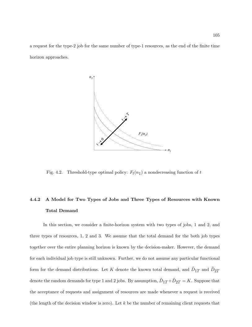
105
a request for the type-2 job for the same number of type-1 resources, as the end of the finite time
horizon approaches.
n3
n1
Ft(n1)
t
T
t
0
Fig. 4.2. Threshold-type optimal policy: Ft(n1) a nondecreasing function of t
4.4.2 A Model for Two Types of Jobs and Three Types of Resources with Known
Total Demand
In this section, we consider a finite-horizon system with two types of jobs, 1 and 2, and
three types of resources, 1, 2 and 3. We assume that the total demand for the both job types
together over the entire planning horizon is known by the decision-maker. However, the demand
for each individual job type is still unknown. Further, we do not assume any particular functional
form for the demand distributions. Let K denote the known total demand, and D1T and D2T
denote the random demands for type 1 and 2 jobs. By assumption, D1T +D2T = K. Suppose that
the acceptance of requests and assignment of resources are made whenever a request is received
(the length of the decision window is zero). Let k be the number of remaining client requests that

106
is yet to arrive, including the job that has just arrived, k = 1, 2, . . . , K. Each request represents a
stage in the process and hence k indexes the stages. Assume that k = K corresponds to the first
arrival and k = 1 to the last arrival of client requests during the planning horizon. The number
of available type-j resources at stage k is denoted as njk.
We propose the following online decision rule for whether or not to accept the client’s
request for a job and which resource to assign if the request is accepted:
Algorithm 16. Online decision rule for Case 2:
1. If the current request is for a type-1 job:
• accept if n1k + n3k > 0; otherwise reject;
• if accepted, assign a type-1 resource if n1k > 0, or a type-3 resource if n1k = 0.
2. If the current request is for a type-2 job:
• accept if n2k > 0 or n1k + n3k ≥ k; otherwise reject;
• if accepted, assign a type-2 resource if n2k > 0, else assign a type-3 resource.
As a type-1 job is more profitable than a type-2 job, the optimal online policy always accepts
requests for type-1 job, if possible. Therefore, our decision rule is also designed to accept a
client’s request for a type-1 job, as long as there is at least one resource that can process it, i.e.
n1k + n3k > 0. On the other hand, the policy is more selective in accepting requests for type-2
jobs. It accepts a request for a type-2 job if there exists a special-purpose resource for that job.
Otherwise, a threshold criteria, k ≤ n1k +n3k, should be satisfied so that a request for the type-2
job is accepted. Notice that k − 1 is the maximum number of remaining requests for the type-1
jobs. If there are enough resources for all those requests, rejecting the current request for a type-2
107
job will lead to an unused flexible resource at the end. We refer to k ≤ n1k + n3k condition as
the 2-flex assignment condition. Next, we prove that the our decision policy is equivalent to the
optimal online policy for this problem. However, it is useful to state the following proposition
first.
Proposition 17. If at some stage k, the 2-flex assignment condition is satisfied, then this con-
dition must hold at all subsequent stages.
Proof. Suppose the 2-flex assignment condition is satisfied at some stage k. Then,
k ≤ n1k + n3k
Since we assign no more than one resource at this stage, we have:
k − 1 ≤ n1k + n3k − 1
≤ n1(k−1) + n3(k−1)
Consequently, the 2-flex condition is also satisfied at stage k-1. 2.
Proposition 17 implies that, once we begin assigning flexible resources to type-2 jobs, we
continue accepting all subsequent type-2 jobs, until flexible resources are exhausted. Let k∗ be
the first stage at which the 2-flex assignment condition is satisfied. Then,
k∗ = max{k = 1, . . . , K : k ≤ n1k + n3k} (4.15)
We define k∗ = 0 if the 2-flex condition is never satisfied at any stage k = 1, . . . , K. Notice that
k∗ is a random variable which may take values 0, 1, . . . , K, depending on the problem instance

108
(i.e., the available resources, total demand K, realization of the demands for type-1 and type-2
jobs, and the sequence of jobs).
If k∗ = K, then whenever a demand for type-2 job arrives, our decision rule in Algorithm
16 accepts it if n2k + n3k > 0. Conversely, if k∗ = 0, the decision rule accepts no more than
n2K type-2 jobs; furthermore, no type-1 and type-3 resources are left unused at the end. This
last observation follows by noting that, if k∗ = 0, then the 2-flex assignment condition was not
satisfied at stage k = 1, i.e. n11 + n31 < 1; consequently, n11 + n31 = 0.
In the following theorem, we compare the performance of the online decision rule in Algo-
rithm 16 with that of the optimal solution.
Theorem 18. For any set of resources, realization of demands D1 and D2 (with D1 +D2 = K),
and sequence of arrivals of these demands, the Algorithm 16 solution has the same total revenue
as the optimal solution.
Proof. First note that, in assigning resources to the accepted jobs, Algorithm 16 gives priority to
the corresponding special purpose resources over the flexible resource, which is optimal. Hence, if
we can show that the algorithm accepts the same number of type-1 and type-2 jobs as the optimal
solution, then the two solutions must also have the same total revenues.
In our proof of this theorem, we consider the following three cases:
Case 1 (k∗ = 0): As we noted earlier, Algorithm 16 exhausts all of the type-1 and type-3 re-
sources, and uses these resources exclusively for type-1 jobs. Clearly, the optimal solution
can do no better.
Case 2 (k∗ = K): By Proposition 17, the 2-flex assignment condition will be satisfied for all k =
1, . . . , K. Therefore, no requests for the type-2 jobs will be rejected as long as n2k+n3k > 0,
109
and all type-1 jobs will be accepted under Algorithm 16. Clearly, the optimal solution can
do no better.
Case 3 (0 < k∗ < K): By definition, we have
k∗ = n1k∗ + n3k∗ for 0 < k∗ < K (4.16)
This implies that, under Algorithm 16, no request for a type-1 job will be rejected either
before or after k∗. Since the optimal solution will accept as many type-1 jobs as possible,
the number of type-1 jobs accepted by the two solutions must be identical. Next, we show
that the two solutions also accept the same number of type-2 jobs.
First, if n1k∗ = 0, all of the n3k∗ type-3 resources will be exhausted by the type-1 and
type-2 jobs. Since the number of type-1 jobs accepted by the two solutions is identical, the
number of type-2 jobs accepted by the two solutions should also be the same.
Next, assume n1k∗ > 0, which implies that no type-3 resource has been utilized by either
job types. Hence, n3k∗ = n3K . If the demand for type-1 jobs after k∗ is greater than or
equal to n1k∗ , then all n1k∗ and n3k∗ resources will be exhausted by type-1 and type 2
jobs under Algorithm 16. Based on our previous argument, this means that the number of
type-2 jobs accepted by our decision rule is the same as the one under the optimal policy.
If the demand for type-1 jobs after k∗ is less than n1k∗ , all n3K type-3 resources will be
allocated to type-2 jobs, with no request for a type-1 job being ever rejected. Clearly, the
optimal solution cannot accept more type-2 tasks than Algorithm 16.

110
We see that in all three cases, our online decision rule accepts the same number of jobs as the
optimal solution, and therefore generates an equal amount of revenue. Hence, Algorithm 16
optimally solves the problem. 2
Algorithm 16 is an optimal online policy and is independent of the distributions of the job
demands as long as the total number of arrivals is known in advance. This optimal policy can
be classified as a threshold-type policy, since the jobs are accepted if a threshold criteria for the
resources, based on future arrivals of the jobs, is satisfied. Notice that the structure of Algorithm
16 is the same as the optimal policy prescribed in Theorem 4.12. Remember that, according to
this theorem, if n2k = 0 and n3k > 0, there exists a nonincreasing function F (n1k) such that
a type-2 job is accepted and a type-3 resources is assigned to it if and only if n3k ≥ F (n1k).
On the other hand, our decision rule assigns a type-3 resource to a type-2 job if n1k + n3k ≥ k.
Therefore, F (n1k) for Algorithm 16 is equal to k−n1k, which clearly is a nonincreasing function
of n1k.
4.4.3 A Two Period Model for Two Types of Jobs and Three Types of Resources
In this section, we consider a two period model with two types of jobs, 1 and 2, and three
types of resources, 1, 2 and 3. Initially, we assume that only type-1 jobs arrive in the second
period. We adopt a static allocation policy based on the newsboy model, that limits the number
of flexible resources to be used for type-2 jobs. Suppose that the number of type-2 resources is
equal to zero, without loss of generality. Define Q3 as the booking limit on type-3 resources for
type-2 jobs. Let F1(D1) be the cdf of the random variable D1, and F2(D2) be the pdf of D2. We
denote the pdf’s by f1(D1) and f2(D2), respectively. Given state (n1, 0, n3; 0, d2), we can write

111
the reward function at t = 2 as:
u2(n1, 0, n3; 0, d2) = maxQ3≤min(d2,n3)
{π2Q3 + E[u1(n1, 0, n3 −Q3; D1, 0]}
= maxQ3≤min(d2,n3)
{π2Q3 + π1E[min(n1, D1)]
+ π1E[min(n3 −Q3, (D1 − n1)+]}
= maxQ3≤min(d2,n3)
{π2Q3 + π1
∫ n1
0(1− F1(x1))dx1
+ π1
∫ n3−Q3
0(1− F1(x1 + n1))dx1}
The function
f(n1, n3, Q3) = π2Q3 + π1
∫ n1
0(1− F1(x))dx1 + π1
∫ n3−Q3
0(1− F1(x + n1))dx1
is concave in Q3 for Q3 ≤ n3. Taking the partial of f(n1, n3, Q3) with respect to Q3 yields
∂f(n1, n3, Q3)∂Q3
= π2 − π1(1− F1(n1 + n3 −Q3))
Let Q∗ satisfy
F1(Q∗) =π1 − π2
π1, (4.17)
where Q∗ is understood as the optimal total number of type-1 and type-3 resources needed for the
future arrivals of type-1 jobs. From the above expressions, we obtain Q∗3, the number of type-3

112
resources that can be used to satisfy the demand for type-2 jobs, must satisfy
Q∗3 =
n3 if Q∗ ≤ n1
n1 + n3 −Q∗ if n1 < Q∗ ≤ n1 + n3
0 if Q∗ > n1 + n3
Therefore, we can use as many as Q∗3 type-3 resources to meet the the current demand for type-2
jobs.
The result in equation (4.17) is along the same lines with that of the traditional newsboy
problem. In effect, we solve the newsboy problem that determines the number of flexible resources
to be reserved for the more profitable jobs. Therefore, Q∗ is a function of the number of available
resources, revenues and the probability distribution of D1, but is independent of the probability
distribution of D2. Suppose that we fail to satisfy a request for a type-1 job because we do not
reserve enough type-3 resources. Then, we would not be able to collect the revenue from the
type-1 job, but still meet the demand for a type-2 job. On the other hand, if we reserve more
type-3 resources than what is indeed needed for type-1 jobs, we would loose the revenue from a
type-2 job. Hence, π1 − π2 is the underage cost and π2 is the overage cost of the type-3 resource
in this model. After rearranging the terms in equation (4.17), we can write:
F1(Q∗) =π1 − π2
π1=⇒ P{D1 > Q∗} =
π2π1
(4.18)
4.4.4 Network Flow Models
In Section 4.3.3, we modelled the revenue management problem as a stochastic dynamic
program, which provides the optimal policy for the acceptance of jobs and assignment of resources.

113
Remember that, these decisions are made at the end of each period after the demand is received.
Therefore, the decision-maker has to consider the future demand for jobs, availability of resources,
revenues from different jobs, among many other things.
Suppose that the decision-maker is granted full information about the aggregate future
demand of every job type over the remaining t periods. Consequently, the decision-maker faces a
deterministic, single period problem, where the acceptance and assignment decisions are deferred
to the end of the planning horizon. This problem can be formulated as a network flow model,
which we refer to as the omniscient model, as follows:
ut(nt, dt) = maxm∑
i=1
∑
j=1πiaijxij
subject to
Demand constraints :∑
j=1aijxij ≤ dit, i = 1, . . . , m (4.19)
Supply constraints :m∑
i=1aijxij ≤ njt, j = 1, . . . , `
xij ≥ 0 and integer, i = 1, . . . ,m, j = 1, . . . , `
The above integer program maximizes the total revenue in the remaining t periods given the
realized demand dt, and the set of currently available resources nt. The decision variable xij ,
i = 1, . . . , m, j = 1, . . . , `, denotes the total number of type-j resources allocated to type-i jobs,
and assumes nonnegative integer values.
Note that the formulation in (4.19) determines the optimal policy for a particular demand
scenario. Since the aggregate demand for each job type in the remaining t periods is a random
variable, the optimal revenue is also a random variable, dependant on Dt. The expected value of
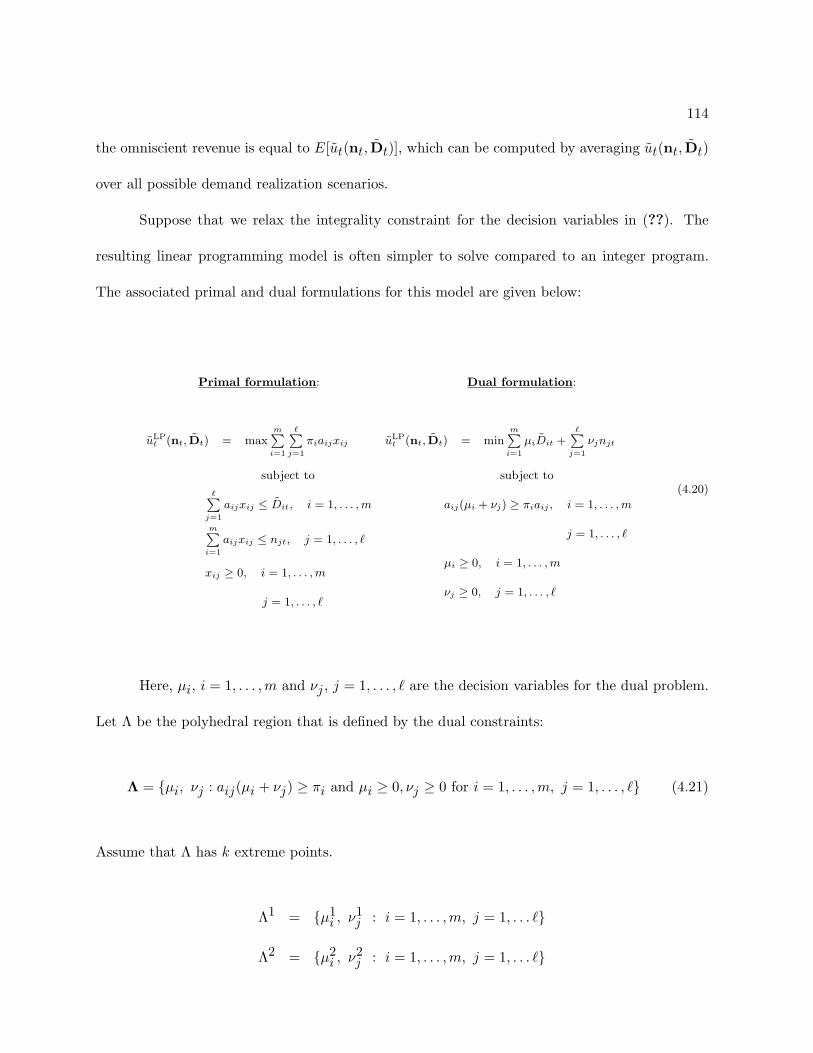
114
the omniscient revenue is equal to E[ut(nt, Dt)], which can be computed by averaging ut(nt, Dt)
over all possible demand realization scenarios.
Suppose that we relax the integrality constraint for the decision variables in (??). The
resulting linear programming model is often simpler to solve compared to an integer program.
The associated primal and dual formulations for this model are given below:
Primal formulation: Dual formulation:
uLPt (nt, Dt) = max
m∑i=1
∑j=1
πiaijxij
subject to
∑j=1
aijxij ≤ Dit, i = 1, . . . , m
m∑i=1
aijxij ≤ njt, j = 1, . . . , `
xij ≥ 0, i = 1, . . . , m
j = 1, . . . , `
uLPt (nt, Dt) = min
m∑i=1
µiDit +∑j=1
νjnjt
subject to
aij(µi + νj) ≥ πiaij , i = 1, . . . , m
j = 1, . . . , `
µi ≥ 0, i = 1, . . . , m
νj ≥ 0, j = 1, . . . , `
(4.20)
Here, µi, i = 1, . . . , m and νj , j = 1, . . . , ` are the decision variables for the dual problem.
Let Λ be the polyhedral region that is defined by the dual constraints:
Λ = {µi, νj : aij(µi + νj) ≥ πi and µi ≥ 0, νj ≥ 0 for i = 1, . . . ,m, j = 1, . . . , `} (4.21)
Assume that Λ has k extreme points.
Λ1 = {µ1i , ν1
j : i = 1, . . . ,m, j = 1, . . . `}
Λ2 = {µ2i , ν2
j : i = 1, . . . ,m, j = 1, . . . `}
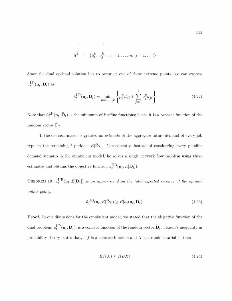
115
......
Λk = {µki , νk
j : i = 1, . . . ,m, j = 1, . . . `}
Since the dual optimal solution has to occur at one of these extreme points, we can express
uLPt (nt, Dt) as:
uLPt (nt, Dt) = min
y=1,...,k
µ
yi Dit +
∑
j=1νyj njt
(4.22)
Note that uLPt (nt, Dt) is the minimum of k affine functions; hence it is a concave function of the
random vector Dt.
If the decision-maker is granted an estimate of the aggregate future demand of every job
type in the remaining t periods, E[Dt]. Consequently, instead of considering every possible
demand scenario in the omniscient model, he solves a single network flow problem using these
estimates and obtains the objective function uUBt (nt, E[Dt]).
Theorem 19. uUBt (nt, E[Dt]) is an upper-bound on the total expected revenue of the optimal
online policy.
uUBt (nt, E[Dt]) ≥ E[ut(nt,Dt)] (4.23)
Proof. In our discussions for the omniscient model, we stated that the objective function of the
dual problem, uLPt (nt, Dt), is a concave function of the random vector Dt. Jensen’s inequality in
probability theory states that, if f is a concave function and X is a random variable, then
Ef(X) ≤ f(EX) (4.24)
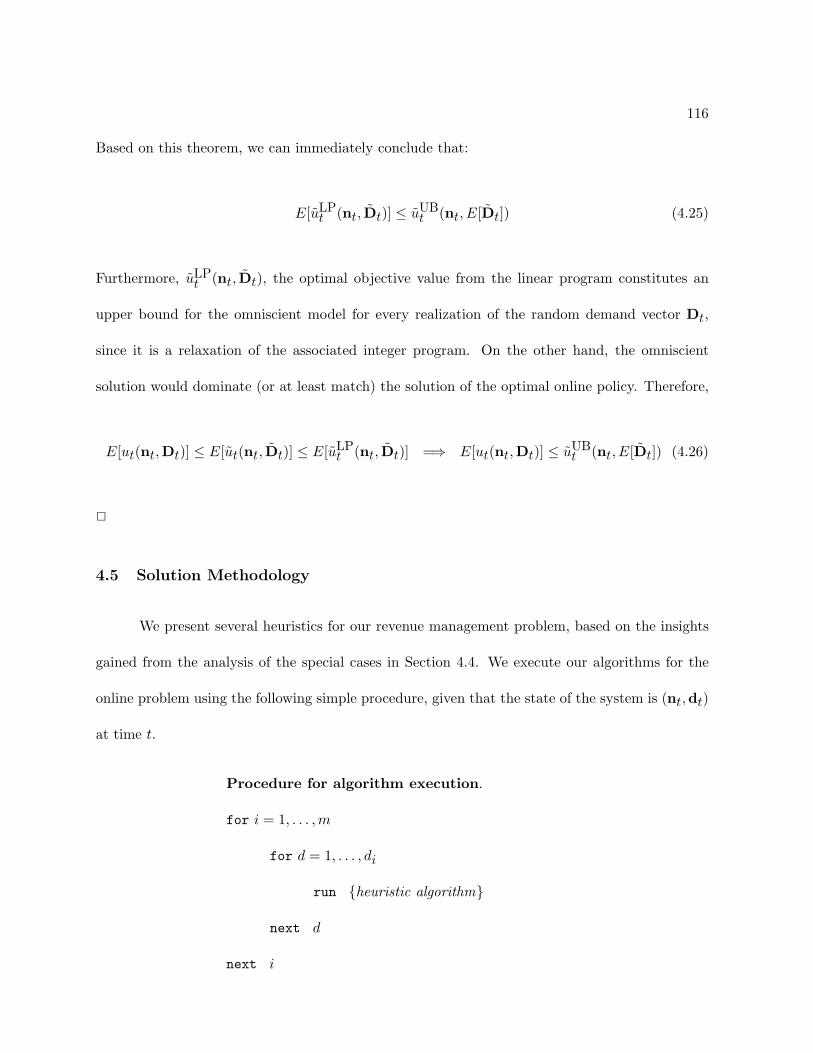
116
Based on this theorem, we can immediately conclude that:
E[uLPt (nt, Dt)] ≤ uUB
t (nt, E[Dt]) (4.25)
Furthermore, uLPt (nt, Dt), the optimal objective value from the linear program constitutes an
upper bound for the omniscient model for every realization of the random demand vector Dt,
since it is a relaxation of the associated integer program. On the other hand, the omniscient
solution would dominate (or at least match) the solution of the optimal online policy. Therefore,
E[ut(nt,Dt)] ≤ E[ut(nt, Dt)] ≤ E[uLPt (nt, Dt)] =⇒ E[ut(nt,Dt)] ≤ uUB
t (nt, E[Dt]) (4.26)
2
4.5 Solution Methodology
We present several heuristics for our revenue management problem, based on the insights
gained from the analysis of the special cases in Section 4.4. We execute our algorithms for the
online problem using the following simple procedure, given that the state of the system is (nt,dt)
at time t.
Procedure for algorithm execution.
for i = 1, . . . , m
for d = 1, . . . , di
run {heuristic algorithm}
next d
next i
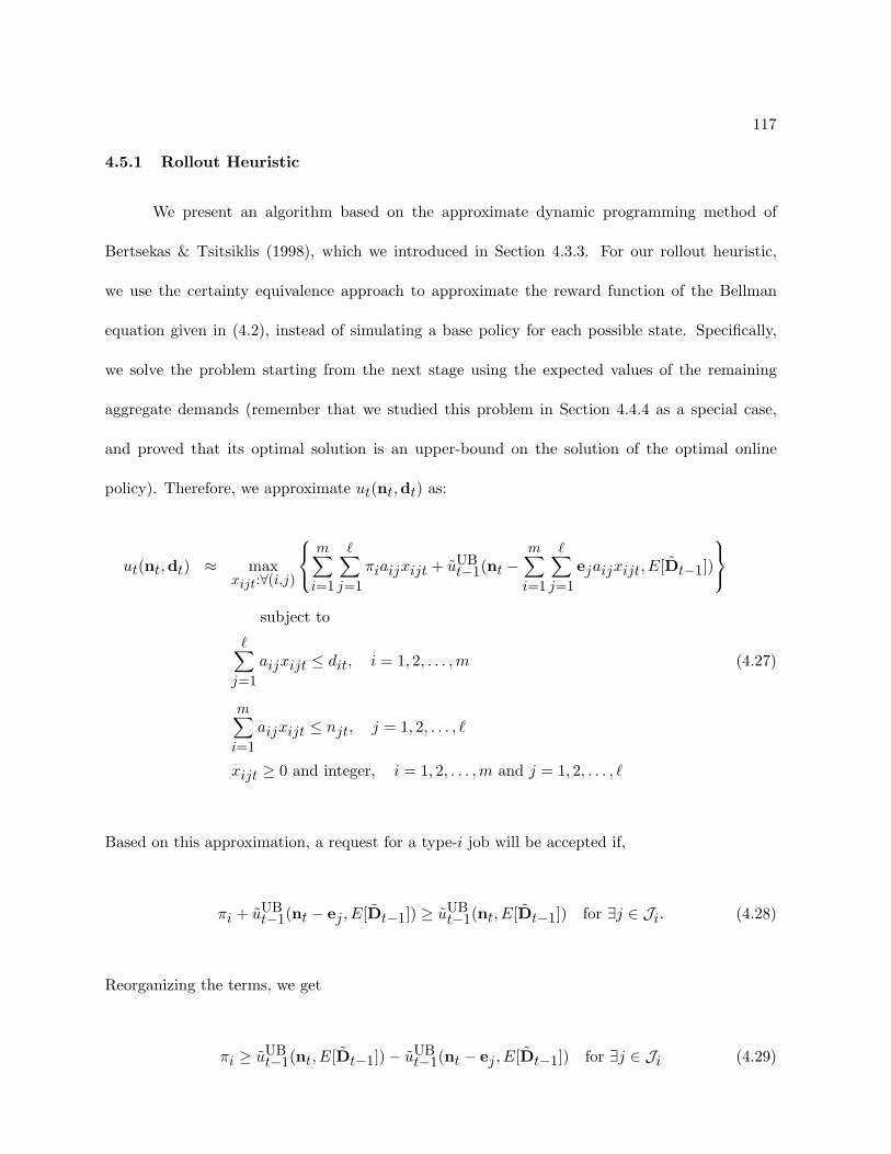
117
4.5.1 Rollout Heuristic
We present an algorithm based on the approximate dynamic programming method of
Bertsekas & Tsitsiklis (1998), which we introduced in Section 4.3.3. For our rollout heuristic,
we use the certainty equivalence approach to approximate the reward function of the Bellman
equation given in (4.2), instead of simulating a base policy for each possible state. Specifically,
we solve the problem starting from the next stage using the expected values of the remaining
aggregate demands (remember that we studied this problem in Section 4.4.4 as a special case,
and proved that its optimal solution is an upper-bound on the solution of the optimal online
policy). Therefore, we approximate ut(nt,dt) as:
ut(nt,dt) ≈ maxxijt:∀(i,j)
m∑
i=1
∑
j=1πiaijxijt + uUB
t−1(nt −m∑
i=1
∑
j=1ejaijxijt, E[Dt−1])
subject to
∑
j=1aijxijt ≤ dit, i = 1, 2, . . . ,m (4.27)
m∑
i=1aijxijt ≤ njt, j = 1, 2, . . . , `
xijt ≥ 0 and integer, i = 1, 2, . . . , m and j = 1, 2, . . . , `
Based on this approximation, a request for a type-i job will be accepted if,
πi + uUBt−1(nt − ej , E[Dt−1]) ≥ uUB
t−1(nt, E[Dt−1]) for ∃j ∈ Ji. (4.28)
Reorganizing the terms, we get
πi ≥ uUBt−1(nt, E[Dt−1])− uUB
t−1(nt − ej , E[Dt−1]) for ∃j ∈ Ji (4.29)

118
Notice that the opportunity cost given by uUBt−1(nt, E[Dt−1]) − uUB
t−1(nt − ej , E[Dt−1]) is the
change in objective function of (??) for a unit change in the value of njt, which is the definition
of the shadow price associated with the supply constraint of the type-j resources. Let us denote
the shadow price of the type-j resource as νj , j = 1, . . . , `. Our rollout heuristic for the online
assignment problem follows next.
Algorithm 20. Algorithm for the rollout decision policy at time t.
1. Accept a type-i job if and only if its revenue is greater than or equal to the opportunity cost
of assigning an available resource to it, i.e.,
πi ≥ minj∈Ji,njt>0
νj (4.30)
where νj , j = 1, . . . , ` is the shadow price of resource-j in formulation (??).
2. If a type-i job is accepted, then assign a type-j∗ resource, given by:
j∗ = argminj∈Ji,njt>0
νj (4.31)
In the first stage of Algorithm 20, we check whether there exists a resource in set Ji with
a shadow price that at least matches the revenue from the type-i job. If so, we assign the type-j∗
resource that has the minimum opportunity cost, in the second stage.
4.5.2 Threshold Heuristic
In Sections 4.4.1 and 4.4.2, we showed that the optimal online decision rule is a threshold-
type policy for the considered special cases. Specifically, in a simple system with two job types

119
and three resource types, where demand is multinomially distributed in each period, the optimal
online policy accepts a type-2 job if and only if the number of flexible resources exceeds a threshold
value, which is a nonincreasing function of the available special-purpose resources for type-1 jobs,
and a nondecreasing function of remaining time, once the special-purpose resources for type-2
jobs are exhausted. Moreover, if the total demand for the two job types is known by the decision-
maker, the functional form of this policy can be identified. The following algorithm presents a
threshold-type heuristic for the general problem.
Algorithm 21. Algorithm for the threshold-type online decision policy at time t.
1. Accept a type-i job if and only if
(a) either
∑
j∈Ji
njt > 0 where Ji =
j ∈ Ji :
i−1∑
k=1akj = 0
(4.32)
(Here, Ji is the set of resources that can only process type-i or lesser valued job types.)
(b) or the available resources are sufficient to meet the aggregate expected demand for more
valuable jobsi−1∑
k=1
∑
j=1akjnjt ≥
i−1∑
k=1E[Dkt] (4.33)
and there is at least one available resource that can handle the type-i job
∑
j∈Ji
njt > 0. (4.34)

120
2. If a type-i job is accepted, then assign a type-j∗ resource from set Ji, which are defined as
follows:
Ji = argminj∈Ji,njt>0
ϕj (4.35)
(Here Ji is the set of available resources with the smallest level flexibility) and
j∗ = argminj∈Ji
m∑k=1
akjπkE[Dkt]
m∑k=1
akjE[Dkt]
. (4.36)
A brief explanation of Algorithm 21 is in order: the first step of the algorithm verifies
whether the requested type-i job meets either one of the two acceptance criteria. Resource types
in set Ji, as defined in (4.32), can only be assigned to type-i or lesser valued jobs (i.e., jobs with
indices larger than i). Therefore, the algorithm accepts the request immediately if there is at least
one available such resource. Otherwise, the algorithm checks the second acceptance criterion. If
the total number of resources that can be assigned to jobs with higher revenues than that of the
requested type-i job (i.e., jobs with indices larger than i), is less than the aggregate expected
demand for those jobs over the remaining time horizon, the algorithm rejects the current request.
In this situation, the algorithm predicts that these resources have a significant chance of being
used to accept more valuable job. On the other hand, if (4.33) is satisfied, the algorithm ensures
that there is at least one resource that can be assigned to the type-i job, before accepting the
request. The second step of the algorithm determines the type of the resource to be used for the
accepted type-i job. Ji, defined in equation (4.35), is a subset of Ji containing the indices of the
least flexible resources that are currently available. Note that we measure flexibility in terms of
the number of different types of jobs that a particular resource can be assigned to. The algorithm
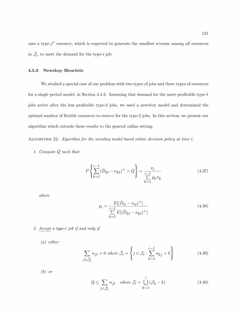
121
uses a type-j∗ resource, which is expected to generate the smallest revenue among all resources
in Ji, to meet the demand for the type-i job.
4.5.3 Newsboy Heuristic
We studied a special case of our problem with two types of jobs and three types of resources
for a single period model, in Section 4.4.3. Assuming that demand for the more profitable type-1
jobs arrive after the less profitable type-2 jobs, we used a newsboy model and determined the
optimal number of flexible resources to reserve for the type-2 jobs. In this section, we present our
algorithm which extends these results to the general online setting.
Algorithm 22. Algorithm for the newsboy model based online decision policy at time t.
1. Compute Q such that:
P
i−1∑
k=1(Dkt − nkt)
+ > Q
=
πii−1∑k=1
pkπk
(4.37)
where
pi =E[(Dit − nit)
+]i−1∑k=1
E[(Dkt − nkt)+](4.38)
2. Accept a type-i job if and only if
(a) either
∑
j∈Ji
njt > 0 where Ji =
j ∈ Ji :
i−1∑
k=1akj = 0
(4.39)
(b) or
Q ≤∑
j∈Ji
njt where Ji =i⋃
k=1(Jk − k) (4.40)
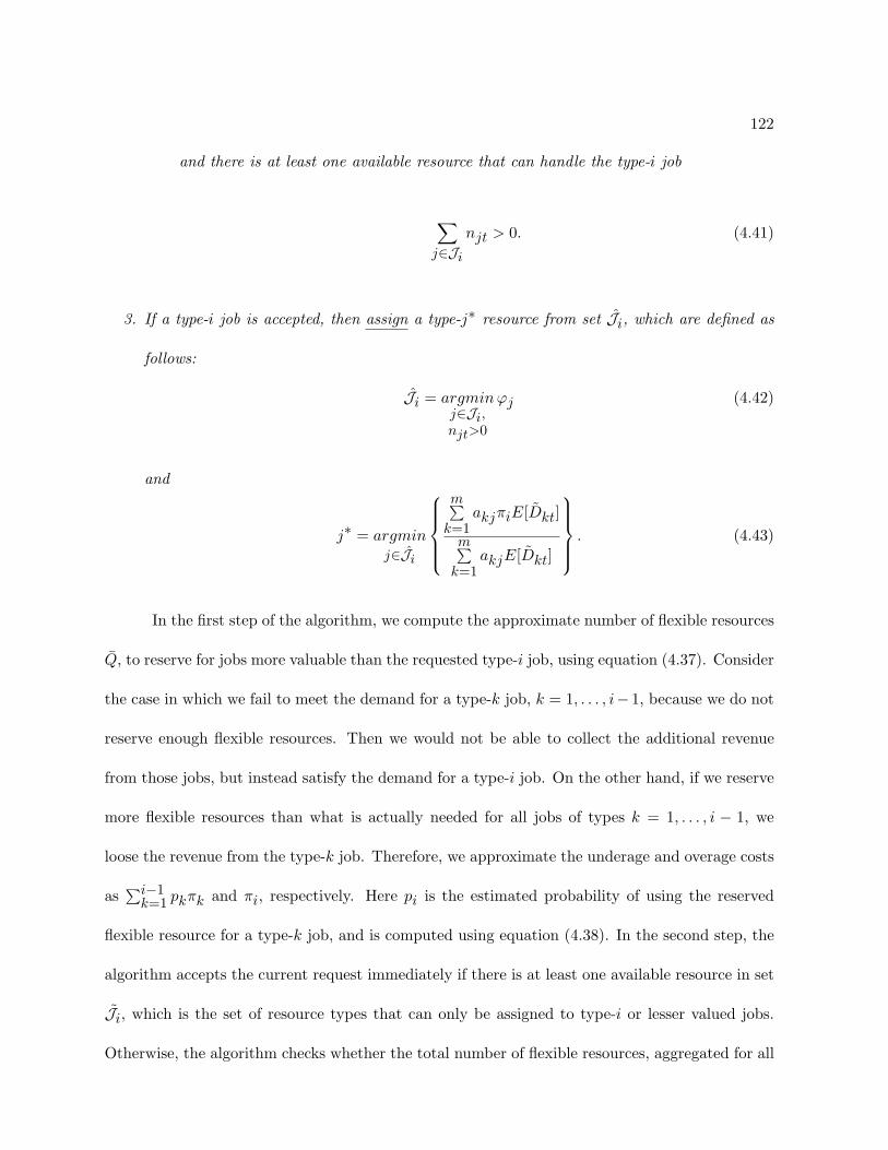
122
and there is at least one available resource that can handle the type-i job
∑
j∈Ji
njt > 0. (4.41)
3. If a type-i job is accepted, then assign a type-j∗ resource from set Ji, which are defined as
follows:
Ji = argminj∈Ji,njt>0
ϕj (4.42)
and
j∗ = argminj∈Ji
m∑k=1
akjπiE[Dkt]
m∑k=1
akjE[Dkt]
. (4.43)
In the first step of the algorithm, we compute the approximate number of flexible resources
Q, to reserve for jobs more valuable than the requested type-i job, using equation (4.37). Consider
the case in which we fail to meet the demand for a type-k job, k = 1, . . . , i− 1, because we do not
reserve enough flexible resources. Then we would not be able to collect the additional revenue
from those jobs, but instead satisfy the demand for a type-i job. On the other hand, if we reserve
more flexible resources than what is actually needed for all jobs of types k = 1, . . . , i − 1, we
loose the revenue from the type-k job. Therefore, we approximate the underage and overage costs
as∑i−1
k=1 pkπk and πi, respectively. Here pi is the estimated probability of using the reserved
flexible resource for a type-k job, and is computed using equation (4.38). In the second step, the
algorithm accepts the current request immediately if there is at least one available resource in set
Ji, which is the set of resource types that can only be assigned to type-i or lesser valued jobs.
Otherwise, the algorithm checks whether the total number of flexible resources, aggregated for all
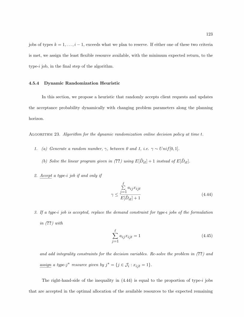
123
jobs of types k = 1, . . . , i− 1, exceeds what we plan to reserve. If either one of these two criteria
is met, we assign the least flexible resource available, with the minimum expected return, to the
type-i job, in the final step of the algorithm.
4.5.4 Dynamic Randomization Heuristic
In this section, we propose a heuristic that randomly accepts client requests and updates
the acceptance probability dynamically with changing problem parameters along the planning
horizon.
Algorithm 23. Algorithm for the dynamic randomization online decision policy at time t.
1. (a) Generate a random number, γ, between 0 and 1, i.e. γ ∼ Unif [0, 1].
(b) Solve the linear program given in (??) using E[Dit] + 1 instead of E[Dit].
2. Accept a type-i job if and only if
γ ≤
∑j=1
aijxijt
E[Dit] + 1(4.44)
3. If a type-i job is accepted, replace the demand constraint for type-ı jobs of the formulation
in (??) with
∑
j=1aijxijt = 1 (4.45)
and add integrality constraints for the decision variables. Re-solve the problem in (??) and
assign a type-j∗ resource given by j∗ = {j ∈ Ji : xijt = 1}.
The right-hand-side of the inequality in (4.44) is equal to the proportion of type-i jobs
that are accepted in the optimal allocation of the available resources to the expected remaining

124
demand. Algorithm 23 accepts the request for a type-i job with a probability estimated with this
proportion. If the job is accepted, we solve an integer program and assign the resource prescribed
in the optimal solution.
4.5.5 First-Come First-Served Policy
First-come first-served (FCFS) decision policy never rejects a request as long as there is at
least one resource that can be assigned to the requested job, and randomly assigns an available
resource. We use this simple policy as a benchmark for our heuristics in performance assessment.
Algorithm 24. Algorithm for the first-come first-served online decision policy at time t.
1. Accept a type-i job if
∑
j∈Ji
njt > 0. (4.46)
2. If a type-i job is accepted, assign any available resource that can handle the job.
4.6 Computational Results
We now present computational results for our online algorithms. Our two primary objec-
tives are:
• To verify the effectiveness and measure the performance of the online algorithms under
various operating conditions,
• To demonstrate the benefits of resource flexibility within the problem context
We wrote our simulation code in C, incorporating CPLEX 7.5 optimization subroutines, and
performed the computations on a dual processor WinNT server, with two Intel Pentium III Xeon
1.0 GHz processors and 2GB of RAM.
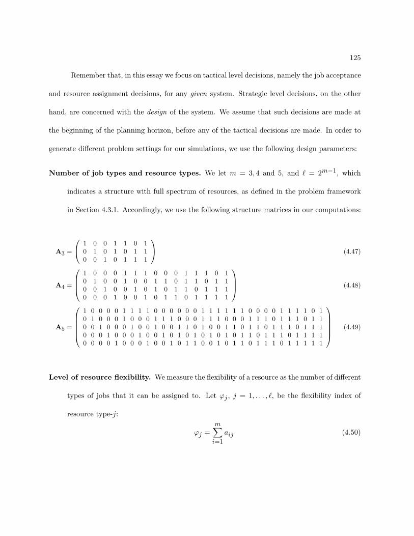
125
Remember that, in this essay we focus on tactical level decisions, namely the job acceptance
and resource assignment decisions, for any given system. Strategic level decisions, on the other
hand, are concerned with the design of the system. We assume that such decisions are made at
the beginning of the planning horizon, before any of the tactical decisions are made. In order to
generate different problem settings for our simulations, we use the following design parameters:
Number of job types and resource types. We let m = 3, 4 and 5, and ` = 2m−1, which
indicates a structure with full spectrum of resources, as defined in the problem framework
in Section 4.3.1. Accordingly, we use the following structure matrices in our computations:
A3 =
1 0 0 1 1 0 10 1 0 1 0 1 10 0 1 0 1 1 1
(4.47)
A4 =
1 0 0 0 1 1 1 0 0 0 1 1 1 0 10 1 0 0 1 0 0 1 1 0 1 1 0 1 10 0 1 0 0 1 0 1 0 1 1 0 1 1 10 0 0 1 0 0 1 0 1 1 0 1 1 1 1
(4.48)
A5 =
1 0 0 0 0 1 1 1 1 0 0 0 0 0 0 1 1 1 1 1 1 0 0 0 0 1 1 1 1 0 10 1 0 0 0 1 0 0 0 1 1 1 0 0 0 1 1 1 0 0 0 1 1 1 0 1 1 1 0 1 10 0 1 0 0 0 1 0 0 1 0 0 1 1 0 1 0 0 1 1 0 1 1 0 1 1 1 0 1 1 10 0 0 1 0 0 0 1 0 0 1 0 1 0 1 0 1 0 1 0 1 1 0 1 1 1 0 1 1 1 10 0 0 0 1 0 0 0 1 0 0 1 0 1 1 0 0 1 0 1 1 0 1 1 1 0 1 1 1 1 1
(4.49)
Level of resource flexibility. We measure the flexibility of a resource as the number of different
types of jobs that it can be assigned to. Let ϕj , j = 1, . . . , `, be the flexibility index of
resource type-j:
ϕj =m∑
i=1aij (4.50)

126
Consequently, the flexibility of the system at the beginning of the planning horizon, as
designed by the strategic level decision-maker, is computed by:
ϕ =
∑`j=1 ϕjnjT
∑`j=1 njT
(4.51)
If the system uses special-purpose resources exclusively, ϕ is equal to 1; conversely, if the
only type of resource in the system is a flexible resource that can be assigned to all types of
jobs, ϕ is equal to m, i.e. 1 ≤ ϕ ≤ m.
Resource availability. The ratio of the expected aggregate demand to the total number of
resources is an indication of the tightness of system capacity. Although this estimate is
rather crude, we use it to measure the availability of resources in the system. We define α
as,
α =
∑`j=1 njT∑m
i=1 E[DiT ](4.52)
Clearly, as the value of α increases, we expect to meet a larger proportion of the incoming
demand over the planning horizon.
Job revenues. We assume that the revenue of a type-i job is (100r)% larger than the revenue
of a type-(i + 1) job, i.e. πi/πi+1 = (1 + r), and the value of r is constant for all i,
i = 1, . . . , m− 1. Therefore,
πi = (1 + r)m−iπm, i = 1, . . . , m (4.53)
Demand process. We use two demand models in our computations:
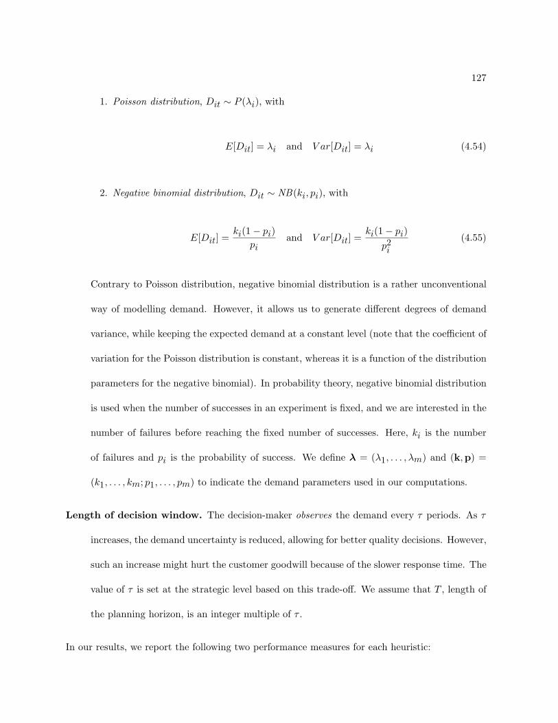
127
1. Poisson distribution, Dit ∼ P (λi), with
E[Dit] = λi and V ar[Dit] = λi (4.54)
2. Negative binomial distribution, Dit ∼ NB(ki, pi), with
E[Dit] =ki(1− pi)
piand V ar[Dit] =
ki(1− pi)p2i
(4.55)
Contrary to Poisson distribution, negative binomial distribution is a rather unconventional
way of modelling demand. However, it allows us to generate different degrees of demand
variance, while keeping the expected demand at a constant level (note that the coefficient of
variation for the Poisson distribution is constant, whereas it is a function of the distribution
parameters for the negative binomial). In probability theory, negative binomial distribution
is used when the number of successes in an experiment is fixed, and we are interested in the
number of failures before reaching the fixed number of successes. Here, ki is the number
of failures and pi is the probability of success. We define λ = (λ1, . . . , λm) and (k,p) =
(k1, . . . , km; p1, . . . , pm) to indicate the demand parameters used in our computations.
Length of decision window. The decision-maker observes the demand every τ periods. As τ
increases, the demand uncertainty is reduced, allowing for better quality decisions. However,
such an increase might hurt the customer goodwill because of the slower response time. The
value of τ is set at the strategic level based on this trade-off. We assume that T , length of
the planning horizon, is an integer multiple of τ .
In our results, we report the following two performance measures for each heuristic:
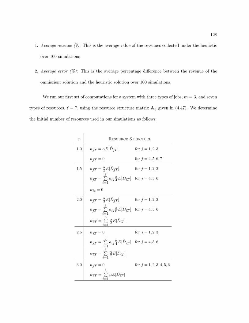
128
1. Average revenue ($): This is the average value of the revenues collected under the heuristic
over 100 simulations
2. Average error (%): This is the average percentage difference between the revenue of the
omniscient solution and the heuristic solution over 100 simulations.
We run our first set of computations for a system with three types of jobs, m = 3, and seven
types of resources, ` = 7, using the resource structure matrix A3 given in (4.47). We determine
the initial number of resources used in our simulations as follows:
ϕ Resource Structure
1.0 njT = αE[DjT ] for j = 1, 2, 3
njT = 0 for j = 4, 5, 6, 7
1.5 njT = α2 E[DjT ] for j = 1, 2, 3
njT =3∑
i=1aij
α4 E[DiT ] for j = 4, 5, 6
n7t = 0
2.0 njT = α3 E[DjT ] for j = 1, 2, 3
njT =3∑
i=1aij
α6 E[DiT ] for j = 4, 5, 6
n7T =3∑
i=1
α3 E[DiT ]
2.5 njT = 0 for j = 1, 2, 3
njT =3∑
i=1aij
α4 E[DiT ] for j = 4, 5, 6
n7T =3∑
i=1
α2 E[DiT ]
3.0 njT = 0 for j = 1, 2, 3, 4, 5, 6
n7T =3∑
i=1αE[DiT ]
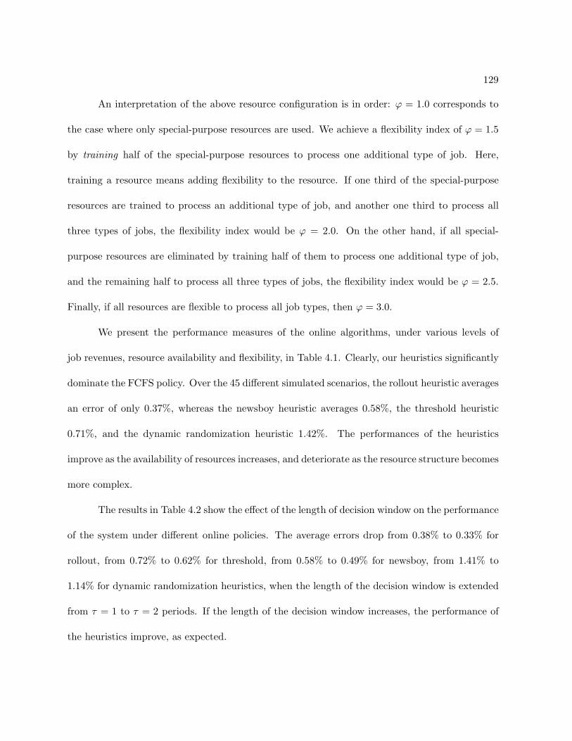
129
An interpretation of the above resource configuration is in order: ϕ = 1.0 corresponds to
the case where only special-purpose resources are used. We achieve a flexibility index of ϕ = 1.5
by training half of the special-purpose resources to process one additional type of job. Here,
training a resource means adding flexibility to the resource. If one third of the special-purpose
resources are trained to process an additional type of job, and another one third to process all
three types of jobs, the flexibility index would be ϕ = 2.0. On the other hand, if all special-
purpose resources are eliminated by training half of them to process one additional type of job,
and the remaining half to process all three types of jobs, the flexibility index would be ϕ = 2.5.
Finally, if all resources are flexible to process all job types, then ϕ = 3.0.
We present the performance measures of the online algorithms, under various levels of
job revenues, resource availability and flexibility, in Table 4.1. Clearly, our heuristics significantly
dominate the FCFS policy. Over the 45 different simulated scenarios, the rollout heuristic averages
an error of only 0.37%, whereas the newsboy heuristic averages 0.58%, the threshold heuristic
0.71%, and the dynamic randomization heuristic 1.42%. The performances of the heuristics
improve as the availability of resources increases, and deteriorate as the resource structure becomes
more complex.
The results in Table 4.2 show the effect of the length of decision window on the performance
of the system under different online policies. The average errors drop from 0.38% to 0.33% for
rollout, from 0.72% to 0.62% for threshold, from 0.58% to 0.49% for newsboy, from 1.41% to
1.14% for dynamic randomization heuristics, when the length of the decision window is extended
from τ = 1 to τ = 2 periods. If the length of the decision window increases, the performance of
the heuristics improve, as expected.
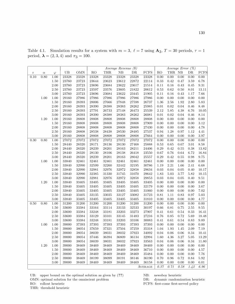
130
Table 4.1. Simulation results for a system with m = 3, ` = 7 using A3, T = 30 periods, τ = 1period, λ = (2, 3, 4) and π3 = 100.
Average Revenue ($) Average Error (%)r α ϕ UB OMN RO THR NB DR FCFS RO THR NB DR FCFS
0.10 0.80 1.00 23328 23328 23328 23328 23328 23328 23328 0.00 0.00 0.00 0.00 0.001.50 23760 23723 23644 23623 23612 22872 22114 0.33 0.42 0.47 3.59 6.782.00 23760 23723 23696 23684 23622 23617 21514 0.11 0.16 0.43 0.45 9.312.50 23760 23723 23597 23576 23605 21822 20612 0.53 0.62 0.50 8.01 13.113.00 23760 23723 23696 23684 23622 23445 21905 0.11 0.16 0.43 1.17 7.66
1.00 1.00 29160 27986 27986 27986 27986 27986 27986 0.00 0.00 0.00 0.00 0.001.50 29160 28393 28006 27666 27848 27598 26737 1.36 2.56 1.92 2.80 5.832.00 29160 28393 28390 28388 28383 28262 25985 0.01 0.02 0.04 0.46 8.482.50 29160 28393 27791 26733 27148 26473 25539 2.12 5.85 4.38 6.76 10.053.00 29160 28393 28390 28388 28383 28262 26081 0.01 0.02 0.04 0.46 8.14
1.20 1.00 29160 28808 28808 28808 28808 28808 28808 0.00 0.00 0.00 0.00 0.001.50 29160 28808 28808 28808 28808 28808 27909 0.00 0.00 0.00 0.00 3.122.00 29160 28808 28808 28808 28808 28808 27430 0.00 0.00 0.00 0.00 4.782.50 29160 28808 28538 28438 28530 28485 27537 0.94 1.28 0.97 1.12 4.413.00 29160 28808 28808 28808 28808 28808 27664 0.00 0.00 0.00 0.00 3.97
0.30 0.80 1.00 27072 27072 27072 27072 27072 27072 27072 0.00 0.00 0.00 0.00 0.001.50 28440 28320 28171 28136 28130 27468 25888 0.53 0.65 0.67 3.01 8.582.00 28440 28320 28239 28201 28163 28211 24406 0.29 0.42 0.55 0.38 13.822.50 28440 28320 28130 28106 28138 26418 23550 0.67 0.76 0.64 6.72 16.843.00 28440 28320 28239 28201 28163 28042 25557 0.29 0.42 0.55 0.98 9.75
1.00 1.00 33840 32461 32461 32461 32461 32461 32461 0.00 0.00 0.00 0.00 0.001.50 33840 32990 32599 32260 32442 32195 30786 1.19 2.21 1.66 2.41 6.682.00 33840 32990 32981 32976 32972 32858 29634 0.03 0.04 0.05 0.40 10.172.50 33840 32990 32385 31330 31745 31070 29642 1.83 5.03 3.77 5.82 10.153.00 33840 32990 32981 32976 32972 32858 29853 0.03 0.04 0.05 0.40 9.51
1.20 1.00 33840 33405 33405 33405 33405 33405 33405 0.00 0.00 0.00 0.00 0.001.50 33840 33405 33405 33405 33405 33405 32179 0.00 0.00 0.00 0.00 3.672.00 33840 33405 33405 33405 33405 33405 31060 0.00 0.00 0.00 0.00 7.022.50 33840 33405 33135 33035 33127 33082 31723 0.81 1.11 0.83 0.97 5.033.00 33840 33405 33405 33405 33405 33405 31810 0.00 0.00 0.00 0.00 4.77
0.50 0.80 1.00 31200 31200 31200 31200 31200 31200 31200 0.00 0.00 0.00 0.00 0.001.50 33600 33384 33164 33114 33133 32533 30197 0.66 0.81 0.75 2.55 9.552.00 33600 33384 33248 33181 33203 33273 27907 0.41 0.61 0.54 0.33 16.412.50 33600 33384 33129 33101 33145 31483 27216 0.76 0.85 0.72 5.69 18.483.00 33600 33384 33248 33181 33203 33106 30083 0.41 0.61 0.54 0.83 9.89
1.00 1.00 39000 37393 37393 37393 37393 37393 37393 0.00 0.00 0.00 0.00 0.001.50 39000 38054 37659 37321 37504 37259 35318 1.04 1.93 1.45 2.09 7.192.00 39000 38054 38039 38031 38032 37923 34092 0.04 0.06 0.06 0.34 10.412.50 39000 38054 37446 36394 36809 36134 32994 1.60 4.36 3.27 5.05 13.293.00 39000 38054 38039 38031 38032 37923 33563 0.04 0.06 0.06 0.34 11.80
1.20 1.00 39000 38469 38469 38469 38469 38469 38469 0.00 0.00 0.00 0.00 0.001.50 39000 38469 38469 38469 38469 38469 36710 0.00 0.00 0.00 0.00 4.572.00 39000 38469 38469 38469 38469 38469 35484 0.00 0.00 0.00 0.00 7.762.50 39000 38469 38199 38099 38191 38146 36190 0.70 0.96 0.72 0.84 5.923.00 39000 38469 38469 38469 38469 38469 36158 0.00 0.00 0.00 0.00 6.01
Average 0.37 0.71 0.58 1.42 6.96
UB: upper bound on the optimal solution as given by (??) NB: newsboy heuristicOMN: optimal solution for the omniscient problem DR: dynamic randomization heuristicRO: rollout heuristic FCFS: first-come first-served policyTHR: threshold heuristic

131
Table 4.2. Simulation results for a system with m = 3, ` = 7 using A3, T = 30 periods,λ = (2, 3, 4), π3 = 100 and r = 0.3.
Average Revenue ($) Average Error (%)τ α ϕ OMN RO THR NB DR FCFS RO THR NB DR FCFS1 0.80 1.00 27072 27072 27072 27072 27072 27072 0.00 0.00 0.00 0.00 0.00
1.50 28320 28171 28136 28130 27468 25888 0.53 0.65 0.67 3.01 8.582.00 28320 28239 28201 28163 28211 24406 0.29 0.42 0.55 0.38 13.822.50 28320 28130 28106 28138 26418 23550 0.67 0.76 0.64 6.72 16.843.00 28320 28239 28201 28163 28042 25557 0.29 0.42 0.55 0.98 9.75
1.00 1.00 32461 32461 32461 32461 32461 32461 0.00 0.00 0.00 0.00 0.001.50 32990 32599 32260 32442 32195 30786 1.19 2.21 1.66 2.41 6.682.00 32990 32981 32976 32972 32858 29634 0.03 0.04 0.05 0.40 10.172.50 32990 32385 31330 31745 31070 29642 1.83 5.03 3.77 5.82 10.153.00 32990 32981 32976 32972 32858 29853 0.03 0.04 0.05 0.40 9.51
1.20 1.00 33405 33405 33405 33405 33405 33405 0.00 0.00 0.00 0.00 0.001.50 33405 33405 33405 33405 33405 32179 0.00 0.00 0.00 0.00 3.672.00 33405 33405 33405 33405 33405 31060 0.00 0.00 0.00 0.00 7.022.50 33405 33135 33035 33127 33082 31723 0.81 1.11 0.83 0.97 5.033.00 33405 33405 33405 33405 33405 31810 0.00 0.00 0.00 0.00 4.77
Average 0.38 0.72 0.58 1.41 7.102 0.80 1.00 27072 27072 27072 27072 27072 27072 0.00 0.00 0.00 0.00 0.00
1.50 28400 28270 28247 28242 27677 26659 0.46 0.54 0.55 2.54 6.132.00 28400 28320 28280 28279 28294 25216 0.28 0.42 0.43 0.37 11.212.50 28400 28236 28214 28254 26854 24594 0.58 0.65 0.51 5.44 13.403.00 28400 28333 28305 28259 28125 26210 0.23 0.33 0.49 0.97 7.71
1.00 1.00 33262 33262 33262 33262 33262 33262 0.00 0.00 0.00 0.00 0.001.50 33220 32909 32511 32799 32583 31000 0.94 2.13 1.26 1.92 6.682.00 33220 33212 33207 33202 33116 30240 0.02 0.04 0.05 0.31 8.972.50 33220 32637 31808 32143 31705 30509 1.75 4.25 3.24 4.56 8.163.00 33220 33211 33209 33205 33119 30944 0.03 0.03 0.04 0.30 6.85
1.20 1.00 33420 33420 33420 33420 33420 33420 0.00 0.00 0.00 0.00 0.001.50 33420 33420 33420 33420 33420 33042 0.00 0.00 0.00 0.00 1.132.00 33420 33420 33420 33420 33420 31996 0.00 0.00 0.00 0.00 4.262.50 33420 33196 33133 33155 33168 32210 0.67 0.86 0.79 0.75 3.623.00 33420 33420 33420 33420 33420 32738 0.00 0.00 0.00 0.00 2.04
Average 0.33 0.62 0.49 1.14 5.34

132
In Table 4.3, we provide a comparison of the heuristics under different levels of demand
variability. In all three cases, the expected values of per period demands are approximately equal
to 2, 3 and 4 for type-1, type-2 and type-3 jobs, respectively. However, the coefficient of variation
(the ratio of standard deviation to mean) of the demands increase from case 1 to case 3 (case 1
having the smallest variance and case 3 having the largest). Notice that, rollout, threshold and
dynamic randomization heuristics are affected adversely from increased variability, since they do
not consider demand variance in their algorithms. On the other hand, the newsboy heuristic
is more tolerant to variance, as the algorithm uses the probability distribution of the demands
instead of their expected values. Further, it has the best overall performance among all heuristics
(newsboy heuristic has an average error of 0.86% whereas threshold heuristic has an average error
of 1.19%, rollout heuristic 1.58%, and dynamic randomization heuristic 3.17%).
Table 4.3. Simulation results for a system with m = 3, ` = 7 using A3, T = 30 periods, τ = 1period, ϕ = 2.5, α = 0.8, π3 = 100 and r = 0.3.
Average Revenue ($) Average Error (%)Case k p OMN RO THR NB DR FCFS RO THR NB DR FCFS
1 (4,3,3) (0.66,0.50,0.43) 28277 27987 28012 28048 27398 23398 1.03 0.94 0.81 3.11 17.252 (2,2,2) (0.50,0.40,0.33) 28288 27813 27923 28021 27410 23185 1.68 1.29 0.94 3.10 18.043 (1,1,1) (0.33,0.25,0.20) 28185 27613 27809 27952 27258 22810 2.03 1.33 0.83 3.29 19.07
Average 1.58 1.19 0.86 3.17 18.12
Next, we simulate a system with four types of jobs and fifteen types of resources using the
structure matrix A4 given in (4.48), under different levels of resource availability and flexibility,
and report our results in Table 4.4. We assume that, in a system with flexibility index ϕ, only
resource types with flexibility indices ϕj = ϕ are available. Consequently, we determine the

133
Table 4.4. Simulation results for a system with m = 4, ` = 15 using A4, T = 20 periods,λ = (1, 2, 3, 4), π4 = 100 and r = 0.2.
Average Revenue ($) Average Error (%)α ϕ UB OMN RO THR NB DR FCFS RO THR NB DR FCFS0.6 1 21974 21974 21974 21974 21974 21974 21974 0.00 0.00 0.00 0.00 0.00
2 24624 24621 24367 24074 23929 23500 21135 1.03 1.20 0.6 1.79 10.063 24624 24621 24443 24230 24116 23814 20996 0.72 0.87 0.47 1.25 11.834 24624 24621 24497 24340 24254 24154 20939 0.5 0.64 0.35 0.41 13.31
0.8 1 29299 29299 29299 29299 29299 29299 29299 0.00 0.00 0.00 0.00 0.002 30624 30556 30204 29760 29393 28575 27189 1.15 1.47 1.23 2.78 4.853 30624 30556 30323 30056 29803 29257 27592 0.76 0.88 0.84 1.83 5.694 30624 30556 30400 30217 30071 29884 27723 0.51 0.60 0.48 0.62 7.23
1.0 1 36624 34869 34869 34869 34869 34869 34869 0.00 0.00 0.00 0.00 0.002 36624 36046 35303 34113 33113 32083 29080 2.06 3.37 2.93 3.11 9.363 36624 36046 35638 34636 33804 32810 30903 1.13 2.81 2.40 2.94 5.814 36624 36046 36009 35965 35943 35626 34461 0.10 0.12 0.06 0.88 3.27
Average 0.66 1.00 0.78 1.30 5.96
number of type-j resources using:
njT =4∑
i=1aij
α
ϕjE[DiT ]
Over 12 different scenarios, the average error is equal to 0.66% for the rollout heuristic, 1.00% for
the threshold heuristic, 0.78% for the newsboy heuristic, and 1.30% for the dynamic randomization
heuristic, compared to the 5.96% average error of the FCFS policy. Note also that, the average
revenue collected increases with flexibility, as expected. Our findings from a larger system with
five types of jobs and thirty one types of resources, as presented in Table 4.5, support these claims.
Observations from this computational study are:
• Our heuristics solve the problem effectively, and are near-optimal in many cases.
• All heuristics are superior to the FCFS policy, confirming the fact that acceptance and
assignment decisions are critical, and better decisions yield to considerably larger revenues.

134
Table 4.5. Simulation results for a system with m = 5, ` = 31 using A5, T = 24 periods,λ = (1, 2, 3, 4, 5), π5 = 100 and r = 0.2.
Average Revenue ($) Average Error (%)α ϕ UB OMN RO THR NB DR FCFS RO THR NB DR FCFS0.5 1 23578 23578 23578 23578 23578 23578 23578 0.00 0.00 0.00 0.00 0.00
2 27956 27799 27546 27490 27554 27384 23479 0.91 1.11 0.88 1.49 15.543 27956 27956 27673 27637 27723 27707 22856 1.01 1.14 0.83 0.89 18.244 27956 27956 27749 27726 27796 27819 22641 0.74 0.82 0.57 0.49 19.015 27956 27956 27771 27735 27805 27891 22364 0.66 0.79 0.54 0.23 20.00
0.75 1 35367 35336 35336 35336 35336 35336 35336 0.00 0.00 0.00 0.00 0.002 38156 38156 37778 37595 37835 36751 35206 0.99 1.47 0.84 3.68 7.733 38156 38156 37770 37736 37812 37377 34409 1.01 1.10 0.9 2.04 9.824 38156 38156 37919 37991 38007 37827 33539 0.62 0.43 0.39 0.86 12.15 38156 38182 38143 38071 38090 38063 32893 0.1 0.29 0.24 0.31 13.85
1 1 47156 45093 45093 45093 45093 45093 45093 0.00 0.00 0.00 0.00 0.002 47156 46623 46035 44837 45298 44706 40967 1.26 3.83 2.84 4.11 12.133 47156 46623 46170 45331 45807 44935 43005 0.97 2.77 1.75 3.62 7.764 47156 46623 46245 46138 46240 46058 44744 0.81 1.04 0.82 1.21 4.035 47156 46623 46445 46604 46613 46347 45354 0.38 0.04 0.02 0.59 2.72
Average 0.63 0.99 0.71 1.30 9.53
• Among the proposed heuristics, the rollout heuristic outperforms the others in many problem
instances. However, the newsboy and threshold heuristics are also competitive.
• The newsboy heuristic is capable of managing large levels of demand variance, and is the
best heuristic under such circumstances.
• Threshold heuristic performs remarkably considering that it is a very simple and easy-to-
implement decision rule.
• The upper bound proposed in Section 4.4.4 gets tighter as the level of resource availability
increases.
• Added resource flexibility increases revenues, however is more valuable under tighter resource
constraints.

135
• The increase in the average omniscient revenue diminishes significantly as the flexibility
index increases, and does not add any value beyond a certain point. Therefore, “a little
flexibility goes a long way”.
4.7 Conclusions and Future Research
The contributions of this essay are as follows:
1. We extend the practice of revenue management to a new application area, the workplace
learning industry, and model the associated revenue maximization problem as a stochastic
dynamic program.
2. Since the dynamic program is doomed with the curse of dimensionality (Bellman 1961), we
initially study several special cases of the problem and identify their optimal policies.
3. Based on our insights from the special case analysis, we propose efficient heuristics as an
approximate solution to the general problem.
4. We present computational results to assess the performance of our heuristics for different
problem settings. Through an extensive simulation study, we show that our heuristics
effectively solve the problem and significantly dominate the benchmark policy of choice
(FCFS).
For our future research, we would like to consider incorporating the strategic level decisions,
which are basically concerned with the initial design of the system, into the problem. Determining
the initial structure of resources, and the capacity to be acquired remains to be an interesting
aspect of the problem. Another path we could follow is the extension of the problem to the

136
rolling time horizon scenario, where each job can be handled at any time on the time line, and
the resource assigned to the job can be kept busy for a certain duration.

137
Appendix
Proof of Proposition 14
We use induction on t to prove the first two parts of the proposition. For period k = 1:
∆21(n1, n3) = u1(n1, 0, n3 + 1; e2)− u1(n1, 0, n3; e2)
=
π2 if n3 = 0
0 if n3 > 0
and
∆(n1, n3) = u1(n1, 0, n3 + 1)− u1(n1, 0, n3)
=
p1π1 + p2π2 if n1 = 0, n3 = 0
p2π2 if n1 > 0, n3 = 0
0 if n1 ≥ 0, n3 > 0
Obviously, the proposition is true for k = 1. Now, we assume that the proposition holds for
k = 1, . . . , t− 1. We first show that ∆2t (n1, 1) ≤ ∆2
t (n1, 0) for any given n1.
∆2t (n1, 1) = ut(n1, 0, 2; e2)− ut(n1, 0, 1; e2)
= max{π2 + ut−1(n1, 0, 1), ut−1(n1, 0, 2)} −max{π2 + ut−1(n1, 0, 0), ut−1(n1, 0, 1)}
= max{π2, ut−1(n1, 0, 2)− ut−1(n1, 0, 1)} −max{π2 + ut−1(n1, 0, 0)− ut−1(n1, 0, 1), 0}
= max{π2, ∆t−1(n1, 1)} −max{π2 −∆t−1(n1, 0), 0}
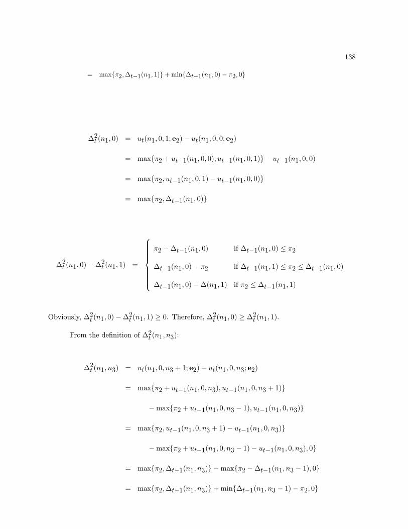
138
= max{π2, ∆t−1(n1, 1)}+ min{∆t−1(n1, 0)− π2, 0}
∆2t (n1, 0) = ut(n1, 0, 1; e2)− ut(n1, 0, 0; e2)
= max{π2 + ut−1(n1, 0, 0), ut−1(n1, 0, 1)} − ut−1(n1, 0, 0)
= max{π2, ut−1(n1, 0, 1)− ut−1(n1, 0, 0)}
= max{π2, ∆t−1(n1, 0)}
∆2t (n1, 0)−∆2
t (n1, 1) =
π2 −∆t−1(n1, 0) if ∆t−1(n1, 0) ≤ π2
∆t−1(n1, 0)− π2 if ∆t−1(n1, 1) ≤ π2 ≤ ∆t−1(n1, 0)
∆t−1(n1, 0)−∆(n1, 1) if π2 ≤ ∆t−1(n1, 1)
Obviously, ∆2t (n1, 0)−∆2
t (n1, 1) ≥ 0. Therefore, ∆2t (n1, 0) ≥ ∆2
t (n1, 1).
From the definition of ∆2t (n1, n3):
∆2t (n1, n3) = ut(n1, 0, n3 + 1; e2)− ut(n1, 0, n3; e2)
= max{π2 + ut−1(n1, 0, n3), ut−1(n1, 0, n3 + 1)}
−max{π2 + ut−1(n1, 0, n3 − 1), ut−1(n1, 0, n3)}
= max{π2, ut−1(n1, 0, n3 + 1)− ut−1(n1, 0, n3)}
−max{π2 + ut−1(n1, 0, n3 − 1)− ut−1(n1, 0, n3), 0}
= max{π2, ∆t−1(n1, n3)} −max{π2 −∆t−1(n1, n3 − 1), 0}
= max{π2, ∆t−1(n1, n3)}+ min{∆t−1(n1, n3 − 1)− π2, 0}

139
Based on our hypothesis, both ∆t−1(n1, n3) and ∆t−1(n1, n3 − 1) are nonincreasing functions
of n1 and n3. Therefore, max{π2, ∆t−1(n1, n3)} and min{∆t−1(n1, n3 − 1) − π2, 0} are also
nonincreasing in n1 and n3. Consequently, ∆2t (n1, n3) is nonincreasing in n1 and n3.
From the definition of ∆t(n1, n3), we obtain the following:
∆t(n1, n3) = ut(n1, n3 + 1)− ut(n1, n3)
=
p1π1 + p2∆2t (0, 0) + (1− p1 − p2)∆t−1(0, 0) if n1 = 0, n3 = 0
p1∆t−1(0, n3 − 1) + p2∆2t (0, n3) + (1− p1 − p2)∆t−1(0, n3) if n1 = 0, n3 > 0
p1∆t−1(n1 − 1, n3) + p2∆2t (n1, n3) + (1− p1 − p2)∆t−1(n1, n3) if n1 > 0
From the above expression, one can easily find that ∆t(0, 1) ≤ ∆t(0, 0) and ∆t(1, 0) ≤
∆t(0, 0), using the relationships ∆t−1(0, 0) ≤ π1, ∆2t (0, 1) ≤ ∆2
t (0, 1) ≤ ∆2t (0, 0), ∆2
t (1, 0) ≤
∆2t (0, 0) and our hypothesis ∆t−1(0, 1) ≤ ∆t−1(0, 0) and ∆t−1(1, 0) ≤ ∆t−1(0, 0). In conclusion,
∆t(n1, n3) is a nonincreasing function of n1 and n3, since ∆2t (n1, n3), ∆t−1(n1 − 1, n3) and
∆t−1(n1, n3) are all nonincreasing functions of n1 and n3.
Next, we prove the third part of the proposition by studying all possible cases of n1 and
n3.
Case 1. n1 = 0 and n3 = 0
∆t(0, 0) = ut(0, 0, 1)− ut(0, 0, 0)
= p1π1 + p2 max{π2, ut−1(0, 0, 1)}+ (1− p1 − p2)ut−1(0, 0, 1)
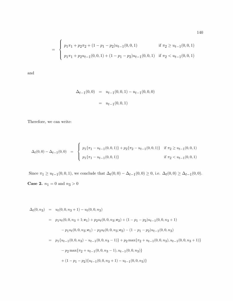
140
=
p1π1 + p2π2 + (1− p1 − p2)ut−1(0, 0, 1) if π2 ≥ ut−1(0, 0, 1)
p1π1 + p2ut−1(0, 0, 1) + (1− p1 − p2)ut−1(0, 0, 1) if π2 < ut−1(0, 0, 1)
and
∆t−1(0, 0) = ut−1(0, 0, 1)− ut−1(0, 0, 0)
= ut−1(0, 0, 1)
Therefore, we can write:
∆t(0, 0)−∆t−1(0, 0) =
p1{π1 − ut−1(0, 0, 1)}+ p2{π2 − ut−1(0, 0, 1)} if π2 ≥ ut−1(0, 0, 1)
p1{π1 − ut−1(0, 0, 1)} if π2 < ut−1(0, 0, 1)
Since π1 ≥ ut−1(0, 0, 1), we conclude that ∆t(0, 0)−∆t−1(0, 0) ≥ 0, i.e. ∆t(0, 0) ≥ ∆t−1(0, 0).
Case 2. n1 = 0 and n3 > 0
∆t(0, n3) = ut(0, 0, n3 + 1)− ut(0, 0, n3)
= p1ut(0, 0, n3 + 1; e1) + p2ut(0, 0, n3; e2) + (1− p1 − p2)ut−1(0, 0, n3 + 1)
− p1ut(0, 0, n3; e1)− p2ut(0, 0, n3; e2)− (1− p1 − p2)ut−1(0, 0, n3)
= p1{ut−1(0, 0, n3)− ut−1(0, 0, n3 − 1)}+ p2 max{π2 + ut−1(0, 0, n3), ut−1(0, 0, n3 + 1)}
− p2 max{π2 + ut−1(0, 0, n3 − 1), ut−1(0, 0, n3)}
+ (1− p1 − p2){ut−1(0, 0, n3 + 1)− ut−1(0, 0, n3)}
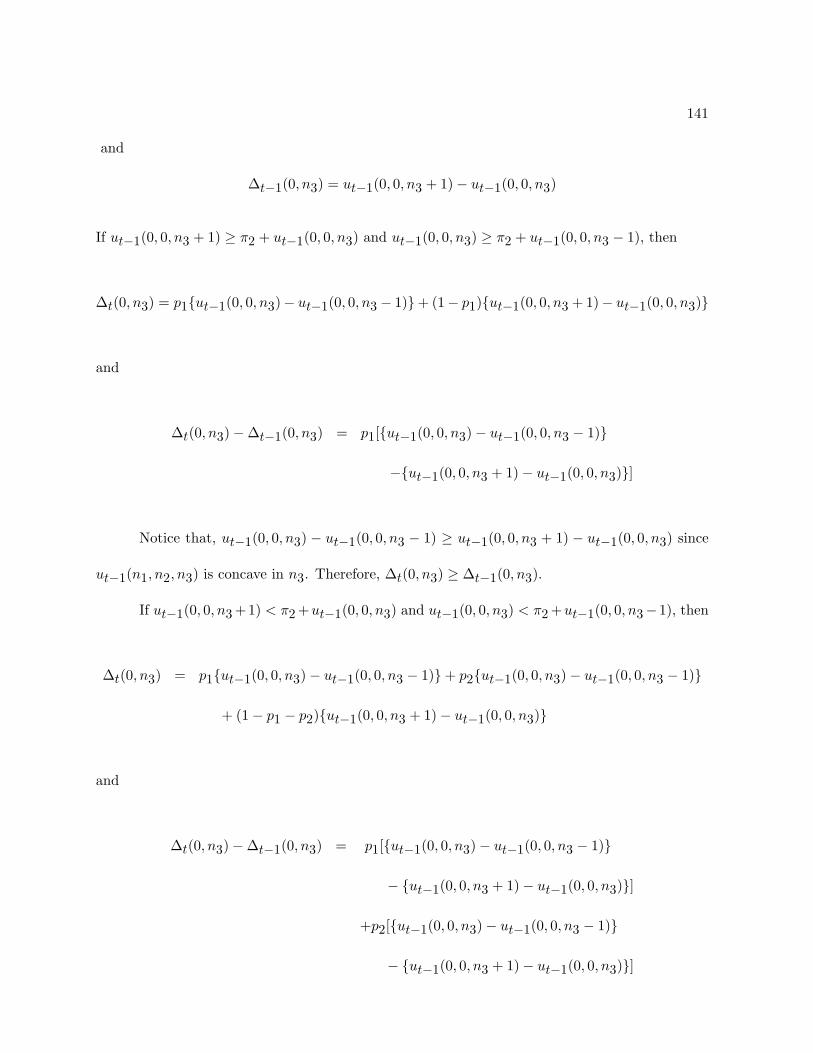
141
and
∆t−1(0, n3) = ut−1(0, 0, n3 + 1)− ut−1(0, 0, n3)
If ut−1(0, 0, n3 + 1) ≥ π2 + ut−1(0, 0, n3) and ut−1(0, 0, n3) ≥ π2 + ut−1(0, 0, n3 − 1), then
∆t(0, n3) = p1{ut−1(0, 0, n3)− ut−1(0, 0, n3 − 1)}+ (1− p1){ut−1(0, 0, n3 + 1)− ut−1(0, 0, n3)}
and
∆t(0, n3)−∆t−1(0, n3) = p1[{ut−1(0, 0, n3)− ut−1(0, 0, n3 − 1)}
−{ut−1(0, 0, n3 + 1)− ut−1(0, 0, n3)}]
Notice that, ut−1(0, 0, n3) − ut−1(0, 0, n3 − 1) ≥ ut−1(0, 0, n3 + 1) − ut−1(0, 0, n3) since
ut−1(n1, n2, n3) is concave in n3. Therefore, ∆t(0, n3) ≥ ∆t−1(0, n3).
If ut−1(0, 0, n3 +1) < π2 +ut−1(0, 0, n3) and ut−1(0, 0, n3) < π2 +ut−1(0, 0, n3−1), then
∆t(0, n3) = p1{ut−1(0, 0, n3)− ut−1(0, 0, n3 − 1)}+ p2{ut−1(0, 0, n3)− ut−1(0, 0, n3 − 1)}
+ (1− p1 − p2){ut−1(0, 0, n3 + 1)− ut−1(0, 0, n3)}
and
∆t(0, n3)−∆t−1(0, n3) = p1[{ut−1(0, 0, n3)− ut−1(0, 0, n3 − 1)}
− {ut−1(0, 0, n3 + 1)− ut−1(0, 0, n3)}]
+p2[{ut−1(0, 0, n3)− ut−1(0, 0, n3 − 1)}
− {ut−1(0, 0, n3 + 1)− ut−1(0, 0, n3)}]
142
Notice that, ut−1(0, 0, n3)− ut−1(0, 0, n3 − 1) ≥ ut−1(0, 0, n3 + 1)− ut−1(0, 0, n3), since
ut−1(n1, n2, n3) is concave in n3. Therefore, ∆t(0, n3) ≥ ∆t−1(0, n3).
Finally, if ut−1(0, 0, n3 + 1) < π2 + ut−1(0, 0, n3) and ut−1(0, 0, n3) > π2 + ut−1(0, 0, n3 − 1),
then
∆t(0, n3) = p1{ut−1(0, 0, n3)− ut−1(0, 0, n3 − 1)}+ p2π2
+ (1− p1 − p2){ut−1(0, 0, n3 + 1)− ut−1(0, 0, n3)}
and
∆t(0, n3)−∆t−1(0, n3) = p1[{ut−1(0, 0, n3)− ut−1(0, 0, n3 − 1)}
− {ut−1(0, 0, n3 + 1)− ut−1(0, 0, n3)}]
+p2[π2 − {ut−1(0, 0, n3 + 1)− ut−1(0, 0, n3)}]
Notice that ∆t(0, n3)−∆t−1(0, n3) ≥ 0 since ut−1(0, 0, n3)−ut−1(0, 0, n3−1) ≥ ut−1(0, 0, n3 +
1)− ut−1(0, 0, n3) due to the concavity of ut−1(n1, n2, n3) with respect to n3.
Finally, we do not consider the scenario where ut−1(0, 0, n3 + 1) > π2 + ut−1(0, 0, n3) and
ut−1(0, 0, n3) < π2 + ut−1(0, 0, n3 − 1), because ut−1(n1, n2, n3) is concave in n3.
Case 3. n1 > 0 and n3 > 0
∆t(n1, n3) = ut(n1, 0, n3 + 1)− ut(n1, 0, n3)
= p1ut(n1, 0, n3 + 1; e1) + p2ut(n1, 0, n3 + 1; e2) + (1− p1 − p2)ut−1(n1, 0, n3 + 1)
− p1ut(n1, 0, n3; e1) + p2ut(n1, 0, n3; e2) + (1− p1 − p2)ut−1(n1, 0, n3)
= p1{ut−1(n1 − 1, 0, n3 + 1)− ut−1(n1 − 1, 0, n3)}

143
− p2{ut(n1, 0, n3 + 1; e2)− ut(n1, 0, n3; e2)}
+ (1− p1 − p2){ut−1(n1, 0, n3 + 1)− ut−1(n1, 0, n3)}
and
∆t−1(n1, n3) = ut−1(n1, 0, n3 + 1)− ut−1(n1, 0, n3)
We can show that ∆t(n1, n3) ≥ ∆t−1(n1, n3) with a very similar approach to the one in the
previous case. However, in the process we need to use the following relationship:
ut−1(n1 − 1, 0, n3 + 1)− ut−1(n1 − 1, 0, n3) ≥ ut−1(n1, 0, n3 + 1)− ut−1(n1, 0, n3)
The above expression, which is equivalent to ∆t−1(n1 − 1, n3) ≥ ∆t−1(n1, n3), is valid since
∆t−1(n1, n3) is a nonincreasing function of n3.
Finally, we establish the result in the last part of the proposition by induction. For period
k = 1:
∆21(n1, n3) =
π2 if n3 = 0
0 if n3 > 0
and
∆1(n1 + 1, n3 − 1) =
π2 if n3 = 1
0 if n3 ≥ 2
144
Thus, the proposition holds for k = 1. We now assume that, the result is also true for k =
2, . . . , t− 1. For n3 = 1, we have:
∆2t (n1, 1) = ut(n1, 0, 2; e2)− ut(n1, 0, 1; e2)
= max{π2 + ut−1(n1, 0, 1), ut−1(n1, 0, 2)} −max{π2 + ut−1(n1, 0, 0), ut−1(n1, 0, 1)}
= max{π2, ∆t−1(n1, 1)}+ min{∆t−1(n1, 0)− π2, 0}
and
∆2t (n1 + 1, 0) = ut(n1 + 1, 0, 1; e2)− ut(n1 + 1, 0, 0; e2)
= max{π2 + ut−1(n1 + 1, 0, 0), ut−1(n1 + 1, 0, 1)} − ut−1(n1 + 1, 0, 0)
= max{π2,∆t−1(n1 + 1, 0)}
Therefore,
∆2t (n1 + 1, 0)−∆2
t (n1, 1) =
π2 −∆t−1(n1, 0) if ∆t−1(n1, 0) ≤ π2
max{π2, ∆t−1(n1 + 1, 0)}
−max{π2, ∆t−1(n1, 1)}if ∆t−1(n1, 0) > π2
Note that ∆2t (n1 + 1, 0) −∆2
t (n1, 1) ≥ 0. Thus, ∆2t (n1 + 1, 0) ≥ ∆2
t (n1, 1). On the other hand,
for n3 > 1, we have:
∆2t (n1, n3) = max{π2, ∆t−1(n1, n3)}+ min{∆t−1(n1, n3 − 1)− π2, 0}

145
and
∆2t (n1 + 1, n3 − 1) = max{π2, ∆t−1(n1 + 1, n3 − 1)}+ min{∆t−1(n1 + 1, n3 − 2)− π2, 0}
Based on our initial assumption, we know that max{π2, ∆t−1(n1, n3)} ≤ max{π2, ∆t−1(n1 +
1, n3−1)} and min{∆t−1(n1, n3−1)−π2, 0} ≤ min{∆t−1(n1 +1, n−3−2)−π2, 0}. As a result,
∆2t (n1, n2) ≤ ∆2
t (n1 + 1, n3 − 1). This completes the proof of the first part of the proposition.
From the definition of ∆t(n1, n3), we can write:
∆t(n1, n3) = ut(n1, n3 + 1)− ut(n1, n3)
=
p1π1 + p2∆2t (0, 0) + (1− p1 − p2)∆t(0, 0) if n1 = 0, n3 = 0
p1∆t−1(0, n3 − 1) + p2∆2t (0, n3)
+ (1− p1 − p2)∆t−1(0, n3)if n1 = 0, n3 > 0
p1∆t−1(n1 − 1, n3) + p2∆2t (n1, n3)
+ (1− p1 − p2)∆t−1(n1, n3)if n1 > 0
If n1 = 0 and n3 = 0, then
∆t(n1 + 1, n3 − 1)−∆t(n1, n3) = p2[∆2t (1, 0)−∆2
t (0, 1)]
+ (1− p1 − p2)[∆2t−1(1, 0)−∆2
t−1(0, 1)]
If n1 = 0 and n3 > 0, then
∆t(n1 + 1, n3 − 1)−∆t(n1, n3) = p2[∆2t (1, n3 − 1)−∆2
t (0, n3)]
+ (1− p1 − p2)[∆t−1(1, n3 − 1)−∆t(0, n3)]

146
Finally, if n1 > 0, then
∆t(n1 + 1, n3 − 1)−∆t(n1, n3) = p1[∆t−1(n1, n3 − 1)−∆t−1(n1 − 1, n3)]
+ p2[∆2t (n1 + 1, n3 − 1)−∆2
t (n1, n3)]
+ (1− p1 − p2)[∆t−1(n1 + 1, n3 − 1)−∆t−1(n1, n3)]
Based on our hypothesis that ∆t−1(n1, n3) ≥ ∆t−1(n1 + 1, n3 − 1) and the first part of this
proposition, we conclude that for all three cases ∆t(n1 + 1, n3 − 1) ≥ ∆t(n1, n3).

147
REFERENCES
Agrawal, N. & Cohen, M. A. (2000), Optimal material control in an assembly system with compo-
nent commonality, Working paper, Department of Decision and Information Sciences, Santa
Clara University, Santa Clara, CA 95053.
Alstrup, J., Boas, S., Madsen, O. & Vidal, R. (1986), ‘Booking policy for flights with twotypes of
passengers’, European Journal of Operational Research 27, 274–288.
Aourid, M. & Kaminska, B. (1994), ‘Neural networks for the set covering problem: An appli-
cation to the test vector compaction’, IEEE International Conference on Neural Networks
Conference Proceedings 7, 4645–4649.
Asxater, S. (2000), Inventory Control, Kaluwer Academic Publishers, Boston/Dordrecht/London.
Baker, K. R., Magazine, M. J. & Nuttle, H. L. W. (1986), ‘The effect of commonality on safety
stock in a simple inventory model’, Management Science 32(8), 982–988.
Bellman, R. (1961), Adaptive Control Processes: A Guided Tour, Princeton University Press, New
Jersey, NJ.
Belobaba, P. P. (1989), ‘Application of a probabilistic decision model to airline seat inventory
control’, Operations Research 37(2), 183–197.
Bertsekas, D. P. (1997), Differential training of rollout policies, in ‘Proceedings of the 35th Allerton
Conference on Communication, Control, and Computing’, Allerton Park, IL.
Bertsekas, D. P. & Castanon, D. A. (1999), ‘Rollout algorithms for stochastic scheduling prob-
lems’, Journal of Heuristics 5(1), 89–108.

148
Bertsekas, D. P. & Tsitsiklis, J. N. (1998), Neuro-Dynamic Programming, Athena Scientific, Bel-
mont, MA.
Bertsekas, D. P., Tsitsiklis, J. N. & Wu, C. (1997), ‘Rollout algorithms for combinatorial opti-
mization’, Journal of Heuristics 3(3), 245–262.
Bertsimas, D. & Popescu, I. (2001), Revenue management in a dynamic network environment.
forthcoming in Transportation Science.
Bitran, G. & Mondschein, S. (1995), ‘An application of yield management to the hotel industry
considering multiple day stays’, Operations Research 43(3), 427–443.
Bitran, G. R. & Gilbert, S. M. (1996), ‘Managing hotel reservations with uncertain arrivals’,
Operations Research 44(1), 35–49.
Brumelle, S. & McGill, J. (1993), ‘Airline seats allocation with multiple nested fare classes’,
Operations Research 41, 127–137.
Carroll, W. J. & Grimes, R. C. (1995), ‘Evolutionary change in product management: experiences
in the car rental industry’, Interfaces 25(5), 84–104.
Chang, H. S. & Marcus, S. I. (2001), Markov games: Receding horizon approach, Technical
Reserach Report TR 2001-48, Institute for Systems Research, University of Maryland, College
Park, MD.
Chen, F., Ettl, M., Lin, G. & Yao, D. D. (2000), Inventory-service optimization in configure-to-
order systems: From machine-type models to building blocks, Research Report RC 21781
(98077), IBM Research Division, IBM T. J. Watson Research Center, York Heights, NY
10598.
149
Ciancimino, A., Inzerillo, G., Lucidi, S. & Palagi, L. (1999), ‘A mathematical programming
approach for the solution of the railway yield management problem’, Transportation Sciences
33, 168–181.
Cross, R. G. (1997), Revenue Management: Hard-Core Tactics for Market Domination, Broadway
Books, New York, NY.
de Vries, S. & Vokra, R. V. (2001), Combinatorial auctions: A survey, Discussion Paper 1296,
The Center for Mathematical Studies in Economics and Management Science, Northwestern
University.
DeMeyer, A., Nakane, J., Miller, J. G. & Ferdows, K. (1987), Flexibility: The next competi-
tive battle, Manufacturing roundtable research report series, Boston University, School of
Management, Boston, MA.
Everett, H. (1963), ‘Generalized langrange multiplier method for solving problems of optimum
allocation of resources’, Operations Research 2, 399–417.
Feng, Y. & Gallego, G. (1995), ‘Optimal starting times for end-of-season sales and optimal stop-
ping times for promotional fares’, Management Science 41, 1371–1391.
Feng, Y. & Xiao, B. (1999), ‘Maximizing revenue of perishable assets with risk analysis’, Opera-
tions Research 47, 337–341.
Feng, Y. & Xiao, B. (2000), ‘Optimal policies of yield management with multiple predetermined
prices’, Operations Research 48(2), 332–343.
Feo, A., Mauricio, G. C. & Resende, A. (1989), ‘A probabilistic heuristic for a computationally
difficult set covering problem’, Operations Research Letters 8, 67–71.

150
Fine, C. & Freund, R. (1990), ‘Optimal investment in product-flexible manufacturing capacity’,
Management Science 36(4), 449–466.
Fisher, M. & Wolsey, L. (1982), ‘On the greedy heuristic for continuous covering and packing
problems’, IAM Journal on Algebraic and Discrete Methods 3, 584–591.
Fujishima, Y., Leyton-Brown, K. & Shoham, Y. (1999), ‘Taming the computational complexity
of combinatorial auctions: Optimal and approximate approaches’, Proceedings of IJCAI-99,
Stockholm .
Gallego, G. & Ryzin, G. V. (1994), ‘Optimal dynamic pricing of inventories with stochastic
demand over finite horizons’, Management Science 40, 999–1020.
Gallien, J. & Wein, L. M. (1998), A simple and effective procurement policy for stochastic assembly
systems, Working paper, MIT Sloan School.
Garey, M. R. & Johnson, D. S. (1979), Computers and Intractability : A Guide to the Theory of
NP-Completeness, W. H. Freeman, San Francisco.
Geraghty, M. K. & Johnson, E. (1997), ‘Revenue management saves national car rental’, Interfaces
27(1), 107–127.
Gerchak, Y. & Henig, M. (1989), ‘Component commonality in assemble-to-order systems: Models
and properties’, Naval Research Logistics 36, 61–68.
Gerchak, Y., Magazine, M. J. & Gamble, A. B. (1988), ‘Component commonality with service
level requirements’, Management Science 34(6), 753–760.
Glasserman, P. & Wang, Y. (1998), ‘Leadtime inventory trade-offs in assemble-to-order systems’,
Operations Research 46, 858–871.

151
Hadley, G. & Whitin, T. M. (1963), Analysis of Inventory Systems, Prentice Hall, Englewood
Cliffs, NJ.
Hausman, W. H., Lee, H. L. & Zhang, A. X. (1998), ‘Joint demand fulfillment probability in
a multi-item inventory system with independent order-up-to policies’, European Journal of
Operational Research 109, 646–659.
Higle, J. L. & Sen, S. (1991), ‘Stochastic decomposition: An algorithm for two-stage linear pro-
grams with recourse’, Mathematics of Operations Research 16(3), 650–669.
Huang, W. C., Kao, C. Y. & Hong, J. T. (1994), ‘A genetic algorithm for set covering problems’,
IEEE International Conference on Genetic Algorithms:Proceedings pp. 569–574.
Jones, R. A. & Ostroy, J. M. (1984), ‘Flexibility and uncertainty’, Review of Economic Stridies
51, 13–32.
Jordan, W. C. & Graves, S. C. (1995), ‘Principles on the benefits of manufacturing process
flexibility’, Management Science 41(4), 577–594.
Kleywegt, A. J. & Papastavrou, J. D. (1998), ‘The dynamic and stochastic knapsack problem’,
Operations Research 46, 17–35.
Kleywegt, A. J., Papastavrou, J. D. & Rajagopalan, S. (1996), ‘The dynamic and stochastic
knapsack problem with deadlines’, Management Science 42, 1706–1718.
Kleywegt, A. J., Shapiro, A. & de Mello, T. H. (2001), ‘The sample average approximation method
for stochastic discrete optimization’, To appear in SIAM Journal on Optimization .
Kochenberger, G. A., McCarl, B. A. & Wyman, F. P. (1974), ‘A heuristic for general integer
programming’, Decision Sciences 5, 36–44.

152
Ladany, S. & Arbel, A. (1991), ‘Optimal cruise-liner passenger cabin pricing policy’, European
Journal of Operational Research 55, 136–147.
Laporte, G. & Louveaux, F. V. (1993), ‘The integer L-shaped mehtod for stochastic integer
programs with complete recourse’, Operations Research Letters 13, 133–142.
Lee, H. L. & Tang, C. S. (1997), ‘Modelling the costs and benefits of delayed product differentia-
tion’, Management Science 43, 40–53.
Lin, E. Y.-H. (1998), ‘A bibliographical survey on some well-known non-standard knapsack prob-
lems’, INFOR 36(4), 274–317.
Littlewood, K. (1972), Forecasting and control of passenger bookings, in ‘AGIFORS Symposium
Proceedings’, Vol. 12, Nathanya, Israel, pp. 95–128.
Loulou, R. & Michaelides, E. (1979), ‘New greedy-like heuristics for the multidimensional 0-1
knapsack problem’, Operations Research 27, 1101–1114.
Magazine, M. J. & Oguz, O. (1984), ‘A heuristic algorithm for the multidimensional zero-one
knapsack problem’, European Journal of Operational Research 16, 319–326.
McGill, J. I. & Ryzin, G. J. V. (1999), ‘Revenue management: Research overview and prospects’,
Transportation Science 33(2), 233–256.
McGovern, A. & Moss, E. (1998), Scheduling straight-line code using reinforcement learning
and rollouts, in ‘Proceedings of the 11th Neural Information Processing Systems Conference
(NIPS ’98)’, pp. 903–909.
Mieghem, J. A. V. (1998), ‘Investment strategies for flexible resources’, Management Science
44(8), 1071–1078.
153
Petersen, C. C. (1967), ‘Computational experience with variants of the balas algorithm applied
to the selection of R&D projects’, Management Science 13, 736–750.
Pirkul, H. (1987), ‘A heuristic solution procedure for the multiconstraint zero-one knapsack prob-
lem’, Naval Research Logistics 34, 161–172.
Pirkul, H. & Narasimhan, S. (1986), ‘Efficient algorithms for the multiconstraint general knapsack
problem’, IIE Transactions pp. 195–203.
Sandholm, T. (1999), ‘An algorithm for optimal winner determination in combinatorial auctions’,
Proceedings of IJCAI-99 pp. 542–547.
Schraner, E. (1995), Capacity/inventory trade-offs in assemble-to-order systems, Working paper,
Department of Operations Research, Stanford University, Stanford, CA 94306.
Senju, S. & Toyoda, Y. (1968), ‘An approach to linear programming with 0-1 variables’, Manage-
ment Science 15(4), B196–B207.
Shapiro, A. (2000), Stochastic optimization by monte carlo simulation methods, preprint, Georgia
Institute of Technology.
Simpson, R. W. (1989), Using network flow techniques to find shadow prices for market and seat
inventory control, Memorandum M89-1, MIT Flight Transportation Laboratory, Cambridge,
MA.
Smith, B. C., Leimkuhler, J. F. & Darrow, R. M. (1992), ‘Yield management at American Airlines’,
Interfaces 22(1), 8–31.
Song, J.-S. (1998), ‘On the order fill rate in a multi-item, base-stock inventory system’, Operations
Research 46(6), 831–845.
154
Song, J.-S., Xu, S. H. & Bin, L. (1999), ‘Order fulfillment performance measures in an assemble-
to-order system with stochastic leadtimes’, Operations Research 47, 131–149.
Song, J.-S. & Yao, D. D. (2000), Performance analysis and optimization of assemble-to-order
systems with random leadtimes, preprint.
Strasser, S. (1996), ‘The effect of yield management on railroads’, Transportation Quarterly
50, 47–55.
Talluri, K. T. & Ryzin, G. J. V. (1999), ‘An analysis of bid-price controls for network revenue
management’, Management Science 44, 1577–1593.
Toyoda, Y. (1975), ‘A simplified algorithm for obtaining approximate solutions to zero-one pro-
gramming problems’, Management Science 21(12), 1417–1427.
van Ryzin, G. & McGill, J. (2000), ‘Revenue management without forecasting or optimization:
An adaptive algorithm for determining airline seat protection levels’, Management Science
46(6), 760–775.
Verweij, B., Ahmed, S., Kleywegt, A., Nemhauser, G. & Shapiro, A. (2001), The sample aver-
age approximation method applied to stochastic routing problems: A computational study,
Working paper, Georgia Institute of Technology.
Wang, Y. (1999), Near-optimal base-stock policies in assemble-to-order systems under service
level requirements, Working paper, MIT Sloan School.
Weatherford, L. R. & Bodily, S. E. (1992), ‘A taxonomy and research overview of perishable-asset
revenue management:yield management’, Operations Research 40, 831–844.

155
Weingartner, H. M. & Ness, D. N. (1967), ‘Methods for the solution of the multi-dimensional 0/1
knapsack problem’, Operations Research 15, 83–103.
Williamson, E. L. (1992), Airline Network Seat Control, PhD thesis, MIT.
Wollmer, R. (1992), ‘An airline seat management model for a single leg route when lower fare
classes book first’, Operations Research 40(39), 26–37.
Xu, S. H. (1999), ‘Structural analysis of a queueing system with multi-classes of correlated arrivals
and blocking’, Operations Research 47, 264–276.
Zanakis, S. H. (1977), ‘Heuristic 0-1 linear programming: Comparisons of three methods’, Man-
agement Science 24, 91–103.
Zhang, A. X. (1997), ‘Demand fulfillment rates in an assemble-to-order system with multiple
products and dependent demands’, Production and Operations Management 6(3), 309–323.

Yalcın AkcayKoc University, Rumeli Feneri Yolu
Sariyer, Istanbul, 80910, TurkeyPhone: (90) 212 338 1560Email: [email protected]
Education
Pennsylvania State University, University Park, PA, 1997 - 2002Ph.D. in Management Science and Information SystemsPh.D. in Dual-Title Graduate Program in Operations Research
Primary Field: Operations ManagementSupporting Field: Industrial EngineeringAdvisor: Dr.Susan H. XuGPA: 3.84/4.00
Middle East Technical University, Ankara, Turkey, 1995 - 1997Master of Business Administration
Graduated with High HonorsGPA: 3.62/4.00
Middle East Technical University, Ankara, Turkey, 1991 - 1995of Science, Electrical and Electronics Engineering
Concentration: Data CommunicationsGraduated with High HonorsGPA: 3.63/4.00
Experience
Koc University, College of Administrative Sciences and EconomicsIstanbul, Turkey, 2002 - PresentAssistant Professor of Operations Management
Pennsylvania State UniversityDepartment of Management Science and Information SystemsUniversity Park, PA, 1997 - 2002Research AssistantInstructorTeaching Assistant
ASELSAN Inc., Telecommunications DivisionAnkara, Turkey, 1995 - 1997Test Engineer
Research Interests
Manufacturing and Inventory SystemsSupply Chain ManagementStochastic Modelling