Three Essays on Networks and Public Economics · CHAPTER1. INTRODUCTION 2 ... The most obvious...

Three Essays on Networks and Public

Economics

by

Pier-Andre Bouchard St-Amant

A thesis submitted to the

Department of Economics

in conformity with the requirements for

the degree of Ph.D. in Economics

Queen’s University

Kingston, Ontario, Canada

October 2013

Copyright c© Pier-Andre Bouchard St-Amant, 2013

Abstract

This thesis is a collection of three essays. The first two study how ideas spread

through a network of individuals, and how it an advertiser can exploit it. In the

model I develop, users choose their sources of information based on the perceived

usefulness of their sources of information. This contrasts with previous literature

where there is no choice made by network users and thus, the information flow is

fixed. I provide a complete theoretical characterization of the solution and define a

natural measure of influence based on choices of users. I also present an algorithm

to solve the model in polynomial time on any network, regardless of the scale or

the topology. I also discuss the properties of a network technology from a public

economic standpoint. In essence, a network allows the reproduction of ideas for free

for the advertiser. If there is any free-riding problem, I show that coalitions of users

on the network can solve such problem. I also discuss the social value of networks,

a value that cannot be captured for profit. The third essay is completely distinct

from the network paradigm and instead studies funding rules for public universities.

I show that a funding rule that depends solely on enrolment leads to ”competition

by franchise” and that such behavior is sometimes inefficient. I suggest instead an

alternate funding rule that allows government to increase welfare without increasing

spending in universities.

i

Acknowledgments

I would like to thank my supervisor Pr. James Bergin for his comments and support.

I would also like to thank Prs. Robin W. Boadway and Sumon Majumdar for their

helpful comments. I also wish to thank various persons who commented drafts of

these essays while at conferences. In particular, I am thankful to Vincent Boucher,

Yann Bramoule, Frederic Deroıan, Nicolas Marceau, Steven Kivinen, Matt Webb,

David Karp and other discussants who took the time to read and comment my work.

Life in Kingston would not have been as great without Bill Dorval, Jean-Denis

Garon, Nicolas Martineau, Louis Perreault and Jean-Francois Rouillard. Some well

deserved thanks also go to Mikhail Gurvits and Michael Frederick Barber, my first

year study partners and officemates.

Je tiens aussi a remercier mes amis et ma famille qui m’ont epaule a leur maniere.

Des remerciements a Nicolas, Farouk, Philippe, Philippe-Andre, Bruno, Nicolas,

Mathieu, Frederic et Salim pour avoir soutenu un “pauvre etudiant” alors qu’ils pour-

suivaient leur carriere professionnelle. Je remercie Ariane, Benoit et Jean pour les etes

a Montreal. Des remerciement a Natasha, Charlene, Thomas, Jean-Claude et Pier-

rette qui m’ont encourages plus qu’a leur tour et de bien des manieres. Je remercie

aussi Stefanie qui m’accompagna pendant deux annees de redaction.

ii

If my thesis is a product of my own intellect, the latter is a product of many discus-

sions amongst these friends and colleagues, the society who subsidized my education

and the care of my familly. They do deserve some of the credit.

iii

Table of Contents

Abstract i

Acknowledgments ii

Table of Contents iv

List of Tables vi

List of Figures vii

Chapter 1: Introduction . . . . . . . . . . . . . . . . . . . . . . . . . . 1

1.1 Spins, Networks and Universities . . . . . . . . . . . . . . . . . . . . 11.2 Organization of the Thesis . . . . . . . . . . . . . . . . . . . . . . . . 7

Chapter 2: A Theory of Value of Word-of-Mouth . . . . . . . . . . . 8

2.1 Introduction . . . . . . . . . . . . . . . . . . . . . . . . . . . . . . . . 82.2 Literature Review . . . . . . . . . . . . . . . . . . . . . . . . . . . . . 102.3 The Model . . . . . . . . . . . . . . . . . . . . . . . . . . . . . . . . . 142.4 An Algorithm to Find the Solution . . . . . . . . . . . . . . . . . . . 422.5 Applications . . . . . . . . . . . . . . . . . . . . . . . . . . . . . . . . 482.6 Some Alternative Specifications of Users’ Behaviors . . . . . . . . . . 522.7 Conclusion . . . . . . . . . . . . . . . . . . . . . . . . . . . . . . . . . 58

Chapter 3: Some Notions of Public Economics on Networks . . . . . 60

3.1 Introduction . . . . . . . . . . . . . . . . . . . . . . . . . . . . . . . . 603.2 Literature . . . . . . . . . . . . . . . . . . . . . . . . . . . . . . . . . 623.3 Model . . . . . . . . . . . . . . . . . . . . . . . . . . . . . . . . . . . 643.4 The Contagion Spillovers . . . . . . . . . . . . . . . . . . . . . . . . . 713.5 The Social Value of Word-of-Mouth Advertising . . . . . . . . . . . . 763.6 Conclusion . . . . . . . . . . . . . . . . . . . . . . . . . . . . . . . . . 81

Chapter 4: On University Funding Policies . . . . . . . . . . . . . . . 83

iv

4.1 Why Is This Important ? . . . . . . . . . . . . . . . . . . . . . . . . . 844.2 The Model . . . . . . . . . . . . . . . . . . . . . . . . . . . . . . . . . 904.3 Quality and Income . . . . . . . . . . . . . . . . . . . . . . . . . . . . 1054.4 Conclusion . . . . . . . . . . . . . . . . . . . . . . . . . . . . . . . . . 106

Chapter 5: Conclusion . . . . . . . . . . . . . . . . . . . . . . . . . . . 108

5.1 Summary and Abstract . . . . . . . . . . . . . . . . . . . . . . . . . . 1085.2 Future Work . . . . . . . . . . . . . . . . . . . . . . . . . . . . . . . . 110

Bibliography . . . . . . . . . . . . . . . . . . . . . . . . . . . . . . . . . . 112

Appendix A: Appendix For the Chapter Two . . . . . . . . . . . . . . 119

A.1 Various Proofs . . . . . . . . . . . . . . . . . . . . . . . . . . . . . . . 119A.2 A Primer On Tropical Algebras . . . . . . . . . . . . . . . . . . . . . 128A.3 Details of the Example In Section 2.6.1 . . . . . . . . . . . . . . . . . 133A.4 A Formal Description of the Algorithm . . . . . . . . . . . . . . . . . 135

Appendix B: Appendix For the Third Essay . . . . . . . . . . . . . . 164

B.1 Proof of various propositions . . . . . . . . . . . . . . . . . . . . . . . 164

v

List of Tables

4.1 Funding Schemes for Public Universities In Given Jurisdictions . . . . 884.2 Difference in Average Immobilization Spending In Terms of Total Spending 89

vi

List of Figures

2.1 An Example of A Facebook Post . . . . . . . . . . . . . . . . . . . . 152.2 The Example Used Throughout This Chapter . . . . . . . . . . . . . 152.3 The Star and Constrained Star Networks. . . . . . . . . . . . . . . . 242.4 Node-Time Diagram of the Example in Figure 2.2(b) . . . . . . . . . 292.5 Networks Splits into Constrained Star Networks . . . . . . . . . . . . 412.6 The Function h is A Contraction . . . . . . . . . . . . . . . . . . . . 472.7 Weight of Sources In Signal Formation For user i Given Values of r. . 53

3.1 An Example of A Network . . . . . . . . . . . . . . . . . . . . . . . . 65

4.1 Student demand for i and j overlap by a factor of 2ρ. . . . . . . . . . 93

vii

Chapter 1

Introduction

1.1 Spins, Networks and Universities

This thesis is a collection of three articles. Chapters two and three study diffusion

problems on networks, while chapter four examines the incentives given to public

universities through governmental funding rules. While the first two chapters relate

to each other, the third one is standalone.

The articles about diffusion through networks stem from my interest in how flows

of information influence economic decisions. I build an environment where individuals

on a network exchange information about a product or an idea. They choose their

source and share the information with their neighbours. Each individual has biases

regarding sources of information and thus prefers some sources over others.

In this environment, a diffusion problem naturally arises: what is the best way to

give initial information to individuals, what I call a “seed” in the paper, to maximize

the spread of the message? This problem has various considerations. First, these

individuals have biases towards some of their friends and are thus more likely to be

1

CHAPTER 1. INTRODUCTION 2

selected. Second, some individuals have more friends and thus have more potential

listeners. Third, the seed must account for the impact on the choice individuals will

make.

The most obvious application of this question is viral marketing. For example, a

company may be interested in broadcasting a message to some network of potential

customers. Another interesting application is “herding maximization,” such as when

a stockbroker tries to influence his colleagues by spreading a rumour about a stock.

The paper reveals which individuals become critical to foster diffusion and, therefore,

how herding maximization could be prevented or enhanced. If the phenomenon is

persistent through time, it could provide a basis for the study of business cycle theory

(which I do not explore in this thesis).

The first article focuses on finding the optimal solution to this diffusion problem.

There is thus a theoretical characterization of the solution as well as a tractable way

to solve it “fast enough” through an algorithm. The contribution of the essay lies in

the fact that this characterization and the algorithm are in a model rich enough to

embed a dynamic decision making process of individuals on any network topology.

Hence, the solution can be found on any observed network, regardless of its scale. It

is thus appealing for practical purposes.

I first show that the total value of the optimal seed does not depend on the struc-

ture of the network, but on the number of individuals in the network. This is intuitive,

as what matters to the company is exposure of individuals to the information. The

question is thus how to distribute this initial information to each agent. The solution

is best understood as a Nash equilibrium that concentrates the delivery of informa-

tion to a few selected individuals. One the one hand, the initial information induces a


pattern of source selection by agents in the network. On the other hand, the pattern

of selection by agents must be accounted for in order to maximize profits. Hence, the

solution is a fixed point between the company and the network of individuals, or a

Nash equilibrium.

There are many candidate equilibria for a given network structure. I show that

the one that gives the most information on the most influential agent is then the

most profitable equilibrium. The most influential agent is the one who can sustain

the greatest number of direct or indirect listeners, given he has the largest amount of

information. This maximizes the differences in initial information each user has and

thus, the variance on the seeds given to individuals.

Diffusion problems are often cursed with dimensionality. Imagine a simple diffu-

sion problem where a consumer can only become informed of the quality of a product

from his or her neighbours. Imagine further that consumers only buy the product if

their neighbour says it is good. A firm that has a good product must then choose

who it should give a free product to in order to generate the best word-of-mouth ad-

vertising. Such a problem, as I illustrate in the first article, has an optimal solution

which is a binary vector indicating who receives the product first. This solution can

however only be found by enumerating all candidate solutions (all binary vectors).

As there are 2n of them, the optimum cannot be computed when n is large.

In order to have a theory of diffusion that can be applied in practice, one requires

a framework and an algorithm that can compute the optimal solution “fast enough,”

or as computer scientists put it, in polynomial time. I provide an algorithm in the

first chapter of the thesis, which can be used to answer practical questions. By

doing so, I lay the groundwork for further articles and provide a tool for analysts


who seek insights on large-scale networks. The key contribution is an algorithm that

provides the optimal solution on any network topology, given the dynamic response

of individuals to information.

In the chapter three, I use the same framework, but focus on the economic nature

of word-of-mouth advertising. This analysis has never been done before. I find that,

when using a network to spread a message, a company exploits the non-rival nature

of ideas, or the fact that they can be reproduced free of charge. So in the context of

the model, the variance maximizing solution is also the one that maximizes the free

reproduction of information.

If individuals on the network share information without bearing any cost, this

is simply a better technology for anyone who seeks to diffuse a message. However,

if individuals on the network must incur a cost, either because maintaining links is

costly (such as the efforts required to maintain a friendship) or if the action of sharing

is costly, free-riding occurs from the seeder. I then show that coalitions of individuals

can be used to avoid this free-riding. The maximum price a coalition can charge

to an advertiser is determined by the “outside value” of the message sender — in

other words, the value of the word-of-mouth advertising that the coalition provides

to the advertiser, minus the profits the sender could make without this word-of-mouth

advertising. If the coalition is a complete network, or if there is a sequence of coalitions

that cover the whole network, then the free-riding problem is completely negated.

I also show that for any given word-of-mouth campaign, there is a social value that

cannot be captured by the social network. The intuition is that individuals will have

a conversation about a product regardless of word-of-mouth advertising campaigns.

Since this conversation happens without the intervention of the advertiser, it cannot


be captured. I show that the most influential individuals on the network play a key

role in forming such social value. Recall that individuals have biases towards sources.

These influential individuals have two characteristics: they have the highest biases and

they lie within a cycle. These agents are thus placed in a cycle of self-reinforcement,

where all other individuals connect to them, either directly or indirectly.

These two articles contain new scientific knowledge, but there are still opportu-

nities for further research. The model is simple enough to be tractable analytically

and computationally, while having individuals who make discrete choices. It could be

further developed by connecting these choices to economic decisions about an asset

or a stock, in order to study the impact of diffusion on asset pricing. This is briefly

outlined in chapter two of this thesis.

The third essay in chapter four draws its origins from my observations of the

higher education sector in the province of Quebec, Canada. Circa 2000, the govern-

ment of Quebec modified the way it funds universities from lump-sum transfers to an

enrolment-based scheme. With this reform, a university with more students would

receive more funding than a smaller university. Although having more students is

costlier, the funding rule neglects the incentives given to universities to “compete by

franchise.” With an enrolment-based rule, universities can open new facilities and

campuses to increase their revenues. This is problematic because universities start to

compete for the same students. If the competition is too fierce, there might be a mis-

use of public funds and there would be grounds for merging competing universities,

therefore avoiding the costs of competition. Since the change in the funding rule, the

province of Quebec has seen many facilities open in different regions, sometimes with

multiple universities competing in the same one.


In the essay, I explore the decision of two universities to open a new facility.

I do so while using a generic funding rule that encompasses most enrolment-based

funding policies. First, I characterize the decision of universities to open facilities

under competition. I compare the results of the decentralized decision with a first-

best outcome, where the government would direct university admission policies so

as to maximize social welfare. I show that a funding rule based solely on enrolment

can lead to an inefficient allocation of resources. This inefficiency goes both ways:

it could be more efficient to foster access and have two universities compete in the

same region, even though the universities might not find it profitable. It could also

be socially efficient to have only one facility where the decentralized outcome leads

to two universities competing. Unless the objectives of universities are aligned with

the social objectives, a decentralized funding rule based solely on direct enrolment is

inefficient.

I show that a rule which depends both on a university’s enrolment and on com-

peting universities’ enrolments achieves social efficiency. In some cases, factoring in

competing universities’ enrolments acts solely as a penalty for a university to engage

in competition. The penalty is high enough to deter a university from entering a

market that is adequately served. In other cases, this second component acts as a

reward to foster competition in the region. These two components of the funding rule

can be used to drive universities towards the socially efficient outcome. In particular,

this means that for a fixed amount of funding given to universities, governments can

increase welfare by modifying how they distribute funds to universities.


1.2 Organization of the Thesis

The remaining chapters of this thesis are organized in the same way as the intro-

duction. In chapter two, I present the essay “Getting the Right Spin: A Theory of

Value of Social Networks.” This paper explains the model in detail, as well as the

algorithm and findings. In chapter three, I present the essay “Externalities, Social

Value and Word of Mouth: Notions of Public Economics on Networks,” which ex-

amines the economic concepts at play with word-of-mouth advertising. Chapter four

contains the paper “University Funding Policies: Buildings or Citizens?”, which dis-

cusses’ the impact of funding rules on universities’ behaviour. Chapters two and four

have their own appendix, where the proofs of mathematical statements are delegated.

As chapter three has little mathematics, the proofs are directly in the chapter. The

appendix to chapter two also contains a brief introduction to tropical algebras and a

python implementation of the algorithm described. The thesis concludes in chapter

five, where I discuss opportunities for future work based on these essays.

Chapter 2

A Theory of Value of

Word-of-Mouth

2.1 Introduction

When Facebook announced plans for its initial public offering, many analysts won-

dered what the market price for its shares would be and to what extent the company

could monetize the information it has about its users (see Nelson [33], Reid [38] or

Blodget [4], for example). Aside from standard targeted publicity, critics argued that

there was very little use for the information Facebook holds about its users. What

could Facebook sell that would generate income?

This chapter suggests an answer to this question. In a nutshell, Facebook can

craft, monitor and engineer “spins”, word-of-mouth campaigns that maximize viral

exposure of a given product through the sharing feature of the website. Hence,

this essay focuses on the optimal “seeding” strategy of advertising given that users

choose to share posts with their friends. In the following pages, I answer two related

8

CHAPTER 2. A THEORY OF VALUE OF WORD-OF-MOUTH 9

questions: first, what is the best word-of-mouth campaign that an advertiser can

do on a social network and second, what is the market value of such a campaign?

To answer these questions, one must consider the strategies of two types of agents:

a company such as Facebook, which seeks the profit-maximizing exposure of some

given information on the social network; and users, nodes in a network, who seek to

reproduce the information they receive in some given fashion. These social network

users share an opinion that can then be freely reproduced or modulated by users’

friends. This process of replication and modulation of the information is what the

company seeks to exploit.

Although the example I use throughout the chapter is Facebook, there are many

situations to which the model developed in the following pages may apply. For in-

stance, one can think of a broker seeking to spread the best rumor about a stock, or

a President who seeks the Senators he should lobby in order to induce the adoption

of a bill. Broadly speaking, this chapter yields a theory of the “optimal spin”, that

is, the best use of a social network of users who rebroadcast a message to generate

some value.

The novel aspects are threefold. First, there is the explicit use of any given

network structure to pin down profits. Second, there is a company that understands

the structure of the social network and users’ behavior and exploits it in a word-of-

mouth campaign to make profits. Third, the optimal solution can be computed in

polynomial time for any network topology and looks at any possible combination of

seeds to users.

In short, the value of a network can be broken down into three components: the

value of advertising purchased on the network, the net value of signal modifications


induced by the choice of users, and finally the social value of the network, which cannot

be captured by the company. I show that amongst a class of feasible solutions, the

optimal solution maximizes the concentration of the seed in a small set of users. For

any cost structure, the company has incentives to seed a higher advertising signal

to users who have the ears of others, whether their friends listen to the message

directly, or rebroadcast it to their friends (and so on). Such concentration allows for

the replication of a more valuable signal. This is this process of replication that the

company extracts from the network to generate higher sales. The model reproduces

patterns similar to those identified in the Dynamics of Viral Marketing (Leskovec,

Adamic and Huberman [29]).

The rest of this chapter is organized as follows. In section 2.2, I present a brief

literature review on the diffusion of signals over a network and on the value of social

networks. In section 2.3, I present the model itself, its main implications and the

solution. In section 2.4, I present an algorithm to compute the optimal solution. In

section 2.5, I use the model to derive a market value for Facebook and show some

other applications. In section 2.6, I discuss some alternative specifications. A brief

conclusion follows.

2.2 Literature Review

Existing research of signal diffusion over social networks can be roughly divided into

four categories. The first category pertains to signal diffusion on networks (see, for

example, Bala & Goyal [3], and chapters 7 & 8 of Jackson [24]). This literature

focuses on whether social network users agree on the value of a signal in the long

run. The main insight is that agents’ actions converge in the long run in connected


networks1. Although Bala & Goyal [3] and Jackson [24] examine signal diffusion, they

do not focus on the value these signals can have to a social network owner, or how the

differences in actions that occur before convergence can be used to generate value.

The second category of research relates to cascades or herding — the idea that

when an agent makes a decision using information inferred from other agents’ actions,

this can cause all agents to “herd” toward a common outcome. A prominent paper

in this area is Banerjee [5]. The author shows that users’ past actions can generate

“cascades” of decisions where people choose the same asset as previous agents, even

when an agent’s private information indicates this asset is not the best. From an asset

seller’s perspective, there is an incentive to pay buyers to generate such a cascade.

Banerjee, however, fails to answer an important question: how is the sequence of

agents formed? The paper assumes that the order in which agents receive information

is random. It seems however that information does travel on paths allowed by a

network of friends. Hence, the paper does not provide insights as to how one could

exploit a pre-existing structure of acquaintances.

A third category of literature addresses diffusion in the context of network for-

mation. Galeotti, Ghiglino & Squintani [17] have studied the problem of choosing

a unique user who maximizes broadcasting of a message over a social network in a

given finite time. Information is passed on through cheap talk between neighbors

and the formation of links emerge from users who see truthful communication as a

good strategy. This condition, from the user’s perspective, can be interpreted as a

trade-off between a personal perception about the state of the world and additional

information received through truthful communication. They find that a company

1A network is connected if one can travel from any user to another one one by the edges of thenetwork. This is defined formally in section 2.3.


should choose the user who can reach the highest number of nodes given the equilib-

rium condition imposed by truthful communication. This segment of their paper is

similar to what I try to answer, but it does not address what happens if an advertiser

seeks a seed is given to more than one user to maximize the exposure of a message.

Having “more than one” node increases the space of possible solutions exponentially,

which makes the purest version of the problem cursed with dimensionality. To solve

the general case, one needs a proper model that keeps the dimensionality of the search

for a solution low, regardless of the size of the network.

The computer science literature examines this problem of dimensionality. The

purest version of viral marketing pertains to the set covering problem (see Cormen

[9], for an overview): if there are n nodes (i.e. users) and k sets that cover some

of these nodes (perhaps with some redundancy), one might ask what is the best

collection of m ≤ k sets to maximize the number of nodes covered. This problem has

been showed to be NP-hard, or in other words cursed with dimensionality.2

Thus, rather than seeking the optimal solution, this category of literature usually

focuses on “fast” algorithms that can be shown to be within a given range of the opti-

mal solution. For instance, Arthur, Motwani, Shama and Xu [1] present a framework

for an optimal pricing strategy over a social network. They seek a set of initial users

to whom they should send product information and offers of a discount to users who

recommend the product to their friends. Their main contribution is algorithmic and

they show a solution that is guaranteed to be within a constant factor of the optimal

2To illustrate, consider the following problem. There are n users on a network and they receivea binary signal, 0 or 1. The users reproduce the given signal only if they receive it from a neighbor.If a company has to choose the initial vectors of zeros and ones at a linear cost that maximizesthe discounted sum of ones through time, there are 2n possible candidate solutions. Although n isfinite, on a network of the size of Facebook, there are 2300×10

6

solutions to check. If it takes 10−9

seconds to compute one solution, the calculation would require a processing time of roughly 1090×106

seconds. In comparison, the age of the universe is estimated to an order of 1017 seconds.


solution.

The fourth category of papers looks at profit maximization over a network where

information is shared between users. Schiraldi and Liu [40] explore whether a firm

should launch a product into different markets sequentially or simultaneously. Their

main result is that the firm can increase its profit by manipulating the order of the

launch sequence in different markets. Products that are highly anticipated should be

launched simultaneously, as users already know enough about the product. However,

products with an average level of anticipation should be launched sequentially to

use momentum from reports from early markets. In this case, the order in which

users receive information is not random, but rather selected by a company in order

to maximize profits. However, the network structure remains unexploited. At each

period, only one user is exposed to the product and past decisions, as in Banerjee,

without any possibility that multiple users might get the same information at the

same time.

Galeotti & Goyal [18] look at a profit-maximizing word-of-mouth strategy where

agents randomly choose their sources of information given an in-degree distribution, a

statistical distribution of connections between nodes. They find that the optimal frac-

tion of selected nodes increases with degree if the profit function by degree increases

and the opposite if the profit function decreases. Galeotti & Goyal [18] calculate the

profit a social network owner can make from a given distribution if the network is

large. They also exploit some information on the structure of a network, but their

main assumption remains that users connect randomly, so their solution is optimal in

this context but does not exploit the properties of a known network structure (aside

from the network’s distribution).


2.2.1 How This Chapter Relates to the Existing Literature

This chapter bridges these four categories of literature described in the previous para-

graphs. It provides an optimal solution that exploits any known structure of social

network, given that users choose to rebroadcast the message they like best. It ac-

counts for what happens in the long-run as well as in the short-run and measures the

trade-offs between the two. It also provides an optimal solution without restrictions

on the number of nodes to be seeded and it does so while avoiding the curse of di-

mensionality. It is thus applicable on any large network. It also explains “cascades of

recommendations” as they are observed empirically and explain how they are formed

from a given network structure. The solution is a Nash equilibrium, in that neither

the users nor the social network owner could be better off by changing their choices.

The model emphasizes the dynamic nature of the word-of-mouth process and

accounts for the value of messages transmitted to “friends of friends.” It can also

answer questions such as “What is the value of a user in the network?” or “What

happens if users’ perceptions about a product change?” These questions cannot be

answered by a statistical modeling of users.

2.3 The Model

2.3.1 The Network and Users

I use a directed graph to model the relationship between users. In a graph, each node

is an user and arrows between nodes are possible paths of information. Throughout

this paper, I will use Figure 2.2 as a simple example of a possible network.

Definition (Network). A network G(V,E) is a directed graph consisting of a set V


Figure 2.1: An Example of A Facebook Post

1

2 3

4

e23

e32

e42

e13e12

e43

(a) Notation For Vertices

And Edges

1

2 3

4

1

1

4

43

3

(b) Some Perceptions bij

Along Edges

Figure 2.2: The Example Used Throughout This Chapter


of vertices (nodes, users) and a set E of edges (links, sources) between vertices. A

particular user of V will be denoted by an index i ∈ V while a source going to vertex

i ∈ V from vertex j ∈ V will be denoted by eij ∈ E.

In Figure 2.2(a), there are four users (labelled by the index i ranging from one

to four). Each directed edge represents a possible flow of information as an arrow

starting from node j to node i meaning that j is a possible source of information for

i. For instance, user i = 1 has two sources of information, namely users i = 2 and

i = 3. So information can flow from user 2 to user 1, but not from user 1 to user 2.

A useful definition is the set of sources of information for each user in the network.

It specifies a unique network topology and it is also the choice set of any user.

Definition (Inbound Neighborhood). The inbound neighborhood of node i (ηi) is the

set of users from whom i can listen to:

ηi ≡ {j ∈ V : eij ∈ E} .

In Figure 2.2, the inbound neighborhood of consumer 4 is the set of users 2 and

3 (η4 = {2, 3}). Each of these sets are assumed to be fixed. This constrains users to

work with the set of friends each user already has. It is as if the advertising campaign

is run in the short-run, where the social capital — the structure of the network —

is fixed. Hence, users can draw information only from sources they have already

developed.

In this essay, what users share over the network is a signal, a real number. It

is a simple device that measures the value of information shared. It can either be

of negative value, meaning that some users do not like information, or a positive

value meaning the opposite. Since there is only one signal, it means that there is


information about only one product. This is done for simplicity as the case with n

products is a trivial extension.

Definition (Signal). A signal sit conveys the level of utility about information shared

by user i at time t. I will denote st ∈ R|V | the vector of all signals at time t.

I define users by who they know, how they perceive who they know and how they

choose signals.

Definition (Users). An user i ∈ V is defined by three elements{

ηi, {bij}j∈ηi , f}

:

1. A set of sources of information ηi;

2. A set of perceptions bij ∈ R for each j ∈ ηi;

3. A choice function f : {sj : j ∈ ηi} → R, or a reaction function, that governs

the selection of signals.

The set of sources of information has already been discussed and represents the

choice set of each user. The set of perceptions bij encodes the correction user i gives to

the signal from user j. It represents the attitude of user i towards user j. The higher

the value of bij , the more highly agent i thinks of agent j. One way to think of this

is personal preferences over sources. The model could embed changes in perceptions

that vary with the signal by some given rule without loosing the ability to solve the

model numerically. However, to clearly expose their role in a closed formed solution,

I let them fixed. In section 2.5, I discuss a case where perceptions vary with the signal

to talk about signal fluctuations and how this could apply to business cycles.

In this chapter, I specialize the choice function f to the max operator. Since the

signal conveys the degree of informativeness about a product, this means that users

pick the most informative signal.


Definition (Choice Function, Signal Law of Motion). A user i chooses to share a

source of information j∗ ∈ ηi if it has the highest quality, given the perceptions.

si,t+1 = sj∗t + bij∗ ,

= maxj∈ηi

(sjt + bij) .

Denote st+1 = G(st) the law of motion generated by such reaction function.

There are several contexts in which this reaction function applies:

1. A product can be modelled as a vector in Rn, where each dimension reveals

something about the product (quality, color, probability of breaking, etc.). One

piece of information on the product then represents a sigma-field with a measure

on such vector, describing the likelihood of a particular realization of the object.

If agents are endowed with strict preferences u over these sigma-fields, the signal

represents the level of utility given by such a sigma-field. The choice is thus

governed by how useful the information is to the user.

2. The signals are simply the econometric equivalent of the previous example, that

is sit = Xβ+ǫit, where X is a vector of observed characteristics on the product,

β is the (linear) weight given to each characteristic and ǫit is a “utility shock”

following a random process.

3. The signal can also represent the evolution of demand, or the informativeness

of a signal. Imagine that the firm has a good-quality product, but such quality

is unknown to the users. Their priors are that there is a 50% chance that the

product is of good quality and a 50% chance that it is not. The price of the

product is set higher than 0.5 and the value of the product is one if it is of

good quality and zero otherwise. Users can learn the quality about the product


if they buy it, or if they see one of their neighbours buy it. Users will want

to buy a product only if it is of good quality, thus they will do so only if they

see at least one of their neighbours buy it. Hence, the signal chosen can be

represented as the highest signal in the neighbourhood.

4. Signals are simply a measure of the “quantity of information” the company

provides.

For clarity, I keep the last case as the interpretation of the reaction function. This

modeling choice implies that all users agree that information is useful. However, they

disagree on the degree of usefulness, through perceptions. This implies that choices

of sources remains an ordinal concept, meaning that what matters for selection is

the relative difference between choices, given the perceptions. Users will only share a

signal if it conveys the highest utility.

Since users only care about sending the signal they prefer, they have no consider-

ation for possible loops in the network. They ignore the possibility that they could

repeatedly receive a signal that they have received before. This also means that they

do not predict the impact of their own behavior on the whole system. This assump-

tion can be rooted in the classical idea that users think their own decisions have only

a marginal effect on the market (or, in this case, the social network), and that they

know little of the structure of the network outside their neighborhood. All in all,

users do not know (or care3) that their actions can lead to a viral spread of a signal.

3It can actually be showed that if they cared about the fact that information came back to them,it would not change their decisions.


As a concrete example, let the users in Figure 2.2(a) behave according to :

s1,t+1 = max(s2,t + 3, s3,t + 4), (2.1)

s2,t+1 = max(s3,t + 1), (2.2)

s3,t+1 = max(s2,t + 1), (2.3)

s4,t+1 = max(s2,t + 4, s3,t + 3). (2.4)

This law of motion simply puts numbers on perceptions. This can be seen in Figure

2.2(b).

In such example, perceptions vary from one user to another. For instance, user

i = 1 has a perception of 3 about user j = 2 and a perception of 4 about user j = 3.

If in time t, the vector of signals st is given by [0, 0, 0, 0], the law of motion will

yield the vector [4, 1, 1, 4] in time t + 1. For instance, user one interprets the signals

as (0 + 3, 0 + 4). He thus picks the most informative signal, so s1,t+1 = s3,t + 4 = 4.

When all users have made their choice, the vector of signals st+1 becomes the next

set of signals and users come back in t + 1 to perform another selection.

With standard mathematics, this law of motion is non-linear. However, I will

make the case that this law of motion is linear in a different algebra. I will use this

algebra to find properties of the model that are easily expressed in terms of linear

first difference equations. I will describe this in details when solving the model.

To sum up, I model that users log in to the social network, look at all the signals

they have received, adjust signals based on their perceptions, rebroadcast the signal

they like best, and repeat the process the next day. In the next section, I answer the

following: how to optimize profits out of this reaction function?


2.3.2 The Company’s Objective

The company maximizes profits for its shareholders. It does so by selling viral ex-

posure to a third party at price p per unit. The demand for such exposure is rooted

in the idea that advertising increases sales (see [41] for a review) and the fact that

online social networks already sell standard advertising products. Word-of-mouth

advertising is desirable because messages may have more influence when they come

from friends than when they come from advertisers.

For example, Bond et al. [6] show that social transmission of positive messages

about voting through Facebook has a significant effect on friends’ decisions to vote

and on political engagement:

“The effect of social transmission on real-world voting was greater than the

direct effect of the messages themselves, and nearly all the transmission

occurred between ’close friends’ who were more likely to have a face-to-face

relationship. These results suggest that strong ties are instrumental for

spreading both online and real-world behavior in human social networks.”

Other researchers have found that word-of-mouth advertising can influence con-

sumer behavior. With respect to the sharing of video content, Yoganarashimhan [49]

finds that the size and structure of a social network is a significant driver of video

propagation. Trusoc, Bucklin and Pauwels [43] find that word-of-mouth referrals have

a greater and longer-lasting effect than standard advertising. In terms of price fluctu-

ations, Yang [48] shows that the network structure of sources of information matters

in forecasting prices and, thus, supply and demand based on those forecasts.

All in all, users are more likely to act on information if it comes from their friends.


This suggests that advertising messages transmitted by word-of-mouth can be valu-

able to advertisers. I formalize these ideas below.

First, I define the object of value to the third party company. That company

wants the highest possible levels of utility reaching each user. For a unit of signal

reaching a user at time t, that third party is willing to pay a unit price of pβt. This

means that the company values more current exposition than future exposition as it

discounts time at the rate β ∈ [0, 1). This defines an income function:

Definition (Company’s Income Function). Let t ∈ N, p ∈ R, β ∈ [0, 1) and define

the set of all possible signals by :

S ≡{{st}∞t=0 : st ∈ R

|V |}.

For any s ∈ S, the company generates income with s ∈ S by :

I(s, p) ≡ p∞∑

t=0

βt∑

i∈V

sit

This income function assumes that the campaign runs forever as t is allowed to go

to infinity. As we shall see, performing the analysis in finite time would not change

much of the insights as long as the number of periods is larger than a threshold t∗

that is smaller than the largest directed diameter of the graph.

Facebook wants to let the network carry over the signals to profit from the strong

ties between users on the network, so it does not interfere in the dynamics of the

signal selection. It thus has only one instrument at its disposal, that is the initial

vector of signals, s0, reflecting the first information each consumer gets about the

product.

A particular signal si0 costss2i02, so the total cost of the initial signal is

∑

i∈Vs2i02.

This assumption of quadratic costs reflects the idea that it becomes much harder to


convince a user to share an initial signal if it has an high intensity. This discussion

leads to the following principal problem:

Definition (Company’s problem). Let st+1 = G(st) denote the law of motion gen-

erated by the user’s behavior in the network. The company then seeks the policy

satisfying:

argmaxs0

Π(s, p) ≡ I(s, p)− I(0, p)− c(s0)

s.t.

st+1 = G(st) ∀t

c(s0) =∑

i∈V

s2i02

Denote s∗ the solution (if any) to this problem.

Profits are calculated as the difference between net income generated by the chosen

signal and the costs to build that signal. The net income is the difference between

the value of the chosen campaign and the value of a campaign where the company

does not seed any signal. As the value of this campaign will happen if the company

performs no action, it cannot charge or capture the value associated with it. The

component I(0, p) can be thought as the social value of the network.

2.3.3 Solving the Model

The solution to the model can be understood in three key steps.

First, since perceptions are additive, any signal si,t is the sum of some original

signal sj,0 plus a component cj,t. Such number cj,t is the sum of perceptions over the

path of selections that lead signal sj,0 to user i in the course of time t.


12 3

4 5h1

6 h2 h3 7h4

8 9

10 1112

(a) A Star Network

1

2

h1

3 4 h2 h3 5 6h4

7

8

(b) A Constrained Star Network

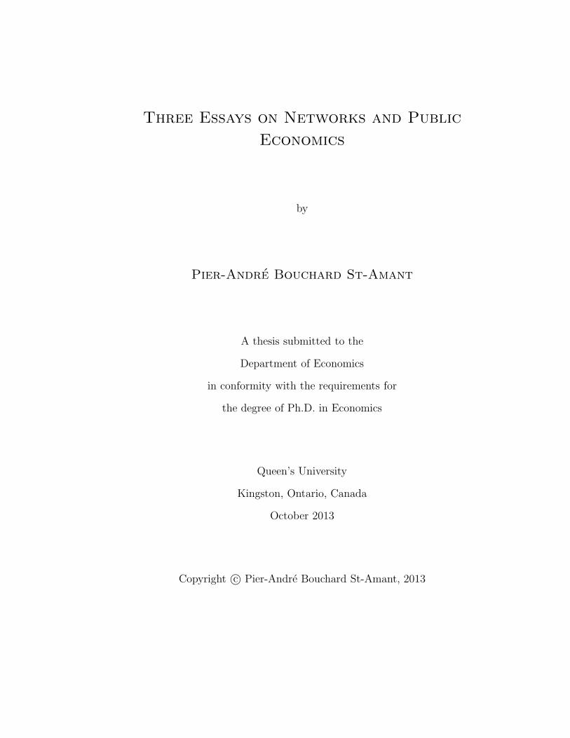
Figure 2.3: The Star and Constrained Star Networks.

Second, any optimal solution s∗j,0 can be written as a discounted sum of signal

selections over time. If we denote kjt as the number of times the signal sj,0 is selected

in time t, the optimal solution solves:

s∗j,0 = p∞∑

t=0

k∗jtβ

t.

What generates value is exposure. Hence, the number of time a signal is carried

over in the next period, as counted by kjt, matters to measure exposure in the next

period. Hence the discounted sum of the number of selections represents the marginal

exposure of a signal sj,0. Setting it equal to the marginal cost yields an optimal

solution.

The third step requires the understanding of a network structure that emerges

naturally in the dynamics of signal selection, namely a constrained star network.

Loosely speaking, a star network has all its nodes attached to a central group of nodes

(see Figure 2.3(a)), the center of the star. In a constrained star, some nodes are not

directly connected to the center because the original network topology prevents them


from doing so. They are however connected to the center through a chain of nodes

(see Figure 2.3(b)). The notion of constrained star is defined formally below:

Definition (Path, Constrained Star Network). A path from i to j is a repetitionless

sequence of directed edges eik1 , ek1k2 , . . . , eknj that connects i to j.

A constrained star network is a graph G(V,E) with the following properties:

1. An hub H: a subset of V such that for any two nodes i, j ∈ H, there exists at

least one directed path from i to j.

2. For any other node i ∈ V \ H, there exists one directed path starting at some

node j ∈ H and going to i.

If a network G(V,E) admits at least one constrained star structure, the average

value of the seed at each node is equal to the discounted value of the selling price p1−β

.

So what matters to find the optimal solution is the spread of the value of initial signals

around this average. This spread is maximized when all the seed is concentrated

amongst a small group of users. When costs are quadratic, the maximization of the

spread is equivalent to maximizing the variance amongst all Nash equilibria.

These key steps are described in the following sections. In section 2.3.3, I show

that an optimal solution must be a Nash equilibrium between the network and the

company. I use the example to show that there are many Nash equilibria. In section

2.3.3 I characterize the law of motion and use it to discuss profits and income func-

tions. I show that profits depend on the spread of the initial signal and the value

of contagion of signals. Since both terms increase when variance increases, the first

component is a sufficient metric to optimize profits.


An Optimal Solution Must Be A Nash equilibrium

The following lemma shows how contagion of signals from one user to another can be

tracked in the model.

Lemma 1 (Path Dependance). Let st+1 = G(st) be the law of motion of the users.

Then, for all i, si,t+1 = sj,0 + cj,t for some j ∈ {0, 1, 2, . . . , |V |} and where cj,t ∈ R is

a path dependent number.

Proof. See appendix A.1.1

This lemma says that the signal chosen by user j at time t is nothing but the

original signal of some other user i plus the sum of perceptions that were added over

time through the path of diffusion from i to j. Hence, at each period, the signal sjt

is a function of one original signal. The following definition uses the result of this

lemma to link the choices made by users in time t to a signal in time t = 0. This

allows a discussion of contagion in terms of marginal income.

Definition (Indicator function, Number of choices). Let 1ijt be the indicator function.

It equals one if user i chose sj,0 at time t and zero otherwise. Furhermore define kjt

by

kjt ≡|V |∑

i=1

1ijt,

that is the number of users who choose signal sj,0 at time t.

If the signal sj,0 has been chosen kjt times in period t, the company can generate

an income of pβt(

kjtsj,0 +∑

i∈{i:1ijt=1} ci,t

)

. So it is important to count the number

of times it has been chosen at each period to establish an optimal signal value.

The next proposition summarizes that any possible solution to the company’s

problem must be a Nash equilibrium.


Proposition 1 (Candidate Solutions). Let S ={

{sjt}∞t=0 ,{

kjt

}∞

t=0

}|V |

j=1be the set of

candidate solutions. Then any s ∈ S must satisfy:

1. st+1 = G(st);

2. kj,0 = 1 ∀j;

3. The seed {sj,0}|V |j=1 induces selections by users such that for all periods and users,

the number of choices for a particular signal is given by kjt;

4. Given these kjt, sj,0 solves:

sj,0 = p

∞∑

t=0

βtkjt ∀j;

5. If the network admits at least one constrained star topology, the average value

of the initial signals it then given by:

1

|V |∑

j∈V

sj,0 =p

1− β.


The Nash equilibrium is summarized in points 3 and 4 of the proposition. Given

that sj,0 is the strategy of the company for user j, it must be that users over the

network chooses that signal kjt times at time t. Now given that users have chosen the

signal j kjt times at time t, sj,0 must account for the marginal contribution pβtkjt at

time t. Summing over all periods yields the marginal income and thus, a candidate

solution.

The fourth item of this proposition makes quite clear what matters in seeding a

node. It is a measure of the discounted social influence of each node. Any solution

has to account for the discounted number of users who will select the information.

The more a source is selected the more it is influent.


We can see this clearly in a node-time diagram. In Figure 2.4, I depict one

possible case of the dynamics4 of the example I previously described (Figure 2.2(b)

and equations 2.1 to 2.4). Each column of nodes represents a user in time while

arrows reflects the contagion of signals through time. At the center of each user is

the initial signal that has been selected by this user. In the picture, the signal s3,0 is

such that it is selected three times by users at each future period while s2,0 is selected

only once every period. This means that k3t = 3 for all t > 0 and k2t = 1 for all

periods. Signals s1,0 and s4,0 are never selected, so k1t = k4t = 0 for all t > 0. This

means that given these kjt, the company must set signals according to:

s1,0 = p, (2.5)

s2,0 = p(1 + β + β2 + β3 + . . . ), (2.6)

s3,0 = p(1 + β3 + β23 + β33 + . . . ), (2.7)

s4,0 = p. (2.8)

The last statement of proposition 1 says that the average value of all signals must

equal the discounted value of the marginal income. This means that all candidate

solutions on a network with at least one constrained star in it have the same average

value in t = 0. Thus, what discriminates the elements in S is the degree of variation

amongst signals given to users.

In the example of Figure 2.2(b), there is more than one solution satisfying the

conditions of proposition 1. The signal s3,0 is chosen at time t = 1 by user 4 only

if s3,0 + 3 > s2,0 + 4. There are thus two cases. The first case leads to the previous

optimal solution. The second case is when s3,0+3 < s2,0+4. In this case, k21 = k31 = 2

and since the network is symmetric, it is true for every subsequent period. For any

4Recall that an arrow represents the selection of a source.


User 1

s1,0

User 2

s2,0

User 3

s3,0

User 4

t = 0s4,0

t = 1s3,0 s3,0 s2,0 s3,0

t = 2s3,0 s2,0 s3,0 s3,0

t = 3s3,0 s3,0 s2,0 s3,0

......

......

...

Figure 2.4: Node-Time Diagram of the Example in Figure 2.2(b)

of these two solutions, users one and four have no influence over other users because

they have no friends who listen to them. This means that their optimal seeding value

remains s∗1,0 = s∗4,0 = p as it is the only solution to these equations. Thus, the two5

5There are actually three solutions on the network. But since it is symmetric, two solutions areidentical, up to a permutation in seeds. By a permutation of the seed at s3,0 with the seed at s2,0in the high variance solution, one gets another solution.


solutions are:

s1,0 = p

s2,0 = p+ 2pβ

1− β

s3,0 = p+ 2pβ

1− β

s4,0 = p

Smallest Variance Equilibrium (example of Figure 2.2(b))

s1,0 = p

s2,0 = p + pβ

1− β

s3,0 = p + 3pβ

1− β

s4,0 = p

Highest Variance Equilibrium (example of Figure 2.2(b))

I will refer to these solutions as the “highest” and “lowest” variance equilibrium.

Notice that s3,0 +3 > s2,0 +3 holds only if (2p+1)β > 1, so this is a candidate equi-

librium that belongs to S if this is true. Otherwise, the smallest variance equilibrium

is unique. In any case, all these candidate solutions are such that∑

si0 =p|V |1−β

since

the network admits at least one constrained star.

If (2p + 1)β < 1, there is only one equilibrium, so it is the optimal solution.

However, if (2p+1)β > 1, which of these equilibria should be picked? Intuitively, the

one with the highest variance yields the highest profits because more value is kept

through the process of replication. But in this equilibrium, there is a loss of value

since information travels on edges of low perceptions (e12 rather than e13). So there

might be a trade-off between the replication process and the gain in perceptions. I

will show later that this is not the case. In order to do so, I first characterize the

conditions of emergence of candidate solutions. Each candidate solution is linked to


a possible constrained star network. Each constrained star network is in turn linked

to the eigenvalues of the law of motion.

On the Dynamics of Signal Selection

So far, I have written very little about the optimal profits. I have also written very

little about the law of motion st+1 = G(st). The law of motion and profits/income are

related as one must first characterize I(0, p), the social value of the network, before

calculating income and profits. I first introduce the main results and then show in

details how to get them.

If the network admits at least one constrained star network, I show that it enters

a periodic regime of period T after a finite transient time t∗. What this means is that

after t∗, the law of motion G can be described by:

si,t+T = si,t + λT ∀t > t∗.

The element λ is defined as the highest average perception over all possible loops of

the network (I describe this in more depth later on). The value T is pinned down by

the greatest common divisor of all cycles with average value λ. This result implies

in turn that users select the same neighbors after a while as they remain the most

valuable.

This pattern of source selection generates a constrained star network. After t∗,

the loop with the highest average fuels all the other users who connects to them. The

pattern of connections for those users, the “branches”, are constrained by the sources

available. Hence, after t∗, highly perceived agents are selected over and over directly

or indirectly.

These results in turn gives a characterization of the profits formulation and the


social value of the network. That value can be interpreted as the value the advertiser

gets for free, without any campaign design from the company. It is the simple action

of users talking about the product.

To prove these results, a bit of investment in mathematics is required. The law of

motion is based on si,t+1 = maxj∈ηi(sjt+ bij) which is non-linear in standard algebra.

However, it is linear in what is called a tropical algebra or a max-plus semiring. If

one defines the addition operator over numbers a and b as the maximum operator

(a⊕ b ≡ max(a, b)) and the multiplication operator over numbers a and b as standard

addition (a⊗ b ≡ a+ b), one then gets the basic operations of a tropical algebra. An

expression like:

si,t+1 = maxj∈ηi

(sjt + bij) + bi, (standard algebra)

becomes

si,t+1 =⊕

j∈ηi

bij ⊗ sij, (inner product in a tropical algebra)

which is nothing but an inner product in this algebra. Hence, if we define a transition

matrix B by the elements [B]ij = bij , the system can be written as st+1 = B ·st, a first

difference linear equation. Thus, one can recover the essential tools of first difference

equations like eigenvector/eigenvalue decomposition.

I introduce with greater details the main structure of linear systems on a tropical

algebra in appendix A.2. Readers looking for a complete and formal treatment should

read the book by Bacelli and coll. [2]. In the body of this article, I present only the

important definitions and theorems to get the results. To begin with, I start by

defining “highest average loops”, that is the notion of critical cycle. Critical cycles

pins down the increase of λ and the length of the periodic regime.


Definition (Critical Cycles). Let C be the set of all cycles on G(V,E). For any cycle

c ∈ C of length |c|, let

ρ(c) ≡∑

eij∈c

bij|c|

be the average value of perceptions and C(G) be the set of all cycles in a network

G(V,E). A cycle cc is critical if

cc ∈ arg maxc∈C(G)

ρ(c).

Denote λ = maxc∈C(G) ρ(c).

This definition assigns a number to all cycles in the network, namely the average

increase of the signal through perceptions over each cycle. The critical cycles are the

loops with the highest average. Notice that by construction, any cycle is an hub.

In Figure 2.2(b), there is only one cycle, that is {e23, e32} with an average value

of 1+12

= 1. Since it is the only cycle, it has the highest average and is thus a critical

cycle.

Critical cycles are important because they contain users who create the highest

consistent increase of the signal through perceptions. Since users choose signals they

like best, they will eventually be influenced by the users in critical cycles, those that

have the highest combination of perceptions.

Now, I will use results on tropical algebras to show the existence of the periodic

regime. I start with the definition of eigenvectors and eigenvalues in the context of

this model and then state the main mathematical result.

Definition (Iterated Law of Motion, Eigenvalues and Eigenvectors). Let st+1 = G(st)

be the law of motion associated with a network G(V,E). Define the iterated law of


motion on G(V,E) by the composition function:

GT (s) ≡ G ◦G . . .G ◦G(s)︸︷︷︸

T times

.

Let furthermore BT · s be its representation on a tropical algebra. An eigenvalue-

eigenvector pair (λ, v) is a solution to the equation:

BT · v = λT ⊗ v,

or in standard algebra:

GT (v) = v + Tλ.

With these definitions in hand, one can show the following:

Theorem 1. For any network G(V,E) which admits at least one constrained star,

then:

1. There exists a transient time t∗ <∞ after which the network enters a periodic

regime of frequency T . T is given by the least common multiple of the length

of all critical cycles while t∗ is no longer than the longest directed path between

any two points;

2. There exists v1, v2, . . . vT eigenvectors such that GT (vi) = vi + Tλ. Each eigen-

vector corresponds to one period;

3. These vectors are formed by the columns of the matrix [B∗]ij ≡ max([BT −

Tλ]ij, [B2T − 2Tλ]ij, [B

3T − 3Tλ]ij, . . . ).

4. In particular, define [v∗]i ≡ max(v1i, v2i, . . . vT i), then v∗ is the unique eigenvec-

tor on G(V,E) :

G(v∗) = v∗ + λ;


Proof. See Bacelli, Cohen, J. Olsder and Quadrat [2]. In particular, section 3.2.4 pp

111-116 for the notion of eigenvectors and section 3.7 pp. 143-151 for the cyclicality

and the finiteness of the transient time.

The most stringent requirement is that there exists at least one cycle in the net-

work. This means that there is a group of users who settle to listen to each other. If

there is no cycle, then any word-of-mouth campaign will end in finite time t∗. In this

case, all kjt = 0 after t∗ and the conditions for proposition 1 remains.

But if there is at least one cycle, the system will enter a periodic regime. The

nodes that have no path connecting them to the cycle will have no long run value, as if

there is no cycle. Hence, they change very little in the analysis. Given the clustering

features of most real networks, having at least one cycle in a network seems like a

weak condition.

In the example of Figure 2.2(b), the only critical cycle has an average value of 1,

so λ = 1. There are only two nodes on this cycle, so T = 2. The eigenvectors are

given by v1 = [3, 0,−∞, 2]′ and v2 = [2,−∞, 0, 3]′. This means that v∗ = [3, 0, 0, 3]′.

In particular, one can check that:

G(vi) = vj + 1 ∀i 6= j, G2(vi) = vi + 2 ∀i,

G(v∗) = v∗ + 1.

The eigenvalue measures the overall increase on the network due to the critical

cycles, while the eigenvectors measures the increases net of λ due to choices made by

users. The interpretation for the components of v∗ = v1 ⊕ v2 is similar: it gives the

maximal increase that will occur over all periods given the selections made by users.

The last proposition allows to find the following results for the optimal solution:


Proposition 2. Let G(V,E) admit at least one constrained star topology and consider

s ∈ S. Then:

1. Any s can be written as:

sj,0 = p

t∗∑

t=0

βtkjt + pβt∗+1

1− βT

T−1∑

u=0

βukj,u,

where kj,u is the number of times signal sj,0 is chosen in the u-th period of the

periodic regime;

2. The income generated by the network is given by:

I(s, p) =1

2

∑

i=0

(si0)2 + pλ

|V |β(1− β)2

+ pβt∗+1

1− βT

T−1∑

u=0

βu∑

i∈V

[Gt∗+u(s0)− s0

]

i

· · ·+ p

t∗∑

t=0

βt∑

i∈V

[Gt(s0)− s0

]

i

3. Denote 0 the zero vector. Then, profits are given by:

Π(s, p) =1

2

∑

i=0

(si0)2 + p

βt∗+1

1− βT

T−1∑

u=0

βu∑

i∈V

[Gt∗+u(s0)− s0 − v∗

]

i. . .

· · ·+ pt∗∑

t=0

βt∑

i∈V

[Gt(s0)− s0 −Gt(0)

]

i.

4. If s′ ∈ S is another candidate solution, then the difference in profits is given by:

∆Π(s, s′, p) ≡ Π(s, p)− Π(s′, p),

=1

2

∑

i=0

[(si0)

2 − (s′i0)2]+ p

βt∗+1

1− βT

T−1∑

u=0

βu∑

i∈V

[Gt∗+u(s0)−Gt∗+u(s′0)

]

i. . .

· · ·+ pt∗∑

t=0

βt∑

i∈V

[Gt(s0)−Gt(s′0)

]

i(2.9)

Proof. See Appendix A.1.3.

The first statement is a simple corollary of the periodic nature of the law of motion.


Since after t∗ the choices becomes periodic, the optimal solution can be written as a

discounted sum of every period.

The second statement characterizes the total value of the network. It states that

the optimal income is the sum of four components. The first term is the income that

stems out of the value of s∗j,0. The second term is the value generated by users on

critical cycles. As these users are those who increase the signal the most repeatedly,

they are those who lead the increase of the signal. Because users look for higher

signals, all of them eventually connect to them through the means (neighborhoods)

they have.

Notice that this income is generated regardless of the chosen solution. This can

be thought as the social value created from the network as users finds out about the

product by themselves. If the highest average cycle λ is positive, this has a positive

value, but nothing prevents from λ to be negative. This depends obviously on spins

and perceptions on the network.

The third term is the value of contagion that is implied by the chosen campaign.

It measures the increase of value from choosing highest valued sources in the periodic

regime. It is thus independent of λ. To see why, imagine that all spins and perceptions

bij + bi are subtracted by λ, the highest average cycle is thus zero (and so is the social

value of the network). However, the marginal changes due to perceptions from one

source to another remains the same. Hence, users still make the same choice of source

over time.

The last term is the value of contagion generated by transitionary dynamics from

(t = 0 to t∗) and has the same interpretation as the third term. It measures the

increase of value from choosing highest valued sources in the transitionary dynamics.


The third statement describes the profits that the company can capture. It has

almost the same interpretation as income. First, the two terms that depends on

the value of perceptions implied by the campaign are now net of the social value

(I(0, p)). In the long run, the effortless campaign generates the vector v∗ at every

period. Second, the component of income implying λ disappears as the advertiser

gets it for “free” if the company performs no campaign.

The formula of the last statement is a simple generalization of the third one: it

compares the value of two equilibria in S.

In the example of Figure 2.2(b), if (2p + 1)β > 1, the highest variance Nash

equilibrium is given by s0 =[

p, p+ p3 β1−β

, p+ p β1−β

, p]′

. Since λ = 1, the social value

is given by p 4β(1−β)2

. Given the solution s0, the network enters the periodic regime with

the state associated with the first eigenvector v1 = [3, 0,−∞, 2] and v2 = [2,−∞, 0, 3]′

in the second period, so the transient time t∗ = 0. Since nodes 2 and 3 are in the

critical cycle, v =[

p+ 3 β1−β

, p+ β1−β

, p+ 3p β1−β

, p+ 3p β1−β

]′

. If the vector 0 is seeded

to the network, the system enters the eigenstate v∗ = [3, 0, 0, 3] after one period and

remains in it forever. One can then calculate profits for the highest variance solution:

Π(s∗, p) = p2 +1

2

(

p+3pβ

1− β

)2

+1

2

(

p+p

(1− β)

)2

︸︷︷︸

Value of the N. eq.

+pβ

1− β

[

2

(

p+3pβ

1− β

)

− 1

]

︸︷︷︸

Value of Contagion

.

(Highest Variance Profits)

With similar calculations, one can find the profits for the low variance equilibrium,

which gives the following difference in profits:

∆Π(s, s′, p) =2p2β2

(1− β)2+

p2β2

(1− β)2− pβ

1− β.

The first term measures the quadratic increase du to an higher dispersion of the seed.

The second term measures the gain of value through contagion. However, this gain


is lowered by the fact that agent one chose a source with a lower perception, which

is measured by the third term.

Notice that the whole sum is positive if (3p + 1)β > 1. Recall that the condition

for the two equilibria to be sustainable is that (2p+ 1)β > 1, so the highest variance

equilibria turns out to be s∗. As the next proposition state, this is not fortuitous.

Proposition 3. Assume G(V,E) admits at least one constrained star and define the

variance on s ∈ S by :

var(s) ≡ var(s0) =1

|V |∑

i

(

s0,i −p

1− β

)2

.

Then, s∗ maximizes the variance on S.


This proposition establishes a complete order on all elements in S. If one candidate

solution has a smaller variance than another, then it cannot be an optimal solution.

In other words, the company has an incentive to steer the network clear of any path

where users share the same signal.

The fact that variance can be used as a metric of optimality pertains to the

specificity of quadratic costs. However, the idea that the company has incentives

to concentrate the value of the seed amongst users pertains to the use of the max

operator from individuals. So this result might change in its form if another cost

function is chosen, but is robust to the choice of the cost function in nature.

The intuition for this last result can be illustrated. Higher signals increase chances

of replication. To illustrate it, assume a complete network where users do not modify

the signals (bij = 0 ∀i, j). In this framework, everybody listens to everybody and

there is no change to signals due to perceptions. In this context, if the company


sends an initial signal of value p1−β− ǫ to all but one user who has p

1−β+(|V | − 1)ǫ, it

is certain that all users will choose this higher signal in the next period: perceptions

are all identical and the signal is higher. So in only one iteration, a value of (|V | −

1)(

p1−β− ǫ)

is lost no matter how small ǫ is. Given these choices, the social network

owner has an interest in focusing on the selected user to increase the value of the signal,

which in turns decrease the value of other signals. This increases the dispersion of

signals across users6.

2.3.4 Network Efficiency

This section explores what happens to the social network structure of information

once the network has entered a periodic regime. In short, it becomes a constrained

star network. The network is constrained because not all users can connect to the hub,

as imposed initially by the neighborhood η of each user. So the periphery consists

of nodes that are to the hub through a chain of users (see Figure 2.5). These paths

are in turn characterized by the sequence of perceptions (bij + bi) that maximizes the

average increase over the length of the path.

The star network structure is an efficient configuration under a vast number of

circumstances (see Jackson ch. 6.3 for a description). Intuitively, this is the most

efficient configuration of the network to maximize the spin from the center to the

edges. Since node all nodes have a connection to the center of the star, the network

can only achieve a constrained version of it.

Proposition 4. Let G(V,E) admit at least one constrained star topology. Then after

the transient time t∗, users on the network generate at least one constrained star

6In this simple argument, one can also see the roots of an algorithm to find the optimal solution.


0 1

2 3 4 56 7 8

910

1113

14 15 1617 18

19

2021 22 2324

2526 27 28 29

30

31

32 33

34

35 36 37 38 3940

41 42

43 44 454647

48 4950

5152 53

54 55

⇓0 1

2 3 4 56 7 8

910

1113

14 15 1617 18

19

2021 22 2324

2526 27 28 29

30

31

32 33

34

35 36 37 38 3940

41 42

43 44 454647

48 4950

5152 53

54 55

Figure 2.5: Networks Splits into Constrained Star Networks


network structure where:

1. All the hubs are a critical cycle;

2. All users that are not in the hub are connected through a path that maximizes

the increase of the signal between the hub and the user.

Proof. See Appendix A.1.5

This means that even if users are not aware of the whole structure of the network,

a structure of spin efficiency emerges. There is a cycle of users that share the most

informative signal and other users attach themselves to this cycle in the way that

maximizes the diffuse such most informative signal. This structure reproduces the

patterns found in the paper by Leskovec, Adamic and Huberman [29]. It finds that

cascades of recommendations are led by a small group of active users (the hub) to a

chain of users (the constrained periphery).

This efficiency result must be interpreted with caution. It means that the networks

organizes itself in a way that it maximizes the diffusion of the most informative signal.

Nothing says, from a normative point of view, whether such signal with respect to a

given product is a good thing. This could, however, serve as a basis of explanation

for market bubble behaviors. I push this idea further in section 2.6.2.

2.4 An Algorithm to Find the Solution

In this section, I present the key elements of an algorithm that computes the solution

in polynomial time.That means that for a given size |V | of the network, the time to

compute the optimal solution is a function of a polynomial in |V |.


The algorithm is a modified version of the greedy algorithm and can be described

in a few steps. Each iteration seeks to seed as much of the total value(

p|V |1−β

)

to each

agent without modifying the selections of users implied by previous iterations. Hence,

the algorithm needs to know what share of the total value remains at each iteration.

It also needs to know an upper bound, the maximal value that untreated users can

have without changing the pattern of selections induced by treated nodes.

1. Initialize the current budget to p |V |1−β

, the upper bound to ∞ and the set of

treated nodes to the empty set.

2. While the set of treated nodes has less than |V | elements:

(a) Inititalize the seed in the following fashion. For all treated nodes, set

their value found in the previous iterations. For untreated nodes, pick one

node and set the seed for this particular node to the value of the current

budget and set to zero to all other untreated nodes. Compute the closest

sustainable Nash equilibrium.

(b) Repeat for all untreated nodes and keep the resulting solution that has

the highest value. Call the node v(i) at the i-th iteration leading to such

solution.

(c) Update the current budget by subtracting the value allocated to v(i). Find

the upper bound such that v(1), v(2), . . . , v(i) will remain unchanged. Set

the current budget to the minimum between this value and the updated

current budget.

(d) Add v(i) to the set of treated nodes.


A formal description of the algorithm can be found in appendix A.4. This algo-

rithm exploits two properties of the model. First, concentration is good. So it seeks

to put as much value as possible in a node at every possible step given that the av-

erage value must be p1−β

. Second, it exploits the fact that the solution must be Nash

equilibrium. Brouwer’s fixed point theorem allows to compute a Nash equilibrium

through the following formula:

h(s0) ≡

∑t∗

t=0 βtk(1, t, s0) +

βt∗+1

1−βT

∑T−1u=0 β

uk(1, u, s0)

...

∑t∗

t=0 βtk(i, t, s0) +

βt∗+1

1−βT

∑T−1u=0 β

uk(i, u, s0)

...

∑t∗

t=0 βtk(|V |, t, s0) + βt∗+1

1−βT

∑T−1u=0 β

uk(|V |, u, s0)

, (2.10)

where k(i, t, s0) returns the number of times a signal i is selected at time t (the vector

of kjts).

I show below that if there exists a mean preserving spread of an existing Nash

equilibrium, it must be that total value of the seed is concentrated further is some

users. This thus establishes a complete lattice on users and one can separate the

problem in finding the most influential user v(1) independently of other solutions.

Then, one can find the second most influential user v(2) given that the value found

for v(1) is part of the solution and so on. The search is thus greatly reduced as there

is a lexicographic value of Nash equilibria.


Lemma 2. Let s, s′ be two Nash equilibria on G(V,E) and assume that s′0 is a mean-

preserving spread of s0 so that :

s′i0 = si0 +∆si0,

with 0 =∑

i∈V

∆si0.

Then, the covariance between the solutions is positive:

∑

i∈V

∆si0si0 > 0.


Hence if a solution concentrates the value in some users, any better solution will

concentrate more value amongst those users.

In order to prove that the steps described above is indeed an algorithm, I need to

define the two key functions that I described informally before. I start by defining

the function that builds a Nash equilibrium.

Definition (Choice Function and Choice Value). Let G(V,E) admit at least one

constrained star with a transient time t∗ and a period T . Define the convex and

compact set

C =

{

s0 : s0 ∈ R|V |, 1 ≤ si0 ≤

|V |1− β

∀i}

,

the choice function k : C × N → N|V | of G by k(i, t, s0) ≡ kit and the Choice Value

function h : C → C by equation 2.10.

This allows to show that 2.10 has a fixed point:

Proposition 5 (Fixed Point of Equation 2.10). Under the same conditions as in the

last definition, the function h:


1. Admits a fixed point s0;

2. Is a contraction.


The intuition that h is a contraction can be seen in Figure 2.6. That Figure

depicts the decision of a user at some given time. This decision is visualized in the

numbers kit. On the horizontal axis, there is the current guess made by the company

about the number of selections kit. These guess forms the actual signals si0 and given

this signal, the user must decide which signal to choose. The solid line represents

his decision rule (max(sit + cmi, sjt+ cmj)) and the vertical axis represents the actual

choice k′it of the user given the current signals.

If the current kit is too low, other signals are higher and it does not affect the

decision, that is the flatline portion of the solid line. If however kit is high enough,

the signal is selected and leads to an increase of kit. Thus, the kink of the solid line

represents the threshold point at which the user change his mind.

In Panel 2.6(a), the current guess kit is too high since the it does not induce

the user to deliver the selection guessed in the seed. Hence, the signal must be

adjusted downward to satisfy first order conditions. This is repeated until k′jt equals

the selection, the point where the 45 degree line meets the solid line.

Conversely, Panel 2.6(a) shows what happens when the signal is too low. In this

case, the user i is more influential than what the current seed assumes and thus the

signal must be increased. If the signal is high enough the user making the decision

becomes the unique source and all his friends listen to him. In this case the value

kit equals kmax in the picture and the fixed point is in the top corner of the picture.

Since the function h is a contraction, I can use it to find Nash Equilibra.


kmax

kmaxkjtk′jt←

(a) The Signal Is Too High

kmax

kmaxk′jtkjt→

(b) The Signal Is Too Low

Figure 2.6: The Function h is A Contraction

In the next proposition, I show that the code stops in finite time. I also show that

the execution time is of an order of |V |5(t∗ + T ).


Proposition 6 (Execution Time). Consider the algorithm described in the previous

pages (formally described in appendix A.4) on a graph G(V,E). Let t∗, T be respec-

tively the transient time and the period. Then:

1. Its execution time is finite;

2. Its execution time is at most of O(|V |5(t∗ + T )) for an exact solution.


2.5 Applications

In this section, I use the model to answer four practical questions. I start with a

market valuation for Facebook. Second, I discuss how the model relates to current

rules of thumb in network valuation. Third, I show how β influences the company’s

optimal strategy. Finally, I discuss the valuation of a single user.

2.5.1 On the Market Value of Facebook

The previous sections have defined what a social network sells and how it can be

exploited to derive some value. So what remains is to use a model of market equilib-

rium.

I do this by assuming that Facebook is a monopoly and that its sole source of

revenue is selling word-of-mouth advertising. As for the sole source of income, other

sources could be included in the description below by simple addition of new terms.

This is thus done for simplicity.

I assume there is a demand function D(p) that represents the demand of in-

terested buyers of a word-of-mouth marketing campaign. The demand function is


differentiable and negatively sloped in p. The price of the campaign would thus solve:

p∗ = argmaxp

D(p)Π(s∗(p), p).

This function admits an optimum7 p∗, yielding profits that can then be divided

amongst shareholders.

2.5.2 Broad or Targeted Campaigns?

Should any company aiming for word-of-mouth target each user equally or should it

focus on one user and give it all the initial information? This paper says that users

should receive more importance by the company when they tend to be selected more

by other users. So a user’s influence is measured as the discounted value of direct and

indirect listeners they have.

This means that the way time is discounted has an impact on the optimal solution.

If β is close to zero, advertisers prefer fast, direct advertising and do not want to wait

for messages to diffuse through a social network. So one can see that when β=0,

the optimal solution is the average solution for all users and the variance is zero.

The average solution is the only Nash equilibrium, so it is the variance maximizing

solution. Everybody is targeted equally with the signal si = p, regardless of the

long-run influence. This is, in some sense, standard advertising.

However, when β approaches one, it is the complete opposite. Notice that in this

case, there is at least one original signal that remains in the network after some given

time t∗. For the sake of discussion, assume it is the only signal that remains. In this

7To see this, notice that profits are increasing in variance and variance is increasing with theprice. Hence, profits are increasing in price. One can easily show that profits are bounded and therethus exists at least one p∗ in [0, pmax] where pmax is defined as D(pmax) = 0.


case, the first-order condition for that signal commands that the signal has the form:

sj,0 = pt∗−1∑

t=0

βtkjt + pβt∗

1− β|V |.

As β goes to one, the value of the last term gets closer and closer to infinity, while the

value of all other signals remains constant. So the relative importance of this signal

becomes infinite. Relatively speaking, all the initial signaling resources are focused

on one user and the social network lets users build the spin.

To sum up, a concentrated signal is a good strategy for a patient company, while

it is a poor strategy for a company in a rush. Impatience comes at a price of less

exposure over the network and thus, less income and profits.

2.5.3 On Rules of Thumb For Network Valuation

There are two current rules of thumb used by market analysts to evaluate networks,

namely Metcalfe’s Law and Zipf’s law (see [46] for a discussion). Metcalfe’s law

assumes that the value of a network is based on the potential number of links in the

network. So for n users, its value should be of an order of n2. Zipf’s law however

assumes that the value of a network should be of n logn.

In the model above, the profits inherit the properties of the cost structure. This

is so because the optimal value of signals is bounded by a linear function of users.

As such, the profits are bounded by a function that depends on the cost structure. If

costs are quadratic, as it is the case in this paper, there is grounds for Metcalfe’s law.

However, if costs were exponential, Zipf’s law could be recovered as an approximation.

Thus, the structure of the cost function seems important to find the correct rule of

thumb when it comes to word-of-mouth networks. As income is bounded by a linear

function of the users, it seems hard to reconcile theses rules without a look at costs.


2.5.4 What is The Value of A Node?

Imagine the following situation. Before the beginning of an advertising campaign, a

user leaves the social network or willingly decides to stay out of the social network

during the campaign. Although this can be computed using the profits difference

equation in proposition 3, some broad intuitions can be discussed.

There are three possible types of losses that depends on the importance of the

user in the network.

First, the loss due to the disconnection of some users to the hub of the constrained

star. As these users become disconnected from the main source of exchanges, their

long run value vanishes. So if there are n users of that sort, the loss of profits is at

least n2

βt∗p2

(1−β)2. As there is at least one user leaving, this loss is never zero.

Second, there are some additional losses if the user leaving is highly regarded by

others. Since the user leaves, these users must select another source. This changes

the income through the term∑∞

t=1 βt∑

j∈V kjt(bij + bi + cj,t−1) and thus decreases

profits. Conversely, if an agent with low perceptions from others leaves, these losses

are minimal since users do not listen to him.

Third, if the user leaving is on a critical cycle, it can disconnect a lot of users

from an hub as it vanishes. The magnitude of the losses depends on how users will

reorganize themselves around another hub (if any). If there is no hub at all, then all

the long run value of the network that comes from the periodic regime is lost.


2.6 Some Alternative Specifications of Users’ Be-

haviors

In this section, I explore a different class of behavior of agents, namely what happens

if users mix signals to form a new one. I discuss briefly what the first-order condi-

tions look like in that context. I also discuss briefly what happens when perceptions

fluctuate over time. I show how this can be used to model business cycles.

2.6.1 Signal Mixing

Here, I explore what happens when users mix the signals they receive. Instead of

picking the signal they like best, I assume that they adopt a more prudent behavior

and use some form of averaging across signals.

Definition (Users (modified)). A user{

ηi, {bij}j∈ηi , f}

forms a new signal according

to their perceptions of neighbors and the signal they get according to the function:

si,t+1 =

1

|ηi|∑

j∈ηj

bijsrjt

1/r

,

where r is a measure of importance to the highest signal.

Notice that the modification of the signal according to perceptions depends now

on the signal, as perceptions are multiplicative (through bij). The greatest advantage

of this change is that perceptions can now change the sign of the signal. If aij is

greater than one, it amplifies the signal while it is the opposite if it is smaller but

positive. If this number is negative, it can also mean the two neighbors disagree on

the informativeness of the signal. For instance, one might think a political party has

a positive value while another one thinks it has a negative value.


i

a

b

c

1

2

3

2

(a) r = 1

i

a

b

c

1

2

3

2.47

(b) r = 5

i

a

b

c

1

2

3

2.93

(c) r = 50

i

a

b

c

1

2

3

3

(d) r → ∞(max behav-ior)

Figure 2.7: Weight of Sources In Signal Formation For user i Given Values of r.

The parameter r is a measure of excitement for the highest valued signal. No-

tice that if r goes to infinity and bij = 1, ∀i, j, the behavior boils down to si,t+1 =

maxj∈ηi (sijt), which is the essence of the previous model. Users pick the highest sig-

nal. If r = 1, we have a standard linear model (as in the DeGroot Model) and users

average. In Figure 2.7, I illustrate how r influences the selection of the signal mix

using shades of gray. The higher is r, the more the highest signal comes in the mix.

Although there might be some grounds to model agents with this behavior, there

are two dissatisfying things about it. First, users do not choose anything dynamically:

they always average. Second, as all sources remain always employed, the constrained

star structure is lost and the model thus loses its empirical match.

Nonetheless, I discuss below what first-order conditions looks like and provide one

interesting example based on the fact that users can now disagree on the direction

the signal should go.

The following definition introduces the adjacency matrix, which allows to use the

standard inner product and linear algebra.

Definition (Adjacency Matrix, Vector of Spins). Let the adjacency matrix B ∈ R|V |2


be:

[Bij ] ≡

bij if j ∈ ηi,

0 otherwise.

Recall that a square matrix B can be decomposed in an unit-eigenvector/eigenvalue

of the form A = V ΛV −1 matrix form and thus, Bt = V ΛtV −1.

That decomposition separates the dispersion effect of the signal (through V ) from

the amplification effect of the signal (through Λ). The norm of a unit-eigenvector

equals one so the interpretation of one of its component is the share of dispersion of

the signal to a given user. For instance, if the element vij is equal to√0.5, this can

be interpreted as if 50% of the signal in j is shared to i. The value λi, the ith element

on the diagonal of the matrix of eigenvalues, has also a clear meaning: it tells how

much of the signal passing through i is amplified by perceptions, at each period of

the model. As the company is interested only in amplification, this is the element of

interest. I present below the characteristics of the optimal solution.

Proposition 7. Given the current behavior, the optimal solution solves:

s∗i0 = p

∞∑

t=0

βt

|V |∑

j=1

[Bt]ji

(s∗i,0s∗j,t+1

)r−1

,

= p

∞∑

t=0

βt

|V |∑

j=1

[ViΛ

tV −1j

](

s∗i,0s∗j,t+1

)r−1

.

In particular, if r = 1, the solution solves:

s∗0 = pV DV −1ı

where ı is a vector of ones and D =∑∞

t=0 βtΛt



The structure of the first-order condition captures the amplification value of users

in the network at each period in time. This amplification is weighted by the share of

si0 that goes in j at time t+ 1. This weight is also modified by r − 1, to account for

the tastes for the highest-valued signal.

When r = 1, the solution has a compact form. The total amplification is given

by the adjacency matrix V ′DV −1 where D is a diagonal matrix with elements 11−βλi

,

that is the total discounted value of amplification for a given user i.

An Example: Two Opposing Parties

In this section, I use the fact that spin can change the sign of the signal to show that

reverse-psychology can be an effective word-of-mouth strategy. Consider the reduced

form of members of two political parties. One party seeks the best message given

that other members will always say the opposite. The network structure can then be

characterized by the adjacency matrix:

B =

0 1

−1 0

,

with b = 0. I show in Appendix A.3, that if r− 1 is odd, the optimal solution solves:

(s∗2,0)r−1 =

p

1− β5

[1− β + β2 + β3 + β4

](s∗1,0)

r−2,

(s∗1,0)r−1 =

p

1− β5

[−1 − β − β2 − β3 + β4

](s∗2,0)

r−2,

and notice that if β is small, this can lead to a negative value for s∗1,0. This means

that reverse-psychology, initial values saying the opposite of what the party believes

in, can be part of an effective word-of-mouth strategy if there are users who share the

opposite of the message they receive.


2.6.2 A Network Foundation of Business Cycles

In this section, I illustrate that the company has incentives to deviate from a path

where users agree on the signal over time. I do this by modifying the model to allow

users to modify their net perceptions bij based on the past values of the signal they

received. I do this in a simple fashion by assuming users react to a simple quadratic

formulation of their preferences for information they receive and information they

prefer (measured by φ):

si,t+1 = maxj∈ηi

(sjt + bij(s)),

bij(s) = argminaij−(1− θ)

(sjt + bij(s)− φ)2

2− θ

(sjt + bij(s)− sj,t−1)2

2,

= (1− θ)φ+ θsj,t−1 − sjt

⇒ si,t+1 = (1− θ)φ+ θmaxj∈ηi

(sj,t−1)

This modification of perceptions is simple to interpret. The user tries to balance the

perceptions about each source between what he thinks is the right value for the signal

and by how much the signal has changed from this source over time. Here, there is

the assumption that if the signal changes over time, the source j is trying to oversell

and thus, the perceptions will decrease the signal.

As all users have the same intrinsic preference for information, φ, it should be

intuitive that the long-run value of the signal would converge to it. I characterize this

equilibrium below:

Definition (Perfect Neighborhood Foresight). A Perfect Neighbor Foresight behavior

is when aij(st) = 0 ∀i, j.

In words, a perfect neighbor foresight is when all users receive the same signal and

they think this value is correct. They thus form neutral perceptions about each user.


Proposition 8 (Perfect Neighborhood Foresight Regime). If users have a perfect

neighborhood foresight, then:

1. The social network value is 0 (λ = 0);

2. Users are indifferent about their sources of information;

3. The signal shared over the network is φ for all users.


In a perfect neighborhood foresight regime, the structure of the network has no

value as everybody agrees and shares the same signal over and over. Hence, any

source is as good as others.

It should be however intuitive that, this is suboptimal from the company’s per-

spective. If one user has a signal higher than others, some neighbors will choose it

and this will increase the marketable value of the signal. In the long run, however, the

signal will come back to φ, in a perfect neighborhood foresight regime. When there

is no perfect neighbor foresight, there is a viral spin in the network and the principal

can exploit it to derive some value. I formalize this in the following proposition.

Proposition 9 (Perfect Neighbor Foresight Regime Suboptimality). If θ 6= 1, a

Perfect Neighbor Foresight Equilibrium is suboptimal from the company’s perspective.

Proof. It is sufficient to notice that if θ 6= 1, there exists a mean preserving spread of

[φ, . . . , φ]′ that can increase the company’s profits.

In other words, if there is some periodic regime where users agree on the signal

to be shared over the network, the company has incentives to change the value of the


signal to actually generate some cycle that will slowly converge back to the original

equilibrium.

In this example, the change in perceptions is deliberately made simple to show

that the variance maximizing component applies to changes in perceptions. However,

some additions would be needed to make this interesting in terms of business cycles.

So instead of generic signals, users could share valuations about the future through

a strictly convex valuation function Vit(k). They would thus seek the best valuation

given the ones they received from their neighbors trough the process:

Vi,t+1 = maxu(k)+Vj,t(k)∈ηi

u(k(j)∗) + βVj,t(k(j)∗)

k∗j ≡ argmax

ku(k) + βVjt(k).

Hence, what users would send are valuation functions (what they think is the best

way to value an asset). In this case, the simple fact that valuations take time to travel

from one agent to another could generate substantial persistence over the aggregate

economy with simple technological shocks.

2.7 Conclusion

In this chapter, I characterize the optimal solution to a word-of-mouth campaign over

a social network. I do so in an environment where a company can seed information

to users who choose afterwards which information they share with their neighbors.

The profit maximizing solution is a unique Nash equilibrium. I show that amongst

all sustainable Nash equilibria, the optimal one maximizes concentration amongst a

small set of users. Hence, concentration of the signal to a small group of users is good

as the network replicates the information for free.


I also show that after a transition period, the word-of-mouth dynamics enters a

periodic regime. Users on the network listen to the same sources over and over. Their

uncoordinated actions are such that the social network becomes the most efficient

structure to carry information given the possible sources available to users, namely

a constrained star structure. The perceptions amongst users is a key element in

determining who is at the center of this star of influence.

I present an algorithm that can compute the optimal solution in polynomial time

on any network topology. Hence the model provides a tractable solution on large

scale networks.

In particular, I show how this model can be used to price Facebook. If analysts

measure the value of a social network company like Facebook solely on the value of

direct advertising, they underestimate the value of the information the company has

as it simply neglects the value of word-of-mouth.

Chapter 3

Some Notions of Public Economics

on Networks

3.1 Introduction

Word-of-mouth communication is a topic widely discussed when it comes the eco-

nomics of social networks. Some papers cover the endogenous formation of com-

munications networks (Galeotti, Ghiglino & Squintani 2009), others are interested

in harnessing the process from a marketing or sales perspective (Godes & Mayzlin,

2001), while others examine the impact of word-of-mouth on the behavior of agents

on the network (Schiraldi & Liu, 2010). However, very little is said on contagion from

the standpoint of public economics.

In this chapter, I use the same model of word-of-mouth communication I developed

in the previous chapter to discuss network spillovers and the notion of social value of

a network. I show how these concepts come in play in word-of-mouth communication

and sometimes fuel the demand for such type of advertising. The key driver is that

60

CHAPTER 3. SOME NOTIONS OF PUBLIC ECONOMICS ON NETWORKS 61

ideas and discussions are non-rivalrous. If an idea is disseminated to a neighborhood

of friends, nothing prevents these friends to reproduce it at will. Since this effort of

reproduction is in essence the action of the network agents, it comes for free for an

advertiser. As such, a network is a technology that allows for the reproduction of

ideas for free.

Anyone with a Twitter or Facebook account can see this process of information

reproduction at work. Topics range from the latest Justin Bieber song to information

about earthquakes (Sakaki, Okazaki & Matsuo, 2010). For instance, roughly 6000

Justin Bieber fans showed-up on a rumor of a concert spread on twitter (see Ryland

2012). In short, seeding one idea on the network might go a long way through a

process of replication: that is, in essence, the contagion spillover.

The natural idea, from a sales point of view, is to try to exploit this phenomenon

to increase sales. For instance, a company might want to target a group of users

and let them evaluate a product to generate some word-of-mouth advertising. By

selecting the right group, the company can use the network to generate a cascade of

positive recommendations that can increase sales. This cascade of adoption might

be caused by herding (as in Banerjee, 1992), by an informative signal about the

quality of the product (Cambell 2005, Vettas 1997) or simply be the result of truthful

communication (Galeotti and Goyal, 2009). The consistent feature of these models

is that regardless of the motives of the agents on the network, or their behavior

(Bayesian updating, randomly talking, or being fooled), they do communicate with

each other. If what drives this communication is known to the company, it can be

exploited to increase profits. The company, however, profits from such communication

for free, and this is where the free rider problem occurs. I show below under which


conditions this problem is important and how it might be solved.

If conversations between agents influence how consumers evaluate or perceive a

product of the company, the company will try to exploit these perceptions as well.

In this case, the process is not only about disseminating an idea, but also about

ensuring the right conversations occur to generate a positive value. However, agents

will discuss ideas even if the company performs no action. The conversation might be

different in nature, but it can be taken as granted that some conversation happens.

Such communication has some value and is, in essence, the social value generated by

the network. Because this exchange of information does not depend on the actions

of the company, it cannot be captured in any fashion. If the discussion is about the

quality of the company’s product, this conversation has certainly some value.

In section 3.2, I discuss the existing literature on network externalities. In section

3.3, I present again the model of word-of-mouth communication over a social net-

work. In sections 3.4 and 3.5, I exploit the model to discuss its implications from a

standpoint of externalities and social value. A brief conclusion follows.

3.2 Literature

To my knowledge, there are no academic articles on the social value of word-of-mouth

communication, nor on the externalities it induces. Some of the academic articles

dealing with network externalities refer to the adoption of a technology (see Katz &

Shapiro, 1985 or Farrell & Saloner for an exposition). This area of literature focuses

on the adoption of a product, where the value of the product depends on the number

of people using it. Such articles are however of little help in the context of word

of mouth because the externality in word-of-mouth is a consequence of discussion


rather than the value of the product. The latter can have a value independent of the

number of adopters but still lead to word-of-mouth communication. In the context

of communication, the contagion effect stems from non-rivalry1 of ideas rather than

the adoption of the idea itself.

However, there are parallels to be made between word-of-mouth communication

and the congestion literature (see Kelly, 2008 for a good introduction). In discussing

about a product, agents on a network let the information produced circulate for free.

As such, companies profit from this information flow although they bear no cost in

the process of link formation. Such problem of flow has been studied in the design of

information network or roads. In such cases, the externality is negative: an increase

in the flow (traffic) leads to longer waiting times. The standard approach to address

this externality is to introduce a toll, which influences road users to take the socially

optimal route.

In the context of word-of-mouth communication, the externality is positive if the

product being discussed is valuable: a firm can profit from the process of link creation

between agents on a network to generate a contagion of ideas, or spillovers. Hence,

the externality is different in nature. The idea of tolls can however still be applied to

show how agents can address the free rider problem. This is discussed further below.

1A product is non-rival if its consumption does not prevent somebody else from consuming it aswell. An idea has such a property.


3.3 Model

The Network

This section contains the same model description as in chapter two. Readers can

easily skip this section if they read the previous chapter.

There is a directed network G(V,E) with |V | agents linked together by a set of

|E| directed edges. A particular agent is denoted by an index i ∈ V , while a link

between agents i, j ∈ V is denoted by eij. Since edges are directed, eij represents

the direction of information traveling from j → i. An example is provided in Figure

3.1. The set V = {0, 1, 2, 3, 4, 5, 6} contains seven agents linked by the set of edges

E = {e01, e20, e50, e30, e13, e41, e52, e53, e36, e46, e65}.

This network topology is assumed to be fixed and the outcome of a network

formation process. Various economic models can explain link formation. Some assume

the formation is a consequence of random draws of a given distribution (see the Erdos-

Renyi framework in Jackson, 2009) or a random rewiring of edges of a known network

structure (see Watts and Strogratz, 1998). There are other processes of link formation

based on the allocation of scarce resources in building costly links between agents.

These allocations might be based on a trade-off between personal biases on the state of

the world and the willingness to learn the truth (Galeotti, Ghiglino & Squintani 2009),

or homophily, the tendency for people with similar preferences to be linked together

(Boucher, 2012). Whatever the reason for the form of the network, it is taken as

granted. For the discussion about the externality, it will be useful to assume that link

formation is costly. This can be thought of as the cost to maintain a relationship or

the additional time required to search through a larger set of information.


0 1

2 3 4

5 6

e41

e65

e16

e36

e13

e53

e50

e01

e46

e20e30

e52

Figure 3.1: An Example of A Network

As in the previous chapter, a convenient definition is the notion of the neighbor-

hood of sources of an agent i: ηi. This represents the set of agents from which agent

i can choose to listen to. For example, in Figure 3.1, η1 = {3, 4, 6} since agent 1 has

agents 3, 4 and 6 as sources of information. Agents exchange a signal sit ∈ R on the

network. This signal can take on various meanings: it can represent the quality of a

product, the level of (dis)utility of a message or simply a truthful message about the

state of the world. In all cases, the signal has some value to the agents and to the

company. I give some examples below. This signal might change in time and might

be different from one agent to another. I will denote st ∈ R|V | the vector of signals

distributed by each agent at time t.

3.3.1 The Agents

The next step is to define the behavior of agents regarding the information they have.

Agents are mathematically modeled as three objects: a neighborhood ηi, a set of


personal perceptions bji ∈ R, or biases, and a choice function f : {sj : j ∈ ηi} → s∗j .

The notion of neighborhood has already been discussed: these are the possible sources

of information for a given agent. When these are specified for every agent, the network

structure is fully known. The notion of personal perception pertains to how agent

i values information received from agent j. The higher the value of bji, the more

highly agent i thinks of agent j. One way to think of this is personal preferences

over sources. These numbers could change over time, as with a dynamic reputation

function, but I hold them fixed for simplicity. The choice function represents how

an agent will choose a source of information given its perceptions about other agents

and the signals it receives. In this chapter, I will use the following model of agents :

sit+1 = maxj∈ηi

(sjt + bij) (3.1)

The motivation for this choice stems from numerous examples:

1. Agents learn about the quality of a product only from their neighbors (as in

Campbell, 2012). Such quality is uncertain and can be high or low. They have

a unit demand for it when the quality is high and no demand for it when it

is low. Neighbors can observe the quality of the product when someone in the

neighborhood has bought it. Hence, the vector of signals can be thought of as

a binary vector where each element sit is either one or zero. When the value

is one, the signal means “this Neighbor conveys information: the product is of

high quality,” while when it is zero it means “this Neighbor does not convey

information: it has not bought the product.” In this context, the signalling

process sit+1 = maxj∈ηi(sjt + 0) represents the evolution of the beliefs (and the

demand) about the product over time.


2. The information can be thought as a vector v drawn from a vector space of

concepts. These concepts might be “liberty” and “equality” (a two-dimensional

vector space) and a particular vector represents a level of support for those

concepts. Agents have some given preferences v over those concepts (e.g. what

they believes the right level of liberty and equality) and they weight each concept

according to a diagonal matrix W , each element of the diagonal being a weight

for a concept. The distance function (v − v)′W (v − v) represents a measure

of homophily, or the distance between the message and what the agent prefers

(see Currarini, Jackson & Pin for further discussion on homophily). Hence, an

agent chooses its messages based on sit+1 = maxj∈ηi(−(vj − v)′W (vj − v)+ bij).

That is, they choose the message that is the closest to their own preferences,

given the bias they have for individuals (bij).

3. The information can simply be the perceived quality of information. Hence, sjt

represents the degree of information communicated by agent j and bij represents

the correction agent i applies to agent j’s signal. Once the signal is corrected for

perceptions, agent i sends his own most informative signal: sit+1 = maxj∈ηi(sjt+

bij).

This behavior is sufficient to discuss the economic nature of word-of-mouth com-

munication over a network. There is also some practical reasons for choosing this

functional form.

First, it is tractable on large-scale networks. Social networks are, by design, large.

Facebook has 900 million users, Twitter has 500 million users, and both are growing.

The number of links between these agents is much larger. Although companies or

scientists might be interested in subsets of these networks, they still represent large


objects. Thus, the models used to represent them must be tractable to provide

meaningful answers to practitioners. The model above can be described as a linear

system, very similar to the linear system of equations Bst = st+1 in what is called

a tropical algebra (or max-plus semirings). The solution can thus be found while

avoiding the curse of dimensionality (as detailed in the previous chapter).

Second, the functional form maxi∈ηj (sit + bji) can be ported directly in an econo-

metric setup. The numbers bij can be thought as a reduced form of a sum of char-

acteristics (Xiβ) and a type I extreme error term. This representation then leads

to logistic regressions. The model thus has a probabilistic counterpart that can be

estimated.

All of the examples above share the same constraint: information only flows

through the network structure. In other words, agents are myopic; an agent can-

not get more information than what his sources tell him. In the discussion on ex-

ternalities, I will show that this assumption is critical for the firm to “free-ride” on

the network structure. If agents are able to understand how critical they are to the

spillover effect, they can solve the free rider problem by forming coalitions. This

would, however, require a knowledge of the network structure.

3.3.2 The Company

There is one company that seeks to have information distributed about its product. It

derives value from the fact that consumers are informed by word of mouth. I assume

the company discounts time at the rate β ∈ [0, 1), meaning that messages received

earlier are better. Finally, I assume that the number of periods T is large enough to

let the information reach all agents on the network. For simplicity, I assume that the


number of periods is infinite, although this assumption does not affect the discussion.

Hence, the company values :

I(s0) = p

∞∑

t=0

βt∑

i∈V

sit, (3.2)

where p is some exogenous price representing the market value for word-of-mouth

exposure. This formula captures, in essence, the value derived from the word-of-

mouth discussion about the company’s product. For instance, the company could

value h(sit) where h is some probability distribution of buying, given the signal.

However, the main idea is embodied in I: more information is better, and sooner

is better. This assumes that the information reveals something positive about the

product. As noted by Goyal and Galeotti (2009), if agents perceive the product to

be of poor quality, communication is harmful from the firm’s standpoint. So it is

assumed throughout the chapter that signals convey positive information about a

product.

The firm prefers word-of-mouth advertising to standard advertising because in-

formation that comes from acquaintances has more impact than direct advertising

(Bond et al., 2012). Hence, it seeks to “seed” its advertising message only once, to

a particular group of users on the network, and allow word-of-mouth communication

to disseminate its message further. The firm can choose the seed s0 from a com-

pact strategy space S. For each s0 ∈ S, the company must pay a cost c(s0). This

cost could represent what has to be paid to convince the seeded user to disseminate

the information, or simply the cost of producing the signal. Thus, the firm seeks to


maximize:

s∗0 = argmaxs0∈S

I(s0)− c(s0)

s.t.sit+1 = maxj∈ηi

(sjt + bij) ∀i ∈ V (3.3)

Hence, the firm seeks to maximize exposure given the reaction function of agents.

To stick with the examples above, this problem might represent:

1. A firm that sells a product of good quality that wants to get the word out

through word of mouth. It must use a “money burning” signal to seed some

initial agents on the network while other agents learn quality through their

neighbors. The strategy space is the set of binary vectors with only k ≤ |V |

seeds in it. The cost of any vector is the sum of its components.

2. A political party that seeks to design a popular message with the name of its

candidate in it. It thus seeks the optimal vector v∗ that will maximize diffusion

given the homophilic preferences of agents. The cost of producing this vector

could be linear in the distance to zero: c(s0) = v′v and the strategy space is

defined implicitly as any v∗ such that profits are non-negative.

3. A firm wants to exploit the perceptions of agents on the network to spin the

perceived quality of a product. It might also seek herding to increase sales. The

cost of producing this signal is quadratic in quality(

c(s0) =∑

i∈Vs2i02

)

and the

strategy space is defined implicitly by the set of vectors with positive profits.

The following statement can then be proven:

Theorem 2. Given a graph G(V,E) and the behavior of agents described in (3.1),

then (3.3) admits at least one optimal solution s∗0(G).


Proof. It is sufficient to notice that I(s0) is continuous in s0 and that S is a compact

set. It therefore has at least one maximum.

In the next sections, I will work with s∗0(G) and I(s∗0(G)) to discuss the relevant

concepts.

In this chapter, I leave aside all the technical considerations to find this solution.

For instance, the first example is known to be the set-covering problem (see Cormen,

2009), which is cursed with dimensionality (NP-hard). For a generic value of k, it is

intractable on large-scale networks2.

3.4 The Contagion Spillovers

3.4.1 The Baseline Case

In this section, I assume that the personal perceptions about other agents (bij) are

equal to zero. As I am more interested in explaining the spillover effect and the exter-

nalities rather than a particular form of solution, I proceed without these perceptions

to simplify the exposition. Much of the analysis remains the same when this is not

the case.

As a baseline, I first use the case where E = ∅. In this case, there is no word-of-

mouth discussion at all on the network, as agents are isolated. In this case, the firm’s

decision is quite simple: it will invest in seeding a node if it can derive some profit

out of this note (if si > c(si) for some si ∈ S). If agents are identical, this condition

will be the only one. This leads to the following lemma:

2It is, however, tractable when k = 1, which is the optimal solution to the problem if β is “closeenough” to one.


Lemma 3. If E = ∅, the company seeds the network only if si > c(si) for any agent.

As there is no transmission of the signal over the network, this can be thought of

as the company informing a consumer directly about the product. As the company

pays all costs of seeding, the firm bears the whole cost of advertising. There is little

to discuss about this case, but I use it as a benchmark in the following section.

3.4.2 Word-of-Mouth Externalities and Spillovers

When E 6= ∅, the company can exploit the network structure to increase profits. If

producing links is costless to agents, the increase in profits is done at no expense.

Hence, all the costs of producing the signal is captured by the firm and the additional

profits over the benchmark case are a result of a better technology (a spillover).

However, if producing links is costly to agents, the firm profits from these links at the

expense of those who paid for it. There is a free rider problem.

To discuss this formally, I start by defining how the solution can be expressed in

terms of choices of agents:

Definition (Choices). Let kjt ∈ N denote the number of times the signal s∗j,0 is chosen

as the optimal signal by agents at time t, given their reaction function f . Then, for

any signal s∗j,0, the value generated is given by:

I(s∗j0) = p

∞∑

t=0

βtkjts∗j,0 ∀j.

The optimal solution thus accounts for the discounted number of times each seed

j is being selected. In the baseline case, the signal is selected only once in time t = 0

and never again, since there is no network. But when the network has some edges, it

takes different values in time t > 0. What this shows is that there are now spillovers


associated with the same seed and there is thus some latitude in increasing profits. I

formalize this idea in the proposition below:

Proposition 10 (Profits non-decreasing in links). Let G(V,E) be a graph with its

associated profits Π(s∗0(G)) and consider G′(V ′, E ′) such that V ′ = V,E ⊂ E ′. Then,

Π(s∗0(G′)) ≥ Π(s∗0(G)).

Proof. It is sufficient to notice that Π(s∗0(G)) is still available under G′ and thus,

adding links can only have a non-decreasing effect on the optimum.

This proposition simply states that the company can increase its reach when there

are more links for word-of-mouth discussion. The seed of one agent has a spillover

effect from the agent to some neighbors who choose his signal and thus, increases

exposure.

There is actually more that can be said if one additional assumption is made on

the network topology. If one assumes that there is at least one cycle3 on the network,

then some signals never vanishes and over time all the branches connected to this

cycle share the signals on the cycle. I call that structure a constrained star network.

Hence, if a network can be partitioned in a sub-network containing constrained stars,

the value of the signal never vanishes. Since the max operator ensures that signals are

strictly increasing at any period, one can rewrite the Income in the following fashion:

I(s∗0) = p∑

i∈V

s∗i0

︸︷︷︸

Value of the seed

+ pβ

1− β

∑

i∈V

s∗i0

︸︷︷︸

Long-run value of the seed

+ p∞∑

t=0

βt∑

j∈V

(kjt − 1)s∗j,0

︸︷︷︸

Value of non-rivalry

(3.4)

The first term is simply the value of the seed. The second term measures the value

of the long-run value of the seed. The interpretation is that the firm would get this

3A cycle is a repetitionless path of edges whose starting point is also its endpoint. For instance,in Figure 3.1, the path e30, e13, e01 is a cycle.


value if agents repeated the signal they have to themselves. As any agent is connected

to a cycle which repeats the signal periodically, such value is always there. So this

second term measures the pure time effect of the network. The last term measures

the non-rival effect. That is, the fact that agent can freely choose the information

they have at their disposal. Since they pick the best available information through

the max operator, this value is always positive. Hence, this last term measures the

value of the non-rival aspect of information in time.

For instance, when the production costs of the firm are quadratic, the optimal

solution s∗i0 satisfies:

s∗i0 = p

∞∑

t=0

βtkit

and notice that since all agents make at least one choice at each period, we have that:

∑

i∈V

s∗i0 =p

1− β|V |

which is independent of the network structure. Hence, equation 3.4 becomes:

I(s∗0) =p|V |

(1− β)2+ p

∞∑

t=0

βt∑

j∈V

(kjt − 1)s∗j0

︸︷︷︸

Value of non-rivalry

In other words, when production costs are quadratic, the only thing that distinguishes

two networks is their ability to increase the signal through the non-rival effect.

When the cost of links are supported by agents, the company profits from a

positive externality. The solution to this problem is for agents to introduce a toll

on a given link. The following two propositions show that this solves the free rider

problem.

Lemma 4. Let G(V,E) be a graph and C be a coalition of agents able to remove a

set of links e(C) ⊆ E, generating a graph G′(V,E \ e(C)). Then, the maximum toll


the coalition can charge for the links in e(C) is given by:

T (C) = Π(s∗0(G))− Π(s∗0(G′)) ≥ 0

Proof. The proof is straightforward: with this toll, the company is indifferent between

the links being removed on the network or paying the toll, as it leads to the same

payoff. If the payoff is bigger, the company will prefer to avoid paying the toll. If it

is lower, the agents make less profit.

The next proposition summarizes the result:

Proposition 11. Let C1, C2 . . . Ci, . . . Ck be a sequence of coalitions covering E. Con-

sider the sequence of graphs generated by the sequence:

G(V,E), G(V,E \ e(C1)), G(V,E \ e(C1) ∪ e(C2)) . . . G

(

V,E \i⋃

j=1

e(Ci)

)

. . . G(V, ∅).

Then, any sequence of coalitions solves the free rider problem.

Proof. For simplicity, let Gi the graph G(

V,E \⋃ij=1 e(Ci)

)

. Then, by the previous

lemma, the toll charged by Ci is given by:

T (Ci) = Π(s∗0(Gi))−Π(s∗0(Gi−1)).

In particular, for i = k, the toll is given by:

T (Ck) = Π(s∗0(Gi))− Π(s∗0(G(V, ∅)),

that is, all the additional value above the baseline case. Summing over all tolls yield:

k∑

i=1

T (Ci) =k∑

i=1

Π(s∗0(Gi))−Π(s∗0(Gi−1))

= Π(s∗0(G(V,E))− Π(s∗0(G(V, ∅)),

which is the whole spillover effect.


If agents are able to form coalitions and charge a toll, they can sequentially break-

up the spillover effect induced by the word-of-mouth on the network. They are aware

of their word-of-mouth value and threaten the company not to share anything if they

do not get paid. When this occurs, the company becomes indifferent between using

the network and opting for the baseline case as the efforts of coalitions capture all

the additional profits. As agents charge a number arbitrarily close to the maximal

toll, they induce the company to use the network and capture the effect. In this case,

the free rider problem no longer occurs. What this also means is that word-of-mouth

advertising is a profitable strategy in an environment where agents have no means to

form coalitions or if the efforts required to form a coalition are too high.

For instance, professional news organizations might have the means to cooperate

and thus internalize some of the free-riding (convergence), but blogs might find it

more profitable to let the traffic flow through their websites rather than spend efforts

to organize.

I do not address how these coalitions could be formed, if at all, and what their

motives could be. In particular, I have said nothing on how the structure (or the

order) of these coalitions can influence the distribution of the profits among agents.

These are potential areas for future research.

3.5 The Social Value of Word-of-Mouth Advertis-

ing

A company might have some interest in shaping messages about its product on a

social network. In doing so, the firm hopes to use the network to its own advantage


not only to increase diffusion, but also to change the perceived quality of the product.

This can be done only if the network performs some active modifications of the “seed”

the initial message the advertiser sends to certain agents on the network. If the seed

is shared from one user to another without modifications, the signals remain identical

to at least one seed, so the considerations are about diffusion and the “survival of the

biggest”.

Thus, in order to have a meaningful discussion, I assume that the perceptions

about other users are no longer zero (i.e. bij 6= 0). This means that although one user

j might send a signal of zero value about the product, a source i thinks j’s valuation

of the product is incorrect, so i corrects the signal to what i believes to be the true

value, 0 + bij . These perceptions can be positive or negative. The main assumption

behind these numbers is that how we see our sources of information influences our

perceptions of the products. Again, these numbers need not be fixed, but are kept so

in the context of this thesis for tractability.

This introduces an additional dimension in the firm’s optimization problem: there

is now a trade-off between dispersion and credibility. One agent might have a high

number of sources but his sources might think poorly of him. So by introducing

heterogenous bijs in the model, the firm changes his optimal solution s∗0 to exploit

these perceptions optimally.

In the context of this chapter, the interesting part is what happens when the

company does not seed any message to the network (or if they seed a zero vector).

This solution might not be optimal, but shows what happens in terms of valuation.

After one period, every agent i chooses the message from the most highly perceived


source in his neighborhood and shares it with his neighbors:

si,t+1 = maxj∈ηi

(0 + bij).

In the next period, the signals, or the valuations about the product, will be changed

by the perceived value between agents. Summing these numbers over time according

to the income function I will yield the “natural” value generated by the network. I

define this as the social value of the product:

Definition (Social Value). Let G(V,E) be a network of agents responding to signals

according to (3.1) and let ~0 ∈ R|V | be the zero vector. Then, the social value of the

product on the network is given by I(~0).

By construction, this value is independent of the actions of the company. It

therefore cannot be captured or internalized. To characterize the social value, a bit

of investment in the mathematics of difference equations is required. I will state in

the theorem below and refer to a treaty on tropical algebras for the proof.

Theorem 3. Let G(V,E) be a graph of agents and let G(st) = st+1 be the law of

motion induced by the behavior of agents summarized in (3.1). Assume that this

graph as at least one cycle. Then:

1. There exists a time t∗ < ∞, a vector s and constant λ ∈ R such that G(s) =

s+ λı for all t > t∗, where ı is the unit vector.

2. Denote the composition function by:

Gn(s) = G ◦G ◦ · · · ◦G(s)︸︷︷︸

n times

,

then s is given by Gt∗(~0)− λıt∗.


3. Consider the average value of perceptions bij over a given cycle on the network4.

Then λ is the highest average amongst all cycles in the graph.

Proof. See Bacelli, Cohen, Olsder, Geert and Quadrat, 1992 .

This theorem explains the dynamics of signal selection over the network when the

zero vector is seeded to agents. After a given finite time t∗, the network enters a

periodic regime where agents choose the same sources of information over and over.

As such, the vector of signals remains identical, up to an increase of λ. This value λ

is given by the highest average perception of agents that lie on a cycle.

What this means is that after t∗, highly perceived agents are responsible for the

dynamics of the network. Agents on the cycle listen to each other, generating at every

step an increase in the perceived value of λ. As they are the most regarded, all other

agents listen to them either directly by choosing them as a source, or indirectly by

choosing a source that listens to them. After t∗, they generate the whole stream of

value. This theorem allows for the following statement:

Proposition 12 (Social value). Let G(V,E) be graph that admits at least one cycle

of agents and let agents behave as in (3.1). Then, the social value can be decomposed

in the following three terms:

I(~0) = pβt∗+1

1− β

∑

i∈V

si

︸︷︷︸

Long-run value

+ pλβ|V |

(1− β)2︸︷︷︸

Opinion leaders’ value

+ p

t∗∑

t=0

βt

(∑

i∈V

[

Gt(~0)]

i− λt

)

︸︷︷︸

Short-run value

(3.5)

Proof. After t∗, the vector is given by:

p

∞∑

t=t∗+1

βt∑

i∈V

(si + λt) = pβt∗+1

1− β

∑

i∈V

si + pλ|V |∞∑

t=t∗+1

βtt.

4Using the example in the last footnote, the average value if the cycle {e30, e13, e10} is given by(b30 + b13 + b10)/3.


Before t∗, it is sufficient to substract λt from the summation to obtain:

pt∗∑

t=0

βt∑

i∈V

[

Gt(~0)]

i= pλ|V |

t∗∑

t=0

βtt+ pt∗∑

t=0

βt

(∑

i∈V

[

Gt(~0)]

i− λt

)

Combining the two elements leads to the desired answer.

The last proposition shows that the social value of word-of-mouth advertising on

the network can be decomposed into three components. The first is the long-run value

of the choices induced by perceptions. As explained in the previous paragraphs, these

choices reflect direct or indirect connections to the cycle of highly perceived agents.

It measures the value of this choice, net of the increase λ at each period.

The second term is the value of the influence of highly perceived agents. As they

generate an increase of λ at every step of the word-of-mouth process, it is measured

as the discounted value of this increase.

The last term pertains to the transitionary dynamics from t = 0 to t∗ and is ex-

plicitly dependent on the structure of the network. This is the short-run social value

of the work-of-mouth advertising. This also illustrates that time plays a role in deter-

mining the value. If the number of periods to allow word-of-mouth communication

is smaller than t∗, then only the last term and the relevant share of the second term

matters in the social value.

It also shows that depending on how the company values time (through β), some

components might be more valuable than others. In particular, if β is close to one, the

value of influential persons is much higher, through the factor (1− β)−2. Intuitively,

all agents connect to these agents in the long run, so if the company is patient, they

are the relevant persons to influence the discussion about the product. There are

however two exceptions that I discuss in the following proposition.


Corrolary 1. Let G(V,E) be a graph with agents behaving as in (3.1). Then:

1. If the highest average on all cycles is zero λ = 0, the value of opinion leaders is

zero.

2. If there is no cycle on the graph, then there is no long-run value of word-of-

mouth.

Proof. Both points are direct consequences of the previous theorem.

One can substitute λ = 0 in the previous formula to find the result. As for the

second point, the intuition is that if there is no way information can get back to its

original starting point, there is no way a fixed point of the form G(s) = s + λ can

occur.

Hence, letting agents discuss for a long enough period is critical in the creation

of social value. If there is no cycle, the flow of information on the network stops and

the long-run value is lost. This is relevant in situations where agents do not repeat

information they have already shared.

3.6 Conclusion

I have discussed how the notion of externalities and social value apply in the context

of word-of-mouth communication. I have shown that a connected network can be used

to increase sales. In a context where information is valuable, the more interconnected

a network is, the more companies have flexibility to increases their profits through

word-of-mouth advertising. If the network technology is costless, this can be seen as

a simple improvement of the technology firms have at their disposition. However, if


users on a network bear a cost to creating links, a free rider problem occurs as the firm

benefits freely from the word-of-mouth advertising while it is costly for agents on the

network. If agents can form a coalition and charge a “toll” for sharing information

about a firm’s product, then any sequence of coalitions that covers the whole set

of agents will capture the value of the externality. The distributional aspects of

this sequence of coalitions, or how each agent could capture some of the externality,

remains a question open to further research.

If agents perform some active modifications of the information disseminated on

the network, they generate a social value of information. In the context of a firm

seeking to spread information about its product, this social value can be thought as

the valuation that agents form about a product by talking to each other, without

any intervention. This valuation can be positive, or negative, depending on how

information is modified. Since this process occurs regardless of the action of the

company, the firm has no way to capture this valuation.The opinion leaders, or highly

regarded agents on the network, play a key role in the formation of this social value.

As these agents are highly perceived, all other agents link directly or indirectly to

these agents and they become central players in the modification of information.

Chapter 4

On University Funding Policies

Public universities are peculiar creatures from an economic perspective. They are

largely subsidized through taxes, making them somewhat of a public service. On the

other hand, it is generally recognized that universities should remain free to choose

how they allocate their funds because they are better positioned to direct research and

create educational programs than the government. This leaves very little room for

governments to have their say on the way universities spend the money they receive.

So governments usually rely on a particular policy to determine universities’ levels of

funding.

A popular scheme is based on enrolment. This rule allocates an amount of money

per student in order to cover the costs associated with a student. Hence, an enrolment-

based funding policy naively maintains a constant level of funding per student.

That policy however overlooks the incentives the policy bestows on universities.

In particular, this funding policy encourages establishments to increase efforts in

recruitment to raise revenues. If universities compete for the same students, this

generates social losses. It therefore follows that this policy can lead to an inefficient

83

CHAPTER 4. ON UNIVERSITY FUNDING POLICIES 84

allocation of resources by universities. Hence a change in the funding rule can increase

funds available for teaching or research by modification of the incentives given to

universities.

In this chapter, I use a simple theoretical model to look at the effect of an enrol-

ment based policy and derive an optimal funding policy. A university’s funding rule

should depend on its enrolment as well as the enrolment in competing universities. If

the government prefers an aggressive enrolment strategy, the optimal funding policy

will put less weight on the number of registered students in other establishments. If

the cost of competing for the same students is however too high, the government will

prefer to put more weight on students in a competing establishment. By using these

two channels of the funding rule, the government can achieve an efficient allocation

of resources.

The remainder of this chapter is organized as follows. In section 4.1, I show why

this work is important and how it can affect various jurisdictions across the world.

In section 4.1.1, I show how this chapter relates to the existing literature. Then, I

present the model in section 4.2 and the main propositions. A brief conclusion follows.

4.1 Why Is This Important ?

When it comes to university funding, the debate often boils down to questions about

the level of tuition fees or public spending on universities. One the one hand, uni-

versity presidents seek to increase funding to reach their institutional goals, while

on the other hand, governments seek to strike a balance between public funding of

universities, student pressure to keep tuition low, and other priorities. In this debate,

very little is said about the incentives given to universities and what can be done to


ensure they efficiently spend the money already raised.

In a public hearing on the quality of universities, the principal of the Universite

Laval, a publicly funded university in Canada’s province of Quebec, said that the

prevailing funding policy in Quebec causes universities to compete against each other:

And what struck me, among other things, is that in order to have a

balanced budget, ... we must necessarily have an increase in enrolment....

We are thus subjected to a system such that if our recruitment office

is not extremely efficient, we will face a deficit next year. And even if

I understand the logic behind the actual funding scheme — and that it

seems reasonable that universities should be funded on an headcount basis

— ... the Universite Laval and perhaps inevitably, in the future, other

institutions [in other cities of the province] will be led to adopt actions

that do not appear to be of the nature of a university. (Translated from

[37])

In the following years, some Quebec universities have built off-campus facilities to

attract new students (see Crespo & Al. [10]). Regional universities have built fa-

cilities close to metropolitan areas, where other universities offer similar programs.

Crespo also shows that some metropolitan universities built new facilities in areas

with increasing shares of young adults, competing for the students in the region. In

some cases, universities threatened by new campuses responded by building facilities

close to the newly built one.

In 2011, the province of Ontario, Canada, decided to change its funding mechanism

to reduce their endless pursuit for increases in the student body:


Ontario is overhauling the way it finances universities and colleges, replac-

ing some per-student funding with performance-based support intended

to discourage an attitude of “growth at all costs” that has been acknowl-

edged to have harmed quality. (Bradshaw, 2011 [8])

In Table 4.1, I provide the structure of the funding schemes in various jurisdic-

tions in Canada and Europe. They fall into four broad categories: funding based on

enrolment, lump-sum funding, output-based funding and funding based on achieving

contractual targets. Contractual targets are written contracts between the university

and the funding body stating what the university has to achieve in order to obtain

funding.

In Canada, five provinces rely on the student body as the main indicator to de-

termine transfers. The other five provinces rely mostly on unconditional transfers.

In Europe, there is a wide diversity of funding schemes. England sets teaching

funds on the basis of a targeted number of students set nationally and research funds

based on competition between universities. In Denmark, most of the funding for

teaching is based on the success of students at passing exams, while research funding

is partly lump sum and partly driven by a competition between universities. Some

German landers set contractual targets in exchange for funding. Contracts are for a

period of three to five years and ensure universities receive stable funding, provided

they achieve their objectives.

Table 4.1 shows that different jurisdictions provide different incentives to universi-

ties. Some prefer to restrain academic liberty through “performance contracts”, while

others establish some rules and let institutions make their own decisions given those

rules. It also shows that a significant number of jurisdictions choose a combination


of lump-sum transfers and enrolment.

Table 4.2 shows the spending in immobilization as a percentage of total university

spending from 1982 to 2004 in two provinces. The first one, British Columbia, has

had a funding rule that fixed enrolment in the period ranging from 1982 to 2004. The

second one, the province of Quebec had a policy shift in 2000. Before 2000, transfers to

university were based on past funding (or lump sum). Afterwards, the province moved

to a enrolment based funding policy. The current data suggests that the difference in

spending could be due to the funding rule, as there is a 5% shift in immobilization

spending in Quebec that does not follow the trend in British Columbia. The dataset

provided is however limited and this evidence should be interpreted with caution.

To sum up, the way rules to transfer funds to universities are devised changes

their behaviors and these rules are different from one jurisdiction to another. These

rules might harm quality, enrolment or inter-institutional coordination (Darling &

coll. [11]), depending on their composition. So the question is: what should be a

good rule?

4.1.1 How This Chapter Relates to Other Contributions

The focus of this chapter is on a single decision of a university to create a new facility

(new campus). It looks at the impact of the university’s behavior on other universities

when they compete in a region. In particular, it shows that it may not be socially

efficient to have two facilities in a region competing for the same students. It also

compares a set of funding policy schemes and determines which one leads to a social

optimum.

The model draws some inspiration from the tax competition and fiscal federalism


Table 4.1: Funding Schemes for Public Universities In Given Jurisdictions

Jurisdiction Share of Funding By Source ReferenceBritish Columbia, Canada 90% lump sum, 10% strategic.

See [36]Alberta, Canada 85% FTE 10% strategic funding, 5%

performanceSaskatchewan, Canada 94% lump sum, 6% unspecifiedManitoba, Canada 94% lump sum, 6% unspecifiedOntario, Canada 74% FTE, 3.5% strategic, 22.5% un-

specifiedQuebec, Canada 80.5% FTE, 10% output, 9.5% strate-

gicSee [30]

New Brunswick, Canada 75% lump sum, 25% enrolment

See [36]Nova Scotia, Canada 84% FTE, 10% strategic, 6% unspeci-

fiedNewfoundland & Labrador, Canada 95% lump sum, 5% facilitiesPrince Edward Island, Canada 100% lump sumNorway 60% lump sum and strategic, 15% re-

search output, 25% graduate outputSee [16]

Sweden 55% lump sum, 45% enrolment See [42]Finland 89.4% enrolment & research contract,

6.2% strategic, 4.3% ouput, 0.1% un-specified

See [31]

England 60% enrolment contract, 29% output inresearch, 11% strategic

See [23]

Denmark 22% lump-sum, 13% performance, 65%graduation output

See [26]

Baden-Wurttemberg, Germany 80% lump-sum, 20% output

See [22]Bayern, Germany 100% contractual targetNordrhein-Westfalen, Germany 80% contractual target, 20% outputFrance 40% contractual target, 60% FTE

See [25]Austria 80% contractual target, 20% outputValencia, Spain 87% FTE, 10% output, 3% unspecifiedItaly Part funding rule, part lump sum (%

unspecified)Portugal 67% FTE, 24% output (prior to 2007) See [13]

FTE: full-time enrolment, strategic refers to additional funding for specific goals set bythe government, output refers to what is created by universities (graduates, research, etc).


Table 4.2: Difference in Average Immobilization Spending In Terms of Total Spending

Province 1982-1999 2000-2004 (average) Difference(std. error) (std. error) (std. error)

British Columbia 0.10 0.08 −0.02(0.013) (0.014) (0.016)

Quebec 0.09 0.12 0.03(0.010) (0.014) (0.025)

Difference -0.01 0.04 0.05(0.010) (0.014) (0.024)

Source : Statistics Canada, CANSIM 478-008 and estimation.

literatures. If one substitutes universities, funding policies and enrolment for com-

peting jurisdictions, taxes and economic activity, the model below would be close

to a canonical model (see [47] for a review). The solution presented, however, is

quite novel and draws from the fact that universities are mostly funded under one

jurisdiction.

The results of the model bears also resemblance with merger analysis: if two firms

compete too much for the same market share, investors in those firms have incentives

in merging the firms and gain value from the loss of spending for market shares. In

the case of universities, the government has incentives to reduce competition between

the two universities to generate some efficiencies.

The impact of funding schemes has been explored by del-Rey [12] and Gary-

Bobo & Trannoy [19]. Del-Rey explores the relationship between university goals,

competition and the impact of funding policies. Her focus is on the allocation of

funds between research and teaching, and under what circumstances the government

can influence a university’s decisions. She finds that aside from extreme behaviors

(corner solutions), a decentralized funding policy can lead to the optimal allocation


of funds between teaching and research.

Gary-Bobo and Trannoy explore the impact of a funding scheme solely based on

enrolment. They however include moral hazard from universities and show that the

scheme induces universities to adopt a “funnel” behavior where more students are

admitted than will graduate. They suggest adding a graduation component to the

funding scheme to correct this behavior.

I make two contributions to the existing literature. First, I show that enrolment-

based funding policies gives incentives to universities to attract more students. If

universities compete for the same students, an optimal funding scheme depends either

on the number of students at competing universities. Second, I show that the optimal

policy increases quality or enrolment, holding the level of overall university funding

constant, as compared to a funding rule that depends solely on the enrolment in a

university.

4.2 The Model

The model can be broadly described in the following terms:

1. Prospective students in a given region decide if they apply or not to a university.

That decision depends on quality of teaching (ti), on the program available (p)

and on the ability of the student. That decision forms the demand for programs

in the region.

2. There are two identical universities i and j who must decide to open or not a

facility in a region. If so, they maximize profits1 from this facility to fund a

1A broader generic objective function is discussed later.


given institutional goal (like research on the main campus). If they decide to

open the facility, they must choose the teaching quality, the size of the facility

and a single program taught. This forms the supply in the region.

3. There is a common resource problem. If i opens a new facility while j is already

opened, it creates a competitive alternative and some students that would go to

j will enroll in i. Hence, university i’s actions influence j’s decision because they

compete in part for the same students. The degree of competition is measured

by ρ ∈ [0, 1/2]. The higher is ρ, the more universities compete in the same

market.

4. The equilibrium concept studied is a Nash equilibrium between universities.

The decision of a university to open a program depends on student demand,

but also the funding rule of the government. Prevalent rules give an amount

based on the number of registered students in a university. I explore a rule

which also depends on students enrolled in competing universities.

In section 4.2.1, I model how students decide to go to university to generate de-

mand for programs. I then present the funding rule made available by the government.

Finally, I model in section 4.2.3 how universities exploit that environment when mak-

ing the decision. Then, some analysis on funding rules is performed in sections 4.2.4

and 4.2.5.

4.2.1 Student Demand

For the sake of the discussion, I assume that there is one university in the region. In

this region, there is a density of students F (τ), where τ ∈ [0, 1] is a measure of talent


of individuals. An individual student with talent τ values the life term benefits of a

program from a strictly increasing function Vp(tiτ), where ti is a choice variable that

represents the quality of teaching. This benefit accounts for future earnings, but also

for accrued social benefits of having a university degree.

If a student chooses to go to university, she bears a cost Cp that depends on tuition,

foregone income during studies and other characteristics. Students can observe the

quality of teaching and therefore weights if the benefits are higher than the costs Cp.

This generates demand Dp(ti) for university programs.

If there is only one university in the region, all students who apply go to such

university. However, if there are two universities, a fraction of students apply to both

universities and choose where they decide to go. For simplicity, this fraction is fixed

to ρ. This means that there are ρDp(ti) students that will go to facility j if i opens a

new campus. This fraction is assumed to be independent of programs for simplicity2.

This fraction is a measure of the degree of competition between universities, or the

market shares at stake by competition. A depiction is given in Figure 4.1.

This leads to the following proposition:

Proposition 13. Assume the previous behavior for students and assume a facility is

opened in one region with a program p and quality ti. Then:

1. All students above some given talent τp(ti) apply to university;

2. The higher is the teaching quality ti, the more the new campus will attract

2One could imagine a similar fraction ρ(p, p′). By assuming that the fraction is constant, I avoidall the discussion on asymmetric equilibria, but keep the main insights, that is that some studentsmove from one campus to another.


i j2ρ

Figure 4.1: Student demand for i and j overlap by a factor of 2ρ.

students:

∂τp(ti)

∂ti< 0.

Conversely, the more the university attracts students, the less an additional

student is talented.

3. Total demand for program p is given by Dp(ti) ≡ F (1)−F (τp(ti)), with Dp(0) =

0.

Proof. See appendix B.1.1.

The first statement says that above some talent threshold, potential students

choose to go to university because they weight the whole benefits higher than the costs.

That talent has to be greater than τp(ti), which is implicitly defined by Vp(tiτp(ti)) =

Cp. In this context, an increase in teaching quality will make it marginally profitable

for students with less talent. Therefore, the number of students applying increases

with teaching quality and each additional student is less talented.

4.2.2 The Funding Rule

The government announces a funding rule and commits to it. Such rule transfers funds

to universities through three components (see equation (4.1)). The first component


is a lump-sum transfer for each facility. This component encompasses general and

particular transfer a university might receive for a given facility in the university. For

instance, administration costs of the facility. I denote this transfer Ti for university i.

The second component depends on the number of students enrolled. It gives a

certain amount of money per student enrolled in a given program at a given level

(bachelor, masters, PhD). So one can think of an index p covering the set P of all

possible programs at all levels. The government gives an amount αp for each student

enrolled in a program in a given university. So if there areDp(ti) students registered in

program p at university i, the amount given to the university through this component

is αpDp(ti). I will refer to such component later as the direct component of the funding

rule.

The third component is the novel aspect of this chapter. As for the second one,

it fixes an amount per student in each program, which I will denote βp. However, it

depends on the number of enrolled students in the competing facility (j). So I will

refer to that component as the indirect component.

So with this third component, the total subsidy Si to university i is given by:

Si ≡ Ti +∑

p∈P

αpDp,(ti) +∑

p∈competing facility

βpDp(tj). (4.1)

This funding rule generalizes the existing scheme by introducing a component

that depends on the other university. If βp equals zero for all programs, the rule boils

down to most existing rules. As an example, that restricted scheme prevailed3 in the

province of Ontario, Canada, from 1967 to 2011 (see [8] and [32]). It is also the current

policy in the province of Quebec, Canada (see [30]), although it is currently being

3These types of funding rules are actually based on moving averages of enrolled students in thepast years to avoid steep variations. As I am not interested in the effects of time, I assume it dependssolely on enrolment in past periods.


reviewed. In those provinces, the rule gives relative weights to different programs p

and each of these weight is multiplied by a base amount in dollars. In Ontario, these

weights ranged from 1.0 to 7.5 while in Quebec, they ranged up to 10.7, depending

on the program. This rule shows that if all universities increase enrolment and if the

base amount does not change, the government increases funding.

4.2.3 Universities i and j

Universities conduct research and teaching. I assume throughout that their primary

goal when opening a facility is to maximize funds available for research. In the context

of this model, this means that they seek to maximize profits coming from the new

facility. In section 4.3, I discuss that a broader objective for the facility leads to a

similar qualitative analysis.

If a university opens a new facility, it must choose the programs offered in it. For

the purpose of clarity in this chapter, I assume a single program is offered. Programs

are indexed by p in the set of all possible programs P ≡ {p1, p2, . . . , pk} subsidized

by the government.

The university must also choose the size fi of the facility and the teaching quality

ti in the program. Teaching quality is measured in terms of dollars per student.

Each university charges the same fees whether its on the main campus or in the

new facility. This can be so either because fees are regulated by the jurisdiction, or

because the university wants to charge consistent prices with its main campus. So fees

can be thought as exogenous when opening the new program. From the standpoint

of this chapter, they are implicitly accounted in the coefficients αp.

In order to build a new facility, the university has to pay a fixed cost B and a


linear component that increases with the size fi of the facility. So the total cost is

fi +B.

For a given facility size fi and a given student demand Dp(ti), the university i has

a number of enrolled students given by the minimum between the facility size and

the student demand:

min (fi, Dp(ti)) . (4.2)

This means there cannot be more students enrolled than what the facility can hold

or, if smaller, the number of students interested by the program.

Now, recall that if two campuses are open in the same region, they compete

to some degree for the same students. This degree of competition is measured by

ρ ∈ [0, 1/2]. If ρ is equal to zero, there is no competition. Conversely, if ρ = 1/2,

there is full competition between the two institutions. Hence, when two universities

are in the region, the demand is given by:

min (fi, Dp(ti)− ρDp′(tj)) . (4.3)

There will thus be two types of equilibria. In the first one, only one university is

opened in the region and the second one does not find profitable to open a facility. In

that case, enrolment in the open university (assuming it is i) is given by (4.2). In the

second case, there is a symmetric equilibrium where both universities open a facility

and demand is given by (4.3). Since Dp′(0) = 0 when the campus is not opened, (4.3)

encompasses (4.2).

When university i decides to open a facility with a program p ∈ P and a given


facility size, it can generate additional profits given by:

Πi(fi, ti, p, fj, tj, p′) ≡ αp [min(fi, Dp(ti)− ρDp′(tj))]

︸︷︷︸

Income from enrolment in i

. . .

· · ·+ βp′ [min(fj, Dp′(tj)− ρDp(ti))]︸︷︷︸

Income from enrolment in j

. . .

· · · − ti [min(fi, Dp(ti)− ρDp′(tj))]︸︷︷︸

Cost of teaching quality in i

. . .

· · ·+ Ti − (fi +B)︸︷︷︸

Cost of building facility i

(4.4)

where p′ is the program chosen in the competing facility j.

The first component measures the additional income generated by enrolment in

facility i. It is the amount given per student αp multiplied by the number of students

who go in this program. The second component measures the income based on

the facility built by the competing university j. The third term measures the cost

of teaching quality. Since the university commits to a quality level ti in the new

program, the university covers the costs of ti for every student. The last component

measures the additional income from lump-sum transfers and the costs of building

the facility of size fi.

By opening a new facility, the university seeks to maximize Πi. The following

proposition characterizes the two equilibria.

Proposition 14. Let universities maximize the profits (4.4) and assume a funding

rule as in (4.1). Then:

1. A symmetric Nash equilibrium where i and j both open a facility happens if for

some αp2∗ , βp2∗, profits are positive for both universities:

(αp2∗ + βp2∗ − t2∗i − 1)(1− ρ)Dp2∗(t2∗i ) + Ti > B,


where f 2∗i (αp2∗ , βp2∗), t

2∗i (αp2∗ , βp2∗), p

2∗ are the optimal choices of each univer-

sity. In that case:

(a) The facility size equals demand (f 2∗i = (1− ρ)Dp2∗(t

2∗i ));

(b) The quality of teaching increases with the direct component of the funding

rule and decreases with the indirect component. Likewise, the size of the

facility increases in αp2∗ and decreases in βp2∗.

2. There exists two asymmetric Nash equilibria where a single facility is opened

with solution f ∗i (αp∗, βp∗), t

∗i (αp∗ , βp∗), p

∗ if profits are positive for one university:

(αp∗ − t∗i − 1)Dp∗(t∗i ) + Ti > B, (4.5)

but not for two:

(αp2∗ + βp2∗ − t2∗i − 1)(1− ρ)Dp2∗(t2∗i ) + Ti < B. (4.6)

In that case:

(a) The facility size equals demand (f ∗i = Dp∗(t

∗i ));

(b) The quality of teaching and the size of the facility increase with the di-

rect component of the funding rule while the indirect component has no

influence.

Proof. See Appendix B.1.2

These results show the nature of the two possible types of equilibria. In the first

one, both universities open a facility and this happens if it generates some additional

funds for both. In particular, this is always the case if the marginal income is greater

than the marginal cost (αp+βp > 1) and if there are no fixed costs to this construction


(B = 0) attached. Universities will select the program that yields the highest profits,

as measured by the term (αp + βp − t2∗i − 1)f 2∗i .

In such equilibrium, both channels of the funding rule (direct and indirect) have

an impact on the decision of universities. Increasing αp increases both the quality

of teaching and thus, demand. Increasing βp has the opposite effect. One can thus

see how the government can play with those channels to influence the behaviour of

universities. Intuitively, increasing βp increases the penalty that the university incurs

by stealing students from the other university while increasing αp increases the reward

of recruitment, whether there is competition or not.

In this equilibrium, there can be a social loss. Because two universities enter the

market, it becomes harder to recruit students for each university. Each must thus

spend more to recruit. If this spending is too high, it would be efficient to have only

one facility. This is explored in details in the next sections.

In the second equilibrium, only one university opens a facility. This is so because

the funding rule or the region cannot support positive profits if two facilities are

opened. In that case, one of the two universities does not enter the market. Again,

this might not be socially efficient. Two universities might allow to enroll more

students, even if it is not profitable to compete.

When there is only one university, only the first component of the funding rule

has an impact on the behaviour of the university since the indirect component is

multiplied by zero. There is no competition. The expense in the facility and the

quality of teaching increases with the direct funding component (αp).

Notice also that the size of the facility is a measure of quality. In laymen’s terms,

“the bigger, the better”. This means that an increase in the direct funding component


(αp) will increase both the quality of teaching in the new facility and the size of the

facility.

The following proposition describes what happens to these optimal solutions when

the degree of competition (ρ) increases:

Proposition 15. Let the university problem be as decribed by (4.4) and assume a

symmetric equilibrium. Then:

1. If per-student profits generated solely from the direct component of enrolment

in the facility are greater than the per-student income generated by the indirect

component, the quality in the new facility increases with the degree of competi-

tion:

αp2∗ − t2∗i − 1 > βp2∗ ⇒∂t2∗i∂ρ

> 0

Conversely, if the per-student income from students in the competing facility is

greater than net profits, the degree of competition reduces teaching quality.

2. These results also apply to the size of the facility as there is a one to one

relationship between size and teaching quality.

3. In particular, under a standard funding scheme (βp = 0 ∀p), the quality always

increases with the degree of competition.

Proof. See Appendix B.1.3.

This proposition shows how the indirect component affects quality and the size

of the facility. If per-student profits from the facility are greater than the loss of

income from the competing facility, the university will still compete by increasing

teaching quality. In that case, it is worthwhile to steal students from the other


facility. When the income per-student of the other facility is greater, the university

finds it worthwhile to attract less students in its own new facility.

Notice that this result does not depend on the value of αp2∗ and βp2∗ by themselves,

but rather their relative difference.

One can see right away that if βp = 0 ∀p , as in a standard funding rule, the com-

petition necessarily increases quality. Since the losses incurred in the other institution

is not taken into account, this might lead to an inefficiency. In the next section, I

show when this is the case.

4.2.4 An Optimal Centralized Recruitment Policy

In this section, I abandon the decentralized framework and assume the government

can implement the decision to build facilities or not. I thus derive the government’s

preferred strategy if it had the power to make universities’ decisions. The government

seeks to maximize the welfare of individuals going to university in the region. It has

a fixed amount G available to achieve this goal. If it decides to open two facilities in

the region, it seeks to solve:

maxti,p

2(1− ρ)

∫ 1

τp(ti)

(Vp(tiτ )− Cp)dF (τ)

s.t. G ≥ 2 (ti(1− ρ) [F (1)− F (τp(ti))] +B + fi) (4.7)

fi = (1− ρ) [F (1)− F (τp(ti))]


If there is only one facility, the program is however:

maxti,p

∫ 1

τp(ti)

(Vp(tiτ)− Cp)dF (τ)

s.t. G ≥ ti [F (1)− F (τp(ti))] +B + fi (4.8)

fi = F (1)− F (τp(ti))

The two problems are almost similar, saved for the budget constraint, which depends

on the number of facilities built. The following proposition characterizes under which

circumstances two competing facilities is better than one.

Proposition 16. Consider the government problem of building one or two facilities

as in (4.7) and (4.8). Then, it will build only one facility if the share of the fixed costs

for building a facility is greater than the ratio of students unexposed to competition to

those exposed to competition:

B

G≥ 1− 2ρ

2ρ.

Proof. It is sufficient to notice that the two budgets constraints, taking into account

the technology constraint, can be re-written in the following fashion:

G

2(1− ρ)− B

1− ρ≥ (ti + 1) [F (1)− F (τp(ti))] (two facilities)

G−B ≥ (ti + 1) [F (1)− F (τp(ti))] (one facility)

Building one facility thus yields more income per student if

G− B >G

2(1− ρ)− B

1− ρ,

which leads to the desired result.

The ratio 1−2ρ2ρ

can be easily understood with figure 4.1. It is a measure of (the


inverse of) “fixed costs” of competition. If competition is too costly (e.g. if the right

hand side is too low), then the government prefers to open only one facility to save

the extra fixed cost of a facility. In that case, competition is inefficient as it costs too

much of public funds.

Let(f opt1 , topt1 , popt1

),(f opt2 , topt2 , popt2

)be the solution to the problem of the govern-

ment where there is respectively one or two facilities required. This solution is what

the government is trying to implement given a decentralized policy.

4.2.5 An Optimal Decentralized Policy

In this section, I return to the original problem, where universities have control over

how to allocate funding between programs, and show that there is an optimal policy

that can achieve the first-best outcome. I still assume that the government wishes to

spend G on universities, but instead lets universities make their own decisions given

the government’s choice of Ti, Tj, αp, βp.

The next proposition is a simple corollary of the equilibrium analysis in proposition

14:

Proposition 17. A funding rule composed only of transfers and a direct component

(e.g.: βp = 0 ∀p) cannot always achieve the social optimum.

A trivial case is when there is full competition between the two universities (ρ =

1/2). In that case, it is better to let one university build a facility. However, if fixed

costs are small enough, both universities will engage in competition.

Another trivial case is when the two universities do not compete at all (ρ = 0).

The symmetric equilibrium is then the social optimal, but if the fixed costs are too


high, both universities might not receive the right incentives solely through the direct

component.

This shows that a funding rule that solely depends on direct enrolment and trans-

fers cannot refrain universities to compete even if that would not be socially optimal

from a social point of view. In both cases, the government has only two instruments

to satisfy three constraints. It must thus let go one of its objectives: either budget

balance, the optimal facility size, or let go incentives for universities to compete.

The next proposition shows that a funding rule with an indirect component can

achieve the first best.

Proposition 18. A funding rule with transfers, a direct and an indirect component

reaches the first best:

1. If the social optimum is to build one facility, one efficient rule solves:

f ∗i (α

optp , 0) = f opt

1 for p = popt1 ,

αoptp = 0 ∀p 6= popt1 ,

αoptp + βopt

p = 0 ∀p

T opti = αopt

p f opt1 −G for p = popt1 .

2. If the social optimum is to build two facilities, one efficient rule solves:

f ∗i (α

optp , βopt

p ) = f opt2 for p = popt2

αoptp + βopt

p >B

f opt2

+ 1 + topt2 for p = popt2 ,

αoptp + βopt

p = 0 ∀p 6= popt

T opti = (αopt

p + βoptp )f opt

2 −G

2for p = popt2 .

Proof. See appendix B.1.6


This show that there exists at least one solution that reaches the first best outcome,

whatever that first best is. Compared to the current funding scheme, the third channel

βp acts either as a penalty if the optimal choice is to open only one facility, or as an

additional incentive to engage in competition if required.

This proposition and corollary (17) show that in general, a policy with solely

lump-sum transfers and a direct component can lead to an inefficient allocation of

quality and facility size. In particular, if two facilities are opened while there should

be one, there is overspending. This means that for a given level of government

spending, quality can be increased by introducing a component on βp∗ to correct for

the decision to open a second facility while increasing αp to increase quality. This

mechanism works since income from the third channel is viewed as exogenous from

the perspective of the university. Hence, with a new parameter in the funding policy,

the government is able to increase quality and correct the inefficiency (if any).

4.3 Quality and Income

In the previous discussion, it is assumed that the goal of a university in establishing

an off-campus facility is to maximize profits from the facility to fund some other

activities (like research). In this section, I assume instead that they seek to strike a

balance between quality of teaching and profits generated through a strictly concave

utility function U . By doing so, the university still wants to extract some profits out

of the facility, but also fosters quality of teaching as a goal in itself (rather than seeing


it as a tool to extract profits). The goal of the university is thus:

maxti,p

U (ti,Π(fi, ti, p, fj, tj , p′)) , (4.9)

s.t.fi =

(1− ρ) [F (1)− F (τp(ti))] , If two facilities,

[F (1)− F (τp(ti))] , If one facility.

One can then show the following proposition:

Proposition 19. Assume universities behave according to (4.9). Then there exists

an optimal decentralized solution T opti , αopt

p , βoptp that matches the first best outcome.

Proof. See appendix B.1.7

This proposition summarizes the idea that regardless the university’s objective,

the government can reach budget balance and the optimal outcome through a decen-

tralized scheme as long as there are enough parameters in the funding rule.

4.4 Conclusion

The previous analysis provides a few insights about university funding policies. It

studies the decision of a university to open a new campus given an enrolment based

funding policy. It shows that such policy gives incentive for universities to do so, even

if this decision might not be efficient.

A government that cares about the quality of teaching and research cannot simply

provide funding based on a linear function of the students enrolled in each establish-

ment. If universities compete for the same students, this policy increases spending

in recruitment while it may not be socially efficient. This is so when the “cost of

competition”, namely the additional cost to recruit students in the presence of a


competitor, is too high. To avoid this effect, the government can introduce a funding

channel that depends on the number of students in a competing university. By doing

so, the government can increase the efficiency of universities while spending the same

amount.

This new component of the funding rule acts as a penalty, or a tax, when two

universities compete for the same students. An efficient policy thus implement that

penalty when competition costs too much in taxpayers dollars. The policy can then

be used to keep the desirable effects of competition (fostering quality) by increasing

the component that depends on enrolled students, but by penalizing universities who

enter the market when it is not efficient. It can thus increase funds available for

academic activities.

Chapter 5

Conclusion

5.1 Summary and Abstract

This thesis is a collection of three essays. The first two study diffusion problems on

networks while the third one explores the impact of funding rules for public univer-

sities.

In the first essay, I explore how an external agent can find the best way to seed a

network of individuals who talk to each other. In the first essay, I focus on the model,

how to find its solution, and how can it can be used to find practical answers. The

solution can be best understood as a Nash Equilibrium where the selection of sources

made by agents is in accordance with the seed of the company and the seed of the

company accounts for the selection of sources. As there are many Nash Equilibria

that satisfy such criterion, the company selects the one that maximizes the spread of

the signal. In the context of the model, this is equivalent to maximizing the variance

of the seeds amongst users.

Such result is used to derive an algorithm. Networks models are often cursed

108

CHAPTER 5. CONCLUSION 109

with dimensionality, meaning that as the network size grows, the time required to

compute the solution on the network becomes intractable. In this paper, I exploit the

economic constraints and results on the model to present an algorithm to find such

optimal solution. This algorithm is based on the known “greedy algorithm” which

can be shown, with some minor modifications, to lead to the optimal solution.

The essay shows that the value of a network can be decomposed into three com-

ponents: the value of the “seed”, the value of the choices made by users given this

campaign and finally, the social value of the network. The model suggests that ad-

vertising investments in users should be proportional to the discounted influence they

have, where the influence of a user is measured as the number of users who choose to

listen to him.

The second essay uses the same model but focuses on the interplay between dif-

fusion and public economics concepts. Discussion over a social network generates

spillover effects for firms when consumers can use the social network to inform each

other about products. When the company can exploit a social network’s structure, it

can increase its sales. However, when the network formation process is costly, firms

free-ride on such costs at the expense of agents on the network. If agents can form

coalitions, I show that they can recoup the value of this externality by charging a toll.

When users actively modify the information, generating word-of-mouth adver-

tising about a product provides a “social value.” This social value stems from the

discussions that agents have about the product, without any intervention. Since this

process occurs regardless of the firm’s actions, the firm cannot capture such valuation.

The opinion leaders, or highly regarded agents on the network, play a key role in the

formation of this social value.


The third essay leaves completely the network paradigm and studies funding rules

for public universities. I show that if there is a common resource problem, namely if

universities compete for the same students, a funding rule solely based on enrolment

leads to an inefficient allocation of resources. I suggest instead a funding rule based

both enrolment in the institution and enrolment in competing institutions. Such rule

leads to an efficient allocation of resources.

5.2 Future Work

In the network paradigm, I might port the model to a practical test. I have gathered,

in the course of the last year, all the tweets pertaining to the provincial election

of Quebec. I have also gathered the network structure between tweeters. If we

extend the biases bij not only to individuals, but also to messages, the individual’s

decisions to retweet can then be framed as maxj∈ηi(bij +xβ+ ǫ) where x is a vector of

characteristics in the message, β are the relative weights given to each characteristics

and ǫ is an error term. Given assumptions on the error term, such framework leads

to the well known logit estimation technique. The meat of the work then consists

of decomposing a million of tweets (words!) in a set of characteristics using data

reduction technique such as principal component analysis. The estimation can then

be used to infer optimal seeds as well as grounds for community detection.

Regarding the university paper, I still am looking in the CAUT database on

university financial reports for a good identification strategy to put the theory to the

test. As the policy in Quebec has been implemented in 2000, I should be able to

detect the impact of the funding rule by a difference in difference estimation strategy

with a province that had steady funding over the period of analysis.


Both of these extensions are in my research agenda in the next year.

Bibliography

[1] David Arthur, Rajeev Motwani, Aneesh Sharma, and Ying Xu. Pricing Strategies

For Viral Marketing On Social Networks. Internet and Network Economics,

5929:101–112, 2009.

[2] Francois Baccelli, Guy Cohen, Geert Jan Olsder, and Jean-Pierre Quadrat. Syn-

chronization and Linearity, An Algebra for Discrete Event Systems, volume 45.

John Wiley and Sons, 1992.

[3] Venkatesh Bala and Sanjeev Goyal. Learning from Neighbours. The Review of

Economic Studies, 65(3):595–621, 1998.

[4] Henry Blodget. Well, Now That Everyone Has Sobered Up, Let’s Figure Out

What Facebook Is Actually Worth... Business Insider, 2012. Retrieved from

http://goo.gl/dKldA.

[5] Abhijit V Banerjee. A Simple Model of Herd Behavior. The Quarterly Journal

of Economics, 107(3):797 – 817, 1992.

[6] Robert M. Bond, Christopher J. Fariss, Jason J. Jones, Adam D. I. Kramer,

Cameron Marlow, Jaime E. Settle, and James H. Fowler. A 61-million-person

112

BIBLIOGRAPHY 113

experiment in social influence and political mobilization. Nature, 489(7415):295–

298, September 2012.

[7] Vincent Boucher. Structual homophily. International Economic Review, forth-

coming.

[8] James Bradshaw. Ontario shakes up postsecondary funding. The Globe And

Mail, 2011. Retrieved online from http://goo.gl/TGZxM.

[9] Thomas H Cormen, Charles E Leiserson, Ronald L Rivest, and Clifford Stein.

Introduction to Algorithms, Third Edition. The MIT Press, 2009.

[10] Manuel Crespo, Alexandre Beaupre-Lavallee, and Sylvain Dube. L’offre de pro-

grammes universitaires des sites hors-campus au Quebec : ampleur, logiques

decisionnelles et evaluation de ses impacts. Report, Centre interuniversitaire de

recherche en analyse des organisations (CIRANO), 2011.

[11] AL Darling and MD England. Autonomy and Control: A University Funding

Formula As An Instrument of Public Policy. Higher Education, 583:559–583,

1989.

[12] Elena Del Rey. Teaching Versus Research: A Model of State University Compe-

tition. Journal of Urban Economics, 49(2):356–373, 2001.

[13] European Network for Quality Assurance in Higher Education. Quality Assur-

ance of Higher Education in Portugal. Report, European Network for Quality

Assurance in Higher Education, 2006.

[14] L. Elsner and P. van den Driessche On The Power Method In Max Algebra.

Linear Algebra and Its Applications, 302-303:17-32, 1999.

http://goo.gl/TGZxM

BIBLIOGRAPHY 114

[15] Joseph Farrell and Garth Saloner. Standardization, compatibility, and innova-

tion. RAND Journal of Economics, 16(1):70–83, 1985.

[16] Nicoline Frølich. OECD: Funding Systems and Their Effects on Higher Edu-

cation Systems, Norway. Report, Organization for Economic Co-operation and

Development (OECD), 2006.

[17] Andrea Galeotti, Christian Ghiglino, and Francesco Squintani. University of

Essex Strategic Information Transmission in Networks. Preprint, May(668):1–

47, 2009.

[18] Andrea Galeotti and Sanjeev Goyal. Influencing the influencers: a theory of

strategic diffusion. The RAND Journal of Economics, 40(3):509–532, 2009.

[19] Robert Gary-Bobo and Alain Trannoy. L’economique politique simplifiee du

mammouth . Revue francaise d’economie, 13(3):85–126, 1998.

[20] Morris H. De Groot. Reaching A Consensus. Journal of the American Statistical

Association, 69(345):118–121, 1974.

[21] David Godes and Dina Mayzlin. Firm-created word-of-mouth communication:

Evidence from a field test. Marketing Science, 28(4):721–739, August 2009.

[22] Lydia Hartwig. OECD: Funding Systems and Their Effects on Higher Educa-

tion Systems, Germany. Report, Organization for Economic Co-operation and

Development (OECD), 2006.

[23] Higher Education Founding Council For England. How the Funding Process

Works, 2011. Retrieved online from http://goo.gl/V4bvE.

http://goo.gl/V4bvE

BIBLIOGRAPHY 115

[24] Matthew O Jackson. Social and Economic Networks, volume 39. Princeton

University Press, 2008.

[25] Ben Jongbloed. Funding Higher Education : A View Across Europe. Report,

European Centre for Strategic Management of Universities (EMSU), 2010.

[26] Evanthia Kalpazidou Schmidt, Kamma Langberg and Kaare Aagaard. OECD:

Funding Systems and Their Effects on Higher Education Systems, Denmark.

Report, Organization for Economic Co-operation and Development (OECD),

2006.

[27] Michael L Katz and Carl Shapiro. Network externalities, competition, and com-

patibility. American Economic Review, 75(3):424–440, 1985.

[28] Frank Kelly. The mathematics of traffic in networks. The Princeton Companion

to Mathematics, 1(1):862–870, 2008.

[29] Jure Leskovec, Lada A. Adamic, and Bernardo A. Huberman. The Dynamics of

Viral Marketing. ACM Transactions on the Web, 1(1):5–es, May 2007.

[30] Ministere de l’Education du Quebec. Regles budgetaires et calcul des subventions

de fonctionnement aux universites du Quebec pour l annee universitaire 2010-

2011. Report, Ministere de l’Education du Quebec, 2011.

[31] Ministry of Education of Finland. Management and Steering of Higher Education

in Finland Management and Steering of Higher Education in Finland. Report,

Ministry of Education of Finland, 2004.

BIBLIOGRAPHY 116

[32] Ministry of Training, Colleges and Universities. The ontario operating funds

distribution manual 2009-2010. Technical Report, Ministry of Training, Colleges

and Universities, 2009.

[33] Brett Nelson. The Truth About What Facebook Is Really Worth - Forbes. Forbes,

2012. Retrieved from http://goo.gl/tvAkF.

[34] Makoto Okazaki Takeshi Sakaki and Yutaka Matsuo. Earthquake shakes twit-

ter users: real-time event detection by social sensors. Proceedings of the 19th

international conference on World Wide Web, pages 851–860, 2012.

[35] Paolo Pin Sergio Currarini, Matthew O. Jackson. Intendifying the roles of race-

based choice and chance in high school friendship network formation. 2012,

107(11):4857–4861, March 2010.

[36] Payam Pakravan. The Future Is Not What It Used to Be: Re-Examining Provin-

cial Postsecondary Funding Mechanisms in Canada. Commentary 227, C.D.-

Howe Institute, 2006.

[37] Michel Pigeon. Excerpt from the hearing at the Commission permanente

de l’education on the funding of universities, 2006. Retrieved online at

http://goo.gl/in75V and translated.

[38] Ben Reid. Facebook Sets IPO Price At $38 A Share, Starting Market Value Of

$104 Billion!. Redmond Pie, 2012. Retrieved from http://goo.gl/ZL7rk.

[39] Julie Ryland. Justin bieber’s surprise concert sparks chaos in oslo. The Norway

Post, 2012. Retrieved at http://www.norwaypost.no/index.php/about-us/26988.

http://goo.gl/in75V

BIBLIOGRAPHY 117

[40] Pasquale Schiraldi and Ting Liu. New Product Launch: Herd Seeking Or Herd

Preventing. Economic Theory, 48(1):1–22, 2011.

[41] Raj Sethuraman, Gerard J Tellis, and Richard A Briesch. How Well Does Ad-

vertising Work? Generalizations from Meta-Analysis of Brand Advertising Elas-

ticities. Journal of Marketing Research, 48(3):457–471, June 2011.

[42] Swedish National Agency for Higher Education. Swedish Universities & Univer-

sity Colleges. Report, Swedish National Agency for Higher Education, 2011.

[43] Michael Trusoc, Randolph E. Bucklin, and Koen Pauwels. Effects of Word-of-

Mouth Versus Traditional Marketing: Findings from an Internet Social Network-

ing Site - American Marketing Association. Journal of Marketing, 73(5), 2009.

[44] Nikolaos Vettas. On the informational role of quantities: Durable goods and

consumers’ word- of-mouth communication. International Economic Review,

38(4):915–944, 1997.

[45] D J Watts and S H Strogatz. Collective dynamics of ’small-world’ networks.

Nature, 393(6684):440–2, June 1998.

[46] Anthony Wink Kosnet. Facebook Values Itself Based on Metcalfe’s Law, But

the Market Is Using Zipf’s. Forbes, 2012. Retrieved from http://goo.gl/Jy6Mz.

[47] John Douglas Wilson. Theories of tax competition. National Tax Journal,

52(2):269–304, 1999.

[48] J.-H. Steffi Yang. Social network influence and market instability. Journal of

Mathematical Economics, 45:257 – 276, 2009.

BIBLIOGRAPHY 118

[49] Hema Yoganarashimhan. Impact of Social Network Structure On Content Prop-

agation: A Study Using YouTube Data. Quantitative Marketing and Economics,

10(1):111–150, 2011.

Appendix A

Appendix For the Chapter Two

A.1 Various Proofs

A.1.1 Proof of Lemma 1

Proof. This is a simple proof by recursion. At time t = 0, the signal si,0 is the

signal itself (i = j) and ci,0 = 0. At time t = 1, the signal si,1 has a value given by

some sj∗,0 + bij∗ = maxk∈ηi(sk,0 + bjk) so ci,1 = bij∗ . Now, for any given time, si,t is

equal to sj∗,t−1 + bij∗ = argmaxk∈ηj (sk,t + bjk) which, by recursion, can be written as

sj∗,0 + bij∗ + cj,t−1 for some i. The conclusion follows.

A.1.2 Proof of Proposition 1

Proof. The first statement is simply a constraint of the company’s problem. Now,

for any s∗j,0 there are some kj,t at each period that counts the number of times it has

119

APPENDIX A. APPENDIX FOR THE CHAPTER TWO 120

been selected by users. Hence, the total value of such signal is given by:

p

∞∑

t=0

kj,tβt(s∗j,0 + cj,t).

First-order conditions then commands that :

0 =∂Π(s, p)

∂sj,0

⇒ sj,0 = p∞∑

t=0

βtkj,t

Hence, an optimal solution must satisfy these two conditions together. The last item

stems from the fact that∑|V |

j=1 kjt = |V | at any period t where users make choices. If

there is at least one constrained star network, users can make at least one choice at

any period. Hence, by the first order condition:

∑

j∈V

sj,0 = p

∞∑

t=0

βt∑

j∈V

kjt,

= |V | p

1− β,

from which the conclusion follows.


Proof.

1. After t∗, the network enters a periodic regime of period T . Hence the choices

made over s∗j,0 repeat themselves every T iterations. Hence, the optimal solution

can be written as:

s∗j,0 = p

t∗∑

t=0

βtkjt + pβt∗∞∑

t=1

[βtT+1kj1 + βtT+2kj2 + · · ·+ β(t+1)T−1

],

= p

t∗∑

t=0

βtkjt + pβt∗

1− βT

T−1∑

u=0

βukju,

where kju is the number of times s∗j,0 is selected in period u ∈ [0, 1, . . . , T − 1].


2. Consider the law of motion G′ :

st+1 = G(st)−

λ

λ

...

λ

As the relative value of each signal has not changed, s∗ is also a solution to

G′. The only difference is that each step, a value of λ is substracted. So for a

particular user j, the law of motion G generates:

s∗j0, s∗j1 + λ, s∗j2 + 2λ, . . . , s∗jn + nλ, . . .

Hence, for an user j, the discounted sum of all terms involving λ can be written

as:

I(λ) = pβλ

∞∑

t=0

βtt+ pβλ

∞∑

t=0

βt

= pβλ

(β

(1− β)2+

1

1− β

)

= pβλ1

(1− β)2

So summing over all nodes yields a value of :

pβλ|V |

(1− β)2,

which is the second term of the expression. The other segments of the expression

simply the decompose the value of G′ after and before t∗. For a given user j,


the value of the solution looks like:

p

∞∑

t=0

βts∗j,t = p

∞∑

t=0

βt(s∗k∗,0 + bjk∗ + ct−1,k∗ − tλ

)

= p

∞∑

t=0

βts∗k∗,0 + p

∞∑

t=0

βt (bjk∗ −+ct−1,k∗ − tλ)

= p∞∑

t=0

βts∗k∗,0 + pt∗∑

t=0

βt (bjk∗ + ct−1,k∗ − tλ) + . . .

. . . pβt∗

1− βT

T−1∑

u=0

βu (bjk∗ + cu−1,k∗ − (t∗ + u)λ)

for some k∗ being the source selection for user j at time t. By construction, the

term (bjk∗ + cu−1,k∗ − (t∗ + u)λ) corresponds to the element [vk∗ ]j. The other

term being a finite sum, it boils down to a term of value of an order of pM for

some number M ∈ R. Summing over all users yields the relevant results.

3. The last item of the proof is a simple rewriting of the difference of profits. The

only key step to realize is that∑

i si,0 − s′i,0 = 0 since both solutions sums to

|V |p1−β

.

A.1.4 Proof of proposition 3

Proof. Let s, s′ ∈ S be two candidate solutions. Since both solutions at time t0 have

a mean of p(1−β)

, one is a mean preserving spread of the other. So assume without


loss of generality that :

s′0 = s0 +∆s0,

with 0 =∑

i

∆s0,i.

Consider now an agent m who chooses source j at time t under s′. This means that:

∆sj,0 + sj,0 + cj,t > si,0 +∆si,0 + ci,t ∀i

⇔ (∆sj,0 −∆si,0) + (sj,0 − si,0) + (cj,t − ci,t) > 0 ∀i. (A.1)

Consider also the difference in profits due to the variance:

1

2

∑

i∈V

([

si,0 +∆si,0 −p

1− β

]2

−[

si,0 −p

1− β

]2)

=1

2

∑

i∈V

∆si,0 (2si,0 +∆si,0) > 0

This implies that :

0 <∑

i∈V

(∆si,0)2 +

∑

i∈V

∆si,0si,0,

=∑

i∈V

∆si,0(∆si,0 + si,0),

=∑

i∈V

∆si,0s′i,0.

Now, consider the total change in profits:

∆Π(s, s′, p) =1

2

∑

i∈V

∆si,0 (2si,0 +∆si,0) +∞∑

t=0

βt∑

m∈V

∑

i∈V

1mit [sj,0 + cj,t +∆sj,0 − si,0 − ci,t] ,

=1

2

∑

i∈V

∆si,0 (2si,0 +∆si,0) +∞∑

t=0

βt∑

i∈V

kit [sj,0 + cj,t +∆sj,0 − si,0 − ci,t] ,

=1

2

∑

i∈V

∆si,0 (2si,0 +∆si,0) +

∞∑

t=0

βt∑

i∈V

kit [sj,0 + cj,t +∆sj,0 − si,0 − ci,t] . . .

· · ·+∑

i∈V

∆si,0si,0 −∑

i∈V

∆si,0si,0.


By construction, we have :

∑

i∈V

∆si,0si,0 =∑

i∈V

∆si,0

(∞∑

t=0

βtki,t

)

,

=

∞∑

t=0

βt∑

i∈V

ki,t∆si,0.

Hence, we can combine the fourth term into the second term and the third term into

the first term:

∆Π(s, s′, p) =1

2

∑

i∈V

∆si,0 (3si,0 +∆si,0) +∞∑

t=0

βt∑

i∈V

kit [sj,0 + cj,t +∆sj,0 −∆si,0 − si,0 − ci,t]︸︷︷︸

>0

.

By equation A.1, the last term is positive. Now, for the first term, consider that:

1

2

∑

i∈V

∆si,0 (3si,0 +∆si,0) =1

2

∑

i∈V

∆si,0 (3si,0 +∆si,0) +1

2

∑

i∈V

(3

2si,0

)2

− 1

2

∑

i∈V

(3

2si,0

)2

,

=1

2

∑

i∈V

(3

2si,0 +∆si,0 −

3

2

p

1− β

)2

− 1

2

∑

i∈V

(3

2si,0 −

3

2

p

1− β

)2

,

which is positive.

Since all terms in the difference in profits are increasing with a mean preserving

spread, the variance is a sufficient measure for maximizing profits.


Proof. 1. Assume that a user that is not on a critical cycle is in the hub. By

definition, this means that there exits a directed cycle starting at i. But since i

is not in a critical cycle, this means that the increase λ′ over the cycle is smaller

than the increase on a critical cycle. Thus, for any s∗k in the periodic regime,

s∗k + Tλ′ < s∗k + Tλ. Thus, the agent does not select this cycle as a source. By

the same token, it does not select any other possible cycle that is not a critical


cycle. Hence, the user cannot be in the hub. Hence, only users in critical cycles

can be in the hub.

2. Assume that a path does not maximize the increase of the signal. This means

that there exists another path from the hub with an higher increase of the signal.

So this means that for the same signal, one has chosen s∗k,0 + ckt < s∗k,0 + c′kt,

which contradicts that users choose the highest utility signal.

A.1.6 Proof of Lemma 2

Proof. This is a simple corollary of the increase of variance of proposition 3. Since

we have:

1

2

∑

i∈V

(si,0 +∆si,0)2 − 1

2

∑

i∈V

(si,0)2 > 0,

⇒1

2

∑

i∈V

∆si,0si,0

︸︷︷︸

Covariance

+1

2

∑

i∈V

∆s2i,0

︸︷︷︸

>0

.

Hence, for two identical increases ∆si,0, the one allocated to an already high solution

will increase profits more.


Proof. For the first element of the proposition, it is sufficient to notice that h is a

mapping a convex and compact set to itself. By Brouwer’s Fixed Point Theorem, h

admits a fixed point.

For the second element of the proposition, denote s′0 the result of h(s0) for some

s0 and consider a change ∆k′it from user m at time t. Assume this user changes from


source j to source i. For s′i,0 to increase, it must be that:

si,0 + βt∆k′i,t + ci,t−1 + bmi > sj,0 − βt∆k′

i,t + cj,t−1 + bmj > 0,

⇒ 2βt∆k′i,t > sj,0 − si,0 + cj,t−1 − ci,t−1 + bmj − bmi > 0,

for some user m. At the same time, we must have that ηm − kit ≥ 2βt∆k′i,t for all

values of t. So this leads to the following constraint:

ηm − kit > 2βt∆k′i,t > sj,0 − si,0 + cj,t−1 − ci,t−1 + bmj − bmi > 0.

Hence, if 2βt∆ki,t ≥ ηm−kit, we have that ∆kit must be reduced. So any increase

in kit is bounded by the neighborhood of m and previous choices.

Now consider the decision of user m′ who faces the change ∆kj,t but does not

change his decision from source j to source k, the second highest source. For this to

hold, it must be that:

sj,0 − sk,0 + cj,t−1 − ck,t−1 + bmj − bmk > −βt∆kj,t,

⇒ sj,0 − sk,0 + cj,t−1 − ck,t−1 + bmj − bmk > βt∆ki,t

Hence, if sj,0 is decreasing without any change, its decrease is bounded by the value

of the second highest source.

By Lemma 2, if a signal increases (decreases), it will keep increasing (decreasing).

But the changes in ks are bounded for any t. Thus, they converge to a point in N,

which means that h converges as well.


Proof. 1. Each time the function is called, the number of nodes treated increases

by at least one. Hence, the stopping condition is reached eventually. Now since

h converges on N, the number of steps required to reach convergence is finite.


Hence, the algorithm stops in finite time.

2. The findValue function is called at most |V |2 times in the general algorithm.

Such function converges in the worst case in |V |(t∗ + T ) and each step requires

|V |2 computations. So the computational speed of findValue is of O(|V |3(t∗ +

T )).

The function findUpperBounds is called |V | times in the general algorithm and

requires |V |2(t∗+T ) steps to compute Gt, |V |2(t∗+T ) steps to compute all values

and it calls the function sort |V | times. A sort function takes at most |V |2 steps

to sort. Hence, the function algorithm requires an order of O(|V |5(t∗+T )) steps

to use findUpperBounds. The conclusion follows.


Proof. The total income generated by the users is given by :

I(s, p) = p∞∑

t=0

βt

|V |∑

i=1

|V |∑

j=1

[Bt]ijsrj,0

1/r

.

Thus, the first order condition for any given s∗k,0 is given by:

s∗k,0 = p∞∑

t=0

βt

|V |∑

i=1

|V |∑

j=1

[Bt]ij(s∗j,0)

r

(1−r)/r

[Bt]ik(s∗k,0)

r−1,

= p

∞∑

t=0

βt

|V |∑

i=1

[Bt]ik(s∗k,0)

r−1

(s∗i,t+1)r−1

.


which is the expression in the proposition. If p = 1, then this summation can be

expressed as :

s∗0 = pVΛ

1− βV −1ι,

which corresponds to the expression stated.


Proof.

1. Since the matrix B contains only zeros, the highest average cycle in the matrix

is 0. Thus λ = 0 and the network effect is null.

2. Users face the same signal for any neighborhood. They thus pick any source in

their inbound neighborhood.

A.2 A Primer On Tropical Algebras

In this appendix, I introduce various definitions of the mathematical algebra I use in

the last segment of the paper, namely a tropical algebra. This algebra is useful as it

allows to describe the problem in a linear space, which reveals a tractable analytic

solution.

Intuitively, this algebra is almost identical to the classical algebra teached in high-

school except for one property: there is no unique inverse under addition. Hence

a⊕ x = b has no unique solution for x. Otherwise, properties are similar.


Definition (Tropical Algebra). A tropical algebra is a semiring over a set Rmax ≡

R ∪ {∞} with an addition operator and a multiplication operator defined by:

a⊕ b ≡ max {a, b} ∀a, b ∈ Rmax

a⊗ b ≡ a + b ∀a, b ∈ Rmax

With such an algebra, the multiplicative and additive identities are given by e = 0

and ǫ = −∞. One can easily check that some usual properties of standard algebra

(and some others) are met:

x⊕ (y ⊕ z) = (x⊕ y)⊕ z, x⊗ (y ⊗ z) = (x⊗ y)⊗ z (associativity)

x⊕ y = y ⊕ x x⊗ y, = y ⊗ x (commutativity)

x⊗ (y ⊕ z) = (x⊗ y)⊕ (x⊗ z) (distributivity)

x⊕ ǫ = ǫ⊕ x = x (zero element)

x⊗ e = e⊗ x = x (unit element)

x⊗ ǫ = ǫ⊗ x = ǫ (absorbing element)

∀x ∈ R,∃!y : x⊗ y = e (unique multiplicative inverse)

x⊕ x = x (idempotency of addition)

Unacoutumed readers might want to check that the following equations are true:

102 ≡ 10⊗ 10 = 20 (−0.5)2 = −1

6 = 2⊗ 4⊕ 5√−1 = −0.5

7 = 3⊗ 22 ⊕ 1⊗ 2⊕ 1 45 = 54 = 20

Matrix algebra can also be defined. I here describe its relationship with a Network:

Definition (Adjacency Matrix). Define the weighted adjacency matrix B ∈ R|V |×|V |max


by :

[Bij ] =

bij if j ∈ ηi,

−∞ if j 6∈ ηi.

The Adjacency matrix contains the entries of perceptions that must be added

from each signal sent from the neighborhood. users that are not in the neighborhood

of user i are weighted with the neutral element (−∞) under ⊕ and are thus never

chosen (not accessible). For instance, the matrix of the network presented in Figure

2.2(b) is given by :

B =

−∞ 3 4 −∞

−∞ −∞ 1 −∞

−∞ 1 −∞ −∞

−∞ 4 3 −∞

.

Definition (Irreducible Matrix). Let B ∈ R|V |×|V |max , the matrix B is irreducible if it

spans the full |V |-dimensional vector space or equivalently, if its determinant |B| is

not equal to ǫ.

Definition (Inner Product). Let a, b ∈ R|V |max be two vectors in a tropical space. Their

inner product is defined as

a · b =⊕

i∈V

ai ⊗ bi.

With such definition, the global behavior of the network can be modeled as an

homogenous, first-difference equation:

st+1 = B · st

where B depicts the perceptions between each users.


Such matrix system then allows to define them in terms of eigenvalues and eigen-

vectors.

Definition (Eigenvalues and Eigenvectors). Let B ∈ R|V |×|V |max . An eigenvalue λ of

such matrix is a solution to the equation

B · v = λ⊗ v.

A particular vector v satisfying this equation for a given λ is called an eigenvector.

The (unique) eigenvalue of a network has an interpretation that depends on the

notion of cycles and critical cycles. Every possible cycle in the network has an average

net-spin increase over its edges. The eigenvalue is the highest average net spin.

Definition (Cycles). A simple cycle of length n in a graph G(V,E) is a set of edges

{a12, a23, . . . , an−1n} ⊆ E such that nodes 1 = n, that no nodes is repeated and that

bij 6= ǫ∀bij .

Definition (Maximal Average Weight). Let G(V,E) be a graph defined on a tropical

algebra and denote CG the set of all cycles . The maximal weight of a cycle of length

is given by :

λ = maxc∈CG

⊗n−11 ci,i+1

|c| = maxc∈CG

∑n−1i=1 ci,i+1

|c|

For instance, the set of edges {e12, e21} is a cycle (a loop) in Figure 2.2(b). It is

a critical cycle since the average net spin over this loop(1+12

)is the highest amongst

all possible cycles.

The following theorem sews all these definitions together:

Theorem 4 (Mathematical Results). Let G(V,E) be an irreducible graph and let B

be its adjacency matrix. Then:


1. B has a unique eigenvalue λ = ρ(cc), cc ∈ Cc(G);

2. there exists eigenvectors B∗1 , . . . A

∗p that spans part of the graph space. Such

vectors are the different permutations of the cycles belonging to Cc(G);

3. Define A∗ ≡⊕t∗

i=0(B ⊗ λ−1)pi where t∗ is the transient time of the graph, then

the different modes of the unique eigenvector are represented by the columns in

A∗ for which nodes are in at least one Cc(G).

4. For any s0, the system will enter a steady state after t∗ periods. The steady

state is characterized by st+p = st − λp, and st = B∗ · s0 when t > t∗ .

5. The transient time is finite.

Proof. See Bacelli, Cohen, J. Olsder and Quadrat [2].

Each of the columns in B∗ represent a different mode of the periodic regime after

t >∗, so each of them have a neat interpretation. The components vi of the eigenvector

j represents the net spin increase of the signal sj,0 to user i in the given mode.

For instance, the matrix B∗ of the example in Figure 2.2(b) is given by the matrix

B ⊗−1:

B∗ =

−∞ 3 2 −∞

−∞ −∞ 0 −∞

−∞ 0 −∞ −∞

−∞ 2 3 −∞

.

One can thus verify that the vector v1 = [3, 0,−∞, 2]′ and v2 = [2,−∞, 0, 3]′ are


eigenvectors that solve:

B2 · vi = 12 ⊗ vj ∀i 6= j,

B · (v1 ⊕ v2) = 1⊗ (v1 ⊕ v2), i 6= j,

B∗ · vi = vi ∀i.

A.3 Details of the Example In Section 2.6.1

The optimal solution solves:

1

(s∗1,0)r−2

= p

∞∑

t=0

βt

[

[Bt]11

(1

s∗1,t+1

)r−1

+ [Bt]21

(

− 1

s∗1,t

)r−1]

,

1

(s∗2,0)r−2

= p

∞∑

t=0

βt

[

[Bt]12

(1

s∗2,t

)r−1

+ [Bt]22

(1

s∗2,t+1

)r−1]

.

Exploiting the fact that A5 = A and that signals only alternate in signs.

1

(s∗1,0)r−2

=p

1− β5

[(1

s∗2,0

)p−1

− β

(

− 1

s∗2,0

)r−1

− β2

(−1s∗2,0

)r−1

+ β3

(1

s∗2,0

)r−1

+ β4

(1

s∗2,0

)r−1]

,

1

(s∗2,0)r−2

=p

1− β5

[(−1s∗1,0

)r−1

+ β

(−1s∗1,0

)p−1

− β2

(1

s∗1,0

)r−1

− β3

(1

s∗1,0

)r−1

+ β4

(−1s∗1,0

)r−1]

.

So if r − 1 is even, one can find:

(s∗2,0)r−1 =

p

1− β5

[1− β − β2 + β3 + β4

](s∗1,0)

r−2,

(s∗1,0)r−1 =

p

1− β5

[1 + β − β2 − β3 + β4

](s∗2,0)

r−2,

which leads to :

s∗1,0 =p

1− β5

[[1 + β − β2 − β3 + β4

](r−1) [1− β − β2 + β3 + β4

](r−2)] 1

(r−1)+(r−2)

,

s∗2,0 =p

1− β5

[[1 + β − β2 − β3 + β4

](r−2) [1− β − β2 + β3 + β4

](r−1)] 1

(r−1)+(r−2).


If r − 1 is odd, one can find:

(s∗2,0)r−1 =

p

1− β5

[1− β + β2 + β3 + β4

](s∗1,0)

r−2,

(s∗1,0)r−1 =

p

1− β5

[−1 − β − β2 − β3 + β4

](s∗2,0)

r−2,

which is the expression used in the paper.


A.4 A Formal Description of the Algorithm

A.4.1 Pseudo-Code

Data: G(V,E), β ∈ [0, 1) and p ∈ R+.

Result: s∗0 ∈ S.Find λ;Find t∗ and T ;Initialize the set of nodes to treat to the entire set of nodes vt ← V ;Initialize some seed for the solution: s∗0 ← [0, 0, . . . , 0]′;

Initialize maxBudgeti ← p |V |1−β∀i ∈ vt;

Initialize upperBoundsi ←∞ ∀i ∈ vt;while vt 6= ∅ do

scandidates ← ∅;for i ∈ vt do

for j ∈ vt dos∗j,0 ← 0;

end

s∗i,0 ← maxBudgeti;scandidates ← scandidates ∪ {findValue(G, vt, s

∗0, upperBounds, β, p, t∗, T,maxBudget)) };

end

(i)← i : i = argmaxsi∈scandidates I(si)− c(si);s∗0 ← s(i);vt ← vt ∩ (i);upperBounds← findUpperBounds(G, vt, s

∗0, t

∗, T );for i ∈ vt do

maxBudgeti ← min(maxBudgeti − s∗(i),0, upperBoundsi);

end

end

Algorithm 1: A Simple Algorithm to Find the Optimal Solution

A.4.2 Python Code

"""


Input: G(V,E), vt ⊆ V, s∗0 ∈ R|V |, upperBounds ∈ R

|V |, β ∈ [0, 1), p ∈ R+, t∗ ∈

N, T ∈ N and maxBudget ∈ R.Result: s∗0 ∈ S.Set s′0 ← s∗0;Set [s′0]i ← [s′0]i + 1;while ‖s0 − s′0‖ ≥ 0 do Find the closest Nash Equilibrium that supports suchincrease:

s0 ← s′0;s′0 = h(s0);

end

return s′0;Algorithm 2: The Function findValue Approaches s∗

Input: G(V,E), vt ⊆ V, s∗0 ∈ R|V |, t∗ ∈ N, T ∈ N.

Result: upperBounds ∈ R|V |.

upperBoundsi ←∞ ∀i;for t ∈ [0, . . . , t∗ + T ] do

A← A⊗t;for i ∈ V do

values = ∅;for j ∈ V do

values← values ∪ (value = Aij + s∗j,0, index = j);

end

values← sort(values, sort on value, descending);chosenSource = value0;if chosenSource.index 6∈ vt then

for j ∈ vt docurrentItem← values.find(index = j);currentV alue← currentItem.value;upperBoundsj ←min

(upperBoundsi, chosenSource.value− currentV alue+ s∗j,0

);

end

end

end

end

return upperBounds;Algorithm 3: The Function findUpperBounds Ensures Stability on Past

Solutions


#!/usr/bin/env python2.3

#

# contagion.py : A package to deal with the right spin.

#

#

# Created by Pier-Andre Bouchard St-Amant on 11-12-19.

# [email protected]

# Copyright (c) 2013 Pier-Andre Bouchard St-Amant. All rights reserved.

#

# The goal of the maxplus class is to have seemless integration of the maxplus

# algebra on standard operators.

# Hence:

# - a + b will is redefined as max(a, b) for any two vectors/matrices/scalar with

# the same dimensions

# - a * b will yield:

# i) a + b for any two scalars

# ii) a_ij + b if a is a matrix and b is a scalar

# iii) A matrix/vector C with c_ik = max_j(a_ij + b_jk) if a, b are

# matrices/vectors with suitable dimensions

# - A**i will define the matrix A*A*...(i times)...A with the inner product

# defined above

#

# The object maxplus is essentially the adjacency matrix of a graph and its

# components can be accessed through standard brackets :


# A[i][j] will yield the element a_ij of the matrix.

#

# It also has some other objects within:

# - eig (float) : the eigenvalue of the matrix. It must be computed before it

# is acceessed.

# - dim [int, int] : the dimension [i, j] of the matrix.

# - infinity (float): an approximation of infinity (10^18). This is so because

# a-infinity = a is the neutral operator in a maxplus algebra.

# - transient_time: the time required to reach a steady state. Must be

# computed before it is accessed.

# - period (int): the period of the network in the periodic regime. Must be

# computed before it is accessed.

# - cycling_vectors ([maxplus]): a list of eigenvectors on the cyclical

# regime.

# E.g.: (A ** p)*v = (eig**p)*v for v an eigenvector on the list and

# p the period.

# - maxiter (int): the highest number of allowed iterations to find

# eig, p, etc. (should never be atteined)

# - epsilon (float): a tolerance factor for numerical comparisons (unused)

# - debug (bool): if true, standard output will display some things for

# debugging purpose while some function are running.

"""

class maxplus:

def __init__(self, size_i, size_j):


self.dim = [size_i, size_j]

self.infinity = -1 * pow(10, 18)

self.transient_time = pow(10, 18)

self.adj = [[self.infinity for j in range(size_j)] for i in range(size_i)]

self.epsilon = 10**(-4)

self.eig = self.infinity

self.cycling_vectors = []

self.maxiter = size_i * size_j + max(size_i, size_j)

self.period = self.infinity

self.debug = False

#Overloading the addition operator so that a + b = max(a,b) pointwise

def __add__(self, otherMaxPlusObject):

toto = maxplus(self.dim[0], self.dim[1])

if otherMaxPlusObject.dim[0] == self.dim[0] and otherMaxPlusObject.dim[1] \

== self.dim[1]:

for i in range(self.dim[0]):

for j in range(self.dim[1]):

toto.adj[i][j] = max(self[i][j], otherMaxPlusObject[i][j])

else:

print "No. Dimension mismatch!"

return toto

#Overloading the multiplication operator so that A \otimes b = A + b pointwise.


def __mul__(self, someObject):

if type(someObject) in {float, int}:

value = maxplus(self.dim[0], self.dim[1])

value.adj = [[self.adj[i][j] + someObject for j in range(self.dim[1])] for \

i in range(self.dim[0])]

elif isinstance(someObject, maxplus):

if self.dim[1] == someObject.dim[0]:

value = maxplus(self.dim[0], someObject.dim[1])


for j in range(someObject.dim[1]):

current = self.infinity

for k in range(self.dim[1]):

if self.adj[i][k] != self.infinity:

current = max(current, self.adj[i][k] + someObject.adj[k][j])

else:

current = max(current, self.adj[i][k])

value.adj[i][j] = current

else:

value = maxplus(1,1)

print "No. Dimension Mismatch"

else:

print "No. Types unsupported"

value = maxplus(1,1)

return value


#Right multiplication for integers: (for instance 3*A)

#Otherwise 3*A would not be supported

def __rmul__(self, someObject):

if type(someObject) in {float, int}:

value = self.__mul__(someObject)

else:

print "Right multiplication not supported for "+str(type(someObject))

value = False

return value

#Overloading the exponent operator A ** 2 == A*A

#(with * being the overloaded operator)

def __pow__(self, power):

value = maxplus(self.dim[0], self.dim[1])

if power > 0 :

value.adj = self.adj

for i in range(1, power):

value = self*value

elif power == 0:



if i == j:

value[i][j] = 0


else:

value[i][j] = self.infinity

else:

print "Impossible. The inverse does not exists."

return value

#Overloading of the bracket operator so that A[i][j] == A.adj[i][j]

def __getitem__(self, index):

return self.adj[index]

#Overloading of the bracket operator so that

#A[i][j] = number == A.adj[i][j] = number

def __setitem__(self, index, element):

self.adj[index] = element

#Returns a maxplus object of [size_i, size_j] with zeros everywhere

def unit(self, size_i, size_j):

unit = maxplus(size_i, size_j)

for i in range(size_i):

for j in range(size_j):

unit[i][j] = 0

return unit

#Returns the set of sources of node_index


def n_i(self, node_index):

neighbor_set = []


if self[node_index][i] != self.infinity:

neighbor_set.append(i)

return neighbor_set

#Returns the potential listeners of node_index

def audience(self, node_index):

audience_set = []


if self[i][node_index] != self.infinity:

audience_set.append(i)

return audience_set

#A quick display function that shows the adjacency matrix on standard output

#(da = "Display adjacency")

def da(self):

for i in range(len(self.adj)):

output = ""

for j in range(len(self.adj[i])):

if self.adj[i][j] == self.infinity:

output += "-\t"

else:


output += str(self.adj[i][j])+"\t"

if j == len(self.adj[i])-1:

print output+"\n"

"""

# Function grn: generates a random network.

# Input :

# - nodeSize: the number of vertex on the network.

# - min_perception : the smallest allowed value for b_ij (an integer)

# - max_perception: the highest allowed value for b_ij (an integer)

# Ouput: A maxplus object with the following properties:

# - All elements b_ij of the adjacency matrix are integers

# - There is at least one constrained star on the network.

# - The hub of the constrained star is a critical cycle.

# (this avoids network splits)

# - All the other links are built at random.

"""

def grn(self, nodeSize, min_perception, max_perception):

the_matrix = maxplus(nodeSize, nodeSize)

from random import Random

test = Random()

possible_links = []




if i != j :

possible_links.append([i,j])

#Building at least one cycle

cycle_size = test.randint(2, nodeSize)

for i in range(0, cycle_size):

if i != cycle_size-1:

the_matrix.adj[i][i+1] = test.randint(max_perception-1, max_perception)

possible_links.remove([i,i+1])

else:

the_matrix.adj[i][0] = test.randint(max_perception-1, max_perception)

possible_links.remove([i,0])

#Introduce a constrained star structure in the network

connection_set = range(0, cycle_size)

to_be_connected = range(cycle_size, nodeSize)

while len(to_be_connected) > 0:

inside_node = to_be_connected.pop()

outside_node = connection_set[test.randint(0,len(connection_set)-1)]

the_matrix.adj[inside_node][outside_node] = \

test.randint(min_perception, max_perception - 1)

possible_links.remove([inside_node,outside_node])

connection_set.append(inside_node)

#Constrained star built and currently nodeSize+1 links

additional_links = test.randint(0, len(possible_links) - 1)

#Add other links everywhere but on the diagonal


for i in range(additional_links):

link_id = test.randint(0, len(possible_links) - 1)

link = possible_links[link_id]

the_matrix.adj[link[0]][link[1]] = \

test.randint(min_perception, max_perception - 1)

possible_links.remove(link)

return the_matrix

"""

#find_properties: A function that finds eigenvalues,

# cycling eigenvectors (A^t x = lambda^t x),

# the transient time and the period of the network.

#Input: nothing

#Output: nothing, but some parts of the object are instanciated:

# - self.eig is set

# - self.cycling_vectors is set

# - self.transient_time is set

# - self.period is set.

#Algorithm: The algorithm is an adapation of the power method as described in

# Linear Algebra and its Applications 302-303 (1999) pp. 17-32, Elsevier.

# Retrieved online at: yaroslavvb.com/papers/elsner-on.pdf

#

# The logic of Algoritmh 3.4 (p. 28) is used here, with

# adaptation to cyclical matrices.


# A cyclical matrix is periodically irreducible.

#

# The algorithm finds:

# - the eigenvalue

# - the cycling eigenvectors

# - the transit time

# - the period

#

#Key requirement: The adjacency matrix must be filled with integers

# (as with self.gnr)

# (Comparison between numbers is strict. Numerical discrepancies will

# lead to errors.

# This can be easily be fixed by changing the condition:

# if q_current.adj[k-1][0] != q_current[k][0]:

# By:

# if abs(q_current.adj[k-1][0] -q_current[k][0]) > self.epsilon:

# )

"""

def find_properties(self):

i = 0

A_current = self**0

A_star = maxplus(self.dim[0], self.dim[1])

A_star = A_star + A_current

filled = False


while i < self.maxiter and filled == False:

filled = True


for j in range(i+1):

if A_star[i][j] == self.infinity:

filled = False

A_current = A_current * self

A_star = A_star + A_current

i += 1

self.transient_time = i - 1

current_vector = self.unit(self.dim[0], 1)

current_vector[0][0] = self.dim[0]**2 #One large value for state memory.

#Otherwise, the network cannot always distinguish nodes

#in a periodic regime.

vector_sequence = [current_vector]

while i < self.maxiter:

next_vector = self * current_vector

vector_sequence.append(next_vector)

j = 0

if self.debug == True:

print "Current vector at hand: ", next_vector.adj

while j < len(vector_sequence) - 1:



print "Vector in the sequence and its index j: ", vector_sequence[j].adj, j

q_current = self.q_i(next_vector, vector_sequence[j], \

len(vector_sequence) - j - 1)


print "Current difference : ", q_current.adj

print "Length of vec sequence and index j :", len(vector_sequence), j

raw_input("Press a key")

all_equal = True

for k in range(1, q_current.dim[0]):

if q_current.adj[k-1][0] != q_current[k][0]:

all_equal = False


print "All equal == ", all_equal

if all_equal == True:

self.eig = q_current.adj[0][0]

self.period = len(vector_sequence) - j - 1

self.cycling_vectors = []

for k in range(j, len(vector_sequence)-1):

self.cycling_vectors.append(vector_sequence[k] * (-k * self.eig))

i = self.maxiter

j = i + 1

j += 1


current_vector = next_vector

i = i + 1

if len(self.cycling_vectors) == 0:

self.cycling_vectors.append(maxplus(self.dim[0], 1))

else:

#Normalize to unit vectors

for i in range(len(self.cycling_vectors)):

max_el = -1 * self.infinity


if max_el > self.cycling_vectors[i][j][0]:

max_el = self.cycling_vectors[i][j][0]

self.cycling_vectors[i] = -max_el * self.cycling_vectors[i]

#See Lemma 3.1 in the paper for the definition of q_i

#In short: q_i == ((A^t*x)_i - x_i) / t whith a max-plus inner product on Ax

def q_i(self, vec_ATx, vec_x, t):

q_i = maxplus(vec_ATx.dim[0], vec_ATx.dim[1])

for i in range(len(vec_ATx.adj)):

q_i.adj[i][0] = float(vec_ATx.adj[i][0] - vec_x.adj[i][0]) / t

return q_i

#Normalizes the matrix so that the eigenvalue equals zero.

#The eigenvalue must be known.


def normalize(self):

if self.eig != 0:



if self.adj[i][j] != self.infinity:

self.adj[i][j] -= self.eig

self.eig = 0

"""

# argmmaxA: returns the index of each node selected at each period

#

# Input: v0 (maxplus): the solution to check.

# Output: sol_return (s_tilde): all the choices made.

#

# Order of O((t+p)2|V|^2)

"""

def argmaxA(self, v0):

sol_return = s_tilde(self.dim[0], self.transient_time, self.period)

At_current = self ** 1

for t in range(1, self.transient_time + self.period):


current_value = self.infinity

current_choice = -1000



if At_current[i][j] + v0[j][0] >= current_value:

current_choice = j

current_value = At_current[i][j] + v0[j][0]

sol_return.k_it_form[current_choice][t] += 1

At_current = At_current * self

return sol_return

"""

# A Class that manages a nash equilibrium in its exact form:

# - k_it_form, an array of arrays containing the choices k_it

# for t in range of 0 up to the transient time + period

# - A function that collapses the k_it_form into a max_plus vector,

# containing an inexact (float) version of the solution.

# This is handy as the exact solution can be used to perform exact

# tests without worries about numerical errors.

"""

class s_tilde:

#Initialize the instance

def __init__(self, dim_s, transient_time, period):

self.k_it_form = []

for i in range(dim_s):

some_k_i = [1]

for t in range(1, transient_time + period):


some_k_i.append(0)

self.k_it_form.append(some_k_i)

self.transient_time = transient_time

self.period = period

#Operator overloading of the equality operator:

#Checks if the arrays containing the exact form are equal

def __eq__(self, other_tilde):

return self.k_it_form == other_tilde.k_it_form

#Operator overloading of the inequality operator:

#Checks if the arrays containing the exact form are not equal

#(I don’t know why the two are not tied together)

def __ne__(self, other_tilde):

return self.k_it_form != other_tilde.k_it_form

"""

# Function that collapses the k_it array into a maxplus vector

# For instance, if the solution is:

# b^0 b^1 b^2

# n1 1 3 3

# n2 1 1 1

# n3 1 0 0

# n4 1 0 0,

# the function will collapse this k_it_form into (if t* = 1 and p = 2)


# n1 1 + 3 * b / (1-b)

# n2 1 + b / (1-b)

# n3 1

# n4 1.

"""

def find_init_form(self, beta):

init_form = maxplus(len(self.k_it_form), 1)

init_form = init_form.unit(len(self.k_it_form), 1)

for i in range(len(self.k_it_form)):

for t in range(len(self.k_it_form[i])):

if t < self.transient_time:

init_form[i][0] += (beta ** t) * self.k_it_form[i][t]

else:

init_form[i][0] += (beta ** t) / (1 - beta ** self.period) * self.k_it_form[i][t]

return init_form

"""

# This class basically handles the previous objects. It executes the algorithm

# and finds the optimal solution.

"""

class wom:

def __init__(self, size, min_perception, max_perception, beta):

self.A = maxplus(size, size)

self.A = self.A.grn(size, min_perception, max_perception)


self.A.find_properties()

self.beta = beta

self.debug = False

"""

# Computes the value \sum_t beta^t \sum_i s_jt - \sum_i 1/2(s_i0)^2

# for a given initial seed v0

"""

def value(self, v0):

A_norm = maxplus(self.A.dim[0], self.A.dim[1])

for i in range(self.A.dim[0]):

for j in range(self.A.dim[1]):

A_norm[i][j] = self.A[i][j]

if len(A_norm.cycling_vectors) == 0:

A_norm.find_properties()

A_norm.normalize()


print "After normalization: "

A_norm.da()

v0_max = maxplus(self.A.dim[0], 1)


v0_max[i][0] = v0[i][0]

vector_set = [v0_max]


for i in range(1,self.A.transient_time + self.A.period + 1):

vector_set.append((self.A**i)*v0_max)

value = 0

beta = self.beta


print "Value : ", value

for i in range(0, self.A.transient_time):

current_vector = 0

vi = vector_set[i]


current_vector += vi[j][0]

current_vector *= (beta**i)

value+=current_vector


print "Value of transient time: ", value

raw_input("press a key...")

p = self.A.period

for i in range(0, p):

current_vector = 0


vector_set[self.A.transient_time + i].da()


current_vector += vector_set[self.A.transient_time + i][j][0]

current_vector = current_vector * (beta ** \


(self.A.transient_time + i)) / (1 - (beta ** p))

value += current_vector


print "Value of transient time + period: ", value



value += -1 * float((v0[i][0] ** 2)) / 2

value += float(self.A.eig * self.A.dim[0] * self.beta) / (1 - self.beta)


print "Total Value - costs: ", value


return value

"""

# For a given initial vector v0, the function below

# finds the closest vectors s_tilde (nash eq)

# that can be sustained.

#

# Typical use: overload one node to a very large value

# to see which nash eq. can be sustained.

#

# Input: a |V|x1 maxplus object

# Output: an s_tilde object


# Order of at most |V|*(t+p)*O(ArgmaxA)

"""

def find_nash_eq(self, v0):

s_current = self.A.argmaxA(v0)

s_current_next = self.A.argmaxA(s_current.find_init_form(self.beta))

while s_current != s_current_next:

s_current = s_current_next

s_current_next = self.A.argmaxA(s_current_next.find_init_form(self.beta))

return s_current

"""

# compute_upper_bound: Computes what is the maximal value a node can reach

# so that it does not change the value of nodes in the set "treated_nodes".

#

# Typical use: once a set of nodes have been found to be part of the variance

# maximizing solution (the treated nodes), one wants to find the highest value

# that other nodes can support without changing the values in treated nodes.

# In order to do this, one must know the largest value each node can take

# without changing treated nodes.

#

# Input:

# - v0 (maxplus): a Nash equilibria with some treated nodes.

# - treated_nodes (list): a list of nodes that must remain unchanged in v0

# - node_index (int): the node for which one computes the upper bound.


#

# Output: upper_bound (float): the highest value that node_index can take.

#

"""

def find_upper_bounds(self, v0, treated_nodes):

import operator

A_current = self.A

upper_bound = maxplus(self.A.dim[0], 1)


upper_bound[i][0] = -1 * self.A.infinity

for t in range(1, self.A.transient_time + self.A.period): #for each period

for i in range(self.A.dim[0]): #for each row

current_value = self.A.infinity

current_choice = -1

for j in range(self.A.dim[0]): #for each column

if A_current[i][j] + v0[j][0] > current_value:

current_choice = j

current_value = A_current[i][j] + v0[j][0]

if current_choice in treated_nodes:


if j != current_choice:

upper_value = current_value - A_current[i][j]

if upper_value < upper_bound[j][0]:

upper_bound[j][0] = upper_value


return upper_bound

"""

# find_value: finds if there is any nash equilibria where some node has to be

# within some upper and lower bounds.

#

# Typical use: find what is the largest nth seed given that the nth-1 seeds have

# been found.

#

# Input:

# - v_current (maxplus): the current nash equilibrium.

# - lower_bound (float): the lowest value one node can have.

# - higher_bound (float): the highest value one node can have.

# - node_index (int): the node investigated

# - max_budget (float): the maximal amount of seed the node can have.

#

# Output: return_value, a nash eq. (s_tilde object) wich has a better or equal

# value than v_current.

"""

def find_value(self, v_current, treated_nodes, untreated_nodes, \

upper_bounds, max_budget):

upper_bound_check = False

solution_check = maxplus(self.A.dim[0], 1)

return_value = self.find_nash_eq(v_current)


upper_bound = 0

max_index = untreated_nodes[0]

#print "Max budget: ", max_budget

#print "Set of treated nodes: ", treated_nodes

#print "Set of untreated nodes: ", untreated_nodes

#print "Current optimal solution: ", return_value.k_it_form

for j in treated_nodes:

solution_check[j][0] = v_current[j][0]

solution_value = self.value(return_value.find_init_form(self.beta))

for i in untreated_nodes:

if max_budget <= upper_bounds[i][0]:

upper_bound = max_budget

else:

upper_bound = upper_bounds[i][0] - pow(10, -10)

for j in untreated_nodes:

solution_check[j][0] = 0

solution_check[i][0] = upper_bound

solution_check_tilde = self.find_nash_eq(solution_check)

solution_check_tilde_value = self.value(solution_check_tilde.\

find_init_form(self.beta))



print "Current solution value: ", solution_value

print "Newly calculated solution: ", solution_check_tilde_value

print "Newly calculeted equilibrium: ", solution_check_tilde.k_it_form

if solution_value < solution_check_tilde_value:

return_value = solution_check_tilde

solution_value = solution_check_tilde_value

max_index = i

#print "Value of max_index in if: ", max_index

return [max_index, return_value]

"""

# optimize: Finds s_star over the given network.

#

# Input: void

#

# Output: optimal (s_tilde object), the optimal solution.

"""

def optimize(self):

optimal = s_tilde(self.A.dim[0], self.A.transient_time, self.A.period)

nodes_to_treat = range(0, self.A.dim[0])

treated_nodes = []

while len(nodes_to_treat) > 1:

optimal_init_form = optimal.find_init_form(self.beta)

max_budget = self.A.dim[0] / (1-self.beta)


for i in treated_nodes:

max_budget -= optimal_init_form[i][0]

node_max = -1

upper_bounds = self.find_upper_bounds(optimal_init_form, treated_nodes)

[node_max, optimal] = self.find_value(optimal.find_init_form(self.beta), \

treated_nodes, nodes_to_treat, upper_bounds, max_budget)


print "Optimal solution updated with: ", optimal.k_it_form

nodes_to_treat.remove(node_max)

treated_nodes.append(node_max)

return optimal

Appendix B

Appendix For the Third Essay

B.1 Proof of various propositions

In the proofs below, I will denote F 2p , F

′p as respectively shorthands for the second

and first derivatives of F with respect to τ . Likewise, I will denote τ 2(p, ti, τ′(p, ti)

for the derivatives with respect to ti.

B.1.1 Proposition 13

Proof. 1. A student wit talent τ will go to university if Vp(τti) > Cp and since V

is strictly increasing, this is equivalent to :

τ >V −1p (Cp)

ti

hence, there exists a value of τ(p, ti) =V −1p (Cp)

tithat is decreasing with qual-

ity. Such number represents the marginal student indifferent between going to

university or not.

2. The quantity Fp(1)−Fp(τ(p, ti)) represents the total number of persons willing

164

APPENDIX B. APPENDIX FOR THE THIRD ESSAY 165

to go to universities. Since Fp is decreasing in τ and τ is decreasing in ti, it

follows at once that Fp(1)− F (τ) is increasing in ti.


Proof. For any p, the min operator implies that

fi = Fp(1)− F (τ(p, ti)). (B.1)

Since τ(p, ti) is strictly decreasing in ti and that Fp is strictly decreasing in τ , there is

a unique solution to such equation. Given this equality and symmetry, the first order

condition satisfies:

[Fp(1)− Fp(τ(p, ti))] = (αp − ti − 1− βpρ)−F ′pτ

′(p, ti)︸︷︷︸

>0

which defines a unique t∗i . Since this is a maximum, the second order condition is

negative at the optimum:

0 > 2F ′p(τ(p, ti))τ

′(p, ti)− (αp − ti − 1− βpρ)[F 2p (τ(p, ti))

2 + F ′pτ

2(p, ti)]

The derivative of B.2 with respect to αp is given by the implicit function:

−F ′pτ

′(p, t∗i )∂t∗i∂αp

=

(

1 +∂t∗i∂αp

)

F ′pτ

′(p, t∗i )− (αp − ti − 1− βpρ)[F 2p (τ(p, ti))

2 + F ′pτ

2(p, ti)] ∂t∗i∂αp

⇒ ∂t∗i∂αp

=F ′pτ

′(p, t∗i )

2F ′p(τ(p, ti))τ


2 + F ′pτ

2(p, ti)]

(B.2)

> 0


With similar calculations, the derivatives with respect to βp can be found to be:

∂t∗i∂βp

= −ρF ′pτ

′(p, t∗i )



2 + F ′pτ

2(p, ti)]

(B.3)

By (B.1), this implies that:

∂f ∗i

∂αp

= −F ′pτ

′(p, t∗i )∂t∗i∂αp

︸︷︷︸

>0

(B.4)

∂f ∗i

∂βp= −F ′

pτ′(p, t∗i )

∂t∗i∂βp

︸︷︷︸

<0

(B.5)

Now the selection of the program p∗ will be the one that maximizes income. Since

the set of programs is finite, this p∗ exists and the university will open a new facility

if the generated income is positive.


Proof. From equation B.2, the implicit function yields the following derivative with

respect to ρ:

∂t∗i∂ρ

= −βp

F ′pτ

′(p, t∗i )



2 + F ′pτ

2(p, ti)] .

From equation B.1, one can find that :

∂f ∗i

∂ρ= −F ′

pτ′(p, t∗i )

∂t∗i∂ρ



Proof. Let Uχ, US denote the first and second derivatives of the function U . The first

order conditions are given by:

0 = −Uχ2∂fi∂ti

1

S− Uχ

G− 2(fi + F )

S22∂fi∂ti

+ US2∂fi∂ti

Since ∂fi∂ti6= 0, we get:

Uχ

[1

S+

χ

S

]

= US

The term between brackets is positive and there is thus an optimal solution Sopt.

Such Sopt can then be used to recover f opti , topti through the equation:

Sopt = 2fi

= 2(1− ρ)[Fp(1)− Fp(τ(p, t

opti ))

].


Proof. If f opti = topti = 0, the optimal solution is to have no facility. Hence, setting

αp = 0 ∀p sets the income generated by the facility to zero, which is below the fixed

cost. Finding such solution for any program leads to

If the optimal solution is to open the facility, there exists a solution to f ∗i (αp, 0) =

f opti since f ∗

i is strictly increasing in αp. Hence, it crosses fopti at one point. The rest

of the income is simply transferred through Ti:

T opti =

G− αoptp f opt

i

2.



Proof. The proof is quite similar to the last one. If topti = f opti , the government sets

βp = αp

ρfor all programs so that the university has no additional income from the

facility.

So if topti 6= 0, the equation f ∗i (αp, βp) = f opt

i has a solution since fi is strictly

decreasing in βp and therefore crosses f opti only once. Now, we find T opt

i to obtain

budget balance:

T opti =

G− 2(αp + βoptp )f opt

i

2,

which concludes the proof.


Proof. For a given program p and a given behaviour of the competing university, the

first order condition of the university is given by:

Uti + UΠ∂Π

∂ti= 0,

Uπ∂Π

∂fi= 0.

Because the function U is strictly increasing in both of its argument, there is a unique

solution ti(αp, βp), fi(αp, βp). Likewise, because U is concave, the derivatives of these

quantities with respect to αp, βp are of the same sign as in proposition 19. Thus, the

government can still use these channels to reach the first best.

Three Essays on Networks and Public Economics · CHAPTER1. INTRODUCTION 2 ... The most obvious...

Documents

Transcript of Three Essays on Networks and Public Economics · CHAPTER1. INTRODUCTION 2 ... The most obvious...