
Three Essays on Illegal Immigration - University of...
116
THREE ESSAYS ON ILLEGAL IMMIGRATION by Sandra Leticia Orozco AlemÆn B.A. Instituto Tecnolgico Autnomo de MØxico, 2000 Submitted to the Graduate Faculty of the School of Arts and Sciences in partial fulllment of the requirements for the degree of Doctor of Philosophy University of Pittsburgh 2011
Transcript of Three Essays on Illegal Immigration - University of...

THREE ESSAYS ON ILLEGAL IMMIGRATION
by
Sandra Leticia Orozco Alemán
B.A. Instituto Tecnológico Autónomo de México, 2000
Submitted to the Graduate Faculty of
the School of Arts and Sciences in partial fulfillment
of the requirements for the degree of
Doctor of Philosophy
University of Pittsburgh
2011

UNIVERSITY OF PITTSBURGH
SCHOOL OF ARTS AND SCIENCES
This dissertation was presented
by
Sandra Leticia Orozco Alemán
It was defended on
April 27th, 2011
and approved by
Daniele Coen-Pirani, Department of Economics, University of Pittsburgh
Marie Connolly, Department of Economics, Chatham University
Mark Hoekstra, Department of Economics, University of Pittsburgh
Alexis León, Department of Economics, University of Pittsburgh
Randall Walsh, Department of Economics, University of Pittsburgh
Dissertation Advisors: Daniele Coen-Pirani, Department of Economics, University of
Pittsburgh,
Randall Walsh, Department of Economics, University of Pittsburgh
ii

THREE ESSAYS ON ILLEGAL IMMIGRATION
Sandra Leticia Orozco Alemán, PhD
University of Pittsburgh, 2011
This dissertation consists of three essays studying illegal immigration in the United States.
In the first chapter I extend the standard Mortensen-Pissarides labor market model to study
the effect of two immigration policies, an amnesty and tighter border enforcement, on the
wages and unemployment rates of US natives and Mexican immigrants. A key finding of
this paper is that natives might benefit from the presence of illegal workers in the economy.
The presence of illegal workers increases firms’incentives to open vacancies, which increases
the wages of natives and decreases their unemployment rate. Moreover, this paper also
shows that the effect of border enforcement on the number of illegal workers in the US is
ambiguous. Tighter border enforcement deters illegal migration of prospective workers, but
decreases return migration.
In the second chapter I estimate the effect of legal status on the wages of immigrants using
Mexico’s Survey of Migration to the Northern Border. I control for possible selection biases
and test for selectivity in the population obtaining legal status. The analysis shows that legal
workers earn higher wages than illegal workers, especially those working in the production
and services sectors. Moreover, within sectors the wage gap varies by occupation, and is
larger among individuals working in formal jobs. The results show that once we control
for observable characteristics, there is no evidence of selectivity among Mexican workers
obtaining legal status.
In the third chapter I study return migration and test Borjas and Bratsberg’s (1996) pre-
diction that the return migration process further accentuates the type of selection observed
among immigrants moving from Mexico to the US. I use data from the Survey of Migration
iii

to the Northern Border together with a selection model to infer the unobservable skills of
Mexican immigrants and the unexpected component of their earnings in the US. The results
show that immigrants are negatively selected relative to the Mexican population. Consistent
with Borjas and Bratsberg’s prediction, return migrants are relatively more skilled than the
typical immigrant. Moreover, workers who face more negative unexpected conditions in the
US are those who find it optimal to return to Mexico.
iv

TABLE OF CONTENTS
PREFACE . . . . . . . . . . . . . . . . . . . . . . . . . . . . . . . . . . . . . . . . . xi
1.0 INTRODUCTION . . . . . . . . . . . . . . . . . . . . . . . . . . . . . . . . . 1
2.0 LABOR MARKET EFFECTS OF IMMIGRATION POLICIES . . . . 4
2.1 Introduction . . . . . . . . . . . . . . . . . . . . . . . . . . . . . . . . . . . 4
2.1.1 Literature Review . . . . . . . . . . . . . . . . . . . . . . . . . . . . . 6
2.2 Model . . . . . . . . . . . . . . . . . . . . . . . . . . . . . . . . . . . . . . . 8
2.2.1 Assumptions . . . . . . . . . . . . . . . . . . . . . . . . . . . . . . . . 8
2.2.2 Workers in Mexico . . . . . . . . . . . . . . . . . . . . . . . . . . . . . 9
2.2.3 Workers in the U.S. . . . . . . . . . . . . . . . . . . . . . . . . . . . . 10
2.2.4 Workers’Value Functions . . . . . . . . . . . . . . . . . . . . . . . . . 10
2.2.5 Firms’Value Functions . . . . . . . . . . . . . . . . . . . . . . . . . . 11
2.2.6 Match Formation . . . . . . . . . . . . . . . . . . . . . . . . . . . . . 12
2.2.7 Wage Determination . . . . . . . . . . . . . . . . . . . . . . . . . . . . 13
2.2.8 Equilibrium Steady State . . . . . . . . . . . . . . . . . . . . . . . . . 14
2.3 Discussion of the Effects of Policies . . . . . . . . . . . . . . . . . . . . . . . 15
2.3.1 Effects of an Amnesty . . . . . . . . . . . . . . . . . . . . . . . . . . . 15
2.3.2 Effects of an Increase in Border Enforcement . . . . . . . . . . . . . . 16
2.4 Quantitative Analysis . . . . . . . . . . . . . . . . . . . . . . . . . . . . . . 17
2.4.1 Results: Effect of an Amnesty . . . . . . . . . . . . . . . . . . . . . . 20
2.4.2 Results: Effect of Tighter Border Enforcement . . . . . . . . . . . . . 22
2.5 Model with Illegal Workers Paying Payroll Taxes . . . . . . . . . . . . . . . 24
2.5.1 Model . . . . . . . . . . . . . . . . . . . . . . . . . . . . . . . . . . . . 25
v
2.5.2 Quantitative Analysis . . . . . . . . . . . . . . . . . . . . . . . . . . . 27
2.5.2.1 Fixed and Calibrated Parameters . . . . . . . . . . . . . . . . 27
2.5.2.2 Results: Changes in the Proportion of Illegal Workers Paying
Payroll Taxes . . . . . . . . . . . . . . . . . . . . . . . . . . . 28
2.5.2.3 Results: Effect of an Amnesty . . . . . . . . . . . . . . . . . . 29
2.6 Conclusions . . . . . . . . . . . . . . . . . . . . . . . . . . . . . . . . . . . . 32
3.0 EFFECT OF LEGAL STATUS ON THE WAGES OF MEXICAN IM-
MIGRANTS IN THE UNITED STATES . . . . . . . . . . . . . . . . . . 35
3.1 Introduction . . . . . . . . . . . . . . . . . . . . . . . . . . . . . . . . . . . 35
3.2 Literature Review . . . . . . . . . . . . . . . . . . . . . . . . . . . . . . . . 38
3.3 Data . . . . . . . . . . . . . . . . . . . . . . . . . . . . . . . . . . . . . . . . 40
3.4 Empirical Specification . . . . . . . . . . . . . . . . . . . . . . . . . . . . . . 44
3.4.1 OLS Regression . . . . . . . . . . . . . . . . . . . . . . . . . . . . . . 44
3.4.2 Testing for Selectivity . . . . . . . . . . . . . . . . . . . . . . . . . . . 45
3.4.3 Estimating a Wage Gap for Legalized Workers under IRCA . . . . . . 47
3.5 Results . . . . . . . . . . . . . . . . . . . . . . . . . . . . . . . . . . . . . . 48
3.5.1 Economic Performance of Mexican Legal and Illegal Immigrants in the
U.S. . . . . . . . . . . . . . . . . . . . . . . . . . . . . . . . . . . . . . 48
3.5.2 Testing for Selectivity among Workers obtaining Legal status . . . . . 54
3.5.3 Estimating a Wage Gap for Legalized Workers under IRCA . . . . . . 59
3.6 Conclusions . . . . . . . . . . . . . . . . . . . . . . . . . . . . . . . . . . . . 60
4.0 WHO STAYS AND WHO GOES BACK HOME? EVIDENCE FROM
MEXICAN IMMIGRANTS IN THE U.S. . . . . . . . . . . . . . . . . . . 63
4.1 Introduction . . . . . . . . . . . . . . . . . . . . . . . . . . . . . . . . . . . 63
4.2 Literature Review . . . . . . . . . . . . . . . . . . . . . . . . . . . . . . . . 64
4.3 Borjas and Bratsberg’s Model . . . . . . . . . . . . . . . . . . . . . . . . . . 66
4.4 Data . . . . . . . . . . . . . . . . . . . . . . . . . . . . . . . . . . . . . . . . 69
4.5 Empirical Specification . . . . . . . . . . . . . . . . . . . . . . . . . . . . . . 73
4.6 Results . . . . . . . . . . . . . . . . . . . . . . . . . . . . . . . . . . . . . . 76
4.6.1 Selectivity of Mexican Workers Migrating to the U.S. . . . . . . . . . 76
vi

4.6.2 Selectivity of Return Migration . . . . . . . . . . . . . . . . . . . . . . 77
4.6.3 Differences among Legal and Illegal Workers . . . . . . . . . . . . . . 79
4.7 Conclusions . . . . . . . . . . . . . . . . . . . . . . . . . . . . . . . . . . . . 82
5.0 APPENDIX . . . . . . . . . . . . . . . . . . . . . . . . . . . . . . . . . . . . . 84
5.1 Appendix to Chapter 1 . . . . . . . . . . . . . . . . . . . . . . . . . . . . . 84
5.2 Appendix to Chapter 2 . . . . . . . . . . . . . . . . . . . . . . . . . . . . . 86
5.2.1 Construction of Weights . . . . . . . . . . . . . . . . . . . . . . . . . . 95
5.2.2 Matching Estimators and Propensity Score . . . . . . . . . . . . . . . 95
5.2.2.1 Matching Estimator . . . . . . . . . . . . . . . . . . . . . . . 96
5.2.2.2 Propensity Score . . . . . . . . . . . . . . . . . . . . . . . . . 97
BIBLIOGRAPHY . . . . . . . . . . . . . . . . . . . . . . . . . . . . . . . . . . . . 99
vii

LIST OF TABLES
1 Parameters and Calibrated Targets . . . . . . . . . . . . . . . . . . . . . . . . 17
2 Model’s Predictions - Amnesty Decreasing the Illegal Population by 50 percent 20
3 Model’s Predictions - Tighter Border Enforcement Increasing Migration Costs 22
4 Parameters and Targets in a Model with Illegal Workers Paying Payroll Taxes 27
5 Effect of Changes in the Proportion of Illegal Workers Paying Payroll Taxes . 29
6 Effect of an Amnesty in a Model with Illegal Workers Paying Payroll Taxes . 30
7 Summary Statistics . . . . . . . . . . . . . . . . . . . . . . . . . . . . . . . . 41
8 Model 1 . . . . . . . . . . . . . . . . . . . . . . . . . . . . . . . . . . . . . . . 49
9 Model 2 . . . . . . . . . . . . . . . . . . . . . . . . . . . . . . . . . . . . . . . 51
10 Model 3 . . . . . . . . . . . . . . . . . . . . . . . . . . . . . . . . . . . . . . . 52
11 Model 4 . . . . . . . . . . . . . . . . . . . . . . . . . . . . . . . . . . . . . . . 53
12 Model 5 . . . . . . . . . . . . . . . . . . . . . . . . . . . . . . . . . . . . . . . 55
13 Summary Statistics: IRCA(PRE-1982) vs Legal Workers . . . . . . . . . . . . 56
14 Matching Estimation IRCA (PRE-1982) vs Legal Workers . . . . . . . . . . . 57
15 Summary Statistics IRCA(SAW) vs Legal Workers . . . . . . . . . . . . . . . 57
16 Matching Estimation IRCA (SAW) vs Legal Workers . . . . . . . . . . . . . . 58
17 Summary Statistics Legal (IRCA PRE-1982) and Illegal Workers . . . . . . . 59
18 Matching Estimation IRCA (PRE-1982) vs Illegal Workers . . . . . . . . . . 60
19 Summary Statistics Return Migrants and Migrants who Stay in the U.S. . . . 72
20 Education and Earnings of Immigrants and Mexican Population . . . . . . . 76
21 Unobserved Skills of Immigrants and Mexican Population . . . . . . . . . . . 77
22 Education, Unobserved Skills and Uncertainty Component of Return Migrants 78
viii

23 Education, Unobserved Skills and Uncertainty Component by Legal Status . 80
24 Education and Unobserved Skills of Return Migrants by Legal Status . . . . . 81
25 Uncertainty Component and U.S. Earnings of Return Migrants by Legal Status 81
26 Effect of an Amnesty with and without Tax Adjustment . . . . . . . . . . . . 85
27 Estimates of the Number of Illegal Immigrants in the US (I) . . . . . . . . . . 87
28 Estimates of the Number of Illegal Immigrants in the U.S. (II) . . . . . . . . 88
29 Description of the Variables . . . . . . . . . . . . . . . . . . . . . . . . . . . . 89
30 Dates of Application of the EMIF . . . . . . . . . . . . . . . . . . . . . . . . 90
31 Persons Granted Legal Status from EMIF . . . . . . . . . . . . . . . . . . . . 90
32 Persons Granted Permanent Residence by Fiscal Year under IRCA . . . . . . 91
ix

LIST OF FIGURES
1 Effect of an Amnesty on the Wages and Unemployment Rates of Legal and
Illegal Workers. . . . . . . . . . . . . . . . . . . . . . . . . . . . . . . . . . . 21
2 Effect of Tighter Border Enforcement on Wages and Unemployment Rates for
Legal and Illegal Workers. . . . . . . . . . . . . . . . . . . . . . . . . . . . . . 23
3 Skill Sorting in Human Capital Model . . . . . . . . . . . . . . . . . . . . . . 68
4 Skill Sorting Uncertainty Model . . . . . . . . . . . . . . . . . . . . . . . . . 70
5 Wages in Mexico: Immigrants prior Migration and Mexican Population . . . 78
6 Wages of Mexican Workers by Year of Arrival CPS 1994-2005 . . . . . . . . . 91
7 Wages of Immigrants by Year of Arrival EMIF 1993-2005 . . . . . . . . . . . 92
8 Wages for different Cohorts of Mexican Legal Permanent Immigrants (EMIF) 92
9 Wages for different Cohorts of Mexican Illegal Immigrants (EMIF) . . . . . . 93
10 Wages by Cohort of Entry (CPS) vs All Migrants (EMIF) . . . . . . . . . . . 93
11 Wages by Cohort of Entry (CPS) vs Legal Permanent Migrants (EMIF) . . . 94
12 Wages of Legal and Illegal Mexican Immigrants in the United States . . . . . 94
x

PREFACE
This work would not have been possible if not for the support and encouragement of many
people. I am especially grateful to my advisors, Daniele Coen-Pirani and Randy Walsh for
their guidance, endless patience, enthusiasm and encouragement. I am also indebted to
the members of my committee, Marie Connolly, Mark Hoekstra, and Alexis León. Thanks
for providing me with valuable guidance and insightful comments. I also sincerely thank
Professors Lise Vesterlund and Thomas Rawski for their support and for all their suggestions
that have improved the quality of my work.
I am very grateful to the School of Arts and Sciences and the Department of Economics
at the University of Pittsburgh, for their financial support throughout my graduate studies.
I would also like to thank fellow graduate students at the University of Pittsburgh for inter-
esting discussions and good memories. In particular, I want to thank Ana Espínola, Félix
Muñoz, Sunita Mondal, Jared Lunsford, Honilani Lunsford, Woo Young Lim, Mehmet Soy-
tas, Tim Hister, Jay Schwarz, Greg Whitten, and Craig Kerr. Thanks for your support and
friendship; you have been my family during these five years. This work has also benefited
greatly from the comments of seminar and conference participants at the University of Pitts-
burgh, 14th Annual Meeting of the Society of Labor Economists, 2009 and 2010 Midwest
Economics Association Conference.
I am grateful to my parents for their support and encouragement and for giving me the
best of all possible educations. Above all, I would like to thank my son Eduardo González-
Orozco and my husband Heriberto González. Eduardo, thanks for your love and under-
standing, your smile is my main motivation. Heriberto, thanks for being my main support
during all these years. We have grown together and we are certainly ready to keep dreaming
together. This thesis is dedicated all to you.
xi

1.0 INTRODUCTION
This dissertation consists of three essays studying illegal immigration in the United States.
In the last four decades, illegal immigration has become one of the most important economic
and political issues in the United States. The population of illegal immigrants is estimated
to be 11 million and every year an important number of illegal immigrants arrive. Over the
last few years, immigration reform has been a controversial issue among policymakers. While
there is a broad consensus that comprehensive immigration reform is needed, the terms in
which this reform has to be done have been subject of intense debate.
In the first chapter I analyze the effects of two immigration policies intended to decrease
the number of illegal workers in the United States: an amnesty and an increase in border
enforcement. I use a Mortensen-Pissarides (1994) style labor market model to capture the
effect of these policies on two key dimensions in a general equilibrium setting: wages and
unemployment rates. I extend the standard Mortensen-Pissarides labor market model to
legal and illegal workers, and account for return migration. I calibrate the model and use
data on Mexican illegal immigration to quantitatively assess the effect of policies on wages
and unemployment rates.
A key finding of this chapter is that natives might benefit from the presence of illegal
workers in the economy. The presence of illegal workers might increase firms’incentives to
open job vacancies (since illegal workers have low outside options), which would increase the
wages of natives and decrease their unemployment rate. Moreover, the results show that
the effect of border enforcement on the number of illegal workers in the U.S. is ambiguous.
Tighter border enforcement deters illegal migration of prospective workers, but decreases
return migration. Moreover, I study the effect of an amnesty in an economy where illegal
workers can be paid off the books, or can get formal jobs and have payroll taxes withheld
1
(e.g. use false social security numbers or social security numbers that belong to someone
else). The results show that the larger the proportion of illegal workers paid off the books,
the smaller will be the decrease in the wages of workers in the event of an amnesty.
A key assumption of this model is the fact that legal workers earn on average higher
wages than illegal workers. An interesting question is whether those wage differences can
be explained by differences in migrants’characteristics such as education or occupation, or
if those differences are associated with their illegal status. In the second chapter I estimate
the effect of legal status on the wages of immigrants using Mexico’s Survey of Migration to
the Northern Border. I control for possible selection biases and test for selectivity in the
population obtaining legal status exploiting the random variation in legal status that comes
from a change in the U.S. migration policy.
The analysis shows that legal workers earn higher wages than illegal workers, especially
those working in the production and services sectors. Moreover, within sectors the wage gap
varies by occupation, and is larger among individuals working in formal jobs. The results also
show that once we control for observable characteristics, there is no evidence of selectivity
among Mexican workers obtaining legal status.
An important feature of illegal immigration is its high mobility. To better understand
the dynamics of the immigrant flow, it is essential to analyze the characteristics of return
migrants. Return migration is an important phenomenon that has received little attention
in the literature even though it involves a large share of migrants and has large social, eco-
nomic, and cultural impacts on both, the home and host countries. If long-term settlement
is not a random process, return migration will not only affect the composition of the immi-
grant population and their use of social services in the host country, but also the economic
development in the home country through remittances and investment.
In the third chapter I study return migration of Mexican migrants in the United States. I
test Borjas and Bratsberg’s (1996) prediction that the return migration process accentuates
the type of selection that originally characterized the immigrant flow. I use data from the
Survey of Migration to the Northern Border together with a selection model to infer the
unobservable skills of Mexican immigrants and the unexpected component of their earnings
in the U.S. The results show that immigrants are negatively selected relative to the Mexican
2

population. Consistent with Borjas and Bratsberg’s prediction, return migrants are relatively
more skilled than the typical immigrant; workers with the lowest unobservable skills are the
ones who find optimal to reside in the United States. Moreover, workers who face more
negative unexpected conditions in the U.S. are those who find optimal to return to Mexico.
3

2.0 LABOR MARKET EFFECTS OF IMMIGRATION POLICIES
2.1 INTRODUCTION
In the last four decades, illegal immigration has become one of the most important economic
and political issues in the United States (U.S.). The population of illegal immigrants is
estimated to be 11 million and every year another 500,000 illegal immigrants arrive.1 Over
the last three years, immigration reform has been a controversial issue among policymakers.
While there is a broad consensus that comprehensive immigration reform is needed, the
terms in which this reform has to be done have been subject of intense debate. Major policy
proposals have centered mainly around two types of changes: (1) increases in border control,2
and (2) the creation of a pathway toward legal status.3
Even though changes to the immigration system have potentially large implications, little
research has been devoted to analyze the effects that different policies would have on the
U.S. labor market. In this paper I analyze the effects of two immigration policies intended
to decrease the number of illegal workers in the U.S.: amnesty and an increase in border
enforcement.
I use a Mortensen-Pissarides (1994) style labor market model to capture the effect of these
policies on two key dimensions in a general equilibrium setting: wages and unemployment
1According to Passel and Cohn (2010), the estimate of the number of unauthorized immigrants arrivedfrom Mexico during the first half of the decade is 500,000.
2Border enforcement has been a cornerstone of U.S. immigration policy. Border controls on the flowof illegal Mexican immigrants are of primary importance for several reasons. First, Mexico is the mostimportant source country for U.S. immigration and the leading source of unauthorized immigrants to theU.S. Second, most illegal Mexican entries occur through the southern U.S. border, and third, undocumentedMexican migrants tend to be very mobile, undertaking multiple trips to the U.S. over their life cycle.
3A pathway toward legal status is one of the proposals to reform the immigration system that havegenerated more controversy. The U.S. has not enacted a major amnesty program legalizing undocumentedimmigrants since 1986 when IRCA granted legal status to 2.7 million illegal workers.
4

rates. The Mortensen-Pissarides model has become one of the most important frameworks
used to study the unemployment and welfare effects of labor market policies. This model
is characterized by the existence of search and matching frictions. Each period firms post
vacancies in search for workers and a matching function determines the flow of new matches
between firms and workers. Wages are determined by Nash bilateral bargaining. After a
match is formed and a wage bargained, production starts, output is sold, and the wage is
split according to the bargaining rule.
In order to assess the effect of immigration policies in the labor market outcomes of U.S.
natives and Mexican immigrants, in this paper I extend the standard Mortensen-Pissarides
model to include two types of workers: workers authorized to work (natives and legal immi-
grants) and illegal workers. Additionally, the model accounts for return migration. Illegal
immigrants are characterized by their high mobility. While hundreds of thousands of immi-
grants enter the U.S. every year, almost half of these migrants return to their home country
within twelve months (Reyes and Mameesh (2002), Gitter, Gitter and Southgate (2008)). In
this model immigration decisions may not be permanent. Individuals consider the benefits
of living in Mexico and the United States and decide whether to migrate or return to Mexico
to maximize their expected utility. Finally, I calibrate the model and use data from a rich
previously unexplored dataset on illegal migration to quantitatively assess the effect of the
two immigration policies.4
One of the key findings of this paper is that the presence of illegal immigrants might have
a positive effect on the wages of natives. Results show that an amnesty reducing the illegal
population by 50 percent would decrease the wages of natives by 0.12 percent and increase
their unemployment rate by 0.45 percent. The model predicts that a decrease in the number
of illegal workers would decrease firms’incentives to open positions since firms’probability
of finding a worker with a low outside option decreases. The decrease in the number of
vacancies decreases the probability of finding a job decreasing the wages and increasing the
unemployment rate of natives.
4I use information from the Survey of Migration to the Northern Border (EMIF), a cross-sectional surveyconducted ten times between 1993 and 2005 that samples the flows of migrants between Mexico and the U.S.in the northern border region of Mexico. The survey provides information of the flows of migrants betweenMexico and the U.S., and information of the labor market outcomes of illegal workers in the U.S. The surveyincludes return migrants and workers who settled in the U.S.
5

With respect to changes in border enforcement, results show that an increase in border
enforcement doubling migration cost would increase the number of illegal workers by 0.3
percent, increase the wages of legal workers by 0.03 percent, and decrease the wages of illegal
workers by 0.45 percent. The model predicts that the effect of changes in border enforcement
on the number of illegal workers in the United States is theoretically ambiguous. While
tighter border enforcement deters illegal migration of prospective workers, it also changes
incentives for those already in the United States decreasing return migration. Consequently,
if tighter border enforcement increases the number of illegal workers in the economy, it will
increase the wages of natives and have an ambiguous effect on the wages of illegal workers.
These results have important policy implications. First, illegal immigration might have
a positive effect on the wages of natives. This is consistent, although due to a different
mechanism, to the result of Ottaviano and Peri (2010). They find that the 1990-2006 im-
migration wave to the U.S. will have a small positive effect on the average wages of natives
due to imperfect substitution of immigrants for natives. In my model, the presence of illegal
immigrants increases firm’s incentives to open vacancies which benefits natives. Second, the
model shows that failure to account for return migration might lead us to overestimate the
effi cacy of border enforcement in decreasing the number of illegal workers in the country. A
policy increasing border enforcement might increase the population of illegal workers in the
United States, a result in line with the findings of Angelucci (2005).
Finally, I modify the model to study the effect of an amnesty in an economy where illegal
workers can be paid off the books, or can get formal jobs and have payroll taxes withheld
(e.g. use false social security numbers or social security numbers that belong to someone
else). The results show that the larger the proportion of illegal workers paid off the books,
the smaller will be the decrease in the wages of workers generated by a decrease in the
number of illegal workers in the economy.
2.1.1 Literature Review
The standard Mortensen-Pissarides labor market model has become one of the most impor-
tant frameworks used to study the unemployment and welfare effects of labor market policies.
6

Previous studies have analyzed the effect of a variety of policy reforms such as changes in un-
employment insurance, taxes and subsidies, and firing costs (Pissarides (1998), Millard and
Mortensen (1997), Mortensen and Pissarides (1999)). Moreover, this framework has been
frequently used to analyze differences in labor market outcomes of heterogeneous workers
(e.g. skilled and unskilled workers (Wong, 2003)), or among individuals working different
sectors (e.g. rural and urban sectors (Sato, 2004), or formal and informal sectors (Albrecht,
Navarro and Vroman, 2009)). In this paper I extend the standard Mortensen-Pissarides
model to include two types of equally productive workers in one labor market: workers with
authorization to work (natives and legal immigrants) and illegal workers. Moreover, since
undocumented immigrants tend to be very mobile undertaking multiple migration trips over
their life cycle, my model accounts for return migration.
A large body of literature has been devoted to analyze the effect of immigration on the
wages of natives; however, there has been controversy over the appropriate framework and
over the magnitudes involved. Previous studies analyzing cross-city and cross-state evidence
in the U.S. have traditionally found small and often insignificant effects of immigration on
the wages of native workers (Friedberg and Hunt (1995), Friedberg (2001), and Card (2001,
2005)). A different approach is presented by Borjas (2003) and Borjas and Katz (2007)
who emphasize the importance of estimating immigration effects using national level U.S.
data. This approach has found a significant negative effect of immigration on the wages of
less educated natives. Finally, recent research by Ottaviano and Peri (2010) has found that
immigration will have a small positive effect on the average wages of natives. They find that
immigrants are imperfect substitutes for native workers of similar education and experience
levels and estimate that 1990-2006 immigration wave to the United States will have a very
small effect on the wages of native workers with no high school degree (between -0.1 percent
and +0.6 percent), a small positive effect on average native wages (+0.6 percent), and a
substantial negative effect (-6 percent) on wages of previous immigrants in the long run.
A different line of research has studied the effect of immigration policies on natives
and immigrants. Hanson, Robertson, and Spilimbergo (2002) study the impact of border
enforcement on wages in the border regions of Mexico and the United States. They find
that border enforcement has little impact on wages in U.S. border cities. According to their
7

findings, border enforcement deters illegal immigrants from crossing, and border regions seem
to be adjusting to the influx of illegal immigrants without large changes in wages. Angelucci
(2005) studies the effect of border enforcement on the net flow of Mexican undocumented
migration. She estimates the impact of enforcement on 1972-1993 migration net flows finding
that increases in border controls deter prospective migrants from crossing the border illegally,
but lengthen the duration of current illegal migrations. Her estimates of the enforcement
overall effect on illegal migration’s net flow range across different specifications, from an
increase to a decline of about 35 percent of the size of the effect on the inflow. Finally,
Kossoudji and Cobb-Clark (2002) estimate the wage benefit received by illegal workers who
obtained amnesty under the Immigration Reform and Control Act of 1986 (IRCA). About
2.7 million illegal workers obtained legal status under IRCA. Using a sample of young Latino
men who came to the U.S. as unauthorized workers and received amnesty, they find that the
benefit of legalization was approximately 6 percent.5
2.2 MODEL
2.2.1 Assumptions
This paper introduces a model with two countries: home country (Mexico) and host country
(U.S.). In this economy there are two types of equally productive workers: individuals with
authorization to work in the U.S. (natives and legal immigrants) and illegal workers.6 Each
period, individuals in Mexico compare their expected earnings in Mexico with their potential
earnings in the U.S. net of moving costs and decide to stay or migrate. I assume that all
individuals who migrate to the U.S. do it illegally.7 After spending some time in the U.S.,
5The U.S. has not enacted a major amnesty program legalizing undocumented immigrants since theImmigration Reform and Control Act of 1986 (IRCA).
6I do not differentiate between legal immigrants and natives. I assume that the differences in job marketoutcomes of natives and illegal immigrants in the U.S. are mainly due to their "illegal status" and not tothe fact of being foreign-born. The terms legal workers and natives are used indistinctively throughout thepaper.
7Since the number of Mexican workers who enter legally to the U.S. and overstay, or who enter with atourist visa and decide to work illegally in the U.S. is relatively small, I assume that all workers enter theU.S. illegally. Estimates of Warren (2003) suggest that the share of Mexican legal visitors who overstay is
8

when an illegal worker loses his job he faces a new decision: he can either return to Mexico
or stay in the U.S. Once again, he makes his decision by comparing his expected earnings in
Mexico and the U.S.
The U.S. labor market is formed by firms and workers. Each period firms post a certain
number of vacancies in search for workers and a matching function determines the flow of
new matches between firms and workers. When firms post vacancies, they only know the
conditional probability that the match will be formed with a legal or an illegal worker.
Once the match is formed, firms realize the worker’s type. Wages are determined by Nash
bilateral bargaining with an exogenous surplus sharing rule. After a match is formed and
a wage bargained, production starts, output is sold, and the wage is split according to the
bargaining rule. Firms enter the economy until all rents from new vacancy creation are
exhausted.
2.2.2 Workers in Mexico
In period t workers in Mexico draw an ε from a density f(ε) that determines their income
in Mexico.8 Once they observe their ε they decide whether to stay or migrate. In period
t+1 a worker who has migrated will receive UI − k where UI is the worker’s utility of being
unemployed in the U.S., and k is a measure of his migration costs. A worker who decided
to stay in Mexico will receive BM(ε) in period t+ 1. Therefore, the expected worker’utility
can be written as
BM(ε) = ε+ β
∫max {UI − k,BM(ε
′)} f(ε′)dε′.
I define εM as the reservation income in Mexico that makes workers indifferent between stay
and migrate, so
BM(εM) = UI − k.
Therefore, workers with ε < εM will migrate to the U.S. while workers with ε > εM will stay
in Mexico.
lower than that of other nationalities because it is easier for Mexicans to make illegal entries than to getvisitor visas.
8Epsilon (ε) can be interpreted as a measure of workers’income in Mexico and is uniformly distributedbetween ε1 and ε2.
9
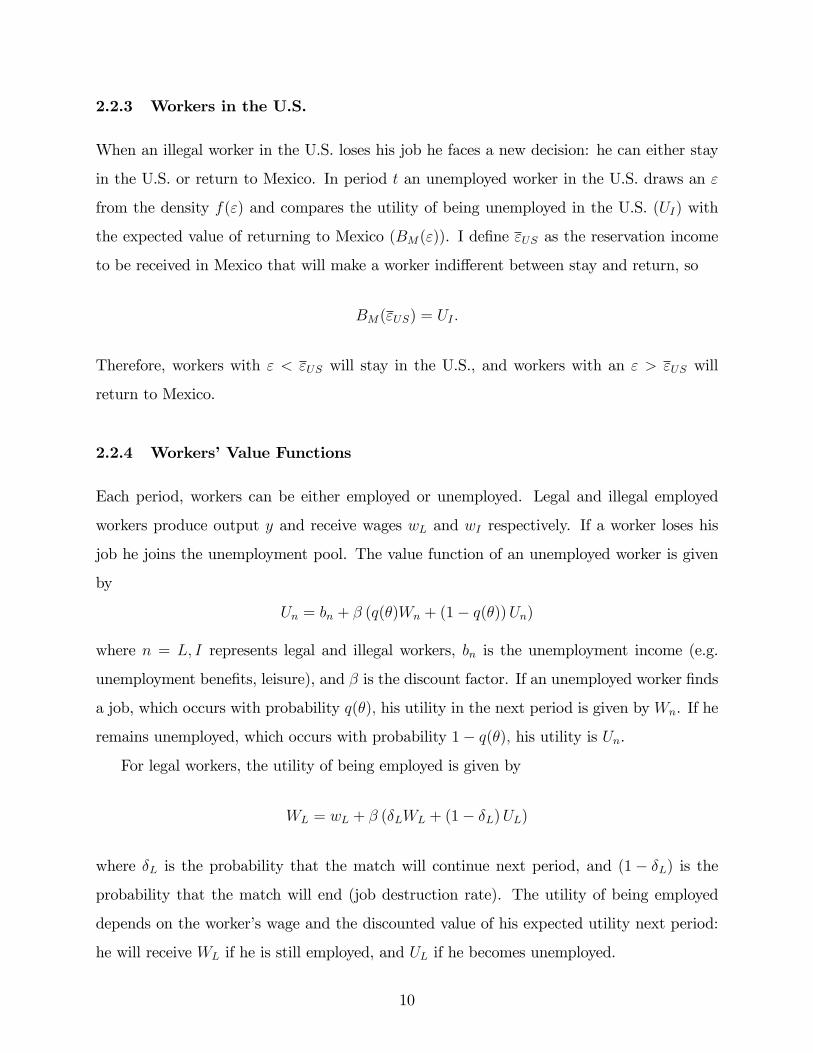
2.2.3 Workers in the U.S.
When an illegal worker in the U.S. loses his job he faces a new decision: he can either stay
in the U.S. or return to Mexico. In period t an unemployed worker in the U.S. draws an ε
from the density f(ε) and compares the utility of being unemployed in the U.S. (UI) with
the expected value of returning to Mexico (BM(ε)). I define εUS as the reservation income
to be received in Mexico that will make a worker indifferent between stay and return, so
BM(εUS) = UI .
Therefore, workers with ε < εUS will stay in the U.S., and workers with an ε > εUS will
return to Mexico.
2.2.4 Workers’Value Functions
Each period, workers can be either employed or unemployed. Legal and illegal employed
workers produce output y and receive wages wL and wI respectively. If a worker loses his
job he joins the unemployment pool. The value function of an unemployed worker is given
by
Un = bn + β (q(θ)Wn + (1− q(θ))Un)
where n = L, I represents legal and illegal workers, bn is the unemployment income (e.g.
unemployment benefits, leisure), and β is the discount factor. If an unemployed worker finds
a job, which occurs with probability q(θ), his utility in the next period is given by Wn. If he
remains unemployed, which occurs with probability 1− q(θ), his utility is Un.
For legal workers, the utility of being employed is given by
WL = wL + β (δLWL + (1− δL)UL)
where δL is the probability that the match will continue next period, and (1− δL) is the
probability that the match will end (job destruction rate). The utility of being employed
depends on the worker’s wage and the discounted value of his expected utility next period:
he will receive WL if he is still employed, and UL if he becomes unemployed.
10

For an illegal worker, the utility of being employed is given by
WI = wI + β(δIWI + (1− δI)UI
)where δI is the probability that the match will continue next period and (1− δI) is
their job destruction rate. His utility depends on his wage and the discounted value of his
expected utility next period. If the match continues he receives WI . Since an unemployed
illegal worker can stay in the U.S. or return to Mexico if he becomes unemployed, his utility
UI can be written as
UI = F (εUS)UI + (1− F (εUS))∞∫
εUS
BM(ε′)f(ε′|ε′ > εUS)dε
′.
If the worker stays in the U.S. his utility is UI and if he returns to Mexico his utility
is BM(ε). F (εUS) is the probability of having ε lower than εUS (the worker finds optimal
to stay in the U.S.), and (1 − F (εUS)) is the probability of having ε higher than εUS (the
worker finds optimal to return).
It is important to note that the job destruction rate is different between legal and ille-
gal workers and tends to be higher among undocumented workers due to law enforcement
(workers can be apprehended and deported) and to the presence of temporary workers (e.g.
target earners) in the U.S.
2.2.5 Firms’Value Functions
Each period firms post a certain number of vacancies (i.e. job openings) in search for workers
at a cost c per unit of time. The flow of new matches between firms and workers is determined
by a matching function. If a firm is matched with a legal or an illegal worker where n = L, I,
its value function is given by
Jn = y − wn + β (δnJn + (1− δn)V )
where y denotes the output produced, wn is the wage paid to each type of worker and V is
the value of a firm with an open vacancy. The value of a firm will be given by the output
produced net of wages plus the discounted value of the utility of the firm next period. If the
11
match continues, which occurs with probability δn, the value of the firm next period is Jn. If
the match ends, which occurs with probability (1− δn), the firm will have an open vacancy
and its utility will be V.
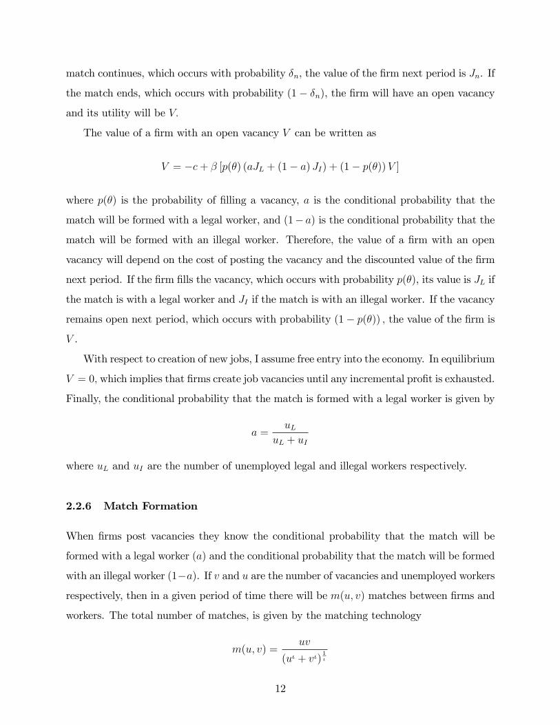
The value of a firm with an open vacancy V can be written as
V = −c+ β [p(θ) (aJL + (1− a) JI) + (1− p(θ))V ]
where p(θ) is the probability of filling a vacancy, a is the conditional probability that the
match will be formed with a legal worker, and (1− a) is the conditional probability that the
match will be formed with an illegal worker. Therefore, the value of a firm with an open
vacancy will depend on the cost of posting the vacancy and the discounted value of the firm
next period. If the firm fills the vacancy, which occurs with probability p(θ), its value is JL if
the match is with a legal worker and JI if the match is with an illegal worker. If the vacancy
remains open next period, which occurs with probability (1− p(θ)) , the value of the firm is
V .
With respect to creation of new jobs, I assume free entry into the economy. In equilibrium
V = 0, which implies that firms create job vacancies until any incremental profit is exhausted.
Finally, the conditional probability that the match is formed with a legal worker is given by
a =uL
uL + uI
where uL and uI are the number of unemployed legal and illegal workers respectively.
2.2.6 Match Formation
When firms post vacancies they know the conditional probability that the match will be
formed with a legal worker (a) and the conditional probability that the match will be formed
with an illegal worker (1−a). If v and u are the number of vacancies and unemployed workers
respectively, then in a given period of time there will be m(u, v) matches between firms and
workers. The total number of matches, is given by the matching technology
m(u, v) =uv
(uι + vι)1ι
12

where u = uL + uI . The matching technology is homogeneous of degree one, increasing and
concave in its two arguments, and exhibits constant returns to scale. This matching function
was chosen following the specification presented by Den Haan, Ramey and Watson (2000).
One of the advantages of using this function over the traditional Cobb-Douglas specification
is that this function guarantees matching probabilities between zero and one for all u and v.
Let θ = vube the vacancy-unemployment ratio (or labor market tightness). Then the
probability of filling a vacancy p(θ) is given by
p(θ) =m(u, v)
v,
and the probability of finding a job q(θ) is given by
q(θ) =m(u, v)
u= θp(θ) .
Note that p′(θ) < 0 and q′(θ) > 0. Therefore, the probability of filling a vacancy is higher
when the labor market is not tight and the probability of finding a job is higher when the
labor market is tight.
2.2.7 Wage Determination
Once a match has been formed, and the firm observes the worker’s type, wages are determined
by Nash bargaining. Firms and workers have to negotiate, and outside options are worse
than an agreement because both parties would need to search again. The Nash solution is
to set wL and wI to maximize the product surpluses
max wL(WL − UL)1−η(JL − V )η
and
max wI (WI − UI)1−η(JI − V )η,
where η is a bargaining parameter.
Solving for wL and wI I find that
wL = (1− η)y + η(1− β)UL
13

and
wI = (1− η)y + η(1− β)UI .
Notice that the wage depends on productivity as well as on workers’outside options.
The difference in the wages of legal and illegal workers
wL − wI = η(1− β)(UL − UI),
is proportional to the difference in the expected utility of unemployment of legal and illegal
workers. Therefore, we can identify two mechanisms that affect the wage gap between legal
and illegal workers:
1. If unemployed legal workers have higher utility flow than unemployed illegal workers the
wage gap will be higher. This is due to the fact that when bargaining with the firm,
legal workers have better outside options than illegal workers, so they get higher wages.
2. If the probability of being terminated is higher for illegal workers, then undocumented
workers have a lower utility from being unemployed because their employment relation-
ships are short-lived.
2.2.8 Equilibrium Steady State
In steady state, the flows into and out of unemployment are equal. The steady state condition
for unemployment of legal workers is given by
uL = uL (1− q(θ)) + (1− δL)(µL − uL)
where µL is the number of legal workers and uL is the number of unemployed legal workers.
Each period the number of unemployed workers equals the number of workers who were
unemployed last period and did not find a job, and the workers who were employed last
period (µL − uL) and lost their job.
The steady state condition for unemployment of illegal workers is given by
uI = uI (1− q(θ)) + (1− δI)eIF (εUS) + (µI − uI − eI)F (εM)
14

where µI is the total number of Mexican workers (in Mexico or the U.S.), and uI and eI are
the number of unemployed and employed Mexican illegal workers in the U.S.
Each period the number of unemployed illegal workers in the U.S. equals the number
of workers who were unemployed last period and did not find a job, the workers who were
employed last period, lost their job, and decided to stay in the U.S., and the workers from
Mexico who decided to migrate this period.
In steady state the flow of workers entering the U.S. must equal the flow of workers
leaving the country. Therefore, the steady state condition is given by
(1− δI)(1− F (εUS))eI = (µI − uI − eI)F (εM)
where the number of workers who lost their job and return to Mexico is equal to the number
of workers who decided to migrate to the U.S.
2.3 DISCUSSION OF THE EFFECTS OF POLICIES
2.3.1 Effects of an Amnesty
In this section I discuss quantitatively the effect of an amnesty granting legal status to a
proportion of the illegal population in the economy. Since the model cannot be solved ana-
lytically, I provide intuition on the implications of this policy on the labor market outcomes
of natives and immigrants.
An amnesty decreases the number of illegal workers and increases the number of legal
workers in the economy. According to the model, a decrease in the number of illegal workers
would decrease firms’incentives to post vacancies since firms’probability of finding a worker
with a low outside option decreases. The decrease in the number of vacancies decreases
labor market tightness (θ) , the probability of finding a job (q(θ)), and therefore, increases
the unemployment rate of both legal and illegal workers (uL and uI).
With respect to wages the model predicts that the decrease in the probability of finding
a job (q(θ)) will worsen workers’outside options decreasing the wages received by both types
of workers (wL and wI).
15

In this model the presence of illegal workers in the economy has a positive effect on the
wages of natives in the long run. This is consistent, although due to a different mechanism,
to the result of Ottaviano and Peri (2010). They find that the 1990-2006 immigration wave
to the U.S. will have a small positive effect on the average wages of natives due to imperfect
substitution of immigrants for natives.
2.3.2 Effects of an Increase in Border Enforcement
I capture the effect of an increase in border enforcement by changing migration costs. The
model predicts that higher migration costs (measured in months of earnings in Mexico)
would decrease εM which implies that less individuals would find optimal to migrate. With
respect to the workers in the U.S., the model predicts that εUS increases and more workers
find optimal to stay in the U.S. Therefore, the overall effect of an increase in migration costs
in the number of illegal workers in the U.S. is ambiguous.
If the overall effect is an increase in the illegal population, the model predicts that firms
will have incentives to increase the number of vacancies since firms’probability of finding
workers with a low outside option increases. The increase in the number of vacancies increases
labor market tightness (θ) , the probability of finding a job (q(θ)), and therefore, decreases
the unemployment rate of both legal and illegal workers (uL and uI).
With respect to wages of legal workers (wL) the model predicts that the increase in
the probability of finding a job (q(θ)) will improve workers’outside options increasing their
wages.
Finally, for illegal workers the model predicts that the effect of tighter border enforcement
has an ambiguous effect on their wages. On the one hand, the increase in the probability of
finding a job (q(θ)) improves workers’outside options increasing their wages. However, the
increase in migration costs also worsens workers’outside options (workers are less likely to
undertake multiple trips to the U.S.) decreasing their wages.
16

Table 1: Parameters and Calibrated Targets
Parameter Value Source
Output y = 1 Normalization
Discount Factor K = 0.996 Pissarides (09)
Bargaining parameter R = 0.5 Pissarides (09)
Unemp Income/Leisure Legal b L = 0.71 Hal & Milgrom (08)
Destruction rate Legal 1 ? NL = 0.034 Shimer (04)
Destruction rate Illegal 1 ? NI = 0.063 EMIF 9305
Migration costs K = 4 EMIF 9305
Legal Population US WL = 0.9 CPS 0010
Mexican Population WI = 0.1 ENNVIH 2002, DHS(05&06)
Parameter Value Calibration Target
Vacancy cost c = 0.377 Wage gap w Lw I
? 1 = 0.09
Distribution parameter P2 = 1.51 Wage gap w Mexw US
? 1 = ?0.84
Leisure Illegal b I = 0.235 Unemployment rate u = 0.10
Parameter Matching Function T = 0.691 Market tightness S = 0.72
2.4 QUANTITATIVE ANALYSIS
Next, I use the model to quantitatively assess the effect of an amnesty and tighter border en-
forcement. I fix some parameters apriori using values typically used in Mortensen-Pissarides
style models, a second group of parameters are set using different data sources on illegal
immigration, and finally a third group of parameters are calibrated to match some targets
in the data. The parameters and calibration targets are summarized in Table 1.
Since legal and illegal workers are assumed to be equally productive, I set the output
produced by both types of workers to y = 1. The time unit is a month, therefore, the
discount factor β = 0.996 reflects an annual discount rate of 4.8 percent (Pissarides (2009)).
I give the worker and firm equal bargaining power by setting η = 0.5 (Pissarides (2009)). The
income equivalent that unemployed legal workers give up to take a job is set at bL = 0.71.
It includes both unemployment insurance and the value of time (Hall and Milgrom (2008)).
Finally, the job separation rate for legal workers (1− δL) is set to 0.034 which implies that
among legal workers jobs last for about 2.5 years on average (Shimer (2005)).
17
In order to estimate the job separation rate for illegal workers I use information from the
Survey of Migration to the Northern Border (EMIF). The EMIF is a cross-sectional survey
conducted ten times between 1993 and 2005 that samples the flows of immigrants between
Mexico and the U.S. in the northern border region of Mexico.9 Using a subsample of 5,752
Mexican male illegal workers interviewed between 1993 and 2005 who were employed at the
time of the survey in the U.S. and report information on the duration of their longest job
held in the U.S., I estimate an average job duration of 15.8 months and set the job separation
rate for legal workers (1− δI) to 0.063.10
Migration costs in months of earnings in Mexico (K) are estimated using transportation
cost, smuggler fees and other expenses incurred during the trip. Data on smuggler fees,
other expenses, average distance from the city of origin to the city of destination, and
average monthly earnings in Mexico prior migration are obtained from the EMIF. Estimates
on the transportation cost per mile from Mexico to the U.S. are estimated using information
from different transportation companies in Mexico and the U.S. The estimates show that on
average, migration costs for workers who entered between 1998 and 2005 were 4 months of
their income prior migration.11
The proportion of legal and illegal workers in the economy µL and µI are set at 0.9 and
0.1 respectively. While µL represents the number of legal workers in the U.S., µI represents
the number of Mexican workers in the U.S. and in Mexico (potential migrants). Using in-
formation from the 2000 Mexican and U.S. Censuses I find estimates of their labor force. In
order to find an estimate of the number of workers in Mexico who can potentially migrate, I
use information from the Mexican Family Life Survey (MxFLS). This representative Mexi-
can survey devotes a section to analyze migration behavior and specifically asks individuals
if they would like to migrate. According to the survey, 15 percent of the individuals sur-
veyed reported intention to migrate.12 Finally, estimates from the Department of Homeland9The survey is conducted in eight Mexican border cities. Within each city, individuals are sampled at
different locations including bus stations, airports, train stations, international bridges, ports of entry andMexican customs inspection stations. The EMIF identifies illegal, temporary workers and return migrants.10Using information from the EMIF I also estimate the job separation rate for legal immigrants (1−δL) =
0.0312. This result is in line with the one obtained by Shimer (2005) for U.S. workers of (1− δL) = 0.034.11Migrants paid on average $960 (in 2001 US dollars) in smuggler fees, $170 (in 2001 U.S. dollars) in
transportation and other expenses, while their average monthly income prior migration was $270 (in 2001US dollars).12There are other two surveys that inquire about the individuals desire to migrate. According to the
18
Security show that in 2000 the number of illegal workers in the U.S. was 4.7 million.
The last group of parameters c, ε2, bI and ι are chosen calibrating them to match the
wage gap between legal and illegal workers, the wage gap between Mexico and the U.S., the
U.S. unemployment rate, and labor market tightness. Using information from the EMIF, I
estimate a wage gap between legal and illegal Mexican migrants of 9 percent for the period
between 1993 and 2005. The second target to match is the wage gap between workers in
Mexico and in the U.S. Using census data for Mexico and the U.S. in 2000 I find that
average wages in Mexico are 84 percent lower than those obtained by recent immigrants
in the U.S. With respect to the unemployment rate, several authors have argued that the
targeted steady state rate of unemployment should include more than the rate of workers
counted as unemployed as the model does not account for non-participation. For example,
Krause and Lubik (2007) chose an unemployment rate of 12 percent, Den Haan, Ramey
and Watson (2000) 11 percent, Petrosky-Nadeau (2009) 10 percent, and Gertler and Trigari
(2009) 7 percent. Using a midpoint between the later authors I set the unemployment rate
of 10 percent. Finally, I set (θ) = 0.72, the sample mean for the market tightness between
1960 and 2002 estimated by Pissarides (2009).13
The calibrated parameters are the following. The vacancy posting cost per period is
c = 0.377 (close to the 0.356 found by Pissarides (2009)), the upper bound of the distribution
of epsilon is set to ε2 = 1.51,14 the unemployment income for unemployed illegal workers
(leisure) obtained in the calibration is bI = 0.235, and the parameter matching function ι
= 0.691.
2007 Gallup World Poll "Mexicans and Migration", 9.5% of the individuals surveyed would like to movepermanently to the US if they had the opportunity. A second survey is the Latinobarómetro public opinionsurvey. This survey reports that 10.5% of the individuals surveyed in Mexico in 2002 responded that theyand their families have seriously considered migrating to the U.S. These surveys report estimates lower thanthose from the MxFLS. While the Gallup Survey refers exclusively to permanent migrations, Latinobarómetrorefers to migration decision of complete families.13This value is estimated by using Job Openings and Labor Turnover Survey (JOLTS) data since December
2000 and the Help-Wanted Index (HWI) adjusted to the JOLTS units of measurement before then (Pissarides(2009)).14Epsilon (ε) follows a uniform distribution between ε1 and ε2.
19

Table 2: Model’s Predictions - Amnesty Decreasing the Illegal Population by 50 percent
μI=0.1 μI=0.05 DifferenceVacancy/unemployment ratio 0.720 0.660 0.060Probability of filling vacancy 0.428 0.445 0.017Probability of finding a job 0.308 0.294 0.015
Unemployment rate legal 9.93% 10.38% 0.45%
Unemployment rate illegal 17.0% 17.7% 0.70%
Wage legal 0.971 0.970 0.12%
Wage illegal 0.891 0.889 0.27%
Wage initially illegal 0.891 0.929 4.32%
Wage gap 9.01% 9.17% 0.16%Average wage 0.965 0.967 0.24%Welfare employed legal 236.4 235.9 0.23%Welfare employed illegal 197.2 196.0 0.59%Welfare unemployed legal 235.7 235.1 0.24%Welfare unemployed illegal 195.4 194.1 0.63%
2.4.1 Results: Effect of an Amnesty
Table 2 shows the effect of an amnesty granting legal status to 50 percent of the illegal
population. The results show that this policy would decrease market tightness, increase
the probability of filling a vacancy p(θ) from 42.8 percent to 44.5 percent, and decrease the
probability of finding a job q(θ) from 30.8 percent to 29.4 percent. The decrease in the
probability of finding a job increases the unemployment rate of legal workers by 0.45 percent
and the unemployment rate of illegal workers by 0.70 percent. The results also show that
the presence of illegal workers have a positive effect on the wages of natives. The amnesty
would decrease the wages of natives by 0.12 percent and decrease the wages of illegal workers
by 0.27 percent. Figure 1 shows the effect of an amnesty granting legal status to different
proportions of the illegal population in the U.S.15
15The horizontal axis of Figure 1 indicates the proportion of the illegal workers remaining after the amnesty.The graph on top shows the unemployment rates of legal (natives) and illegal workers. The graph in thebottom shows the wages of legal (natives) and illegal workers. In the baseline scenario the population illegalworkers is set at 10 percent.
20
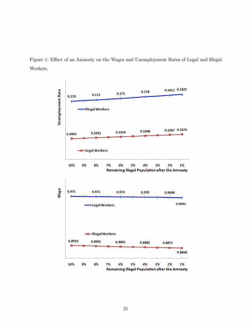
Figure 1: Effect of an Amnesty on the Wages and Unemployment Rates of Legal and Illegal
Workers.
21

Table 3: Model’s Predictions - Tighter Border Enforcement Increasing Migration Costs
4 8Vacancy/unemployment ratio 0.720 0.734 0.014Probability of filling vacancy 0.428 0.425 0.016Probability of finding a job 0.308 0.312 0.015Unemployment rate legal 9.9% 9.8% 0.09%Unemployment rate illegal 17.0% 16.8% 0.15%Wage legal 0.971 0.972 0.03%Wage illegal 0.891 0.887 0.45%Wage gap 9.0% 9.5% 0.5%Average wage 0.965 0.964 0.04%Optimal to migrate US (εM) 0.281 0.229 0.052Optimal to stay in US (εUS) 0.844 1.147 0.302Proportion of illegal workers US 8.9% 9.2% 0.3%Welfare employed legal 236.4 236.5 0.05%Welfare employed illegal 197.2 195.2 0.98%Welfare unemployed legal 235.7 235.8 0.05%Welfare unemployed illegal 195.4 193.5 0.97%
Migration Costs (Monthsof Earnings in Mexico) Difference
2.4.2 Results: Effect of Tighter Border Enforcement
Table 3 shows the effect of an increase in border enforcement that doubles migration costs.
Migration costs are measured in months of earnings in Mexico prior migration. The results
show that this policy would decrease market tightness, decrease the probability of filling a
vacancy p(θ) from 42.8 percent to 42.5 percent, and increase the probability of finding a
job q(θ) from 30.8 percent to 31.2 percent. The increase in the probability of finding a job
decreases the unemployment rate of legal workers by 0.09 percent and the unemployment
rate of illegal workers by 0.15 percent.
The results show that higher migration costs decrease εM and increase εUS, which implies
that fewer individuals in Mexico find it optimal to migrate and more workers in the U.S. find
it optimal to stay in the U.S. The overall effect of the increase in border enforcement is an
increase in the number of illegal workers in the U.S. (eI+uI) from 8.9 percent to 9.2 percent.
These results highlight the importance of accounting for return migration when estimating
22

Figure 2: Effect of Tighter Border Enforcement on Wages and Unemployment Rates for
Legal and Illegal Workers.
23

the effects of different immigration policies. While tighter border enforcement deters workers
from crossing, it also decreases return migration increasing the illegal population in the U.S.
The results also show that the increase in the illegal population in the U.S. increases the
wages of natives by 0.03 percent. The increase in the probability of finding a job improves
workers’outside options, and therefore, increases their wages.
Finally, with respect to the wages of illegal workers, the increase in migration costs
generates two opposing effects on workers’outside options, and therefore, on their wages:
on the one hand, the increase in the probability of finding a job improves workers’outside
options, on the other hand, higher migration costs worsen workers’outside options since
workers are less likely to undertake multiple trips to the U.S. The results show that the latter
effect dominates; doubling migration costs due to tighter border enforcement decreases the
wages of illegal workers by 0.45 percent.16
2.5 MODEL WITH ILLEGAL WORKERS PAYING PAYROLL TAXES
While some illegal workers, such as day laborers and domestic workers are paid in cash off
the books, estimates suggest that between 50 and 75 percent of the undocumented workers in
the U.S. pay payroll taxes.17 Illegal workers frequently obtain formal jobs using false social
security numbers or social security numbers that belong to someone else. They have payroll
taxes withheld as any other legal worker in the U.S., however, in order to avoid detection,
they do not file for tax refunds or unemployment benefits.
In the following section I modify the model to study the effect of an amnesty in an
economy where firms can hire illegal workers "off the books", paying them under the table
and avoiding the payment of payroll taxes; or "on the books", using false social security
16Figure 2 shows the effect of increases in border enforcement measured by increases in migration costs.Migration costs are measured in months of earnings in Mexico (horizontal axis). The graph at the top showsthe unemployment rates of legal (natives) and illegal workers. The graph at the bottom shows the wages oflegal (natives) and illegal workers. In the baseline scenario migration cost are set at 4 months of earnings.17According to Stephen Goss, chief actuary with the Social Security Administration, as many as 75 percent
of the undocumented workers pay payroll taxes (Porter (2005)). A recent review by the Congressional BudgetOffi ce (2007) shows that income tax compliance rates are typically estimated to fall between 50 and 75 percentamong unauthorized immigrants.
24
numbers pretending they are legal aliens.
2.5.1 Model
For simplicity, I will assume that there is no movement of workers between Mexico and
the U.S. Each period firms post a certain number of vacancies and a matching function
determines the flow of new matches between firms and workers. When firms post vacancies,
they only know the conditional probability that the match will be formed with a legal or an
illegal worker. Once the match is formed, firms realize the worker’s type. If the match is
done with an illegal worker, the firm decides if the worker is hired on or off the books.
In this setting a fixed payroll tax (T ) is levied on firms for all legal workers and for the
illegal workers hired on the books. The tax revenue is used to pay for the unemployment
benefits of legal workers (bU). Now, the income of unemployment of legal workers will include
two components: income received from unemployment insurance (bU) and the value of leisure
(bO). For illegal workers, the income of unemployment will be the value of leisure (bI). The
value functions of unemployed legal and illegal workers are given by
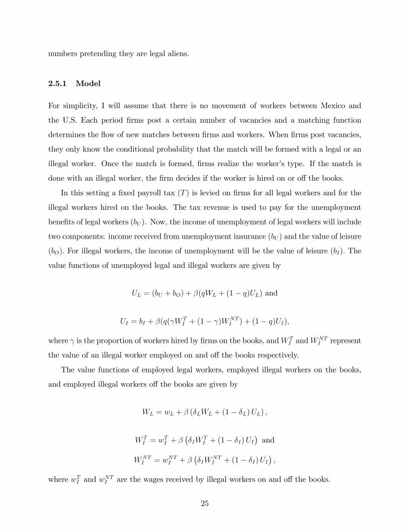
UL = (bU + bO) + β(qWL + (1− q)UL) and
UI = bI + β(q(γW TI + (1− γ)WNT
I ) + (1− q)UI),
where γ is the proportion of workers hired by firms on the books, andW TI andW
NTI represent
the value of an illegal worker employed on and off the books respectively.
The value functions of employed legal workers, employed illegal workers on the books,
and employed illegal workers off the books are given by
WL = wL + β (δLWL + (1− δL)UL) ,
W TI = wTI + β
(δIW
TI + (1− δI)UI
)and
WNTI = wNTI + β
(δIW
NTI + (1− δI)UI
),
where wTI and wNTI are the wages received by illegal workers on and off the books.
25

The firm’s value functions are given by
JL = y − wL − T + β (δLJL + (1− δL)V ) ,
JTI = y − wTI − T + β(δIJTI + (1− δI)V ) and
JNTI = y − wNTI + β(δIJ
NTI + (1− δI)V
),
where JTI and JNTI represent the value of a firm matched with an illegal worker on and off
the books, and T is the amount of the payroll tax.
The value of a firm with an open vacancy can be written as
V = −c+ βp(aJL + (1− a)
{γJTI + (1− γ)JNTI
})+ β (1− p)V
where p(θ) is the probability of filling a vacancy, (1− a) is the conditional probability that
the match will be formed with an illegal worker, and γ is the conditional probability that
the match with the illegal worker will be on the books. With respect to creation of new jobs
I assume free entry into the economy, which implies that firms create job vacancies until any
incremental profit is exhausted (V = 0).
Wages are determined by Nash bargaining, the solution is to set wL, wTI and wNTI to
maximize the product surpluses
maxwL(WL − UL)1−η(JL − V )η,
maxwNTI
(WNTI − UI)1−η(JNTI − V )η and
maxwTI
(W TI − UI)1−η(JTI − V )η.
In this model, the payroll tax is used to pay for the unemployment benefits of legal workers. In
steady state, tax revenue must equal tax expenditures. Therefore, the steady state condition
is given by
uLbL = T (µL − uL) + Tγ(µI − uI)
where the expenditure in unemployment benefits for legal workers is equal to the tax revenue
generated by the payroll tax levied on legal workers and on illegal workers on the books.
26
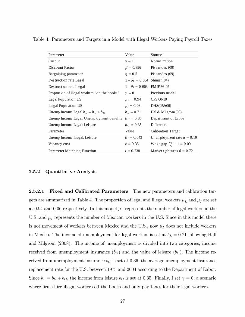
Table 4: Parameters and Targets in a Model with Illegal Workers Paying Payroll Taxes
Parameter Value Source
Output y = 1 Normalization
Discount Factor K = 0.996 Pissarides (09)
Bargaining parameter R = 0.5 Pissarides (09)
Destruction rate Legal 1 ? NL = 0.034 Shimer (04)
Destruction rate Illegal 1 ? NI = 0.063 EMIF 9305
Proportion of illegal workers "on the books" L = 0 Previous model
Legal Population US WL = 0.94 CPS 0010
Illegal Population US WI = 0.06 DHS(05&06)
Unemp Income Legal b L = b U + b O b L = 0.71 Hal & Milgrom (08)
Unemp Income Legal: Unemployment benefits b U = 0.36 Department of Labor
Unemp Income Legal: Leisure b O = 0.35 Difference
Parameter Value Calibration Target
Unemp Income Illegal: Leisure b I = 0.043 Unemployment rate u = 0.10
Vacancy cost c = 0.35 Wage gap w Lw I
? 1 = 0.09
Parameter Matching Function T = 0.738 Market tightness S = 0.72
2.5.2 Quantitative Analysis
2.5.2.1 Fixed and Calibrated Parameters The new parameters and calibration tar-
gets are summarized in Table 4. The proportion of legal and illegal workers µL and µI are set
at 0.94 and 0.06 respectively. In this model µL represents the number of legal workers in the
U.S. and µI represents the number of Mexican workers in the U.S. Since in this model there
is not movement of workers between Mexico and the U.S., now µI does not include workers
in Mexico. The income of unemployment for legal workers is set at bL = 0.71 following Hall
and Milgrom (2008). The income of unemployment is divided into two categories, income
received from unemployment insurance (bU) and the value of leisure (bO). The income re-
ceived from unemployment insurance bU is set at 0.36, the average unemployment insurance
replacement rate for the U.S. between 1975 and 2004 according to the Department of Labor.
Since bL = bU + bO, the income from leisure bO is set at 0.35. Finally, I set γ = 0; a scenario
where firms hire illegal workers off the books and only pay taxes for their legal workers.
27

The parameter of the matching function is set at ι = 0.738, the vacancy posting cost is
set at c = 0.35, and the income of unemployment for illegal workers is set at bI = 0.043.
These parameters are chosen calibrating them to match the wage gap between legal and
illegal workers (wLwI− 1 = 0.09), the U.S. unemployment rate (u = 0.10) and labor market
tightness (θ = 0.72). The targets used for the calibration are the same used in the previous
specification of the model. While the first two calibrated parameters are similar to the ones
obtained in section 2.4, the income of unemployment for illegal workers is significantly lower
because this new setting does not account for the possibility of return migration and illegal
workers have less alternative options.
2.5.2.2 Results: Changes in the Proportion of Illegal Workers Paying Payroll
Taxes Table 5 shows the effect of changes in the proportion of illegal workers paying payroll
taxes or on the books (γ) .18 The results show that illegal workers in jobs off the books earn
higher wages than illegal workers on the books since a proportion of the payroll tax levied
on the last group is transferred to workers.
The results show that an increase in the proportion of illegal workers on the books
decreases market tightness (θ) , decreases the probability of finding a job q(θ), and increases
unemployment rates.
Changes in the proportion of illegal workers on the books will affect wages in two ways:
First, the decrease in market tightness and increase of the unemployment rates worsen work-
ers’ outside options decreasing their wages (outside options effect). Second, the increase
in the number of illegal workers on the books will increase tax revenue because now more
workers pay the payroll tax (tax effect). Since illegal workers are not eligible for unemploy-
ment benefits, the amount of the tax necessary to pay for the unemployment benefits of legal
workers decreases. Since part of the tax is paid by firms and part is paid by workers in form
of lower wages, the increase in γ will increase the wages of the workers subject to payroll
taxes (legal workers and illegal workers on the books).
While we can conclude that the wages of illegal workers off the books will decrease due
18The wage gap between legal and illegal workers is calculating according to (wL/((γwTI + (1− γ)wNTI )−1. The welfare for employed legal workers (WI) is given by (γWT
I + (1− γ)WNTI ).
28

Table 5: Effect of Changes in the Proportion of Illegal Workers Paying Payroll Taxes
0 0.25 0.5 0.75 1Vacancy/unemployment ratio 0.720 0.719 0.718 0.7175 0.7167Probability of filling vacancy 0.4559 0.4561 0.4564 0.4566 0.4568Probability of finding a job 0.3282 0.3280 0.3278 0.3276 0.3274Unemployment rate legal 9.386% 9.392% 9.397% 9.403% 9.408%Unemployment rate illegal 16.10% 16.11% 16.12% 16.13% 16.14%Wage legal 0.9389 0.9394 0.9398 0.9403 0.9407Wage illegal "off" the books 0.861 0.858 0.855 0.852 0.848Wage illegal paying tax 0.843 0.840 0.837 0.834 0.831Wage gap 9.0% 10.1% 11.1% 12.2% 13.2%Average wage 0.93429 0.93424 0.93419 0.93415 0.93411Tax 0.0373 0.0368 0.0363 0.0358 0.0353Tax revenue 0.03176 0.03178 0.03180 0.03182 0.03184Welfare employed legal 229.4 229.5 229.6 229.7 229.8Welfare employed illegal 182.7 181.0 179.4 177.8 176.2Welfare unemployed legal 228.8 228.9 229.0 229.1 229.2Welfare unemployed illegal 180.6 179.0 177.3 175.8 174.2
Proportion of Illegal Workers Paying Payroll Taxes
to the lower outside options effect, the impact on the wages of legal workers and illegal
workers on the books will depend on the magnitude of the two effects (lower outside options
effect and tax effect). Table 5 shows that for legal workers the tax effect dominates, and an
increase of γ increases their wages (wL). On the other hand, for illegal workers on the books
the outside option effect dominates and an increase of γ decreases their wages (wTI ).
2.5.2.3 Results: Effect of an Amnesty Table 6 shows the effect of an amnesty de-
creasing the illegal population from 6 percent to 1 percent for different values of γ (propor-
tion of illegal workers on the books). Column A shows the baseline scenario when all illegal
workers are paid under the table (γ = 0) and column B shows the effects of the amnesty on
different variables with respect to the baseline scenario. Columns C through F show baseline
scenarios and effects of the amnesty for γ = 0.5 and γ = 1.19
19Table 26 in the Appendix shows the effects of an amnesty, first, if we leave the amount of the payrolltax fixed, and second, if we allow the tax to adjust to make the revenue from payroll taxes equal to the
29

Table 6: Effect of an Amnesty in a Model with Illegal Workers Paying Payroll Taxes
A B C D E FBaseline Difference Baseline Difference Baseline Difference
Proportion workers paying tax 0 0 0.5 0.5 1 1Vacancy/unemployment ratio 0.720 0.137 0.718 0.135 0.7167 0.1338Probability of filling vacancy 0.4559 0.0422 0.4564 0.0418 0.4568 0.0415Probability of finding a job 0.3282 0.0376 0.3278 0.0373 0.3274 0.0370Unemployment rate legal 9.39% 1.09% 9.40% 1.08% 9.41% 1.07%Unemployment rate illegal 16.10% 1.71% 16.12% 1.70% 16.14% 1.69%Wage legal 0.9389 0.72% 0.9398 0.80% 0.9407 0.87%Wage illegal "off" the books 0.8613 1.43% 0.8547 1.51% 0.8485 1.64%Wage illegal paying tax 0.8426 1.75% 0.8366 1.89% 0.8308 2.06%Wage gap 9.02% 0.78% 11.14% 1.02% 13.22% 1.37%Average wage 0.9343 0.314% 0.9342 0.307% 0.9341 0.300%Tax 0.037 12.95% 0.036 15.64% 0.035 18.30%Tax revenue/expenditure 0.03176 17.53% 0.03180 17.42% 0.03184 17.32%Welfare employed legal 229.4 0.93% 229.6 1.00% 229.8 1.06%Welfare employed illegal 182.7 3.26% 179.4 3.51% 176.2 3.85%Welfare unemployed legal 228.8 0.95% 229.0 1.0% 229.2 1.09%Welfare unemployed illegal 180.6 3.4% 177.3 3.6% 174.2 4.0%
The results show that an amnesty decreases the probability of finding an illegal worker
with a low outside option and therefore, decreases θ. The decrease in θ generates an increase
in unemployment. According to the model, the decrease in θ will be smaller for larger values
of γ. If γ is low, which implies, a large number of illegal workers are employed off the books,
an amnesty reducing the illegal population will generate a large decrease in θ. On the other
hand, if γ is high, and therefore, a large proportion of the illegal workers work on the books
(and firms are already paying taxes for those workers), the amnesty will generate a smaller
decrease in the number of vacancies and θ.
The decrease in θ decreases the probability of finding a job (q) and increases the unem-
ployment rate of legal and illegal workers. Since the decrease of θ is smaller for large values
of γ, the increase in unemployment rates will also be smaller for higher values of γ.
expenditure of unemployment benefits for all legal workers. The results show that the tax adjustment furtherdecreases the wages of all types of workers as result of the amnesty.
30

Effect of an Amnesty on the Wages of Legal Workers
The wages of legal workers are affected in two ways. First, the increase in the unemploy-
ment rate worsens workers’outside options decreasing their wages (outside options effect).
Additionally, the fact that now there is a larger number of unemployed legal workers, the
amount of the tax necessary to pay for unemployment benefits will go up, decreasing even
more the wages of legal workers (tax effect).
The magnitude of the decrease in the wages of legal workers for different values of γ
depends on the magnitude of the outside options effect and the tax effect. On the one hand,
the decrease of θ and the increase in unemployment rates are smaller for large values of γ.
Therefore, the decrease in wages due to worse outside options should be lower for high values
of γ. On the other hand, an amnesty increasing the legal population increases the number
of workers paying taxes but also the number of workers claiming unemployment benefits.
If a large proportion of illegal workers were paying the tax before the amnesty (high γ),
the amnesty will only increase unemployment claims, and therefore, the amount of the tax.
Since part of the tax is paid by the firm and part of the tax is paid by workers, a higher tax
implies lower wages for legal workers. The results show that the second effect dominates,
and the decrease in the wages of legal workers is larger for higher values of γ.
Effect of an Amnesty on the Wages of Illegal Workers Paying Payroll Taxes
The decrease in their wages is larger than that observed among legal workers but due to
the same mechanisms. First, higher unemployment rates worsen outside options decreasing
their wages, and second, due to higher taxes necessary to pay for unemployment benefits of
the newly legalized immigrants. The magnitude of the decrease in their wages for different
values of γ depends on the magnitude of the outside options effect and the tax effect (the
outside options effect is larger for low γ but the tax effect is smaller for low γ). The results
show that the tax effect dominates, and the decrease in the wages of illegal workers on the
books is larger for higher values of γ.
Effect of an Amnesty on Wages of Illegal Workers off the Books
The decrease in their wages is larger than that observed among legal workers, but lower
31

than those observed among illegal workers on the books. The reason is that they are only
affected by the first mechanism (decrease in outside options). Since they are working off the
books, the increase in taxes necessary to pay for unemployment benefits does not affect their
wages. The results show that an amnesty would decrease the wages of illegal workers off the
books, and the effect is going to be larger for low values of γ.
Summarizing, it is important to account for the fact that a proportion of illegal workers
are working on the books and therefore pay payroll taxes in order to measure the effect of
an amnesty on the wages of workers. The results show that the larger the proportion of
illegal workers paying taxes, the larger will be the amount of the tax necessary to pay for
the increase in unemployment claims (the amnesty will not change the number of workers
paying taxes but will increase the number of workers claiming for unemployment benefits),
and therefore, the larger will be the decrease in the wages of legal and illegal workers in the
economy.
2.6 CONCLUSIONS
I analyze the effects of two immigration policies, an amnesty and an increase in border
enforcement, on the labor market outcomes of U.S. natives and Mexican immigrants. Even
though changes to the immigration system have potentially large implications, little research
has been devoted to analyze the effects of different policies on the U.S. labor market. In
this paper I use a Mortensen-Pissarides style labor market model to estimate the effects of
those policies on the wages and unemployment of legal and illegal workers. One distinctive
characteristic of my model is that it accounts for return migration, an important feature
when studying illegal immigration due to the high mobility between Mexico and the U.S.
observed among undocumented workers.
This paper highlights a new channel through which natives and illegal workers interact in
the economy. In this model, natives benefit from the presence of illegal workers in the labor
market. The presence of illegal workers increases firm’s incentives to open vacancies (since
32

their probability of finding a worker with a low outside option increases), which increases
the wages of natives and decreases their unemployment rate. Hence, an amnesty granting
legal status to a proportion of the illegal population would decrease the wages of natives and
increase their unemployment rate.
Moreover, this paper points out the fact that immigration policies might have unintended
effects. The model shows that an increase in border enforcement has an ambiguous effect
on the number of illegal workers in the economy. While tighter border enforcement deters
illegal migration of prospective workers, it also changes incentives for those already in the
U.S. by decreasing return migration. In the event that tighter border increases the number
of illegal workers, the model predicts that it will increase the wages of natives and have
an ambiguous effect on the wages of illegal workers. Quantitative results show that tighter
border enforcement increases the number of illegal workers, increases the wages of natives
and decreases the wages of illegal workers.
These results are consistent with the findings of existing studies. The fact that natives
benefit from the presence of illegal workers in the labor market is in line, although due
to a different mechanism, to the result of Ottaviano and Peri (2010). They find that the
1990-2006 immigration wave to the U.S. will have a small positive effect on the average
wages of natives in the long run. Moreover, relative to the ambiguous effect of tighter border
enforcement on the flows of illegal immigrants, my results are in line with the findings of
Angelucci (2005). She studies the impact of enforcement on 1972-1993 migration net flows
finding that increases in border controls deter migrants from crossing the border illegally,
but lengthen their duration in the U.S.
Additionally, in this paper I emphasize the importance of accounting for the fact that
a proportion of illegal workers have formal jobs and pay payroll taxes. The results show
that the smaller the proportion of illegal workers paid off the books, the larger will be the
decrease in wages generated by a decrease in the number of illegal workers in the economy.
There are three extensions to this paper that are of potential interest. First, relax the
assumption of having constant returns to scale in the aggregate economy. The results of this
model represent the long run equilibrium where we have a perfectly elastic capital supply
and do not consider the negative effect of having more workers in the economy in the short
33

run.
Second, allow some Mexican immigrants to enter the U.S. legally (e.g. workers with
temporary work permits or workers with tourist visas), and then overstay. Even though
these workers represent a small fraction of the illegal immigrant population in the U.S., their
expected utility of working illegally in the U.S. is higher than that of workers who enter
illegally and could impact workers’behavior.
Finally, it would also be interesting to investigate the effect of alternative immigration
policies, for example, policies intended to change firms’ incentives to hire illegal workers.
Such policies include the implementation of audits and workplace raids to firms suspected of
hiring illegal workers, or increases in penalties to firms hiring illegal workers. Even though the
Immigration Reform and Control Act of 1986 (IRCA) legally mandates that U.S. employers
verify the employment eligibility status of newly-hired employees, the implementation and
enforcement of such policies have not been successful in the past.
34

3.0 EFFECT OF LEGAL STATUS ON THE WAGES OF MEXICAN
IMMIGRANTS IN THE UNITED STATES
3.1 INTRODUCTION
Immigration from Mexico to the United States (U.S.) is a topic of great interest for policy-
makers and academics. Mexico is the most important source country for U.S. immigration,
accounting for 34.0 percent of total immigrant arrivals since 1990.1 In 2009, the 11.5 mil-
lion Mexican immigrants living in the U.S. represented 29.9 percent of the U.S. foreign-born
population and 10.6 percent of the total population of Mexico.2 One important feature of
Mexican immigration is that a high percentage of new arrivals enter the U.S. illegally.3 Esti-
mates from the Department of Homeland Security (DHS) suggest that in January 2010 the
number of illegal Mexican workers in the U.S. was 6.6 million, which represents 61.5 percent
of the total unauthorized population in the U.S.4
Even though the evidence has shown that legal workers earn on average higher wages
than illegal workers, the issue becomes to identify the factors generating those differences.
For instance, wage differentials could be explained by differences in migrants’characteristics
such as age, education, or English proficiency. Additionally, illegal workers are likely to
concentrate in a few specific low-paying activities, activities that have become identified as
traditional illegal migrant’jobs due to the existence of migration networks. Moreover, these
1Hanson, G. (2006).2Tables 27 and 28 in the Appendix provide recent estimates of the number of illegal immigrants, Mexican
illegal immigrants and foreign born in the US.3Passel, J. (2006) found that in recent years about 80 to 85 percent of the immigrants coming from Mexico
have entered the United States undocumented.4Neither the Census Bureau nor any other U.S. government agency counts the illegal migrant population.
Hoefer, Rytina, and Campbell (2011) subtract the estimated legal-immigrant population from the totalforeign-born population and the residual is considered as the unauthorized migrant population.
35

differences could be associated with discrimination in the labor market against illegal workers.
Finally, firms incurring additional expenses from employing undocumented workers, such as
fines and costs of avoiding prosecution, may be willing to employ undocumented workers
only if their wage is low enough to compensate for such costs.
Which of these factors is correct has important implications for the analysis of the impact
of immigration on wages, unemployment, and the overall U.S. labor market. Over the last
three decades, the ratio of illegal to legal immigrants has increased significantly. Therefore, if
for example, the earnings of illegal workers are lower due to different observable characteris-
tics, the increase in their proportion should not have affected wage rates apart from the effect
of increasing the supply of immigrant labor. However, if undocumented workers earn lower
wages due to their illegal status, then the growing prevalence of undocumented migrants
in the U.S. labor force should have depressed wage rates beyond the effect attributable to
increased numbers of immigrants alone.
In this paper I estimate the effect of legal status on the wages of Mexican immigrants in
the U.S. using a rich dataset of Mexican migrants, controlling for possible selection biases,
and exploiting the random variation in legal status that comes from a change in the U.S.
migration policy.
The lack of reliable, representative data on the illegal population has been one of the fac-
tors that have made the issue of whether undocumented migrants earn lower wages a matter
of some debate. Whereas previous studies, using the U.S. Census of Population and Housing
or the U.S. Current Population Survey (CPS) have analyzed immigrants’characteristics and
earnings, those surveys do not ask individuals explicitly about their legal status. Alternative
sources of information used to study illegal immigration have also included small samples
of non-random illegal workers in specific locations, apprehended migrants, workers who re-
turned to Mexico or legalized immigrants, which are not representative of the immigrant
population working in the U.S.
In this paper I use data on Mexican migration from the Survey of Migration to the
Northern Border (EMIF). The EMIF is a cross-sectional survey conducted ten times between
1993 and 2005. Among the advantages of using this survey are that it asks migrants about
their legal status, identifies return migrants, and is conducted among Mexican migrants, both
36

temporarily and permanently settled in the U.S. Moreover, since the survey is conducted in
Mexico and by the Mexican government, as opposed to that of the U.S., illegal immigrants
should feel little concern about the legal consequences of their responses.
Migration is a selective process; therefore, controlling for selection biases is crucial. Peo-
ple who migrate to a foreign country are not a random selection from the population at
origin; they might differ in terms of observable characteristics, but also in terms of unob-
servable qualities such as ability or motivation. Individuals migrating with and without
documents may also be selected into the workforce in different ways. Barriers to entry for
illegal workers significantly increase migration costs which may make illegal immigrants more
highly selected with respect to factors like motivation and risk-taking propensity. Finally,
it is important to consider the fact that a proportion of the immigrant population obtained
legal status after entering the U.S. illegally. If more motivated workers are also more likely
to obtain legal status, the gains from legal status would also be biased.
I estimate the effect of legal status on the wages of immigrants using regression analysis.
In order to control for selectivity of workers migrating legally and illegally to the U.S., I
restrict the sample to include only workers who entered the U.S. illegally. By the time of
the survey, some workers are still working without documents, but others obtained legal
status and constitute the comparison group. Additionally, in order to test for selectivity
in the population obtaining legal status after entering the U.S. illegally, I use a sample of
workers who obtained legal status under the 1986 Immigration Reform and Control Act
(IRCA). IRCA provides us with a legalization procedure that is exogenous to migrants’
characteristics since eligibility was based on time of arrival to the U.S. Using matching
estimators and propensity-score matching techniques, I compare individuals obtaining legal
status through IRCA and other legalization programs in order to test for selectivity among
workers obtaining legal status through different channels. Finally, using matching estimators
for a sample of workers who obtained legal status through IRCA, and an appropriate control
group of illegal workers, I estimate the effect that receiving legal status has on the wages of
the workers legalized under IRCA.
The results show that legal workers earn higher wages than illegal workers, especially
those working in the production and service sectors. Controlling for observable characteristics
37

and occupation decreases the wage differential between legal and illegal workers but does
not eliminate it. Moreover, discrimination against illegal workers does not seem to explain
the wage differences between legal and illegal workers, since the wage gap is only observed
among workers in specific occupations. For individuals working in the production sector, the
wage gap between legal and illegal migrants is 18.3 percent among supervisors, 11.5 percent
among regular workers, and 1.1 percent among assistants and apprentices. For workers in
the agricultural sector or providing domestic services there are no significant differences in
the wages of legal and illegal workers.
Additionally, the results show that the wage gap is larger among individuals working in
“formal”jobs. While it is true that some illegal workers are paid off the books, an important
number of undocumented workers get formal jobs using false social security numbers. The
evidence supports the idea that firms may hire undocumented workers in formal jobs if their
wage is low enough to compensate for the additional expenses that firms incur from hiring
undocumented workers (e.g. tax burden, fines or costs of avoiding prosecution). The wage
gap between legal and illegal workers is 9.4 percent for workers in formal jobs, and is not
statistically significant for workers in informal jobs.
Finally, the results show that, once we control for observable characteristics, there is no
evidence of selectivity among Mexican workers obtaining legal status.
3.2 LITERATURE REVIEW
The economic performance of the immigrant population and the effect of legal status on
the wages of U.S. migrants had been topics of widespread interest for many years. Illegal
immigration, by its nature, is not easily measurable. Unfortunately, the lack of reliable,
representative data on the subject has made the issue of whether undocumented immigrants
earn lower wages due to their illegal status a debated topic.
To circumvent the scarcity of information, researchers have drawn conclusions from dif-
ferent types of studies. First, researchers have gathered small, non-random samples of un-
documented immigrants in specific locations in certain sectors of the economy. For example,
38

Taylor (1992), using data from a survey of California farm workers conducted in 1983, finds
that the earnings of illegal workers are significantly lower than those of legal workers in
high-skill farm jobs. He finds that illegal workers earn 29 percent less than legal workers
in jobs that require firm-specific human capital such as foreman, or machine-operator; but,
those differences are not statistically significant for workers in low-skill jobs.
A second strategy for studying wages of undocumented migrants has been to estimate
wage regressions using mainly data gathered in sending regions, such as western Mexico.
Massey (1987) examines the extent to which illegal status lowers wage rates among immi-
grants using the Mexican Migration Project (MMP), a household survey conducted in 1982
and 1987 in rural communities of western Mexico with high rates of migration to the U.S. In
this paper he finds that legal status has no direct effect on the wages of Mexican immigrants
in the U.S. Moreover, he finds that legal status has little effect on the kinds of jobs that
migrants take in the U.S., but it does play an important role in determining the length of
time that immigrants stay in the country.
A third strategy to study the wage effects of obtaining legal status has included the
analysis of samples of legalized workers. Cobb-Clark and Kossoudji (2002), using the Legal-
ized Population Surveys (LPS), a survey conducted among illegal immigrants who received
amnesty under IRCA, estimate the wage benefit of legalization as approximately 6 percent.
According to Hanson (2006), there are two factors that could have caused this relatively
modest wage gain. First, if the three years covered by the LPS is not long enough for in-
dividuals to realize the wage benefits associated with obtaining legal status, and second, if
formerly undocumented individuals are negatively selected with respect to unobserved skills.
Unfortunately, these studies might suffer from selection biases that undermine the validity
of reported findings and create apparent contradictions in the results.
Migration is a selective process; people who migrate are not a random selection from the
population at origin, individuals migrating with and without documents may also be selected
into the workforce in different ways. Additionally, a large proportion of the immigrant
population obtained legal status after entering the U.S. illegally; reasons why properly control
for possible selection biases along with appropriate methods to correct for selectivity are
necessary to accurately estimate the effect of legal status on the wages of immigrants.
39

3.3 DATA
The data on Mexican migration comes from the Survey of Migration to the Northern Border
(EMIF), a cross-sectional survey conducted ten times between 1993 and 2005 that samples
the flows of migrants between Mexico and the U.S. in the northern border region of Mexico.5
The survey is conducted in eight Mexican border cities.6 Within each city, individuals are
sampled at different locations including bus stations, airports, train stations, international
bridges, ports of entry and Mexican customs inspection stations. The EMIF is a very rich
database; it identifies illegal workers, temporary workers and return migrants, individuals
that represent an important part of the U.S. labor force.
The survey consists of four different questionnaires,7 but I only use the one conducted
among Southward-bound migrants returning from the U.S. This section of the EMIF contains
information on wages, legal status and time in the U.S., as well as many other socioeconomic
characteristics such as age, years of schooling and marital status. It includes individuals
twelve years of age or older who were not born in the U.S. and who do not live in the city in
which the survey was conducted. Within this sample I further impose some sample exclusion
restrictions, I limit the sample to male immigrants (accounting for 90 percent of the sample),
born in Mexico (accounting for 99.9 percent of the sample) who arrived into the U.S. after
1954. Table 28 in the appendix gives a description of some of the variables included in the
survey.
I define temporary migrants as those who report Mexico as their country of residence.
One of the advantages of using country of residence as a proxy for temporary or permanent
status is that it provides a measure of intention or identification with a U.S. residence, an
improvement over other measures frequently used in the literature such as time in the U.S.
5Each phase of the survey lasted one full year. The dates of application are shown in the appendix, Table29.
6The border cities where the survey is conducted are: Reynosa, Matamoros, Nuevo Laredo, PiedrasNegras, Cuidad Juarez, Nogales, Mexicali and Tijuana. According to the Secretaria del Trabajo y PrevisionSocial, these cities account for more than 90 percent of the migration flux from Mexico to the U.S.
7The survey includes 4 questionnaires: one for Northward-bound immigrants (with destinations in eitherMexican border cities or the U.S.), one for Southward-bound immigrants from Mexican border cities, onefor Southward-bound immigrants returning from the U.S. and finally one for immigrants returned to Mexicoby the U.S. Border Patrol.
40

Table 7: Summary Statistics
Mean SD Mean SD Mean SDLegal 64.5% 0.478 100% 0.000 0% 0.000Age 35 10.32 38 10.0 30 8.79Married 74.1% 0.438 83.5% 0.371 57.1% 0.495With Family in US 85.0% 0.357 89.9% 0.301 76.0% 0.427Temporary 37.3% 0.484 20.2% 0.401 68.5% 0.465Return Migrant 29.2% 0.454 14.5% 0.353 55.8% 0.497Years of schooling 7.14 3.59 7.30 3.68 6.86 3.39School in US 4.3% 0.202 5.9% 0.235 1.3% 0.114No educated 5.3% 0.225 4.8% 0.215 6.3% 0.243Elementary dropout 20.2% 0.402 20.1% 0.401 20.3% 0.403Elementary graduated 25.0% 0.433 24.8% 0.432 25.2% 0.434Secondary dropout 9.5% 0.293 9.1% 0.287 10.2% 0.303Secondary graduated 20.6% 0.404 20.0% 0.400 21.6% 0.412High school dropout 6.8% 0.252 6.5% 0.247 7.4% 0.261High school graduated 7.9% 0.270 8.8% 0.284 6.4% 0.244College dropout 2.6% 0.158 3.1% 0.174 1.5% 0.122College graduated 2.0% 0.141 2.6% 0.159 1.0% 0.101Contract 25.4% 0.435 33.6% 0.472 10.3% 0.304Benefits 41.5% 0.493 55.3% 0.497 16.5% 0.371Hours worked 8.59 1.651 8.59 1.546 8.57 1.825Days worked 5.53 0.742 5.52 0.726 5.54 0.770
Monthly earnings1 1,500 998.0 1,652 1,082 1,222 746.6
Hourly Wage1 7.67 12.73 8.53 15.41 6.11 4.55Professional/Managerial 7.5% 0.263 10.0% 0.300 2.9% 0.167Commerce/retail 3.8% 0.191 4.3% 0.202 2.9% 0.169Services 15.7% 0.363 13.7% 0.344 19.2% 0.394Agriculture 23.8% 0.426 21.9% 0.414 27.2% 0.445Industry 48.8% 0.500 49.5% 0.500 47.4% 0.499Time in US (last entry years) 1.85 3.625 1.78 3.89 1.98 3.071 year or less 17.8% 0.383 6.0% 0.238 39.2% 0.488Between 25 years 18.5% 0.388 12.2% 0.327 29.9% 0.458Between 610 years 21.4% 0.410 24.7% 0.431 15.4% 0.361Between 1116 years 21.4% 0.410 27.6% 0.447 10.0% 0.300More than 16 years 20.9% 0.407 29.4% 0.456 5.4% 0.226Time in US (first entry years) 10.12 8.39 13.04 8.07 4.82 6.01Year of First Entry in the US 1989 8.9 1986 8.3 1995 7.0Cohort arrived before 1984 27.7% 0.447 38.2% 0.486 8.4% 0.278Cohort arrived 19851990 26.7% 0.442 33.3% 0.471 14.6% 0.353Cohort arrived 19911996 22.6% 0.418 19.9% 0.399 27.6% 0.447Cohort arrived 19972005 23.0% 0.421 8.6% 0.280 49.4% 0.500Number of observations 29,621 16,147 13,4741 Dollars of 2001.
VariablesAll Immigrants Legal Illegal
41

Return migrants are workers returning to Mexico who plan to settle there permanently and
have no intention to return to work in the U.S. in the near future. Finally, using information
on last month’s earnings, I estimate hourly wages using the number of hours worked per day
and number of days worked per week reported by workers.8
One of the limitations of using the EMIF is that it only includes Mexican workers who
return to Mexico and misses all those workers who never return. In order to examine how
the wages of Mexican workers surveyed by the EMIF mirror those that have been found
in the literature using other datasets, I use information from the CPS available since 1994.
Figure 6 in the appendix shows average hourly earnings for different cohorts of Mexican male
migrants from the CPS, and Figures 7, 8 and 9 show average hourly earnings of workers from
the EMIF. When we compare all workers from both surveys (Figures 6 and 7) we can observe
similar trends in their wages, however, the wages from the EMIF are lower for all cohorts of
entry (Figure 10).
Given that the likelihood of observing illegal, temporary workers is lower in the CPS
than in the EMIF, and that those groups of workers are the ones more likely to earn lower
wages, I also compare the trends on the wages observed from the CPS with the wages of
legal workers settled permanently in the U.S. from the EMIF (Figures 6 and 8). Now there
are not differences in the wages of workers who entered before 1990, and for the two most
recent cohorts, the wages from the EMIF are even higher than those observed from the
CPS. The comparison by cohort of entry is shown in Figure 11. These results suggest that,
even though the EMIF only includes Mexican workers who return to Mexico and misses the
workers who never return, the wages of legal permanent workers observed in the EMIF are
similar to those of the workers survey by the CPS, a survey that includes a representative
sample of the Mexican workers permanently settled in the U.S.
Additionally, in order to have a representative sample of the legal and illegal immigrant
population in the U.S., I restrict the sample to include only workers who travel to Mexico for
personal reasons (individuals who visit Mexico due to an unexpected event, an emergency)
8The variable measuring workers’wages in the U.S. appears to contain important coding errors. In themajority of cases, errors occurred by a miscoding of the unit of time for which the reported wage was paid.Some respondents reported their hourly wages; others reported daily, weekly, quarterly and monthly wages.For this reason, I estimate hourly wages using last month’s earnings, number of hours worked per day andnumber of days worked per week.
42

eliminating workers traveling to Mexico for vacations (who are more likely to be legal workers
and have higher wages), and individuals who return to Mexico because they lost their jobs
or could not find one (and are more likely to be undocumented and earn lower wages).
Finally, a selection issue can arise if workers are more or less likely to cross depending on
their characteristics such as legal status or earnings, since they might appear in the sample
at different rates. For example, illegal workers might be more likely to cross back and forth if
they earn low wages since the opportunity cost of being caught is lower; or if they earn high
wages, and can afford to pay smugglers’fees more often. In order to address this problem,
using the number of times that each worker has entered and exited the U.S., I estimate their
probability of being observed in the sample and construct a set of weights using the inverse
of that probability.9
Table 7 provides descriptive statistics for legal and illegal migrants. It is interesting to
note that 45 percent of the sample entered the U.S. illegally, 45 percent respond that Mexico
is their country of residence (temporary workers), 37 percent of the workers in the sample
are return migrants and more than 50 percent of the individuals in the sample have six years
of schooling or less. On average, Illegal migrants are younger, less educated and more likely
to be temporary workers and return migrants.
On average, legal workers earn $8.06 per hour while illegal workers earn $6.30 per hour
(in 2001 U.S. dollars), 51 percent of the legal workers reported to have some benefits and only
17 percent of the illegal population. Regarding occupation, 47 percent of the individuals in
the sample work in production, 25 percent in agriculture, and 21 percent work in the services
sector. Finally, 17 percent of the legal workers report they have been in the U.S. less than
five years, and 32 percent more than 16 years. In contrast, 67 percent of the illegal workers
report they have been in the U.S. less than five years, and only 6 percent more than 16 years.
9A more detailed explanation of the construction of the weights is provided in the Appendix.
43

3.4 EMPIRICAL SPECIFICATION
3.4.1 OLS Regression
In order to test if legal status impacts the wage rate of workers I use OLS regressions
controlling for factors likely to influence migrants’wages. Given that a non-random selection
of workers migrating legally and illegally to the U.S. might bias the results, I restrict the
sample to include only workers who entered the U.S. illegally. By the time of the survey,
some workers are still working without documents, but others report that they have obtained
legal status and constitute the comparison group.10
In Model 1 the dependent variable is the logarithm of the real wage of individual i
observed in year t. The regressors include dummy variables for legal workers, marital status,
and family in the U.S., age, and the logarithm of the real state minimum wage. I also include
dummy variables for different educational attainments, time that workers have been in the
U.S. and controls for occupation. Finally I include dummy variables for temporary workers
and return migrants, controls for the year in which the survey was conducted, controls for
the state in which respondents work and an error term.
logwit = α + β ∗ legal + δ ∗ age+ ϕ ∗married+ κ ∗ familyUS + ψ ∗ logminwage+8∑j=1
ρj ∗ educationi +4∑j=1
φj ∗ timeUSi +5∑j=1
κj ∗ occupationi + v ∗ temporary +
λ ∗ ret_migrant+$ ∗ year + κ ∗ state+ εit
In Model 2, in order to capture the wage gap between legal and illegal workers in different
occupations, I include all regressors included in Model 1 and interactions of the legal variable
with six different major occupation groups: professional/technicians, services, production,
sales, agricultural, and other activities.11 For Model 3, within the six major occupation
groups, I construct twelve more detailed categories to estimate the wage gap between le-
gal and illegal workers. I classify individuals into the following occupations: professionals,
10Large differences with respect to the unrestricted estimation will provide evidence of selection, whichwould imply that wage gaps can not only be attributed to legal status, but also to important difference inthe unobserved characteristics of workers migrating legal and illegally to the U.S.11A detailed description of the occupations included in each group is provided in Table 28 in the appendix.
44

technicians, service providers, domestic service providers, sales managers, sales workers, su-
pervisors in production, workers in production, assistants and apprentices in production,
agricultural foreman, agricultural laborers, and other activities.
In Model 4, to further analyze if the variables analyzed in Model 1 such as education or
time in the U.S. impact differently the wages of legal and illegal workers, I estimate OLS
regressions separately for legal and illegal workers. In this Model the dependent variable is
the logarithm of real wage and the independent variables are those included in Model 1.
Finally, to further analyze if the effect of legal status is different for individuals working
in formal jobs (e.g. workers with formal contracts who receive fringe benefits), in Model 5 I
include all regressors included in Model 1, a dummy variable for workers with formal jobs,
and interactions of the variable formal with dummies for legal and illegal workers.
3.4.2 Testing for Selectivity
In order to test for selectivity among individuals obtaining legal status, I use the 1986 IRCA’s
legalization program, a program that granted amnesty to approximately 2.7 million illegal
workers. Eligible immigrants were individuals who were unlawfully residing in the U.S.
before January 1, 1982 (main legalization program or Pre-1982), and individuals employed
in seasonal agricultural work for a minimum of 90 days in the year prior to May, 1986 (SAW
program). IRCA provides us with a legalization procedure that is exogenous to migrants’
characteristics since eligibility was based on time of arrival to the U.S.
In the EMIF migrants do not report how they obtained legal status, however, starting
on 1997, the EMIF asks how many years ago individuals obtained legal status. Using that
information, as well as the year of first entry, I select the migrants that were most likely to
be legalized under IRCA. Table 30 in the appendix shows the number of workers legalized
per year according to the EMIF.12 The workers who obtained legal status between 1988 and
12According to the EMIF the number of workers who obtained legal status increases significantly in 1986,peaks in 1988 and decreases the following years. However, according to the INS (Table 6) IRCA applicantsreceived permanent residence starting in 1989. This mismatch might be explained by the fact that IRCAwas passed into law on November 6, 1986, the application period ran from May 5, 1987 to May 4, 1988, andmigrants might be reporting any of those years instead of the year in which permanent residence was granted.For that reason, to avoid any risk of misidentification, the workers who obtained legal status between 1988and 1991, and entered the U.S. illegally between 1978 and 1981 will be considered the migrants most likelyto be legalized under IRCA.
45

1991, and entered the U.S. illegally between 1978 and 1981 will be considered the migrants
most likely to be legalized under IRCA. Alternative comparison groups are also tested as
robustness checks.
Matching estimation and propensity score techniques are used to estimate the average
effect of a program or treatment, allowing for heterogeneous effects, assuming that sample
selection is due to observable rather than unobservable differences. Previous studies have
found that bias-adjusted propensity-score matching perform comparatively well relative to
non-experimental methods which frequently tend to overstate the differences between the
treatment and control groups (McKenzie, Gibson, and Stillman (2006)).13 In this case, to
evaluate the impact on job market outcomes associated with receiving permanent residence
under IRCA, I would need data on the job market outcomes that those workers would have
obtained if they had received legal status through other legalization channels. Since this
counterfactual is not observed, I compare labor market outcomes of workers legalized under
IRCA with workers with who obtained legal status through other legalization programs.
First, I estimate the differences in earnings of workers legalized under IRCA (main legal-
ization program or Pre-1982) and workers who obtained legal status through other programs
(workers who entered the U.S. illegally between 1978 and 1981 and received permanent res-
idence between 1978 and 1985 or between 1992 and 1994).14 Additionally, I estimate the
difference in the earnings of workers who obtained legal status through the IRCA agricultural
SAW program and agricultural workers who obtained legal status through other programs
(workers who entered illegally between 1982 and 1985 and received legal status between 1978
and 1985 or between 1992 and 1994). These comparisons will show if there is evidence of
selectivity among Mexican workers obtaining legal status if the outcomes of workers legalized
13McKenzie, Gibson, and Stillman (2006) estimate the wage effects of obtaining legal status using a migrantlottery among Tongans willing to migrate to New Zealand. They estimate gains from migration by comparingthe incomes of migrants to those who applied to the lottery but whose names were not selected. They alsoconsider the earnings of individuals who did not apply for the lottery to assess the degree to which non-experimental methods can provide an unbiased estimate of the income gains from migration. Their resultsshow that migrants are positively selected in terms of observed and unobserved skills. Non-experimentalmethods overstate the gains from migration, while a good instrumental variable, difference-in-differences andbias-adjusted propensity-score matching perform comparatively well.14It is important to note that the in the analysis involving workers legalized under the agricultural SAW
program I only include those workers who by the time of the survey are still working in the agriculturalsector. All those workers who received permanent residence under the SAW program and changed theiroccupation after receiving legal status are not included in the sample.
46
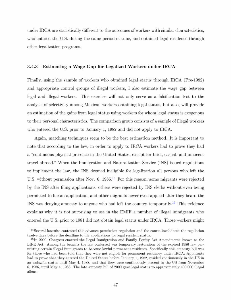
under IRCA are statistically different to the outcomes of workers with similar characteristics,
who entered the U.S. during the same period of time, and obtained legal residence through
other legalization programs.
3.4.3 Estimating a Wage Gap for Legalized Workers under IRCA
Finally, using the sample of workers who obtained legal status through IRCA (Pre-1982)
and appropriate control groups of illegal workers, I also estimate the wage gap between
legal and illegal workers. This exercise will not only serve as a falsification test to the
analysis of selectivity among Mexican workers obtaining legal status, but also, will provide
an estimation of the gains from legal status using workers for whom legal status is exogenous
to their personal characteristics. The comparison group consists of a sample of illegal workers
who entered the U.S. prior to January 1, 1982 and did not apply to IRCA.
Again, matching techniques seem to be the best estimation method. It is important to
note that according to the law, in order to apply to IRCA workers had to prove they had
a “continuous physical presence in the United States, except for brief, casual, and innocent
travel abroad.”When the Immigration and Naturalization Service (INS) issued regulations
to implement the law, the INS deemed ineligible for legalization all persons who left the
U.S. without permission after Nov. 6, 1986.15 For this reason, some migrants were rejected
by the INS after filing applications; others were rejected by INS clerks without even being
permitted to file an application, and other migrants never even applied after they heard the
INS was denying amnesty to anyone who had left the country temporarily.16 This evidence
explains why it is not surprising to see in the EMIF a number of illegal immigrants who
entered the U.S. prior to 1981 did not obtain legal status under IRCA. Those workers might
15Several lawsuits contested this advance-permission regulation and the courts invalidated the regulationtwelve days before the deadline to file applications for legal resident status.16In 2000, Congress enacted the Legal Immigration and Family Equity Act Amendments known as the
LIFE Act. Among the benefits the law conferred was temporary restoration of the expired 1986 law per-mitting certain illegal immigrants to become lawful permanent residents. Specifically this amnesty bill wasfor those who had been told that they were not eligible for permanent residency under IRCA. Applicantshad to prove that they entered the United States before January 1, 1982, resided continuously in the US inan unlawful status until May 4, 1988, and that they were continuously present in the US from November6, 1986, until May 4, 1988. The late amnesty bill of 2000 gave legal status to approximately 400,000 illegalaliens.
47
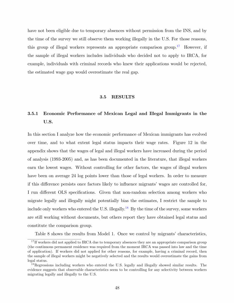
have not been eligible due to temporary absences without permission from the INS, and by
the time of the survey we still observe them working illegally in the U.S. For those reasons,
this group of illegal workers represents an appropriate comparison group.17 However, if
the sample of illegal workers includes individuals who decided not to apply to IRCA, for
example, individuals with criminal records who knew their applications would be rejected,
the estimated wage gap would overestimate the real gap.
3.5 RESULTS
3.5.1 Economic Performance of Mexican Legal and Illegal Immigrants in the
U.S.
In this section I analyze how the economic performance of Mexican immigrants has evolved
over time, and to what extent legal status impacts their wage rates. Figure 12 in the
appendix shows that the wages of legal and illegal workers have increased during the period
of analysis (1993-2005) and, as has been documented in the literature, that illegal workers
earn the lowest wages. Without controlling for other factors, the wages of illegal workers
have been on average 24 log points lower than those of legal workers. In order to measure
if this difference persists once factors likely to influence migrants’wages are controlled for,
I run different OLS specifications. Given that non-random selection among workers who
migrate legally and illegally might potentially bias the estimates, I restrict the sample to
include only workers who entered the U.S. illegally.18 By the time of the survey, some workers
are still working without documents, but others report they have obtained legal status and
constitute the comparison group.
Table 8 shows the results from Model 1. Once we control by migrants’characteristics,
17If workers did not applied to IRCA due to temporary absences they are an appropriate comparison group(the continuous permanent residence was required from the moment IRCA was passed into law and the timeof application). If workers did not applied for other reasons, for example, having a criminal record, thenthe sample of illegal workers might be negatively selected and the results would overestimate the gains fromlegal status.18Regressions including workers who entered the U.S. legally and illegally showed similar results. The
evidence suggests that observable characteristics seem to be controlling for any selectivity between workersmigrating legally and illegally to the U.S.
48
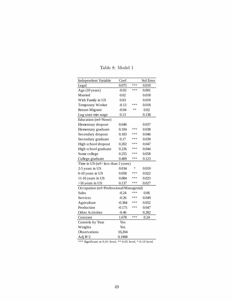
Table 8: Model 1
Independent Variable CoefLegal 0.075 *** 0.019Age (10 years) 0.03 *** 0.001Married 0.02 0.018With Family in US 0.03 0.019Temporary Worker 0.13 *** 0.018Return Migrant 0.04 ** 0.02Log state min wage 0.13 0.138Education (ref=None)Elementary dropout 0.046 0.037Elementary graduate 0.104 *** 0.038Secondary dropout 0.183 *** 0.046Secondary graduate 0.17 *** 0.039High school dropout 0.202 *** 0.047High school graduate 0.226 *** 0.044Some college 0.255 *** 0.058College graduate 0.409 *** 0.123Time in US (ref= less than 2 years)25 years in US 0.034 * 0.019610 years in US 0.058 *** 0.0221116 years in US 0.084 *** 0.023>16 years in US 0.137 *** 0.027
Sales 0.24 *** 0.06Services 0.26 *** 0.049Agriculture 0.384 *** 0.052Production 0.175 *** 0.047Other Activities 0.46 0.282Constant 1.678 *** 0.24Controls by Year YesWeights YesObservations 10,204Adj R^2 0.1908*** Significant at 0.01 level, ** 0.05 level, * 0.10 level.
Std Error
Occupation (ref=Professional/Managerial)
49

legal workers earn wages 7.5 log points higher than illegal workers. The results also show
that wages increase systematically with education and with time in the U.S. Individuals with
2-5 years of experience earn wages 3.4 log points higher than recently arrived workers, while
workers with more than 16 years in the U.S. earn wages 13.7 log points higher than newly
arrived workers.
The results show that the wages of temporary workers are 13 log points lower than those
of permanent workers, a result that can be explained if temporary workers have restricted
mobility and incentives to take jobs that require little investment in education or training.
Finally, the results show that wages of return migrants are 4 log points lower than those
of workers who stay in the U.S. This evidence is in line with the “Disappointment Theory
of Migration”(Herzog and Schottman, 1982) which maintains that people engage in return
migration because they “failed”; they could not find employment or could earn only low wages
at the target location. People move with the intention of settling in the new location but
have limited information before migration and may miscalculate the benefits of migration.
Model 2 estimates the wage gap between legal and illegal workers in six major occupation
groups. The results (Table 9) show that the gap is larger for those working in sales (16 log
points), production (9.9 log points), and services (6.7 log points). For individuals working
in the agricultural sector and as professionals/technicians the wage gap is 2.8 log points and
7.2 log points respectively, however, these differences are not statistically significant.
In Model 3 I estimate the wage gap between legal and illegal workers in twelve more
detailed categories according to their occupation. The results (Table 10) show that the gap
is larger among sales workers (17.7 log points), supervisors in production (16.8 log points),
workers in production (10.9 log points), and workers in the service sector (8.9 log points).
For professionals, technicians, sales managers and agricultural supervisors, the estimated
wage gaps are 16.7, 1.7, 10.3 and 13.6 log points respectively; however, these differences
are not statistically significant. In these occupational categories large standard errors can
be associated to the small number of observations and specifically, to the small number of
illegal workers in these categories. Finally, for laborers in the agricultural sector, workers
providing domestic services, and individuals working as assistants in production the wage
gap is small and not statistically significant (0.5, 2.4 and 1.1 log points respectively).
50

Table 9: Model 2
Independent Variable CoefLegal*Profesional 0.072 0.09Legal*Sales 0.16 ** 0.074Legal*Services 0.067 ** 0.033Legal*Agriculture 0.028 0.031Legal*Production 0.099 *** 0.023Age (10 years) 0.03 *** 0.001Married 0.019 0.018With Family in US 0.032 * 0.019Temporary Worker 0.128 *** 0.018Return Migrant 0.041 ** 0.02Log state min wage 0.134 0.138Education (ref=None)Elementary dropout 0.044 0.036Elementary graduate 0.102 *** 0.038Secondary dropout 0.181 *** 0.046Secondary graduate 0.168 *** 0.039High school dropout 0.2 *** 0.047High school graduate 0.225 *** 0.044Some college 0.253 *** 0.057College graduate 0.409 *** 0.123Time in US (ref= less than 2 years)25 years in US 0.036 * 0.019610 years in US 0.059 *** 0.0221116 years in US 0.084 *** 0.023>16 years in US 0.137 *** 0.027
Sales 0.303 *** 0.09Services 0.257 *** 0.075Agriculture 0.355 *** 0.075Production 0.193 *** 0.073Other Activities 0.499 *** 0.094Constant 1.675 *** 0.245Controls by Year YesWeights YesAdj R^2 0.1912*** Significant at 0.01 level, ** 0.05 level, * 0.10 level.
Std Error
Occupation (ref=Professional/Managerial)
51
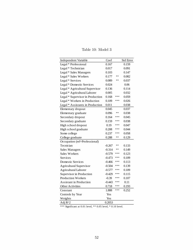
Table 10: Model 3
Independent Variable CoefLegal * Professional 0.167 0.159Legal * Technician 0.017 0.091Legal * Sales Managers 0.103 0.147Legal * Sales Workers 0.177 ** 0.082Legal * Services 0.089 ** 0.037Legal * Domestic Services 0.024 0.06Legal * Agricultural Supervisor 0.136 0.114Legal * Agricultural Laborer 0.005 0.032Legal * Supervisor in Production 0.168 *** 0.059Legal * Workers in Production 0.109 *** 0.026Legal * Assistants in Production 0.011 0.038Elementary dropout 0.045 0.037Elementary graduate 0.096 ** 0.038Secondary dropout 0.164 *** 0.045Secondary graduate 0.159 *** 0.038High school dropout 0.19 *** 0.047High school graduate 0.208 *** 0.044Some college 0.237 *** 0.058College graduate 0.288 ** 0.129Occupation (ref=Professional)Tecnician 0.267 ** 0.133Sales Managers 0.314 ** 0.149Sales Workers 0.579 *** 0.123Services 0.473 *** 0.109Domestic Services 0.466 *** 0.113Agricultural Supervisor 0.504 *** 0.139Agricultural Laborer 0.577 *** 0.109Supervisor in Production 0.429 *** 0.115Production Workers 0.39 *** 0.107Assistant in Production 0.443 *** 0.11Other Activities 0.718 *** 0.193Constant 1.888 *** 0.252Controls by Year YesWeights YesAdj R^2 0.2053*** Significant at 0.01 level, ** 0.05 level, * 0.10 level.
Std Error
52

Table 11: Model 4
Coef CoefAge (10 years) 0.035 *** 0 0.006 0Married 0.056 *** 0.02 0.02 0.02With Family in US 0.036 0.03 0.032 0.02Temporary 0.156 *** 0.02 0.077 *** 0.03Return Migrant 0.087 *** 0.03 0.038 * 0.02Education (ref=None)Elementary dropout 0.046 0.04 0.039 0.04Elementary graduate 0.115 *** 0.04 0.083 * 0.04Secondary dropout 0.184 *** 0.05 0.044 0.05Secondary graduate 0.175 *** 0.04 0.100 ** 0.05High school dropout 0.268 *** 0.05 0.104 * 0.06High school graduate 0.226 *** 0.05 0.126 ** 0.06Some college 0.301 ** 0.08 0.185 *** 0.07College graduate 0.448 *** 0.08 0.341 *** 0.1Time in US (ref= less than 2 years)25 years in US 0.036 0.03 0.035 * 0.02610 years in US 0.07 ** 0.03 0.087 *** 0.021116 years in US 0.094 *** 0.03 0.064 ** 0.03>16 years in US 0.164 *** 0.03 0.085 ** 0.04Occupation (ref=Professional)Technicians 0.254 *** 0.08 0.22 * 0.12Sales Managers 0.163 0.1 0.31 ** 0.15Sales Workers 0.336 *** 0.09 0.5 *** 0.11Services 0.399 *** 0.07 0.38 *** 0.09Domestic Services 0.505 *** 0.08 0.39 *** 0.1Agricultural Supervisor 0.414 *** 0.08 0.4 *** 0.12Agricultural Laborer 0.58 *** 0.07 0.49 *** 0.09Supervisor in Production 0.248 *** 0.08 0.31 *** 0.1Production Workers 0.31 *** 0.07 0.29 *** 0.09Assistant in Production 0.428 *** 0.07 0.36 *** 0.09Constant 1.747 *** 0.27 2.161 *** 0.33Observations 10,341 4,658Adj R^2 0.209 0.158*** Significant at 0.01 level, ** 0.05 level, * 0.10 level.
LEGAL ILLEGALStd Error Std Error
53

In Model 4, to further analyze if the covariates impact differently the wages of legal and
illegal workers, I estimate Model 1 separately for both groups of workers. Table 11 shows
that temporary migrants earn lower wages than their settled counterparts. Illegal temporary
workers earn wages 7.7 log points lower than settled illegal workers, while legal temporary
migrants earn wages 15.6 log points lower than settled legal workers. The results also show
that wages of return migrants are lower than those of workers who stay in the U.S. Legal
return migrants earn wages 8.7 log points lower than legal workers who stay in the U.S., and
illegal return migrants earn wages 3.8 log points lower than the illegal workers who decide to
stay. Finally, wages increase systematically with education and with experience in the U.S.,
two results that are especially strong among legal workers.
Finally, the results from Model 5 (Table 12) show that the wage gap between legal and
illegal workers is 9.0 log points for workers in formal jobs, and is not statistically significant
for workers in informal jobs. This evidence is in line with the idea that firms may be willing
to employ undocumented workers only if the wage is lower so as to compensate for the
additional cost that firms incur when hiring illegal workers. Such costs might include tax
burden, fines and costs of avoiding prosecution, costs that are higher when undocumented
workers have formal jobs.
3.5.2 Testing for Selectivity among Workers obtaining Legal status
In order to evaluate the effect of the potential bias generated if workers with more unobserved
ability are more likely to obtain legal status, I use the 1986 IRCA’s legalization program to
test for selectivity in the population obtaining legal status. Tables 13 and 15 report summary
statistics for the treatment and control groups. For the workers legalized under IRCA Pre-
1982 the control group is a sample of workers who entered the U.S. illegally during the same
period of time and obtained legal status between 1978 and 1985 or between 1992 and 1995.
For the agricultural workers legalized under SAW, the control group is a sample of workers
who entered the U.S. between 1982 and 1986 and received legal status between 1978 and
1985 or between 1992 and 1995.
Table 14 shows the estimated wage gap between workers legalized under IRCA (PRE-
54

Table 12: Model 5
Independent Variable CoefLegal*Formal 0.09 *** 0.02Legal*Informal 0.023 0.016Formal 0.063 *** 0.019Age (10 years) 0.003 *** 0.001Married 0.022 * 0.012With Family in US 0.02 0.016Temporary Worker 0.112 *** 0.013Return Migrant 0.039 *** 0.014Log state min wage 0.141 0.088Education (ref=None)Elementary dropout 0.039 * 0.021Elementary graduate 0.09 *** 0.021Secondary dropout 0.157 *** 0.026Secondary graduate 0.15 *** 0.022High school dropout 0.177 *** 0.029High school graduate 0.186 *** 0.026Some college 0.212 *** 0.04College graduate 0.267 *** 0.047
25 years in US 0.024 0.024610 years in US 0.052 * 0.0231116 years in US 0.075 *** 0.023>16 years in US 0.121 *** 0.025
Technicians 0.363 *** 0.049Sales Managers 0.323 *** 0.064Sales Workers 0.551 *** 0.052Services 0.51 *** 0.044Domestic Services 0.521 *** 0.048Agricultural Supervisor 0.49 *** 0.05Agricultural Laborer 0.655 *** 0.044Supervisor in Production 0.41 *** 0.046Production Workers 0.41 *** 0.043Assistant in Production 0.515 *** 0.046Other Activities 0.446 *** 0.101Constant 1.922 *** 0.159Controls by Year YesWeights YesObservations 10,196Adj R^2 0.1918
Std Error
Occupation (ref=Professional)
Time in US (ref= less than 2 years)
55

Table 13: Summary Statistics: IRCA(PRE-1982) vs Legal Workers
Observations 133 Observations 543 Observations 189Wage 2.09 Wage 2.04 Wage 2.18
Years schooling 6.28 Years schooling 6.18 Years schooling 6.73Age 43.23 Age 43.18 Age 42.56
Year Obtained of Legal Status
1978198519861991
IRCA (PRE1982) 19921995
Year ofArrival
19781981
1982) and the control group. The covariates used are age, age squared, years of schooling,
years of schooling squared, number of years in the U.S., and number of years since legal status
was granted. I also include dummy variables for eleven different occupations, the number of
jobs the migrant has had in the U.S., and dummy variables for temporary workers, workers
with family in the U.S., phase of the survey in which the interview was conducted, and the
state of the U.S. the where the migrant works. Using the methodology provided by Abadie
et al., (2004), I estimate the average treatment effect for the treated (ATT) using bias-
corrected exact matching and estimate the standard errors allowing for heteroskedasticity.19
I use four matches to estimate the conditional variance functions given that four matches
seem to include suffi cient information without matching unlike individuals. Additionally, as
robustness check I also analyze the sensitivity of the estimator to the number of neighbors
used in forming the match estimating the gap with up to five matches. The results show
that there are no significant differences in the earnings of the workers from the treatment
and the control group.
Table 14 also shows estimates of the wage gap using propensity score matching estima-
tion. I use a logit specification to estimate the propensity score; however estimations using a
probit model provide similar results. The estimations are performed following the methodol-
ogy provided by Becker and Ichino (2002). The ATT is estimated using the same covariates
from the specification above and four matching methods: nearest neighbor, stratification,
kernel and radius matching. It is important to mention that the common support condition
19According to Abadie et al., (2004), bootstrapping methods for estimating the variance of matchingestimators do not necessarily give correct results.
56

Table 14: Matching Estimation IRCA (PRE-1982) vs Legal Workers
Propensity Score ATT Std. Err.Stratification matching 0.031 0.036Kernelbased matching 0.037 0.037Nearest neighbor matching 0.006 0.046
Matching Estimator Coef. Std. Err.SATT 1 0.005 0.045SATT 2 0.002 0.041SATT 3 0.008 0.04SATT 4 0.02 0.04SATT 5 0.018 0.04
OLS Coef. Std. Err.OLS 0.019 0.033
Table 15: Summary Statistics IRCA(SAW) vs Legal Workers
Observations 26 Observations 196 Observations 43Wage 1.67 Wage 1.71 Wage 1.91
Years schooling 5.08 Years schooling 5.26 Years schooling 6.3Age 44.46 Age 39.45 Age 39.26
1978198519861991
IRCA (SAW) 19921995
Year ofArrival
19821985
57

Table 16: Matching Estimation IRCA (SAW) vs Legal Workers
Propensity Score ATT Std. Err.Stratification matching 0.013 0.072Radius matching 0.029 0.079Kernelbased matching 0.023 0.083Nearest neighbor matching (RD) 0.001 0.064Matching Estimator Coef. Std. Err.SATT 1 0.014 0.12SATT 2 0.049 0.101SATT 3 0.055 0.1SATT 4 0.017 0.103SATT 5 0.018 0.104
OLS Coef. Std. Err.OLS 0.059 0.082
was imposed and the balancing property was set and satisfied in all the models.20 The results
show no significant differences in the earnings of the treatment and the control group.
Next, I estimate the wage gap between agricultural workers legalized under IRCA SAW
program and the control group. Table 16 shows the estimates obtained using bias-corrected
matching as well as propensity score. The results show that there are no significant differences
in the earnings of the treated and control group.
Based on the previous results, we can conclude that there is no evidence of selectivity
among Mexican workers obtaining legal status. The estimates show that the outcomes of
workers legalized under IRCA are no statistically different than those of workers with sim-
ilar characteristics who obtained permanent residence through other legalization programs.
These results suggest that the observable characteristics of migrants seem to be controlling
for any type of selection among workers obtaining legal status. According to the Bureau of
Consular Affairs during the period of analysis most of the legalizations have been done under
provisions which give priority to those who have immediate relatives and family already in
the U.S. These two methods do not seem to increase the chances of legalization for those
with more unobservable abilities.20The common support test verifies that the overlapping assumption is satisfied and the balancing property
verifies that the covariates are balanced within each block, that is, that the difference between the averageof the covariates for the treatment and control groups within each block is small.
58

Table 17: Summary Statistics Legal (IRCA PRE-1982) and Illegal Workers
Observations 543Wage 2.04Years schooling 6.18Age 43.18
Observations 86Wage 1.75Years schooling 5.44Age 41.8
Year ofArrival
19781981
Year ofArrival
19781981
Legal Workers (IRCA PRE1982)
Illegal Workers
3.5.3 Estimating a Wage Gap for Legalized Workers under IRCA
Finally, using again matching estimators for the sample of workers who obtained legal status
through IRCA (PRE-1982), and a sample of illegal workers who entered prior to January 1,
1982 and did not apply to IRCA, I estimate the wage gap between legal and illegal workers.
As mentioned before, this is an appropriate control group since their legal status seems to
be exogenous to personal characteristics; a number of migrants were not eligible for IRCA
due to temporary absences from the U.S. However, if the sample of illegal workers includes
individuals who decided not to apply to IRCA, for example, individuals with criminal records
who knew their applications would be rejected, the wage gap would be overestimated, and
the results obtained would represent an upper bound for the real gap. Table 17 reports
summary statistics for the treatment and control groups.
Table 18 shows the estimated wage gap. The covariates used are age, age squared, years
of schooling, years of schooling squared, and number of years in the U.S. I also include
dummy variables for eleven different occupations, the number of jobs that migrants have
had in the U.S., and dummy variables for temporary workers, workers with family in the
U.S., phase of the survey in which the interview was conducted, and the state of the U.S.
where migrants work.
The ATT estimated using bias-corrected exact matching shows a gap of 15.5 log points
while matching using different number of covariate matches show a statistically significant
59

Table 18: Matching Estimation IRCA (PRE-1982) vs Illegal Workers
Propensity Score ATT Std. Err.Stratification matching 0.138 0.094Radius matching 0.131 0.099Kernelbased matching 0.177 0.089Nearest neighbor matching 0.115 0.115
Matching Estimator Coef. Std. Err.SATT 1 0.155 ** 0.079SATT 3 0.135 * 0.08SATT 5 0.135 * 0.079SATT 7 0.136 * 0.078SATT 10 0.147 * 0.078OLS Coef. Std. Err.OLS 0.097 0.067
wage gap between 13.5 and 14.7 log points. Table 18 also shows estimates of the wage gap
using propensity score matching estimation using the same covariates from the specification
above. The ATT estimated using nearest neighbor matching shows a gap of 11.5 log points,
stratification matching a gap of 13.8 log points, kernel matching a gap of 17.7 log points,
and radius matching a gap of 13.1 log points.
Based on the previous results, we can conclude that once I control for different individual
characteristics, legal workers earn wages 12 to 17 log points higher than those of illegal
workers. This gap seems to be robust since different matching techniques provided similar
results, and unbiased, since legal status is granted based on date of arrival and is exogenous
to migrants’characteristics.
3.6 CONCLUSIONS
I estimate the effect of legal status on the wages of Mexican immigrants in the U.S. using
Mexico’s Survey of Migration to the Northern Border. I control for possible selection bi-
ases and test for selectivity in the population obtaining legal status using the 1986 IRCA’s
60
legalization program along with matching estimation techniques.
The results show that legal workers earn higher wages than illegal workers, especially
those working in the production and service sectors. Controlling for observable characteristics
and occupation decreases the wage differential; however, we still observe a significant wage
gap. Moreover, the results show discrimination against illegal workers does not seem to
explain the wage differences between legal and illegal workers, since the wage gap is only
observed among workers in specific occupations. Finally, the results show that the wage
gap is larger among individuals working in “formal”jobs. While it is true that some illegal
workers are paid off the books, an important number of undocumented workers get formal
jobs using false social security numbers. The evidence is in line with the idea that firms may
hire undocumented workers in formal jobs if the wage is lower so as to compensate for the
additional expenses that firms incur from hiring undocumented workers (e.g. tax burden,
fines or costs of avoiding prosecution).
The results also show that temporary migrants earn lower wages than their settled coun-
terparts, a finding that can be explained if temporary workers have restricted mobility and
incentives to take jobs that require little investment in education or training. Additionally,
I find that return migrants earn lower wages than those of workers who decide to stay in the
U.S. This evidence is in line with the “Disappointment Theory of Migration”that maintains
that people engage in return migration because they “failed”; they could not find employ-
ment or could earn only low wages at the target location. Finally, it is interesting to note
that wages increase systematically with education and with experience in the U.S.; these
results that are especially strong among legal workers.
I test for selectivity in the population obtaining legal status using the 1986 IRCA’s
legalization program, which provides us with a legalization procedure that is exogenous to
migrants’characteristics. Using matching and propensity score estimation, I find no evidence
of selectivity among Mexican workers obtaining legal status. The estimations show that the
outcomes of workers legalized under IRCA are no statistically different than those of workers
with similar characteristics who obtained permanent residence through other channels. These
results suggest that the observable characteristics of migrants seem to be controlling for any
type of selectivity among workers obtaining legal status.
61

Finally, I estimate a wage gap between workers legalized under IRCA and an appropri-
ate group of illegal workers. The results show that once I control for different individual
characteristics, there is a significant gap in the wages of legal and illegal workers of 12 to 19
percent. This gap seems to be robust since different matching techniques provided similar
results, and unbiased, since legal status is granted based on date of arrival and is exogenous
to migrants’characteristics.
Given the large number of Mexican migrants working in the U.S. labor market, a better
understanding of their characteristics and job market outcomes is an issue of great relevance
for Mexico and the U.S. A deeper knowledge of the benefits of having legal status and the
characteristics of those obtaining legal status can provide policymakers with useful informa-
tion to better estimate, not only the implications of the current immigration policy, but also
the impact that future changes to the U.S. immigration policy could have on the U.S. labor
market.
62

4.0 WHO STAYS AND WHO GOES BACK HOME? EVIDENCE FROM
MEXICAN IMMIGRANTS IN THE U.S.
4.1 INTRODUCTION
To better understand the dynamics of the immigrant flow, it is essential to analyze the
characteristics of return migrants. Return migration is an important phenomenon that has
received little attention in the literature even though it involves a large share of migrants
and has large social, economic, and cultural impacts on both, the home and host countries.
If long-term settlement is not a random process, return migration will not only affect the
composition of the immigrant population and their use of social services in the host country,
but also the economic development in the home country through remittances and investment.
In this paper I study return migration of Mexican migrants in the United States. Borjas
and Bratsberg (1996) show that the return migration process accentuates the type of selection
that originally characterized the immigrant flow. According to their theoretical prediction,
if the immigrant flow is positively selected, the outmigrants should be less skilled than the
immigrants who remain in the United States (U.S.). If the immigrant flow is negatively
selected, the outmigrants will be more skilled than the immigrants who remain in the U.S.
In this paper I test Borjas and Bratsberg’s prediction. I use data from the Survey
of Migration to the Northern Border (EMIF) together with a selection model to infer the
unobservable skills of Mexican immigrants and the unexpected component of their earnings
in the U.S. I test for differences in the observable skills, unobservable skills, and uncertainty
component associated with U.S. earnings of return migrants and migrants who stay in the
U.S.
The results show that immigrants are negatively selected relative to the Mexican popula-
63

tion. Consistent with Borjas and Bratsberg’s prediction, return migrants are relatively more
skilled than the typical immigrant. Moreover, workers who face more negative unexpected
conditions in the U.S. are those who find it optimal to return to Mexico.
4.2 LITERATURE REVIEW
Despite the practical importance of return migration, little is known about the selection
process guiding the outmigration decision of the foreign born. An important body of litera-
ture has considered return migration as a cost-benefit decision, where individuals decide to
stay or return in order to maximize their expected lifetime earnings. Sjaastad (1962) pro-
vides a theoretical framework for the decision to migrate where individuals calculate their
present discounted value of expected returns in different locations, and migration occurs if
the returns in a potential destination, net of migration costs, are larger than the returns in
their home country.
According to this view, immigrants originally move in response to higher wages in the
host country, which they expect to yield higher lifetime earnings. In the absence of a re-
duction in the binational wage differential, return migration should only occur if a migrant’s
expectations for higher earnings are not met, if wages are lower than expected, or if the
psychic costs of moving are higher than anticipated. In this sense, return migrants are view
as “failures”, what Duleep (1994) calls “mistaken migrants”, and Herzog and Schottman
(1982) call “disappointed migrants”.
However, these predictions are often not compatible with the empirical evidence. Some
authors have provided explanations to rationalize the fact that migrants return, despite
persistently higher wages in the host country. Djajic and Milbourne (1988) assume that
different preferences for consuming at home and at the destination may be responsible for
temporary migration. Dustmann (1995, 1997) shows that high purchasing power of the host
country currency at home, and higher returns to human capital in the home economy, are
some of the motives behind return migration. Mesnard (2004) analyzes how capital market
imperfections influence return migration and shows that return migration may be one way
64

to overcome capital constraints.
An alternative view of return migration is known as the "Target Income Theory of
Migration”(Stark 1991, Borjas 1994, Hill 1987, Lindstrom 1996, Massey et al. 1993). This
theory states that immigrants move to accumulate savings to invest in their home countries.
That is, migrants plan to stay in the host country as long as is required to accumulate enough
savings to reach a particular level of income. Once reaching the target, they return to their
place of origin. This theory assumes that immigrants have a strong preference for remaining
in their home country and migrate due to limited wage opportunities at home.
Borjas and Bratsberg (1996) present a model that incorporates both theories of return
migration. First, return migration may have been planned as part of an optimal life-cycle
residential location sequence, where some immigrants migrate to the U.S. for a few years, ac-
cumulate financial resources or other types of capital, and then return to the source country.
Alternatively, return migration might occur if immigrants based their initial migration deci-
sion on erroneous information about economic opportunities in the U.S. This model predicts
that return migration accentuates the type of selection that originally characterized the im-
migrant flow. The authors confirm their theoretical predictions by calculating outmigration
rates for immigrants from 70 source countries using data from the 1980 U.S. Census.
Two studies that empirically analyze the selection process guiding return migration are
Borjas (1989) and Jasso and Rosenzweig (1988). In the Borjas’ study, return migration
is inferred from sample attrition in a longitudinal data set of foreign born scientists and
engineers. He finds that the least successful scientists and engineers are most likely to drop
out from the sample, and concludes that the outmigration process is one in which "failures"
leave the U.S. In contrast, Jasso and Rosenzweig observe the naturalization decision of
immigrants, and infer that those who do not naturalize are most likely to leave the country.
In their study, it is the most skilled workers who do not naturalize, and are most likely to
be outmigrants.
65

4.3 BORJAS AND BRATSBERG’S MODEL
Individuals in the home country (country 0) consider the possibility of migrating, either
temporarily or permanently to the host country (country 1). The log earnings distributions
in the source and home countries are given by:
w0 = µ0 + υ
w1 = µ1 + λυ + ε1
where µ0 is the mean log income in the source country, and µ1 is the mean income that
would be observed if all persons in the source country (Mexico) migrate to the host country
(U.S.). The parameter λ represents the rate of return to skills in the U.S. relative to that in
Mexico. The parameter υ reflects ability or skills that are transferable across countries and is
assumed to be known to the individual. The parameter ε1 reflects an uncertainty component
due to misinformation or luck in U.S. earnings, and is assumed to remain unknown unless
the individual migrates to the U.S. The random variables υ and ε1 measure deviations from
mean incomes, have zero means and finite variances, and are assumed to be independent.
Workers in Mexico can migrate temporarily to the U.S. followed by a permanent return
to Mexico. The log earnings associated with this alternative are given by:
w10 = πw1 + (1− π)(w0 + k)
where π and k represent the time that the individual stays in the U.S. and the gain to a
temporary stay. Both parameters are constant among individuals.
Assuming risk neutrality, a person migrates to the U.S. if the expected value of the max-
imum between the wage from migrating permanently and temporarily to the U.S., exceeds
the wage in Mexico net of migration costs:
E [max {w1 −M,w10 −M −R}] > w0,
66

where M and R are time equivalent measures of migration cost to the U.S. and remigration
costs to Mexico.1
Individuals who migrate to the U.S. will return to Mexico if they migrated in the first
place, and if the actual available income in the U.S. is lower than the potential income in
Mexico.
E [max {w1 −M,w10 −M −R}] > w0
and
max[w0 −R,w10 −R] > w1.
Combining the last two expressions it can be found that an individual will stay in Mexico
if
υ(λ− 1) ≤ (µ0 − µ1 + κ) +M +R + κ
π;
will migrate to United States if:
υ(λ− 1) > (µ0 − µ1 + κ) +M +R + κ
π,
and will return to Mexico if:
(µ0 − µ1 + κ) +M +R + κ
π< υ(λ− 1) < (µ0 − µ1 + κ)− R
1− π − ε1.
Figure 3 shows the skill sorting in human capital model when immigrants are positively
selected (λ > 1) and negatively selected (λ < 1) when there is not uncertainty in the mi-
gration decision. If the immigrant flow is positively selected, the outmigrants should be
less skilled than the immigrants who remain in the United States. If the immigrant flow is
negatively selected, the outmigrants will be more skilled than the immigrants who remain
in the U.S.
Return migration can also arise as immigrants attempt to correct mistakes in the initial
immigration decision. The introduction of uncertainty in U.S. economic opportunities does
not alter the type of selection that characterizes the immigrant flow because individuals
1According to Borjas and Bratsberg the decision is made by comparing the maximum of the expectationof the wages if migration is permanent or temporary and the wage in the source country net of migrationcosts: max[Ew1 −M,Ew10 −M −R] > w0. However these differences do not change the predictions of themodel.
67

Figure 3: Skill Sorting in Human Capital Model
68
migrate in order to maximize their expected value of income. After arrival in the U.S., the
immigrant makes a random draw from the g(ε) density, and reconsiders the profitability of
his original decision. The decision of whether to return to Mexico depends on whether the
draw is favorable or unfavorable. Figure 4 shows that only those persons who have relatively
unfavorable draws become return migrants.
The skill composition of the return migration flow in this model is identical to the sorting
implied by the human capital model. In particular,
E(υ| Migrate and Stay) > E(υ| Migrate and Return), for λ > 1
and
E(υ| Migrate and Stay) < E(υ| Migrate and Return), for λ < 1.
If λ > 1, return migrants are relatively unskilled workers (selected from a skilled im-
migrant flow), while if λ < 1, return migrants are relatively skilled workers (selected from
an unskilled immigrant flow). As before, return migration accentuates the selection that
characterizes the original immigration. Figure 4 shows that the random variable υ for return
migrants is truncated from above when λ > 1, and υ is truncated from below when λ < 1.
4.4 DATA
Data on Mexican population is from the 1995 Mexican population and dwelling count, and
the 2000 Mexican Census. Data on Mexican migration comes from the Survey of Migration to
the Northern Border (EMIF), a cross-sectional survey conducted ten times between 1993 and
2005 that samples the flows of migrants between Mexico and the U.S. in the northern border
region of Mexico.2 The EMIF contains information of wages in Mexico prior migration, wages
in the U.S., as well as many other characteristics such as age and education. Additionally,
in the survey it is possible to identify workers by legal status and return migrants.
2The survey is conducted in eight Mexican border cities. Within each city, individuals are sampled atdifferent locations including bus stations, airports, ports of entry and Mexican customs inspection stations.
69

Figure 4: Skill Sorting Uncertainty Model
70
I impose some sample restrictions. I limit the sample to workers who migrated to the
U.S. after 1992, who were working in Mexico prior migration, and report their wages. I
also restrict the sample to include migrants who worked at least 30 days in the U.S. and
report their wages, and who were surveyed by the EMIF within the first three years of
U.S. residency. "Return migrants" are workers returning to Mexico who plan to settle there
permanently and have no intention to return to work in the U.S. in the near future. Migrants
who "Stay in the U.S." are workers who are visiting Mexico but will return to work either
temporarily or permanently to the U.S.
Hourly wages in the U.S. are estimated using migrants’ information on last month’s
earnings, number of hours worked per day and number of days worked per week.3 A selection
issue can arise if workers with different characteristics are more or less likely to cross the
Mexico-U.S. border, since they might appear in the sample at different rates.4 In order to
address this problem, using the number of times that each worker has entered and exited
the U.S., I estimate their probability of being observed in the sample and construct a set of
weights using the inverse of that probability.
Table 19 provides descriptive statistics for all immigrants, return migrants, migrants who
stay in the U.S. Immigrants have on average 6.15 years of schooling, their average wage in
the U.S. is $5.75 per hour (in 2001 U.S. dollars), and their wage in Mexico prior migration
was $1.65 per hour (in 2001 U.S. dollars). It is important to note that while 12.9 percent of
the immigrants entered the U.S. legally, by the time of the survey 27.7 percent are authorized
to work in the U.S. Return migrants are slightly less educated; earn lower wages in the U.S.,
but report higher wages in Mexico prior migration.
3For workers reporting daily, quarterly or monthly wages in Mexico, hourly wages are estimated assumingthey work eight hours per day, six days per week and 4.33 weeks per month.
4For example, illegal workers might be more likely to cross back and forth if they earn low wages in theUS since the opportunity cost of being caught is lower; or if they earn high wages, and can afford to paysmugglers’fees more often.
71

Table 19: Summary Statistics Return Migrants and Migrants who Stay in the U.S.
Mean SD Mean SD Mean SDCharacteristicsLegal at Survey 27.7% 0.45 23.9% 0.43 40.0% 0.49Legal at Entry 12.9% 0.33 11.4% 0.32 17.5% 0.38Return Migrant 75.7% 0.43 100.0% 0.00 0.0% 0.00Age 33.2 10.5 33.2 10.4 33.4 10.7Married 69.2% 0.46 70.1% 0.46 66.8% 0.47Family in US 77.7% 0.42 76.7% 0.42 80.5% 0.40Female 2.0% 0.14 1.6% 0.13 3.2% 0.18Years of schooling 6.15 3.40 6.12 3.34 6.25 3.61No education 8.3% 0.28 7.9% 0.27 9.5% 0.29Elementary dropout (<6y) 25.8% 0.44 25.9% 0.44 25.8% 0.44Elementary graduate (6y) 28.3% 0.45 28.8% 0.45 26.4% 0.44Secondary dropout (78y) 8.4% 0.28 8.5% 0.28 8.2% 0.27Secondary graduate (9y) 18.4% 0.39 18.8% 0.39 16.9% 0.37High school dropout (1011y) 3.8% 0.19 3.7% 0.19 4.1% 0.20High school graduate (12y) 4.8% 0.21 4.4% 0.21 6.1% 0.24Some College (1315) 1.2% 0.11 1.0% 0.10 1.9% 0.14College graduate (>=16y) 0.9% 0.10 0.9% 0.09 1.2% 0.11Earnings
Wage US15.75 4.59 5.68 4.81 6.00 3.91
Wage Mexico11.65 4.26 1.71 4.54 1.48 3.30
Occupation in USProfessional/Technicians 1.8% 0.13 1.5% 0.12 3.0% 0.17Sales 1.7% 0.13 1.6% 0.12 2.1% 0.14Services 21.3% 0.41 21.5% 0.41 19.9% 0.40Agricultural 34.5% 0.48 35.2% 0.48 32.8% 0.47Production 40.6% 0.49 40.2% 0.49 42.2% 0.49Other Activities 0.1% 0.03 0.1% 0.04 0.0% 0.00Observations 5,538 4,144 1,3941In 2001 US Dollars. Wages in Mexico prior migration.
All Immigrants Return Migrants Migrants Stay in US
72

4.5 EMPIRICAL SPECIFICATION
I will use Borjas and Bratsberg’s selection model along with data of Mexican immigrants and
the Mexican population to infer the unobservable transferable skills of immigrants and the
unexpected component of their earnings in the U.S. To determine the type of selection process
guiding the outmigration decision of Mexican immigrants, I test for significant differences in
the unobserved skills and the uncertainty component of return migrants and migrants who
stay in the U.S. The wage equations in Mexico and the U.S. are given by:
w0i = α0 + β0Xi + υi (4.1)
and
w1i = α1 + β1Xi + λυi + ε1i (4.2)
where w0i is the logarithm of the hourly wage in Mexico of individual i, w1i is the logarithm of
the hourly wage in the U.S. of individual i, Xi is a set of individual observable characteristics
such as age, years of schooling, gender, marital status, and state; υi represents unobserved
workers’transferable skills, λ is the rate of return to skills in the U.S. relative to Mexico,
and ε1i is a random shock.
Step 1
Using equation (4.1) and data from the 1995 Mexican Population and Dwelling Count
and the 2000 Mexican Census, I estimate the returns to observable characteristics for the
Mexican population. I restrict the sample to include individuals who work, report their wage
and are aged 16 to 65. I run this regression separately for year 1995 and 2000, and obtain a
set of coeffi cients for each year.
Step 2
For the sample of Mexican immigrants surveyed by EMIF, I find the returns to observable
and unobservable characteristics in the Mexican labor market. I use information of wages in
Mexico prior migration (w0i), a set of personal characteristics (Xi), and the rate of return
to observable characteristics in the Mexican labor market (the coeffi cients obtained in the
73

previous step). The estimated unobservable transferable skills (υi) for Mexican immigrants
are given by:
υi = w0i − (α0 + β0Xi).
For workers who entered the U.S. between 1993 and 1997 I use the coeffi cients obtained
in the regression for the Mexican population in 1995. For workers who entered after 1997 I
use the coeffi cients obtained in the regression with data from 2000.
Step 3
The next step is to find the rate of return to observable (β1) and unobservable charac-
teristics (λ) in the U.S. labor market for the sample of immigrants. Using information of
migrants’wages in the U.S. (w1i), a set of individual observable characteristics (Xi), and
their unobservable skills (υi), I estimate the following wage regression:
w1i = α1 + β1Xi + λυi + ε1i. (4.3)
The coeffi cient associated with υi is the rate of returns to skills in the U.S. relative to
Mexico (λ), and the residuals obtained (ε1i) can be interpreted as the uncertainty component
associated with immigrants’U.S. earnings
ε1i = w1i − α1 − β1Xi − λυi.
I test for significant differences in the transferable skills (υi) and the uncertainty compo-
nent (ε1i) between return migrants and migrants who decide to stay in the U.S. Moreover,
I test if the selection process is different between workers migrating legally and illegally to
the U.S.
Alternatively, if we change Borjas and Bratsberg’s model, and we allow for shocks in the
Mexican labor market equation (4.1) becomes:
w0i = α0 + β0Xi + υi + ε0i. (4.4)
74

If we assume that the unobservable skills υi are uncorrelated with workers’observable
characteristics Xi, and that the estimated unobservable skills υi are uncorrelated with the
error term ε0i, in step 2 we will only be able to estimate υi + ε0i instead of υi with
υi + ε0i = w0i − (α0 + β0Xi).
Therefore, the equation (4.3) for the U.S. labor market becomes
w1i = α1 + β1Xi + λχi + ui (4.5)
where
χi = υi + ε0i and ui = ε1i − λε0i.
In this setting, since χi and ui are correlated, the results will suffer of attenuation bias.
If λ is positive, λ will tend to underestimate λ, if λ is negative, λ will overestimate the rate
of returns to skills in the U.S. relative to Mexico.
One caveat of this study is that it only includes immigrants who entered the U.S. since
1992 due to data availability. While this analysis can be extended to analyze future waves
of immigrants, the selectivity of previous cohorts cannot be determined. Estimates suggest
that almost half of the Mexican workers migrating to the U.S. return to Mexico within
twelve months, therefore, analyzing the behavior of immigrants who entered the U.S. during
a 10 year window, provide a representative picture of the selection process guiding return
migration.
75

Table 20: Education and Earnings of Immigrants and Mexican Population
1995 2000Years of schooling 8.77 8.94 6.15
(4.22) (4.44) (3.40)
Wage Mexico1 2.19 2.12 1.65(3.51) (9.01) (4.26)
Wage U.S.1 5.75 (4.59)
Observations 61,118 355,054 5,538
Mexican Population ImmigrantsEMIF
4.6 RESULTS
4.6.1 Selectivity of Mexican Workers Migrating to the U.S.
The results show that the immigrant flow of Mexican workers is negatively selected in terms
of their observable and unobservable skills. Table 20 shows that the number of years of
education for immigrants is significantly lower than the average years of schooling for the
Mexican population. While the average educational attainment in Mexico was 8.77 in 1995
and 8.94 years in 2000, the average years of schooling among Mexican workers who migrated
between 1992 and 2005 is only 6.15 years. Additionally, Mexican workers are negatively
selected based on their unobservable transferable skills. Table 21 shows that while the
average unobserved skills is zero for the Mexican population, the average skills for Mexican
immigrants is -0.248 and this difference is statistically significant.
The rate of return to unobserved transferable skills in the U.S. relative to Mexico is
estimated to be 0.085. Since the rate of return to skills is higher in Mexico than in the
U.S., workers with more skills have little incentive to migrate to the U.S. Additionally, the
estimated rate of return to one year of schooling is βyschool0 = 0.10 in Mexico, and βyschool1 =
0.03 in U.S.
Table 20 also shows that the wages of immigrants in Mexico (prior migration) are lower
than the average wages for the Mexican population. Those differences in wages can be ex-
76

Table 21: Unobserved Skills of Immigrants and Mexican Population
ImmigrantsEMIF1
MexicanPopulation1 Difference2
0.248 0.00 0.248***
(0.91) (0.00) (0.002)1Standard deviations in parenthesis. 2Standard error in parenthesis.*** Significant at 0.01 level.
Unobservedtransferable skills
plained due to different observable characteristics like age or education, or due to differences
in the unobservable skills. In order to test the source of the wage differential, I estimate the
wages that immigrants would earn if they had similar characteristics to the average Mexican
resident (eliminate differences in terms of observable characteristics). The results show that
the differences in wages are mainly due to differences in unobservable skills. Figure 5 shows
the average wages for the Mexican population, the wages that migrants earned in Mexico,
and the wages that those migrants would earn if they had characteristics similar to the
ones of the average Mexican resident. Even if we compensate migrants for their differences
in observable characteristics, their wages are still significantly lower than the wages of the
Mexican population.
4.6.2 Selectivity of Return Migration
Table 22 shows the years of education and the unobserved skills for return migrants and
migrants who stay in the U.S. Migrants who stay are slightly more educated; however, the
difference in years of schooling is not statistically significant. For both groups of workers the
value of their unobserved skills is negative, which implies that both groups of migrants are
negatively selected relative to the Mexican population. However, the value of the unobserved
skills is higher (less negative) among return migrants, which implies that return migration
intensifies the negative selection that originally characterized the immigrant flow.
Table 22 also shows the uncertainty component (ε). The results show that migrants who
decide to return to Mexico are those with lower values of ε. Therefore, workers who faced
77

Figure 5: Wages in Mexico: Immigrants prior Migration and Mexican Population
Table 22: Education, Unobserved Skills and Uncertainty Component of Return Migrants
Immigrants EMIFReturn Migrants1 Migrants Stay1 Difference2
Years of schooling 6.116 6.252 0.137(3.34) (3.61) (0.17)
Unobserved skills ÝcÞ 0.182 0.446 0.264DDD
(0.85) (1.07) (0.05)Uncertainty component ÝPÞ 0.025 0.078 0.103DDD
(0.65) (0.59) (0.03)US earnings ÝVc + PÞ 0.041 0.040 0.081DDD
(0.66) (0.60) (0.03)Observations 4,144 1,3941Standard deviations in parenthesis. 2Standard errors in parenthesis.DDDSignificant at 0.01 level.
78

unfavorable conditions or bad luck in the U.S. are more likely to become return migrants.
Finally, since the return migrants are more skilled (highest υ’s) than the ones who stay, and
the ones who faced unfavorable conditions or bad luck (lowest ε’s) it is not evident if the
earnings associated to unobserved skills and the uncertainty component of those who return
home are higher or lower than those who stay in the U.S.
(λυ + ε|stay) ≶ (λυ + ε|return)
Table 22 shows that the U.S. wages (λυ+ ε) of return migrants are lower than the wages
of those who stay in the U.S., therefore, the uncertainty effect dominates.
4.6.3 Differences among Legal and Illegal Workers
Previous studies analyzing the selectivity of Mexican immigrants to the U.S. have pointed out
that the type of selection is determined by workers’migration costs. Chiquiar and Hanson
(2005) construct a model that incorporates migration costs and find that the selection of
workers from Mexico depends on the size of migration costs and how they vary with skills. If
illegal workers face higher migration costs than legal workers, the type of selectivity observed
among both groups of workers might differ. Gonzalez (2011) finds evidence of intermediate
selection among Mexican immigrants in terms of education; however, this selectivity becomes
more negative when he analyzes the selectivity of illegal workers. In light of this evidence, it
becomes a relevant issue to study the type of selection guiding the return migration decision
of legal and illegal workers. In this section I test for differences in the observable and
unobservable skills, as well as in the uncertainty component associated with U.S. earnings
of return migrants and migrants who stay by legal status. In this section legal status is
considered at the moment of entry. While most of the workers have the same legal status
during their time in the U.S., some of them obtained legal status after entering illegally and
others overstay their work permits and work undocumented at the time of the survey.
Table 23 shows the differences in the characteristics of legal and illegal workers. Illegal
workers are less educated and have higher unobserved transferable skills than legal workers.
79

Table 23: Education, Unobserved Skills and Uncertainty Component by Legal Status
Immigrants EMIFLegal1 Illegal1 Difference2
Years of schooling 6.811 6.054 0.757DDD
(3.97) (3.30) (0.25)Unobserved transferable skills ÝcÞ 0.346 0.232 0.113D
(0.92) (0.91) (0.06)Uncertainty component ÝPÞ 0.016 0.002 0.018
(0.67) (0.63) (0.04)Observations 572 5,0181Standard deviations in parenthesis. 2Standard errors in parenthesis.DDDSignificant at 0.01 level, Dsignificant at 0.1 level.
With respect to the uncertainty component, there are not significant differences between
legal and illegal workers.5
Table 24 reports years of schooling and unobserved skills for return migrants and migrants
who stay in the U.S. by legal status. Migrants who stay in the U.S. are slightly more educated;
however, the difference in years of schooling is not statistically significant for legal and illegal
workers. For legal workers, the value of the unobserved skills is negative, and there are not
significant differences between return migrants and migrants who stay. For illegal workers
the value of the unobserved skills is also negative, but is higher (less negative) among return
migrants. These results suggest that return migration accentuates the negative selection
that originally characterized the immigrant flow in terms of unobservable skills, particularly
among illegal workers. Illegal return migrants have more unobservable skills than the illegal
workers who stay in the U.S.
Table 25 shows the value of the uncertainty component ε. Among legal and illegal
workers, return migrants are those with lower values of ε. Workers who faced unfavorable
conditions or bad luck in the U.S. return to Mexico, and that effect is stronger among legal
workers.
5The proportion of workers who entered the U.S. illegally is 89.8 percent. The only reference is reportedby Passel, J. (2006) who reports that in recent years about 80 to 85 percent of the immigrants coming fromMexico entered the US undocumented.
80

Table 24: Education and Unobserved Skills of Return Migrants by Legal Status
Education Unobserved skills ÝcÞ
Legal Illegal Legal IllegalReturn Migrants 6.748 6.035 0.284 0.169Standard Deviation (3.77) (3.27) (0.84) (0.85)Observations 382 3758 382 3758Stay in US 6.948 6.105 0.470 0.441Standard Deviation (4.38) (3.41) (1.06) (1.08)Observations 187 1209 187 1209Difference 0.201 0.070 0.186 0.272DDD
Standard Error (0.620) (0.162) (0.132) (0.048)DDDSignificant at 0.01 level, Dsignificant at 0.1 level.
Table 25: Uncertainty Component and U.S. Earnings of Return Migrants by Legal Status
Uncertainty component ÝPÞ US earnings ÝVc + PÞ
Legal Illegal Legal IllegalReturn Migrants 0.052 0.022 0.076 0.036Standard Deviation (0.679) (0.649) (0.687) (0.655)Observations 382 3739 382 3739Stay in US 0.151 0.063 0.111 0.025Standard Deviation (0.628) (0.584) (0.636) (0.588)Observations 187 1203 187 1203Difference 0.203DD 0.084DDD 0.187DD 0.061DD
Standard Error (0.090) (0.029) (0.092) (0.029)DDDSignificant at 0.01 level, DDsignificant at 0.05 level.
81

Finally, Table 25 shows that the U.S. wages (λυ + ε) of return migrants are lower than
the wages of those who stay in the U.S. for both groups of workers. The results show that the
uncertainty effect dominates; even though return migrants have higher unobservable skills,
they earn lower wages in the U.S. because they also face more adverse conditions. This result
is especially strong among legal workers.
4.7 CONCLUSIONS
This paper examines the return migration behavior of Mexican migrants in the United States.
I test Borjas and Bratsberg’s (1996) theoretical prediction that the return migration process
accentuates the type of selection that originally characterized the immigrant flow. According
to their model, if the immigrant flow is positively selected, the outmigrants should be less
skilled than the immigrants who remain in the U.S. If the immigrant flow is negatively
selected, return migrants will be more skilled than the immigrants who remain in the U.S.
I use the Survey of Migration to the Northern Border together with a selection model
to infer the unobservable skills and the unexpected component of their earnings in the U.S.
of return migrants and migrants who stay in the U.S. The results show that the immigrant
flow of Mexican workers is negatively selected, workers migrating from Mexico to the U.S.
are those with lower observable and unobservable skills. In terms of earnings in Mexico, the
wages of immigrants are lower than the average wage of Mexican residents. While part of
the wage differential is explained by differences in their observable characteristics, most of
the difference is associated to differences in their unobservable skills.
The evidence is consistent with Borjas and Bratsberg’s prediction, return migration
accentuates the negative selection that originally characterized the Mexican immigrant flow.
Return migrants are relatively more skilled than the typical immigrant; workers with the
lowest unobservable skills are the ones who find optimal to reside in the United States.
Additionally, I test how U.S. opportunities impact the return migration decision of immigrant
workers. The results show that return migrants are workers who earned lower wages and
faced more unfavorable conditions in the U.S.
82

The large increase in the proportion of Mexican immigrants who enter the U.S. illegally;
the increases in migration costs faced by illegal workers due to tighter border enforcement,
and the fact that the type of selection that characterizes the immigrant flow depends on the
size of migration costs, heighten the importance of studying the type of selection determining
the return migration decision of legal and illegal workers.
The evidence shows that return migration accentuates the negative selection that charac-
terizes the immigrant flow in terms of unobservable skills, particularly among illegal workers.
Illegal workers with the highest skill levels are the ones who find it optimal to return to Mex-
ico. In terms of the unexpected component of U.S. earnings, return migrants faced more
unfavorable conditions in the United States, and that effect is stronger among legal workers.
There are two important caveats to these results. First, this study only includes immi-
grants who entered the U.S. between 1993 and 2005. While this analysis can be extended
to analyze future waves of immigrants, the selectivity of previous cohorts cannot be deter-
mined. Second, I analyze the selectivity of return migration using legal status at the time
of entry. However, an important number of immigrants who enter the U.S. illegally obtain
legal status once in the U.S., and also, a number of legal workers overstay and work without
documents. As a further extension, the selectivity among workers who change their legal
status after entry should be considered.
83

5.0 APPENDIX
5.1 APPENDIX TO CHAPTER 1
84

Table 26: Effect of an Amnesty with and without Tax Adjustment
Baseline NoTaxAdj
Tax Adj Baseline NoTaxAdj
Tax Adj
Vacancy/Unemployment ratio 0.720 0.124 0.137 0.717 0.117 0.134Probability filling a vacancy 0.456 0.038 0.042 0.457 0.036 0.041Probability finding a job 0.328 0.034 0.038 0.327 0.032 0.037Unemployment rate legal 9.39% 0.97% 1.09% 9.41% 0.92% 1.07%Unemployment rate illegal 16.10% 1.53% 1.71% 16.14% 1.44% 1.69%Wage legal 0.939 0.2% 0.7% 0.941 0.2% 0.9%Wage illegal off books 0.861 1.3% 1.4% 0.848 1.2% 1.6%Wage illegal paying tax 0.843 1.3% 1.7% 0.831 1.2% 2.1%Wage initially illegal 0.861 7.1% 6.6% 0.831 10.6% 9.9%Wage gap 9.0% 1.2% 0.8% 13.2% 1.1% 1.4%Average wage 0.934 0.2% 0.3% 0.934 0.4% 0.3%Tax 0.037 0 12.9% 0.035 0 18.3%Tax revenue 0.032 4.2% 17.5% 0.032 0.6% 17.3%Tax expenditure 0.032 16.2% 17.5% 0.032 15.6% 17.3%Government deficit 0 0.004 0 0 0.005 0Welfare employed legal 229.4 0.4% 0.9% 229.8 0.4% 1.1%Welfare employed illegal 182.7 2.9% 3.3% 176.2 2.7% 3.8%Welfare unemployed legal 228.8 0.5% 1.0% 229.2 0.5% 1.1%Welfare unemployed illegal 180.6 3.0% 3.4% 174.2 2.9% 4.0%Welfare firm hire legal worker 0.63 9.2% 8.2% 0.63 8.6% 7.3%Welfare firm hire illegal worker 2.08 7.9% 8.9% 2.01 7.5% 8.0%
All workers "off" the books All workers pay taxEffect Amnesty Effect Amnesty
85

5.2 APPENDIX TO CHAPTER 2
86

Table 27: Estimates of the Number of Illegal Immigrants in the US (I)
Publication InstitutionYear of
DataForeign
BornFrom
Mexico IllegalIllegalfrom
MexicoUnauthorized Immigrant
Population: National and StateTrends, 2010
The PewHispanicCenter
March2010
40.2million
11.2million
6.5million
Estimates of the UnauthorizedImmigrant Population Residing in
the US: January 2010
Departmentof Homeland
Security
January2010
10.79million
6.64million
Statistical Portrait of the ForeignBorn Population in the US, 2009
The PewHispanicCenter
200938.45
million11.48
million
Estimates of the UnauthorizedImmigrant Population Residing in
the US: January 2009
Departmentof Homeland
Security
January2009
10.75million
6.65million
Estimates of the UnauthorizedImmigrant Population Residing in
the US: January 2008
Departmentof Homeland
Security
January2008
11.6million
7.0million
Estimates of the UnauthorizedImmigrant Population Residing in
the US: January 2007
Departmentof Homeland
Security
January2007
11.8million
7.0million
Mexican Immigrants in the UnitedStates
MigrationPolicy
Institute
December2006
37.5million
11.5million
Estimates of the UnauthorizedImmigrant Population Residing in
the US: January 2006
Departmentof Homeland
Security
January2006
11.6million
6.6million
January2005
10.5million
6 million
January2000
8.5million
4.7million
Estimates of the UnauthorizedImmigrant Population Residing in
the US: January 2005
Departmentof Homeland
Security
87

Table 28: Estimates of the Number of Illegal Immigrants in the U.S. (II)
Publication InstitutionYear of
DataForeign
Born From Mexico IllegalIllegalfrom
MexicoMarch2005
37million
11.1million
6.2million
ProjectedMarch2006
11.5 to 12million
Census2000
8.4 million 4.7million
Estimates of the Size andCharacteristics of the
Undocumented Population
The PewHispanicCenter
March2004
36million
11.2 million 10.3million
5.9million
August2007
12.49million
May 2008 11.17million
Illegal Migration from Mexico tothe United States," Journal of
Economic Literature
UCSD andNBER
2004 34 million 10.5 million
1980 16% of theforeign born
199022% of the
foreign born,4.36 million
200030% of the
foreign born,9.33 million
2015 45% of theforeign born
2000Roughly
50%Between
9000+2.8
millionHistorical Census Statistics onthe Foreignborn Population of
the United States: 18501990
US CensusBureau
1990 19.8million
The ForeignBorn Population:2000
US CensusBureau
March2000
31.1million
30% offoreign born,
9.2 millionThe ForeignBorn Population in
the United States: 2003US Census
BureauMarch2003
33.5million
Backgrounder: Homeward BoundRecent Immigration Enforcement
and the Decline in the IllegalAlien Population
Center forImmigration
Studies
Where Immigrants Live AnExamination of State Residencyof the Foreign Born by Country
of Origin in 1990 and 2000
Center forImmigration
Studies
The Size and Characteristics ofthe Unauthorized Migrant
Population in the US: EstimatesBased on the March 2005 Current
Population Survey
The PewHispanicCenter
88

Table 29: Description of the Variables
Variables Description
EducationalAttainment
No education, Elementary dropout (<6 years), Elementary graduate (6 years), Secondarydropout (<9 years), Secondary graduate (9 years), High school dropout (<12 years), Highschool graduate (12 years), Some College (1315 years) and College graduate (16 or more).
Legal With documents to work in the US at the time of the surveyTemporary Report Mexico as their country of residencePermanent Report US as his country of residence
ReturnMigrant
Dummy variable=1 for respondents who plan to settle in Mexico permanently. Dummyvariable=0 for those respondents who plan to stay for a short period of time in Mexico andwill go back to work in the US
Time US Groups generated according to the number of years that worker have been in the US: withless than 2 years, 25 years, 610 years, 1116 years and more than 16 years
Cohort ofEntry
Groups generated according to their year of arrival: Cohort 5584, Cohort 8590, Cohort 9196 and Cohort 9705
HourlyEarnings
Last month earnings divided by the number of hours worked per month
Professional: Management, teachers, accountants and artistsTechnicians: Engineering technicians, automotive service technicians, office andadministrative support occupationsServices: Workers in transportation services, protective services, food and beverageserving workers, cooks and food preparation workers, cleaning and maintenance workers,personal care services, landscaping and grounds keeping workersDomestic Services : Maids, housekeeping services and other domestic workersSupervisors in production: Supervisors and machinery operators.Workers in production: Assemblers and fabricators, food processing workers, metalworkers, plastic workers, and construction workersHelpers and Assistants in productionSales Managers: Sales representatives, supervisors and managersSales Workers: Cashiers, demonstrators, product promoters, doortodoor sales workers,news and street vendors.Agricultural Foreman: Supervisors and equipment operatorsAgricultural Laborers: Farm workers, harvest workers, and laborers
Agricultural
Professional /Technicians
Production
Sales
Occupation US:
Services
89

Table 30: Dates of Application of the EMIF
Survey Phase From ToPhase I 28Mar93 27Mar94Phase II 14Dec94 13Dec95Phase III 11Jul96 10Jul97Phase IV 11Jul98 10Jul99Phase V 11Jul99 10Jul00Phase VI 11Jul00 10Jul01Phase VII 11Jul01 10Jul02Phase VIII 11Jul02 10Jul03Phase IX 11Jul03 10Jul04Phase X 11Jul04 10Jul05
Table 31: Persons Granted Legal Status from EMIF
19501980 1771981 261982 491983 601984 921985 1641986 2561987 3701988 4951989 3251990 3631991 2881992 2411993 2321994 2461995 2331996 1901997 1771998 1471999 1122000 942001 712002 522003 312004 9
90

Table 32: Persons Granted Permanent Residence by Fiscal Year under IRCA
FiscalYear
IRCA(TOTAL)
IRCA(PRE1982) SAWs
1989 478,883 478,882 11990 880,940 824,272 56,6681991 1,134,509 215,399 919,1101992 165,089 47,915 117,1741993 16,702 16,702 01994 4,083 4,083 01995 2,898 2,898 01996 3,037 3,037 01997 1,300 1,300 01998 820 818 21999 6 4 22000 271 267 42001 192 189 3
2,688,730 1,595,766 1,092,964
Figure 6: Wages of Mexican Workers by Year of Arrival CPS 1994-2005
91

Figure 7: Wages of Immigrants by Year of Arrival EMIF 1993-2005
Figure 8: Wages for different Cohorts of Mexican Legal Permanent Immigrants (EMIF)
92
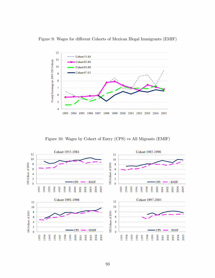
Figure 9: Wages for different Cohorts of Mexican Illegal Immigrants (EMIF)
Figure 10: Wages by Cohort of Entry (CPS) vs All Migrants (EMIF)
93

Figure 11: Wages by Cohort of Entry (CPS) vs Legal Permanent Migrants (EMIF)
Figure 12: Wages of Legal and Illegal Mexican Immigrants in the United States
94

5.2.1 Construction of Weights
A selection issue can arise if workers are more or less likely to cross depending on their
characteristics such as legal status or earnings, since they might appear in the sample at
different rates. In order to address this problem, using the number of times that each worker
has entered and exited the U.S., I estimate their probability of being observed in the sample
and construct a set of weights using the inverse of that probability.
Entries per yeari =Number of entriesi
Number of years in USi
for individual i observed in year t.
Probability of being observedi =Entries per yearit
i=n∑i=1
Entries per yearit
weightProb Entryi =1
Probability of being observedi
5.2.2 Matching Estimators and Propensity Score
Formally, let y1i be the outcome with treatment, y0i the outcome without treatment and x
denote a vector of observed covariates. Also let w be a binary treatment indicator, where
w = 1 denotes treatment (i.e. legal) and w = 0 otherwise (i.e. illegal). To measure the effect
of the treatment, we are interested in the difference in the outcomes y1− y0. However, since
y1 and y0 are not observed at the same time, the quantity of interest becomes the average
treatment effect on the treated (ATT) which is defined as:
ATT = τP,T = E[y1i − y0i|wi = 1]
The treatment effect can be identified non-parametrically by imposing two assumptions:
the conditional independence and the overlap assumptions. The first assumption states that
conditional on the covariates xi, wi and (y1i, y0i) are independent.
95

(y1i, y0i) ⊥ wi|xi
The second assumption states that for any value of x, there are some units that are
treated and other units that are not.
0 < P [wi = 1|xi] < 1
Given that eligibility to IRCA’s legalization program was exclusively based on date of
arrival to the U.S. (treatment group), we can presume that the conditional independence
assumption is satisfied. Additionally, one test that can be used to assess the validity of this
assumption is to compare the impact of treatment for different control groups. For that
reason, when I test for selectivity among workers obtaining legal status after entering the
U.S. illegally, and when I estimate the gain from legal status among workers legalized under
IRCA, results using two different control groups are analyzed (ineligible migrants, eligible
non-applicants and applicants for legal status under IRCA). With respect to the overlap
assumption, different tests to verify that the assumption is satisfied are also performed (e.g.
comparison of the distribution of the covariates for the treatment and control groups and
estimation under common support for the treatment and control groups).
5.2.2.1 Matching Estimator As was mentioned before, since only one of the potential
outcomes y1 or y0 is observed for each individual, matching estimators impute the missing
outcome for each i by finding other individuals whose covariates are similar, but who were
not exposed to the treatment. In other words, using average outcomes of individuals with
“similar”characteristics, we can estimate the wage that workers legalized under IRCA would
have earned if they had obtained legal status through other channels.
Under the conditional independence and overlap assumptions, the matching estimator
for the average treatment effect on the treated is
ATTMATCH =1
N
∑i|wi=1
µ1(xi)− µ0(xi)
96

Another characteristic of the matching method is that it allow us to estimate “exact
matching”using as matches observations of the opposite treatment status with the exact
same values of the regressors and also “inexact matching”if we use units that have “close”
covariate matches. An issue that arises with the inexact matching method is that we will
introduce a bias if we use as matches units that do not have exactly the same covariates, xi,
as unit i. In this paper I use a bias corrected matching estimator suggested by Abadie and
Imbens (2006) which calculates a counterfactual adjusted for the difference in the covariates
between a unit and its matches.
5.2.2.2 Propensity Score Rosenbaum and Rubin (1983) define the propensity score as
the conditional probability of treatment given the covariates
p(x) = Pr[w = 1|x].
The key result of Rosenbaum and Rubin is that if the balancing hypothesis1 is satisfied,
wi ⊥ xi|p(xi)
and if the conditional independence assumption is true
(y1i, y0i) ⊥ wi|xi
then treatment status, wi, is independent of the potential outcomes (y1i, y0i) conditional on
the propensity score p(x)
(y1i, y0i) ⊥ wi|p(xi).
Thus, rather than conditioning on the covariates, x, we can condition on the propensity
score, p(x), to estimate the treatment effects.
1The balancing hypothesis implies that observations with the same propensity score must have the samedistribution of observable (and unobservable) characteristics independently of treatment status. In otherwords, for a given propensity score, exposure to treatment is random and therefore treated and control unitsshould be on average observationally identical.
97

Today there exist numerous methods for using the propensity score; however, one of the
methods that has attracted most research interest in recent years is to use it in conjunction
with a matching method. One approach is to use nearest neighbor matching in which the
set of matches for unit i, JM(i), is defined as the M observations in the opposite treatment
group with the smallest values of the scalar distance
||p(x1)− p(xi)||.
Once this set of M nearest neighbors has been constructed, we can compute the ATT
using inexact matching based on the covariates xi. Another approach is to use radius match-
ing which is comparable to nearest neighbor matching but rather than define the M closest
neighbors, it only use matches that are within some predefined interval r such that
JM(i) = {i = 1, 2, .., N |W1 = 1−Wi , ||p(x1)− p(xi)|| < r}
While radius matching give equal weight to every match that lies within JM(i), there is
another method named kernel matching that determines the weight that each match receives
based on the distance of the match from the original unit.
Finally, another method for using the propensity score is known as stratification or
blocking. The idea is that, based on the propensity score, the data is divided into B blocks
so that the probability of treatment is approximately the same across observations in a
block. The estimate of the population ATT is determined by averaging the estimates within
each block and weighting by the share of the sample observations that fall in that block.
When using this method, I check whether the covariates are balanced, that is, whether the
difference between the average of the covariates for the treatment and control groups within
each block is small.
98
BIBLIOGRAPHY
[1] Abadie, A., Drukker, D., Herr, J. L. and Imbens, G. (2004). “Implementing matchingestimators for average treatment effects in Stata.”The Stata Journal (2004) 4, Number3, pp. 290—311.
[2] Abadie, A. and Imbens, G. (2006). “Large Sample Properties of Matching Estimatorsfor Average Treatment Effects." Econometrica, 74(1), 235-267.
[3] Albrecht, J., Navarro, L. and Vroman, S. (2009). “The Effects of Labour Market Policiesin an Economy with an Informal Sector,”Economic Journal, Royal Economic Society,vol. 119(539).
[4] Andolfatto, D. (1996). “Business Cycles and Labor-Market Search,”American EconomicReview, 86, 112-132.
[5] Angelucci, M. (2005). “U.S. Border Enforcement and the Net Flow of Mexican IllegalMigration,”IZA Discussion Papers 1642, Institute for the Study of Labor (IZA).
[6] Batalova, J. (2008). “Mexican Immigrants in the United States.”Migration Policy In-stitute.
[7] Bean, F. D., Corona, R., Tuiran, R., Woodrow-Lafield, K. A. and Van Hook, J. (2001). “Circular, Invisible, and Ambiguous Migrants.”Demography, Vol. 38 No.3, August2001, 411-422.
[8] Becker, S. and Ichino, A. (2002). ”Estimation of average treatment effects based onpropensity scores.”The Stata Journal, 2, Number 4, pp.358-377
[9] Beranek, W. (1982). “The Illegal Alien Work Force, Demand for Unskilled Labor, andthe Minimum Wage.”Journal of Labor Research, Vol. 3 (Winter): 89-99.
[10] Borjas, G. J. (1985). “Assimilation, Changes in Cohort Quality, and the Earnings ofImmigrants.”Journal of Labor Economics, Vol. 3, No. 4, pp. 463-489.
[11] Borjas, G. J. (1989). "Immigrant and Emigrant Earnings: A Longitudinal Study," Eco-nomic Inquiry 27 , 21-37.
99

[12] Borjas, G. J. (1994). “The economics of immigration”. Journal of Economic Literature,32, 1667—1717.
[13] Borjas, G. J. and Bratsberg B. (1996). “Who Leaves? The Outmigration of the Foreign-Born.”The Review of Economics and Statistics, Vol. 78, No. 1 (Feb., 1996), pp. 165-176.
[14] Borjas, G. J. (1999). “The Economic Analysis of Immigration." Handbook of LaborEconomics, Volume 3A, edited by Orley Ashenfelter and David Card, North-Holland,1999, pp. 1697-1760.
[15] Borjas, G. J. (2003). “The Labor Demand Curve is Downward Sloping: Reexaminingthe Impact of Immigration on the Labor Market,”Quarterly Journal of Economics, 118,no. 4:( 1335-1374.
[16] Borjas, G. J. and Friedberg, R. M. (2006). “The Immigrant Earnings Turnaround of the1990s.”Working Paper, Harvard University and Brown University.
[17] Borjas, G. J. and Lawrence, K. ( 2007). “The Evolution of the Mexican-Born Workforcein the United States” in Mexican Immigration to the United States. National Bureauof Economic Research Conference Report, Cambridge Ma.
[18] Bosh, M. (2007). “Job Creation and Job Destruction in the Presence of Informal LaborMarkets,”International Policy Center (IPC) - Working Paper Series No.52.
[19] Briggs, V. M. Jr. (2010), “Illegal Immigration and Immigration Reform: Protecting theEmployment Rights of the American Labor Force (Native-Born and Foreign-Born) WhoAre Eligible To Be Employed,”Center for Immigration Studies.
[20] Bunzel, H., Christensen, B., Kiefer, N., Korsholm, L., Muus, L.,Neumann, G., andRosholm, M. (2001) “Specification and Estimation of Equilibrium Search Models,”Re-view of Economics Dynamics, Volume 4, Issue 1, January, 90-126.
[21] Card, D. (2001), “Immigrant Inflows, Native Outflows, and the Labor Market Impactsof higher Immigration,”Journal of Labor Economics, 19(1): 22—64
[22] Card, D. (2005), “Is the New Immigration Really So Bad?,” Economic Journal,115(507): F300—23.
[23] Chiquiar, D. and Hanson, G. H. (2005). “International Migration, Self-Selection, andthe Distribution of Wages: Evidence from Mexico and the United States” Journal ofPolitical Economy 113(2): 239-281.
[24] Chiswick, B. R., (1978). “The Effect of Americanization on the Earnings of Foreign-bornMen.”The Journal of Political Economy, Vol. 86, No. 5, pp. 897-921.
[25] Chiswick, B. R., (1986). “Is the New Immigration Less Skilled Than the Old?”Journalof Labor Economics, Vol. 4, No. 2, pp. 168-192.
100

[26] Cobb-Clark, D. and Kossoudji, S. (2002). “Coming out of the Shadows: Learning aboutLegal Status and Wages from the Legalized Population.”Journal of Labor Economics,Vol. 20, No. 3.
[27] Congressional Budget Offi ce (2007). “The Impact of Unauthorized Immigrants on theBudgets of State and Local Governments.”Congress of the United States.
[28] Dehejia, R. (2005). “Practical propensity score matching: A Reply to Smith and Todd.”Journal of Econometrics 125, pp. 355—364.
[29] Den Haan, W. J., Ramey, G. and Watson, J. (2000). “Job Destruction and Propagationof Shocks,”American Economic Review, Vol. 90 (3), pages 482-498.
[30] Djajic, S. and Melbourne, R. (1988). “A General Equilibrium Model of Guest-workerMigration." Journal of International Economics 25:335-351.
[31] Duleep, H. O. (1994). “Social Security and the Emigration of Immigrants.”Social Se-curity Bulletin 57:37-52.
[32] Dustmann, C., (1995). “Savings behavior of migrant workers: A Life-Cycle Analysis.”Zeitschrift fFur Wirtschafts- und Sozialwissenschaften 115, 511—533.
[33] Dustmann, C., (1997). “Return Migration, Uncertainty and Precautionary Savings.”Journal of Development Economics, 52, 295—316.
[34] Dustmann, C. (2003). “Return Migration, Wage Differentials, and the Optimal Migra-tion Duration.”European Economic Review 47, 353—369.
[35] Friedberg, R. (2001), “The Impact of Mass Migration on the Israeli Labor Market,”Quarterly Journal of Economics 117(4), 1373—1408.
[36] Friedberg, R. and Hunt, J. (1995), “The Impact of Immigrants on Host Country Wages,Employment, and Growth,”Journal of Economic Perspectives 9(2), 23—44.
[37] Gertler, M., Trigari, A., (2009). “Unemployment fluctuations with staggered Nash wagebargaining. Journal of Political Economy 117, 38-86.
[38] Gitter, S., Gitter R. and Southgate, D. (2008). “The Impact of Return Migration toMexico,”Estudios Económicos, El Colegio de México, Centro de Estudios Económicos,Vol. 23(1), pp. 3-23.
[39] Gonzalez, H. (2011). “Selectivity in U.S. Immigration: Differences Between Legal andIllegal Mexican Immigrants”. Working Paper.
[40] Greenwood, M. J. and McDowell, J. M.(1999). “Legal U.S. Immigration: Influenceson Gender, Age, and Skill Composition.”Kalamazoo, MI: W.E. Upjohn Institute forEmployment Research.
101

[41] Hall, R. E. (1995). “Lost Jobs,”Brookings Papers on Economic Activity, (1), pp. 221—73.
[42] Hall, R. E.(2005). “Employment Effi ciency and Sticky Wages: Evidence from Flows inthe Labor Market,”National Bureau of Economic Research, Working Paper 11183.
[43] Hall, R. E. and Milgrom, P.R. (2008). “The Limited Influence of Unemployment onthe Wage Bargain,”American Economic Review, American Economic Association, vol.98(4), pages 1653-74, September.
[44] Hanson, G. H. and Spilimbergo, A. (1996). “Illegal Immigration, Border Enforcement,and Relative Wages: Evidence from Apprehension at the U.S.-Mexico Border.”NBERWorking Paper No. 5592, May 1996.
[45] Hanson, G. H., Robertson, R. and Spilimbergo, A. (2002). "Does Border EnforcementProtect U.S. Workers From Illegal Immigration?," The Review of Economics and Sta-tistics, MIT Press, Vol. 84(1), pp. 73-92, February.
[46] Hanson, G. H., (2006). “Illegal Migration from Mexico to the United States.”Journalof Economic Literature, December 44(2006): 869-924.
[47] Herzog, H., and Schottman, A. M. (1982). “Migration Information, Job Search and theRemigration Decision.”Southern Economic Journal, Vol. 50, No. 1, pp. 43—56.
[48] Hill, J. K. (1987). “Immigrant decisions concerning the duration of stay and migrationfrequency,”Journal of Development Economics, 25, 221—234.
[49] Hoefer, M., Rytina N., and Campbell C. (2008). “Estimates of the Unauthorized Immi-grant Population Residing in the United States: January 2007.”Department of Home-land Security.
[50] Hoefer, M., Rytina N., and Baker B. (2011). “Estimates of the Unauthorized ImmigrantPopulation Residing in the United States: January 2010.”Department of HomelandSecurity.
[51] Imbens G. and Wooldridge J. (2009) “New Developments in Econometrics.”Cemmap,UCL. June 2009, Lecture Notes 2.
[52] Jasso, G. and Rosenzweig, M. R. (1988). "How Well Do U.S. Immigrants Do? VintageEffects, Emigration Selectivity, and Occupational Mobility." Research in PopulationEconomics 6:229-253
[53] King, M., Ruggles, S., Alexander, T., Leicach, D. and Sobek, M. Integrated Public UseMicrodata Series, Current Population Survey: Version 2.0. Minneapolis, MN: MinnesotaPopulation Center, 2004.
[54] Krause, M., and Lubik, T., (2007). “The (Ir)relevance of Real Wage Rigidity in the NewKeynesian Model with Search Frictions,”Journal of Monetary Economics 54, 706-727.
102

[55] Kossoudji, S. and Cobb-Clark, D. (2002). “Coming out of the Shadows: Learning aboutLegal Status and Wages from the Legalized Population,”Journal of Labor Economics20, No.3, pp. 598-628.
[56] LaLonde, R. J. and Topel, R. H. (1991).”Immigrants in the American Labor Market:Quality, Assimilation, and Distributional Effects.” The American Economic Review,Vol. 81, No. 2, pp. 297-302.
[57] Lindstrom, D. P. (1996). “Economic Opportunity in Mexico and Return Migration fromthe United States”, Demography, Vol. 33, no. 3, 357-374.
[58] Massey, D. (1987). “Do Undocumented Migrants Earn Lower Wages than Legal Immi-grants? New Evidence from Mexico.”International Migration Review, Vol. XXI, No. 2,1987, pp. 236-274
[59] Massey, D. S., Arango, J., Graeme, H., Kouaoci A., Pellegrino A. and Taylor E. (1993),“Theories of International Migration: A Review and Appraisal.”Population and Devel-opment Review, Vol. 19, No. 4, pp. 699—751.
[60] McKenzie D., Gibson J., and Stillman S. (2006). “How Important is Selection? Experi-mental versus Non-Experimental Measures of the Income Gains from Migration.”WorldBank Policy Research Working Paper 3906, May 2006.
[61] Mesnard, A. (2004). “Temporary migration and capital market imperfections”OxfordEconomic Papers, 56, 242 —262.
[62] Millard, S., and Mortansen D. (1997): “The Unemployment and Welfare Effects ofLabour Market Policy,”in Unemployment Policy: Government Options for the LabourMarket, pp. 545—572. Cambridge.
[63] Mortensen, D. and Pissarides, C. (1994). “Job Creation and Job Destruction in theTheory of Unemployment,”Review of Economic Studies 61, 397-415.
[64] Mortensen, D. and Pissarides, C. (1999).“New developments in models of search in thelabor market,”in O. Ashenfelter and D. Card, eds., Handbook of Labor Economics Vol3: 2567-2627. Amsterdam: Elsevier Science, 1999.
[65] Orrenius, P. (2001). "Illegal Immigration and Enforcement along the Southwest Border."Border Economy 8, Federal Reserve Bank of Dallas, June 2001.
[66] Ottaviano, G. I. P. and Peri, G. (2010) “Rethinking the Effects of Immigration onWages,”Forthcoming in Journal of the European Economic Association, 2010.
[67] Passel, J. S. (2005). “Estimates of the Size and Characteristics of the UndocumentedPopulation,”The Pew Hispanic Center.
[68] Passel, J. S. (2006). “Size and Characteristics of the Unauthorized Migrant Population,”The Pew Hispanic Center.
103

[69] Passel, J. S., Capps, R. and Fix M. E. (2004). “Undocumented Immigrants: Facts andFigures,”Urban Institute Immigration Studies Program.
[70] Passel, J. S. and Cohn, D. (2009). “A Portrait of Unauthorized Immigrants in the UnitedStates,”The Pew Hispanic Center.
[71] Passel, J. S. and Cohn, D.(2010). “U.S. Unauthorized Immigration Flows Are DownSharply Since Mid-Decade,”The Pew Hispanic Center.
[72] Petrosky-Nadeau, N. (2009). “Credit, Vacancies and Unemployment Fluctuation,”GSIAWorking Paper #2009-E27, Carnegie Mellon University, Tepper School of Business.
[73] Pissarides, C. A. (1998). “The impact of employment tax cuts on unemployment andwages; The role of unemployment benefits and tax structure,”European Economic Re-view, Elsevier, Vol. 42(1), pp. 155-183, January.
[74] Pissarides, C. A. (2009). “The Unemployment Volatility Puzzle: Is Wage Stickiness theAnswer?,”Econometrica, Econometric Society, Vol. 77(5), pages 1339-1369, 09.
[75] Polgreen, L. and Simpson N. B. (2005). “Recent Trends in the Skill Composition ofLegal U.S. Immigrants.”Southern Economic Journal, Vol. 72, No. 4, pp. 938—957.
[76] Porter, E. (2005). "Illegal Immigrants Are Bolstering Social Security With Millions."New York Times, April 5, 2005.
[77] Reyes, B. and Mameesh, L. (2002). “Why Does Immigrant Trip Duration Vary AcrossU.S. Destinations?,”Social Science Quarterly, Vol. 83 (2), pp. 580-593.
[78] Rosenbaum, P. R. and Rubin, D. B. (1983). “The Central Role of the Propensity Scorein Observational Studies for Causal Effects.”Biometrika. 70:41-55.
[79] Rytina, N. (2001). “IRCA Legalization Effects: Lawful Permanent Residence and Nat-uralization through 2001.”Offi ce of Policy and Planning Statistics Division, U.S. Immi-gration and Naturalization Service.
[80] Sato, Y. (2004). “Migration, Frictional Unemployment, and Welfare-Improving LaborPolicies,”Journal of Regional Science, 44: 773—793.
[81] Shimer, R. (2005). “The Cyclical Behavior of Equilibrium Unemployment and Vacan-cies,”American Economic Review, Vol. 95 (1), pages 25-49.
[82] Sjaastad, L. (1962). "The Costs and Returns of Human Migration." The Journal ofPolitical Economy, Vol. 7 No.5, Part 2: Investment in Human Beings, pp. 80-93.
[83] Stark, O. (1991) The Migration of Labor. London: Basil Blackwell.
[84] Taylor, E. (1992). “Earnings and Mobility of Legal and Illegal Immigrant Workers inAgriculture.”American Journal of Agricultural Economics, Vol. 74, No. 4, pp. 889-896.
104

[85] U.S. Department of Homeland Security (2003). “Estimates of the Unauthorized Immi-grant Population Residing in the United States: 1990 to 2000.”
[86] U.S. Government Accountability Offi ce (2006). "GAO-06-770 Illegal Immigration:Border-Crossing Deaths Have Doubled Since 1995."
[87] Vernez, G. and Ronfeldt, D. (1991). “The Current Situation in Mexican Immigration,”Science 8, March 1991, Vol. 251. no. 4998, pp. 1189 —1193.
[88] Warren, R.(2003). “Estimates of the Unauthorized Immigrant Population Re-siding inthe United States: 1990-2000,” Offi ce of Immigration Statistics, U.S. Department ofHomeland Security.
[89] Wong, L. (2003). “Can the Mortensen-Pissarides Model with Productivity ChangesExplain U.S. Wage Inequality?,”Journal of Labor Economics, 1/2003.
105