AQUACULTURE ENVIRONMENT INTERACTIONSAquacult Environ Interact

Vol. 4: 81–90, 2013doi: 10.3354/aei00075

Published online June 26

INTRODUCTION

Aquaculture net cages for Pacific bluefin tunaThunnus orientalis are currently designed to with-stand rough conditions from ocean currents andwaves (Suzuki et al. 2009) but do not meet the biolog-ical requirements of this species. Because cultivatedtuna swim faster than other fishes, the shape, vol-ume, and dimensions of these cages need to be ade-quate to allow tuna to swim and turn, as it is likelythat the need to make sharp turns would stimulate

stress, reducing the quality of cultivated fish. There-fore, scientific information is required to determinethe most suitable cage radius to allow circling fish toturn along cage walls and to determine how tunaswim in all 3 dimensions within the cages, particu-larly since net cages are altered into various 3-dimensional (3D) shapes by the tidal current (Suzukiet al. 2009). Visualization of the 3D behavior of fishprovides data on their turning angle, the radius of theswimming circle, and the space used by individualswithin the cage. However, to complete such an

© The authors 2013. Open Access under Creative Commons byAttribution Licence. Use, distribution and reproduction are un -restricted. Authors and original publication must be credited.

Publisher: Inter-Research · www.int-res.com

*These authors contributed equally to this work**Corresponding author. Email: tutakagi@nara.kindai.ac.jp

Three-dimensional trajectories of cultivatedPacific bluefin tuna Thunnus orientalis in an

aquaculture net cage

Kazuyoshi Komeyama1,*, Minoru Kadota2,3,*, Shinsuke Torisawa2, Tsutomu Takagi2,**

1Faculty of Fishery, Kagoshima University, 4-50-20 Shimoarata, Kagoshima 890-0056, Japan2Department of Fisheries, Faculty of Agriculture, Kinki University, 3327-204 Naka-machi, Nara 631-8505, Japan

3Temple University, 4-1-27 Mita, Minato-ku, Tokyo 109-0073, Japan

ABSTRACT: Swimming trajectories of aquatic animals that are estimated using the dead- reckoning technique below the sea surface tend to have very large associated observationalerrors. Therefore, the aim of the present study was to develop a technique for removing accumu-lated errors from such trajectories for Pacific bluefin tuna Thunnus orientalis. Horizontal and ver-tical speeds and heading angle were measured in an aquaculture net cage using 2 types of dataloggers, and current velocity was recorded at a depth of 12 m to measure the tidal current speedaround the net cage. Fourier analysis indicated that the primary source of error in trajectory esti-mates was the effect of ocean currents, which resulted in drift, and further analysis revealed thatthe frequency contributing to drift was consistent with the low-frequency signal in a spectrumanalysis of horizontal speed. Therefore, a high-pass filter was applied to horizontal speed data toremove any frequencies lower than the cut-off frequency (0.0015 Hz), following which these datawere back-transformed into a time domain that no longer included the drift effect caused by thecurrent. The reconstructed trajectories fit within the inner diameters of the net cage, indicatingthat they were realistic. To confirm the validity of the resultant swimming trajectories, a flumetank experiment was conducted, which demonstrated that the high-pass filter effectively removedcurrent drift from the estimated trajectory. Furthermore, since the method was estimated to havea precision of approximately 0.20 m, it not only allows the 3-dimensional trajectories of circlingtuna to be estimated but can also be applied to the behavior of fish in the wild.

KEY WORDS: Dead reckoning · Behaviour · Submerged net cage

OPENPEN ACCESSCCESS

Aquacult Environ Interact 4: 81–90, 2013

analysis, new methods are needed to allow accuratemeasurement of the 3D trajectories of bluefin tuna.

A complete understanding of fish behavior belowthe sea surface remains elusive due to limitations ofthe available technology for making indirect under-water observations in both natural and enclosedareas. Although some studies have described the be -haviors of cultivated tuna in aquaculture net cages(Kubo et al. 2004, Okano et al. 2006, Kadota et al.2011), these have relied on measurements of 1Dswimming behavior, swimming depth, acceleration,and/or feeding behavior.

Two techniques are currently available for examin-ing the movements of aquatic animals below the seasurface: acoustic telemetry (e.g. Hindell et al. 2002)and dead reckoning (Wilson & Wilson 1988, Shiomi etal. 2008, Komeyama et al. 2011). Acoustic telemetryestimates the position of fish using acoustic transmit-ters that measure the difference in time the emittedsound takes to arrive at hydrophones (e.g. Harcourtet al. 2000, Hindell et al. 2002, Bégout Anras & La-gardère 2004). This method has several drawbacks,including that a receiver must be located within a fewhundred meters of the target fish, making it difficultto obtain data for species with extensive ranges (Wil-son et al. 2007); it is difficult to affix acoustic receiversin offshore areas; ocean waves and oscillations ofthe hydro phones by waves generate acoustic noise;changes in water temperature in the thermoclinestrongly affect the acoustic velocity; also, it is difficultto continuously detect the signal at a fine scale (i.e. afew seconds) to estimate high-resolution fish trajecto-ries. Thus, although acoustic telemetry has the ad-vantage of directly measuring the position of fish, itmay be difficult to measure fish behavior with a highaccuracy and over a fine time scale in offshore areas.

The dead-reckoning technique overcomes theseproblems by using a very simple principle. Specifi-cally, it requires data on a target’s speed, headingangle, and depth change per given interval; velocityvectors are then calculated and estimated indirectlybased on an observational dataset, following which3D trajectories can be constructed. Thus, dead reck-oning produces temporally resolved, regular, se -quen tial positional data with no gaps (Wilson et al.2002). However, this method also has drawbacks inthat the trajectories include cumulative error frommultiple sources. Some of this error is associated withthe lack of underwater reference points, but thegreatest source of inaccuracy originates from driftresulting from factors such as ocean currents andwinds (Bramanti et al. 1988, Mitani et al. 2003,Shiomi et al. 2008, Komeyama et al. 2011), and since

a trajectory is estimated by integrating velocity vec-tors, this inaccuracy increases with time.

Komeyama et al. (2011) measured the 3D trajecto-ries of bluefin tuna in a submerged aquaculture netcage and used linear detrending to remove accumu-lated error from the reconstructed trajectories. How-ever, the details of the trajectories were inadequate,and so only limited information could be estimatedbecause almost all of the reconstructed trajectoriesdrifted nonlinearly. In addition, there were no cleargrounds for detrending the linear component fromthe nonlinear drift, leaving room for improvement.

In the present study, we assessed the potentialsources of drift error due to ocean currents anddeveloped a new technique for removing this error toallow for a more accurate visualization of the trajec-tories of circling cultivated bluefin tuna in an aqua-culture net cage. To do this, we reanalyzed the be -havioral data described by Komeyama et al. (2011),to allow direct comparison with their results. Weattempted to reconstruct the 3D trajectories of tuna,which were calculated using a high-pass filter me -thod, and then confirmed the validity of the methodby conducting an experiment in a large flume tank.

MATERIALS AND METHODS

In the present study, we carefully analyzed thetime series of ocean current data that were collectedin an experimental net cage by Komeyama et al.(2011), using a high-pass filter to remove the drift sig-nal (which decreases slowly). To test the validity ofusing this high-pass filter method within the dead-reckoning technique, we confirmed the calculatedtrajectories using both a field and laboratory experi-ment.

Formulation of the dead-reckoning technique

The dead-reckoning technique was used to visual-ize the swimming paths of a single tuna in an aqua-culture net cage. Velocity vectors were estimatedbased on speed (v), heading angle (θ), and change indepth (d) per measurement interval (t) using the fol-lowing formulae:

(1)

(2)

(3)

v v vx t z tt t= − ⋅ θcos2 2

v v vx t z tt t= − ⋅ θsin2 2

v d dz t tt= − −1

82

Komeyama et al.: 3D trajectories of bluefin tuna 83

where Δt = 1 corresponds to the measurement inter-val, and the vector (vxt, vy, vzt) is a locomotion vectorat measurement time t. The 3D swimming pathcould then be reconstructed from the observationaldataset by integrating the locomotion vector withrespect to time (i.e. summing Eqs. 1 to 3) to give thefollowing:

(4)

(5)

(6)

However, the horizontal swimming paths obtainedusing Eqs. (4) and (5) include large cumulativeerrors (Shiomi et al. 2008, Komeyama et al. 2011),mostly due to the horizontal ocean current. By con-trast, the vertical swimming path given by Eq. (6)includes less cumulative error because the magni-tude of vertical currents is much lower than that ofthe horizontal current. Therefore, Eqs. (4) and (5)were decomposed into 3 terms (the tuna-locationterm, the current-drift term (cd), and the accumula-tion of error term) and then solved for tuna location.Thus, the tuna location at measurement time t canbe written as follows:

(7)

(8)

where xε,t and yε,t represent observational errors, andxu and yu represent errors associated with horizontalcurrent velocities (u). Thus, the net errors can beexpressed as follows:

(9)

(10)

To correct the estimated positional data, the neterrors of Eqs. (9) and (10) were then removed byassuming constant linear drift. However, positionsestimated in this way accumulate error with time andbecome more inaccurate simply because the oceancurrent is not at all constant. Therefore, we requiredalternative techniques that do not assume constantcurrent velocities to remove errors associated withocean currents.

Removing low-frequency drift

The summed observational data calculated usingEqs. (4) & (5) include low-frequency drift, likely as aresult of physical noise, the major cause of which isthe ocean current (corresponding to the second termsin Eqs. 7 & 8). If these biases due to physical noise arenot accounted for, they invalidate events related tothe biological signals of interest and substantiallydecrease the power of the statistical analysis. There-fore, the removal of low-frequency drift is one of themost important steps in reconstructing 3D fish trajec-tories. Unfortunately, this pre-processing step is alsoone of the most dangerous steps because the biologi-cal signal of interest may easily be removed if incor-rect filters are applied. To test the developed equa-tions and data treatment, in situ measurements wererequired.

Reconstructing swimming trajectories in a net cage

We conducted an experiment in a submerged netcage installed in offshore waters of Kochi Prefecture,Japan, to reanalyze the data of Komeyama et al.(2011). The diameter of the cage was 30 m, and thenet was completely submerged, with the ceiling lo -cated at a depth of 2 m and the floor at ~22 m belowthe surface.

A single bluefin tuna (fork length: 51 cm; estimatedweight: 2.6 kg taken from a regression line fit totuna-farm records) was captured from within thecage by angling. Two micro-data loggers (PD3GT,Little Leonardo, 75 g in air; DST Comp-Tilt, Star-Oddi, 19 g in air) that had been inserted into a singlefloating cellular material plate (9 cm long and 3.5 cmhigh), the buoyancy of which had been adjusted toslightly more than its underwater weight, were exter-nally attached to the body of the tuna near the seconddorsal fin (Komeyamaet al. 2011). The fish was thenreleased back into the net cage.

The PD3GT data logger recorded swimming speedand depth at 1 s intervals on a flash memory drivefrom 09:30 h on 6 March to 17:30 h on 7 March 2010.A propeller was attached to the PD3GT to record thespeed through the water, and we confirmed the rela-tionship between velocity and the number of pro-peller revolutions as well as the stall speed of thedevice (0.13 to 0.18 m s−1) in a preliminary experi-ment. In the study itself, the tagged fish swam atspeeds of >0.28 m s−1 without the propeller stopping.

The DST Comp-Tilt data logger recorded the head-ing of the fish, which was calculated using 2D geo-

x v vt t z tn

N

t∑= − ⋅ θ=

cos2 2

1

y v vt t z tn

N

t∑= − ⋅ θ=

sin2 2

1

z d dt t tn

N

∑= − −=

( )11

costuna,2 2

1, ,x v v x xt t z t

n

N

cd t tt∑= − ⋅ θ +=

ε

sintuna,2 2

1, ,y v v y yt t z t

n

N

cd t tt∑= − ⋅ θ + +=

ε

x xcd t un

N

∑==

,1

y ycd t un

N

∑==

,1

Aquacult Environ Interact 4: 81–90, 2013

magnetism at 1 s intervals. Due to the logger’s limitedmemory capacity, data from the DST Comp-Tilt weredivided into 4 phases of daily activity: dawn, 05:00−07:00 h; daytime, 11:30−12:30 h; dusk, 17:00−19:00 h;and night-time, 23:30−24:30 h. A summary of thedepths and turning angles of the tagged fish duringeach phase is presented in Table 1. Initially, wehypo thesized that rotation of the propeller on thePD3GT data logger would influence these measure-ments, as the rotation speed of the propeller wastransmitted through magnetic variation caused by amagnet attached to the propeller shaft. However, ourpreliminary experiment detected no significant influ-ence of this on compass measurements. The data log-gers were detached from the fish using a timingdevice and were collected by a diver after 3 d.

To monitor the current profile in the net cage, anelectromagnetic current meter (Infinity-EM; JFEAdvantec) was affixed to the outside of the net cageat a depth of 12 m from 14:30 h on 5 March until10:00 h on 12 March 2010. The meter recorded thecurrent speed and direction, which were calculatedfrom the 2D velocities at 5 min intervals. To estimatecurrent velocities, 30 samples were taken at 1 s inter-vals every 5 min.

To validate the swimming trajectories calculated inthe present study, we examined whether the trajecto-ries fit into the aquaculture net cage. We chose the

origin (0, 0, depth) as the starting point of a trajectory.Since the net cage had a bowl-like shape, with amaximum diameter of 30 m near the frame on top ofthe cage but a gradually decreasing dia meter within creasing depth due to the nets being pulled by thesinker, it was difficult to obtain data on the diameterof the cage at each depth. Therefore, we estimatedthis factor using Net geometry and Loading Analysis(NaLA) software (Takagi et al. 2002, Suzuki et al.2009), which numerically estimated the geometryand internal forces acting on the net and rigging.

Reconstructing trajectories in a flume tank

To test the validity of our technique, we also con-ducted experiments in a flume tank filled with fresh-water (Fig. 1). The channel dimensions of the ob -served area of the flume tank were 6.0 m length ×2.0 m width × 1.0 m depth, and the speeds of the car-riages were 0 and 0.1 m s−1. We set the PD3GT andDST Comp-Tilt data loggers at the tip of the rod thatlay vertically below the edge of a vinyl chloride disk(diameter: 1.8 m), which completed a lap over ~20 sat 0 m s−1 or 0.1 m s−1. After downloading measure-ment data from these data loggers, both trajectorieswere reconstructed.

RESULTS AND DISCUSSION

Reconstructing swimming trajectories ina net cage

Fourier analysis of the locomotion vector

We conducted a Fourier analysis of the loco-motion vector denoted in Eqs. (7) & (8) to deter-mine the strengths of the respective frequenciesof the swimming motion in the data. The powerspectra of the x-directional (horizontal) compo-nent of the locomotion vector xt was obtainedby integrating the velocities ob served over 1 hbetween 23:30 and 00:30 h (Fig. 2a). Two signif-icant peaks ap peared in the power spectrum,with the higher-frequency peak (0.0134 Hz)corresponding to a periodicity of 74 s, whichequaled the time needed for a tuna to swim 1circumference of the net cage. The second fre-quency peak (0.0008 Hz) was thought to be thedominant frequency contributing to drift, but itwas not clear which frequency should be usedas a cut-off to remove the drift error from the

84

Phase n Depth (m) Turning angle(h of day) (degree s−1) Q1 Q2 Q3 Q1 Q2 Q3

11:30−12:30 3600 16.36 18.99 20.55 6 13 2217:00−19:00 7200 17.82 19.04 19.97 6 12 2223:30−00:30 3600 13.91 15.43 16.65 5 12 2305:00−07:00 7200 12.60 14.35 16.60 7 16 35

Table 1. Number of sample, depth, and turning angle of a taggedtuna during each phase. Q1, Q2, and Q3 mean 25, 50, and 75%

quartiles, respectively

1 m Flow (0 or 0.1 m s–1) Data logger package

6 m

2 m

Dia. 1.8 m

Fig. 1. Schematic illustration of the flume tank experiment

Komeyama et al.: 3D trajectories of bluefin tuna

data. Therefore, we conducted a more thoroughana lysis of the ocean current.

Fourier analysis of the ocean current

We conducted a Fourier analysis on the time seriesof ocean current data to estimate which frequencycontributed to drift. The power spectra of the oceancurrent at a depth of 12 m within the net cage werecalculated over 6 d, including the day on which theexperiment was conducted (Fig. 2b). Although thedataset was not large, our analysis resolved the tidalsignatures, with significant peaks at ~24.4 h and

11.5 h and smaller significant peaksat 7.5 h. These spectral peaks wereconsistent with results reported byStockwell et al. (2004), who used datafrom >19 000 monthly time seriestaken from 262 data buoy sites andalso discovered peaks at 24, 12, and8 h along the frequency spectrum.Thus, our analysis suggested thatmost of the ocean current powerspectrum at a depth of 12 m was asso-ciated with the tidal signal, allowingus to remove the frequency that con-tributed a major portion of the drift bychoosing cut-off values of <8 h. Itshould also be noted that ocean cur-rents fluctuate over short periods, butthis high-frequency fluctuation wasignored as noise for the purpose ofreconstructing the 3D tuna trajecto-ries in the present study, as we wereonly concerned with a time scale of afew minutes to a few hours. Thus, wecalculated the energy that was con-centrated at a frequency greater than0.00021 Hz (the fourth peak inFig. 2a) and found that 31% of theocean current energy occurred atthese higher frequencies. This fluctu-ation in ocean current energy neededto be removed from our observationaldata; therefore, we reanalyzed thedata used by Komeyama et al. (2011)from a frequency perspective andconsidered the role of high frequen-cies to select an appropriate cut-offfrequency.

Reconstructed 3D trajectories and their validity

When reconstructing the 3D swimming paths ofbluefin tuna, Komeyama et al. (2011) assumed a con-stant linear drift over time and thus subtracted drifterror by means of the least-squares fit. However, ex -ternal effects such as ocean currents vary over time,invalidating the linear drift assumption and leading tolarge errors in the calculated swimming paths. There-fore, we compared the linear drift and high-pass filtermethods and evaluated the nonlinear components ofthe drift error from a frequency perspective.

Given the highly linear relationship between thex-component of the locomotion vector and time

85

2.5

2.0

1.5

1.0

0.5

00

0.00

20.

004

0.00

60.

008

0.01

00.

012

0.01

40.

016

0.01

80.

020

0.02

20.

024

0.02

60.

028

0.03

0

0.35

0.30

0.25

0.20

0.15

0.10

0.05

00 0.2 0.4 0.6 0.8 1.0

Frequency (×10–4 Hz)

Frequency (Hz)

a

b

1.2 1.4 1.6 1.8 2.0

Pow

erP

ower

(×10

4)

74 s

24.4 h

7.5 h

11.5 h

Fig. 2. (a) The power spectra of the x-directional component of the locomotionvector xt, which was obtained by integrating the observed velocities over 1 hbetween 23:30 and 00:30 h. Two significant peaks appear in the frequencyspectrum; the higher-frequency peak (0.0134 Hz) corresponds to a periodicityof 74 s, while the other frequency peak (0.0008 Hz) is thought to be the domi-nant frequency contributing to drift. (b) The power spectra of the ocean cur-rent at a depth of 12 m within the net cage. Significant peaks were observed at

around 24.4 h and 11.5 h, with smaller significant peaks at 7.5 h

Aquacult Environ Interact 4: 81–90, 2013

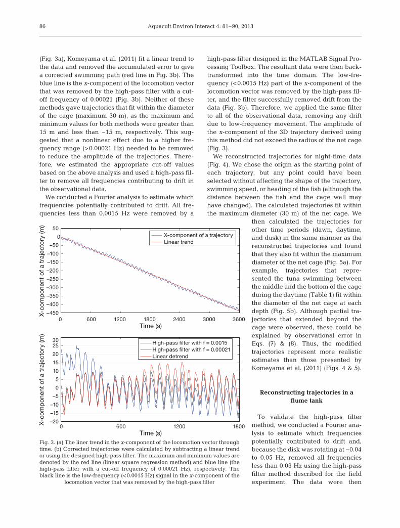
(Fig. 3a), Komeyama et al. (2011) fit a linear trend tothe data and removed the accumulated error to givea corrected swimming path (red line in Fig. 3b). Theblue line is the x-component of the locomotion vectorthat was removed by the high-pass filter with a cut-off frequency of 0.00021 (Fig. 3b). Neither of thesemethods gave trajectories that fit within the diameterof the cage (maximum 30 m), as the maximum andminimum values for both methods were greater than15 m and less than −15 m, respectively. This sug-gested that a nonlinear effect due to a higher fre-quency range (>0.00021 Hz) needed to be removedto reduce the amplitude of the trajectories. There-fore, we estimated the appropriate cut-off valuesbased on the above analysis and used a high-pass fil-ter to remove all frequencies contributing to drift inthe observational data.

We conducted a Fourier analysis to estimate whichfrequencies potentially contributed to drift. All fre-quencies less than 0.0015 Hz were removed by a

high-pass filter designed in the MATLAB Signal Pro-cessing Toolbox. The resultant data were then back-transformed into the time domain. The low-fre-quency (<0.0015 Hz) part of the x-component of thelocomotion vector was removed by the high-pass fil-ter, and the filter successfully removed drift from thedata (Fig. 3b). Therefore, we applied the same filterto all of the observational data, removing any driftdue to low-frequency movement. The amplitude ofthe x-component of the 3D trajectory derived usingthis method did not exceed the radius of the net cage(Fig. 3).

We reconstructed trajectories for night-time data(Fig. 4). We chose the origin as the starting point ofeach trajectory, but any point could have beenselected without affecting the shape of the trajectory,swimming speed, or heading of the fish (although thedistance between the fish and the cage wall mayhave changed). The calculated trajectories fit withinthe maximum diameter (30 m) of the net cage. We

then calculated the trajectories forother time periods (dawn, daytime,and dusk) in the same manner as thereconstructed trajectories and foundthat they also fit within the maximumdiameter of the net cage (Fig. 5a). Forexample, trajectories that repre-sented the tuna swimming betweenthe middle and the bottom of the cageduring the daytime (Table 1) fit withinthe diameter of the net cage at eachdepth (Fig. 5b). Although partial tra-jectories that extended beyond thecage were observed, these could beex plained by observational error inEqs. (7) & (8). Thus, the modified trajectories represent more realistic estimates than those presented byKomeyama et al. (2011) (Figs. 4 & 5).

Reconstructing trajectories in aflume tank

To validate the high-pass filtermethod, we conducted a Fourier ana -lysis to estimate which frequenciespotentially contributed to drift and,be cause the disk was rotating at ~0.04to 0.05 Hz, re moved all frequenciesless than 0.03 Hz using the high-passfilter method described for the fieldexperiment. The data were then

86

0 600 1200 1800 2400 3000 3600–450

–400

–350

–300

–250

–200

–150

–100

–50

0

50

Time (s)

X-co

mp

onen

t of

a t

raje

ctor

y (m

)

X-component of a trajectoryLinear trend

0 600 1200 1800–20

–15

–10

–5

0

5

10

15

20

2530

Time (s)

X-co

mp

onen

t of

a t

raje

ctor

y (m

)

High-pass filter with f = 0.0015High-pass filter with f = 0.00021Linear detrend

Fig. 3. (a) The liner trend in the x-component of the locomotion vector throughtime. (b) Corrected trajectories were calculated by subtracting a linear trendor using the designed high-pass filter. The maximum and minimum values aredenoted by the red line (linear square regression method) and blue line (thehigh-pass filter with a cut-off frequency of 0.00021 Hz), respectively. Theblack line is the low-frequency (<0.0015 Hz) signal in the x-component of the

locomotion vector that was removed by the high-pass filter

Komeyama et al.: 3D trajectories of bluefin tuna

back-transformed into the time domain. We removedthe steady flow along with the long-term trend usinga high-pass filter (Fig. 6). The filtered trajectorieswere not perfect circles but did approximate theshape of a circle. Therefore, we calculated the curva-ture radius of the estimated trajectories using 3points along each trajectory, which gave radii of 0.80± 0.17 m and 0.87 ± 0.16 m (mean ± SD) for the 0 m s−1

and 0.1 m s−1 conditions, respectively. The resultingSDs of 0.16 and 0.17 m suggested that the precisionof this method was ~0.20 m. The curvature radii ofthe 2 trajectories were similar to but lower than 0.90m, which is the radius of both true trajectories. Thisunderestimate may have been due to the response ofthe x- and y-components having been slightlydecreased during filtering. However, Hiraishi (2006)also reported that the propeller rotation sensitivity of

this device decreases drastically withincreasing angle of the incomingwater, which approaches a tilt of ~20°.In this flume tank experiment, theinclination angle of the propeller inrelation to the water flow directionchanged by 16° s−1 when the lap timewas 20 s; thus, the propeller rotationmay have been less sensitive to achange in the direction of movementdue to water flowing over it at thisinclined angle. This implies that if afish turns at a low curvature radius,the dead-reckoning technique using apropeller with attached data loggersmay underestimate the diameter ofthe trajectory. Turning angles greaterthan the 75% quartile had less of aneffect on trajectories in the flume tankex periment than in the field experi-ment (Table 1). However, althoughturning angles of >20° occurred a fewtimes in the field experiment, espe-cially during the period 05:00 to 07:00 h,the trajectories calculated in this ex -periment most likely represented thecorrect path. Thus, even though thepresent method may generate someunder estimations because the shapesof the filtered trajectories were bro-ken rather than circular (Fig. 6), this isun doubtedly the best currently avail-able method for estimating 3D trajec-tories.

CONCLUSIONS

Swimming speed measurements taken by thePD3GT data logger represent speed through thewater rather than relative to the ground, makingthem subject to tidal effects, and the drift trajectoryresults shown in Fig. 3 imply that the dead-reckoningtechnique cannot accurately estimate swimming tra-jectories where there are ocean/tidal currents. Shi -omi et al. (2008) applied a dead-reckoning techniquesimilar to the PD3GT used in the present study toreconstruct the 3D trajectories of emperor penguinsAptenodytes forsteri and suggested that the ac cumu -lated error was the result of ocean currents, andMitani et al. (2003) also recognized the influence ofcurrent flow when calculating trajectories. However,although these studies provided clear start and end

87

Fig. 4. Night-time (23:30 to 0:30 h) trajectories as reconstructed by the methods proposed in the present study. Colors of the trajectories indicate

swimming speeds

Aquacult Environ Interact 4: 81–90, 201388

–20

−10

010

20–2

0

–1001020

11:3

017

:00

23:3

005

:00

14–1

6m16

–18m

18–2

0m20

–22m

11:3

0

11:3

017

:00

23:3

005

:00

11:3

011

:30

11:3

0

Pre

sent

stu

dy

Pre

viou

s st

udy

(Kom

eyam

a et

al.

2011

)

Vert

ical

dis

trib

utio

n of

fish

tra

ject

orie

s in

pre

sent

stu

dy

m

m

–20

−10

010

20–2

0

–1001020

m

m

–20

−10

010

20–2

0

–1001020

m

m

–20

−10

010

20m

–20

−10

010

20m

–20

−10

010

20m

–20

−10

010

20m

–20

−10

010

20m

–20

−10

010

20m

–20

−10

010

20m

–20

−10

010

20m

–20

−10

010

20m

a b Fig

. 5. (

a) C

omp

aris

on o

f th

e tr

ajec

tori

es c

alcu

late

d f

or e

ach

tim

e p

erio

d in

th

e p

rese

nt

stu

dy

wit

h t

hos

e ca

lcu

late

d b

y K

omey

ama

et a

l. (

2011

). (

b)

Com

par

ison

of

the

di-

amet

er o

f th

e ca

ge

wit

h th

e d

iam

eter

of f

ish

cir

cles

at e

ach

dep

th a

s ca

lcu

late

d u

sin

g th

e m

eth

od d

evel

oped

in th

e p

rese

nt s

tud

y. T

hic

k b

lue

circ

ula

r li

ne

= th

e m

axim

um

d

iam

eter

of

the

sub

mer

ged

net

cag

e; t

hin

bla

ck li

nes

= t

he

calc

ula

ted

tra

ject

orie

s of

th

e tu

na

Komeyama et al.: 3D trajectories of bluefin tuna

points for the trajectories of animals, the recon-structed end points were not consistent with theactual end points.

In the present study, the fish was in the net cagethroughout the observational period. However, in theprevious study of Komeyama et al. (2011), the fish ap -peared to move outside the net cage, despite calmcurrent conditions, making it difficult to determinethe exact path taken by the fish because the locationwould have been influenced by tidal currents. Previ-ous studies have attempted to remove such effects byassuming a linear accumulation of errors; however,although this corrected a portion of the trajectoryerror, it did not completely remove temporal changesin the tidal component. Moreover, the current canchange in 3 dimensions, making it difficult to meas-ure current velocities. By contrast, the high-pass filter method used in the present study was effectiveat removing accumulated error even when therewere 3D changes in tidal flow, and the results of theflume tank experiment further indicated the useful-ness of this method for removing the tidal componentand accumulated error. However, the response of thefilter was extremely low near the start and end pointsdue to the filter’s characteristics. Further research isrequired to determine how to best overcome thisproblem (e.g. by excluding the first and last portions

of the trajectory from the analysis).However, the methods presented heregenerated sufficiently accurate trajec-tories to analyze the turning perform-ance and space use of the net cage bycultivated fish.

By analyzing the frequency of thecircling fish in combination with time-series data for current velocity, we de -termined the 3D trajectories of a blue -fin tuna circling within a submergedaquaculture net cage more ac curatelythan has been accomplished in previ-ous studies. The corrected paths helpto determine the swimming speed,inclination of the circle, and swim-ming depth at which fish swim (Fig. 4),providing useful information regard-ing the use of space by cultivated fishin aquaculture net cages. Given thatno monitoring techniques currentlyexist for cultivated tuna, we were notable to assess whether a causal rela-tionship exists between fish mortalityand reduced living space. However,we believe that visualization of the

trajectories of circling fish using the methods devel-oped in the present study will help increase the effi-ciency of bluefin tuna cultivation by contributing tofuture behavioral studies investigating how fish turnat cage walls (Bégout Anras & Lagardère 2004, Gau-trais et al. 2009) and the movement of fish schools inoutdoor cages.

The distance at which tagged fish swim from thewall of a net cage remains poorly understood, but wecould improve our knowledge of this factor by deter-mining the location of a fish within the cage or as -sess ing the distance of fish trajectories from the wall.To effectively use the method proposed in the pres-ent study to do this, several pass points of trajectoriesshould be measured to ensure they are correctlylocated and mimic the absolute coordinates.

Application of the proposed method may be lim-ited to circling fish in aquaculture, as additionalchallenges will be met when measuring trajectoriesof free-ranging aquatic animals in the open sea.However, exact trajectories in the open sea couldpotentially be estimated if one could remove anydrift components that fluctuate periodically, such astides. Alternatively, if noise sources cannot be iden-tified, acoustic telemetry could be used to detectfish positions within estimated trajectories in theopen sea.

89

Fig. 6. Results of the flume tank experiment. (a) Water stop, (b) steady flow(10 cm s–1). Black lines = reconstructed trajectories; blue lines = corrected trajectories from which accumulated error had been removed using the

high-pass filter method

Aquacult Environ Interact 4: 81–90, 2013

Acknowledgements. We express our sincere gratitude to Dr.Yuichi Tsuda (Fisheries Laboratory, Kinki University), Dr.Katsuya Suzuki (Nittoseimo Co.), Dr. Keigo Ebata, Mr. EitaOgata, Mr. Shoichi Nagano, Mr. Masataka Marugi (Facultyof Fisheries, Kagoshima University), the staff of Kinki Uni-versity for providing the specimens required for our study,and 3 anonymous referees for detailed suggestions onimproving this manuscript. We sincerely thank Mr. Kane -chiku (Kinki University) for his help and support with theNaLA System. We also thank Mr. S. Asaumi (Furuno Elec-tric), Mr. T. Kobayashi (Taiyo A&F), and the Association ofMarino-Forum 21 for their help and support. This work wassupported financially by a Grant-in-Aid for Young Scientists(B) (23780200) from the Ministry of Education, Culture,Sports, Science, and Technology and was supported in partby Grants-in-Aid for Scientific Research (C) (22580214) andfrom the Global COE program ‘Centre of Aquaculture Sci-ence and Technology for Bluefin Tuna and Other CultivatedFish’ of Kinki University from the Japan Society for the Pro-motion of Science.

LITERATURE CITED

Bégout Anras ML, Lagardère JP (2004) Measuring culturedfish swimming behaviour: first results on rainbow trout us-ing acoustic telemetry in tanks. Aquaculture 240: 175−186

Bramanti M, Dall’antonia L, Papi F (1988) A new techniqueto follow the flight paths of birds. J Exp Biol 134: 467−472

Gautrais J, Jost C, Soria M, Campo A and others (2009) Ana-lyzing fish movement as a persistent turning walker.J Math Biol 58: 429−445

Harcourt RG, Hindell MA, Bell DG, Waas JR (2000) Three-dimensional dive profiles of free-ranging Weddell seals.Polar Biol 23: 479−487

Hindell MA, Harcourt R, Waas JR, Thompson D (2002) Fine-scale three-dimensional spatial use by diving, lactatingfemale Weddell seals Leptonychotes weddellii. Mar EcolProg Ser 242: 275−284

Hiraishi T (2006) Dynamic analysis of cuttlefish basket trap.In: Yamamoto K, Yamane T, Mitsunaga Y (eds) Aquaticbiotelemetry and fishing gear telemetry. Kouseisyakou-seikaku, Tokyo, p 117−125

Kadota M, White EJ, Torisawa S, Komeyama K, Takagi T(2011) Employing relative entropy techniques for assess-

ing modifications in animal behavior. PLoS ONE 6: e28241

Komeyama K, Kadota M, Torisawa S, Suzuki K, Tsuda Y,Takagi T (2011) Measuring the swimming behaviour of areared Pacific bluefin tuna in a submerged aquaculturenet cage. Aquat Living Resour 24: 99−105

Kubo T, Sakamoto W, Kumai H (2004) Correlation betweenoceanic environmental fluctuation and bluefin tunabehavior in the aquaculture pen. Proc Int Symp SEA -STAR2000 and Bio-logging Science, December 13–15,2004, Bangkok, p 92−97

Mitani Y, Sato K, Ito S, Cameron MF, Siniff DB, Naito Y(2003) A method for reconstructing three-dimensionaldive profiles of marine mammals using geomagneticintensity data: results from two lactating Weddell seals.Polar Biol 26: 311−317

Okano S, Mitsunaga Y, Sakamoto W, Kumai H (2006) Studyon swimming behavior of cultured Pacific bluefin tunausing biotelemetry. Mem Fac Agric Kinki Univ 39: 79−82

Shiomi K, Sato K, Mitamura H, Arai N, Naito Y, Ponganis PJ(2008) Effect of ocean current on the 3-D dive paths ofEmperor penguins estimated by dead-reckoning. AquatBiol 3: 265−270

Stockwell RG, Lage WG, Milliff RF (2004) Resonant inertialoscillations in moored buoy ocean surface winds. TellusSer A Dyn Meterol Oceanogr 56: 536−547

Suzuki K, Torisawa S, Takagi T (2009) Numerical analysis ofnet cage dynamic behavior due to concurrent waves andcurrent. Proc ASME 2009 28th Int Conf Ocean, Offshoreand Arctic Engineering, May 31–June 5, 2009, Honolulu,HI, p 1−8

Takagi T, Suzuki K, Hiraishi T (2002) Development of thenumerical simulation method of dynamic fishing netshape. Bull Jpn Soc Sci Fish 68: 320−326

Wilson RP, Wilson, MP (1988) Dead reckoning — a new tech-nique for determining penguin movements at sea.Meeresforsch Rep Mar Res 32: 155−158

Wilson RP, Grémillet D, Syder J, Kierspel MAM and others(2002) Remote-sensing systems and seabirds: their use,abuse and potential for measuring marine environmentalvariables. Mar Ecol Prog Ser 228: 241−261

Wilson RP, Liebsch N, Davies IM, Quintana F and others(2007) All at sea with animal tracks; methodological andanalytical solutions for the resolution of movement.Deep-Sea Res II 54: 193−210

90

Editorial responsibility: Tim Dempster, Trondheim, Norway

Submitted: March 11, 2013; Accepted: May 24, 2013Proofs received from author(s): June 24, 2013