Three Centuries of Categorical Data Analysis:Log-linear Models and Maximum Likelihood

Estimation

Stephen E. Fienberg a,b Alessandro Rinaldo a

aDepartment of Statistics, Carnegie Mellon UniversitybCenter for Automated Learning and Discovery and Cylab, Carnegie Mellon

University

Abstract

The common view of the history of contingency tables is that it begins in 1900with the work of Pearson and Yule, but it extends back at least into the 19thcentury. Moreover it remains an active area of research today. In this paper wegive an overview of this history focussing on the development of log-linear modelsand their estimation via the method of maximum likelihood. S. N. Roy played acrucial role in this development with two papers co-authored with his studentsS. K. Mitra and Marvin Kastenbaum, at roughly the mid-point temporally in thisdevelopment. Then we describe a problem that eluded Roy and his students, that ofthe implications of sampling zeros for the existence of maximum likelihood estimatesfor log-linear models. Understanding the problem of non-existence is crucial to theanalysis of large sparse contingency tables. We introduce some relevant results fromthe application of algebraic geometry to the study of this statistical problem.

Key words: Algebraic statistics, Contingency tables, Chi-square tests, Log-linearmodels, Maximum likelihood, Multinomial sampling schemes, Sampling zeros

1 Introduction

Most papers and statistical textbooks on categorical data analysis trace thehistory back to the work of Karl Pearson and George Udny Yule at the turnof the last century. But as Stigler (2002) notes, there is an early history of

Email addresses: fienberg@stat.cmu.edu (Stephen E. Fienberg),arinaldo@stat.cmu.edu (Alessandro Rinaldo).

Preprint submitted to Elsevier Science 25 January 2006

contingency tables dating to at least the 19th century of Quetelet (1849) onmeasuring association and hypergeometric analysis for the 2 × 2 table byBienayme (see e.g., Heyde and Seneta, 1977), and the introduction by FrancisGalton (1892) of expected values of the form

Expected Count(i, j) =(Row Marginal Total i)× (Column Marginal Total j)

Grand Total,

(1)as a baseline for measuring association, a formula that would later play acrucial role in chi-square tests for independence. Categorical data analysisremains an active area of research today and thus our history covers activitiesthat span three centuries, the nineteenth, the twentieth, and the twenty-first,as is suggested by the title of this article.

The literature on categorical data analysis is now vast and there are manydifferent strands involving alternative models and methods. Our focus hereis largely on the development of log-linear models, maximum likelihood esti-mation, and the use of related chi-square tests of goodness of fit. In the nextsection of this paper we give an overview of the main part of this history be-ginning with the work of Pearson and Yule and running up to the present. S.N. Roy played a crucial role in this development with two papers co-authoredwith his students S. K. Mitra and Marvin Kastenbaum, at roughly the mid-point temporally in this development. We explain the importance of Roy’scontributions and how they influenced the development of the modern theoryof log-linear models. Then in Section 3, we turn our attention to a problemwhose full solution eluded statisticians beginning with the work of Bartlett(1935) until this past year, namely maximum likelihood estimation in thepresence of sampling zeros. In Section 4 and 5 we illustrate, largely throughexamples, the nature and implication of the sampling zeros problem and weintroduce the results that have begun to emerge from new tools in algebraicgeometry applied to statistics, an area recently dubbed as algebraic statistics

by Pistone et al. (2000).

2 Historical Development

As we mentioned at the outset, the history of categorical data analysis extendsback well into the 19th century. Here we pick up the history at the beginningof the 20th century, focusing largely on those contributions that frame thedevelopment of log-linear models and maximum likelihood estimation. We dothis in five parts: (1) Pearson-Yule through Neyman (1900-1950), (2) S. N.Roy’s contributions, (3) Emergence of log-linear models in the 1960s, (4) Themodern log-linear model era (1970s through present), (5) Other noteworthycategorical data models and methods. Agresti (2002) gives a complementary

2

historical overview.

2.1 Contingency Tables, Chi-Square, and Early Estimation Methods

The term contingency, used in connection with tables of cross-classified cat-egorical data, seems to have originated with Karl Pearson (1900) who, foran s × t table, defined contingency to be any measure of the total deviationfrom “independent probability.” The term is now used to refer to the tableof counts itself. Pearson (1900) laid the groundwork for his approach to con-tingency tables when he developed his chi-square test for comparing observedand expected (theoretical) frequencies:

X2 =�

i,j

(Observed Count(i, j)− Expected Count(i, j))2

Expected Count(i, j). (2)

Yet Pearson preferred to view contingency tables involving the cross-classificationof two or more polytomies as arising from a partition of a set of multivari-ate, normal data, with an underlying continuum for each polytomy. This viewled Pearson (1904) to develop his tetrachoric correlation coefficient for 2 × 2tables, and this work in turn spawned an extensive literature. The most seri-ous problems with Pearson’s approach were (a) the complicated infinite serieslinking the tetrachoric correlation coefficient with the frequencies in a 2 × 2table, and (b) his insistence that it always made sense to assume an underlyingcontinuum, even when the dichotomy of interest was dead–alive or employed–unemployed, and that it was reasonable to assume that the probability distri-bution over such a continuum was normal. In contradistinction, Yule (1900)chose to view the categories of a cross-classification as fixed, and he set out toconsider the structural relationship among the discrete variables representedby the cross-classification, via various functions of the cross-product ratios.Especially impressive in this, Yule’s first paper on the topic, is his notationalstructure for n attributes or 2n tables, and his attention to the concept ofpartial and joint association of dichotomous variables.

The debate between Pearson and Yule over whose approach was more appro-priate for contingency-table analysis raged for many years (see e.g., Pearsonand Heron, 1913), and the acrimony it engendered was exceeded only by thatassociated with Pearson’s dispute with R. A. Fisher over the adjustment inthe degrees of freedom (d.f.) for the chi-square test of independence associ-ated with a s × t table. In this latter case, Pearson, who argued that thereshould be no adjustment, was simply incorrect. As Fisher (1922) first noted,d.f. = (s − 1)(t − 1). In arguing for a correction or adjusted degrees of free-dom to account for the estimation of the parameters associated with the rowand column probabilities, Fisher built the basis for the asymptotic theory of

3

goodness of fit and model selection as we came to know it decades later. Inaddition, he related the estimation procedure explicitly with the characteriza-tion of structural association among categorical variables in terms of functionsof odds ratios proposed by Yule (1900) for the 2n table.

Bartlett (1935) introduced the first instance of a methodology for computingthe maximum likelihood estimates (MLEs) for contingency tables. The authorconsidered the case of what at the time would be called “complex contingencytables,” namely the 2 × 2 × 2 table displayed in Figure 1 for testing secondorder interactions. Bartlett showed that, in order to obtain the MLE under themodel with no-second-order interaction, one needs to solve a cubic equation todetermine a constant which then must be added and subtracted to the tablecells in an appropriate order. Norton (1945) extended Bartlett’s results to thecase of 2× 2× t tables.

Fig. 1. Bartlett’s representation of a 2× 2× 2 table (Bartlett, 1935, page 248).

Deming and Stephan (1940) proposed the method of iterative proportionalfitting (IPF) for estimating the cell values in a contingency table subject toconstraints coming from “known” marginal totals, e.g., from a populationdata set. The estimates were supposed to minimize a least squares criterionand were not related to statistical models of the sort usually associated withcontingency tables. The methodology became known as “raking” and foundwidespread application in sampling, especially at the U.S. Census Bureau andother national statistical offices.

Another noteworthy development from the 1930s was the likelihood ratio test,proposed by Wilks (1935) as an alternative to Pearson’s chi-square statistic:

G2 = 2�

i,j

Observed Count(i, j) log

�Observed Count(i, j)

Expected Count(i, j)

�

, (3)

with the same asymptotic distribution under the null hypothesis of indepen-dence of row and column variables. Neyman (1949) added to the array ofpossible chi-square tests, setting the stage for the work of Roy and his stu-dents.

4

2.2 S. N. Roy’s Contributions

S. N. Roy came to categorical data analysis from multivariate analysis morebroadly and his principal contributions were in collaboration with two Ph.D.students at the University of North Carolina during the mid-1950s, S. K. Mitraand Marvin Kastenbaum. These results were also described as a chapter inRoy (1957).

In the first of these papers, Roy and Mitra (1956) began by making a cleardistinction between response variables (‘variates’ in their terminology) andexplanatory variables (‘way of classification’), with the latter either being fixedby design or conditioned upon. They described the possible designs and modelsfor two-way and three-way contingency tables and discussed how these are tiedtogether through conditioning arguments, e.g. the model of homogeneity ofproportions in a two-way table consisting of one response and one explanatoryvariable has a likelihood function that is derivable through conditioning fromthe model of independence for a pair of response variables. Then they derivedasymptotic chi-square tests for these different situations, using the union-intersection principle Roy had developed in his earlier work on multivariateanalysis, and they showed that the “equivalent” hypotheses/designs have thesame maximum likelihood estimates and chi-square goodness-of-fit tests.

In the second paper, Roy and Kastenbaum (1956) filled in a major gap inthe framework of Roy and Mitra (1956). They derived a formal mechanismfor testing the hypothesis of no interaction in a 3-way table by offering new,“physically meaningful,” multiplicative functional representations of cell prob-abilities which they then used for computing the MLE via Lagrange multipli-ers. Like Bartlett and Norton before them, Roy and Kastenbaum did notconcern themselves with the possibility that some of the MLEs of the cellcounts could be negative. Nonetheless, they implicitly noted the role playedby “pivotal subscripts,” taking values 0, +1 and −1, which are used to addor subtract certain quantities to the observed cell counts, in order to computePearson’s chi-square statistic. As Birch (1963) would later point out, theseresults possess some undesirable properties, namely the estimates are not im-plicit functions of the frequencies and thus they are difficult to compute. Royand Kastenbaum (1956) concluded by suggesting how their models generalizefor higher-way tables.

Why did Roy and Kastenbaum not concern themselves with the existence ofthe MLE? While we can only speculate on the matter, the prevailing view atthe time was that one needed relatively large cell counts for the validity of theasymptotic distribution of the chi-square tests. For example, Cochran (1952,1954), in offering advice on the use of chi-quare tests, mentioned the need ofa minimum expected value of 1 and relatively few expectations less than 5. If

5

people were to follow this advice, then it is likely that they would encounterfew if any sampling zeros.

This advice was driven by Cochran’s attention to the comparison of the chi-square statistic with the exact distribution given the row and column totals,but the informal advice that resulted was that cell counts had to be at least5 to use the chi-square methodology (see the related discussion of Cochran’swork in Fienberg (1984). Thus for Roy and his students in the 1950s, samplingzeros did not pose an issue of statistical interest.

In the final section of his 1954 paper, Cochran presented a solution to themethod for combining tests across a series of n 2× 2 tables. This is in effect away to test for conditional independence of the two binary variables given nosecond-order interaction in the 2× 2×n table. The link was not noted in Royand Kastenbaums paper, and later Mantel and Haenszel (1959) independentlyproposed a similar test with two modifications.

Roy’s influence ran deeper than the two papers with Mitra and with Kasten-baum. One of his other Ph.D. students Vasant P. Bhapkar was to follow upon these ideas in a series of papers (e.g., see Bhapkar, 1961, 1966) and alsoin collaboration with Gary Koch (e.g., see Bhapkar and Koch, 1968). Thiswork led to the paper by Grizzle et al. (1969) and a number of subsequentcontributions by Koch and his students and colleagues.

2.3 The Emergence of Log-Linear Models and Methods

The 1960s saw a burgeoning literature on the analysis of contingency tables,largely but not solely focused on multiplicative or log-linear models. Key pa-pers by Birch (1963), Darroch (1962), Good (1963), and Goodman (1963,1964), plus the availability of high-speed computers, served to spur renewedinterest in the problems of categorical data analysis and especially log-linearmodels and maximum likelihood estimation. Fienberg (1992), in the introduc-tion to the reprinting of Birch (1963), details some of these developments.

Birch (1963) is, in many ways, the pivotal paper in the literature of the 1960sbecause it contains a succinct presentation of the basic results on maximumlikelihood estimation for n-way contingency tables for n ≥ 3, thereby general-izing and unifying the results derived by Roy and Mitra (1956) and Roy andKastenbaum (1956). First, Birch introduced the use of the logarithmic expan-sion of the cell mean vector in terms of u-factors, thus allowing for the generallog-linear representation and its connection with analysis of variance models.Then, under the assumption that the counts in the table are strictly positive,i.e., there are no sampling zero counts, he showed that the log-likelihood func-tion admits a unique maximum, identical for a variety of sampling schemes.

6

He also showed that the table marginal totals corresponding to the highest-order interaction terms in the model are the minimal sufficient statistics andthat these marginal totals are equal to the maximum likelihood estimates oftheir expectations. This last result provided a justification for using the itera-tive proportional fitting algorithm to compute the MLEs of the expected cellvalues, which is in fact based on a sequence of cyclic adjustments using themarginal totals.

Bishop (1967, 1969) used Birch’s results to derive connections between log-linear models and logit models, both from the theoretical and the computa-tional point of view. She also proposed using a version of the iterative propor-tional fitting method developed by Deming and Stephan (1940) to performcomputations for the MLE, as a practical way to implement the ideas of Birchto higher dimensional tables. The impetus for her work was the NationalHalothane Study, and Bishop applied the methodology to data from it. Be-cause the tables of interest from this study exceeded the capacity of the largestavailable computers of the day, she was led to explore ways to simplify theIPF calculations by multiplicative adjustments to the estimates for marginaltables—an idea related to models with direct multiplicative estimates such asconditional independence, studied by Roy and Mitra. Moreover, despite therelatively large sample sizes, by the time the data were spread across the cellsin the table, there were large numbers of zero counts, especially for the numer-ators in the rates of interest, i.e., surgical deaths in various categories. Thispractical application thus went well beyond the assumptions made by Birchand the literature that preceded him that the observed cell counts were allpositive. Yet the methodology worked well, suggesting that the assumptioncould clearly be relaxed.

Fienberg, whose research had also been motivated by applications in the Na-tional Halothane Study, gave in Fienberg (1970a) a geometrical proof of theconvergence of the IPF algorithm for tables with positive frequencies andshowed that the rate of convergence is linear. He drew on the geometric rep-resentation of contingency tables described in Fienberg (1968) and Fienbergand Gilbert (1970), papers that anticipated some of the recent representa-tions that have arisen in algebraic statistics. Then, in Fienberg (1970b), hegave sufficient conditions for the existence of unique non-zero maximum likeli-hood estimates for the expected cell counts in incomplete tables for the modelof quasi-independence, allowing for the presence of sampling zeros in the table.This allowed him to consider in an explicit manner the boundary points of thedomain of the log-likelihood function under the mean value parametrization.

Building on ideas in Bishop (1967, 1969), Goodman (1970, 1971) presentedmethods for analyzing n-way tables using log-linear models and likelihood ra-tio statistics. In particular, he considered the class of hierarchical log-linearmodels in which the cell mean vector is expressible in closed form as a ratio-

7

nal function of the sufficient statistics. For such models we can compute theMLE directly without resorting to any iterative numerical procedure. Good-man emphasized how these models are interpretable in terms of probabilityconcepts such as independence, conditional independence and equiprobability.Haberman (1974) referred to these as decomposable models and studied themmore thoroughly.

Generalizing the result by Birch to allow for sampling zeros, Haberman (1973)gave necessary and sufficient conditions for the existence of the MLE underPoisson and product-multinomial sampling schemes. One of his results pro-vides a clear justification for the Bartlett construction of the MLE via a se-ries of additions and subtractions of appropriate quantities to and from theobserved frequencies. This observation led naturally to the “pathological” ex-ample of a 2× 2× 2 table with positive margins and non-existent MLE shownin Figure 2. Haberman also gave an extended and rigorous proof, valid forgeneral multi-way tables and log-linear models, of Birch (1963)’s result thatthe marginal totals of the MLE of the cell mean vector match the observedmarginal totals and of the equivalence of the MLEs for Poisson and product-multinomial schemes. Furthermore, he provided a detailed study of IPF andNewton-Raphson’s method for computing the MLE, introduced the generalconditional Poisson sampling scheme for log-linear models, and gave an ex-tensive derivation of the asymptotic properties of the MLE. He included theseresults, along with many others, in his 1974 monograph, Haberman (1974).

n4

n2

n3

0

0n7

n6

n5

+!"!

"!+!

"!+!

+!"!

Fig. 2. 23 table with only two sampling zeros and the model of no-second-orderinteraction, using Bartlett’s notation from Figure 1. The two zero cells cause theMLE not to be defined because it is not possible to make one cell positive withoutmaking the other negative or changing the value of the margins.

Bishop et al. (1975) stressed the importance of being able to decide whetherthe MLE is defined or not and, more generally, to characterize the configu-rations of sampling zeros associated with a non-existent MLE. Further, theyraised concerns about the negative effect of a non-existent MLE on variousinferential procedures and, in particular, on model selection.

8

2.4 The Modern Log-linear Model Era: Graphical Models Through to Alge-

braic Geometry

Darroch et al. (1980) introduced the formalism and language of graph the-ory and Markov properties for modeling interactions in the context of log-linear models for contingency tables. By representing conditional independencethrough the absence of an edge in the graph, they initiated what is now the the-ory of graphical statistical models. They also provided a novel graph-theoreticderivation of the properties of decomposable models and their MLEs. Later,Gloneck et al. (1988) proved, by means of counter-examples, that positivity ofthe margins is a necessary and sufficient conditions for existence of the MLEif and only if the model is decomposable. This work ultimately led to threemajor books, by Whittaker (1990), Edwards (1995) and Lauritzen (1996),which demonstrated the usefulness of the graphical representation, both forinterpretation and for model search and related inferences, and which includedadditional theoretical insights.

Lauritzen (1996) offered many novel derivations of known results for decom-posable and other models using the powerful machinery of graphical models.Although he was not directly concerned with the problem of existence of theMLE, he defined the parameter space to be the sequential closure of the vectorsubspace describing the log-linear model, which he termed extended log-linear

models. By working with this enlarged parameter space, he was able to provethat the MLE is always defined, at least in an extended way, and furthermore,just as with the “ordinary” MLE, it satisfies the marginal equations.

Recent advances in the field of algebraic statistics, especially those followingDiaconis and Sturmfels (1998), have suggested a more general approach to thestudy of log-linear models that takes advantage of the connections betweenalgebraic and polyhedral geometry and the traditional theory of exponentialfamilies. Although Diaconis and Sturmfels (1998) originally introduced thisformalism for studying the “exact” distribution over contingency tables un-der a log-linear model given its minimal sufficient statistics, i.e. the observedmarginal totals , Fienberg (2000) suggested that these tools from algebraic ge-ometry would be of potential value beyond this problem. Eriksson et al. (2005)and Rinaldo (2005) have begun to deliver on that promise. We illustrate someof their findings in the next sections.

2.5 Some Other Notable Contributions to the Analysis of Categorical Data

There have been many other important contributions to the analysis of cat-egorical data over the past three decades which we do not have space to

9

document in the present paper. But we would be remiss if we did not at leastmention some of them even without extensive references:

• Model generation and testing using minimum modified chi-square estima-tion and the Wald statistic. This methodology emanated directly from thework of Roy and his students and often works for problems that do not havea convenient log-linear representation.

• Since the early 1970s much application involving log-linear models has beendone in the context of generalized linear models and GLM computing meth-ods. Unfortunately, as we explain in Section 4, these methods are not goodat handling the problems of zeros described in the next section.

• Goodman (1979, 1981) developed a special class of models which extendthe log-linear family by replacing various interaction terms by multiplica-tive counterparts. Such models, which are often referred to as “association”models are especially valuable when we are dealing with ordinal as opposedto nominal categorical variables and give reduced numbers of parameterscompared with traditional log-linear models.

• Correspondence analysis is yet another alternative to log-linear models thathas found adherents and its structure is close to but different from that of“association” models, which resemble log-linear models with multiplicativeinteraction terms.

• Rasch models for item response theory and latent class models have emergedas a powerful extension or alternative to traditional log-linear model anal-ysis.

• Bayesian methods for log-linear models have come into their own with theemergence of computation tools such as Monte Carlo Markov chain methods.

• A particular alternative to log-linear models that has emerged in the pasttwo decades is the Grade of Membership model (GOM) which can be inter-preted as a soft clustering methodology. The GoM turns out to be a specialcase of a class of Bayesian mixed membership models that work for textdata and images as well.

• Causal modeling uses the directed graphical structures that entered theliterature with Darroch et al. (1980). But the ideas from causal inferenceare more elaborate.

Goodman (1985, 1996) compares association and correspondence analysis mod-els. Erosheva et al. (2002) give a succinct comparison of log-linear, Rasch, andGoM models. Pearl (2000) and Spirtes et al. (2001) give treatments of causalmodeling including the role of latent variables and counterfactuals.

10

3 The Problem of Zeros and Existence of MLEs

Log-linear models are a powerful statistical tool for the analysis of categoricaldata and their use has increased greatly over the past two decades with thecompilation and distribution of large, and very often sparse, data bases, inthe social and medical sciences as well as in machine learning applications.In log-linear model analysis, the MLE of the expected value of the vector ofobserved counts plays a fundamental role for assessment of fit, model selectionand interpretation.

The existence of the MLE is essential for the usual derivation of large-samplechi-square approximations to numerous measures of goodness of fit (Bishopet al., 1975; Agresti, 2002; Cressie and Read, 1988) which are utilized toperform hypothesis tests and, most importantly, are an integral part of modelselection. If the distribution of the statistic measuring the goodness of fit isinstead derived from the “exact distribution,” or the conditional distributiongiven the minimal sufficient statistics (the margins), it is still necessary inmost cases to have an MLE or some similar type of estimate in order toquantify the discrepancy of the the observed data from the fitted values. Wealso require the existence of the MLE to obtain a limiting distribution in thedouble-asymptotic approximations for the likelihood ratio and Pearson chi-square statistic for tables in which both the sample size and the number ofcells are allowed to grow unbounded, a setting studied, in particular, by Morris(1975), Haberman (1977) and Koehler (1986) (see Cressie and Read, 1988, fora relatively complete literature review). If the MLE is not defined, inferentialprocedures such as those involved with model search that use chi-square toolsmay not be applied meaningfully or, at a minimum, require alteration.

As we noted in our historical review in the preceding section, the non-existenceof the MLE has long been known to relate to the presence of zero cell counts inthe observed table (see, in particular, Bishop, 1967; Goodman, 1970; Haber-man, 1974; Bishop et al., 1975). Indeed, a number of people informally ob-served that the only thing that appeared to matter was the numbers andlocations of the the sampling zeros and not the values of the counts in theremaining cells (see, e.g., Fienberg, 1970b). Although Haberman (1974) gavenecessary and sufficient conditions for the existence of the MLE, his char-acterization is nonconstructive in the sense that it does not directly lead toimplementable numerical procedures and also fails to suggest alternative meth-ods of inference for the case of an undefined MLE. Despite these deficiencies,Haberman (1974)’s results have remained all that exist in the published statis-tical literature. Furthermore, no one has presented yet a numerical procedurespecifically designed to check for existence of the MLE, and the only indicationof non-existence is lack of convergence of whatever algorithm is used to com-pute the MLE. As a result, the possibility of the non-existence of the MLE,

11

even though well known, is rarely a concern for practitioners. Moreover, evenfor those cases in which the non-existence is easily detectable, e.g. when theobserved table exhibits zero margins, there do not exist appropriate inferentialprocedures for dealing with such a situation.

Although zero counts can occur in small tables in which the expected valuesof some cells are significantly smaller than the others, they arise regularly inlarge tables in which the sample size is small relative to the number of cells.In particular, the non-existence of the MLE is potentially a very commonproblem in all applications in which the data are collected in the form oflarge and sparse databases, as in the social, biological and medical sciences.In many such cases, a common mispractice is to collapse the original table intosmaller, less sparse, tables with fewer categories or variables. As Bishop et al.(1975) and Asmussen and Edwards (1983) have made clear, such collapsingcan potentially lead to misleading and incorrect statistical inference aboutassociations among the variables.

Identifying the cases in which the MLE is not defined has immediate practi-cal implications and is crucial for applying appropriate modifications to tra-ditional procedures of model selection based on both asymptotic and exactapproximations of test statistics and for developing new inferential method-ologies to deal with sparse tables.

Eriksson et al. (2005) offered a novel geometric interpetation of the necessaryand sufficient conditions for the existence of the MLE as originally provedin Haberman (1974) for hierarchical log-linear models. Their findings werefurther generalized by Rinaldo (2005) to include non-hiearchial models andconditional Poisson sampling schemes. Overall, these results allowed for a fullcharacterization for all possible patterns of sampling zeros in the table causingthe MLE to be undefined and also led to efficient numerical procedures forchecking the existence of the MLE.

As initially noted by Haberman (1974) and later formalized by Lauritzen(1996), under mean value parametrization the log-likelihood function alwaysadmits a unique maximizer, even if the MLE is not defined; for cases in whichthe MLE does not exist, Haberman (1974) heuristically called these maximiz-ers extended MLEs. By combining results from the theory of linear exponentialfamilies (see, e.g., Brown, 1986) with results from algebraic geometry, Rinaldo(2005) provided a rigorous definition of extended MLEs, derived some of theirproperties and proposed a two-step procedure for performing extended max-imum likelihood estimation for log-linear models. In step one we identify theproblematic sampling zeros that cause the MLE not to exist, and then in step2 we condition on these and fit a a log-linear model to the remaining cells.

In the remainder of this article, we demonstrate, by means of examples, aspects

12

of the patterns of zeros that lead to non-existence of the MLE and variouspractical considerations that follow from the non-existence. We believe thatthe examples below give a good indication of the difficulties and subtleties,both computational and theoretical, associated with this problem.

Remark Throughout this article, we use the wording “non-existence of theMLE” to signify lack of solutions for the maximum likelihood optimizationproblem, in accordance with a terminology long established in the log-linearmodel literature (see, for example, Birch, 1963; Fienberg and Gilbert, 1970;Haberman, 1974). Alternatively, we can say that the MLE of the cell meanvector does not exist whenever there is no strictly positive solution to theMLE defining equations (see, for example, Haberman, 1974, Equation 2.11).

4 Illustrations of Non-Existence Problems

Since, as we mentioned, Haberman (1974)’s necessary and sufficient conditionsfor the existence of the MLE provide only a non-constructive characterization,it is not surprising that virtually all implemented computational algorithms forfitting log-linear models are, by design, incapable of handling these cases. Thefollowing excerpts from the SAS online documentation 1 for the PROC FREQ,PROC CATMOD and PROC GENMOD procedures exemplifies this situation.

• “By default, PROC FREQ does not process observations that have zero weights,

because these observations do not contribute to the total frequency count, and

because any resulting zero-weight row or column causes many of the tests

and measures of association to be undefined.”

• “For a log-linear model analysis using WLS or ML=NR, PROC CATMOD creates

response profiles only for the observed profiles. Thus, for any log-linear model

analysis with one population (the usual case), the contingency table will not

contain zeros, which means that all zero frequencies are treated as structural

zeros. If there is more than one population, then a zero in the body of the con-

tingency table is treated as a sampling zero (as long as some population has a

nonzero count for that profile). If you fit the log-linear model using ML=IPF,

the contingency table is incomplete and the zeros are treated like structural

zeros. If you want zero frequencies that PROC CATMOD would normally treat

as structural zeros to be interpreted as sampling zeros, you may specify the

ZERO=SAMPLING and MISSING=SAMPLING options in the MODEL statement.

Alternatively, you can specify ZERO=1E-20 and MISSING=1E-20.[...] sam-

pling zeros in the input data set should be specified with the ZERO= option

to ensure that these sampling zeros are not treated as structural zeros. Al-

ternatively, you can replace cell counts for sampling zeros by some positive

1 available at http://support.sas.com/onlinedoc/913/docMainpage.jsp

13

number close to zero (such as 1E-20) in a DATA step.”

• “PROC GENMOD treats each observation as if it appears n times, where n is

the value of the FREQ variable for the observation. If it is not an integer,

the frequency value is truncated to an integer. If it is less than 1 or if it is

missing, the observation is not used.”

In SAS, the presence of sampling zeros is dealt with by adding small positivequantities to the zero cells to facilitate the convergence of the underlyingnumerical procedure. This common practice can be very misleading, as theexample in Table 5 below demonstrates.

We illustrate various issues and dangers associated to the usage of very com-mon computational procedures for obtaining the MLE with artificially con-structed tables and with a simple real-life example of a non-sparse contingencytable. All the examples we present are still sufficiently small that, in principle,the user is able to detect lack of existence of the MLE by looking, heuristically,at the erratic behavior of the fitting algorithm or by applying directly someof the results from the theory. Both the theoretical results and the computa-tional tools available to researchers, however, are of little help when we go toanalyze high-dimensional complex and/or sparse databases.

4.1 Artificial Tables

Tables 1 and 2 show two examples of non-existent MLEs for the hierarchicallog-linear model of no-second-order interaction, [12][13][23]. In both cases, therelevant margins are strictly positive, a condition which in practice is veryfrequently, but erroneously, taken to be necessary and sufficient for the MLEto exist and in the literature has been described as “pathological” (Bishopet al., 1975, page 115).

We have already illustrated the cause of non-existence for Table 1 in Figure 2.For Table 2 we can conveniently explain non-existence by using collapsingarguments (see Eriksson et al., 2005, Section 4.1). If we collapse rows 1 and2 and columns 3 and 4, then the resulting pattern of zeros looks like thatin Table 1. But unlike the situation in Table 1, not all the zero cells impactnegatively on the existence of the MLE, i.e., the MLE would still not exist ifthe zero cell in position (1, 3) in the first array were to be replaced by anypositive count.

Despite the reduced dimension of both these tables, it is quite possible that,if we use standard statistical software for fitting log-linear models, we will notdetect non-existence. We illustrate the problem with a short computationalstudy of the behavior of two among the most commonly used algorithms to cal-culate the MLE: the IPF algorithm and the Iterative Weighted Least Squares

14

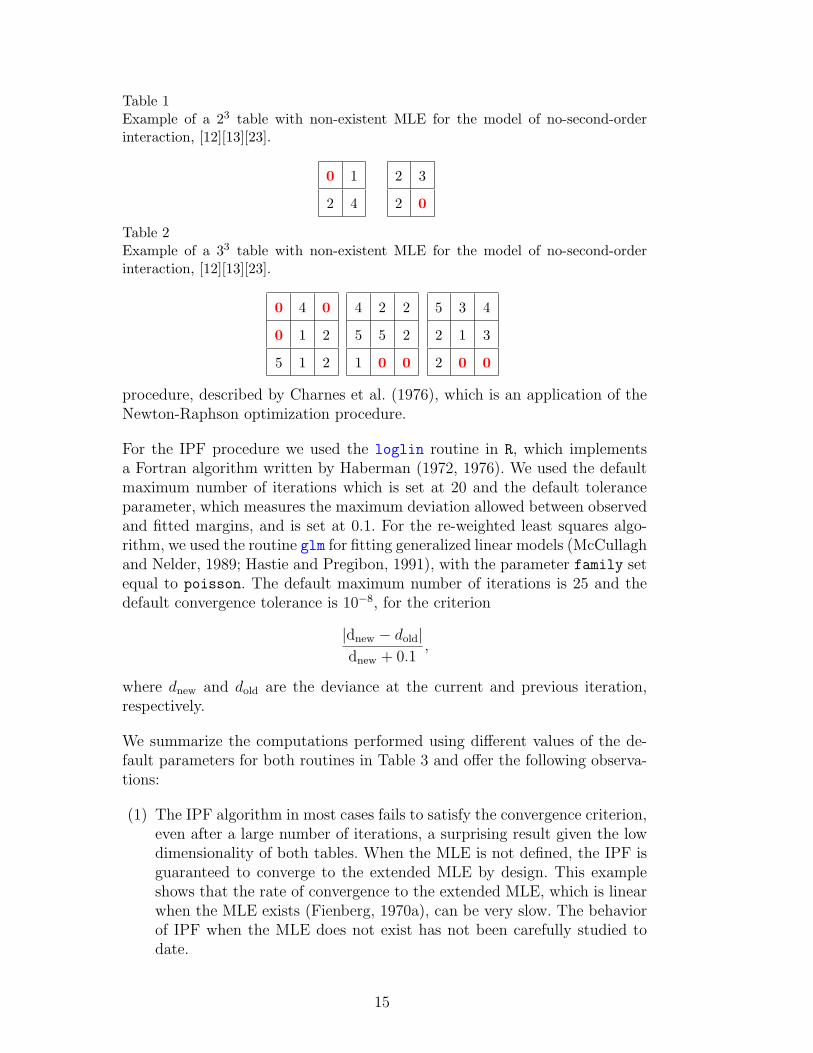
Table 1Example of a 23 table with non-existent MLE for the model of no-second-orderinteraction, [12][13][23].

0 1

2 4

2 3

2 0

Table 2Example of a 33 table with non-existent MLE for the model of no-second-orderinteraction, [12][13][23].

0 4 0

0 1 2

5 1 2

4 2 2

5 5 2

1 0 0

5 3 4

2 1 3

2 0 0

procedure, described by Charnes et al. (1976), which is an application of theNewton-Raphson optimization procedure.

For the IPF procedure we used the loglin routine in R, which implementsa Fortran algorithm written by Haberman (1972, 1976). We used the defaultmaximum number of iterations which is set at 20 and the default toleranceparameter, which measures the maximum deviation allowed between observedand fitted margins, and is set at 0.1. For the re-weighted least squares algo-rithm, we used the routine glm for fitting generalized linear models (McCullaghand Nelder, 1989; Hastie and Pregibon, 1991), with the parameter family setequal to poisson. The default maximum number of iterations is 25 and thedefault convergence tolerance is 10−8, for the criterion

|dnew − dold|dnew + 0.1

,

where dnew and dold are the deviance at the current and previous iteration,respectively.

We summarize the computations performed using different values of the de-fault parameters for both routines in Table 3 and offer the following observa-tions:

(1) The IPF algorithm in most cases fails to satisfy the convergence criterion,even after a large number of iterations, a surprising result given the lowdimensionality of both tables. When the MLE is not defined, the IPF isguaranteed to converge to the extended MLE by design. This exampleshows that the rate of convergence to the extended MLE, which is linearwhen the MLE exists (Fienberg, 1970a), can be very slow. The behaviorof IPF when the MLE does not exist has not been carefully studied todate.

15

(2) The Newton-Raphson procedure in the glm routine uses a more stringentconvergence criterion than the default ones for the loglin routine, be-cause it converges at a much faster rate than the IPF algorithm whena solution exists. Precisely because of its numerical robustness, however,the Newton-Raphson method does not provide any indication, at least insmall tables, that the MLE does not exists!

(3) When they fail to convergence, both procedures will simply produce awarning message along with the output of fitted values and the usualnumber of degrees of freedom, correct only for the case in which theMLE is defined.

These simple examples illustrate the fact that detecting non-existence of theMLE for tables with positive margins using available software requires a care-ful monitoring of the convergence of the algorithm used to calculate the MLE.Although the examples seem to suggest that the Newton-Raphson methodis computationally much more stable, in reality this is not the case. In fact,the estimated parameters of the glm routine tend to explode when the MLEdoes not exist because the maximum occurs on the boundary of the parame-ter space at minus infinity. Thus the numerical stability observed here is notimputable to the algorithm itself, but this is probably due to the small di-mensionality of these examples. Rinaldo (2005) proposed modifications of theNewton-Raphson procedure that allow it to exploit its fast rate of convergenceand, at the same time, to eliminate any exploding behavior.

4.2 Clinical Trial Example

Although non-existence of the MLE arises most frequently in sparse tables, itcan very well occur also in tables with large counts and very few zero cells.Table 4 shows a 2 × 2 × 2 × 3 contingency table from Koch et al. (1983),which describes the results of a clinical trial to examine the effectiveness ofan analgesic drug, for patients of two statuses and centers. The sample size isrelatively large (n = 193) with respect to the number of cells (p = 24) and,except for two zero counts, the cell counts are quite big.

With the goal of illustrating statistical disclosure limitation techniques anddiscussing the risk of disclosure associated to various marginal releases, Fien-berg and Slavkovic (2004) analyzed two nested models, both of which fit thedata of Table 4:

(1) [CST][CSR],(2) [CST][CSRT][TR].

The [CSR] margins has one zero entry, which causes the non-existence ofthe MLE for both models. Since the two models are decomposable (see, e.g.,

16

Table 3Summary of the computations performed on the Tables 1 and 2. Default valuesare marked with a (*).

Routine Tolerance Iterations Convergence Warnings

Table 1: 23 table and model [12][23][13]

loglin 1e-0 (*) 12 Yes

loglin 1e-05 20 (*) No stop("this should not happen")

loglin 1e-05 10,272 Yes

glm 1e-08 (*) 21 Yes

loglin 1e-08 500,000 No stop("this should not happen")

Table 2: 33 table and model [12][23][13]

loglin 1e-01 (*) 20 (*) No stop("this should not happen")

loglin 1e-01 27 Yes

loglin 1e-05 251,678 Yes

glm 1e-08 (*) 19 Yes

glm 1e-12 28 Yes

glm 1e-13 30 No fitted rates numerically 0

Lauritzen, 1996), the IPF algorithm converged almost instantaneously (lessthan 4 iterations) in both cases. In fact, the remarkable efficiency achievedby the IPF algorithm for decomposable models, demonstrated by Haberman(1974), is not affected by the non-existence (see Rinaldo, 2005). As a result,because of this fast rate of convergence, no indications of non-existence isprovided, except that some fitted values are zeros.

The pathology of zeros in the margins leading to non-existence is easy todetect and deal with as we have done here. The same type of pathology alsooccurs in the 2× 2× 2 and 3× 3× 3 tables.

4.3 Other Artificial Examples

The problem of non-existence of the MLE, even in 3-way tables, is not simplyreducible to collapsing or zeros in the margins, as is the case for the examplesof Table 2 and 4, respectively. However, more complex examples have beendifficult to construct until recently.

17

Table 4Results of clinical trial for the effectiveness of an analgesic drug. Source: Koch et al.(1983).

Response Poor Moderate Excellent

Center Status Treatment

Active 3 20 51

Placebo 11 14 8

Active 3 14 1212

Placebo 6 13 5

Active 12 12 01

Placebo 11 10 0

Active 9 3 422

Placebo 6 9 3

Table 5Example of a 33 table with non-existent MLE for the model of no-second-orderinteraction, [12][13][23].

0 2 0

5 1 4

0 2 3

2 2 3

1 0 4

0 0 2

3 5 0

1 0 0

2 4 1

Using a polyhedral geometry representation and the software package polymake(Gawrilow and Joswig, 2000), Eriksson et al. (2005) have been able to computethe number of degeneracies caused by patterns of zeros for p × q × r tablesfor p = 2, 3, and 4 and various choices of q and r, for the same no-second-order-interaction model. One of the first examples they discovered where thepattern of zeros is not simply characterized corresponds to the one illustratedin Table 5. After replacing the zero entries in this table with the small positivenumber 10−8, as recommended for the SAS procedures mentioned in Section4, we computed the MLE using the R routine loglin with a tolerance levelof 10−8 (incidentally, we note that the algorithm failed to converge within500, 000 iterations). The values of the X2 statistic (2) and of the G2 statistic(3) are 7.37021 × 10−6 and 1.472673 × 10−05, respectively, which, using a χ2

distribution with 8 d.f., results in p-values of nearly 1. In fact, the values ofboth goodness-of-fit statistics will always be almost zero, no matter what the

positive counts are. Thus for this pattern of zero cells, we virtually never rejectthe fitted model.

Eriksson et al. (2005) studied many other examples and observed that thenumber of possible patterns of zero counts invalidating the MLE exhibits an

18

Table 6Example of a 43 table with non-existent MLE for the model of no-second-orderinteraction, [12][13][23].

0 0 0 4

0 0 1 2

0 1 2 3

5 1 2 3

4 0 0 2

5 0 5 2

5 6 5 2

1 0 0 0

1 5 0 2

5 3 4 2

0 2 0 0

1 2 0 0

1 5 3 2

0 0 2 0

0 2 4 0

1 2 3 0

exploding behavior as the number of classifying variables or categories grows,so much so that computations become quickly unfeasible. Table 6 shows a morecomplex pattern for a larger 43 table. Note that, as was the case with Tables1, 2 and 5, the 2-way margins are strictly positive here, but we cannot reducethe problem to a lower dimensional non-esistence case through collapsing.

We leave it to the interested reader to test the computation of the MLE forthese tables in their favorite log-linear model computer program.

5 The 2K Table and The No-(K − 1)st-Order Interaction Model

In the 2× 2× 2 table with the no-second order interaction model all problemsof non-existence of the MLE come about if there are 2 zero counts. But notall pairs of zero counts cause problems. There are

�82

�= 28 ways to place 2

zeros in the table, and 12 of these pose no difficulties for maximum likelihoodestimation. These correspond to taking a row, a column, or a layer (6 possiblechoices) and placing zeros in the corners of the corresponding 2 × 2 table (2ways). The remaining 16 cases are degenerate. There can be a zero in a two-way marginal total and there are 12 possibilities for this to happen. And thenfinally we can place zeros into the “touching corners” of the full 23 table andthere are 4 ways to do this.

Now we consider the 2K contingency table and the model of no-(K−1)st-orderinteraction, for K ≥ 3. Suppose that the table contains only two samplingzeros and has positive margins. Because the model is very constrained, it isvery likely that the MLE does not exist. What we show is that the chance ofthis happening increases very fast with the number of factors K, a somewhatcounter-intuitive fact.

Proposition 1 For a 2K contingency table and the model of no-(K − 1)st-order interaction, the probability that two randomly-placed sampling zeros cause

19

the MLE not to exist without inducing zero margins is

(2K−1 −K)

(2K − 1). (4)

5 10 15 20 25

0.15

0.20

0.25

0.30

0.35

0.40

0.45

0.50

K

Fig. 3. Probability (4) that two randomly sampling placed zeros cause the MLEto be undefined without inducing zero margins as a function of the number K offactors for the 2K table and the model of no-(K − 1)st-order interaction, K ≥ 3.

PROOF. We prove this result using a counting argument by identifying eachpair of sampling zeros with one of the

�2K

2

�possible edges of the complete graph

on K vertices. The orthogonal complement in R2Kof the log-linear subspace

for the model of no-(K−1)st-order interaction has dimension 1 and is spannedby a 2K-dimensional vector δ, half of whose coordinates are +1 and the otherhalf are −1. By Theorem 2.2 in Haberman (1974), the MLE is not definedwhenever the two sampling zeros correspond to coordinates of δ of oppositesign. Therefore, the number of edges leading to an existing MLE is

2

�2K−1

2

�

= 2K−1(2K−1 − 1).

Since the number of edges associated to zero margins is K2K−1, the numberof edges causing the MLE not to be defined, without generating null margins,is

�2K

2

�− 2K−1(2K−1 − 1)−K2K−1 = 2K−1(2K − 1)− 2K−1(2K−1 − 1)−K2K−1

= 2K−1�2K − 1− 2K−1 + 1−K

�

= 2K−1(2K − 2K−1 −K)

= 2K−1(2K−1 −K).

20

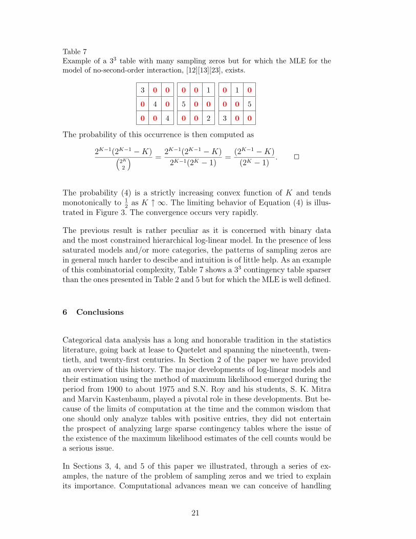
Table 7Example of a 33 table with many sampling zeros but for which the MLE for themodel of no-second-order interaction, [12][13][23], exists.

3 0 0

0 4 0

0 0 4

0 0 1

5 0 0

0 0 2

0 1 0

0 0 5

3 0 0

The probability of this occurrence is then computed as

2K−1(2K−1 −K)�

2K

2

� =2K−1(2K−1 −K)

2K−1(2K − 1)=

(2K−1 −K)

(2K − 1). ✷

The probability (4) is a strictly increasing convex function of K and tendsmonotonically to 1

2 as K ↑ ∞. The limiting behavior of Equation (4) is illus-trated in Figure 3. The convergence occurs very rapidly.

The previous result is rather peculiar as it is concerned with binary dataand the most constrained hierarchical log-linear model. In the presence of lesssaturated models and/or more categories, the patterns of sampling zeros arein general much harder to descibe and intuition is of little help. As an exampleof this combinatorial complexity, Table 7 shows a 33 contingency table sparserthan the ones presented in Table 2 and 5 but for which the MLE is well defined.

6 Conclusions

Categorical data analysis has a long and honorable tradition in the statisticsliterature, going back at lease to Quetelet and spanning the nineteenth, twen-tieth, and twenty-first centuries. In Section 2 of the paper we have providedan overview of this history. The major developments of log-linear models andtheir estimation using the method of maximum likelihood emerged during theperiod from 1900 to about 1975 and S.N. Roy and his students, S. K. Mitraand Marvin Kastenbaum, played a pivotal role in these developments. But be-cause of the limits of computation at the time and the common wisdom thatone should only analyze tables with positive entries, they did not entertainthe prospect of analyzing large sparse contingency tables where the issue ofthe existence of the maximum likelihood estimates of the cell counts would bea serious issue.

In Sections 3, 4, and 5 of this paper we illustrated, through a series of ex-amples, the nature of the problem of sampling zeros and we tried to explainits importance. Computational advances mean we can conceive of handling

21

larger and larger tables in our statistical analyses, and this inevitably meanswe must face up to the problem of the existence of the MLE. Until the recentintroduction of ideas from algebraic geometry into statistics, we had few toolsto do so in a constructive fashion. The examples we have used to illustrateexistence characterizations are drawn from Eriksson et al. (2005) and Rinaldo(2005). We hope to implement the characterizations in these sources in actualcomputer programs in the near future.

Silvapulle (1981) gave necessary and sufficient conditions for the existence ofthe MLE in binomial response models. These conditions are formulated interms of convex cones spanned by column vectors of the design matrix andappear to be closely related to the polyhedral conditions for the existence ofthe MLE in log-linear models derived by Eriksson et al. (2005). The studyof the connections between the non-existence of the MLE for log-linear mod-els and for logistic models involving categorical covariates deserves thoroughinvestigation.

We conclude by discussing some issues relating the problem of non-existenceof the MLE with conditional, or “exact”, inference. Being caused by the pres-ence of sampling zeros, non-existence of the MLE is more likely to occur insparse tables with small counts, a setting in which the traditional χ2 asymp-totic approximation to various measures of goodness of fit is known to beunreliable (see, e.g., Cressie and Read, 1988). In these cases, inference can beconducted by using as a reference distribution the conditional distribution ofthe tables given the observed sufficient statistics (i.e. the margins), also knownas the “exact” distribution. Starting with the seminal work of Diaconis andSturmfels (1998), new results from algebraic statistics have provided powerfulcharacterizations of the exact distribution and have emphasized the consider-able difficulties associated with sampling from it. For example, recent work byDe Loera and Onn (2005) demonstrated that the exact distribution can in factbe largely disconnected and possibly multi-modal and that the computationalcomplexity of any sampling procedure cannot be bounded. With respect tothe problem of the existence of the MLE, we note that the computation of theconditional distribution of measures of goodness of fit is closely related withthe existence of the MLE. In fact, when the MLE does not exist, all the tablesin the support of the exact distribution have zero entries precisely in the cellsfor which the expected counts cannot be estimated using maximum likelihood.Moreover, for log-linear models there are no general results characterizing theoptimality of exact methodologies. For exponential families, conditioning onthe sufficient statistics is a device for eliminating nuisance parameters andfor obtaining optimal tests and confidence intervals; however, the validity ofthis approach has been shown only for restricted models and very small ta-bles (see, e.g., Agresti, 1992; Lehmann and Romano, 2005) and it is unclearwhether it can be extended to general log-linear models on tables of arbitrarydimension. Further, it is unclear whether the exact distribution provides tools

22

for inference in sparse tables that can be considered optimal in some sense.

ACKNOWLEDGMENTS

The research reported here was supported in part by NSF grants EIA9876619and IIS0131884 to the National Institute of Statistical Sciences and draw inpart on material from earlier historical overviews by the first author, includ-ing the one in Fienberg (1980), as well as from the Ph.D. dissertation of thesecond author. We thank a referee for helpful comments and the reference toSilvapulle (1981).

References

Agresti, A., 1992. A survey of exact inference for contegency tables. StatiticalScience 7, 131–153.

Agresti, A., 2002. Categorical Data Analysis, 2nd Edition. Wiley, New York.Asmussen, S., Edwards, D., 1983. Collapsibility and response variables in con-

tingency tables. Biometrika 70, 567–578.Bartlett, M. S., 1935. Contingency table interactions. Supplement to the Jour-

nal of the Royal Statistical Society 2 (2), 248–252.Bhapkar, V. P., 1961. Some tests for categorical data. Annals of Mathematical

Statistics 29, 302–306.Bhapkar, V. P., 1966. A note on the equivalence of two test criteria for hy-

potheses in categorical data. Journal of the American Statistical Association61, 228–235.

Bhapkar, V. P., Koch, G. G., 1968. On the hypotheses of ”no interaction” incontingency tables. Biometrics 24, 567–594.

Birch, M. W., 1963. Maximum likelihood in three-way contingency tables.Journal of the Royal Statistical Society 25, 220–233.

Bishop, Y. M. M., 1967. Multi-dimensional contingency tables: Cell estimates.Ph.D. thesis, Department of Statistics, Harvard University.

Bishop, Y. M. M., 1969. Full contingency tables, logits, and split contingencytables. Biometrics 25 (2), 119–128.

Bishop, Y. M. M., Fienberg, S. E., Holland, P. W., 1975. Discrete MultivariateAnalysis. MIT Press, Cambridge, MA.

Brown, L. D., 1986. Fundamental of Statistical Exponential Families. Vol. 9 ofIMS Lecture Notes-Monograph Series. Institute of Mathematical Statistics,Hayward, CA.

Charnes, A., Frome, E. L., Yu, P. L., 1976. The equivalence of generalized

23

least squares and maximum likelihood estimates in the exponential family.Journal of the American Statistical Association 71 (353), 169–171.

Cochran, W. G., 1952. The χ2 test of goodness of fit. Annals of MathematicalStatistics 23, 315–345.

Cochran, W. G., 1954. Some methods for strengthening the common χ2 tests.Biometrics 10, 417–451.

Cressie, N. A. C., Read, T. R. C., 1988. Goodness-of-Fit Statistics for DiscreteMultivariate Data. Springer-Verlag, New York.

Darroch, J. N., 1962. Interaction in multi-factor contingency tables. Journalof the Royal Statistical Society 24, 251–263.

Darroch, J. N., Lauritzen, S. L., Speed, T. P., 1980. Markov fields and log-linear interaction models for contingency tables. Annals of Statistics 8 (3),522–539.

De Loera, J., Onn, S., 2005. Markov bases of three-way tables are arbitrarilycomplicated. Journal of Symbolic Computation, in press.

Deming, W. E., Stephan, F. F., 1940. On a least square adjustment of asampled ffrequency table when the expected marginal totals are known.Annals of Mathematical Statistics 11, 427–444.

Diaconis, P., Sturmfels, B., 1998. Algebraic algorithms for sampling from con-ditional distributions. Annals of Statistics 26 (1), 363–397.

Edwards, D., 1995. Introduction to Graphical Modelling. Springer-Verlag, NewYork.

Eriksson, N., Fienberg, S. E., Rinaldo, A., Sullivant, S., 2005. Polyhedral con-ditions for the nonexistence of the mle for hierarchical log-linear models.Journal of Symbolic Computation, in press.

Erosheva, E. A., Fienberg, S. E., Junker, B. W., 2002. Alternative statisticalmodels and representations for large sparse multi-dimensional contingencytables. Annales de la Faculte des Sciences de Toulouse 11 (4), 485–505.

Fienberg, S. E., 1968. The geometry of an r × c contingency table. Annals ofMathematical Statistics 39 (4), 1186–1190.

Fienberg, S. E., 1970a. An iterative procedure for estimation in contingencytables. Annals of Mathematical Statistics 41, 907–917.

Fienberg, S. E., 1970b. Quasi-independence and maximum likelihood estima-tion in incomplete contingency tables. Journal of the American StatisticalAssociation 65 (232), 1610–1616.

Fienberg, S. E., 1980. The Analysis of Cross-Classified Categorical Data, 2ndEdition. MIT Press, Cambridge, MA.

Fienberg, S. E., 1984. The contributions of William Cochran to categoricaldata analysis. In: Rao, P. S. R. S. (Ed.), W. G. Cochran’s Impact on Statis-tics. Wiley, New York, pp. 103–118.

Fienberg, S. E., 1992. Introduction to paper by M. W. Birch. In: Kotz, S.,Johnson, N. (Eds.), Breakthroughs in Statistics: Volume II, Methodologyand Distribution. Springer-Verlag, New York, pp. 453–461.

Fienberg, S. E., 2000. Contingency tables and log-linear models: Basic resultsand new developments. Journal of the American Statistical Association 95,

24

643–647.Fienberg, S. E., Gilbert, J. P., 1970. The geometry of a two by two contingency

table. Journal of the American Statistical Association 65 (330), 694–701.Fienberg, S. E., Slavkovic, A. B., 2004. Making the release of confidential data

from multi-way tables count. Chance 17 (3), 5–10.Fisher, R. A., 1922. On the interpretation of χ2 from contingency tables, and

the calculation of p. Journal of the Royal Statistical Society 85 (1), 87–94.Galton, F., 1892. Finger Prints. Macmillan, London.Gawrilow, E., Joswig, M., 2000. Polymake: a framework for analyzing con-

vex polytopes. In: Polytopes, Combinatorics and Computation. Birkhauser,Boston, MA.

Gloneck, G., Darroch, J. N., Speed, T. P., 1988. On the existence of the max-imum likelihood estimator for hierarchical log-linear models. ScandinavianJournal of Statistics 15, 187–193.

Good, I. J., 1963. Maximum entropy for hypotheses formulation especially formultidimensional contingency tables. Annals of Mathematical Statistics 34,911–934.

Goodman, L. A., 1963. On methods for comparing contingency tables. Journalof the Royal Statistical Society 126, 94–108.

Goodman, L. A., 1964. Simultaneous confidence limits for cross-product ratiosin contingency tables. Journal of the Royal Statistical Society 26, 86–102.

Goodman, L. A., 1970. The multivariate analysis of qualitative data: Inter-actions among multiple classifications. Journal of the American StatisticalAssociation 65 (329), 226–256.

Goodman, L. A., 1971. Partitioning of chi-square, analysis of marginal con-tingency tables, and estimation of expected frequencies in multidimensionalcontingency tables. Journal of the American Statistical Association 66 (334),339–344.

Goodman, L. A., 1979. Simple models for the analysis of association in cross-classifications having ordered categories. Journal of the American StatisticalAssociation 74, 537–552.

Goodman, L. A., 1981. Association models and canonical correlation in theanalysis of cross-classifications having ordered categories. Journal of theAmerican Statistical Association 76, 320–334.

Goodman, L. A., 1985. The analysis of cross-classified data having orderedand/or unordered categories: Association models, correlation models, andasymmetry models for contingency tables with or without missing entries.The Annals of Statistics 13, 10–69.

Goodman, L. A., 1996. A single general method for the analysis of cross-classified data: Reconciliation and synthesis of some methods of Pearson,Yule, and Fisher, and also some methods of correspondence analysis andassociation analysis. Journal of the American Statistical Association 91,408–428.

Grizzle, J. E., Starmer, C. F., Koch, G. G., 1969. Analysis of categorical databy linear models. Biometrics 24, 489–504.

25

Haberman, 1974. The Analysis of Frequency Data. University of ChicagoPress, Chicago, IL.

Haberman, S. J., 1972. Log-linear fit for contingency tables - Algorithm AS51.Applied Statistics 21, 218–225.

Haberman, S. J., 1973. Log-linear models for frequency data: Sufficient statis-tics and likelihood equations. Annals of Statistics 1 (4), 617–632.

Haberman, S. J., 1976. Correction to as 51: Log-linear fit for contingencytables. Applied Statistics 25 (2), 193.

Haberman, S. J., 1977. Log-linear models and frequency tables with smallexpected counts. Annals of Statistics 5 (6), 1148–1169.

Hastie, T. J., Pregibon, D., 1991. Generalized linear models. In: Cham-bers, J. M., Hastie, T. J. (Eds.), Statistical Models in S. Wadsworth &Brooks/Cole, Pacific Grove, CA.

Heyde, C. C., Seneta, E., 1977. I. J. Bienayme : Statistical Theory Anticipated.Springer-Verlag, New York.

Koch, G., Amara, J., Atkinson, S., Stanish, W., 1983. Overview of categoricalanalysis methods. SAS–SUGI 8, 785–795.

Koehler, K. J., 1986. Goodness-of-fit tests for log-linear models in sparse con-tingency tables. Journal of the Americal Statistical Association 81 (394),483–493.

Lauritzen, S. F., 1996. Graphical Models. Oxford University Press, New York.Lehmann, E. L., Romano, J. P., 2005. Testing Statistical Hypothesis, 3rd

Edition. Springer-Verlag.Mantel, N., Haenszel, W., 1959. Statistical aspects of the analysis of data from

retrospective studies of disease. Journal of the National Cancer Institute 22,719–748.

McCullagh, P., Nelder, J. A., 1989. Generalized Linear Models. Chapman andHall, New York.

Morris, C., 1975. Central limit theorems for multinomial sums. Annals ofStatistics 3 (1), 165–188.

Neyman, J., 1949. Contributions to the theory of the χ2 test. In: Proceed-ings of the Berkeley Symposium on Mathematical Statistics. University ofCalifornia Press, Berkeley, pp. 239–273.

Norton, H, W., 1945. Calculation of chi-square for complex contingency tables.Journal of the American Statistical Association 40 (230), 251–258.

Pearl, J., 2000. Causality: Models, Reasoning, and Inference. Cambridge Uni-versity Press, New York.

Pearson, K., 1900. On the criterion that a given system of deviation from theprobable in the case of a correlated system of variables is such that it canreasonably be supposed to have arisen from random sampling. PhilosophicalMagazine 50, 59–73.

Pearson, K., 1904. Mathematical contributions to the theory of evolution, XIII:On the theory of contingency and its relation to association and normalcorrelation. Draper’s Co. Research Memoirs in Biometry Ser. I, 1–35.

Pearson, K., Heron, D., 1913. On theories of association. Biometrika 9, 159–

26

315.Pistone, G., Riccomagno, E., Wynn, W. P., 2000. Algebraic Statistics: Com-

putational Commutative Algebra in Statistics. Chapman & Hall/CRC, NewYork.

Quetelet, M., 1849. Letters Addressed to H. R. H. the Grand Duke of SaxeCoburg and Gotha on the Theory of Probabilities as Applied to the Moraland Political Sciences (translated from the French by Olinthus GregoryDowns). Charles and Edwin Layton, London.

Rinaldo, A., 2005. Maximum likelihood estimates in large sparse contingencytables. Ph.D. thesis, Department of Statistics, Carnegie Mellon University.

Roy, S. N., 1957. Some Aspects of Multivariate Analysis. Wiley, New York.Roy, S. N., Kastenbaum, M. A., 1956. On the hypothesis of no “interaction”

in a multi-way contingency table. Annals of Mathematical Statistics 27 (3),749–757.

Roy, S. N., Mitra, S. K., 1956. An introduction to some nonparametric gener-alizations of analysis of variance and multivariate analysis. Biometrika 43,361–376.

Silvapulle, M. J., 1981. On the existence of maximum likelihood estimatorsfor the binomial response models. Journal of the Royal Statistical Society43 (3), 310–313.

Spirtes, P., Glymour, C., Scheines, R., 2001. Causation, Prediction, andSearch, 2nd Edition. MIT Press, Cambridge, MA.

Stigler, S., 2002. The missing early history of contingency tables. Annales dela Faculte des Sciences de Toulouse 11 (4), 563–573.

Whittaker, J., 1990. Graphical Models in Applied Multivariate Statistics. Wi-ley, New York.

Wilks, S. S., 1935. The liklihood test of independence in contingency tables.Annals of Mathematical Statistics 6, 190–196.

Yule, G. U., 1900. On the association of attributes in statistics: with illustra-tion from the material of the childhood society, &c. Philosophical Transac-tion of the Royal Society 194, 257–319.

27