Three approaches to the assessment of spatio-temporal distribution … · los del escurrimiento se...

Investigaciones Geográficas, Boletín del Instituto de Geografía, UNAMISSN 0188-4611, Núm. 76, 2011, pp. 34-55

Three approaches to the assessment of spatio-temporaldistribution of the water balance: the case of the Cuitzeo basin, Michoacán, Mexico Received: 20 September 2010. Final version accepted: 23 March 2011

Alfredo Amador García *Erna Granados López**Manuel E. Mendoza***

Abstract. Spatial distribution of the energy and flows of the hydrologic cycle in the form of evapotranspiration, runoff and infiltration within a region is a function of the climate (precipitation, temperature and evaporation) and landscape (relief, soil, land cover) of the area, and constitutes the hydrological cycle. The general model evaluating each of these sections and flows is the water balance. Methods for calculating the water balance in a region are based on either mass transference or energy transference. The aim of the present work was to calculate the spatially distributed regional water balance in a poorly gauged basin by each of three methods, and to evaluate these methods by comparing the results. Spatial modelling of the hydrometeorological variables used the ArcView 3.2 geographic information system; hydrological modelling made using HEC system version 3.1.0. The first approach was based on analysis of the information recorded at the available meteorological stations, point estimation of the monthly water balance according to the Thornthwaite and Mather method, and the

use of Thiessen polygons. The second approach was based on the calculation and distribution of the parameters for the Thornthwaite and Mather method. The third approach used the FAO–Penman equation. The models were applied to the Lake Cuitzeo basin. The result obtained by the third method indicated a mean annual volume of runoff of 229.05 hm3.This volume is only 8.5 hm3 less than that estimated as ne-cessary for maintaining a depth of 1 m throughout the Lake Cuitzeo water body. This difference represents a possible fluctuation of 2 cm in the mean level of the surface of the lake. The HEC model represents an alternative for modelling the basin since it requires relatively few inputs, of which the main ones (temperature, precipitation, potential evapotrans-piration, evapotranspiration) are obtainable or deducible by means of one or other of the approaches presented here.

Key words: Spatial modelling, water balance, poorly gauged basins, watershed management.

* Facultad de Biología, Universidad Michoacana de San Nicolás de Hidalgo, Ciudad Universitaria, Edif. R, 58030, Morelia, Michoacán, Mexico. E-mail: [email protected]* Departamento de Geología y Mineralogía, Instituto de Investigaciones Metalúrgicas, Universidad Michoacana de San Nicolás de Hidalgo, Ciudad Universitaria, Edif. U, 58030, Morelia, Michoacán, México. E-mail: [email protected]*** Centro de Investigaciones en Geografía Ambiental (CIGA), Universidad Nacional Autónoma de México, Antigua Carretera a Pátzcuaro No. 8701, Col. Ex Hacienda de San José de la Huerta, 58190, Morelia, Michoacán, Mexico. E-mail: [email protected]

Investigaciones Geográficas, Boletín 76, 2011 ][ 35

Three approaches to the assessment of spatio-temporal distribution of the water balance: the case of the Cuitzeo basin...

INTRODUCTION

The spatial distribution of the energy and the flows of the hydrologic cycle in the form of vapour (evapotranspiration), runoff and infiltration in a region are a function of its climate (precipitation, temperature and evaporation) and landscape (relief, soil and land cover) (He et al., 2000; Mendoza et al., 2002). Measurement, estimation and mode-lling of changes in the values of these flows can reveal critical areas of a basin and can influence decisions appropriate for water management. One of the key components of the water balance is evapotranspiration. This is a concept coined in 1948 by C.W. Thornthwaite, who was the first to devise a method for the regional estimation of this parameter (Hewlett, 1982). According to Ward and Trimble (2003), evapotranspiration is so important that it can represent a magnitude and proportion equivalent to the quantity of water that occurs in the form of runoff or infiltration at the global level and in the balance of many basins.

In general, it is considered that evapotrans-piration under more or less natural conditions

shows less annual variation than parameters such as precipitation or runoff. However, thinning of vegetation and change in land use can significantly reduce this parameter, so that consideration of the water balance has revealed consequent increases of up to 70% in the annual runoff (Hewlett, 1982).

The combination of methods for determining evapotranspiration (ET) and the execution of a spatially distributed hydrologic model based on evaluation of morphometric, climatic and bio-physics characteristics of the study area represents an opportunity to model the runoff (Q). In its turn, this allows evaluation of the optimal scenarios for ET, and hence is a useful method in supporting decision-making in water management for the basin. This is because it can group spatio-temporal units of hydrologic response (SCS, 1972; Hay et al., 1993; Neitsch et al., 2001) that can be incorporated into simulations of runoff and periods of retention of moisture in the basin, either under present con-ditions or in projections of possible trends or best-case projections of land-use change in the basin.

With regard to the Cuitzeo basin in Michoacán, Mexico, some studies have focused on a review of

Tres aproximaciones para estimación y distribuciónespacio-temporal del balance hídrico: el caso de la cuencade Cuitzeo, Michoacán, MéxicoResumen. La distribución espacial de la energía y los flujos de ciclo hidrológico en forma de vapor (evapotranspiración), escurrimiento e infiltración en una región, son una función de las características climáticas (precipitación, temperatura y evaporación) y del paisaje (relieve, suelo y cobertura) de un área y constituyen el llamado ciclo hidrológico. El modelo general de evaluación de cada uno de los compartimentos y flujos es el balance hídrico. Los métodos desarrollados para calcular el balance hídrico de una región toman como base el enfoque de transferencia de masa o el de transferencia de energía. Este trabajo se planteó como objetivo calcular, comparar y evaluar tres aproximaciones en la estimación del balance hídrico regional espacialmente distribuido en cuencas sin datos de aforos. El modelamiento espacial de las variables hidrometeorológicas se efectuó en el sistema de in-formación geográfica ArcView 3.2, y el modelamiento de los del escurrimiento se realizó con el sistema HEC versión 3.1.0. La primera aproximación está basada en el análisis de la información registrada en las estaciones meteoroló-gicas disponibles, estimación puntual del balance hídrico mensual conforme al método de Thornthwaite y Mather y

de polígonos de Thiessen; la segunda, en el cálculo y distri-bución de los parámetros para la aplicación del Método de Thornthwaite y Mather; finalmente la tercera aproximación se basó en el uso de la ecuación de FAO – Penman. Se escogió a la cuenca del lago de Cuitzeo como área de aplicación de los modelos. Destaca que mediante el resultado de la 3ª aproxi-mación el volumen anual promedio de escurrimientos co-rresponde a 229.05 hm3. Dicho volumen es apenas 8.5 hm3

inferior al estimado como necesario para mantener 1 m de profundidad en la extensión del cuerpo de agua del lago de Cuitzeo. Esta diferencia representa en esa misma extensión una eventual fluctuación de 3 cm en el nivel medio del espejo del lago. El modelo HEC representa una alternativa para el modelamiento de la cuenca ya que demanda relativamente de pocos insumos, los principales (T, PP, PET, ET) obtenibles o espacializables mediante alguna de las aproximaciones presentadas aquí.

Palabras clave: Modelamiento espacial, balance hídrico, cuencas sin aforo, manejo de recursos hídricos.

36 ][ Investigaciones Geográficas, Boletín 76, 2011

Alfredo Amador García, Erna Granados López and Manuel E. Mendoza

environmental characteristics of the water body and the sources of its contamination (Alvarado et al., 1994), while another branch of study has focused on description and analysis of the land cover and its changes (López et al., 2001 and 2006).

Studies specific to the hydrology of this basin include those by Mendoza et al. (2010) and Carlón et al. (2009). The former records the water balance across the study area and involves application of the Thornthwaite and Mather (1957) method, checking the precipitation and runoff in the types of cover prevailing in contrasting periods (the years 1975 and 2000). The results are assigned to ranks or classes (very low, low, moderate, high and very high) that group the separate annual estimations of the components of the water balance such as soil moisture deficit (SMD), soil moisture surplus (SMS), and actual evapotranspiration (AET).

Carlón et al. (2009), based on geographic infor-mation as well as the application of cluster analysis and principle components analysis; it proposes a subdivision of 59 sub-basins that it then groups into ten assemblages of relative similarity.

The evaluation of the water supply in basins with little or no gauging is important at both national and international levels (Osman, 1996; Elkaduwa and Sakthivadivel, 1998; Mendoza et al., 2002; Fuentes et al., 2004; Ziegler et al., 2005; Mendoza et al., 2010). The aim of the present study was to calculate and compare three approaches to the estimation of the water balance at the regional level and spatially distributed in poorly gauged basins. This objective involves the following:

• to estimate and assign potential evapotrans-piration (PET), AET and Q according to the Thornthwaite and Mather (1957) method;

• to estimate and assign Evapotransporation of Reference (ET0), Evapotranspiraction from crops or land cover (ETc) and Q according to the FAO-Penman (1990) method;

• to subdivide the basin in hydrological terms; and

• to estimate Q according to the US Soil Conserva-tion Service guidelines, supplementing and im-plementing the HEC model with the two previous approximate estimates, in a reference sub-basin.

STUDY AREA

The closed basin of Lake Cuitzeo is a hydrologic unit belonging to the Lerma region and lying in the Transverse Volcanic System, at 19°30’–20°05’ N and 100°35’–101°30’ W (Figure 1). Of its 3873.82 km2 area, the greater part lies in Michoacán State, and a small part in Guanajuato State. Mean annual precipitation in the basin is calculated as 847 mm and the annual mean temperature ranges between 16° and 18°C over most of the area (Mendoza et al., 2006), with the exception of the high country where temperatures are 14-16°C. On the basis of the criteria established by García (2004), three climatic types were recognized for the stations for this study: semi-warm, temperate and semi-arid. Mendoza et al. (2006) describe the existence of six geomorphological landscapes (sensu Zinck, 1988): plains, piedmonts, hills, low hills and mountains. There are in the basin eleven principal units of soil according to the FAO (1990) classificatory system: the greater part of the basin is covered by Vertisols, Luvisols and Acrisols, characterized as soils with predominantly fine textures (Mendoza et al., 2001). The dominant classes of plant cover and land use are as follows: scrubland with 24.2% (958.4 km2) of the total area, followed by woodland with 20% (793 km2), then rainfed crops 19.9% (782.2 km2) and irrigated crops with 13.31% (526.6 km2); the rest is accounted for by water bodies, grazing land and human settlements (López et al., 2006)

MATERIALS AND METHODS

Methods for evaluating the water balance in a region may be based on mass transference or on energy transference. Briefly, the former establishes that, of the total gross precipitation (PG) in a given area, an important fraction is evapotranspired (ET, which is evaporated from the soil, from water surfa-ces and from the plant canopy, as well as that which is transpired by the plants themselves), another fraction is runoff (Q) and another is the fraction that infiltrates (∆L) or is stored as soil moisture (∆S), as shown in Equation (1):



PG= ET+Q+∆L+∆S (1)

Diverse methods for estimating ET use a com-bination of the approaches of mass transference and of energy transference, and at present the approaches most used on the global scale are those of Penman (1948), Makkink (1957), Turc (1961), Penman-Monteith (Monteith, 1965), Blaney-Criddle (SCS, 1967), Priestley-Taylor (1972), Jen-sen-Haise (1963), Doorenbos and Pruitt (1977), Hargreaves (1983), and FAO (1990).

According to FAO (1990), concepts such as those adopted by Thornthwaite and Mather (1957) with regard to Potential Evapotranspiration (PTP) and Real Evapotranspiration (AET) are confused and imprecise, and so it is preferable to employ balance approaches that adopt and evaluate the Reference Evapotranspiration (ET0,) and Crop Evapotranspiration (ETc). However, the assump-tions of Turc (1961), Blaney-Criddle (1967) and Hargreaves (1983) are the same as those of Thor-nthwaite and Mather (1957). In fact, most of the methods developed for measuring ET estimate PET or an equivalent parameter as a function of the climatic attributes of the region.

Including the methods of Penman and Penman-Monteith, which incorporate wind speed as well as relative humidity and fluctuations in atmospheric pressure, they achieve the estimation of PET by incorporating the estimation of Net Incident Radiation (Rn) under the same regional approach as that of Thornthwaite (1948), i.e. as a function of the latitude (of the hours of sunshine per day).

As shown in Equation (1), estimations of ET, whether based on the proposal of Thornthwaite or on that of FAO-Penman, represent alternatives for determining the water balance from the mass transference approach. Specifically for the estima-tion of runoff (Q).

In theory, Q can be derived from Equation (1) if the other components are known, although generally it is a measured parameter; however, it is often modelled and evaluated from an empirical point of view, above all if there are no gauge data. One of the methods most widely used to estimate Q is the numerical curve method designed by the US Soil Conservation Service (SCS, 1972). A hy-drologic modelling approach allows estimation of some of the parameters of the conceptual model of the water balance.

M É X I C O

103º 102º 101º

103º 102º 101º

20º

19º

18º

20º

19º

18º

MICHOACÁN DE OCAMPO

CUENCA DEL LAGODE CUITZEO

Figure 1. Lake Cuitzeo basin, showing the main genera l topographic features of the study area.



The model HEC-HMS (Hydrologic Modeling System 3.0.1) requires three components for its calibration: a meteorological model that can be structured with information of a diverse temporal nature (annual, monthly, weekly or even every minute); a model of the physical and hydrological characteristics of the basins (for which HEC has developed a module as a means of extension of GIS ArcView, which derives those characteristics from the analysis of a Digital Terrain Model (DTM); and a so-called ‘manager of the control specifications’ which fundamentally organizes the periods of simulation over which the model is implemented.

The sources of the data with which the model is calibrated are also variables and include data grou-ped in time series (PG, Q and ET), ‘paired’ data, i.e. derived from storms and/or basins with similar characteristics, and data derived from information in raster format. In addition, HEC incorporates numerous routines that allow simulation of the Hydrologic Response (HR) in accordance with di-verse criteria, most notably the method of non-di-mensional unitary hydrogram and the SCS model.

Also, HEC has two additional modules of consi-derable use: one generates the layers in raster form (HEC-GeoHMS) for incorporation in the spatializa-tion of scenarios in the HMS module; and the other is a ‘trials manager’ that tests the efficiency of the simulations and suggests the parameters that can optimize the outcome of the model.

The first part of the process requires the structu-ring of a geometric model of subunits of the study area, i.e. the model of the basin with the group of sub-basins, which is performed by means of the GEO-HMS extension of the HEC model in the ArcView system.

This process consists fundamentally of the deli-neation and physical and hydrological characteri-zation of subunits by the DTM using the following sequence: (a) ‘filled with grids’, which represents physically the hydrological correction of the eleva-tions in order to perform the simulations of runoff; (b) the definition of the direction of runoff; (c) the definition of spatial concentration of runoff; and(d) the establishing of a dimension of grid that allows average values of parameters supplying the model to be obtained (chiefly the numeric curve and ET).

These partial products are then vectorized and associated with a database that the GEO-HMS exten-sion exports to the specific module for modelling (HMS); this extension constitutes, with its distinct components (sub-basins, channels, junctions and outflow), the model of the basin with the linking of subunits that is required for simulations at the level of the entire study area.

This study required the use of point climatolo-gical data; these were extracted from three climate databases: SICLIM (IMTA, 2000a), ERIC II (IMTA, 2000b) and García (2004). The first two contain registers of daily temperatures, precipitation and evapotranspiration; the third contains the mean monthly values, as well as the classification of cli-mate for each station (Table 1). In all, 38 stations were considered, both within and beyond the basin.

The spatially distributed data consisted of the database of contour lines at 20 m intervals at a1:50 000 scale (INEGI, 1999), the database of land cover and land use in 2000 at a 1:50 000 scale (López and Bocco, 2001), and the soil distribution databa-se at a 1:50 000 scale (INEGI, 1979, 1982, 1983).

Spatial modelling used the geographic infor-mation system ArcView 3.2 (ESRI, 1999). The hydrologic modelling used HEC version 3.1.0 (HEC, 2000).

1. First approachThis approach is based on the analysis of informa-tion registered at the meteorological stations, point estimation of the monthly water balance according to the method of Thornthwaite and Mather (1957), and the spatialization of this via Thiessen polygons.

The information on the geographic whe-reabouts of the stations registered in those sources shows considerable errors. To rectify this, locations were revised when their position corresponds with the name of the municipality located by ERIC II and the place names in that municipality. In some cases the localization of the stations on the 1:50 000topographic map was adjusted by means of field verification. Initially, 45 stations in the study area and its surrounding areas were considered; howe-ver, seven stations were excluded because their records had been compiled for less than ten years. Each of the 38 remaining stations had data on daily



STATION NO. ALTITUDE LAT LONG PERIOD CLIMATEAcámbaro 1 1850 -100.72 20.03 1956-1997 (A)Cb(wo)(w)(i’)g

Acuitzio del Canje 2 2098 -101.33 19.48 1943-1984 Cb(w2)(w)(i’)g

Álvaro Obregón 3 1891 -101.03 19.82 1964-1985 BS1hw(w)(i’)gCarrillo Puerto 4 1840 -101.04 19.90 1970-1999 Cb(wo)(w)(i’)gCerano 5 1880 -101.38 20.10 1976-1997 (A)Ca(wo)(w)(e)gChucándiro, Chucándiro 6 1840 -101.33 19.90 1969-1987 Cb(w2)(w)(e)Coinzio reservoir 7 2096 -101.25 19.62 1940-1986 Cb(w1)(w)(i’)gCopándaro de Galeana 8 1863 -101.21 19.89 1969-1986 Cb(w1)(w)(i’)gCuitzeo del Porvenir 9 1831 -101.15 19.97 1928-1999 Cb(wo)(w)(i’)gCuitzillo Grande 10 1840 -101.11 19.78 1969-1986 Cb(wo)(w)(i’)gTemazcal, El 11 2266 -100.96 19.65 1969-1986 Cb(w2)(w)(i’)gHuaniqueo, Huaniqueo 12 2070 -101.50 19.90 1974-1988

1948-1988Cb(w2)(w)(e)g

Huingo 13 1832 -100.83 19.91 1941-1986 Cb(w1)(w)(i’)gIramuco 14 1950 -100.92 19.95 1930-1937

1974-1979Cb(wo)(w)(e)g

Jesús del Monte 15 1250 -101.15 19.65 1936-1988 Cb(w1)(w)(i’)gHuerta, La 16 1905 -101.23 19.67 ------ Cb(w1)(w)(i’)gAzufres, Los 17 2820 -100.66 19.78 1967-1984 Cc(w2)(w)(i’)gMolinos de Caballero 18 1923 -101.12 20.05 ------ Cb(w2)(w)(i’)gw”Morelia II 19 1930 -101.18 19.70 1952-1986 Cb(w1)(w)(i’)gMoroleón 20 1782 -101.18 20.12 1971-1989 (A)Ca(wo)(w)(i’)gPátzcuaro 21 2043 -101.60 19.50 1970-1986 Cb(w2)(w)(i’)Zinzimeo 22 1840 -100.98 19.87 1969-1986 Cb(w1)(w)(e)gAgostitlán reservoir 23 2351 -100.60 19.57 1961-1984 Cb(w2)(w)(i’)Malpaís reservoir 24 1831 -100.85 19.81 1944-1985 Cb(wo)(w)(i’)gPucuato reservoir 25 2505 -100.68 19.62 1950-1984 Cb(w2)(w)(i’)Sabaneta reservoir 26 2513 -100.67 19.62 1953-1984 Cb(w2)(w)(i’)gPuruándiro 27 1994 -101.50 20.08 1981-1985 (A)Ca(w1)(w)(e)gQuirio 28 1858 -100.99 19.80 1952-1985 Cb(wo)(w)(e)gSan Miguel del Monte 29 2127 -101.13 19.62 1969-1986 Cb(w2)(w)(i’)gSan Sebastián 30 2070 -100.97 19.80 1969-1986 Cb(wo)(w)(i’)gSanta Fe Quiroga 31 2056 -101.55 19.68 1969-1986 Cb(w2)(w)(i’)gSantiago Undameo 32 2004 -101.29 19.59 1958-1986 Cb(w2)(w)(i’)gSolís reservoir 33 1903 -100.67 20.05 1961-1998 (A)Cb(wo)(w)(i’)gSanta Rita 34 1700 -101.26 19.90 1983-1988 A(C)wo(w)(i’)gTrinidad Hacienda 35 1800 -101.23 19.53 ------ Cb(w2)(w)(i’)

Tzitzio (Alto Lerma) 36 1850 -100.92 19.59 1971-1986 A(C)w2(w)(i’)gw”Villa Madero 37 2160 -101.27 19.38 1961-1990 Cb(w2)(w)(i’)gw”Zinapecuaro 38 1920 -100.82 19.85 1974-1990 Cb(w1)(w)(e)g

Table 1. Localization and general characteristics of information contained in the 38 meteorological stations. The altitude (m) is derived from the ERIC II database. Shaded rows: stations outside the basin



mean temperature (ºC) and precipitation (mm) for a period of more than ten years. In some cases, ERIC II and García (2004) supply the data for daily evaporation. Daily records of tank evaporation recorded by the ERIC II system were considered for 32 stations. The definition of climate type and climatic formula follows the Köppen system mo-dified by García (2004). Lastly, Thiessen polygons were generated for the distribution of climates, and the value of the balance calculated was assigned to each polygon.

2. Second approachThis was based on calculation and distribution of the parameters of the Thornthwaite and Mather (1957) method. The inputs for evaluation of the monthly water balance are corrected PET, precipi-tation and field capacity.

Initially, the corrected PET was calculated according to Thornthwaite and Mather (1957). The values for mean monthly temperature at the 38 stations were distributed in the study area and its surroundings on the basis of linear regression models of the monthly variation in temperature according to the altitude represented in a Digital Terrain Model with 20 m per pixel resolution. Al-gebraic treatment of maps in the ArcView system yielded the monthly heat index (i), annual heat index (I) and the dimensionless constant a.

The correction of the number of hours of sun-

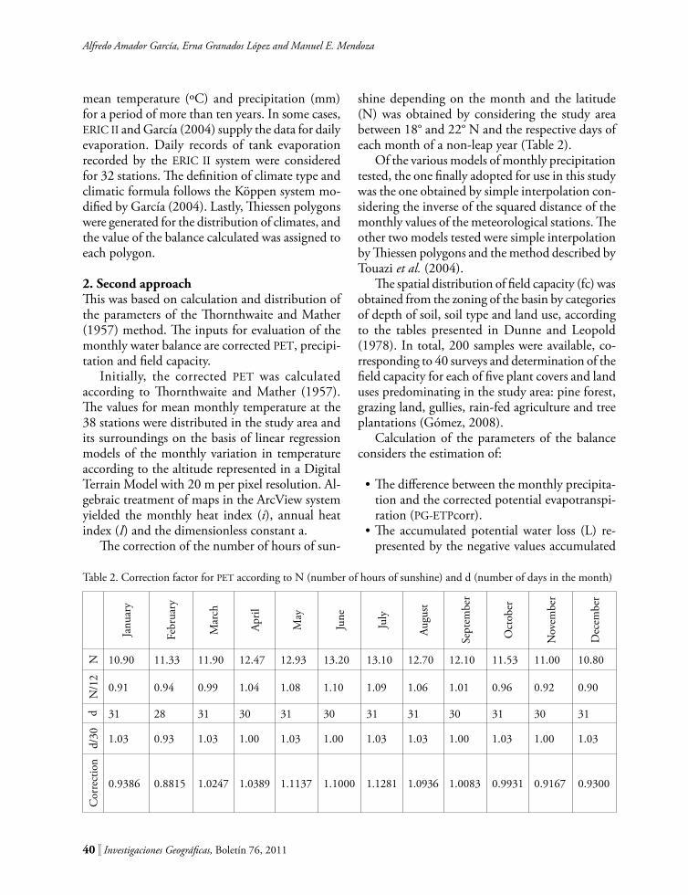
shine depending on the month and the latitude (N) was obtained by considering the study area between 18° and 22° N and the respective days of each month of a non-leap year (Table 2).

Of the various models of monthly precipitation tested, the one finally adopted for use in this study was the one obtained by simple interpolation con-sidering the inverse of the squared distance of the monthly values of the meteorological stations. The other two models tested were simple interpolation by Thiessen polygons and the method described by Touazi et al. (2004).

The spatial distribution of field capacity (fc) was obtained from the zoning of the basin by categories of depth of soil, soil type and land use, according to the tables presented in Dunne and Leopold (1978). In total, 200 samples were available, co-rresponding to 40 surveys and determination of the field capacity for each of five plant covers and land uses predominating in the study area: pine forest, grazing land, gullies, rain-fed agriculture and tree plantations (Gómez, 2008).

Calculation of the parameters of the balance considers the estimation of:

• The difference between the monthly precipita-tion and the corrected potential evapotranspi-ration (PG-ETPcorr).

• The accumulated potential water loss (L) re-presented by the negative values accumulated

Table 2. Correction factor for PET according to N (number of hours of sunshine) and d (number of days in the month)

Janu

ary

Febr

uary

Mar

ch

April

May

June

July

Augu

st

Sept

embe

r

Oct

ober

Nov

embe

r

Dec

embe

r

N 10.90 11.33 11.90 12.47 12.93 13.20 13.10 12.70 12.10 11.53 11.00 10.80

N/1

2

0.91 0.94 0.99 1.04 1.08 1.10 1.09 1.06 1.01 0.96 0.92 0.90

d 31 28 31 30 31 30 31 31 30 31 30 31

d/30 1.03 0.93 1.03 1.00 1.03 1.00 1.03 1.03 1.00 1.03 1.00 1.03

Cor

rect

ion

0.9386 0.8815 1.0247 1.0389 1.1137 1.1000 1.1281 1.0936 1.0083 0.9931 0.9167 0.9300



month by month. The value 0 is assigned to the first month in which the PG is greater than

the PETcorr at the end of the rainy season; a value equal to the field capacity is assigned to the first

month in which the PG is greater than the PETcorr at the beginning of the rainy season.

• The moisture retained in the soil (SM). Of the various ways by which this parameter can be evaluated (Dunne and Leopold, 1978), em-pirically Campos (1992) shows that it can be estimated by means of the formula:

SM= fc*e L/fc (2)

where SM is the soil moisture, fc the field capa-city, e is 2.7182 and L the loss of water potentially accumulated.

The change in soil moisture (∆SM) resumes in the last month in which the PETcorr is less than the PG, and this month is assigned the value 0. The later months are calculated as the difference between SM of the present month and SM of the preceding month. For months in which PG>PETcorr, ∆SM equals the difference between PG and PETcorr.

To complete and obtain the principal products of the balance the following parameters are obtained:

• Actual evapotranspiration (AET). This equals the difference between PG and ∆SM, except for those months in which ETPcorr is less than PG, and in those cases ETR equals ETPcorr.

• Soil Moisture Deficit (SMD). Although con-ceptually this corresponds to the water that a crop would require during those months for its maintenance, in practical terms it corresponds to the difference between ETPcorr and ETR.

• Water Surplus (WS). This parameter represents the amount of water that can run off or perhaps infiltrate, and is calculated by

WS= PG-(∆SM+AET) (3)

Dunne and Leopold (1978) state that for large basins approximately 50% of the surplus water is available for runoff in any month. This assumption was applied in the present study.

3. Third approachThe inputs for this approach comprise the records from evaporation tanks available in 35 of the 38 stations, as well as the database for the land cover and land use (LCLU) for the year 2000 and the monthly maps of distribution of precipitation.

The daily values of tank evaporation were interpolated in the study area and converted to ET0 values by multiplication by the factor 0.65 as specified by FAO (1990). The daily maps were added together monthly to provide an estimate of the monthly reference evapotranspiration.

The monthly ET0 values are obtained from the multiplication of the monthly ET0 map and the spe-cific coefficient of the crop, or in this case of the plant cover (kc). Since the available map of land use and land cover specifies the various modalities of crops, plantations and types of vegetation, the next step was to rate these categories according to the FAO (1990) rationale. The distributed values according to the 42 categories of LCU recognized in 2000 by Mendoza et al. (2001) are shown in Table 3.

FAO (1990) proposed a method for estimating the mean runoff. However, with a focus on balance, the monthly values of ET0 and ETc must far exceed the values of PET and AET estimated by the method of Thornthwaite and Mather (1957), since a total comes from the ETc accumulated in the months of June to September (during which PG>ET). To this last is added the potential soil moisture retention shown in the map of field capacity (fc) and the positive values of the difference of this sum from the PG accumulated for these same months; these values are regarded as water surplus that possibly runs off in its entirety. In this way, consideration of retention of moisture in the soil is incorporated into defining the specific coefficient of the crop and into the sum with the ETc values, so that it is assumed that at the end of the rainy period it will reach field capacity.

4. Supplying the ET (ETR) values and execution of the HEC modelThe inputs for this other focus of the water balance in the basin are as follows: the spatial distribution of the ET values calculated by the two first approaches;



Mendoza (2010), and a surface area of 30 760 ha, so that the volume contained in the lake is estima-ted at 307.60 hm3. Previous studies have tested a relationship between the lake surface and climatic variables, particularly the previous precipitation (Mendoza et al., 2006).

RESULTS

1. First approachThe most common climate in the study area is type Cb (temperate with a long fresh summer), which occupies some 90% of the study area (Figure 2). This is followed by the semi-warm types (A)C and A(C) with a total of 6% of the area. Type Cc (semi-cold with cool summer) accounts for some 2% of the area, this being derived from analysis of the Los Azufres station to the east of the drainage divide within the study area. Finally, the arid type BS1 (the least arid of the BS types) accounts for a

USE OR COVER Kc USE OR COVER KcAquaculture 1.05Human settlements 1.00 Lakes 1.05Dams 1.20 Closed scrubland 1.20Open Abies woodland 1.00 Open scrubland grassland 1.20Closed Abies woodland 1.00 Semi-open scrubland grassland 1.20Semi-open Abies woodland 1.00 Closed grassland 0.75Open oak woodland 1.00 Halophyte pastures 1.20Closed oak woodland 1.00 Open tree plantations 1.05Semi-open oak woodland 1.00 Open eucalypt tree plantations 1.25Open pine woodland 1.00 Open pine tree plantations 1.00Closed pine woodland 1.00 Closed tree plantations 1.15Semi-open pine woodland 1.00 Closed eucalypt tree plantations 1.25Open mixed woodland 1.00 Closed pine tree plantations 1.00Closed mixed woodland 1.00 Semi-open tree plantations 1.15Semi-open mixed woodland 1.00 Semi-open eucalypt tree plantations 1.25Natural water bodies 1.05 Semi-open pine tree plantations 1.00Seasonal irrigated crops 1.15 Bare soils 1.20Seasonal irrigated crops in flood zones 1.15 Vacant land 1.20Seasonal crops in terraces 1.15 Aquatic vegetation (tule, carrizo [Phragmites communis]

and water lily)1.20

Rain-fed seasonal crops 1.15 Flood zones of dams 1.05Market gardens 1.15 Flood zones of the lake 1.05

Table 3. Categories of cover and land use in the basin in the year 2000 and values of the coefficient specific to crop (or cover) for calculating ET

the categorization of the values of the LCLUdatabase reclassified as a function of the Numeric Curve values (Table 4); and a time series of preci-pitation for 2004, compiled by means of an auto-mated mechanism of data storage at five-minute intervals, deployed at the drainage divide of the basin (San José de la Cumbre, Michoacán). This precipitation series was used because of the lack of series with this temporal detail in the ERIC II database. These inputs are fed into the HEC model and the simulation of storms and potential runoffs can proceed.

The three approaches to the water balance of the basin take for reference the area of the main water body, Lake Cuitzeo, defined by INEGI at a 1:50 000scale. If there is no available gauging station in the basin and consequently there are no records of flows, the surface of the lake is considered as a proxy for data from hydrologic gauges. A mean depth of 1 m is assumed, in accordance with the records of Mendoza et al. (2006) and Vekerdy and



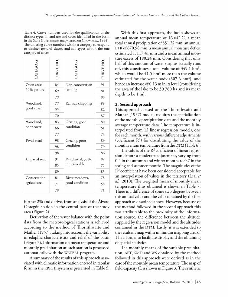
further 2% and derives from analysis of the Álvaro Obregón station in the central part of the study area (Figure 2).

Derivation of the water balance with the point data from the meteorological stations is achieved according to the method of Thornthwaite and Mather (1957), taking into account the variability in edaphic characteristics and relief of the basin (Figure 3). Information on mean temperature and monthly precipitation at each station is processed automatically with the WATBAL program.

A summary of the results of this approach asso-ciated with climatic information entered in tabular form in the ERIC II system is presented in Table 5.

CAT

EGO

RY

CU

RVE

NO

.

CAT

EGO

RY

CU

RVE

NO

.

Open areas 50% pasture

84 Non-conservation farming

91

69 81

79 88

Woodland, good cover

77 Railway chippings 89

55 82

70 87

Woodland, poor cover

83 Grazing, good condition

80

66 61

77 74

Paved road 98 Grazing, poor condition

89

98 79

98 86

Unpaved road 91 Residential, 38% impermeable

87

85 75

89 83

Conservation agriculture

81 River meadows, good condition

78

71 58

78 71

Table 4. Curve numbers used for the qualification of the distinct types of land use and cover identified in the basin in the State Government map (based on Chow et al., 1994). The differing curve numbers within a category correspond to distinct textural classes and soil types within the one category of cover

With this first approach, the basin shows an annual mean temperature of 16.64° C, a mean total annual precipitation of 851.22 mm, an annual ETR of 670.98 mm, a mean annual moisture deficit estimated at 117.41 mm and a mean annual mois-ture excess of 180.24 mm. Considering that only half of this amount of water surplus actually runs off, this constitutes a total volume of 349.1 hm3, which would be 41.5 hm3 more than the volume estimated for the water body (307.6 hm3), and hence an increase of 0.13 m in its level (considering the area of the lake to be 30 760 ha and its mean depth to be 1 m).

2. Second approachThis approach, based on the Thornthwaite and Mather (1957) model, requires the spatialization of the monthly precipitation data and the monthly average temperature data. The temperature is in-terpolated from 12 linear regression models, one for each month, with various different adjustments (coefficient R2) for distributing the value of the monthly mean temperature from the DTM (Table 6).

The values of the R2 coefficient of linear regres-sion denote a moderate adjustment, varying from 0.4 in the autumn and winter months to 0.7 in the spring and summer months. The magnitudes of the R2 coefficient have been considered acceptable for an interpolation of values in the territory (Leal et al., 2010). The weighted mean of monthly mean temperature thus obtained is shown in Table 7. There is a difference of some two degrees between this annual value and the value obtained by the first approach as described above. However, because of the method followed in the second approach this was attributable to the proximity of the informa-tion source, the difference between the altitude supplied by the regression model and the altitudes contained in the DTM. Lastly, it was extended to the resultant map with a minimum mapping area of 1 ha in order to facilitate display and the obtaining of spatial statistics.

The monthly means of the variable precipita-tion, AET, SMD and WS obtained by the method followed in this approach were derived as in the case of the monthly mean temperature. The map of field capacity (L is shown in Figure 3. The synthetic



101º 28' 39"

101º 29' 09"

101º 17' 13"

101º 17' 41"

101º 05' 47"

101º 06' 12"

100º 54' 21"

100º 54' 45"

100º 42' 55"

100º 43' 16"

100º 31' 29"

100º 31' 48"

19º 31' 41"19º 31' 04"

19º 41' 54"

19º 52' 44"

20º 03' 34"

19º 42' 32"

19º 53' 22"

20º 04' 13"

Basin

Water bodies

Sampling stations Thiessen

Scale

polygons

101º 28' 39"

101º 29' 09"

101º 17' 13"

101º 17' 41"

101º 05' 47"

101º 06' 12"

100º 54' 21"

100º 54' 45"

100º 42' 55"

100º 43' 16"

100º 31' 29"

100º 31' 48"

19º 31' 41"19º 31' 04"

19º 41' 54"

19º 52' 44"

20º 03' 34"

19º 42' 32"

19º 53' 22"

20º 04' 13"

Scale

Sampling stations

Basin

Water bodies

Field capacity (mm)

Figure 3. Distribution of the field capacity employed in the water balance of the basin.

Figure 2. Thiessen polygons for climates in the study area.



STATION No T PG E P/T ATO ET MD WSAcámbaro 1 18.3 780.1 1891.9 42.5 7.0 706.0 147.0 75.0Acuitzio del Canje 2 17.3 967.7 - - - - 55.8 6.2 732.0 75.0 236.0Álvaro Obregón 3 19.4 595.4 - - - - 30.6 7.0 596.0 311.0 0.0Carrillo Puerto 4 16.5 695.0 1979.6 42.1 6.9 648.0 129.0 47.0Cerano 5 18.8 797.7 1762.5 42.5 7.6 739.0 139.0 59.0Chucándiro, Chucándiro 6 14.3 823.9 1526.0 57.8 7.7 638.0 72.0 186.0Coinzio reservoir 7 16.7 849.3 1703.8 51.0 6.6 663.0 117.0 187.0Copándaro de Galeana 8 15.3 814.5 1788.4 53.4 7.0 636.0 101.0 178.0Cuitzeo del Porvenir 9 17.8 752.3 1695.1 42.3 7.0 686.0 138.0 66.0Cuitzillo Grande 10 16.8 659.3 1855.4 39.3 6.9 660.0 126.0 0.0Temazcal, El 11 16.6 1499.9 1141.5 90.2 5.4 676.0 98.0 824.0Huaniqueo, Huaniqueo 12 12.5 855.6 1416.0 68.3 9.1 614.0 53.0 241.0Huingo 13 17.2 778.4 1957.7 45.3 6.9 674.0 129.0 105.0Iramuco 14 17.7 723.6 1414.3 41.0 7.2 680.0 142.0 44.0Jesús del Monte 15 17.9 810.9 - - - - 45.2 6.7 664.0 164.0 146.0Huerta, La 16 17.0 868.2 - - - - 51.0 6.6 684.0 113.0 184.0Azufres, Los 17 10.7 1437.4 1157.5 134.5 5.4 602.0 22.0 836.0Molinos de Caballero 18 14.6 941.2 - - - - 64.6 6.4 650.0 64.0 291.0Morelia II 19 17.7 794.1 1707.7 44.7 6.8 701.0 123.0 93.0Moroleón 20 19.4 829.6 1993.7 42.7 7.0 739.0 170.0 91.0Pátzcuaro 21 16.2 930.0 1398.0 57.5 6.6 665.0 98.0 265.0Zinzimeo 22 17.1 800.0 2227.0 46.7 7.2 665.0 136.0 135.0Agostitlán reservoir 23 14.0 1360.9 1249.5 97.1 5.2 661.0 37.0 699.0Malpaís reservoir 24 17.2 701.6 1755.0 40.7 6.6 673.0 131.0 28.0Pucuato, reservoir 25 13.4 1328.3 1223.2 99.4 5.3 648.0 34.0 680.0Sabaneta, reservoir 26 13.6 1350.2 1218.6 99.4 5.4 655.0 32.0 695.0Puruándiro 27 19.2 857.6 2305.1 44.6 7.2 732.0 162.0 125.0Quirio 28 17.7 750.7 1558.7 42.4 7.1 682.0 141.0 68.0San Miguel del Monte 29 15.6 957.3 1429.9 61.3 5.9 629.0 114.0 328.0San Sebastián 30 16.4 669.2 1943.5 40.9 7.0 654.0 120.0 16.0Santa Fe Quiroga 31 17.1 1043.5 1536.7 61.0 5.9 690.0 105.0 354.0Santiago Undameo 32 15.7 881.3 1180.8 56.2 6.9 670.0 80.0 211.0Solís, reservoir 33 18.6 762.2 1638.1 40.9 7.0 724.0 142.0 38.0Santa Rita 34 21.0 729.8 2130.9 34.7 6.8 730.0 271.0 0.0Trinidad Hacienda 35 14.7 1117.4 - - - - 76.0 6.5 658.0 60.0 459.0Tzitzio (Alto Lerma) 36 21.0 1298.6 1619.2 61.7 5.6 807.0 192.0 491.0Villa Madero 37 15.5 1251.8 1206.3 80.8 5.8 663.0 76.0 589.0Zinapécuaro 38 17.3 761.5 1452.0 44.1 7.4 662.0 144.0 99.0

T (mean annual temperature) and ATO (annual thermal oscillation) in °C; PG (precipitation), E (evaporation), AET (actual evapotranspiration), MD (spoil moisture deficit) and WS (water surplus) in mm; P/T in mm/°C.

Table 5. Annual values of inputs and results of the water balance in the stations with available information



MONTH MODEL R2

JAN y = -0.0049x + 22.981 0.436

FEB y = -0.0057x + 25.531 0.368

MAR y = -0.0066x + 29.837 0.420

APR y = -0.0071x + 32.853 0.459

MAY y = -0.0075x + 34.819 0.539

JUN y = -0.0069x + 33.072 0.634

JUL y = -0.0068x + 31.754 0.648

AUG y = -0.0065x + 31.031 0.647

SEPT y = -0.0062x + 30.18 0.617

OCT y = -0.006x + 28.686 0.480

NOV y = -0.0055x + 26.061 0.339

DEC y = -0.0051x + 23.834 0.339

Table 6. Linear regression models of altitude (x, in m) v. mean monthly temperature (y, in degrees Centigrade)

Table 7. Weighted mean by surface area, of the monthly mean temperatures (°C) modelled for the basin

MO

NT

H

MEA

N

MIN

IMU

M

MEA

N

MAX

IMU

M

RAN

GE

WEI

GH

TED

M

EAN

STAN

DAR

D

DEV

IAT

ION

JAN 8.25 16.02 7.77 13.16 0.83

FEB 8.23 16.55 8.32 13.60 0.93

MAR 8.93 17.86 8.94 14.80 1.03

APR 9.62 18.91 9.28 15.78 1.09

MAY 9.96 19.52 9.56 16.35 1.14

JUN 10.06 19.20 9.15 16.10 1.07

JUL 9.56 18.64 9.08 15.55 1.06

AUG 9.69 18.55 8.87 15.50 1.02

SEPT 9.75 18.41 8.66 15.39 0.98

OCT 9.32 17.85 8.52 14.86 0.96

NOV 8.82 17.00 8.18 14.07 0.90

DEC 8.35 16.26 7.90 13.38 0.86

ANNUAL 14.88

Table 8. Weighted mean by surface area of the main parameters of the outcome of the water balance (mm) of the basin according to the first approach. The water surplus is shown at 50% of the total estimated here in order to make it equivalent to the runoff

MO

NT

H

PG ET SMD

WS(

Q)

JAN 15.35 35.34 9.71 0.00

FEB 7.46 28.55 15.84 0.00

MAR 6.82 30.58 27.98 0.00

APR 13.77 32.05 33.26 0.00

MAY 41.65 50.78 22.98 0.00

JUN 139.37 71.24 0.00 34.06

JUL 194.90 69.36 0.00 62.77

AUG 179.10 66.94 0.00 56.08

SEPT 151.38 61.06 0.00 45.16

OCT 63.15 56.49 0.57 0.00

NOV 14.61 46.73 1.85 0.00

DEC 9.84 38.39 7.34 0.00

ANNUAL 837.40 587.53 119.52 198.07

results for monthly balance for the whole of the basin are shown in Table 8.

With the second approach, the basin shows an annual mean temperature of 14.88° C, a mean total annual precipitation of 837.4 mm, an annual ETR of 587.53 mm, an annual mean moisture deficit estimated at 119.52 mm and an annual mean excess of moisture of 249.87 mm. Considering 50% of this last value as annual mean runoff, as cited by Dunne and Leopold (1978), 50% of the value of WS obtained by the Thornthwaite and Mather is distributed on an area of 387,382 Ha corresponding to a volume of 767.2 Mm3. As previously stated, a lake surface of approximately 30,760 Ha and 1 m in depth contains a volume of 307.6 Mm3.

3. Third approachThe principal product of this approach was achie-ved thanks to the detailed map of land use cover (Mendoza et al., 2001). The various categories of



this layer accounted for areas within the basin in the year 2000 as shown in Table 9.

Among the parameters required for the FAO-Penman equation (FAO 1990), some are difficult to find monitored in the conventional meteorological stations administrated by the Comisión Nacional del Agua (CNA). However, a variant of the method recommended by FAO itself allows the equation to be fulfilled either by approximation by the method of Hargreaves (1983) or from the coefficient of tank evaporation. In the former case, Hargreaves (1983) requires estimations of minimum tempe-rature, maximum temperature and extraterrestrial radiation. Extraterrestrial radiation is not difficult to estimate; however, although the linear regression models showed the possibility of a relationship with the values of altitude in the basin for the maximum

temperature this was not the case for the minimum temperature (Table 10).

Following from the above, the FAO-Penman method (FAO 1990) was followed as stipulated in the FAO manual, calculating the value of the reference evapotranspiration (ET0) with the data observed in the evaporation tank, as outlined in the Methods section above. The interpolation of these ET0 values multiplied by the crop coefficient (in this case also the coefficient of cover) allowed the monthly ETc values to be obtained and dis-tributed.

Unlike the method used in the second ap-proach, these maps (Figures 4 and 5) did not consider the retention and use of soil moisture by the crop or the type of cover during the months in which the ETc is less than PG.

Table 9. Surface area (ha) of soil use and soil cover in the basin in 2000

USE OR COVER ha USE OR COVER ha

Aquaculture 30.6 Lakes 30760.9

Human settlements 15093.7 Closed scrubland 32322.1

Dams 1102.4 Open scrubland 27665.8

Open Abies woodland 124.7 Open scrubland grassland 80.8

Closed Abies woodland 54.8 Semi open scrubland grassland 32926.6

Semi-open Abies woodland 135.8 Closed grassland 21391.4

Open oak woodland 5514.4 Halophyte pastures 3971.7

Closed oak woodland 10617.8 Open tree plantations 251.8

Semi-open oak woodland 9132.1 Open eucalypt tree plantations 797.7

Open pine woodland 50.0 Open pine tree plantations 7.5

Closed pine woodland 865.2 Closed tree plantations 346.2

Semi-open pine woodland 3082.6 Closed eucalypt tree plantations 606.9

Open mixed woodland 4881.6 Closed pine tree plantations 406.2

Closed mixed woodland 35089.3 Semi-open tree plantations 699.7

Semi-open mixed woodland 7334.3 Semi-open eucalypt tree plantations 1084.4

Natural water bodies 233.0 Semi-open pine tree plantations 51.7

Seasonal irrigated crops 47974.8 Bare soil 921.1

Seasonal irrigated crops in flood zones 2439.6 Vacant land 2865.7

Seasonal crops in terraces 4246.9 Aquatic vegetation (tule, carrizo [Phragmites communis] and water lily) 5640.6

Rain-fed seasonal crops 72141.4 Flood zones of dams 32.0

Market gardens 2683.7 Flood zones of the lake 1722.4



Table 10. Linear regression models of altitude (x, in m) v. maximum and minimum monthly temperatures (y, in degrees Centigrade)

MONTH maximum R2 minimum R2

January y = -0.007x + 36.405 0.6122 y = -0.0044x + 13.622 0.2475

February y = -0.0075x + 38.685 0.6367 y = -0.0046x + 14.82 0.2268

March y = -0.0076x + 41.519 0.6259 y = -0.0056x + 18.705 0.3282

April y = -0.0083x + 44.869 0.6182 y = -0.0061x + 21.839 0.3662

May y = -0.0091x + 46.976 0.7208 y = -0.0064x + 24.252 0.5256

June y = -0.009x + 44.326 0.7731 y = -0.0057x + 24.083 0.644

July y = -0.0085x + 41.3 0.7551 y = -0.0056x + 23.594 0.7482

August y = -0.0081x + 40.566 0.7433 y = -0.0055x + 23.146 0.7286

September y = -0.0079x + 39.937 0.7182 y = -0.0052x + 22.348 0.7011

October y = -0.0076x + 39.42 0.7005 y = -0.0047x + 19.362 0.4777

November y = -0.0073x + 38.08 0.6529 y = -0.0043x + 15.785 0.2453

December y = -0.0072x + 36.806 0.6420 y = -0.0036x + 12.994 0.1683

The ETc values obtained are much higher than those corresponding to PET and AET. Since this is a method for estimating evapotranspiration and not the water balance itself, an amount of potential loss of water is not considered for the months in which ETc is greater than PG.

ETc is greater than PG in the months without precipitation, and the weighted means by area of ETc are less in the rainy months than in the months preceding them (Table 11). Hence, it is not possible to use the maps of these evaluated parameters to obtain a direct algebraic estimate of the water surplus.

The rainy months (June, July, August and September) were grouped in order to obtain the accumulated amount for PG and to subtract it in its turn from the ETc accumulated for these same months from the map of field capacity. The above was based on the assumption that it would reach the field capacity at the end of the rainy period (Figure 6).

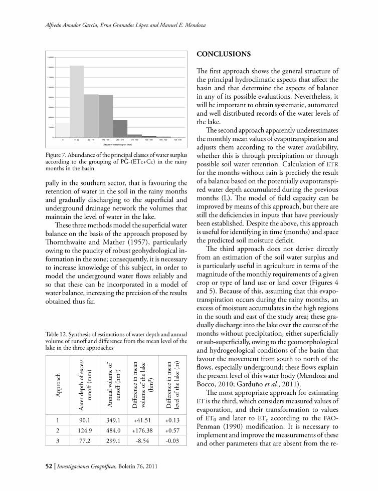
The water surplus in the basin that is not retai-ned by the field capacity increases cumulatively du-ring the rainy months to a total weighted by surface average of 77.2 mm. The frequency histogram co-rresponding to the values in the distribution map of water surplus estimated by this aggregation is shown in Figure 7. It is noteworthy that the FAO-Penman

approach results in a weighted by surface average water flow volume of 229.05 Mm3. Such volume is only 8.5 Mm3 less than the estimated flow needed for maintaining a depth of 1 m in lake Cuitzeo, a difference that would represent an eventual fluc-tuation of 2 cm in the average lake’s surface level.

DISCUSSION

The weighted mean of tessellated surface of the parameters of water balance yields a first scenario of the annual means around which the climatic characteristics and the water balance of the basin fluctuate. A 50% retention of the water surplus in the basin would represent an annual increase of only 13.5 cm in the mean level of water (Table 12). The evident disadvantage of this approach lies in the impossibility of the identification of critical areas with moisture deficit throughout the year, sin-ce tessellation only distributes geometrically with the crossing of perpendicular bisectors uniform values that do not take into account functions of proximity nor of altitudinal variation of the para-meters involved.

With the approach based on the Thornthwaite method, consideration of only half the water sur-plus involves an increment of up to 0.57 m in the



Figu

re 4

. Esti

mat

ed m

onth

ly e

vapo

tran

spira

tion

(ET,

mm

) of ‘

crop

’ (or

cov

er),

Janu

ary

to Ju

ne.

101º

28'

39"

101º

29'

09"

101º

17'

13"

101º

17'

41"

101º

05'

47"

101º

06'

12"

100º

54'

21"

100º

54'

45"

100º

42'

55"

100º

43'

16"

100º

31'

29"

100º

31'

48"

19º 3

1' 4

1"19

º 31'

04"

19º 4

1' 5

4"

19º 5

2' 4

4"

20º 0

3' 3

4"

19º 4

2' 3

2"

19º 5

3' 2

2"

20º 0

4' 1

3"

101º

28'

39"

101º

29'

09"

101º

17'

13"

101º

17'

41"

101º

05'

47"

101º

06'

12"

100º

54'

21"

100º

54'

45"

100º

42'

55"

100º

43'

16"

100º

31'

29"

100º

31'

48"

19º 3

1' 4

1"19

º 31'

04"

19º 4

1' 5

4"

19º 5

2' 4

4"

20º 0

3' 3

4"

19º 4

2' 3

2"

19º 5

3' 2

2"

20º 0

4' 1

3"

101º

28'

39"

101º

29'

09"

101º

17'

13"

101º

17'

41"

101º

05'

47"

101º

06'

12"

100º

54'

21"

100º

54'

45"

100º

42'

55"

100º

43'

16"

100º

31'

29"

100º

31'

48"

19º 3

1' 4

1"19

º 31'

04"

19º 4

1' 5

4"

19º 5

2' 4

4"

20º 0

3' 3

4"

19º 4

2' 3

2"

19º 5

3' 2

2"

20º 0

4' 1

3"

101º

28'

39"

101º

29'

09"

101º

17'

13"

101º

17'

41"

101º

05'

47"

101º

06'

12"

100º

54'

21"

100º

54'

45"

100º

42'

55"

100º

43'

16"

100º

31'

29"

100º

31'

48"

19º 3

1' 4

1"19

º 31'

04"

19º 4

1' 5

4"

19º 5

2' 4

4"

20º 0

3' 3

4"

19º 4

2' 3

2"

19º 5

3' 2

2"

20º 0

4' 1

3"

101º

28'

39"

101º

29'

09"

101º

17'

13"

101º

17'

41"

101º

05'

47"

101º

06'

12"

100º

54'

21"

100º

54'

45"

100º

42'

55"

100º

43'

16"

100º

31'

29"

100º

31'

48"

19º 3

1' 4

1"19

º 31'

04"

19º 4

1' 5

4"

19º 5

2' 4

4"

20º 0

3' 3

4"

19º 4

2' 3

2"

19º 5

3' 2

2"

20º 0

4' 1

3"

101º

28'

39"

101º

29'

09"

101º

17'

13"

101º

17'

41"

101º

05'

47"

101º

06'

12"

100º

54'

21"

100º

54'

45"

100º

42'

55"

100º

43'

16"

100º

31'

29"

100º

31'

48"

19º 3

1' 4

1"19

º 31'

04"

19º 4

1' 5

4"

19º 5

2' 4

4"

20º 0

3' 3

4"

19º 4

2' 3

2"

19º 5

3' 2

2"

20º 0

4' 1

3"

Sam

plin

g st

atio

nsBa

sin

Wat

er b

odie

s

ET (m

m)

25-5

0

50-

7575

-100

10

0-12

512

5-15

015

0-17

517

5-20

020

0-22

522

5-25

0

June

Janu

ary

Febr

uary

Mar

ch

Apr

ilM

ay



101º

28'

39"

101º

29'

09"

101º

17'

13"

101º

17'

41"

101º

05'

47"

101º

06'

12"

100º

54'

21"

100º

54'

45"

100º

42'

55"

100º

43'

16"

100º

31'

29"

100º

31'

48"

19º 3

1' 4

1"19

º 31'

04"

19º 4

1' 5

4"

19º 5

2' 4

4"

20º 0

3' 3

4"

19º 4

2' 3

2"

19º 5

3' 2

2"

20º 0

4' 1

3"

101º

28'

39"

101º

29'

09"

101º

17'

13"

101º

17'

41"

101º

05'

47"

101º

06'

12"

100º

54'

21"

100º

54'

45"

100º

42'

55"

100º

43'

16"

100º

31'

29"

100º

31'

48"

19º 3

1' 4

1"19

º 31'

04"

19º 4

1' 5

4"

19º 5

2' 4

4"

20º 0

3' 3

4"

19º 4

2' 3

2"

19º 5

3' 2

2"

20º 0

4' 1

3"

101º

28'

39"

101º

29'

09"

101º

17'

13"

101º

17'

41"

101º

05'

47"

101º

06'

12"

100º

54'

21"

100º

54'

45"

100º

42'

55"

100º

43'

16"

100º

31'

29"

100º

31'

48"

19º 3

1' 4

1"19

º 31'

04"

19º 4

1' 5

4"

19º 5

2' 4

4"

20º 0

3' 3

4"

19º 4

2' 3

2"

19º 5

3' 2

2"

20º 0

4' 1

3"

101º

28'

39"

101º

29'

09"

101º

17'

13"

101º

17'

41"

101º

05'

47"

101º

06'

12"

100º

54'

21"

100º

54'

45"

100º

42'

55"

100º

43'

16"

100º

31'

29"

100º

31'

48"

19º 3

1' 4

1"19

º 31'

04"

19º 4

1' 5

4"

19º 5

2' 4

4"

20º 0

3' 3

4"

19º 4

2' 3

2"

19º 5

3' 2

2"

20º 0

4' 1

3"

101º

28'

39"

101º

29'

09"

101º

17'

13"

101º

17'

41"

101º

05'

47"

101º

06'

12"

100º

54'

21"

100º

54'

45"

100º

42'

55"

100º

43'

16"

100º

31'

29"

100º

31'

48"

19º 3

1' 4

1"19

º 31'

04"

19º 4

1' 5

4"

19º 5

2' 4

4"

20º 0

3' 3

4"

19º 4

2' 3

2"

19º 5

3' 2

2"

20º 0

4' 1

3"

101º

28'

39"

101º

29'

09"

101º

17'

13"

101º

17'

41"

101º

05'

47"

101º

06'

12"

100º

54'

21"

100º

54'

45"

100º

42'

55"

100º

43'

16"

100º

31'

29"

100º

31'

48"

19º 3

1' 4

1"19

º 31'

04"

19º 4

1' 5

4"

19º 5

2' 4

4"

20º 0

3' 3

4"

19º 4

2' 3

2"

19º 5

3' 2

2"

20º 0

4' 1

3"

Sam

plin

g st

atio

nsBa

sin

Wat

er b

odie

s

ET (m

m)

25-5

0

50-

7575

-100

10

0-12

512

5-15

015

0-17

517

5-20

020

0-22

522

5-25

0

July

Aug

ust

Sept

embe

r

Oct

ober

Nov

embe

rD

ecem

ber

Figu

re 5

. Esti

mat

ed m

onth

ly e

vapo

tran

spira

tion

(ET,

mm

) of ‘

crop

’ (or

cov

er),

July

to D

ecem

ber.



PG ETc

MONTH MEAN MEAN

January 15.35 74.06

February 7.46 89.92

March 6.82 131.24

April 13.77 151.27

May 41.65 146.16

June 139.37 113.50

July 194.90 94.43

August 179.10 93.41

September 151.38 84.57

October 63.15 84.39

November 14.61 72.41

December 9.84 74.82

Annual 837.40 1210.18

Table 11. Temporal distribution of the ETc values obtained by the third approach

101º 28' 39"

101º 29' 09"

101º 17' 13"

101º 17' 41"

101º 05' 47"

101º 06' 12"

100º 54' 21"

100º 54' 45"

100º 42' 55"

100º 43' 16"

100º 31' 29"

100º 31' 48"

19º 31' 41"19º 31' 04"

19º 41' 54"

19º 52' 44"

20º 03' 34"

19º 42' 32"

19º 53' 22"

20º 04' 13" Potential water surplus (mm)

Sampling stations

Basin

Water bodies

Scale

mean level of the lake (Table 12); this is completely unacceptable given the field observations of the le-vel of this body of water annually or in recent years in which, far from such a marked rise in level, there have been years during which the lake has dried up (Alvarado et al., 1994; Mendoza et al., 2006).

Despite the above, the strength of the second approach lies in the identification of areas with relatively high AET in the months without rain and therefore the zones in which the deficit of moisture represents a limitation for the various activities that require water.

Accepting in a preliminary way the appropriate-ness of the third approach in terms of mass balance would explain the maintenance of a highly frag-mented and diversified LCLU in the basin; despite the reduction in plant mass and despite conditions that decrease the ET and consequently increase Q, this does not increase sedimentation or raise excessively from year to year the mean level of the lake surface. In consequence, it is the mass of native vegetation of the basin and their less fragmented condition in the high parts of the basin, princi-

Figure 6. Excess moisture accumulated in the rainy months (June to September), estimated considering the distribution of the field capacity in the basin.



pally in the southern sector, that is favouring the retention of water in the soil in the rainy months and gradually discharging to the superficial and underground drainage network the volumes that maintain the level of water in the lake.

These three methods model the superficial water balance on the basis of the approach proposed by Thornthwaite and Mather (1957), particularly owing to the paucity of robust geohydrological in-formation in the zone; consequently, it is necessary to increase knowledge of this subject, in order to model the underground water flows reliably and so that these can be incorporated in a model of water balance, increasing the precision of the results obtained thus far.

CONCLUSIONS

The first approach shows the general structure of the principal hydroclimatic aspects that affect the basin and that determine the aspects of balance in any of its possible evaluations. Nevertheless, it will be important to obtain systematic, automated and well distributed records of the water levels of the lake.

The second approach apparently underestimates the monthly mean values of evapotranspiration and adjusts them according to the water availability, whether this is through precipitation or through possible soil water retention. Calculation of ETR for the months without rain is precisely the result of a balance based on the potentially evapotranspi-red water depth accumulated during the previous months (L). The model of field capacity can be improved by means of this approach, but there are still the deficiencies in inputs that have previously been established. Despite the above, this approach is useful for identifying in time (months) and space the predicted soil moisture deficit.

The third approach does not derive directly from an estimation of the soil water surplus and is particularly useful in agriculture in terms of the magnitude of the monthly requirements of a given crop or type of land use or land cover (Figures 4 and 5). Because of this, assuming that this evapo-transpiration occurs during the rainy months, an excess of moisture accumulates in the high regions in the south and east of the study area; these gra-dually discharge into the lake over the course of the months without precipitation, either superficially or sub-superficially, owing to the geomorphological and hydrogeological conditions of the basin that favour the movement from south to north of the flows, especially underground; these flows explain the present level of this water body (Mendoza and Bocco, 2010; Garduño et al., 2011).

The most appropriate approach for estimating ET is the third, which considers measured values ofevaporation, and their transformation to valuesof ET0 and later to ETc according to the FAO-Penman (1990) modification. It is necessary to implement and improve the measurements of these and other parameters that are absent from the re-

Table 12. Synthesis of estimations of water depth and annual volume of runoff and difference from the mean level of the lake in the three approaches

Appr

oach

Aate

r dep

th o

f exc

ess

runo

ff (m

m)

Annu

al v

olum

e of

ru

noff

(hm

3 )

Diff

eren

ce in

mea

n vo

lum

e of

the

lake

(h

m3 )

Diff

eren

ce in

mea

n le

vel o

f the

lake

(m)

1 90.1 349.1 +41.51 +0.13

2 124.9 484.0 +176.38 +0.57

3 77.2 299.1 -8.54 -0.03

0

20000

40000

60000

80000

100000

120000

140000

160000

- 0 0 - 20 20 - 140 140 - 160 260 - 370 370 - 490 490 - 600 600 - 720 720 - 840

Classes of water surplus (mm)

Figure 7. Abundance of the principal classes of water surplus according to the grouping of PG-(ETc+Cc) in the rainy months in the basin.



cords of the meteorological stations (for example, wind speed) with the aim of a better determination and spatio-temporal distribution of the ETc values. However, the final approach (the simulation) could be improved if there were hydrometeorological parameters that allowed calibration of the HEC model and the other spatially distributed hydro-logic model.

The ET values obtained by any of these three approaches must be evaluated on the basis of values of runoff measured via a system of hydrometric monitoring of the basin (at least 73 possible sites of gauging were identified); here would be recorded data that would allow initial assessment of the cau-ses and effects of the spatio-temporal modifications of the various parameters of water balance.

Of the three models used to simulate flows and estimate heights of the lake, the HEC model represents a viable alternative to the hydrological modelling of the basin, since it yielded the best estimates when the mean height of the lake (1 m) was compared with the result of calculation from modelling the flows of water by the three methods. In essence, the three models used here require the same quantity of data, the only ones available in the greater part of the national territory or in developing countries, with closed basins and lakes in their low-lying regions that allow the results of the modelling to be compared; this favours their reproducibility and their use in decision making.

ACKNOWLEDGMENTS

The authors acknowledge the support of the project Evaluación espacial y multitemporal de los cambios de cobertura y uso del terreno en la cuenca del lago de Cuitzeo: implicaciones para la sucesión forestal y el mantenimiento de la diversidad vegetal (DGAPA-PAPIIT, UNAM). We also acknowledge the constructive comments of the two anonymous re-viewers; finally, we thank Teodoro Carlón, Antonio Navarrete and Hugo Zavala for technical assistance.

REFERENCES

Alvarado Díaz, J., T. Zubieta Rojas, R. Ortega Murillo, A. Chacón Torres and R. Espinoza Gómez (1994), Hipertroficación en un lago tropical somero (lago de Cuitzeo, Michoacán, México), en Comisión de Ecolo-gía del H. Congreso de Michoacán LXVI Legislatura, El deterioro ambiental, de la cuenca del lago de Cuit-zeo, H. Congreso del Estado de Michoacán, México.

Campos Aranda, D. F. (1992), Procesos del Ciclo Hidroló-gico, Editorial Universitaria Potosina, San Luis Potosí, San Luis Potosí.

Carlón Allende, T., M. E. Mendoza, E. López Granados and L. M. Morales Manilla (2009), “Hydrogeogra-phical regionalisation: an approach for evaluating the effect of land cover change in watersheds. A case study in Cuitzeo Lake watershed, Mexico”, Water Resources Management, vol. 23, no. 12, pp. 2587-2603.

Chow, V. T., D. R. Maidment and L. W. Mays (1994), Hidrología Aplicada, McGrawHill, México.

Doorenbos, J. and W. O. Pruitt (1977), Crop water re-quirements, FAO Estudio de Riego y Drenaje, no.24, (rev.), FAO, Roma.

Dunne, T. and L. B. Leopold (1978), Water in envi-ronmental planning, W. H. Freeman and Co., San Francisco.

Elkaduwa, W. K. B and R. Sakthivadivel (1998), Use of historical data as a decision support tool in watershed management: a case study of the Upper Nilwala basin in Sri Lanka, Report 26, International Water Mana-gement Institute, Colombo, Sri Lanka.

ESRI (1999), ArcView 3.2, GIS, Environmental Systems Research Institute, Inc., New York.

FAO (1990), Evapotranspiración del cultivo: guías para la determinación de los requerimientos de agua de los cultivos, Estudio FAO Riego y Drenaje, no. 56.

Fuentes, J. J., M. Bravo and G. Bocco (2004), “Water balance and landscape degradation of an ungauged mountain watershed: case study of the Pico de Tan-cítaro National Park, Michoacán, Mexico”, Journal of Environmental Hydrology 12 5, Electronic Journal of the International Association for Environmental Hydrology [http://wwwhydrowebcom].

García, E. (2004), Modificaciones al Sistema de Clasifi-cación Climática de Köppen, Serie Libros, núm. 6, Instituto de Geografía, UNAM, México.

Garduño Monroy, V. H., V. H. Medina Vega, I. Israde Alcántara, V. M. Hernández Madrigal and J. A. Ávila Olivera (2011), “Unidades Geohidrológicas de la Región de Morelia-Cuitzeo”, in Cram, S., L. Galicia and I. Israde Alcántara (comps.), Atlas de la Cuenca del Lago de Cuitzeo: un análisis de la geografía del lago y su entorno socioambiental, Instituto de Geografía-



UNAM, Universidad Michoacana de San Nicolás de Hidalgo, México.

Gómez Tagle, Ch. A. (2008), Variabilidad de las pro-piedades edáficas relacionadas con la infiltración y la conductividad hidráulica superficial en la cuenca de Cuitzeo, tesis Doctoral, UMSNH, México.

Hargreaves, G. H. (1983), “Discussion of ‘Application of Penman wind function’ by Cuenca, R. H. and Nicholson, M.J. J. Irrig. and Drain. Engrg., ASCE 10, no. 2, pp. 277-278.

Hay, L. E., W. A. Battaglin and G. H. Leavesley (1993), “Modeling the effects of climate change on water resources in the Gunnison river basin, Colorado”, in Goodchild, M. F., B. O. Parks and L. T. Steyaert (eds.), Environmental modelling with GIS, pp. 172-181.

He, C., S. B. Macolm, K. A. Dahlberg and B. A. Fu (2000), “Conceptual framework for integrating hy-drological and biological indicators into watershed management”, Landscape and Urban Planning, no. 49,

pp. 25-34.HEC (2000), Geospatial Hydrologic Modeling Extension,

HEC-GEO-HMS, US Army Corps of Engineers, Hy-drologic Engineering Center, User’s Manual.

Hewlett, J. D. (1982), Principles of forest hydrology, Uni-versity of Georgia Press, Athens, Georgia.

IMTA (2000a), Sistema de Información Climatológica (SICLIM). 5319 Estaciones. Periodo 1921- 1990,

Base de datos [CD_ROM computer file], Morelos, México.

IMTA (2000b), Programa extractor rápido de información climática, ERIC versión 2.0, Instituto Mexicano de Tecnología del Agua, Base de datos [CD_ROM computer file], Morelos, México.

INEGI (1999), Conjunto de datos vectoriales, Instituto Nacional de Estadística, Geografía e Historia, México.

INEGI (1979, 1982, 1983), Mapas edafológicos, Insti-tuto Nacional de Estadística, Geografía e Historia, México.

Jensen, M. E. and H. R. Haise (1963), “Estimating evapotranspiration from solar radiation”, J. Irrig. and Drain., Div., ASCE, no. 89, pp. 15-41.

López Granados, E., G. Bocco, M. E. Mendoza, A. Veláz-quez and R. Aguirre (2006), “Peasant emigration and land-use change at the watershed level. A GIS-based approach in Central Mexico”, Agricultural Systems, vol. 90, no. 1-3, pp. 62-78.

López Granados, E., G. Bocco, M. E. Mendoza and E. Duhau (2001), “Predicting land-cover and land use change in the urban fringe. A case in Morelia city, Mexico”, Landscape and Urban Planning, vol. 55, no. 4,

pp. 271-285.Makkink, G. F. (1957), “Testing the Penman formula by

means of lysimeters”, J. Inst. Water Engng., vol. 11, no. 3, pp. 277-288.

Mendoza, M. E. and G. Bocco (2010), “Geomorfolo-gía”, in Cram, S., L. Galicia and I. Israde Alcántara (comps.), Atlas de la Cuenca del Lago de Cuitzeo: un análisis de la geografía del lago y su entorno socioam-biental, Instituto de Geografía-UNAM, Universidad Michoacana de San Nicolás de Hidalgo, México.

Mendoza, M. E., G. Bocco and M. Bravo (2002), “Spatial prediction in hydrology: status and implications in the estimation of hydrological processes for applied research”, Progress in Physical Geography, vol. 26, no. 3,

pp. 319-338.Mendoza, M. E., G. Bocco, E. López Granados and M.

Bravo (2010), “Hydrological implications of land-cover and land-use change: spatial analytical approach at regional scale in the closed basin of the Cuitzeo Lake, Michoacán, Mexico”, Singapore Tropical Geo-graphy, vol. 31, no. 2, pp.??

Mendoza, M. E., G. Bocco, M. Bravo, E. López Grana-dos and W. R. Osterkamp (2006), “Predicting water surface fluctuation of continental lakes. A GIS and RS based approach in Central Mexico”, Water Resources Management, vol. 20, no. 2, pp. 291-311.

Mendoza, M. E., E. López Granados and G. Bocco (2001), Regionalización ecológica, conservación de recursos y ordenamiento territorial, Informe Final presentado al Programa SIMORELOS–CONACYT, Departamento de Ecología de los Recursos Naturales, Instituto de Ecología, UNAM, México.

Monteith, J. L. (1965), “Evaporation and environment”, 19th Symposium of the Society for Experimental Biology, University Press, Cambridge, no. 19, pp. 205-234.

Neitsch, S. L., J. G. Arnold, J. R. Kiniry and J. R. Wi-lliams (2001), Soil and water assessment tool, theore-tical documentation, Texas Agricultural Experiment Station, Texas, USA.

Osman, B. E. T. (1996), GIS-hydrological modelling in arid lands: a geographical synthesis of surface waters for the African Dead Sea region in the Sudan, Doctoral thesis, Lund University, Sweden.

Penman, H. L. (1948), “Natural evaporation from open water, bare soil and grass”, Proc. Royal Society London, Ser. A, no. 193, pp. 120-148.

Priestley, C. H. B. and R. J. Taylor (1972), “On the as-sessment of surface heat flux and evaporation using large scale parameters”, Mon. Weath. Rev., no. 100, pp. 81-92.

SCS (1967), Soil Conservation Service, Irrigation Water Requirements, Technical Release No. 21, U. S. Dept. Agric., Engineering Div.

SCS (1972), Soil Conservation Service National En-gineering Handbook, Section on Hydrology, Soil Conservation Service, U.S. Dept. of Agriculture, Washington, D.C.



Thornthwaite, C. W. (1948), “An approach toward a rational classification of climate”, Geographic Review, no. 38, pp. 55-94.

Thornthwaite, C. W. and J. R. Mather (1957), Instruc-tions and Tables for Computing Potential Evapotranspi-ration and Water balance, Publications in Climatology 10(3), Drexel Institute for Technology, Laboratory of Climatology, Centerton, New Jersey.

Touazi, M., J. P. Laborde and N. Bhiry (2004), “Mode-lling rainfall-discharge at a mean inter-yearly scale in northern Algeria”, Journal of Hydrology, no. 296, pp. 179-191.

Turc, L. (1961), “Evaluation des besoins en eau d’irri-gation, évapotranspiration potentielle, formule climatique simplifiée et mise a jour”, Ann. Agron., no. 12, pp. 13-49.

Verkerdy, Z. and M. E. Mendoza (2010), “Batimetría. Dinámica del Lago de Cuitzeo”, in Cram, S., L. Galicia and I. Israde Alcántara (comps.), Atlas de la Cuenca del Lago de Cuitzeo: un análisis de la geogra-fía del lago y su entorno socioambiental, Instituto de Geografía-UNAM, Universidad Michoacana de San Nicolás de Hidalgo, México.

Ward, A. and A. Trimble (2003), Environmental hydro-logy, CRC Press, Boca Ratón.

Ziegler A. D., T. W. Giambelluca, D. Plondke, S. Leisz, L. T. Tran, J. Fox, M. A. Nullet, J. B. Vogler, D. M. Troung and T. Vien (2004), “Hydrological consequences of landscape fragmentation in mountainous northern Vietnam: evidence of accelerated overland flow gene-ration”, Journal of Hydrology, no. 287, pp. 124-146.

Zinck, J. A. (1988), Physiography and Soils, Soil Survey Course, ITC, Enschede, The Netherlands.

Three approaches to the assessment of spatio-temporal distribution … · los del escurrimiento se...

Documents

Transcript of Three approaches to the assessment of spatio-temporal distribution … · los del escurrimiento se...