Those with blue hair please step forward: An economic theory of group formation

and application to Cajas Rurales in Honduras

Carlos Elias and Jeffrey Alwang

Virginia Tech

CELIAS@VT.EDU

ALWANGJ@VT.EDU

Selected Paper prepared for presentation at the American Agricultural Economics

Association Annual Meeting, Orlando, FL, July 27-29, 2008.

Copyright 2008 by Carlos Elias and Jeffrey Alwang. All rights reserved. Readers may

make verbatim copies of this document for non-commercial purposes by any means,

provided that this copyright notice appears on all such copies.

The authors want to recognize Steve Buck for his outstanding work as the leader of the

team that executed lab experiments in the field. The authors also want to recognize the

logistical support provided by Luis Nunez of PRODERT and Sergio Cruz of ADIAC.

Finally the authors thank the BNPP Trust Fund, administered by the WB, for funding this

research project.

2

Abstract

This paper presents an economic model of group formation with an application to data

collected from an agricultural credit program in western Honduras. We formulate a

simple theory of group formation using the concept of centers of gravity to explain why

individuals join a group. According to our theory, prospective members join based on the

potential benefits and costs of group membership, and based on their perception of social

distance between themselves and other group members. Social distance is unobservable

by outsiders but known by the individual: if you are in then you know who has blue hair.

Thus, we argue that social distance helps explain preferences for group formation. To

test our theory we analyze data collected from members and non-members of PRODERT,

a program that has helped create 188 “Cajas Rurales” (CRs). Using conjoint analysis we

test for differences in preferences between members and non-members for the main

attributes of the CR. We find that members and non-members exhibit similar preferences

for the attributes of the CR; therefore non-membership is not related to supply factors.

Using information gathered by executing field experiments, we estimate a proxy for

social distance. We use this proxy to run a group formation equation and find that it

explains, along with individual characteristics, participation in the CR. Finally we offer

suggestions on how to balance performance and coverage in programs in which

beneficiaries decide who joins. Small cohesive groups may show exceptional

performance at the cost of low coverage, and the opposite may be true.

3

Introduction

The majority of the 700,000 people that live in the Trifinio Region—an area that

includes Guatemala, Honduras and El Salvador—are poor and do not have access to

opportunities that would allow them to climb out of poverty such as schools, health

programs, an established infrastructure system, or an effective legal system. The

challenges of this region have been recognized by the national governments of the

Trifinio and there is political will to address them. As a result of this will, the Trifinio

Commission was created in mid-1980s to coordinate efforts. The barriers for the

development of the region are formidable and according to the Trifinio Commission the

key is to break the vicious cycle of poverty-environmental degradation that characterizes

the socio-economic dynamic of this region. Many projects in execution in the Trifinio

address this issue; in this paper we focus on PRODERT Honduras, funded by Banco

Centroamericano de Integración Económica (BCIE).

The overall objective of PRODERT is to promote sustainable development of the

Trifinio by improving living conditions. More specifically, the project aims at: (i)

increasing productivity in agriculture and livestock activities, both for commercial

production and own consumption; (ii) improving infrastructure to facilitate trade; and (iii)

facilitating the creation of institutions that would, at the local level, make decisions about

development programs and provide services, including financing.

PRODERT Honduras decided early on that successful implementation of such an

ambitious program required the active participation and ownership of the project by its

participants. PRODERT packaged several components--financial and non-financial

4

services such as agricultural extension and housing improvements--and began to deliver

them to the poor through CR. By law each CR is independent and fully owned by its

members. NGOs are the link between each CR and PRODERT, and provide the

technical assistance that is at the core of this project.

With limited resources PRODERT decided to prioritize poor rural communities

that did not have support from other development programs. Initially PRODERT

approached municipal Mayors to identify communities in most need. With the Mayor’s

sponsorship PRODERT visited communities and conveyed a meeting to explain the

project. As a result of these meetings CR were created, with participation being

voluntary. As of April 2008 PRODERT has facilitated the creation of 188 CR that serve

over 3,850 families. In general CR are successful and are capitalizing rapidly. CR boast

perfect debt service performance as measured by arrears. The program, however, also

exhibits low coverage because on average membership includes only 30% of households

in each community.

Perfect performance combined with low coverage suggests that there is room to

increase coverage by balancing these competing objectives. PRODERT involved

prospective beneficiaries from the beginning, and delegated execution to “them.” But

who are “they”? We argue that the proper definition of “them” is complicated and goes

beyond the identification of the target population by observable selection criteria such as

income or education. We argue that this identification strategy is incomplete for

programs that require beneficiaries to cooperate and for outcomes that depend on

cooperation. We hypothesize that allowing for self selection in group formation means

5

members that join expect positive net benefits from joining and exhibit short social

distances between each other: the blue hair effect. Social distance is unobservable by

outsiders but observable to the individual: if you are in then you know who has blue hair.

Thus, we argue that social distance helps explain preferences for group formation.

This paper presents and tests an economic theory of group formation. The rest of

the paper includes a brief section on relevant literature that analyzes group formation,

social distance, and conjoint analysis. Then we present our theory of group formation

using social distance in a centers of gravity inspired model. Our research hypotheses and

data collection and hypotheses testing strategy is followed by a description of our data

and the main results of this paper, which then are summarized in the last section

presenting our recommendations for the design and implementation of development

programs that target poor rural farmers in Latin America.

Relevant literature

The question of group formation entered the lexicon of development economics in the

middle of the last century with Mancur Olson’s Logic of Collective Action, 1965. Since

that time the issue has branched off into directions such as the microcredit area with

detailed discussions of the experiences of the Grameen Bank (Stiglitz 1990). Multilateral

development organizations have increased their emphasis on group formation as

government planned and implemented programs have failed to provide the intended

economic boost. That is, there has been a marked increase in the use of the terms like

“participatory development” and “people-centered development,” which refer to

6

grassroots, decentralized development. This framework of development stresses the

participation of the people in the formulation of development policy.

Consider the following quote from James Wolfensohn, former World Bank President:

The lesson is clear: for economic advance, you need social advance, and

without social development, economic development cannot take root. … this

means that we need to make sure that the programs and projects we support

have adequate social foundations,

• by learning more about how the changing dynamics between public

institutions, markets, and civil society affect social and economic

development.

James Wolfensohn, speech at 1996 Annual Meetings.“New Paradigm” in

Summary Proceedings, 1996. P. 28.

And, in fact, there has been a clear push to broaden the community-driven

component of World Bank projects over the past 20 years—from 2% in 1989 to 25% in

2003 (WB2005). Unfortunately, recent studies have shown that encouraging local

communities to organize into groups that then have significant input into development

programs does not necessarily guarantee the success of the program for the community as

a whole. Frequently the “lead” group benefits while other members in the community

remain the same or end up even worse off (Walzer 2002). Moreover, there is evidence

that the more disadvantaged the individual, the less likely that person is to be a member

of a civic group. The causality (whether lack of participation limits progress or whether

lack of development prevents group entry) is not clear (Banfield 1958, Glaeser, Ponzetto,

and Schleifer 2006) but we do see that simply encouraging poor rural communities to

7

form groups is not enough to ensure that those communities will experience an across-

the-board improvement in living conditions.

What then can be done to broaden the impact of these rural community

development programs? Clearly the first step is to understand the dynamics of group

formation. This is particularly important when the program requires the participants

work together for the duration of the project implementation, not simply in the design and

conception phase. For example, Gugerty and Kremer (2006) found that as younger,

better-educated people joined the group, the disadvantaged members tended to exit.

Moreover, it was the new entrants, either male or educated female, who assumed key

leadership positions. In their study there was a two-thirds increase in the exit rate of

older women, the most disadvantaged demographic group, and a doubling of the rate at

which members left groups due to conflict.

Another way to describe the factors that can bring a group together (or force one

apart) is the “social distance” between the members. Striking the right balance in the

selection of program participants is conceptually appealing, but not easy to implement in

practice. The proper combination of attributes is crucial, and some of the traits may not

be readily observed by outsiders—although community members are likely to know

(Feder and Savastano 2006).

There is some evidence that microcredit institutions with outstanding repayment

records owe these rates to their small size and the effect of peer pressure that result from

it (Stiglitz 1990). In the case of PRODERT, however, the loans are individual rather than

group based so this effect should largely be mitigated. The conclusion we test is that the

8

CR will not expand beyond their current sizes due to the costs of entry related to social

distance rather than to a desire to remain small. We look to conjoint analysis to

demonstrate that no other difference is preferences can explain the barrier to entry.

Conjoint analysis (CA) is commonly used in commercial marketing studies and

analysis of consumers’ preferences. It evaluates consumer response to program attributes

when they are considered jointly. We use conjoint analysis to determine if there are

preference differences between members and non-members of the CRs. If so, these

differences might explain why the percentage of the community membership is not

higher. If there is no significant difference in preferences then another explanation (such

as social distance) must apply.

Dufhues, Heidhues, and Buchenreider (2004) conducted a similar test using the

same methods but we are working toward a different goal. We are measuring the

relevance of social distance in community members’ decisions to join the CR while they

are looking at ways to modify existing programs. The practical implications that are the

foundation of our paper imply that the perfect rural finance program might not appeal to

those community members that are not within the “gravity circle” of the existing

members. To provide a framework to analyze this issue we propose a theory of group

formation.

Theory of group formation

We formulate a simple theory of group formation using the concept of centers of

gravity to explain why individuals join a group. According to our theory, prospective

members join based on the potential benefits and costs of group membership, and based

9

on their perception of social distance between themselves and other group members.

Social distance is unobservable by outsiders but observable to the individual: if you are in

then you know who has blue hair. Thus, we argue that social distance helps explain

preferences for group formation.

We use the concept of social distance to account for the effect of “others” on the

individual’s decision to join a group. We modified the definition of social distance of

Hoffman, McCabe, Smith (1996) to read “the degree of reciprocity that subjects believe

exist within social space.” Hoffman et al uses “the degree of reciprocity that subjects

believe exist within a social interaction.” The modification is important because in the

context of group formation social distance does not depend on the particular social

interaction but social distance is inherited. People in social space interact with each other

and have definite perceptions about the degree of reciprocity between them. This

variation, in line with Akerlof (1997), implies that at any point in time there will be a

completely-defined set of social distances from any individual to the rest of people in the

community.

We use this initial set of social distances in social space to help explain group

formation. When a promoter attempts to form a group then she presents the group’s

purpose, objectives and characteristics to each individual who is invited to join. The

purpose, objectives and characteristics of the group are bundled in package x that is

defined by the attributes of the group. For example the attributes for the CR include

access to loans, extension services, and training; and obligations to contribute fees, save,

and participate in meetings. Each individual then analyses the costs and utility derived

10

from x in the context of the inherited set of social distance between the prospective

member and the promoters.

It is important to emphasize that x plays a central role in our theory of the impact

of social distance on group formation. For example when the cost-related attributes of x

are relaxed to x’, so that benefits increase with respect to costs, then additional

prospective members that with x had barely negative net benefits may now with x’ have

barely positive benefits, enough for some to join the group with the new attributes. In

this example the social distance of the new group members, that would join now with x’

but not with x, with respect to the promoters did not change because the attributes of x

changed. In other words the composition of the group is a consequence of the attributes

of x and x’.

We now formalize our theory of group formation. When an individual i is invited

to join a new group, her decision is influenced by her perceived benefits from joining the

group �����, inherited social distance to the center of gravity of the group promoters

(�� � ���, and perception of the costs of membership, ����. Such as Akerlof (1997) we

use the concept of gravitational pull to derive the functional form of the net benefits of

joining the group as directly proportional to the benefits of joining, and inversely

proportional to the square of the social distance to the center of gravity of group

promoters. The prospective member utility function of joining the group with bundled x

attributes is ����:

��� � �

�����

�� � ��������� (1)

11

Where:

� represents the bundled attributes of the group

����� is the utility function of individual i of joining group defined by attributes x

����� is the expected benefit to individual i of joining the group defined by attributes x

��� � ���� is the square of the social distance of individual i with respect to the center of

gravity of the promoters

�����

�������� is the formula for the pull force of gravity: the bigger the expected returns the

stronger the force is, the longer the social distance the weaker the pull force is to

individual i

����� is i’s perceived costs of joining the group

In this context for a group with attributes x individual i will join and j will not join

when:

���� � 0; ���� � 0 (2)

that may happen because:

�����, ���� � �����, ���� !� � "# ��$ � �%� � ��& � �%� (3)

This is the main result of our theory because we derive a condition for social

distance that is “sufficient” for joining a group given benefits and costs of group

membership. According to our theory members will join when their social distance to the

core of the group is small and when the benefits of joining are high compared to the

costs. Note that the first part of equation (3) is referring to differences in utility streams.

More people will join when the bundled x changes in a way that either benefits

increase—such as offering new non-financial services—or costs decrease—such as

12

reducing membership fees. Using another example additional supply of loans under

current lending terms will not increase membership, however changing lending terms

might. The intuition is straightforward, and is summarized Table 1.

Group formation hypotheses, data collection and testing strategy

Hypothesis 1: supply-side of group formation: community members have similar

preferences for the attributes of the CR

Hypothesis 2: demand side of group formation: using lab field experiments we

elicit a proxy for social distance and test for group formation

To test these 2 hypotheses we collected primary data. With PRODERT we

defined selection criteria for 5 CR in the municipalities of Concepcion and San Agustin,

Honduras. These 2 municipalities share the main characteristics of the target population

of PRODERT: most of the households are poor rural farmers living in relatively isolated

communities. In these 2 municipalities we selected 5 communities using the following

criteria: (i) communities of less than 200 households; (ii) agriculture is the primary

activity; (iii) the CR was the only microcredit institution in the community; and (iv)

PRODERT has a map of the community. The selected communities were: Granadillal

and Descansaderos in San Agustin, and Las Pavas, Delicias and La Cueva in Concepcion.

Next we contacted community leaders and presented a letter of introduction that

explained the purpose of the research and requested permission to organize a day-long

event in the community. We explained that in each community we would invite 30

people, 15 members of the CR and 15 non-members, all randomly selected. We also

explained that their time will be compensated at about the rate of a daily wage—real

13

compensation was related to the results of the field experiments and on average payments

were close to the daily wage during coffee harvesting season, roughly US$4-6. During

each event we conducted a short survey to collect data on characteristics of participants

and their households; then we executed choice experiments to collect data for conjoint

analysis; finally we executed dictator and trust games. This process was cleared by the

Internal Review Board at Virginia Tech and field work started in March 7th 2008 and and

ended in March 16th 2008. In total we have data for 136 people.

To test the first hypothesis we designed a choice experiment in which we

approximated the characteristics of a microcredit institution with 4 attributes: (i) variable

MEET=1 if members have to participate in periodic meetings to discuss CR management

issues, MEET=0 otherwise; (ii) variable NONFIN=1 if members receive free non-

financial services, NONFIN=0 otherwise; (iii) variable COLL=1if loans require

collateral, COLL=0 otherwise; and (iv) variable SAVE=1 if members have to save and

make contributions to the institution, SAVE=0 otherwise. Note that we did not include

interest rates because interest rates are linked to collateral and, therefore, the two

variables are not independent. Including interest rates will violate, by design, the IIA

condition necessary to estimate a conditional and mixed logit. Figure 1 shows an

example of the graphic representation of the attributes of each microcredit institution.

We presented the choice experiments in graphic format to ensure that illiterate

participants would be able to make informed decisions about their choices. We also

decided to keep the number of choice sets and alternatives to a minimum; therefore we

selected an orthogonal design from the full factorial that would allow for estimation of

14

main effects by asking individuals to select from 4 choice sets, each one with only 2

alternatives. Table 2 presents the orthogonal array—note that Figure 1 is the first choice

set of the orthogonal array. The null hypothesis that we are testing is H0: (βmembers)= (βnon-

members) where the βs represent the estimates of the conditional logit using data for

members and non-members.

To test the second hypothesis we used our theory of group formation but to avoid

endogeneity issues related to the previous existence of the CR in all communities—that is

we cannot separate individual responses as related to forming a group and their

interactions since the group was formed—we applied cluster analysis using education and

income/assets characteristics of the individual and defined 2 groups of people within the

community. Education and income/assets have been used in the past as key determinants

of household livelihood strategies in Central America (Siegel & Alwang 1999 for the

theory; and for practical applications Pichon et al 2006, Pichon, Alwang & Siegel 2006,

Jansen, Siegel & Alwang 2005).

We need one more step before we test our second hypothesis: we need to estimate

a proxy for social distance. For this purpose we use the results of the Dictator Game

(DG) lab field experiments—see Annex I for a description of the DG protocol—

combined with the information we collected in the household survey about the observable

characteristics of individuals. Note that we executed plain vanilla DG—one person (call

her the dictator) receives an endowment M and is faced with the decision of how to split

the endowment between herself and an unknown second person—and one-on-one DG—

the dictator knows the identity of the second person, while at the same time preserving

15

the anonymity of the dictator. Because we executed one-on-one DG we have information

on what everybody in each CR sent to everyone else, we call this a DG full mapping.

The DG provides measures of an individual’s altruism, and we propose that it has three

components: (i) an indicator of “general” altruism which we link to the DG played with

an anonymous member of the community, the plain vanilla DG; (ii) an indicator of the

dictator’s altruism as relates to the observable characteristics of the receiving individual

in the full mapping DG exercise; and (iii) an indicator of the dictator’s altruism as relates

to the unobservable characteristics of the receiving individual in the full mapping DG

exercise. Because we have the plain vanilla DG and the one-on-one DG, then we assume

that everything that is not included in (i) and (ii) is in (iii). We propose that the last

component has information about how the dictator feels about the other person and is a

proxy for the degree of reciprocity that subjects believe exist within social space, that is

our proxy for social distance. This last component, (iii), includes a variety of non

observable characteristics such as family history, friendship, antipathy, past history,

expectations about the future and perhaps many others that we bundle together and use as

a proxy for social distance.

Following the previous argument and given the information we collected in the

field, we estimate a proxy for social distance using the following procedure. Let DGij

represent the amount that individual i sent to subject j in the DG. Then (DGij-DGiA)

reflects the amount that i would have sent to j in addition to what i would have sent to A,

an anonymous subject that is the plain vanilla DG, and this relates to our component (i)

16

explained in the previous paragraph. To identify components (ii) and (iii) from the

previous paragraph we run the following OLS regression on all subjects:

'(�� � '(�)� � *+�,-� . ��� (4)

Where:

/0 is a vector of observable characteristics of individual j’s

��0 is the OLS residual and is our measure of social distance from individual i to

individual j not due to observable factors

The next step is to test our theory of group formation presented theoretically in

equation (1) and in reduced form in equation (5).

1�2 � 34 . 35��� . 36%%% ′� � . 7� (5)

Where:

8�9 is 1 if individual i belongs to group 1as defined by results of cluster analysis, 0

otherwise

��0 is our measure of social distance estimated from equation (4) for individual i with

respect to individual j for all individuals j that share subject i’s status belonging to group

G as defined by the results of the cluster analysis

�:+� is a vector of observable characteristics of the individual i, note that proxys for

benefits of joining the group are embedded in this component of the logistic regression—

i.e. more education will allow for identifying/taking advantage of the benefits of

membership

17

Characteristics of participants

Before we show our main results we briefly present the summary statistics of the

individuals who participated in the 5 events. In total 136 people, 72 member and 64 non-

members of the CR. The vast majority of participants, 106, were male. Only 93 were

literate, and only 1 person was not able to answer the choice questions. Despite the large

amount of illiterate participants, many that answered that they could not read were

capable of recognizing numbers, so the quality of the DG data collected was not affected.

Table 3 presents the characteristics of members and non-members, and also of the groups

resulting from the cluster analysis.

In general CR members tend to be older, have larger families, have more

education and own more land than non-members. An interesting characteristic of our

data is that there are no significant differences between members and non-members in the

production of the 3 most important agricultural products of the region: coffee, maize and

beans. Because we use education and income to process our cluster analysis, the groups

defined by the cluster analysis show sharper differences than those between CR members

and non-members. The main difference between CR membership and the results of the

cluster analysis is the sharper difference in terms of average number of members,

education, and size of land holdings, all of which are expected by the design of the

analysis. It is interesting to note that group 2 of the cluster analysis includes less

educated and wealthy households, yet this group produces more maize and beans than

wealthier households included in group 1; the opposite is true for coffee. An explanation

may be that the poorest households grow maize and beans for own consumption on land

18

that is less expensive, whereas wealthier households concentrate on coffee, which is more

profitable but requires more expensive land and the capacity of producers to finance their

expenses most of the year given that coffee is harvested only once a year.

Finally, members of group 1 are more likely to be members of the CR: 62% of

individuals in group 1 are also members of the CR compared to 37% in group 2.

Main results of testing H0: (βmembers)= (βnon-members)--similar preferences for CR

attributes

Table 4 shows the results of estimating, using conditional logit, the main effects

of the impact of each one of the attributes—MEET, NONFIN, COLL, AND SAVE—for

the following 5 groups: (i) the full sample; (ii) CR members; (iii) CR non-members; (iv)

group 1 of the cluster analysis; (v) group 2 of the cluster analysis. Table 5 shows the

probability of choosing an alternative for each of the choice sets of our choice

experiment—design of the orthogonal array and estimation of parameters using

conditional and mixed logit rely heavily on SAS marketing macros and algorithms

presented in Kuhfeld 20051

All the estimates from the full sample have the expected sign, but only 2 are

significant at 5%: MEET and NONFIN. As expected the provision of non-financial

services is an asset of the program and is reflected in our results. These non-financial

services include agricultural technical assistance in integrated pest management,

composting techniques, and the introduction of new crops such as cabbage. Technical

assistance goes beyond and also includes house improvements, education and increasing

self esteem. These results show that since the creation of CR in each community all have

19

come to value the supply of non-financial services. The same conclusion may be reached

when analyzing the significance and strength of MEET. Periodical meetings are

perceived as positive and constructive as they build social capital in the community.

These 2 findings are relevant and point to the need to define programs that have multiple

objectives. In this case the CR is not just about lending and borrowing.

The comparison between the estimates of members and non-members conveys 4

messages. First, obligatory meetings are significant and their estimate is larger for

members than for non-members. Second non-financial services are significant for both

groups, however members value them more. Third, both samples would prefer to borrow

without pledging collateral, although the estimates are not significant for either group.

Fourth, there is sharp contrast between the preferences for saving: members want to save,

non-members do not want to save; however this result is inconclusive because these

estimates are not statistically significant. These results show some differences between

the preferences for members and non-members, however we cannot draw from these

results any conclusion about group formation because we executed choice experiments

when the CR had been formed and working for 2-3 years. Using Chow test we tested the

hypothesis that the estimates are the same. Our test statistic is 9.1057 and the p-value for

a χ2 distribution with 4 degrees of freedom is 0.0585 therefore we cannot reject the null

hypothesis of equal estimates for members and non-members at 5%. We will see that

when we use clusters instead of CR membership the test statistic provides much clearer

and conclusive results.

20

When grouping individuals by the results of the cluster analysis we find that

members of group 2, those with less education, income and assets, have a strong

preference against pledging their fixed assets as collateral when borrowing. This group

also exhibits strong preferences for non-financial services. This result shows that in the

case of CR, that require collateral and also provide non-financial services, individuals

that have less education and income struggle as they decide to join the CR: on one hand

they recognize the value of technical assistance—in fact they value it more than members

of group 2 that have more education and income, on the other hand they do not want to

borrow if they have to pledge their land. This result may indicate that there is room for

increasing coverage if this issue is properly addressed, maybe by the inclusion of group

lending as an alternative. Finally, the Chow test of the hypothesis that the estimates are

the same, our test statistic is 11.826 and the p-value for a χ2 distribution with 4 degrees of

freedom is 0.568 therefore we cannot reject, with confidence!, the null hypothesis of

equal estimates for members and non-members at 5%. Note the difference compared to

the same test using CR membership. This result is interesting because one would expect

that people that share more observable characteristics would also have similar

preferences. Therefore the sharper contrasts in wealth and education would result in

sharper differences in preferences. This is not the case. In our opinion this result

validates the selection of education and income as key determinants for defining

homogeneous groups using cluster analysis. Although this is only an incomplete story

that lacks the wealth of information that can be collected, as we will show later, from

unobservable characteristics of individuals, the message that it sends is strong: education

21

and income can be powerful indicators to identify people with similar preferences in rural

Honduras.

We then added 3 variables to the analysis: PCTLIT, the percentage of household

members that are literate, AVGINCOME, total income divided by total number of

household members, and HHLANDSIZE, the size of landholdings of the household. We

interacted these 3 variables with all the attributes of the microcredit institution and using

a mixed logit we derived estimates that are presented in Table 6. Table 7 shows the

probability of choosing an alternative for each of the choice sets of our choice experiment

now that we are also estimating the interactions.

The additional information provides some interesting insights into the differences

between the groups. First, we confirm that education helps explain preferences for

attending meetings but not for all, only for those groups that are characterized by being

less educated and have less income and assets--note that the estimates for MEET change

sign and become not significant. Second we confirm that collateral, especially for less

educated and poor people, is an important deterrent to CR participation. Note that the

estimate for collateral in cluster group 2 decreases to -0.72 from -.046.

Main results of testing for effect of social distance on group formation

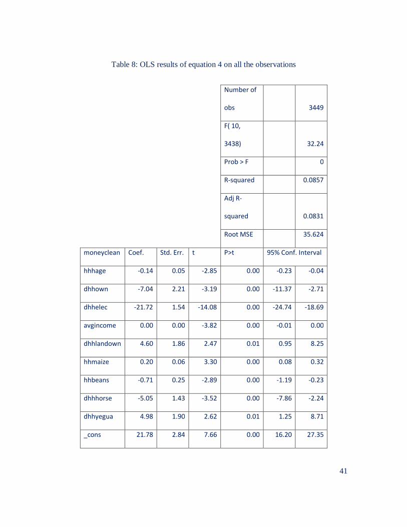
Using equation (4) we created 3 versions of our proxy for social distance. First

we ran equation (4) once for the full dataset and saved the residuals to use as our first

proxy for social distance and called it SOCDISALL, Table 8 presents the results of this

OLS regression. Second, we ran equation (4) 5 times, one per CR, and saved the

residuals as another proxy for social distance and called it SOCDISCR. Third, we ran

22

equation (4) 136 times and saved the residuals as SOCDIS136. We will use these 3

proxy measures for social distance in our estimation of the group formation equation (5).

We now estimate equation (5) using a logistic regression on our 3 measures of

social distance and for the individuals grouped by the result of the cluster analysis. Table

9 shows the results using SOCDISALL, Table 10 with SOCDISCR, and Table 11 with

SOCDIS136. Note that our 3 estimates of social distance are statistically significant and

positive. Also notice that we chose to report the odds ratio and not the beta estimate.

Although the results are the same, we prefer this presentation because we present the

impact on group membership by changing 1 unit of the independent variable,with

intuition comparable to the elasticity concept. Finally we will present our results

focusing on Table 11 that uses SOCDIS136. We do it for theoretical reasons: this

estimate is the one that reflects how much each individual decided to send to every other

individual participating in her meeting. As such this measure is “pure” from the point of

view of zero noise and avoiding the possibility that errors may be correlated within CR or

by CR. It is rewarding to report that this is the regression that offers the best fit—Pseudo

R2=0.7 compared against 0.6 for both alternative measures of social distance

SOCDISALL and SOCDISCR. The analysis in the following paragraphs of this section

refers to Table 11.

First: social distance matters for group formation. A key consideration for group

formation, in the context of bottom-up development programs, is to attempt to understand

the complex unobservable relationships that exist between people in communities. Free

from endogeneity issues, because our groups are based on cluster analysis, our results

23

show that the probability of membership increases when people are close. It is tempting

to run a regression of social distance on observable variables, however, this will be

misleading. Development practitioners have to make difficult decisions when designing

programs: either they prioritize strong social ties within the program, or they prioritize

program coverage. It may be the case, particularly in poor rural communities, that

practitioners cannot accomplish both objectives jointly because social distance “is” and is

inherited.

Second: it is easy to be misled by partial results. There are only 3 variables in

addition to social distance that point to increased inclusion: (i) households that have

horses; (ii) and (iii) households that grow beans and maize. Only the rich own a truck or

a car in rural western Honduras, however owning a horse reflects status and this may be

the reason why this dummy variable is so relevant for group formation. Additional

research may go into this arena, for this paper, however, we hypothesize that this finding

is consistent with our previous findings of the impact of education and income. A simple

status symbol, such as owning a horse, may reflect non-observable relevant

characteristics of individuals that merit attention by development practitioners. Beans

and maize are a puzzle because we concluded previously that maize and bean producers

were producing for self-consumption, and are over-represented in cluster group 2.

Because group 2 has less people belonging to CR than group 1 and therefore are less

educated and wealthy than group 1 people, we can only suggest that those maize and

bean producers in group 2 are members of the CR and are also big producers. The

message here to development practitioners is of caution about the observable

24

characteristics of potential participants because without a deep understanding of the

underlying foundations of group formation it is easy to be mislead by partial results.

Third: it is easy to be misled by partial results … again. Throughout this paper

we have repeatedly emphasized the role of household education and income/assets in

determining preferences and, implicitly, group formation. Look again at Table 11.

Gender, literacy, age, titling, and production diversification do not add much to group

formation. For this reason we emphasize again that unobservable variables are exactly

unobservable. We believe that proxy measures, such as those proposed by us in this

paper, have the potential to help us understand the complex human interactions when

deciding group membership.

Concluding remarks and policy recommendations.

We have attempted to solve the puzzle of group formation in the PRODERT

program. We show that differences in preferences for attributes of the program did not

explain group formation, an expected result given that these communities are relatively

homogenous. A closer look at the individual characteristics of participants, grouped by

CR membership and more by the results of the cluster analysis, shows significant

differences in their education, income, assets, and other factors. An even closer look at

individuals shows that they differentiate between members of the community, and they

send more money to the people they like more. Using this information we find that social

distance is central to explaining group formation in 5 communities in western Honduras.

25

We believe that this program has many lessons to teach in terms of rural and

regional development. We now turn to some final suggestions for development

practitioners.

What can a development practitioner learn from this paper?

First: it is not easy to find the balance between performance and coverage of

financial institutions. Effective programs require managing potential risks throughout the

project cycle. Excessive risk aversion on the part of CR may result in good performance

at the cost of low coverage. Beneficiaries self-selection may result in small strong groups

if the attributes of the program, the x, require strong commitments. Combining self-

selection and great commitment by beneficiaries may result in good programs that work

but that exhibit low coverage. Relaxing the demands imposed by program attributes may

increase coverage, but will also lower the cohesiveness of the group. Using what we

learned from analyzing PRODERT, then we suggest that if they want to increase

coverage then they may consider reviewing the lending terms offered by CR. Our results

show that the poorest of the poor do not like the idea of pledging collateral but recognize

the benefits of non-financial services. The introduction of lending terms that allow for

collateral-free loans at higher interest rates may be an interesting option for CR.

Conversely the inclusion of additional non-financial services may also induce people to

join the CR.

Second: eliciting preferences and proxy measures for social distance is not that

difficult. The identification of beneficiaries’ preferences for attributes of programs

provides relevant information that could be used during the design process of

26

development programs. Our field work included the execution of a survey with choice

experiments. It took about 20-30 minutes to execute the survey and choice experiments,

note that we were in the field, usually using a school for the meeting and that the

participants had on average 1.8 years of education. Eliciting information about social

distance is significantly more difficult and the results are less useful for the design of

programs. It takes great care and attention to detail to execute lab field experiments. We

spent twice as much time executing dictator and trust games as we spent executing the

survey. Moreover, this activity cannot be delegated to trained teams given the

complexity of the execution of this activity. However, social distance can be extremely

useful for the analysis of program results. In our paper we use social distance to analyze

group formation. In a different context, for example trying to determine the underlying

factors of failure/success of a program, social distance may provide key insights and add

a metric to unobservable characteristics of beneficiaries. In other words, our approach to

elicit a proxy for social distance may be used in different contexts and may provide a

measurable estimate being the alternative a subjective and non-testable approach to

talking about social distance.

27

References

Akerlof , G. 1997. “Social Distance and Social Decisions.” Econometrica, Vol.

65, No. 5; 1005-1027.

Ahlin, C. and R. M.Townsend, 2007. “Using Repayment Data to Test Across

Models of Joint Liability Lending.” The Economic Journal 117:517; F11-F51.

Banfield, E., 1958. The Moral Basis of a Backward Society Glencoe, Ill.: Free

Press & Chicago:Research Center in Economic Development and Cultural Change,

University of Chicago.

Cassar, A.; L. Crowley and B. Wydick, 2007. “The effect of social capital on

group loan repayment: evidence from field experiments.” The Economic Journal

117:517; F85-F106.

Dufhues, T.; F. Heidhues, and G. Buchenrieder, 2004. “Participatory Product

Design by Using Conjoint Analysis in the Rural Financial Market of Northern Vietnam.”

Asian Economic Journal 18 (1); 81–114.

Feder, G. and S. Savastano,2006. “The Role of Opinion Leaders in the Diffusion

of New Knowledge: The Case of Integrated Pest Management.” World Bank Policy

Research Working Paper 3916, World Bank, Washington, D.C.

Glaeser, E.L. G. Ponzetto and A. Shleifer, 2006. “Why Does Democracy Need

Education?” National Bureau of Economic Research, Working Paper 12128.

Gugerty, M.K. and M. Kremer, 2006. “Outside Funding and the Dynamics of

Participation in Community Associations.” BREAD Working Paper No. 128

28

Hermes, N. and R. Lensink, 2007. “The empirics of microfinance: what do we

know?.” The Economic Journal 117:517; F1-F10.

Hoffman E., K. McCabe and V. Smith, 1996. “Social Distance and Other-

Regarding Behavior in Dictator Games.” The American Economic Review, Vol. 86, No.

3; 653-660.

J ansen H., P. Siegel and J. Alwang 2005. Identifying the Drivers of Sustainable

Rural Growth and Poverty Reduction in Honduras. IFPRI DSGD Discussion Paper No.

19, IFPRI Washington DC.

Kuhfeld, W., 2005. Marketing Research Methods in SAS: Experimental Design,

Choice, Conjoint, and Graphical Techniques. SAS 9.1 Edition TS-722, SAS Institute,

Raleigh, NC.

Mansuri G. and V. Rao, 2004. “Community-Based and –Driven Development: A

Critical Review.” The World Bank Research Observer, 19(1);. 1-39.

Pichon, F. J. Alwang and P. Siegel 2006. Drivers of Sustainable Rural Growth

and Poverty Reduction in Central America: Guatemala Case Study. World Bank,

Washington DC.

Olson, M., 1965. The Logic of Collective Action. Cambridge: Harvard University

Press.

Pichon, F., P. Siegel, J. Alwang, K. Chomitz, C. Arce and J. Wadsworth 2006.

Nicaragua Drivers of Sustainable Rural Growth and Poverty Reduction in Central

America. Report No. 31193-NI. World Bank, Washington DC.

29

Siegel, P. and J. Alwang 1999. An Asset Based Approach to Social Risk

Management: A Conceptual Framework. Social Protection Discussion Series Paper No.

9926. World Bank, Washington DC.

Spoth, R., 1989. “Applying conjoint analysis of consumer preferences to the

development of utility-responsive health promotion programs.” Health Education

Research, Vol. 4, No. 4; 439-449.

Stiglitz J., 1990. “Peer Monitoring and Credit Markets.” World Bank Economic

Review; 351-366.

Walzer, Ml. 2002.“Equality and Civil Society” in Chambers, Simone and Will

Kylicka. Alternative Conceptions of Civil Society. Princeton: Princeton University Press.

Zeller, M. 1996. 1996. “Determinants of Repayment Performance in Credit

Groups: The Role of Program Design, Intragroup Risk Pooling, and Social Cohesion in

Madagascar.” FCND DISCUSSION PAPER NO. 13. International Food Policy

Research Institute, Washington, DC.

30

Table 1: Main results from our condition of sufficient social distance

Ceteris paribus: A

change from x to x’

that

Impact on social

distance

Explanation

Increases benefits None, but now

people that were far

will consider joining

if V(x) is now ≥0

For people that before were “too far” to

join with x, now join with increased

benefit related to x’

Decreases costs None, but now

people that were far

will consider joining

if V(x) is now ≥0

For people that before were “too far” to

join with x, now join with decreased cost

related to x’

31

Table 2: Choice experiments orthogonal arrayMEET NONFINCOLL SAVE

ALT 1 -1 -1 -1 1ALT 2 1 1 1 -1ALT 1 1 1 -1 1ALT 2 -1 -1 1 -1ALT 1 -1 1 1 1ALT 2 1 -1 -1 -1ALT 1 1 -1 1 1ALT 2 -1 1 -1 -1

SET 1

SET 2

SET 3

SET 4

32

Member Non-member G-1 G-2Count 72 64 87 49

Gender, 1=Female 1.78 1.78 1.79 1.76Head of HH literate, 1=Yes 1.26 1.38 1.15 1.61

Head of HH AGE 40.54 36.19 40.00 35.82HH number of members 6.26 5.17 6.24 4.88

HH literate members, number 3.68 2.63 3.91 1.90HH AGES (total years) 126.58 111.64 129.78 101.39

HH members years of ED (total years) 12.93 8.38 13.41 6.12HH CHILDREN under 8 years 1.67 1.50 1.59 1.59

HH LANDSIZE 5.44 3.58 6.03 1.97HH COFFEE production 18.13 16.92 23.76 6.55HH MAIZE production 10.58 11.14 9.03 14.06HH BEANS production 2.15 2.08 1.61 3.02

Table 3: Group characteristics, all averages except count

33

Table 4: Results of estimating parameters of conjoint analysis, conditional logit

FULL MEMBERS NON

MEMBERS

CLUSTER

14-1

CLUSTER

14-2

MEET

Estimate .21934 .24393 .19413 .24041 0.18981

Standard

error

.08893 .12360 .12984 .11024 0.15473

Chi-Square 6.0828 3.8947 2.2355 4.7561 1.5050

Pr>ChiSq .0137 .0484 .1349 .0292 0.2199

NONFIN

Estimate .44329 .52441 .35923 .40177 .54235

Standard

error

.08893 .12360 .12984 .11024 .15473

Chi-Square 24.8448 18.005 7.6553 13.2825 12.2868

Pr>ChiSq <.001 <.001 .0057 .0003 .0005

COLLATERAL

Estimate -.12608 -.07204 -.19413 .04857 -.45839

Standard

error

.08893 .12360 .12984 .11024 .15473

Chi-Square 2.0099 .3397 2.2355 .1941 8.7768

Pr>ChiSq .1563 .56 .1349 .6595 .0031

SAVE

Estimate .00593 .18547 -.19413 -.00228 .02247

Standard

error

.08893 .12360 .12984 .11024 .15473

Chi-Square .0045 2.2516 2.2355 .0004 .0211

34

Pr>ChiSq .9468 .1335 .1349 .983535 .8846

Note: Bold shaded indicates significant at 5%.

35

Table 5: PROBABILITY (%) OF CHOOSING AN ALTERNATIVE F ROM A

CHOICE SET

FULL MEMBERS NON

MEMBERS

CLUSTER

14-1

CLUSTER

14-2

CHOICE SET 1

2-2-2-1 37.037 37.500 36.509 33.336 43.750

1-1-1-2 62.963 62.500 63.491 66.664 56.250

CHOICE SET 2

1-1-2-1 68.883 73.611 63.491 64.367 77.083

2-2-1-2 31.117 26.389 36.509 35.633 22.917

CHOICE SET 3

2-1-1-1 52.593 59.722 44.444 55.172 47.917

1-2-2-2 47.407 40.278 55.556 44.828 52.083

CHOICE SET 4

1-2-1-1 41.482 45.833 36.509 47.126 31.250

2-1-2-2 58.518 54.167 63.491 52.874 68.750

36

Table 6: Results of estimating parameters of conjoint analysis, mixed logit

FULL MEMBERS NON

MEMBERS

CLUSTER

14-1

CLUSTER

14-2

MEET

Estimate -.26940 -.01839 -.38022 -0.28017 -0.1985

Standard error .21952 .35441 .29837 0.35902 0.33615

Chi-Square 1.5061 .0027 1.6239 0.609 0.3487

Pr>ChiSq .2197 .9586 .2026 0.4352 0.5549

NONFIN

Estimate .23605 .26517 .30831 0.18727 0.02454

Standard error .21952 .35441 .29837 0.35902 0.33615

Chi-Square 1.1563 .5598 1.0677 0.2721 0.0053

Pr>ChiSq .2822 .4543 .3015 0.6019 0.9418

COLLATERAL

Estimate -.64641 -.84627 -.5406 -0.28828 -0.71977

Standard error .21952 .35441 .29837 0.35902 0.33615

Chi-Square 8.6712 5.7019 3.2827 0.6448 4.5848

Pr>ChiSq .0032 .0169 .07 0.422 0.0323

SAVE

Estimate -.00576 .20784 -.06425 0.03741 0.17835

Standard error .21952 .35441 .29837 0.35902 0.33615

Chi-Square .0007 .3439 .0464 0.0109 0.2815

Pr>ChiSq .9791 .5576 .8395 0.917 0.5957

37

PCTLIT*MEET

Estimate .87390 .37678 1.18744 0.73204 2.04359

Standard error .38455 .61582 .52678 0.55708 0.77771

Chi-Square 5.1644 .3743 5.0811 1.7268 6.9048

Pr>ChiSq .0231 .5406 .0242 0.1888 0.0086

PCTLIT*NONFIN

Estimate .39327 .40623 .21736 0.34928 1.05867

Standard error .38455 .61582 .52678 0.55708 0.77771

Chi-Square 1.0458 .4352 .1703 0.3931 1.853

Pr>ChiSq .3065 .5095 .6799 0.5307 0.1734

PCTLIT*COLL

Estimate 1.05578 1.19363 .96444 0.61779 0.85293

Standard error .38455 .61582 .52678 0.55708 0.77771

Chi-Square 7.5378 3.7570 3.3518 1.2298 1.2028

Pr>ChiSq .0060 .0526 .0671 0.2674 0.2728

PCTLIT*SAVE

Estimate .21816 -.05572 .14396 0.0725 1.1321

Standard error .38455 .61582 .52678 0.55708 0.77771

Chi-Square .3218 .0082 .0747 0.0169 2.119

Pr>ChiSq .5705 .9279 .7846 0.8965 0.1455

AVGINCOME*MEET

Estimate .0000447 .0000101 .0001371 0.000095 -0.00069

Standard error .0001368 .0002334 .0002157 0.000143 0.000505

38

Chi-Square .1068 .0019 .4037 0.4398 1.8417

Pr>ChiSq .7438 .9654 .5252 0.5072 0.1747

AVGINCOME

*NONFIN

Estimate .0000555 .0000608 .0001118 3.64E-05 0.000386

Standard error .0001368 .0002334 .0002157 0.000143 0.000505

Chi-Square .1648 .0678 .2687 0.0645 0.5841

Pr>ChiSq .6848 .7946 .6042 0.7996 0.4447

AVGINCOME *COLL

Estimate -.0000834 .0001719 -.0002968 -6.9E-05 -0.00036

Standard error .0001368 .0002334 .0002157 0.000143 0.000505

Chi-Square .3715 .542 1.8926 0.233 0.5187

Pr>ChiSq .5422 .4616 .1689 0.6293 0.4714

AVGINCOME *SAVE

Estimate -.0001892 -.0000419 -.0002307 -0.00015 -0.00088

Standard error .0001368 .0002334 .0002157 0.000143 0.000505

Chi-Square 1.9135 .0322 1.1436 1.1375 3.0302

Pr>ChiSq .1666 .8576 .2849 0.2862 0.0817

HHLANDSIZE*MEET

Estimate -.0001376 .00929 -0.02824 0.000772 -0.0055

Standard error .0089 .01258 0.02509 0.00898 0.05188

Chi-Square .0002 .5448 1.267 0.0074 0.0112

Pr>ChiSq .9877 .4605 0.2603 0.9315 0.9156

39

HHLANDSIZE

*NONFIN

Estimate -.00498 .00106 -0.0327 -0.00353 0.00652

Standard error .0089 .01258 0.02509 0.00898 0.05188

Chi-Square .3126 .0071 1.6986 0.1543 0.0158

Pr>ChiSq .5761 .9328 0.1925 0.6944 0.8999

HHLANDSIZE

*COLL

Estimate .00276 .0000435 0.0187 0.000777 0.03268

Standard error .0089 .01258 0.02509 0.00898 0.05188

Chi-Square .0958 .0071 0.5557 0.0075 0.3968

Pr>ChiSq .7569 .9328 0.456 0.9311 0.5287

HHLANDSIZE *SAVE

Estimate -.0000311 .00555 -0.02365 0.00227 -0.07061

Standard error .0089 .01258 0.02509 0.00898 0.05188

Chi-Square 0 .1946 0.8888 0.0641 1.8523

Pr>ChiSq .9972 .6591 0.3458 0.8001 0.1735

Note: Bold shaded indicates significant at 5%.

40

Table 7: PROBABILITY (%) OF CHOOSING AN ALTERNATIVE F ROM A CHOICE SET

FULL MEMBERS NON MEMBERS

CLUSTER 14-1

CLUSTER 14-2

CHOICE SET 1

2-2-2-1 45.542 33.587 42.525 43.706 37.296

1-1-1-2 54.458 66.413 57.475 56.294 62.704

CHOICE SET 2

1-1-2-1 67.847 70.663 61.569 60.986 86.093

2-2-1-2 32.153 29.337 38.431 39.014 13.907

CHOICE SET 3

2-1-1-1 51.435 62.652 48.152 55.832 51.394

1-2-2-2 48.565 37.348 51.848 44.168 48.606

CHOICE SET 4

1-2-1-1 35.983 45.239 33.533 41.278 29.145

2-1-2-2 64.017 54.761 66.467 58.722 70.855

41

Table 8: OLS results of equation 4 on all the observations

Number of

obs 3449

F( 10,

3438) 32.24

Prob > F 0

R-squared 0.0857

Adj R-

squared 0.0831

Root MSE 35.624

moneyclean Coef. Std. Err. t P>t 95% Conf. Interval

hhhage -0.14 0.05 -2.85 0.00 -0.23 -0.04

dhhown -7.04 2.21 -3.19 0.00 -11.37 -2.71

dhhelec -21.72 1.54 -14.08 0.00 -24.74 -18.69

avgincome 0.00 0.00 -3.82 0.00 -0.01 0.00

dhhlandown 4.60 1.86 2.47 0.01 0.95 8.25

hhmaize 0.20 0.06 3.30 0.00 0.08 0.32

hhbeans -0.71 0.25 -2.89 0.00 -1.19 -0.23

dhhhorse -5.05 1.43 -3.52 0.00 -7.86 -2.24

dhhyegua 4.98 1.90 2.62 0.01 1.25 8.71

_cons 21.78 2.84 7.66 0.00 16.20 27.35

42

Table 9: Logistic results of equation 5 on all SOCDISALL

Logistic regression Number of obs 1896

LR chi2(11) 1253.09

Prob > chi2 0

Log likelihood = -423.98549 Pseudo R2 0.5964

CSen Odds Ratio Std. Err. z P>z [95% Conf. Interval

socdisALL 1.02 0.01 2.26 0.02 1.00 1.05

dgender 0.31 0.08 -4.70 0.00 0.19 0.51

dhhhlit 0.01 0.00 -15.84 0.00 0.00 0.01

hhmem 0.53 0.03 -10.53 0.00 0.48 0.60

dhhtitle 0.07 0.02 -11.50 0.00 0.05 0.11

hhcoffee 0.92 0.01 -8.61 0.00 0.90 0.94

hhmaize 1.06 0.01 5.66 0.00 1.04 1.08

hhbeans 1.84 0.09 11.95 0.00 1.67 2.04

ddiversified 0.43 0.11 -3.33 0.00 0.26 0.70

dhhmulas 0.03 0.02 -7.30 0.00 0.01 0.08

dhhyegua 0.15 0.05 -5.96 0.00 0.08 0.28

43

Table 10: Logistic results of equation 5 on all SOCDISCR

Logistic regression Number of obs 1896

LR chi2(11) 1277.56

Prob > chi2 0

Log likelihood = -411.7489 Pseudo R2 0.6081

CSen

Odds

Ratio Std. Err. z P>z

[95% Conf.

Interval]

socdisCR 1.19 0.04 5.30 0.00 1.11 1.27

dgender 0.42 0.10 -3.72 0.00 0.26 0.66

dhhhlit 0.01 0.00 -16.28 0.00 0.00 0.01

hhmem 0.53 0.03 -10.71 0.00 0.47 0.59

dhhtitle 0.07 0.02 -11.57 0.00 0.04 0.11

hhcoffee 0.92 0.01 -8.64 0.00 0.90 0.94

hhmaize 1.06 0.01 5.23 0.00 1.03 1.08

hhbeans 1.81 0.09 11.74 0.00 1.64 1.99

ddiversified 0.44 0.11 -3.24 0.00 0.26 0.72

dhhmulas 0.03 0.01 -7.63 0.00 0.01 0.07

dhhyegua 0.15 0.05 -5.90 0.00 0.08 0.28

44

Table 11: Logistic results of equation 5 on all SOCDIS136

Logistic regression Number of obs 1896

LR chi2(13) 1464.09

Prob > chi2 0

Log likelihood = -318.48424 Pseudo R2 0.6968

CSen

Odds

Ratio Std. Err. z P>z

[95% Conf.

Interval]

socdis136 1.02 0.01 2.73 0.01 1.01 1.04

dgender 0.28 0.07 -4.84 0.00 0.16 0.46

dhhhlit 0.00 0.00 -12.56 0.00 0.00 0.01

hhmem 0.45 0.04 -9.36 0.00 0.38 0.53

hhavged 0.21 0.03 -10.95 0.00 0.16 0.27

dhhhorse 3.53 1.30 3.44 0.00 1.72 7.25

dhhtitle 0.09 0.02 -9.01 0.00 0.06 0.16

hhcoffee 0.86 0.01 -8.97 0.00 0.83 0.89

hhmaize 1.09 0.01 6.73 0.00 1.07 1.12

hhbeans 2.26 0.16 11.15 0.00 1.96 2.60

ddiversified 0.18 0.06 -4.88 0.00 0.09 0.36

dhhmulas 0.01 0.01 -6.56 0.00 0.00 0.04

dhhyegua 0.08 0.04 -5.07 0.00 0.03 0.21

45

Figure 1: Choice set 1 of conjoint questions

46

Annex I—Dictator Game protocol

The traditional dictator game

To capture measures of altruism we employ the commonly play dictator game,

which is a simple decision game void of strategic interaction. In the decision game one

person (call her the dictator) receives an endowment M and is faced with the decision of

how to split the endowment between herself and a second person. The money ‘sent’ to

the second person is sometimes multiplied by some factor greater than one. For example,

in our experiment we multiply the amount the dictator sends to the second person by a

factor of two. The dictator’s identity is usually not observed by the second person so that

the amount the dictator sends to the second person is considered a measure of altruism. If

the dictator does not know the identity of the second person then we consider the amount

sent by the dictator to the second person as a measure of generic altruism.

However, one may devise the experiment so that the dictator knows the identity of

the second person, while at the same time preserving the anonymity of the dictator.

When an anonymous dictator knows the identity of the second person, we consider the

amount sent by the dictator to be a measure of directed altruism. If we assume social

preferences over the second person’s monetary payout (rather than the second person’s

utility) then directed altruism may be considered a measure of social distance. This

interpretation relies on the intuitive notion that the closer I am to you socially, then the

more weight I put on your monetary payout in my utility function. Having said that, if

social preferences are over others’ utilities then directed altruism is a combination of

social distance and the dictator’s distributional preferences. That is, assuming social

47

preferences over others’ utilities rather than others’ monetary payouts recognizes the fact

that I may be socially closer to my wealthy brother than a homeless person, but I may, in

fact, give more to a homeless person than my wealthy brother.

Description of dictator game protocol

Detailed oral instructions were provided at the beginning of the experiment

session. We also developed several examples of how to play the game. We explained

the directed dictator game first (the dictator game in which the identity of the second

person was revealed to the dictator). Once everyone understood the game we randomly

assigned each person to a seat so that a large circle was formed. In order to maintain the

privacy of decision-making throughout the experiment, each person was given a privacy

box that sat on their lap. Next we picked a random person’s name from the circle and

asked them to go to the center of the circle. Those participants remaining in their seats

each played the role of the dictator in the dictator game while the person in the center

played the role of the “second person” in the dictator game. Everyone except the person

in the center of the circle was given an empty envelope and a ticket (see ticket below)

with their personal identification code on the back of the ticket. We asked each person to

mark an ‘X’ in the row corresponding to their own desires for distributing money

between them and the second person in the center of the room. Once each person made

their decision, they were instructed to put their ticket in the envelope and place the

envelope on top of their privacy box. We explicitly reminded them to mark an ‘X’ in

only one row on the ticket. Next someone collected the envelopes and mixed the

envelopes in random order. The envelopes were put in a bag and mixed again, and then

48

the “second person” in the center of the room randomly picked one of the envelopes.

This randomly selected envelope went into the center person’s yellow compensation

folder. The person in the center was reminded that at the end of the day that their yellow

compensation folder would have six such envelopes. Each person would randomly pick

one of the six envelopes from their yellow compensation envelope and this would be their

compensation for the day. Next, the person in the center of the room returned to their

seat and a new person from the circle was randomly called to the center. We repeated

this process until everyone had passed to the center of the circle. In this way we were

able to obtain a full mapping of directed altruism measures between all participants in the

experiment. That is, for each individual i in the experiment we were able to obtain a

measure of directed altruism towards each participant j (j not equal to i) in the

experiment.

After this directed dictator game was completed we had the participants play a

generic dictator game. In this version no one passed to the center of the circle. This

signified that as dictator they would not know the identity of the second person in the

dictator game (the person with whom they were splitting the money). That is, each

person would make a decision and then we would randomly assign the envelopes to a

second person, and these envelopes would go in each second person’s yellow [prize]

folder. In this way we were able to obtain a measure of generic altruism.

Next we played two final rounds of generic dictator games, each with a slight

variation. In one dictator game we informed the participants that they would play a

generic dictator game where they knew the second person was a member of the CR. That

49

is, after everyone made their decision as dictator, we mixed up the envelopes, put them in

a bag and then had each participant who was a member of the caja rural randomly select

an envelope. When they selected their envelope they put it in their yellow compensation

folder. In this way we were able to obtain measures of generic altruism towards members

of the CR.

In the final generic dictator game we informed the participants that they would

play a generic dictator game where they knew the second person was a not a member of

the CR. That is, after everyone made their decision as dictator, we mixed up the

envelopes, put them in a bag and then had each participant who was not a member of the

caja rural randomly select an envelope. When they selected their envelope they put it in

their yellow compensation folder. In this way we were able to obtain measures of generic

altruism towards non-members of the caja rural.

To summarize, the experiments we used allowed us to collect four measures of

altruism for each individual: 1) a measure of directed altruism towards a specific

individual; 2) a measure of generic altruism towards community members; 3) a measure

of generic altruism towards community members in the CR; and 4) a measure of generic

altruism towards community members not in the CR.

You Other Person Mark one‘X’

50 0

45 10

40 20

35 30

50

30 40

25 50

20 60

15 70

10 80

5 90

0 100

1 This is the only endnote in this paper and is intended to reflect our deep appreciation for

Warren Kuhfeld of SAS Institute. During the design process of the conjoint choice sets

we ran into some issues: we wanted a small yet main effects design that would minimize

the number of choice sets and alternatives within sets. Being stuck, we sent an email to

Dr. Kuhfeld, someone that we have not met in person nor, until that point, had we

exchanged any correspondence. He responded with a complete answer within minutes,

including suggestions to improve the design. Such disinterested commitment to science

is remarkable and we use this unique footnote to thank him for his support. We hope

students and practitioners read papers thoroughly, footnotes included. All errors in the

paper are, as they should be, ours.