Explanation-Based Learning:

A Survey of Programs and Perspectives

Thomas Ellman

May 1987

CUCS-266-87

Table of Contents 1 Introduction

1.1 An Intuitive Example of EBl 1.2 Overview of this Paper

2 Background of EBl 2.1 Why is EBl Necessary? 2.2 The History of EBl 2.3 Relation to other Machine learning Research

3 Selected Examples of Explanation-Based learning 3.1 Introduction 3.2 EBl = Justified Generalization

3.2.1 The GENESIS System (DeJong and Mooney) 3.2.2 The lEX-II System (Mitchell and Utgoff) 3.2.3 Similar Work

3.3 EBl = Chunking 3.3.1 The SOAR System (Rosenbloom, laird and Newell) 3.3.2 The STRIPS System (Fikes, Hart & Nilsson) 3.3.3 Similar Work

3.4 EBl = Operationalization 3.4.1 Mostow's FOO and BAR Programs 3.4.2 Keller's lEXCOP System 3.4.3 Similar Work

3.5 EBl = Justified Analogy 3.5.1 Winston's ANALOGY Program 3.5.2 Carbonell's Derivational Analogy Method 3.5.3 Analogy versus Generalization 3.5.4 Similar Work

3.6 Additional Related EBl Research 4 Formalizations of Explanation-Based learning

4.1 Mitchell's EBG Formalism 4.2 Other Formalizations

5 An Evaluation of EBl 6 Future EBl Research

6.1 EBl and Theory Reformulation 6.2 EBl and Theory Revision 6.3 EBl and SBl

7 Summary 8 Acknowledgement

I. Glossary of Selected Terms

2 2 4 5 5 6 8 9 9 9 9

17 24 25 25 32 37 37 38 41 44 44 45 48 50 51 52 53 53 55 56 58 58 62 66 68 68 69

II

List of Figures Figure 1: A Training Example from Hearts Figure 2: A New Hearts Example Covered by the General Rule Figure 3: Relation between Views of EBl Figure 4: A Story that GENESIS Reads and Generalizes Figure 5: A Causally Complete Explanation of the Kidnapping Figure 6: Generalization Procedure used by GENESIS Figure 7: EGGS Procedure Figure 8: The Generalized Kidnapping Network Figure 9: Examples of Operators Used in lEX-I and lEX-II Figure 10: Partial Search Tree labeled by Critic Module Figure 11: Rules Defining the POSINST Predicate in lEX-II Figure 12: Organization of the lEX-II Generalizer Figure 13: EBl Procedure Used in LEX-II Figure 14: Proof Tree Built by lEX-II Figure 15: Hierarchy of Goal Contexts in SOAR Figure 16: Initial and Goal States for 8-Puzzle Figure 17: Trace of SOAR Execution on 8-Puzzle Figure 18: Chunking Procedure In SOAR Figure 19: Abstract Operator Created by SOAR Figure 20: STRIPS' Initial World Model FIgure 21: Examples of STRIPS Operators Figure 22: Example of a Triangle Table Figure 23: Definition of Triangle Table Figure 24: STRIPS Generalization Procedure Figure 25: Generalized Triangle Table Figure 26: Problem Transformation Rules Figure 27: Concept Definitions Figure 28: Rules Defining the POSINST Predicate In lEXCOP Figure 29: Translated Concept Description Figure 30: Transformation Rules In lEXCOP Figure 31: Functional Definition of a Cup Figure 32: Example of a Cup Figure 33: Final Version of Example Network Figure 34: Rule Extracted From Network Figure 35: The EBG Problem Figure 36: Four Interpretations of EBG Figure 37: Types of Imperfect Theories

3 4

10 10 12 13 15 16 17 18 19 19 20 20 26 27 28 30 31 33 33 34 34 35 36 39 39 42 42 43 45 46 47 47 54 55 63

1

Explanation-Based Learning:

A Survey of Programs and Perspectives

Thomas Ellman Columbia University

Department of Computer Science New York, New York 10027

(212) 280-8182 Ellman@CS.COlUMBIA.EDU

Abstract

"Explanation-Based learning" (EBl) is a technique by which an intelligent system can learn by observing examples. EBl systems are characterized by the ability to create justified generalizations from single training instances. They are also distinguished by their reliance on background knowledge of the domain under study. Although EBl is usually viewed as a method for performing generalization, it can be viewed in other ways as well. In particular, EBl can be seen as a method that performs four different learning tasks: generalization, chunking, operationalization and analogy.

This paper provides a general introduction to the field of explanation-based learning. It places considerable emphasis on showing how EBl combines the four learning tasks mentioned above. The paper begins by presenting an intuitive example of the EBl technique. It subsequently places EBl in its historical context and describes the relation between EBl and other areas of machine learning. The major part of this paper is a survey of selected EBl programs. The programs have been chosen to show how EBl manifests each of the four learning tasks. Attempts to formalize the EBl technique are also briefly discussed. The paper concludes by discussing the limitations of EBl and the major open questions in the field.

Categories and Subject Descriptors: 1.2.6 [Artificial Intelligence]: learning­concept learning; induction; analogies; knowledge acquisition

General Terms: Experimentation

Additional Key Words and Phrases: machine learning, concept acquisition, explanation-based learning, generalization, chunking, operationalization, analogy, goal-regression, similarity-based learning.

2

1 Introduction

Research in the field of machine learning has identified two contrasting approaches to the

problem of learning from examples. The traditional method is sometimes known as

similarity-based learning (SBl).1This technique involves examining multiple examples of a

concept in order to determine the features they have in common. Researchers using this

"empiricalM approach have assumed that an intelligent system can learn from examples without

having much prior knowledge of the domain under study. Some well known examples of

similarity-based learning are [Winston 72; Michalski 80; Lebowitz 83] among others. This

research is surveyed in [Angluin and Smith 83; Cohen and Feigenbaum 82; Michalski 83;

Michalski et al. 83; Mitchell 82a]. An alternative technique known as explanation-based

learning (EBl) has been developed more recently. This Manalytical" approach attempts to

formulate a generalization after observing only a single example. In contrast to SBl, the EBl

method requires that a learning system be provided with a great deal of domain knowledge at

the outset. Some examples of the EBl technique are [Mitchell 83a; DeJong 86; Carbonell 86;

Mostow 83a] among others described below.

1.1 An Intuitive Example of EBl

EBl is based on the hypothesis that an intelligent system can learn a general concept

after observing only a single example. In order to illustrate how this can be done, consider the

following example taken from the card game MheartsM.2 Imagine a student who is learning to play

the game of hearts by looking over the shoulder of a teacher who is actually playing the game.

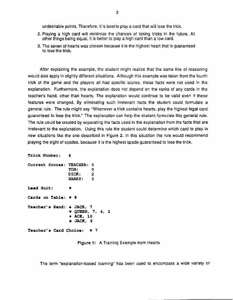
The teacher is faced with the situation described in Figure 1. The leader of the current trick has

just played the eight of hearts. According to the rules, the teacher must play one of his hearts.

He can choose either the queen, the seven, the four or the two of hearts. It turns out that the

teacher chooses to play the seven of hearts. The student might explain the teacher's choice

with the following line of reasoning.

1. This trick contains hearts. The winner of the trick will accumulate some

1 A glossary of selected terms may be found in Appendix I. Each term in the glossary will be written in boldface the first time it appears in this paper.

2Hearts is normally played with four players. Each player is dealt thirteen cards. At the start of the game, one player is designated to be the -'eader". The game is divided into thirteen successive tricks. At the start of each trick, the leader plays a card. Then the other players play cards in order going clockwise around the circle. Each player must playa card matching the suit of the card played by the leader, if he has such a card in his hand. Otherwise, he may play any card. The player who plays the highest card in the same suit as the leader's card will take the trick and become the leader for the next trick. Each player receives one point for every card in the suit of hearts contained in a trick that he takes. In the simplest version of the game, the objective is to minimize the number of points in one·s score. Other versions are more complicated. Complete rules are found in [Gibson 74].

3

undesirable points. Therefore, it is best to playa card that will lose the trick.

2. Playing a high card will minimize the chances of taking tricks in the future. All other things being equal, it is better to playa high card than a low card.

3. The seven of hearts was chosen because it is the highest heart that is guaranteed to lose the trick.

After explaining the example, the student might realize that the same line of reasoning

would also apply in slightly different situations. Although this example was taken from the fourth

trick of the game and the players all had specific scores, these facts were not used in the

explanation. Furthermore, the explanation does not depend on the ranks of any cards in the

teacher's hand, other than hearts. The explanation would continue to be valid even if these

features were changed. By eliminating such irrelevant facts the student could formulate a

general rule. The rule might say "Whenever a trick contains hearts, play the highest legal card

guaranteed to lose the trick." The explanation can help the student formulate this general rule.

The rule could be created by separating the facts used in the explanation from the facts that are

irrelevant to the explanation. Using this rule the student could determine which card to play in

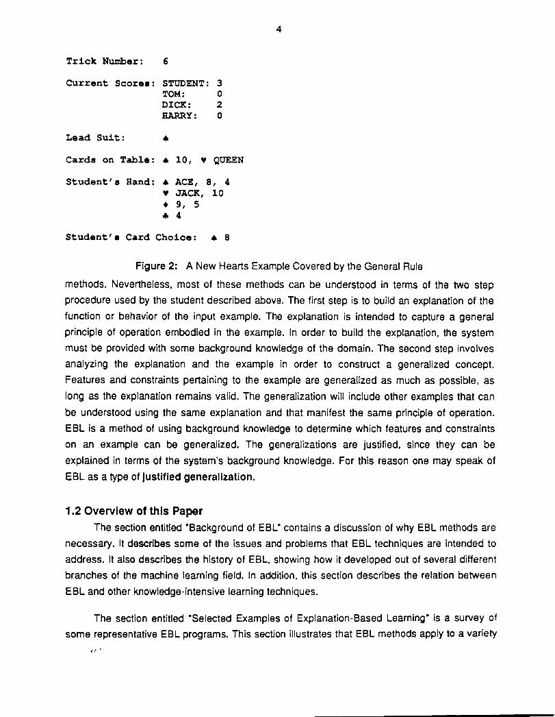
new situations like the one described in Figure 2. In this situation the rule would recommend

playing the eight of spades, because it is the highest spade guaranteed to lose the trick.

Trick Number: 4

Current Score.: TEACHER: 0 TOM: 0 DICX: 2 HARRY: 0

Lead Suit: • Card. on Table: • 8

Teacher'. Band: • JACK, 7 • QUEEN, 7, 4, 2 • ACll, 10 ... JACK, 9

Teacher'. Card Choice: • 7

Figure 1: A Training Example from Hearts

The term -explanation-based learning- has been used to encompass a wide variety of

4

Trick Number: 6

CUrrent Score.: STUDENT: 3 TOM: 0 DICK: 2 BARRY: 0

Lead Suit: ""

Cards on Table: "" 10, • QUEEN

Student's Band: "" ACE, 8, 4 • JACK, 10 • 9, 5

"" 4

Student'. Card Choice: "" 8

Figure 2: A New Hearts Example Covered by the General Rule

methods. Nevertheless, most of these methods can be understood in terms of the two step

procedure used by the student described above. The first step is to build an explanation of the

function or behavior of the input example. The explanation is intended to capture a general

principle of operation embodied in the example. In order to build the explanation, the system

must be provided with some background knowledge of the domain. The second step involves

analyzing the explanation and the example in order to construct a generalized concept.

Features and constraints pertaining to the example are generalized as much as possible, as

long as the explanation remains valid. The generalization will include other examples that can

be understood using the same explanation and that manifest the same principle of operation.

EBl is a method of using background knowledge to determine which features and constraints

on an example can be generalized. The generalizations are justified, since they can be

explained in terms of the system's background knowledge. For this reason one may speak of

EBl as a type of Justified generalization.

1.2 Overview of this Paper The section entitled "Background of EBl" contains a discussion of why EBl methods are

necessary. It describes some of the issues and problems that EBl techniques are intended to

address. It also describes the history of EBl, showing how it developed out of several different

branches of the machine learning field. In addition, this section describes the relation between

EBl and other knowledge-intensive learning techniques.

The section entitled ·Selected Examples of Explanation-Based learning" is a survey of

some representative EBl programs. This section illustrates that EBl methods apply to a variety 4,.' •

5

of learning tasks including generalization, chunking, operationalization and analogical

reasoning. The section is divided into four parts corresponding to these four learning tasks. For

each type of task, several EBl programs that perform the task are described. This section also

shows that differences between the four categories of EBl programs are largely a matter of

interpretation. The operation of most EBl programs can be interpreted in terms of any of the

four learning tasks.

The section entitled "Formalizations of Explanation-Based learning" describes attempts

to precisely define the methods of EBl, the requirements for building EBl systems and the

types of learning tasks that EBl can handle. The formalization also serves to clarify the relation

between the four categories of EBl systems. The section entitled "An Evaluation of EBl"

addresses the question of whether EBl systems can really learn anything they do not already

know. The final section, entitled "Future EBl Research", contains a discussion of major open

problems in the EBl field and some ongoing attempts to resolve them.

2 Background of EBl

2.1 Why Is EBl Necessary? The methods of explanation-based learning have been developed to address several

different issues in the field of machine learning. One issue involves human learning abilities.

Some EBl research has been motivated by the observation that people are often able to learn a

general rule or concept after observing a single instance of the concept. It is worth noting that

the EBl literature does not cite any experimental evidence that people can learn from single

examples. Such an experiment would be a worthwhile contribution. Nevertheless, textbooks

provide some evidence for this type of learning. For instance, a textbook on logic circuits

presents an example of a three bit shift register and then asks the student to design a four bit

shift register as an exercise [Mano 76], (page 7S). In order to solve the problem, the student

would presumably generalize or transform the single example of a three bit shift register. The

techniques of similarity-based learning are not suitable for learning from a single example. SBl

normally involves examining two or more instances of a concept. EBl is specifically designed

for generalizing from a single example and is therefore able to model a type of human learning

outside the scope of SBL.

EBl methods also address a more theoretical issue. EBl may be viewed as an attempt to

solve the problem of inductive bias. As described by Mitchell in [Mitchell SO], every system that

learns from examples requires some sort of bias. Mitchell defines bias to be "any basis for

choosing one generalization over another, other than strict consistency with the observed

6

training instances· [Mitchell 80]. (page 1). A system lacking inductive bias would not be capable

of making predictions beyond the training examples it has already seen. Typical types of bias

include using a restricted vocabulary in the generalization language [Utgoff 86] and restricting

the form of concept descriptions to conjunctive expressions [Vere 75]. EBL may be viewed as

an attempt to use "background knowledge" or a "domain model· as a type of bias. The EBL

method is biased toward making generalizations that can be justified by explaining them in

terms of the domain model. EBL programs usually represent domain knowledge in a declarative

style. EBL may therefore be said to utilize a declarative bias representation.

Several advantages result from representing bias in terms of a declarative domain model.

To begin with. a declarative bias can be interpreted in terms of direct statements about the

domain. For this reason. the bias is subject to evaluation by human experts even· before it is

used to process training examples. By comparison. a bias such as a restricted vocabulary is not

immediately interpretable as a statement about the domain [Dietterich 86]. It therefore cannot

be easily evaluated except by testing its consistency with the training examples [Russell and

Grosof 87]. A declarative bias also offers advantages of domain independence. As observed in

[Dietterich and Michalski 81]. greater domain independence is achieved if the bias is contained

in a separate module. The declarative domain models used by EBL systems are usually kept

separate and can be easily mOdified. Traditional types of bias. such as the two cited above. are

normally built in to the representation and procedures used by the learning system. For this

reason they are not easily modifiable. A declarative bias representation also helps to integrate

diverse sources of background knowledge into the learning process [Russell and Grosof 87].

2.2 The History of EBl

Explanation-based learning has only recently emerged as a recognizable area of study.

Consequently, most early EBL research was undertaken by investigators who were not working

on "explanation-based learning- per se. EBL may be viewed as a convergence of several

distinct lines of research within machine learning. In particular. EBL has developed out of

efforts to address each of the following problems: • Justified Generalization: A logically sound procedure for generalizing from

examples. Given some initial background knowledge B and a set of training examples T, justified generalization finds a concept C that includes all the positive examples and excludes all the negative examples. The learned concept C must be a logical consequence of the background knowledge B and the training example set T [Russell 86] .

• Chunklng: In the context of explanation-based learning, chunking is a process of compiling a linear or tree-structured sequence of operators into a single operator. The Single operator has the same effect as the entire original sequence [Rosenbloom and Newell 86].

7

• Operatlonallzatlon: A process of translating a non-operational expression into an operational form. The initial non-operational expression may be a set of instructions or a concept. Concepts and instructions are considered to be operational with respect to an agent if they are expressed in terms of actions and data available to the agent [Mostow 83a] .

• Justified Analogy: A logically sound procedure for reasoning by analogy. Given some initial background knowledge B, an analogue example A and a target example B, find a feature F such that F(A) and infer that F(B). The conclusion F(B) must be a logical consequence of F(A) the background knowledge B [Davies and Russell 86].

Two of the first investigators to develop EBl methods were DeJong and Mitchell.

DeJong's first paper in the EBl genre was [DeJong 81], which outlines a method of using

explanations to learn procedural schemata from natural language input. DeJong viewed his

approach as an attempt to model "insight learning" that involves "grasping a principle" embodied

in an example [DeJong 81], (page 67). Mitchell's first EBl program was the lEX-II system

developed jointly with Utgoff. This system involved a method of learning search control

heuristics by analyzing sequences of operators [Utgoff 82]. Mitchell's overall approach to EBl

was first outlined in his Computers and Thought paper [Mitchell 83a]. In this paper, he

suggested that a learning system be given "declarative knowledge of its learning goal" [Mitchell

83a], (page 1145). Such knowledge would enable a system to make "justifiable" generalizations

and would be more powerful than purely "empirical" or "syntactic" methods.

At the same time that Mitchell and DeJong were developing EBl methods of

generalization, Carbonell introduced his method of derivational analogy [Carbonell 83a].

Carbonell's method uses derivations as a guide to analogical reasoning in a manner similar to

the way in which EBl uses explanations to guide generalization. Winston was another one of

the first investigators to use EBl methods in the context of reasoning by analogy [Winston et al.

83]. The EBl methods used by Carbonell and Winston are both similar to Gentner's "structure­

mapping" theory of analogy [Gentner 83]. They also bear a resemblance Banerji and Ernst's

method of using homomorphisms to implement a type of analogical reasoning [Banerji and

Ernst 72].

One of the first operationalizing systems was Mostow's FOO program for operationalizing

advice [Mostow 81]. Keller's concept operationalization technique [Keller 83] was another early

program that performs operationalization. The techniques used by Keller and Mostow bear a

strong resemblance Balzer's method of "transformational implementation" [Balzer et aI. 76]. A

general approach to the problem of operationalizing advice is discussed in [Hayes-Roth and

Mostow 81]. This line of research can be ultimately traced back to McCarthy's suggestion for an

advice taking program [McCarthy 68]. All of these systems may be seen as implementing a type

8

of "learning by being told" [Cohen and Feigenbaum 82].

The STRIPS system [Fikes et a\. 72] was one of the first programs to perform chunking.

Although STRIPS uses explanation-based methods for generalizing robot plans, it was not

viewed as an EBL system by its authors, since it was built well before EBL became a

recognized field of study. The idea of combining individual operators into macros goes back to

Amarel's paper on representations for the "missionaries and cannibals" problem [Amarel 68].

The idea of chunking can ultimately be traced back to Miller's psychological studies [Miller 56].

Schank and Silver may also be credited with contributions to early EBL research. Schank

has discussed a learning process that involves finding explanations for observed anomalies, or

prediction failures [Schank 82]. Silver has developed a method called "precondition-analysis"

for learning search control strategies [Silver 86].

2.3 Relation to other Machine Learning Research EBL is characterized by the fact that it makes use of extensive background knowledge to

guide the learning process. A number of researchers outside the area of EBL have also used

such knowledge-intensive approaches to machine learning. Some early examples include

Lenat's AM program [Lenat 82], Sussman's HACKER program [Sussman 75] and Soloway's

program for learning rules of competitive games [Soloway 77]. These systems are difficult to

compare since they use diverse program architectures. Their background knowledge is

embedded in specialized, domain dependent heuristics, such as Lenat's heuristics for creating

and evaluating concepts and Sussman's knowledge base of bugs and patches. Additional

programs using knowledge-intensive learning techniques include [Buchanan and Mitchell 78;

Vere 77; Lebowitz 83; Stepp and Michalski 86; Lenat et aI. 86].

The search control technique known as "dependency-directed backtracking", (DDB),

provides an interesting comparison to EBL. This technique is used to control the process of

backtracking when a contradiction or failure is encountered during a search process [Doyle 79;

Stallman 77]. DOB may also be interpreted as a type of explanation-based learning. DDB uses

data dependencies to generalize the context of a contradiction, or search failure, in much the

same manner as EBL uses explanations to generalize from training examples.

Attempts at formally classifying the types of background knowledge useful for inductive

learning have been undertaken by Michalski and by Russell. Michalski has developed a

typology describing various kinds of "problem background knowledge" that can be used by

inductive learning systems [MichalSki 83]. Russell has attempted to exhaustively identify the

types of information that can enable a system to make deductively sound generalizations

9

[Russell 86].

3 Selected Examples of Explanation-Based Learning

3.1 IntroductIon

The techniques of explanation-based learning can be understood in a number of different

ways. As described above, EBL represents a merging of several trends in machine learning

research. These include research into generalization, chunking, operationalization and analogy.

Each of these research areas has contributed a distinct view of EBL. This section classifies EBL

programs in terms of these four categories. The category for each system is chosen to reflect

the language used by its authors in describing their work. In many cases the differences

between systems in separate categories are only a matter of interpretation. Programs described

differently by their authors often involve similar underlying procedures. The authors have

merely chosen to emphasize different aspects of their work or different ways of thinking about

their programs. This section will attempt to show how most EBL programs can be understood

from each of the four points of view. The table in Figure 3 suggests some rough

correspondences between the different views of EBL. The reader should refer back to this table

while reading about each program.

3.2 EBl = JustIfied GeneralIzation

Explanation-based learning is most often viewed as a method of generalizing from

examples. As described above, the generalization process is usually framed in terms of a two

step procedure: (1) Explain the example; (2) Analyze the explanation in order to generalize the

example. The table in Figure 3 shows five roles that figure in this process. These roles include

"explanation rules", "explanations", "generalized explanations·, ·examples· and ·Iearned

concepts·. While reading about EBL generalization programs, it is useful to keep the two step

process in mind, and to consider how each of the roles is filled in a particular program.

3.2.1 The GENESIS System (DeJong and Mooney)

One of the major efforts to investigate EBL has been undertaken by DeJong and

coworkers at the University of Illinois [Dejong and Mooney 86; DeJong 86; Mooney and DeJong

85; O'Rorke 84; Shavlik 85a; Segre and DeJong 85]. The GENESIS system is a typical

example of their work [Mooney and DeJong 85; Mooney 85]. GENESIS has been presented by

DeJong and Mooney as a system for generalizing examples. It is intended to investigate

explanation-based learning in the domain of human problem solving behavior. GENESIS reads

natural language stories that describe people engaged in carrying out plans to achieve typical

.1." .

Mapping Justified Generalization Explanation Rule. ~

Explanation ~

Generalized Explanation ~

Example ~

Learned Concept

Mapping Justified Generalization Explanation Rules ~

Explanation ~

Generalized Explanation ~

Example ~

Learned Concept ~

10

to Chunking: Operator. Operator Sequence Compiled Operator Problem State

Sequence

Instantiated Operator Sequence Precondition of Operator Sequence Generalized Operator Sequence

to Operationalization: Non-Operational Concept Description Translation Process Compiled Translation Process Example Operational Concept Description

Mapping Justified Generalization to Justified Analogy Explanation Rules ~ Causal Relations

Explanation

Generalized Explanation

Example Learned Concept

Problem-Solving Derivation Rule. Network of Causal Relations

~ Derivation of Solution Transferred Causal Subnetwork Transferred Portion of Derivation Analogue or Target Common Class of Analogue and Target

Figure 3: Relation between Views of EBL

human goals. It attempts to generalize from the stories to form schemata describing general

plans for achieving goals. A story of a kidnapping is shown in Figure 4, taken from [Mooney 85].

GENESIS is able to generalize this single example of a kidnapping into a schema describing a

generalized plan for kidnapping. The schema contains only those elements of the story that

were necessary for the kidnapping to be successful, but none of the extra details. For instance,

the schema requires that the victim be someone who is in a close personal relationship with a

rich person since this constraint is necessary for the kidnapping to succeed. It does not require

that the victim be wearing blue jeans or that the money be delivered at Trenos, since the

success of the plan does not depend on these details.

Fred i. the father of Mary and i. a millionaire. John approached Mary. She wu wearing blue Jean.. John pointed a gun at her and told her he wanted her to get into hi. car. ae drove her to hi. hotel and locked her in hi. room. John called Fred and told him John was holding Mary captive. John told Fred if Fred gave him $250,000 at Treno. then John would relea.e Mary. Fred gave him the money and John released Mary.

Figure 4: A Story that GENESIS Reads and Generalizes

In order to generalize a story, GENESIS builds a -causally complete explanation- of the

11

events the story describes. Although the story describes a sequence of events, it does not state

the causal connections between events. GENESIS must infer these connections. A causally

complete description of the kidnapping story is shown in Figure 5, taken from [Dejong and

Mooney 86]. In the course of building this explanation, the system had to make several types of

inferences. All of the "support links", (effects, preconditions, motivations and inferences),

[Mooney 85] and "component links" were inferred by the system. For example, GENESIS

inferred that the telephone call fulfilled a precondition for the bargain made between John and

Fred. The system also inferred that the actors in the story had certain goals or goal priorities,

e.g., that Fred wanted Mary to be safe more than he wanted to keep his $250,000. In addition,

the system inferred that certain actions in the story were components of composite plans, e.g.,

that the action of pointing a gun is part of a "threaten" plan, which itself is part of a "capture"

plan. The explanation is "complete" in the sense that all volitional actions are understood to be

motivated by typical human goals, i.e., "thematic goals" [Mooney 85; Schank and Abelson 77].

Each action achieves a thematic goal directly or else is part of a plan that fulfills a thematic goal.

In order to build explanations of stories, GENESIS uses a combination of script-based

[Cullingford 78] and plan-based [Wilensky 78] story understanding methods [Schank and

Abelson 77]. It draws upon a knowledge base of facts about typical human goals and

motivations and facts about plans and actions for achieving such goals. This knowledge is

organized into a hierarchy of schemata describing actions, states and objects. The actions are

represented in a manner similar to STRIPS type operators [Fikes et al. 72]. Each action has a

list of preconditions and a list of effects.

The GENESIS generalization process is charged with the task of building a schema

describing plans for a wide variety of situations. For this purpose the generalizer analyzes the

explanation of the story to determine which aspects are essential to the plan and which are

irrelevant. The generalizer removes as much information from the story as possible, as long as

the explanation of the success of the plan remains valid. If the explanation remains valid, the

generalized plan should also be successful. Therefore, this procedure may be said to produce

justified generalizations. The generalization procedure is shown in Figure 6.3

~e GENESIS system hu apparently gone through more than one implementation. Two similar generalization procedures are described In [Mooney 85] and [Dejong and Mooney 86]. The procedure described here is essentially the one in [Dejong and Mooney 86], except that one step has been omitted. The omitted step requires replacing observed inefficient sub-plana with more efficient sub-plans. when possible. Two additional stepa are mentioned in [Mooney 85]. One step involves "constraining the achieved goal to be thematic", and the other step involves enforcing a constraint that all generalized schemata be "well-formed".

12

POSSESS14 -- POSSESS I

'OSSESS; -.!- BA'IQAINI

~ 4~qA;:S1 /'Io4TR'ANSJ

QEC:ASEI

POSSESS9 B .... RGAINI

\1TRANS3 RELEASEI -\TRANSI POSSESSI' POSSESS I GOAL·PRIORITYI POSITIVE·IPTI PARENTI FATHERI HELD-CAPTIVE I C .... PTUREI D·K:"OWI PTRANSI DRIVEl THREATEN I -\IMI '>1TRANSI -\T1 CONFINEI FREEl BELIEFS COMMUNIC.A TE I TELEPHONE I C.ALLI CPATHI "lTRANS2 BELlEF9 BELlEFII BElIEFI6 BELIEFI)

BElIEFI' GOAL·PRIORITY' GOAL9 ATTIRE I

Li.nlt 'l'ype.

P • Precondi.ti.on K • K~~ect M • Mot i.vat i. on I • In~erence

C • Coq>onent

lohn hal S ;~O.OOO. John makes d. bargain '.r.llh Fred In .hlch John rele3~s ~1ar.,. and F'ed il\(S

S 150.000 '0 John. John tells Fr«l he w.1I release Mary If he Ill'" him S c~O.OOO. Fr«l releases "lary. Fr«l Sl'" John S 210.000. Fr«l h ... S 210.000. Fr«l h ... million.! of dollan. Fr«l ",,,,,ts Muy (ree more 'hm he ... nts to h.,. S ;'0.000. Fred has a POStll\'C Interpenonl1 ielattons.hlp with Mary. Fr«l IS \IUY" paren., Fr«l IS \IUY', f •• her. John is holdini Mary cap''' •. John cap.ur .. Mary. John finds au' where Muy ... John mo'" \Iuy to hIS ho.eI 'oom. John c!n, .. Muy '0 hll ho.ei room. John .hrea.en.! '0 ,hQO( Muy unleu th. leu .n hi, car. John .JJm' • iun at Muy. John .elis Muy h. wants her '0 ge< an hll CM.

Muy .. In John', ho •• 1 room. John lock' Mary an hi. ho •• 1 room. Mary II free. Fr«l bd ....... John II holdin, "iuy "'P"'.· John con.aCt. Fr«l ""d ,.11l him ,hal h. II holdln, Muy <:apti' •. John calls Fr«l and ,.11. h.m lUI h. " hoidin, Mary capt" •. John call«l Fr«l on ,h. ,elephon •. John had a path of communication '0 Fr«l. John lold Fr«l h. had Mary. John bdi .... n h. " holdin, Mary cap"' •. John bd ....... Ft«I hu S 250,000. John bd ....... Fr«l hu million.! of doilin. John bchC"rC! Fred *&nU Mary to be rrtt more than he 'tIIIillU to h.a .. e S 250,000. John bd>r<a Fr«l IS Mary', fullcr John _anU 10 h ... S 250,000 more Ihan lie -ants 10 hold Mary cap,,' •. John -anu '0 hi'. S 250,000. Mary " -eann, bl..., J.an •.

De~i.ni.ti.on

A .tate may be a precondi.ti.on ~or an acti.on. A .tate may be an e~~ect o~ an acti.on. A q~ .tate may be moti.vate acti.on. The occurrence o~ one .tate or acti.on i.q>li.e. the occurrence o~ another. An acti.on may be a component o~ a plan.

Figure 5: A Causally Complete Explanation of the Kidnapping

The first part of GENESIS' generalization procedure is directed toward Isolating the

essential parts of the explanation. (Step 1 in Figure 6.) Some portions of the network

representation of the story are not considered to be parts of the explanation per sa and are

pruned away by the system. To begin with, the system removes all actions and states that are

not topologically connected through "support" or ·component" links to the main thematic goal.

13

1. Oe1ete part. o~ the story representation that are not essential to the explanation. a. Remove parts o~ the network that do not causally support

the achievement of the main thematic goal. b. Remove nominal instantiations of known schemata. c. Remove actions and states that only support inferences

to more abstract actions or states. 2. Generalize the remaining schemata while maintaining the

validity o~ each support link. a. Extract the explanation structure ES ~rom the explanation

network. b. Find the most general instantiation of ES that represents

a valid explanation. (EGGS Procedure.) 3. Package the generalized network into a schema.

Figure 6: Generalization Procedure used by GENESIS

(Step 1 a in Figure 6.) These nodes are removed because they do not causally contribute to the

achievement of the goal. In the network of Figure 5, the node asserting that Mary was wearing

blue jeans is removed for this reason. The system also prunes the nodes describing actions

that are mere "nominal instantiations" of known composite schemata. (Step 1b in Figure 6.)

These constituent actions do not contribute to the .main thematic goal except through the effects

of the corresponding composite schemata. Since the composite schemata remain unpruned, the

constituents are not needed. In the network of Figure 5, component actions of the "telephone"

and "capture" schemata are removed.

The final pruning step depends crucially on the fact that all action and state schemata are

organized into an "isa" hierarchy. All inferences of the form "schema A is an instance of schema

B" are deleted from the explanation, whenever "schema A" serves no purpose other than

supporting the inference to "schema B". (Step 1 c in Figure 6.) For example, in Figure 5 the

inferences that the "father" relationship is an instance of "parent", which is itself an instance of

"positive-ipt", are deleted along with the "father" and "parenr nodes. These nodes are deleted

since they are not needed to support the "goal-priority" node. The goal priority node was created

using an inference rule inherited from the "positive-ipr node [Mooney 85]. Since this rule

applies to relationships more general than "father" or "parent", these two nodes are over­

specific and must be deleted. This step of the generalization process also leads to deleting the

"telephone" node and the inference that the telephone action is an instance of the

"communicate" schema.

After the non-essential parts of the explanation are pruned away, the next step is to

generalize the remaining schemata. (Step 2 in Figure 6.) The slot fillers on the remaining

schemata are generalized as much as possible as long as the support links remain valid. Each

support link was created by using some general inference rule from the knowledge base. While

14

building the explanation, GENESIS annotated the support links with pointers to the inference

rules from which the links were created. In order for the support links to remain valid, the

schemata can only be generalized in such a way that they continue to match the patterns in the

general inference rules.

The schemata are generalized in a two step process. (Steps 2a and 2b in Figure 6.)

GENESIS first extracts the so-called explanation structure from the explanation network. The

explanation structure may be defined as the result of replacing each support link in the network

with the associated general inference rule [Mitchell et al. 86; Mooney and Bennett 86]. The

explanation structure represents an over-generalized version of the original explanation. In the

second step GENESIS uses a procedure called EGGS to specialize the explanation structure

[Mooney and Bennett 86; Dejong and Mooney 86]. An outline of the EGGS algorithm is shown

in Figure 7.4

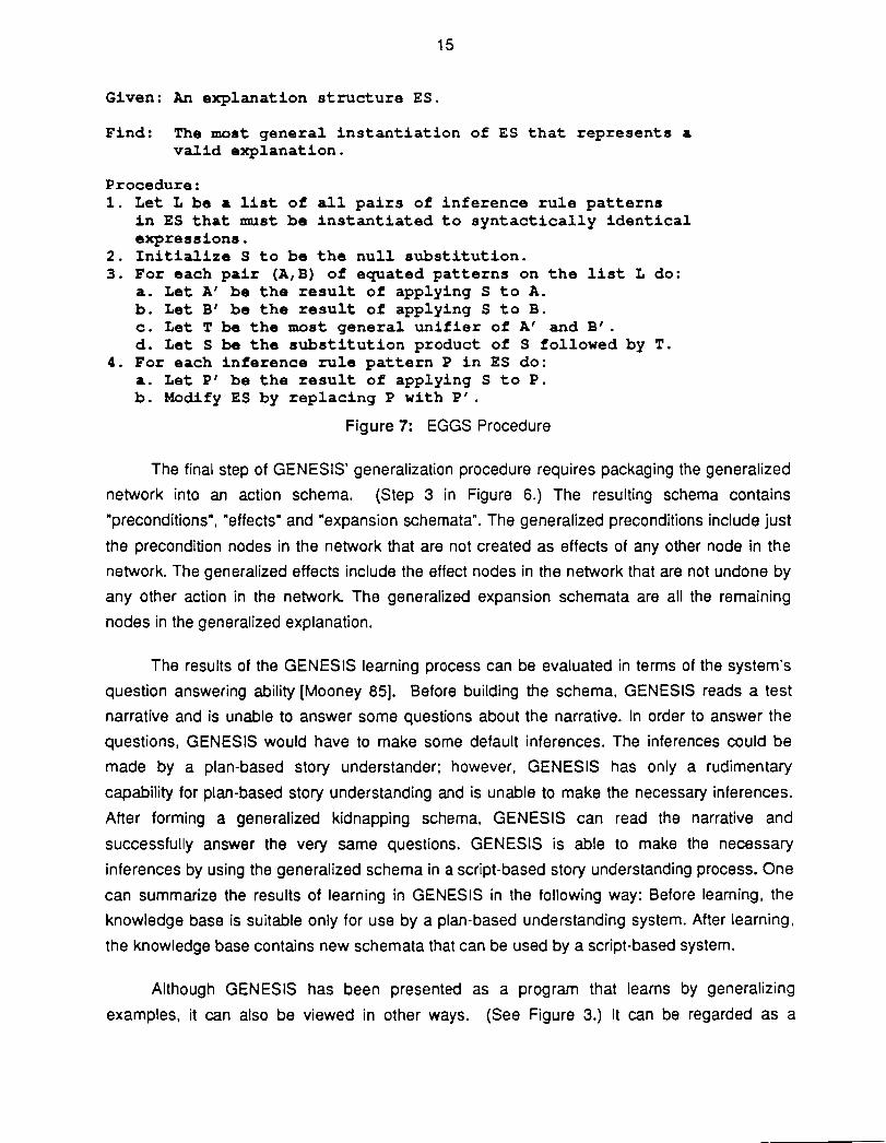
The EGGS procedure takes an explanation structure ES as its input. EGGS is charged

with the task of finding the most general instantiation of ES that represents a valid explanation.

In order that ES represent a valid explanation, the rule patterns must be re-instantiated to some

degree. In particular, if R1 and R2 are two rules incident on a given node of ES, then the

appropriate patterns from R1 and R2 must be instantiated to syntactically identical

expressions.S EGGS first forms a list of all pairs of patterns that must be instantiated to identical

expressions. Then EGGS finds the maximally general set of bindings for the pattern variables

that will simultaneously unify all equated pairs of patterns. Finally, all the rule patterns in ES are

instantiated with these bindings. The resulting network is the most general instantiation of ES

that represents a valid explanation.

After the EGGS procedure is applied to the kidnapping explanation, some of the objects

are generalized and others are constrained. For example, the locations in the "hold-captive"

and "bargain" schemata are generalized. The amount of money is constrained to be any amount

possessed by the target of the kidnapping. The victim of the "capture" schema is constrained to

be the same person mentioned in the "positive-ipt" schema. The resulting generalized

explanation network is shown in Figure 8, taken from [Dejong and Mooney 86].

4The algorithm shown in Figure 7 most closely resembles the version of EGGS presented in [Mooney and Bennett 86); however Mooney and Bennett's presentation apparently contains an error, omitting steps (3a) and (3b) shown in Figure 7.

SAn additional constraint is mentioned in [Mooney 85]. This constraint requires that the pattern representing the main goal of the story match a thematic goal pattern.

15

Given: An explanation structure ES.

Find: The most genera1 instantiation of ES that represents a va1id exp1anation.

Procedure: 1. Let L be a list of a1l pairs of inference ru1e patterns

in ES that must be instantiated to syntactica11y identica1 expressions.

2. Initia1ize S to be the nu11 substitution. 3. For each pair (A,B) of equated patterns on the 1ist L do:

a. Let A' be the result of app1ying S to A. b. Let B' be the result of applying S to B. c. Let T be the most genera1 unifier of A' and B' . d. Let S be the substitution product of S fo11owed by T.

4. For each inference ru1e pattern P in ES do: a. Let P' be the resu1t of applying S to P. b. Modify ES by rep1acing P with P' .

Figure 7: EGGS Procedure

The final step of GENESIS' generalization procedure requires packaging the generalized

network into an action schema. (Step 3 in Figure 6.) The resulting schema contains

"preconditions", "effects" and "expansion schemata". The generalized preconditions include just

the precondition nodes in the network that are not created as effects of any other node in the

network. The generalized effects include the effect nodes in the network that are not undone by

any other action in the network. The generalized expansion schemata are all the remaining

nodes in the generalized explanation.

The results of the GENESIS learning process can be evaluated in terms of the system's

question answering ability [Mooney 85]. Before building the schema, GENESIS reads a test

narrative and is unable to answer some questions about the narrative. In order to answer the

questions, GENESIS would have to make some default inferences. The inferences could be

made by a plan-based story understander; however, GENESIS has only a rudimentary

capability for plan-based story understanding and is unable to make the necessary inferences.

After forming a generalized kidnapping schema, GENESIS can read the narrative and

successfully answer the very same questions. GENESIS is able to make the necessary

inferences by using the generalized schema in a script-based story understanding process. One

can summarize the results of learning in GENESIS in the following way: Before learning, the

knowledge base is suitable only for use by a plan-based understanding system. After learning,

the knowledge base contains new schemata that can be used by a script-based system.

Although GENESIS has been presented as a program that learns by generalizing

examples, it can also be viewed in other ways. (See Figure 3.) It can be regarded as a

16

POSSESS' ~

p GOAl.-PRIORIT Y5_POS iT :VE-IPTI p

~OSSESS9 ~ 3;.FlGAINl

: ""El.D-C;.PT:vE1 ~ :> ~;'PTUFlEl_ -"EEl

9El.IEF8~COMMUNICATE' - BEl.IE-9 p

p BELIEF1S

BELIEF13 _ BELIEF14

GOAL-PRIORITY4"":- GOAl.9

POSSESS9 P"non I hal ~on.y I. BARGAI!"" Penonl mak ... bargaln4"h Penonlln which P.rsonl r<ieas .. Penon) and

Perronl ii,," ~ton<'ll '0 Personl POSSESSI4 Penonl hal Moneyl. GOAL·PRIORITY' Penon! ".n" Perron) Ir« more ,h.n he "'ann '0 h.,. Money!. POSITIVE·IPTI There ,~ a po",,,e In,cr~son~ rtl.tlonshlp OCI"*een Perron2 and Person). HELD·CAPTIIiEI Penonl 15 holdlns Penon) ,ap"". CAPTt:REI Penon I cap,ur .. Person). FREE I Perron) " Ir« BELIEFS Perron2 beli .... Penonl " holdin, P.non) ,:aptl". COMMLNICATE I Pe...,nl conl1ces Pcrronl .nd ,ells him ,h.t h. " holdin& Person) captl' •. BELlEF9 Person I beh., .. h. u holdlns P""on) c.p,,' •.

BELIEFI) Pononl beh .... Pcrsonl "&n .. Perron) '0 be Ir« more th.n he w.n's '0

h.,. Money I.

BELIEFI. Perron I beh .... 'here IS. pos",'. In,erpersonal r.latlonshlp bet"'«n Penonl

GOAL·PRIORITY. P .. ronl ".nll 10 h ••• Moneyl more than h .... nes to hold Person) c'p,,'e. GOAL9 Perronl .... n" 10 h.,. Moneyl

Figure 8: The Generalized Kidnapping Network

chunking system, which learns by combining operators into macro operators. The generalized

kidnapping schema may be viewed as a macro operator composed of the ·capture·,

·communicate· and "bargain" operators. GENESIS may also be viewed as a system that

reformulates non-operational concept deSCriptions. Before learning, the system may be said to

possess a non-operational description of the concept ·plans for obtaining money·. The pattern

describing the thematic goal "obtain money·, together with the knowledge base of action

schemata, could be viewed as a non-operational specification of the collection of all plans for

obtaining money. The description is non-operational since the information about what

constitutes a valid plan for obtaining money is scattered throughout the knowledge base. After

learning, GENESIS has an operational description of the concept. in the form of a general

schema. The schema explicitly describes a set of plans. Any instantiation of the generalized

schema is a valid plan for obtaining money.

17

3.2.2 The LEX-II System (Mitchell and Utgoff)

Another major effort to investigate EBl techniques has been undertaken by Mitchell and

coworkers at Rutgers University. A number of different EBl systems have been developed by

Mitchell's group [Mitchell et al. 86; Mitchell 83a; Mitchell 82b; Mitchell et al. 83; Utgoff 86; Utgoff

82; Keller 83; Mahadevan 85; Kedar-Cabelli 85; Williamson 85]. One of the oldest of these

systems is lEX-II, which learns search control heuristics in the domain of symbolic integration.

lEX-II was built as an extension to the lEX-I system. lEX-I uses purely empirical (SBl)

techniques for learning concepts from multiple examples [Mitchell 83b; Mitchell 81]. lEX-II was

built to combine the empirical techniques of lEX-I with analytical (EBl) learning methods for

generalizing from single examples [Mitchell 83a; Mitchell 82b].

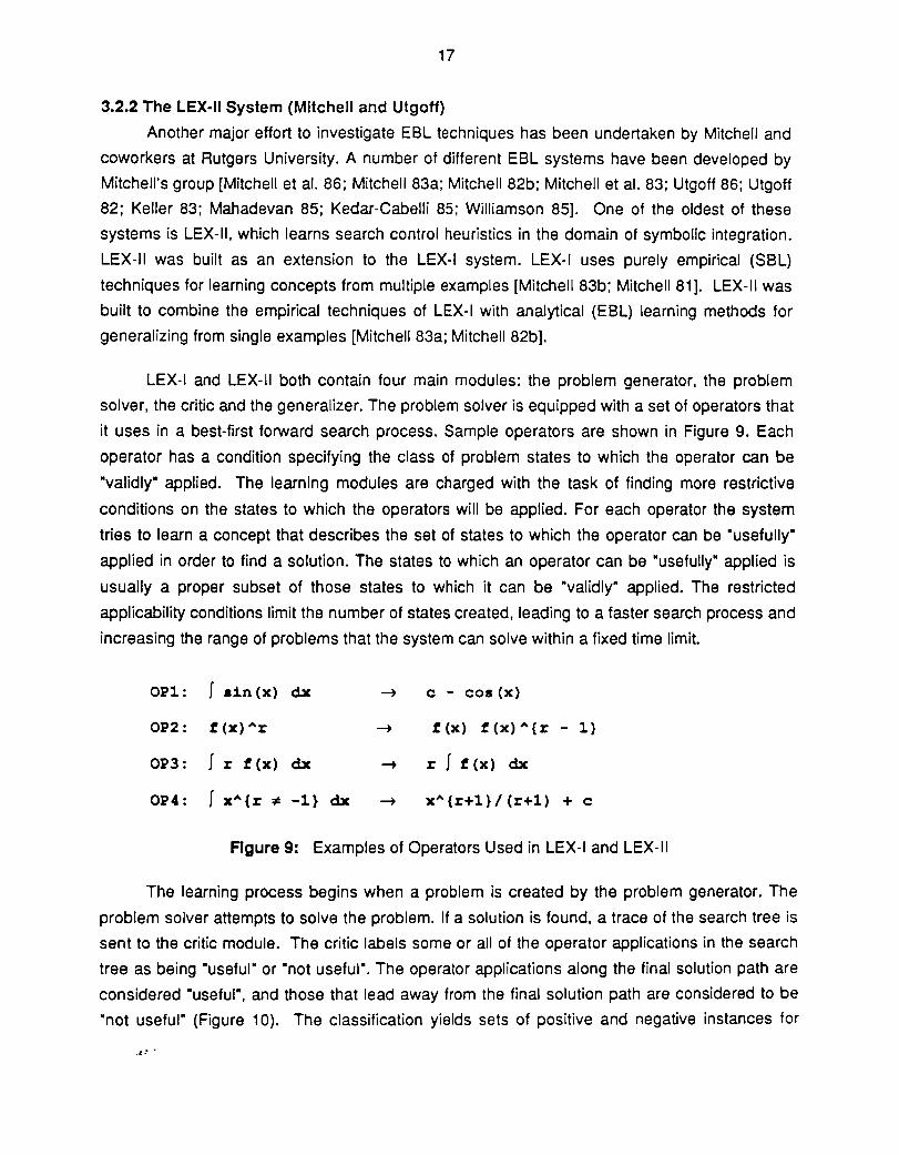
lEX-I and lEX-II both contain four main modules: the problem generator, the problem

solver, the critic and the generalizer. The problem solver is equipped with a set of operators that

it uses in a best-first forward search process. Sample operators are shown in Figure 9. Each

operator has a condition speCifying the class of problem states to which the operator can be

"validly" applied. The learning modules are charged with the task of finding more restrictive

conditions on the states to which the operators will be applied. For each operator the system

tries to learn a concept that describes the set of states to which the operator can be "usefully·

applied in order to find a solution. The states to which an operator can be "usefully" applied is

usually a proper subset of those states to which it can be ·validly· applied. The restricted

applicability conditions limit the number of states created, leading to a faster search process and

increasing the range of problems that the system can solve within a fixed time limit.

OP1: f sin (x) dx ~ c - cos (x)

OP2: f(x)Ar ~ f (x) f (x) A {r - 1}

OP 3 : f r f (x) dx ~ r f f (x) dx

OP 4 : f XA {r ~ -1} dx x A {r+1}/(r+1) + c

Agure 9: Examples of Operators Used in lEX-I and lEX-II

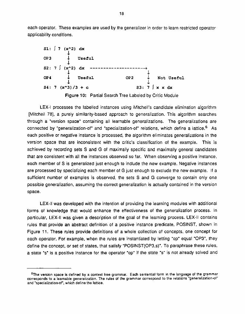
The learning process begins when a problem is created by the problem generator. The

problem solver attempts to solve the problem. If a solution is found, a trace of the search tree is

sent to the critic module. The critic labels some or all of the operator applications in the search

tree as being "useful" or "not useful". The operator applications along the final solution path are

considered "useful", and those that lead away from the final solution path are considered to be

"not useful" (Figure 10). The classification yields sets of positive and negative instances for

I.: .

18

each operator. These examples are used by the generalizer in order to learn restricted operator

applicability conditions.

Sl: f 7 (x"2) dx i

OP3 i Useful i

S2: 7 J (x"2) dx --------------------~ i i

OP4 i Useful OP2 i Not Useful i i

S4: 7 (x"3) /3 + c S3: 7 f x x dx

Figure 10: Partial Search Tree Labeled by Critic Module

LEX-I processes the labelled instances using Mitchell's candidate elimination algorithm

[Mitchell 78], a purely similarity-based approach to generalization. This algorithm searches

through a "version space" containing all learnable generalizations. The generalizations are

connected by "generalization-of" and "specialization-of" relations, which define a lattice.6 As

each positive or negative instance is processed, the algorithm eliminates generalizations in the

version space that are inconsistent with the critic's classification of the example. This is

achieved by recording sets Sand G of maximally specific and maximally general candidates

that are consistent with all the instances observed so far. When observing a positive instance,

each member of S is generalized just enough to include the new example. Negative instances

are processed by specializing each member of G just enough to exclude the new example. If a

sufficient number of examples is observed, the sets Sand G converge to contain only one

possible generalization, assuming the correct generalization is actually contained in the version

space.

LEX-II was developed with the intention of providing the learning modules with additional

forms of knowledge that would enhance the effectiveness of the generalization process. In

particular, LEX-II was given a description of the goal of the learning process. LEX-II contains

rules that provide an abstract definition of a positive instance predicate, POSINST, shown in

Figure 11. These rules provide definitions of a whole collection of concepts, one concept for

each operator. For example, when the rules are instantiated by letting MOp" equal "OP3", they

define the concept, or set of states, that satisfy ·POSINST(OP3,s)". To paraphrase these rules,

a state "s" is a positive instance for the operator MOp· if the state Os· is not already solved and

6The version space is defined by a context free grammar. Each sentential form in the language of the grammar corresponds to a leamable generalization. The rules of the grammar correspond to the relations "generalization-of­and "specialization-of", which define the lattice.

19

applying HOp· to OS" leads to a state that is either solved or is solvable by additional operator

appl ications.

(~op,s){POSINST(op,s) ¢= USEFUL(op,s)}

(~op,s){USEFUL(op,s) ¢= [~SOLVED(s) A SOLVABLE(APPLY(op,s»]}

(~op,s){SOLVABLE(s) ¢= SOLVABLE(APPLY(op,s)}

(~op,s){SOLVABLE(s) ¢= SOLVED(APPLY(op,s)}

Figure 11: Rules Defining the POSINST Predicate in LEX-II

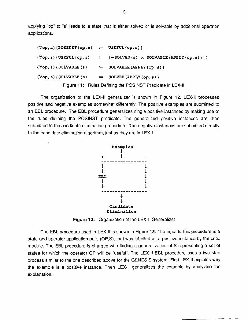
The organization of the LEX-II generalizer is shown in Figure 12. LEX-II processes

positive and negative examples somewhat differently. The positive examples are submitted to

an EBL procedure. The EBL procedure generalizes single positive instances by making use of

the rules defining the POSINST predicate. The generalized positive instances are then

submitted to the candidate elimination procedure. The negative instances are submitted directly

to the candidate elimination algorithm. just as they are in LEX-I.

Examples .L

+ .L

.L

.L CancU.date

Elimination

Figure 12: Organization of the LEX-II Generalizer

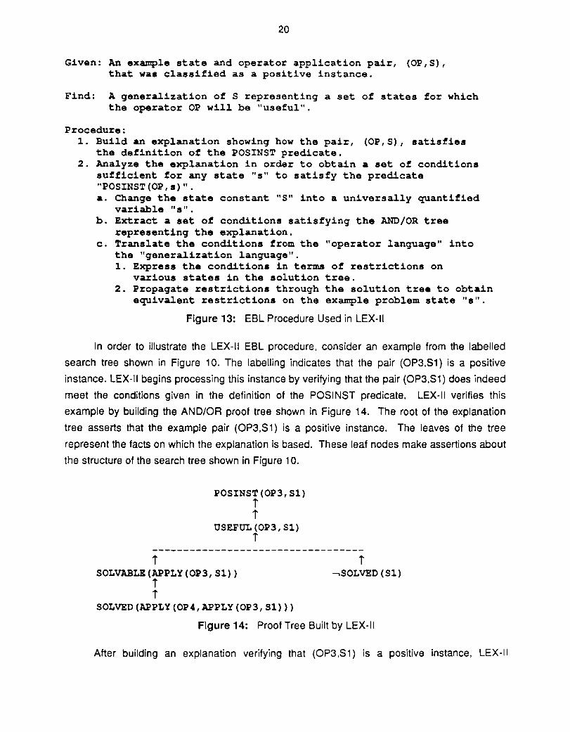
The EBL procedure used in LEX-II is shown in Figure 13. The input to this procedure is a

state and operator application pair. (OP.S). that was labelled as a positive instance by the critic

module. The EBL procedure is charged with finding a generalization of S representing a set of

states for which the operator OP will be "useful". The LEX-II EBL procedure uses a two step

process similar to the one described above for the GENESIS system. First LEX-II explains why

the example is a positive instance. Then LEX-II generalizes the example by analyzing the

explanation.

20

Given: An example state and operator application pair, (OP,S), that was classified as a positive instance.

Find: A generalization of S representing a set of states for which the operator OP will be "useful".

Procedure: 1. Build an explanation showing how the pair, (OP,S), satisfies

the definition of the POSINST predicate. 2. Analyze the explanation in order to obtain a set of conditions

sufficient for any state "s" to satisfy the predicate "POSINST(OP,s)". a. Change the state constant "S" into a universal.ly quantified

variable "s". b. Extract a set of conditions satisfying the AND/OR tree

representing the explanation. c. Translate the conditions from the "operator language" into

the "general.ization language". 1. Express the conditions in terms of restrictions on

various states in the solution tree. 2. Propagate restrictions through the solution tree to obtain

equivalent restrictions on the example problem state "s".

Figure 13: EBL Procedure Used in LEX-II

In order to illustrate the LEX-II EBL procedure, consider an example from the labelled

search tree shown in Figure 10. The labelling indicates that the pair (OP3,S1) is a positive

instance. LEX-II begins processing this instance by verifying that the pair (OP3,S1) does indeed

meet the conditions given in the definition of the POSINST predicate. LEX-II verifies this

example by building the AND/OR proof tree shown in Figure 14. The root of the explanation

tree asserts that the example pair (OP3,S 1) is a positive instance. The leaves of the tree

represent the facts on which the explanation is based. These leaf nodes make assertions about

the structure of the search tree shown in Figure 10.

POSINST(OP3,Sl) i i

OSEFUL(OP3,Sl) i

i SOLVABLE(APPLY(OP3,Sl»

i i

SOLVED(APPLY(OP4,APPLY(OP3,Sl»)

i .....,SOLVED (Sl)

Figure 14: Proof Tree Built by LEX-II

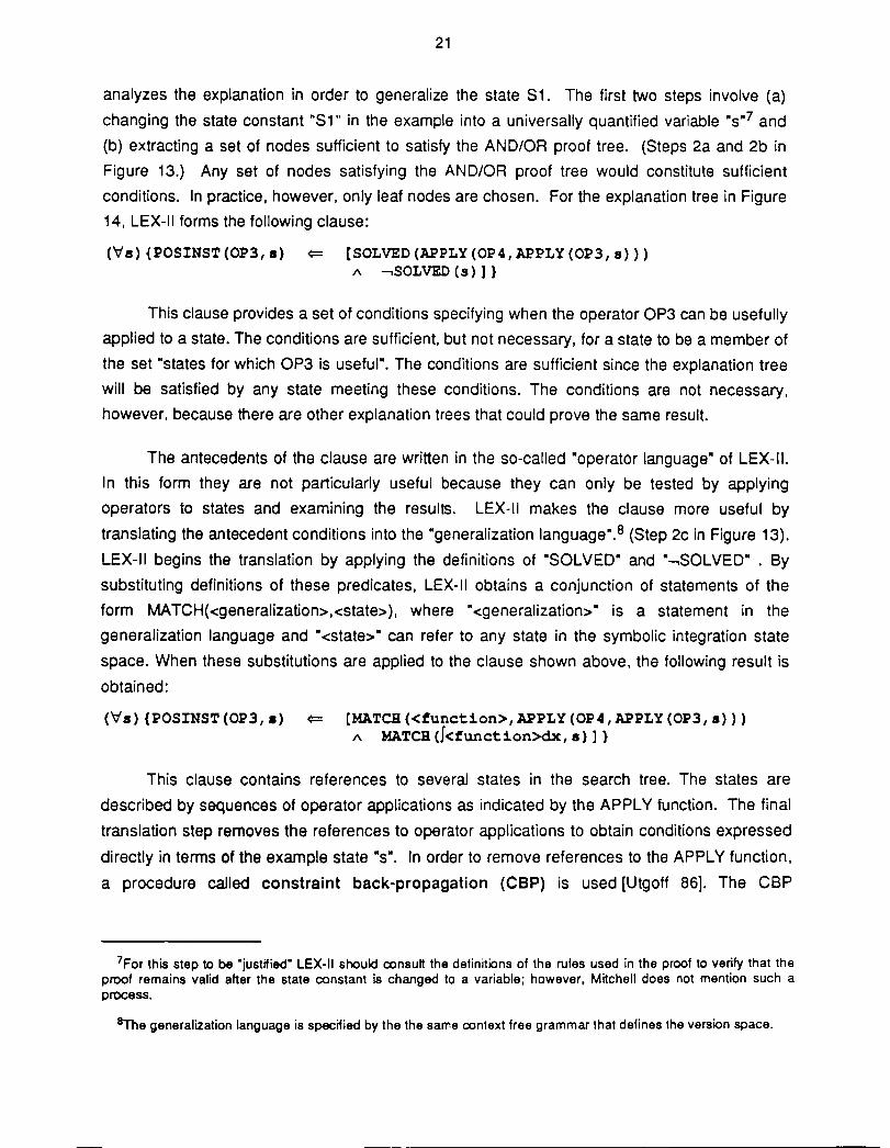
After building an explanation verifying that (OP3,S1) is a positive instance, LEX-II

21

analyzes the explanation in order to generalize the state S1. The first two steps involve (a)

changing the state constant "S1" in the example into a universally quantified variable "s"7 and

(b) extracting a set of nodes sufficient to satisfy the ANDIOR proof tree. (Steps 2a and 2b in

Figure 13.) Any set of nodes satisfying the ANDIOR proof tree would constitute sufficient

conditions. In practice, however, only leaf nodes are chosen. For the explanation tree in Figure

14, LEX-II forms the following clause:

(~s){POSINST(OP3,a) ¢= [SOLVED(APPLY(OP4,APPLY(OP3,s») 1\ -.SOLVED (s) ] }

This clause provides a set of conditions specifying when the operator OP3 can be usefully

applied to a state. The conditions are sufficient, but not necessary, for a state to be a member of

the set ·states for which OP3 is useful". The conditions are sufficient since the explanation tree

will be satisfied by any state meeting these conditions. The conditions are not necessary,

however, because there are other explanation trees that could prove the same result.

The antecedents of the clause are written in the so-called "operator language" of LEX-II.

In this form they are not particularly useful because they can only be tested by applying

operators to states and examining the results. LEX-II makes the clause more useful by

translating the antecedent conditions into the "generalization language".s (Step 2c in Figure 13).

LEX-II begins the translation by applying the definitions of "SOLVED" and "-,SOLVED" . By

substituting definitions of these predicates, LEX-II obtains a conjunction of statements of the

form MATCH{<generalization>,<state», where "<generalization>" is a statement in the

generalization language and "<state>· can refer to any state in the symbolic integration state

space. When these substitutions are applied to the clause shown above, the following result is

obtained:

(~a){POSINST(OP3,.) ¢= [HATCH«tunction>,APPLY(OP4,APPLY(OP3,s») 1\ HATCH d<tunction>dx, a)] }

This clause contains references to several states in the search tree. The states are

described by sequences of operator applications as indicated by the APPLY function. The final

translation step removes the references to operator applications to obtain conditions expressed

directly in terms of the example state ·s·. In order to remove references to the APPLY function,

a procedure called constraint back-propagation (CBP) is used [Utgoff 86]. The CBP

7For this step to be "justified" LEX-II should consult the definitions of the rules used in the proof to verify that the proof remains valid after the state constant is changed to a variable; however, Mitchell does not mention such a process.

liThe generalization language is specified by the the same context free grammar that defines the version space.

22

technique is given the task of translating any statement in the form MATCH(P.APPLY(OP,s))

into an equivalent statement of the form MATCH(P',s). This is essentially equivalent to

calculating "weakest preconditions" as formalized in [Dijkstra 76] and to performing

goal-regression [Nilsson 80; Waldinger 77]. The pattern P' must meet the requirement that a

state S will match P' if and only if the state APPLY(OP,S) matches P. The CBP procedure is

implemented by writing one LISP function for each problem solving operator. The LISP function

represents the "inverse" of that operator.9The inverse for operator OP would take a pattern such

as P and find the corresponding weakest precondition p'.10 After applying the CBP procedure to

the antecedents in the clause shown above, the following result is obtained.

('Va) {POSINST(OP3,s) ~ [MATCH(Jr(x"'{r ~ -l})dx,a) 1\ MATCH <f<function>dx, s)] }

The power of the LEX-II generalization procedure can be illustrated by comparing this

result to the original example shown in Figure 10. The original example only asserted the

usefulness of applying operator OP3 to the single problem state S1. The clause shown above

asserts the usefulness of applying operator OP3 to a larger class of problem states. Two

distinct generalizations have been made. The coefficient "7" has been generalized to "r", any

real number. Furthermore, the exponent "2" has been generalized to any real number "I"', other

than "-1".

The final generalization step involves combining the results of (EBL) generalization of

single positive examples with the (SBL) candidate elimination algorithm. The generalization

shown above provides sufficient (but not necessary) conditions for concept membership.

Therefore, every candidate generalization must be at least as general as this generalized

postive instance. For this reason, the generalized instance can be processed by the candidate

elimination algorithm just as if it were an actual positive instance. The algorithm must simply

generalize each member of the boundary set S just enough to include the generalized positive

instance.

Although lEX-II does not use its EBl techniques to process negative examples, there is

no reason in principle why this cannot be done. The system could be provided with a set of

9Strictly speaking, these LISP functions are not true inverses of the corresponding operators. If OP maps problem states to problem states, the true inverse would map states to states. The so-called "inverse" used here maps patterns (sets of states) to other patterns.

lOA difficulty arises when the precondition P' cannot be expressed in the generalization language of LEX·II. When this happens, the system defines new terms to expand the generalization language so it can express the desired precondition (Utgoff 86). On one occasion the system was led to define a new term equivalent to "odd integer" in order to resolve such an impasse.

~ ...

23

rules for proving statements of the form -.POSINST(OP,S). By processing explanations of

negative instances, the system could obtain generalized negative instances. These could be

used to refine the boundary set G, just as generalized positive instances are used to refine the

boundary set S. In practice, explanations of negative instances would be large and difficult to

analyze if the predicate POSINST is defined as above. A proof of -.POSINST(OP,S) would

require showing that the state APPLY(OP,S) is a dead end. This would mean proving that no

operators apply or that all applicable operators lead to other dead end states. The proof might

have to reason about a large number of states in the search tree. Proofs of POSINST need only

reason about states along a Single solution path.

The value of using EBL techniques in LEX-II can be assessed by observing the rate at

which learning occurs. The candidate elimination algorithm should converge faster in LEX-II

than in LEX-I, because LEX-II uses generalized positive instances to refine the boundary set

S. The EBL techniques effectively provide a stronger bias for inductive learning. LEX-I makes

use of the bias contained in the definition of the generalization language. LEX-II uses this bias in

addition to the constraints provided by using EBL techniques to generalize positive instances.

The stronger bias and faster rate of convergence should lead to improved performance by the

problem solver, since the learned heuristics are available earlier in LEX-II than in LEX-/'

The learning component of LEX-II was able to improve the overall problem solving

performance of the system during the initial stages of learning. Eventually a point was reached

after which the acquisition of new heuristics failed to improve the overall performance of the

system [Mitchell 83a]. The difficulty results from the fact that the heuristics learned by LEX-II are

capable of improving only some aspects of the system's performance. Heuristics help decide

what operator to apply, given a state to be expanded. They do not provide direct guidance about

what state should be chosen for expansion. Eventually the system's performance was limited by

the decision of which state to expand, rather than which operator to apply. This "wandering

bottleneck" problem results from the fact that only some aspects of the system's performance

fall within the scope of the learning module.

Although LEX-II has been presented mainly as a system for generalizing from examples.

it can also be viewed in other ways. (See Figure 3.) LEX-II can be viewed as a system that

performs "chunking" of operator sequences to form macro operators. In the example shown

above the system learns a condition describing the set of states for which the sequence OP3

followed by OP4 will lead to a solved state. The system could save this macro in a memory

along with its applicability condition. Although LEX-II does not actually save such macro

operators, it could easily be extended to do so.

24

lEX-II can also be viewed as a system that reformulates non-operational concept

descriptions. In the example shown above the system translates the concept

"POSINST(OP3,s)" into a conjunction of patterns in system's generalization language. lEX-II

could, in principle, be modified to reformulate concepts other than the POSINST predicate

defined in Figure 11. As described in [Mitchell 82b], the rules defining POSINST could be

changed so that an operator application is considered to be useful only if it lies along a minimum

cost path to a solution; however, this change was apparently never implemented. Were the

rules so modified, they would probably lead to large and complex explanations that would be

difficult to analyze, just as explanations for negative instances would be difficult to analyze.

Proving a path to be minimal in cost would require reasoning about an entire search tree, rather

than merely reasoning about a single solution path.

3.2.3 Similar Work

Several other investigators have developed EBl systems that are naturally viewed in

terms of generalizing from examples. Minton has implemented a variant of EBl called

"constraint-based generalization" [Minton 84]. He has used the method in a program that learns

forced win positions in games like tic-tac-toe, go-moku and chess. Two similar EBl systems

that operate in the domain of logic circuit design were developed independently by Ellman

[Ellman 85] and Mahadevan [Mahadevan 85]. Ellman's program is capable of generalizing an

example of a shift register into a schema describing devices for implementing arbitrary bit

permutations. The schema is created by a process that analyzes the proof of correctness of the

example circuit. Mahadevan's method is called -verification-based learning- (VBl). The VBl

technique is intended to be a general method of learning problem decomposition rules.

Mahadevan has tested VBl in the domains of logiC circuit design and symbolic integration.

Williamson is using EBl methods in a system to learn exceptions to semantic integrity

constraints in databases [Williamson 85].

A number of people working with DeJong have also developed new EBl systems

following up on GENESIS. O'Rorke is developing a -Mathematicians Apprentice" (MA) using

techniques similar to GENESIS [O'Rorke 84; O'Rorke 85]. The MA program uses explanation­

based methods to create schemata summarizing successful theorem proving episodes. Shavlik

is building a system that learns concepts trom classical phYSics [Shavlik 85a; Shavlik and

Dejong 85; Shavlik 85b]. His "PHYSICS 101" system is intended to learn concepts like

conservation of momentum, starting with only a knowledge of Newton's laws and calculus.

Segre is working on a system that uses EBl methods to learn schemata describing robot

manipulator sequences [Segre 85; Segre and DeJong 85].

25

3.3 EBl = Chunking Chunking is usually understood in the context of problem spaces. problem states and

operators. A chunking system takes a linear or tree structured sequence of operators as its

input. The task of the chunking system is to convert the sequence of operators into a single

"macro-operator". or ·chunk". that has the same effect as the entire sequence. This process is

sometimes described as "compiling" the operator sequence.

As shown in Figure 3. chunking can be placed into rough correspondence with the EBL

generalization techniques described in the preceding section. The process of forming an

operator sequence out of primitive operators is analogous to forming an explanation out of

explanation rules. Compiling an operator sequence into a macro corresponds to analyzing and

generalizing an explanation. Problem states may be seen to play the role of training examples.

The chunking process produces a precondition for the macro operator. The macro precondition

represents a generalization of the example state. It is also possible to view an instantiated

operator sequence as a training example and view a generalized operator sequence as the

learned concept.

3.3.1 The SOAR System (Rosenbloom, Laird and Newell)

The SOAR project is an ambitious attempt to build a system combining learning and

problem solving capabilities into an architecture for general intelligence [Laird et al. 86; Laird et

aI. 84]. The problem solving methods in SOAR are based on "universal subgoaling" (USG)

[Laird 84] and the "universal weak method" (UWM) [Laird 83; Laird and Newell 83]. Universal

subgoaling is a technique for making all search control decisions in a uniform manner. The

universal weak method is an architecture that provides the functionality of all the weak methods

[Newell 69]. The learning strategy of SOAR is based on the technique for "chunking"

sequences of production rules that was developed by Rosenbloom and Newell [Rosenbloom

and Newell 86; Rosenbloom 83]. The developers of SOAR claim that chunking is a universal

learning method. They also believe that chunking techniques are especially powerful when

combined with the USG and UWM architecture.

The architecture of SOAR is based on the "problem space hypothesis" [Newell 80]. the

notion that all intelligent activity occurs in a problem space. This idea is embodied in SOAR by

allowing all decisions to be made in a single uniform manner. i.e .. by searching in a problem

space. At any point in time SOAR is working in a ·current context" that describes the status of

the search in whatever problem space SOAR is currently using. More specifically. the current

context consists of four parts: a goal. a space. a state and an operator. The current context can

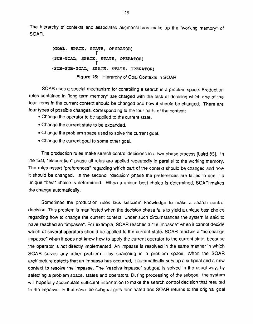
be linked to previous contexts so that a goal and subgoal hierarchy is formed (Figure 15). The

components of each context are annotated with additional information called "augmentations".

26

The hierarchy of contexts and associated augmentations make up the "working memory" of

SOAR.

(GOAL, SPACE, STATE, OPERATOR) i

(SOB-GOAL, SPACE, STATE, OPERATOR) i

(SOB-SOB-GOAL, SPACE, STATE, OPERATOR)

Figure 15: Hierarchy of Goal Contexts in SOAR

SOAR uses a special mechanism for controlling a search in a problem space. Production

rules contained in "long term memory" are charged with the task of deciding which one of the

four items in the current context should be changed and how it should be changed. There are

four types of possible changes. corresponding to the four parts of the context:

• Change the operator to be applied to the current state.

• Change the current state to be expanded.

• Change the problem space used to solve the current goal.

• Change the current goal to some other goal.

The production rules make search control decisions in a two phase process [Laird 83]. In

the first. "elaboration" phase all rules are applied repeatedly in parallel to the working memory.

The rules assert "preferences· regarding which part of the context should be changed and how

it should be changed. In the second. "decision" phase the preferences are tallied to see if a

unique "best" choice is determined. When a unique best choice is determined. SOAR makes

the change automatically.

Sometimes the production rules lack sufficient knowledge to make a search control

decision. This problem is manifested when the decision phase fails to yield a unique best choice

regarding how to change the current context. Under such circumstances the system is said to

have reached an "impasse". For example, SOAR reaches a "tie impasse" when it cannot decide

which of several operators should be applied to the current state. SOAR reaches a "no change

impasse" when it does not know how to apply the current operator to the current state. because

the operator is not directly implemented. An impasse is resolved in the same manner in which

SOAR solves any other problem - by searching in a problem space. When the SOAR

architecture detects that an impasse has occurred. it automatically sets up a subgoal and a new

context to resolve the impasse. The "resolve-impasse" subgoal is solved in the usual way, by

selecting a problem space. states and operators. During processing of the subgoal, the system

will hopefully accumulate sufficient information to make the search control decision that resulted

in the impasse. In that case the subgoal gets terminated and SOAR returns to the original goal

27

and context.

In order to illustrate the behavior of SOAR. consider the following example of solving the

8-PUZZLE. The a-PUZZLE involves moving tiles around on a rectangular grid. The initial state

and goal state for the puzzle are shown in Figure 16. taken from [Laird et al. 86]. In order to

solve the puzzle. one must find a sequence of tile moves that transforms the initial state into the

goal state. A partial trace of SOAR's solution is shown in Figure 17, taken from [Laird et al. 86].

SOAR starts with the goal "SOLVE-EIGHT-PUZZLE". An abstract problem space called

"EIGHT-PUZZLE-SD" is selected. The operators of the abstract space are called ·PLACE­

BLANK", "PLACE-1", "PLACE-2", etc. Each such abstract operator is intended to achieve the

function of moving one particular tile or the space to its goal position. SOAR chooses the

operator "PLACE-BLANK" first. A "NO-CHANGE" impasse occurs because the abstract

operator is not implemented and SOAR does not know how to apply it to the current state. A

"RESOLVE-NO-CHANGE" goal to is created for the purpose of resolving the impasse. SOAR

attempts to solve the new goal by working in the original "EIGHT-PUZZLE" problem space.

Another impasse occurs later when SOAR cannot decide which of the three operators, "LEFT".

"UP" or "DOWN", to apply. This leads to a new subgoal. and so on. The system eventually

accumulates enough information to resolve the sequence of impasses and their associated

subgoals. This occurs by line 16 when SOAR has tried applying the operator "LEFT" and

discovers that the blank is now in its correct location. This means that SOAR has now found a

way to apply the abstract operator "PLACE-BLANK" to this particular initial state.

Oes"f!'!l Slatl!

2 J I I 2 J

a ~ a ~

. 6 5 7 6 5

Flgure 16: Initial and Goal States for a-Puzzle

The learning mechanism in SOAR is intended to acquire search control knowledge from

problem solving experience. In particular. the chunking system creates new production rules

that help SOAR to make search control decisions more easily. The new rules enable SOAR to

make such decisions directly through the elaboration and decision phases described above.

The result is that fewer impasses occur and SOAR avoids the need to process subgoals. The

28

'~1 tol .. ,-,t.''I!-g:...t.t1. PI ,';ht-culzl.-sa S I

, ':;)1 olael-blank •• ~G2 (r.sol •• -~c-e~.n;.)

P2 ,1Qftt"P,JIZ't

7 51 9 •• >G3 (rlsohl-ti. ~Hl.rltor)

• P3 t1t 10 52 ('"ft .• p. aeln} II 06 1,.I."tl-eoJ"ct(02('"ft» 12 •• )G. (r.soly.-~o-c~.ng.) Il PZ 11~ht-p",,11

I' 51 15 OZ , 1ft 15 5J

11 02 lIn IS 5' Ii 5' 20 O' plleo-I

Figure 17: Trace of SOAR Execution on 8-Puzzle

chunking mechanism operates continuously. Whenever a subgoal terminates in SOAR, the

chunking mechanism is invoked. 11 The mechanism attempts to build a new rule that will

summarize the results of the processing the subgoal. When the same subgoal occurs in an

identical or similar situation, the new rule will fire and help make a decision that previously led to

an impasse.

The chunking procedure is described in [Laird et al. 86] and outlined in Figure 18_

Assuming a subgoal G has just terminated, the chunking process will create a new production

rule R having the same effect as the entire sequence of production rules that fired during the

processing of goal G. The first step involves collecting conditions and actions for the new rule

R. The conditions are found on a -referenced list- that was maintained during the processing of

goal G. The "referenced Iisf contains all working memory elements that were created before

goal G and were referenced by rules that fired during the processing of G. If these working

memory elements were to be present in some other situation, they would enable the same

"This capability requires that the system meet the "goaJ-architecturality constraint", i.e., the representation of goals must be defined in the system architecture itself [Rosenbloom and Newell 86].

29

sequence of rules to fire. 12 These working memory elements become the conditions of the new

rule R. The actions of R are found by determining which working memory elements were

created during processing of goal G and were passed on to supergoals of G by being attached

as augmentations to the context of a supergoal of G. These actions are just the information that

was remembered by the system after goal G was terminated. They constitute the information

required to resolve the impasse that led to the creation of goal G.

In order that the new rule R be applicable to a variety of situations, some of the constants

in the conditions and actions of R need to be generalized. In particular the "identifiers· must be

changed to variables. This is necessary since each identifier is unique to a working memory

element. In order to choose variables, SOAR must determine which identifiers are required to

be equal to each other and which are required to be distinct. The procedure shown in Figure 18

makes the decision in a conservative way leading to chunk applicability conditions that are as

restrictive as possible. It assumes that equal identifiers in the example are required to be equal

and replaces them with a single variable. It also assumes that distinct identifiers in the example

are required to be distinct and replaces them with distinct variables. An additional constraint is

added to guarantee that distinct variables match distinct identifiers. The developers of SOAR

claim this approach guarantees that no over-generalized rules will be created, although over­

specialized rules will sometimes be formed [Laird et al. 86]. The final step in Figure 18 involves

making the new rule more efficient by reordering the conditions and making other changes for

the sake of efficiency.

The chunking mechanism in SOAR has gone through several implementations. An earlier

implementation used a different criterion for deciding when chunking should occur [Rosenbloom

and Newell 86]. The earlier criterion specified that chunking take place only for goals that were

solved without invocation of subgoals. This resulted in "bottom-up" chunking, which was useful

for cognitive modelling. A recent implementation uses a different method of finding the

conditions that go into a rule created by the chunking mechanism [Laird et al. 86]. The new

approach involves tracing dependencies from the results of a goal, through the sequence of

rules that fired, back to working memory elements present before the goal was created. This

approach leads to rules with greater generality than the one described above. The new method

excludes conditions that were referenced by production rules that fired but did not contribute to

12Strictly speaking, this requires that the system meet the "crypto-information constraint", i.e., the firing of rules must not be controlled by "hidden information" such as a conflict resolution strategy [Rosenbloom and Newell 86].

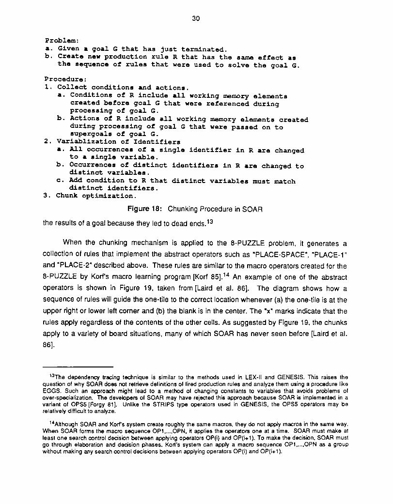
30

Problem: a. Given a goal G that has just terminated. b. Create new production rule R that has the same effect as

the sequence o~ rules that were used to solve the goal G.

Procedure: 1. Collect conditions and actions.

a. Conditions o~ R include all working memory elements created be~ore goal G that were referenced during processing o~ goal G.

b. Actions o~ R include all working memory elements created during processing of goal G that were passed on to supergoals of goal G.

2. Variablization of Identifiers a. All occurrences of a single identifier in R are changed

to a single variable. b. Occurrences of distinct identifiers in R are changed to

distinct variables. c. Add condition to R that distinct variables must match

distinct identifiers. 3. Chunk optimization.

Figure 18: Chunking Procedure in SOAR

the results of a goal because they led to dead ends. 13

When the chunking mechanism is applied to the 8-PUZZLE problem. it generates a

collection of rules that implement the abstract operators such as "PLACE-SPACE". "PLACE-1"

and "PLACE-2" described above. These rules are similar to the macro operators created for the

8-PUZZLE by Korf's macro learning program [Korf 85].14 An example of one of the abstract

operators is shown in Figure 19. taken from [Laird et al. 86]. The diagram shows how a

sequence of rules will guide the one-tile to the correct location whenever (a) the one-tile is at the

upper right or lower left comer and (b) the blank is in the center. The ·x" marks indicate that the

rules apply regardless of the contents of the other cells. As suggested by Figure 19. the chunks

apply to a variety of board situations. many of which SOAR has never seen before [Laird et al.

86].

'3The dependency tracing technique is similar to the methods used in LEX·II and GENESIS. This raises the question of why SOAR does not retrieve definitions of fired production rules and analyze them using a procedure like EGGS. Such an approach might lead to a method of changing constants to variables that avoids problems of over-specialization. The developers of SOAR may have rejected this approach because SOAR is implemented in a variant of OPS5 [Forgy 81]. Unlike the STRIPS type operators used in GENESIS. the OPS5 operators may be relatively difficult to analyze.

'''Although SOAR and Korfs system create roughly the same macros, they do not apply macros in the same way. When SOAR forms the macro sequence OP1 •...• 0PN. it applies the operators one at a time. SOAR must make at least one search control decision between applying operators OP(i) and OP(i.l). To make the decision. SOAR must go through elaboration and decision phases. Korf's system can apply a macro sequence OP1 ..... 0PN as a group without making any search control decisions between applying operators OP(i) and OP(i.1 ).

31

~" bm" '1;1, _. !, .. (, I • t. -(

Figure 19: Abstract Operator Created by SOAR

In order to evaluate the chunking mechanism in SOAR, it is useful to examine SOAR's

behavior before and after chunking takes place. Figure 17 shows how SOAR behaves before

chunking takes place. SOAR was forced to resolve three impasses in order to apply the

abstract operator "PLACE-BLANK". After learning chunks, SOAR can solve this problem and

similar ones without the occurrence of any impasses. SOAR creates new rules that avoid

impasses and the searching that results from impasses. The question arises as to whether a

reduction in the number of impasses necessarily means an increase in efficiency. Statistics

presented in [Laird et al. 84] address this issue. The chunking method does reduce the total

number of search control decisions that the system must make. Nevertheless, it remains

unclear whether the number of search control decisions is an appropriate unit of measurement.

Chunking can reduce the number of search control decisions by creating rules used in the

elaboration and decision phases. These processes may run more slowly after chunking than

before. The difficult work may simply have been moved to a different part of the system.

The developers of SOAR have claimed that the power of chunking is enhanced when

used in the context of a problem solving architecture such as SOAR [Laird et al. 86], because all

parts of the system fall within the scope of the learning mechanism. They argue that the SOAR

architecture allows chunking to improve any aspect of the behavior of a problem solving system.

This can enable SOAR to avoid -Wandering bottleneck" problems, which have occurred in

systems like LEX-II [Mitchell 83a]. This potential capability results from the fact that all decisions

in SOAR are made In the same manner, by searching in a problem space. The chunking

mechanism can aeate production rules that summarize the results of search. It follows that the

learning system in SOAR has the potential to create rules to guide any of the decisions that the

system makes in the course of problem solving. All decisions can be influenced by the chunking

mechanism. More practical experience is needed to determine whether this conclusion is borne

out in practice.

Although SOAR has been described mainly in terms of chunking, it can also be viewed in

32

other ways. (See Figure 3.) SOAR can also be viewed as a system that can generalize from a

single example. After SOAR solves a goal in one situation, it creates a rule that can solve the

same goal when it occurs again in other problem solving contexts. SOAR is able to generalize

across problem solving contexts by building rules whose conditions only include working

memory elements that are necessary for finding the solution of the goal. By omitting the

irrelevant working memory elements, SOAR achieves a kind of "implicit generalization" [Laird et

al. 86]. The learning process in SOAR can also be viewed in terms of reformulation of non­

operational concept descriptions. The combination of a goal G and the original production rules

may be viewed as a non-operational specification of the set of problem states in which G can be

solved [Rosenbloom and Laird 86]. The chunking process creates a production rule with

conditions that directly test whether the goal G can be solved. The conditions of the new rule

may be viewed as an operational description of the same concept.

3.3.2 The STRIPS System (Fikes, Hart & Nilsson)

STRIPS is a system for building and generalizing "robot plans" [Fikes et al. 72]. The robot

plans are represented as sequences of "STRIPS type operators". When given a goal to

achieve, STRIPS performs a search to find a sequence of operators that transforms the initial

state into the goal state. The operator sequences are then combined into chunks called

"MACROPS". The sequences are also generalized so they can be applied new situations.

STRIPS uses a list of predicate calculus formulas to model the current situation of its

world and to describe the goal that the robot plan is intended to achieve. An initial model and a

goal are shown in Figure 20. taken from [Fikes et al. 72]. The model describes some

interconnecting rooms and the locations of a robot and a box. STRIPS is faced with the goal of

getting a box into room R1. The operators that STRIPS can use for this task are shown in

Figure 21, taken from [Fikes et a1. 72]. Each operator has a precondition formula that must be

true in order for that operator to apply to a situation. Before applying an operator, STRIPS uses

a resolution theorem prover to verify that the precondition of the operator is met. Each operator

also contains an "add list" and a "delete list" that specify the effects of the operator. To apply an

operator, STRIPS first instantiates the operator's variables using bindings obtained from the

process of proving preconditions. Then STRIPS deletes any formula in the current world model

that matches an item on the delete list. Finally, STRIPS adds all the formulas on the add list to

the current model.

After finding a plan to achieve a goal, STRIPS builds a data structure known as a "triangle

table". The triangle table describes the structure of the robot plan plan in a format that is useful

Initial World Model: INROOM (ROBOT, R1) INROOM (BOXl , R2) CONNECTS (Dl,Rl,R2) CONNECTS (Dl,R2,R3) BOX (BOX1)

33

(~x,y,z) [CONNECTS(x,y,z) => CONNECTS(x,z,y)]

Goal Formula: (3x) [BOX (x) A rNROOM(x,Rl)]

GOTHRU(d,rl,r2) Precondition: Delete List: Add List:

Figure 20: STRIPS' Initial World Model

INROOM(ROBOT,rl) A CONNECTS (d,rl,r2) INROOM(ROBOT,rl) INROOM(ROBOT,r2)

PUSBTHRU(b,d,rl,r2) Precondition: INROOM(ROBOT,rl) A CONNECTS(d,rl,r2)

A rNROOM (b, rl) Delet. List: INROOM(ROBOT,rl)

INROOM(b,rl) Add List: INROOM(ROBOT,r2)

INROOM(b,r2)

Figure 21: Examples of STRIPS Operators

for generalizing operator sequences. An example of a triangle table is shown in Figure 22,

taken from [Fikes et al. 72]. A procedure for building such a table is shown in Figure 23. 15 The

triangle table is useful because it shows how operator preconditions depend on the effects of

other operators and on facts from the initial world model. Any fact marked with a • in the table

indicates just such a dependency. For example, the marked fact INROOM(ROBOT,R2), in

column 1, row 2 of Figure 22, indicates that the precondition ·of the PUSHTHRU operator

depends on a fact added by the GOTHRU operator. Likewise, the presence of the marked fact

INROOM(BOX1,R2), in column 0, row 2, indicates that the precondition of PUSHTHRU

depends on a fact from the initial model.

There are two main criteria that are used to determine how to generalize the robot plan

represented by a triangle table. The first criterion involves maintaining the dependencies

between operators. Operator (i) will add a clause supporting operator U) in the generalized

table if and only if the same dependency exists between operators (i) and U) in the original table.

'sthe example table departs slightly from the definition. In column zero of the example. only the "marked" clauses are shown.

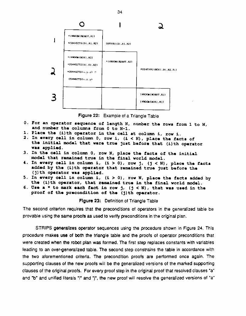
34

o '1 KRO<II (~BOT • R II

·CONNECTS(OI.RI.R21 GOTliRU (01 .RI. R2)

·INAOOII(BOXl.R2)

'1 KRO<II(~BOT. R2) ·CO~LCTS(OI.Rl.R2)

PUSIfTHRU(IlOXl.Ol.R2 .Rl) ·CONNECTS{x.y.z) :'

COHllECTS(x.z.yl

3 lHR~(~BOT.Rll

1~(BOx\.Rll

Figure 22: Example of a Triangle Table

O. For an operator .equence of length N, number the rows from 1 to N, and number the column. from 0 to N-1.

1. Place the (i)th operator in the cell at column i, row i. 2. In every cell in column 0, row i, (i < N), place the fact. of

the initial model that were true just before that (i)th operator was applied.

3. In the cell in column 0, row H, place the fact. of the initial model that remained true in the final world model.

4. In every cell in column i, (i > 0), row j, (j < N), place the fact. added by the (i)th operator that remained true just before the (j)th operator was applied.

5. In every cell in column i, (i > 0), row N, place the fact. added by the (i)th operator, that remained true in the final world model.

6. Ose a * to mark each fact in row j, (j < H), that was u.ed in the proof of the precondition of the (j)th operator.

F1gure 23: Definition of Triangle Table

The second criterion requires that the preconditions of operators in the generalized table be

provable using the same proofs as used to verify preconditions in the original plan.

STRIPS generalizes operator sequences using the procedure shown in Figure 24. This

procedure makes use of both the triangle table and the proofs of operator preconditions that

were created when the robot plan was formed. The first step replaces constants with variables

leading to an over-generalized table. The second step constrains the table in accordance with

the two aforementioned criteria. The precondition proofs are performed once again. The

supporting clauses of the new proofs will be the generalized versions of the marked supporting

clauses of the original proofs. For every proof step in the original proof that resolved clauses "a"

and "b" and unified literals "i" and "r, the new proof will resolve the generalized versions of "a"

35

and "b" and will unify the generalized versions of "i" and "j". This technique is similar to the

EGGS procedure described above inasmuch as they both require that the same objects be

unified in the generalized proof as in the original proof.

1. "Li~t It the triangle table. a. Replace each distinct constant in column zero with a distinct

variable. b. Replace each clause in columns 1 - N with the corresponding

clause ~rom the add list o~ the corresponding uninstantiated operator.

c. Rename variables so that clauses from distinct operator applications have variables with distinct names.

2. Rerun proo~s o~ preconditions usinq isomorphic ~ges o~ origina1 proo~s.

a. Each proo~ will be supported by the generalized versions o~ clauses that were marked in the oriqina1 table.

b. Each proo~ step per~orma resolution on pairs o~ clauses and uni~ication on pairs o~ literals corresponding to the pairs matched in corresponding step o~ the original proo~.

c. Substitutions generated during unification are applied throughout the entire table.

Figure 24: STRIPS Generalization Procedure

When the STRIPS generalization procedure is used to process the triangle table of Figure

22, it produces the generalized table shown in Figure 25, taken from [Fikes et al. 72]. Several

interesting generalizations have been made. The object to be moved from one room to another

has been generalized from a BOX to any object. Although the initial and final rooms were

identical in the original plan. the room variables are distinct in the generalized plan. STRIPS

has also generalized the conditions of applicability of the operator sequence. The marked

clauses in the leftmost column of the generalized table indicate the generalized conditions under

which the sequence is applicable. Initially. STRIPS only knows that the sequence applies to the

initial world model shown in Figure 20. After generalizing the triangle table, STRIPS knows the

sequence is applicable whenever the conditions in the leftmost column of the generalized table

in Figure 25 are met.

An obvious next step would be to create a new STRIPS operator representing the entire

generalized operator sequence. The new operator would have the same effect in a Single step

as the entire sequence of operators used in the original plan. The marked clauses in the

leftmost column of the table would constitute the preconditions of the new operator. The clauses

in columns 1 through N - 1 of the Nth row will constitute the add list of the operator. The delete

list could be formed by combining the instantiated delete lists from all the operators in the

36

o ·IHROOM(ROBOT.p2l

J 'COIOlICTS (pJ • p2 • pSl GOTliRU(pJ .p2 .p5l

'1 HROOII (pO. p5l

·CONNECTS(pH.p9.p5l • I NROOM(ROBOT.pSl

·COHHECTS(x.y.zl ~ PUSHTHRU(p6.p8.p5.p

CON~U:TS(,. z. yl

1 NROOW (ROBOT. p9l

INROOM(pO.p9l :3

Figure 25: Generalized Triangle Table

original sequence. STRIPS does not actually build such a macro operator. STRIPS keeps the

generalized triangle table in the form shown in Figure 25 instead. This means that the

MACROP cannot be applied in a single step in the course of solving a new planning problem.

The operators must be applied one by one. Nevertheless the table does directly indicate when

an entire sequence will be applicable to a problem situation.

There are a several reasons for preserving the generalized table. The generalized

triangle table helps STRIPS to determine when any subsequence of the original operator

sequence will be useful in a planning problem [Fikes et al. 72]. The table also appears to

contain information that would directly enable determining when the operators of a sequence

can be reordered, contrary to DeJong's comment in [Dejong and Mooney 86]. An ordering

relation can be defined so that operator A precedes operator B if there is a marked clause in the

cell at column A, row B. Any topological sort on this relation would yield a valid operator

sequence.

STRIPS has been described above in terms of "generalization" and "chunking". It can

also be viewed In terms of reformulating non-operational concept descriptions. (See Figure 3.)

Given an operator sequence OP1 ... 0PN, STRIPS contains all the information needed to

determine the condition of applicability of the entire sequence. The information is only present

implicitly, embedded in the definitions of the individual operators. One could view the sequence

description "OP1...0PW as a non-operational description of the condition of application.

STRIPS creates an operational description by building the generalized triangle table. The

marked dauses in the leftmost column constitute such an operational description.

37

3.3.3 Similar Work

Anderson's ACT· system is similar to the chunking systems described here [Anderson

83a; Anderson 83b; Anderson 86]. The ACT* system uses a learning mechanism called

Hknowledge compilation", which is based on collapsing sequences of production rules into single

rules. Each single rule has the same effect as the original sequence from which it was compiled.

Anderson describes his ACT· system as a general architecture that underlies all types of human cognition.

Many people have investigated methods of forming macro operators outside the context

of explanation-based learning. Cheng and Carbonell are working on methods of building macros

with conditional and iterative constructs [Cheng and Carbonell 86]. Korf developed a method for

finding useful macro operators that applies to any problem exhibiting a property called "serial

decomposability" [Korf 85]. The REFLECT system of Dawson and SikJossy also has a

mechanism for creating macro operators [Dawson and Siklossy 77].

3.4 EBl = Operationallzatlon

The term "operationalization" may be defined as a process of translating a "non­

operational" expression into an "operational" one. The initial expression might represent a

piece of advice, as in Mostow's FOO and BAR programs [Mostow 81; Mostow 83a], or it might

represent a concept, as in Keller's lEX COP program [Keller 83]. The initial expression is said

to be "non-operational with respect to an agent" because it is not expressed in terms of data

and actions available to the agent [Mostow 83a]. An operationalizing program faces the task of

reformulating the original expression in terms of data and actions that are available to the agent.

As shown in Figure 3, operationalization can be placed into rough correspondence with

the EBl generalization processes described previously. The explanation rules used in systems

like GENESIS or lEX-II may be viewed as non-operational specifications of the concepts that

these systems learn. The rules "specify" the concepts because they contain all the information

needed to construct the learned concepts. The concept specifications are "non-operational"

because the rules only impliCitly contain the information. The EBl techniques of GENESIS and

lEX-II serve the purpose of making the concepts explicit. Building and analyzing an explanation

is similar to the process of translating a non-operational concept into operational form. The

translation may be sald to "explain- how the operational concept description meets the

conditions given by the non-operational concept description.

,6.: •

38

3.4.1 Mostow's FOO and BAR Programs

The FOO and BAR programs were developed by Mostow to investigate the problem of

operationalizing "advice". The older FOO program is described in [Mostow 81] and [Mostow

83b]. BAR was developed as an extension to FOa and is described in [Mostow 83a] and

[Mostow 83c]. The programs were tested mainly in the domain of the card game "heartsM.

Some additional tests were run in the domain of music composition.

As an example of a non-operational expression from the hearts domain, consider the

advice to Mavoid taking pointsM .16 This advice is considered Mnon-operationalM because it is not

written in terms of actions that a player can perform. The rules of the game do not allow one to

refuse to take up the cards at the end of a trick merely because they include point cards. The

only actions available to a player are to choose to play one of the cards from his hand. As

another example, consider the advice Mdon't lead a card of a suit in which an opponent is

void"17. This advice is not operational because it requires knowing one's opponents' cards. This

data is not usually available to a player. Mostow's program can translate the advice to "avoid

taking points· into an operational form. After translation, the advice becomes Mplay a low cardM.

In this new form, the advice does directly specify an action available to the player and is

therefore considered to be operational.

In order to reformulate a piece of advice, Mostow's programs make use of several types

of knowledge. One part of the knowledge base contains a set of domain-independent Mproblem

transformation rules". Each rule has an ac~on component specifying how to rewrite an

expression representing some advice as well as conditions governing the applicability of the

rule. Examples of such rules are shown in Figure 26, taken from [Mostow 83b]. The

transformation rules are progressively applied to the initial advice, gradually changing it into a

form that meets the requirements of operationality. The knowledge base also contains domain­

dependent "concept definitions" like those shown in Figure 27, taken from [Mostow 83b].

The FOO and BAR programs differ in the type of control structure used to choose a

sequence of rule applications. FOO relies on a human user to pick an appropriate sequence of

transformation rules [Mostow 83b]. BAR uses means-ends analysis to guide the choice of

which rule to apply [Mostow 83a]. The rule sequences can be quite long, amounting to over 100

16The phrase 'aking points" means winning tricks that contain point cards. In the version of the game described previously, point cards are hearts.

17 A player is said to be "void' in suit if he does not have any cards of that suit in his hand

39

Un~olding concept de~initions: I~ F i. a concept de~ined as (lambda (xl ... xN) e), then replace the expression (F el ... eN) with the result o~ substituting el ... eN ~or xl ... xN throughout e.

Approximation ot a predicate (1): Given an expression ot the form ( .... (P S) ... ), where P is a predicate, replace the expression (P S) with the expression (High (Probability (P S»).

Approximation ot a predicate (2): Given an expression ot the form ( .... (P S) ... ), where P i. a predicate, replace (P S) with (Possible (P S», where (Possible (P S» is true unless (P S) is known to be ~a1se.

Figure 26: Problem Transformation Rules

POINT-CARDS = (LAMBDA () (SET-OF C (CARDS) (BAS-POINTS C»)

VOID = (LAMBDA (P SUIT) (NOT (EXISTS C (CARDS-IN-HAND P)

(IN-SUIT C SUIT»»

AVOID 3 (LAMBDA (E S) (ACHIEVE (NOT (DURING S E»»

'!'RI Clt :. (LAMBDA ( ) (SCENARIO (EACH P (PLAYERS) (PLAY-CARD P»

(TAKE-TRICK ('!'RIClt-WINNER»»

Figure 27: Concept Definitions

rule applications in some cases. Even the BAR program is unable to work without some human

guidance.

In order to guide the search process, BAR needs to know which specific parts of an

expression are not operational. This is done by annotating each "domain concepr with

information that indicates the operationality of the concept [Mostow 83a). For example, the

concept ·point-cards" is marked as being operational since a player always knows which cards

are worth points. The "void" predicate is not operational, since a player cannot generally know

when an opponent is void in a suit. In general, predicates can be "evaluable" or "not evaluable";

functions can be "computable" or ·not computable"; events can be "controllable" or "not

controllable·; and constraints are "achievable" or "not achievable". BAR also contains some

general knowledge about operationality. For example, there is a rule stating that "A computable

function of evaluable arguments is itself evaluable". Another rule says that "An evaluable

constraint on a controllable variable is achievable·. This knowledge can be used to guide the

search process by determining which parts of an expression are non-operational and need to be

transformed.

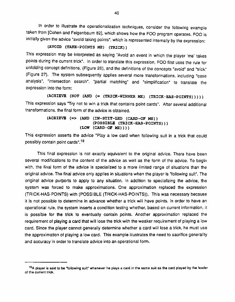
40

In order to illustrate the ope rationalization techniques, consider the following example

taken from [Cohen and Feigenbaum 82], which shows how the FOO program operates. FOO is

initially given the advice ·avoid taking points·, which is represented internally by the expression:

(AVOID (TAKE-POINTS ME) (TRICK»

This expression may be interpreted as saying "Avoid an event in which the player 'me' takes

points during the current trick". In order to translate this expression, FOO first uses the rule for

unfolding concept definitions, (Figure 26), and the definitions of the concepts "avoid" and "trick"

(Figure 27). The system subsequently applies several more transformations, including "case

analYSis", "intersection search", "partial matching" and "simplification" to translate the expression into the form:

(ACHIEVE (NOT (AND (= (TRICK-WINNER ME) (TRICK-HAS-POINTS»»)

This expression says "Try not to win a trick that contains point cards". After several additional

transformations, the final form of the advice is obtained.

(ACHIEVE (=> (AND (IN-SOIT-LED (CARD-OF ME» (POSSIBLB (TRICK-HAS-POINTS»)

(LOW (CARD-OF ME»»

This expression asserts the advice "Playa low card when following suit in a trick that could

possibly contain point cards" .18

This final expression is not exactly equivalent to the original advice. There have been

several modifications to the content of the advice as well as the form of the advice. To begin

with, the final form of the advice is specialized to a more limited range of situations than the

original advice. The final advice only applies in situations when the player is "following suit". The

original advice purports to apply to any situation. In addition to specializing the advice, the

system was forced to make approximations. One approximation replaced the expression

(TRICK-HAS-POINTS) with (POSSIBLE (TRICK-HAS-POINTS)). This was necessary because

it is not possible to determine in advance whether a trick will have points. In order to have an

operational rule, the system inserts a condition testing whether, based on current information, it

is possible for the trick to eventually contain points. Another approximation replaced the

requirement of playing a card that will lose the trick with the weaker requirement of playing a low

card. Since the player cannot generally determine whether a card will lose a trick, he must use

the approximation of playing a low card. This example illustrates the need to sacrifice generality

and accuracy in order to translate advice into an operational form.

18A player is said to be "following suit" whenever he plays a card in the same suit as the card played by the leader of the current trid(.

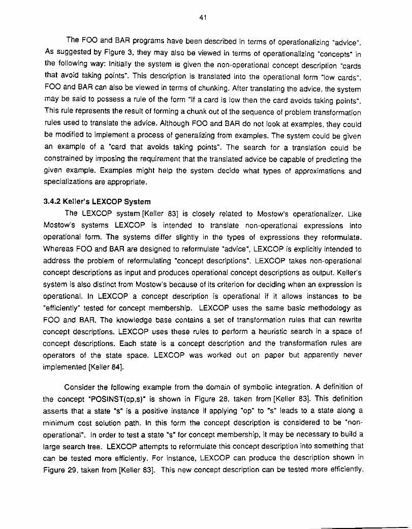
41

The FOO and BAR programs have been described in terms of operationalizing "advice".

As suggested by Figure 3, they may also be viewed in terms of operationalizing "concepts" in

the following way: Initially the system is given the non-operational concept description "cards

that avoid taking pOints". This description is translated into the operational form "low cards".

Faa and BAR can also be viewed in terms of chunking. After translating the advice, the system

may be said to possess a rule of the form "If a card is low then the card avoids taking points".

This rule represents the result of forming a chunk out of the sequence of problem transformation

rules used to translate the advice. Although FOO and BAR do not look at examples, they could

be modified to implement a process of generalizing from examples. The system could be given

an example of a "card that avoids taking points". The search for a translation could be

constrained by imposing the requirement that the translated advice be capable of predicting the

given example. Examples might help the system decide what types of approximations and

specializations are appropriate.

3.4.2 Keller's LEXCOP System

The LEXCOP system [Keller 83] is closely related to Mostow's operationalizer. Uke

Mostow's systems LEXCOP is intended to translate non-operational expressions into

operational form. The systems differ slightly in the types of expressions they reformulate.

Whereas FOO and BAR are designed to reformulate "advice", LEXCOP is explicitly intended to

address the problem of reformulating "concept descriptions". LEXCOP takes non-operational

concept descriptions as input and produces operational concept descriptions as output. Keller's

system is also distinct from Mostow's because of its criterion for deciding when an expression is

operational. In LEXCOP a concept description is operational if it allows instances to be

"efficiently" tested for concept membership. LEXCOP uses the same basic methodology as

FOO and BAR. The knowledge base contains a set of transformation rules that can rewrite

concept descriptions. LEXCOP uses these rules to perform a heuristic search in a space of

concept descriptions. Each state is a concept description and the transformation rules are

operators of the state space. LEXCOP was worked out on paper but apparently never

implemented [Keller 84].

Consider the following example from the domain of symbolic integration. A definition of

the concept "POSINST(op,s)" is shown in Figure 28, taken from [Keller 83]. This definition

asserts that a state "s" is a positive instance if applying MOp" to "s" leads to a state along a

minimum cost solution path. In this form the concept description is considered to be "non­

operational". In order to test a state MS· for concept membership, it may be necessary to build a

large search tree. LEXCOP attempts to reformulate this concept description into something that

can be tested more efficiently. For instance, LEXCOP can produce the description shown in

Figure 29, taken from [Keller 83]. This new concept description can be tested more efficiently,

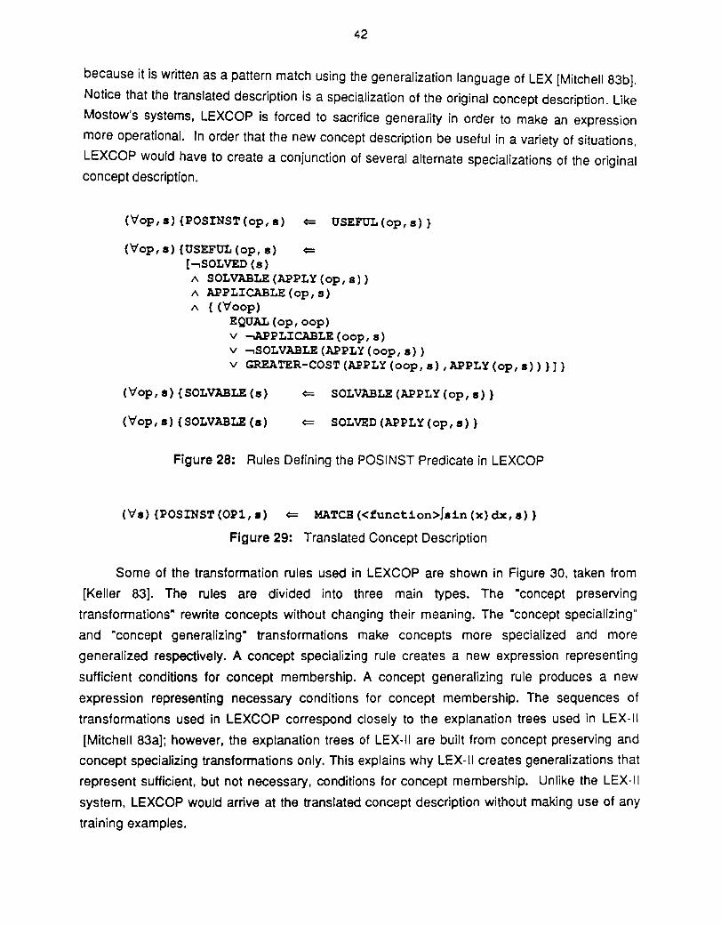
42

because it is written as a pattern match using the generalization language of LEX [Mitchell 83b].

Notice that the translated description is a specialization of the original concept description. Like

Mostow's systems, LEXCOP is forced to sacrifice generality in order to make an expression

more operational. In order that the new concept description be useful in a variety of situations,

LEXCOP would have to create a conjunction of several alternate specializations of the original concept description.

(~op,a){POSINST(op,a) <= OSEFUL(op,s)}

(~op,a){OSEFOL(op,a) <= [-.SOLVED (a)

A SOLVABLE(APPLY(op,s) A APPLlCABLE(op,s) A {(~oop)

EQOAL (op, oop) v -.APPLlCABLE(oop,s) v -.SOLVABLE(APPLY(oop,a» v GREATER-COST(APPLY(oop,a},APPLY(op,a»}]}

(~op,a){SOLVABLE(a) <= SOLVABLE (APPLY (op, a) }

(~op,a){SOLVABLE(a) <= SOLVED(APPLY(op,a}}

Figure 28: Rules Defining the POSINST Predicate in LEXCOP

(~a}{POSINST(OP1,.) <= MATCB«function>fain(x}dx,a)}

Figure 29: Translated Concept Description

Some of the transformation rules used in LEXCOP are shown in Figure 30, taken from

[Keller 83]. The rules are divided into three main types. The ·concept preserving

transformations· rewrite concepts without changing their meaning. The ·concept specializing"

and "concept generalizing" transformations make concepts more specialized and more

generalized respectively. A concept specializing rule creates a new expression representing

sufficient conditions for concept membership. A concept generalizing rule produces a new

expression representing necessary conditions for concept membership. The sequences of

transformations used in LEXCOP correspond closely to the explanation trees used in LEX-II

[Mitchell 83a]; however, the explanation trees of LEX-II are built from concept preserving and

concept specializing transformations only. This explains why LEX-II creates generalizations that

represent sufficient, but not necessary, conditions for concept membership. Unlike the LEX-II

system, LEXCOP would arrive at the translated concept description without making use of any

training examples.

43

concept Preserving Transforms: 1. Expand definition of a predicate. 2. Constraint Back-Propagation. 3. Enumerate the values of a universal variable.

Concept Specializing Transforms: 1. Add a conjunct to an expression. 2. Delete a disjunct from an expression. 3. Instantiate a universal variable.

Concept Generalizing Transforms: 1. Add a disjunct to an expression. 2. Delete a conjunct from an expression.

Figure 30: Transformation Rules in LEXCOP

Keller has proposed a new system called METALEX, which is intended to build on the

ideas of LEXCOP [Keller 84]. METALEX is intended to show how learning systems can exploit

explicit representations of contextual knowledge, i.e., knowledge of the context in which

learning takes place. Keller defines "contextual knowledge" to have several components,

including knowledge of the task the system is intended to perform and knowledge of the

algorithm used by the system's performance element. Keller argues that contextual knowledge

is useful for several purposes. For example, he suggests that a learning system can utilize

contextual knowledge to automatically formulate its own learning tasks. By analyzing the

algorithm used by the performance element, a learning system can formulate a performance

improvement plan. The improvement plan might involve modifying the algorithm to insert a

concept membership test at some location. The plan would initially describe the concept in non­

operational terms. The learning element would then be faced with the task of translating the

concept into an operational form. This process suggests a solution to the "wandering

bottleneck" problem. Contextual knowledge gives a learning system the potential ability to

handle this problem by formulating new learning tasks to attack bottlenecks as they move

around in the performance element of a system.

MET ALEX is intended to use a complex notion of "ope rationality" . Faa, BAR and

LEX COP all use a simple notion of "ope rationality" . Expressions and terms are either

completely operational or completely non-operational. METALEX is based on the view that the

operationality of an expression is often a matter of degree. This is especially true when

operationality is defined in terms of the efficiency of testing concept membership. Efficiency is

naturally measured in terms of continuous variables like time or space complexity. METALEX

attempts to use such continuous measures of operationality.

44

Unlike FOO, BAR and LEXCOP, the proposed METALEX system would make use of

empirical information. Keller proposes that METALEX should collect data indicating the CPU

time expended in evaluating each part of a concept description. This data can be used to

determine which part of an expression is the least operational and most in need of

reformulation. The empirical information would help guide the process of searching in the space

of concept descriptions. Keller also proposes to collect data to help determine when a concept

can be safely approximated. In particular, the proposed system would run empirical tests to

determine how often an approximate concept description would make errors of inclusion or

exclusion. The results could justify the use of an approximate concept description, if the

approximation leads to few errors in practice.

3.4.3 Similar Work

Techniques for operationalization have not been studied extensively in the field of

machine learning. Some automatic programming methods can be viewed in terms of

operationalization. The transformational implementation methodology developed by Balzer is a

case in point [Balzer et al. 76). This technique takes a (non-operational) program specification

as input. A series of correctness preserving transformations are then applied to the

specification, gradually refining it into an executable (operational) program. This method has

been used by Swartout to build knowledge-based expert systems for which human oriented

explanations can easily be generated [Swartout 83).

3.5 ESl = Justified Analogy This section will discuss techniques for performing "justified" analogical reasoning.

Traditional methods of reasoning by analogy require making a guess about what information

should be transferred from a remembered analogous situation to a new situation. The "justified"

version of analogy tries to avoid guessing. One approach to justified analogy involves mapping

sequences of "inference rules", or "explanations", from analogues to target examples. The

inference rules might encode "causal relations" as in [Winston et al. 83; Kedar-Cabelli 85;

Gentner 83) or they might represent problem-solving "derivation" steps as in [Carbonell 86).

(See Figure 3.) Since the inference rules contain their conditions of applicability, the system

needs only to verify that the mapped rules apply to the new situation in order to avoid making

guesses. This suggests that explanation-based analogy (EBA) would be a reasonable name

for these these techniques.

45

3.5.1 Winston's ANALOGY Program

Winston and his coworkers have developed the ANALOGY system [Winston et al. 83].

This program is intended to learn "physical" or "structural" descriptions of objects. The program

is given "functional definitions· of objects as input. By finding analogies between ·precedents"

and "practice examples", ANALOGY transforms the functional definition into a physical or

structural description.

The ANALOGY program wili be described using the example of a drinking cup. The input

to the system is a functional definition of a cup, shown in Figure 31, taken from [Winston et al.

83). This definition gives three conditions that must be met in order that an object function as a

drinking cup. The object must be a "stable, liftable, open vessel". These conditions are

considered to be functional specifications but not physical or structural properties. ~ variety of

physically different objects could fulfill these three functional criteria. In addition to a functional

definition, the system is also given an example of a cup, shown in Figure 32, taken from

[Winston et ai. 83]. ANALOGY is also provided with a set of precedents that are used to

reason by analogy. These precedents include descriptions of objects, like bricks, suitcases and

bowls, that are useful for establishing the connection between physical properties and functional

specificatio"ns.

FIgure 31: Functional Definition of a Cup

ANALOGY begins by trying to confirm that the example is indeed a cup. The functional

definition network Is retrieved and superimposed on the example network. Next the system tries

to establish each of the three criteria in the definition, I.e., the program must show that the

example is a -stable, liftable, open vesse'-. Each condition can be established either by

verifying that the condition appears directly In the description of the example or by reasoning

from a precedent. The suitcase precedent is used to show that the example is liftable. The

description of the suitcase precedent contains a causal chain. This chain has two steps

asserting that (1) 'he suitcase is liftable because it is light and graspable- and (2) "the suitcase

46

___ 1=5_ "Shl

Figure 32: Example of a Cup

is graspable because it has a handle-. In order to use the chain, ANALOGY determines a

correspondence between parts of the cup example and parts of the suitcase precedent, using a

method called -importance dominated matching- [Winston 82]. While transferring the chain, the

program tests whether the antecedents of the chain are found in the example. In this case the

cup example does in fact contain the -light- and "handle- relations. This means the condition of

being -liftable- is successfully established. In a similar manner, ANALOGY uses the brick

precedent to show that the example is stable and the bowl precedent to show that the example

is an open vessel. The final version of the example network is shown in Figure 33, taken from

[Winston et aI. 83]. This diagram shows all the causal chains transferred from the precedents

to the cup example.

After establishing the example to be a cup, ANALOGY creates a general rule. The rule is

intended to summarize the set of physical properties that enabled the example to function as a

cup. An English paraphrase of the new rule is shown in Figure 34. The "IF- part of this rule was

built from the antecedents of the causal chains transferred from precedents. The -rHEW part

asserts an object to be a cup. The -UNLESS- conditions correspond to the intermediate nodes

of the transferred causal chains. These conditions are included because the causal connections

are not considered to be infallible. For example, the causal link asserting that "an object is

graspable if it has a handle- might be wrong in some cases. By adding the -UNLESS- condition.

the rule is understood to mean -an object is graspable if it has a handle, unless there is some

reason to believe otherwise-.

47

cup

.-----\ ~--, I ~-\ I I

: I I I I I ako

- - ,- ,. - - ~ open-vessel ~/:r __ --',"" ..... I I is ~~

" ..... 1- --"7 ~ stable' \ '- '5 ~ \

- - - .:. ~ liftable "

++,\ \~ I I \, 'I 1, 1 I

~ has; f 1/' I I ./ I I

_ ...... -:,. ..... /1 I ...- '" ;1/

;' -- " f\ l ,I I is rgh 1/, / ~/ aka 1 t ////

Q _ ~ .handle:., ~ / / /

aka .... -: - - - -:.. --' / / i = · bonom / / 5 / ~ / /

Q . fiat II

_ aka '/ . • body ............. 1.S '" ;

Q _ --~ ~_aJl- -_-- ..-

ako ..... ..,.. - - - - --- - -, ~ concavlt}'

15 ~ upward-pOinting

Figure 33: Final Version of Example Network

Ii' : AN OBJECT IS LIGHT AND BAS A HANDLE, A FLAT BOT'1'OM AND AN UPWARD POINTING CONCAVITY,

THEN: THE OBomCT IS A CUP,

UNLESS: Tim OBomCT IS NO'1' ST.AB.LK, OR NOT LIFTABLE, OR NO'1' AN OPEN VESSEL, OR NOT GRASP.AB.LK.

FJgure 34: Rule Extracted From Network

A question arises regarding whether the precedents are really necessary in the

ANALOGY system. According to Winston, "The precedents are essential for otherwise there

would be no way to know which aspects of the example are relevant" [Winston et al. 83], (page

433). The precedents might appear to be necessary because they contain causal information in

the form of links between causes and effects, ANALOGY may be said to possess an

"extensional theorY of causes and effects In the form of precedents. This can be contrasted

with an "intensional theory" In the form of general rules connecting causes and effects [Mitchell

et al. 86]. Nevertheless, Winston's data base of precedents is really an intensional theory in

disguise. ANALOGY has the ability to extract causal relations from precedents and transfer

them to new situations. This implies it can determine which conditions must hold for a causal

link to be in effect. As observed by Mitchell, the ANALOGY program implicitly assumes a

causal link such as "FEATURE1 (A) -. FEATURE2(A)" is supported by a general rule of the

48

form "(V'x){FEATURE1 (x) ~ FEATURE2(x)}" [Mitchell et al. 86]. If data base of rules were

created by extracting causal links from the precedents, the result would be a program looking

more like GENESIS or LEX-II. There may be a reason for storing causal rules in the context of

precedents. The causal rules may be faulty. When contradicted by future information, they will

need revision. The precedents might help determine how to revise faulty rules.

Winston's ANALOGY program can also be viewed in terms of generalization, chunking

and operationalization. (See Figure 3.) The rule in Figure 34 can be taken as a generalization

of the single example of a cup that was provided to the system. The rule may also be seen as

an operationalization of the functional definition of a cup. The original definition of a cup in

Figure 31 in may be considered to be "non-operational", because it describes a cup in functional

terms. The final rule in Figure 34 is operational because it describes cups in physical or

structural terms. Winston's program also performs chunking. Three causal chains are taken

from three precedents, the suitcase, the brick and the bowl, and are spliced together to build an

explanation of the cup example. The explanation is then collapsed into a single rule

representing a chunk.

3.5.2 Carbonell's Derivational Analogy Method

Derivational Analogy (DA) was developed by Carbonell to investigate analogical

reasoning in the context of problem solving [Carbonell 86; Carbonell 83a]. The DA technique

solves a new problem by making use of a solution derivation that was generated while solving a

previous problem. The new problem is solved by recreating sequences of decisions and

justifications for decisions that were used to solve a precedent problem. Carbonell uses

derivations in a way similar to the manner in which Winston uses causal networks. Carbonell

proposes transferring derivations between examples, whereas Winston proposes transferring

causal networks. Derivations and causal networks are both types of dependencies or

justifications. Inasmuch as DA involves transferring justifications from a precedent to a new

situation, it may be seen as a type of justified analogical reasoning.

The DA method was originally developed to remedy a limitation of earlier work on analogy

in problem solving. Carbonell's earlier work involved solving new problems by directly modifying

solutions to previously solved problems [Carbonell 83b]. For example, one might try to write a

sorting program by directly modifying the code used in a previous sorting program. The difficulty

can be illustrated by considering the following problem from [Carbonell 86]. Suppose one

wanted to write a LISP sorting program, and one had already written a PASCAL program

implementing quicksort. The approach of directly modifying the PASCAL program would either

fail completely or lead to a poor LISP program. This would happen because a good LISP

implementation of quicksort would look quite diHerent from the PASCAL program due to

49

differences in the structures of these languages. Nevertheless, the LISP and PASCAL programs

might share the same underlying design strategy. They could both use a divide and conquer

approach manifested in terms of partitioning sets. This strategic information is ignored by an

analogy process that directly transforms the code of one program into the code of another. DA

avoids this problem since it does not try to directly transform one solution into another. The DA

method transfers information at the level of "derivations" rather than "solutions". DA would

solve the sorting problem by transforming the derivation of the PASCAL program into a

derivation of a LISP program.

Carbonell gives a detailed specification of the sorts of information that should be

contained in a derivation [Carbonell 86; Carbonell 83a]. A derivation is supposed to include the

"hierarchical goal structure" used to generate the solution. The goal structure is represented in

terms of the ·sequence of decisions" made while solving a problem. For each decision, the

derivation should list the alternative that was chosen as well as those that were considered, but

not chosen. The record of a decision should include the reasons for the decision, (Le., the

derivation might record an explanation of the decision along with dependency links to aspects of

the problem specification and dependency links to general knowledge). The derivation should

also indicate how each decision depends on prior decisions and influences subsequent

decisions. Finally, the derivation should record the initial segments of any dead end paths were

explored, along with reasons that paths appeared promising and reasons the paths ultimately

failed.

In order to use the DA method to solve a problem, it is necessary to find prior problem

situations that are analogous to the current situation. The DA system begins by solving a

problem using general techniques. e.g., application of weak methods or instantiating a general

problem solving schema like divide and conquer [Carbonell 86]. A trace is maintained to record

these initial stages of the problem solving process. Appropriate analogous problems are found

by matching the initial analysis trace of the current problem with the initial analysis of previous

problems. This seems to beg the question since one is tempted to ask what makes two initial

analysis traces similar.

After finding an analogous problem, the derivation of the analogous problem's solution is

retrieved and applied to the new situation. A derivation may be transferred to a new problem in

the following way. The system must follow the sequence of decisions in the derivation and

reconsider each one in the context of the current problem. In order to reconsider each decision,

the system must examine the reasons for the decision. This can be done by examining the

dependency links to the previous problem situation and to general knowledge. If the relevant

aspects of the problem specification are the same and the general knowledge applies to the

50

new situation, then the same decision can be made. Otherwise, the system must reconsider the

decision. Carbonell actually provides a more detailed description of how to transfer a derivation

from one problem to another [Carbonell 86].

3.5.3 Analogy versus Generalization

The explanation-based versions of analogy and generalization differ mainly on the issue

of schema formation. Systems like GENESIS and SOAR are naturally viewed as generalizers

because they convert explanations (operator sequences) into schemata (chunks). The

schemata represent compiled versions of the explanations that need only be instantiated to

apply to new problems. The process of schema instantiation solves a new problem in a single

step, bypassing all the intermediate steps of the explanation. In contrast to this, Carbonell's DA

method is more naturally viewed in terms of analogy because it does not convert an-explanation

(derivation) into a schema. but rather keeps the explanation in its original form. In order to solve

a new problem, DA must pass through all the steps in the original explanation, possibly

modifying the explanation to some degree.

The schema-building approach seems to provide some efficiency advantages. Schema­

building systems can usually solve new problems faster since they omit all the intermediate

steps of the derivation, although the process of instantiating a schema may be slower, in some

situations, than replaying the original derivation. The schema approach suffers from the

disadvantage that a schema is not immediately useful if a new problem falls outside its scope.

The DA method does not suffer from this problem. If one assumes that the DA method can

modify an explanation so it can apply to a new problem, then the original explanation does not

have a fixed range of application.

In order to decide which approach is better for a given application, it is necessary to

recognize that there are really two issues here:

• Should a schema be formed from the explanation?

• Should the original explanation be retained?

A reasonable compromise would involve answering "yes" to both of these questions.

Explanations can be converted into schemata and also kept around in original form or in

generalized form.19 A new problem can be processed by first trying to instantiate a schema. If

that fails, the problem may be processed by modifying an explanation using the DA method.

19GENESIS and STRIPS take such intermediate approaches. GENESIS builds a schema also keeps the generalized explanation. STRIPS generalizes the explanation (i.e .• the triangle table) but does not form a schema represanting the entire generalized explanation as a single operator.

51

3.5.4 Similar Work

The EBA methods discussed in this section are similar to other recent research in

analogical reasoning. In particular, they are related to Gentner's "structure mapping" theory of

analogy [Gentner 83]. This theory involves using a principle called "systematicity" to determine

what information should be mapped from the analogue to the target example. According to the

systematicity principle, analogy processes should transfer "systems of relations". A system of

relations involves "first order" relations that are governed by "higher order" relations. Causal

relations are one type of higher order relation. The systematicity criterion often leads to

transferring networks of causal relations from one example to another. The causal nets can be

interpreted as explanations. For this reason the systematicity principle often results in

transferring explanations from the analogue to the target, just as in explanation-based analogy.

Another method of justified analogical reasoning, called "Purpose-Directed Analogy",

(PDA), has been proposed in [Kedar-Cabelli 85]. PDA is intended to address the question of

deciding which causal network should be transferred from the analogue to the target, in cases

when the analogue contains many possible causal networks. Kedar-Cabelli argues that the

methods of Winston and Gentner are not able to operate unless the relevant network is

specified in advance. PDA tries to avoid this limitation by using the "purpose of the analogy" to

select the relevant network from among many.

A technique similar to derivational analogy has been used by Mitchell and coworkers in

the domain of logic circuit design [Mitchell et al. 83). Their REDESIGN system serves as an

assistant to a human for the purpose of designing new circuits by analogy with existing ones.

REDESIGN combines causal reasoning about circuit behavior with knowledge about the design

plan of the original circuit in order to focus attention on the parts that must be modified. Mostow

has investigated derivational analogy methods in the context of design problems in general,

including both circuit design and program generation [Mostow 85). He has examined some

difficulties that arise in the course of attempting to replay derivations. This study has led him to

propose criteria about the types of information that should be included in derivations.

An entirely different approach to justified analogy has been developed by Davies and

Russell [Davies and Russell 86]. Their technique involves utilizing "determinations", e.g., a rule

asserting that -the value of feature A determines the value of feature B". A system in possession

of determinations can make logically sound inferences from precedents to new examples. Other

knowledge-intensive approaches to analogical reasoning include [Burstein 86; Hall 85].

52

3.6 Additional Related ESl Research

Several additional research projects are related to explanation-based learning but do not

fit neatly into any of the categories. Silver and Schank fall into this group. Silver has built a

program called LP, which learns heuristics for solving algebraic equations. lP uses an analytical

learning technique called "precondition analysis" (PA) [Silver 86]. The PA method is used to

infer the strategic purpose of an operator, when the lP system sees it used within a sequence

of operators. Suppose the two operators, P(i) and P(i+ 1), appear within the sequence,

P(1), ... ,P(i-1),P(i),P(i+1), ... P(N). The PA method will assume that P(i) was used to achieve

some preconditions of P(i+ 1). Suppose A is a set containing all the preconditions of operator

P(i+ 1) and that B is a set containing members of A that are true before P(i) was applied. The set

difference, A - B, represents those preconditions of P(i+ 1) that were brought about by the

operator P(i). PA would then infer that these conditions are the "strategic purpose" of P(i). After

learning the purpose of an operator, lP would use the information as a search control heuristic

in future problem solving. Precondition analysis is related to EBl methods in two ways. It can

learn from a single observation of an operator sequence applied to an algebra problem. It also

relies on background knowledge about the preconditions of operators. Precondition analysis

differs somewhat from analytical techniques like constraint-back propagation (CBP) and EGGS.

PA can be applied to operators that are ill-behaved in certain ways that would cause these

methods to fail [Silver 85].

Schank and coworkers have been working on a theory of learning and memory that is

similar to EBl. Schank envisions a role for explanations in learning; however, he uses

explanations in a somewhat different way than the EBl systems described above. He has

proposed a theory called "failure driven memory" (FDM) based on the idea that learning is

possible whenever a person encounters a failure of expectations [Schank 82]. In the course of

attempting to explain the failure, a person is reminded of previous episodes that can be

understood using the same explanation. Such reminding is possible if memory is indexed in

terms of ·pattems of explanations·. Schank has proposed a typology of standard explanation

patterns [Schank 84; Schank and Riesbeck 85]. Hammond has used the FDM method in his

WOK and CHEF programs [Hammond 83; Hammond 85]. Salzberg has used FDM in his

HANDICAPPER and FORECASTER programs [Salzberg 83; Salzberg and Atkinson 83].

Schank's FDM theory can be compared to EBl in the following way: According to FDM, if

event A causes one to be reminded of event e, then A and e share a common explanation. In

the context of EBl, if A and B are instances of a single generalization, then they can both be

understood using the same explanation. Due to the emphasis that Schank places on case­

based reasoning, his work bears an especially strong resemblance to explanation-based

53

analogy.

4 Formalizations of Explanation-Based Learning

4.1 Mitchell's EBG Formalism

A formalism called explanation-based generalization (EBG) has recently been

proposed by Mitchell [Mitchell et al. 86]. EBG attempts to capture the essential elements of most

explanation-based learning systems that have been proposed. EBG is similar in spirit to Mitchell

and Utgoff's LEX-II system; however, it uses a more uniform set of methods and is cast in a

form that is more clearly applicable to other domains. Mitchell describes the EBG framework as

a "domain independent method ... for using domain dependent knowledge to guide

generalization" [Mitchell et al. 86], (page 49).

The EBG formalism consists of two parts called the "EBG Problem" and the "EBG

Method". A formal specification of the problem is shown in Figure 35. The EBG problem is

defined in terms of four parameters that are necessary for all EBG systems. The "goal concept"

represents the objective of the learning program. This parameter provides a non-operational

specification of the concept that the system will attempt to learn. In Mitchell's presentation of

EBG, the goal concept is represented as an atomic predicate calculus formula, possibly

containing free variables, e.g., POSINST(OP-3,s) or CUP(obj). The "operationality criterion"

specifies the types of concept descriptions that are considered to be operational. Mitchell

represents the criterion as a list of predicates that are observable or easily evaluable. A concept

description is considered operational if and only if it is expressed entirely in terms of predicates

from this list. The "training example" is a description of an object that is an instance of the goal

concept. The training example parameter is described in operational terms, i.e., using

predicates from the list of operational predicates. Finally, the "domain theory" parameter is a

set of rules describing the domain from which the example and goal concept are drawn. The

rules must be capable of proving that the training example meets the conditions for being an

instance of the goal concept. In Mitchell's presentation, the domain theory is represented as a

set of Horn clauses.

The EBG system is charged with the task of reformulating the goal concept into an

expression that meets the operationality criterion. The new concept description need not be

exactly equivalent to the original goal concept. so long as it is both (a) a specialization of the

goal concept and (b) a generalization of the training example. In order to create such a concept

description, the EBG system uses a two step process similar to the ones described above for

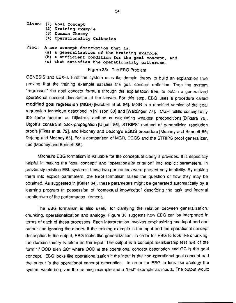
Given: (1) Goal Concept (2) Training Example (3) Domain Theory

54

(4) Operationality Criterion

Find: A new concept description that is: (a) a generalization of the training example, (b) a sufficient condition for the goal concept, and (c) that satisfies the operationality criterion.

Figure 35: The EBG Problem

GENESIS and lEX-II. First the system uses the domain theory to build an explanation tree

proving that the training example satisfies the goal concept definition. Then the system

"regresses" the goal concept formula through the explanation tree, to obtain a generalized

operational concept description at the leaves. For this step, EBG uses a procedure called

modified goal regression (MGR) [Mitchell et al. 86]. MGR is a modified version of the goal

regression technique described in [Nilsson 80] and [Waldinger 77]. MGR fulfills conceptually

the same function as Dijkstra's method of calculating weakest preconditions [Dijkstra 76],

Utgoffs constraint back-propagation [Utgoff 86), STRIPS' method of generalizing resolution

proofs [Fikes et al. 72], and Mooney and Dejong's EGGS procedure [Mooney and Bennett 86;

Dejong and Mooney 86]. For a comparison of MGR, EGGS and the STRIPS proof generalizer,

see [Mooney and Bennett 86].

Mitchell's EBG formalism is valuable for the conceptual clarity it provides. It is especially

helpful in making the ·goal concept· and ·operationality criterion· into explicit parameters. In

previously existing EBl systems, these two parameters were present only implicitly. By making

them into explicit parameters, the EBG formalism raises the question of how they may be

obtained. As suggested in [Keller 84], these parameters might be generated automatically by a

learning program in possession of ·contextual knowledge" describing the task and internal

architecture of the performance element.

The EBG formalism is also useful for clarifying the relation between generalization.

chunking, operationalization and analogy. Figure 36 suggests how EBG can be interpreted in

terms of each of these processes. Each interpretation involves emphasizing one input and one

output and ignoring the others. If the training example is the input and the operational concept

description is the output, EBG looks like generalization. In order for EBG to look like chunking.

the domain theory is taken as the input. The output is a concept membership test rule of the

form "if OCD then GC· where OCD is the operational concept description and GC is the goal

concept. EBG looks like operationalization if the input is the non-operational goal concept and

the output is the operational concept description. In order for EBG to look like analogy the

system would be given the training example and a ·tesr example as inputs. The output would

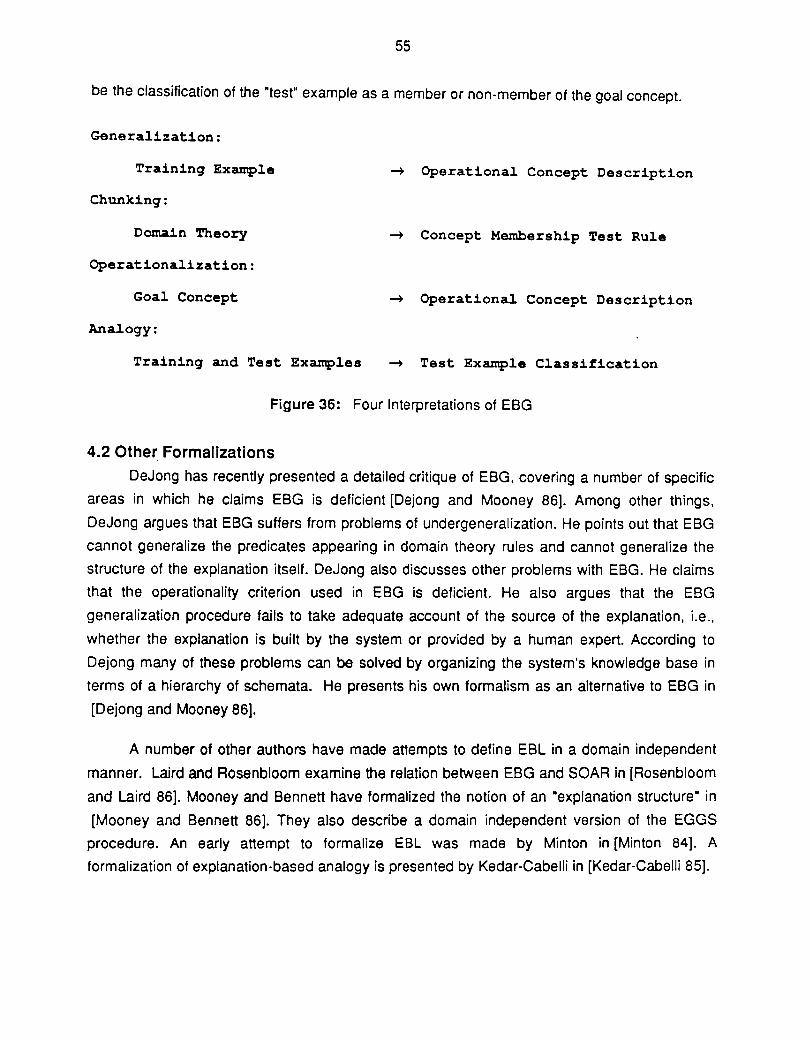
55

be the classification of the "test" example as a member or non-member of the goal concept.

Generalization:

Traininq Example ~ Operational Concept Description

Chunkinq:

Domain Theory ~ Concept Membership Test Rule

Operationalization:

Goal Concept ~ Operational Concept Description

Analoqy:

Traininq and Test Examples ~ Test Example Classi~ication

Figure 36: Four Interpretations of EBG

4.2 Other Formalizations

Dejong has recently presented a detailed critique of EBG, covering a number of specific

areas in which he claims EBG is deficient [Dejong and Mooney 86]. Among other things,

Dejong argues that EBG suffers from problems of undergeneralization. He points out that EBG

cannot generalize the predicates appearing in domain theory rules and cannot generalize the

structure of the explanation itself. Dejong also discusses other problems with EBG. He claims

that the operationality criterion used in EBG is deficient. He also argues that the EBG

generalization procedure fails to take adequate account of the source of the explanation, i.e.,

whether the explanation is built by the system or provided by a human expert. According to

Dejong many of these problems can be solved by organizing the system's knowledge base in

terms of a hierarchy of schemata. He presents his own formalism as an alternative to EBG in

[Dejong and Mooney 86].

A number of other authors have made attempts to define EBL in a domain independent

manner. Laird and Rosenbloom examine the relation between EBG and SOAR in [Rosenbloom

and Laird 86]. Mooney and Bennett have formalized the notion of an "explanation structure" in

[Mooney and Bennett 86]. They also describe a domain independent version of the EGGS

procedure. An early attempt to formalize EBL was made by Minton in [Minton 84]. A

formalization of explanation-based analogy is presented by Kedar-Cabelli in [Kedar-Cabelli 85].

56

5 An Evaluation of EBl The EBG formalism clarifies a number of outstanding issues in the field of explanation­

based learning. Mitchell's formalism draws attention to the fact that an EBG system must be

provided with a "domain theory" and a "goal concept" at the outset, before learning can occur. A

couple of questions are suggested by this fact:

• Are training examples necessary for EBG systems?

• Do EBG systems learn anything they do not already know?

The first question results from the following observation. If an EBG system possesses a

domain theory capable of explaining an example, the same theory is probably sufficient for

generating the example in the first place. If the system can generate its own example, the

training example parameter is not necessary. FOO, BAR and LEXCOP take just this approach

of reformulating a non-operational concept without making use of an example.

Mitchell's EBG method might be modified to operate without training examples. This

would require omitting the step that involves explaining how the example satisfies the goal

concept. The following "explanation step· would be used instead: The system would find any

explanation tree that has the goal concept at the root and only operational statements at the

leaves. The modified explanation process would be permitted to use any operational predicate

as an assumption in the explanation. The resulting explanation process might be more time

consuming than if an example were being explained. Some search control techniques that

would be useful in the presence of a training example would not apply to the modified

explanation process. If Mitchell's EBG method were modified in this way, the result would look

very much like Keller's LEXCOP system.

In some domains the ability to explain an example is not equivalent to the ability to

generate an example in the first place. Consider the 8-QUEENS problem as an example.

Suppose an EBG system were given the goal concept "mutually non-attacking positions of 8

queens·. Given a theory about how queens can attack, a system could easily verify that a

solution satisfies the goal concept. Nevertheless, it is much more difficult to find a solution than

to verify the correctness of a solution provided by a teacher. This argument applies to the whole

class of NP-complete problems, of which the N-QUEENS problem is an instance. The NP­

complete problems all have the property that solutions are easy to verify but difficult to find. For

such problems an example solution provided by a teacher can be very useful.

Even if an EBG system is capable in principle of reformulating goal concepts without

using examples, there would nevertheless be a useful role for examples provided by a teacher.

EBG normally does not produce an exact reformulation of a goal concept. It usually creates a