Data augmentation and feature selection for

automatic model recommendation in computational

physics

Thomas DANIEL∗†, Fabien CASENAVE∗, Nissrine AKKARI∗, David RYCKELYNCK†

January 12, 2021

Abstract

Classification algorithms have recently found applications in computational physics for the selec-tion of numerical methods or models adapted to the environment and the state of the physicalsystem. For such classification tasks, labeled training data come from numerical simulationsand generally correspond to physical fields discretized on a mesh. Three challenging difficultiesarise: the lack of training data, their high dimensionality, and the non-applicability of commondata augmentation techniques to physics data. This article introduces two algorithms to addressthese issues, one for dimensionality reduction via feature selection, and one for data augmenta-tion. These algorithms are combined with a wide variety of classifiers for their evaluation. Whencombined with a stacking ensemble made of six multilayer perceptrons and a ridge logistic re-gression, they enable reaching an accuracy of 90% on our classification problem for nonlinearstructural mechanics.Keywords: machine learning, classification, automatic model recommendation, feature selec-tion, data augmentation, numerical simulations.

1 Introduction

Classification problems can be encountered in various disciplines such as handwritten text recog-nition [1], document classification [2], and computer-aided diagnosis in the medical field [3],among many others. In numerical analysis, classification algorithms are getting more andmore attention for the selection of efficient numerical models that can predict the behaviorof a physical system with very different states or under various configurations of its environ-ment [4, 5, 6, 7, 8, 9, 10, 11]. Classifiers have been used as reduced-order model (ROM) selectorsin [4, 5, 8, 9, 11] in computational mechanics, enabling the computation of approximate solutionsat lower cost by replacing a generic high-fidelity numerical model by a specific (or local) ROMadapted to the simulation’s context. Reduced-order modeling [12, 13] consists in identifying anappropriate low-dimensional subspace on which the governing equations are projected in orderto reduce the number of degrees of freedom of the solution. In [11], the combination of a classifierwith a dictionary of local ROMs has been termed dictionary-based ROM-net. Such approachesare promising numerical methods using both physics equations and a collection of latent spacesto compute approximations of solutions lying in nonlinear manifolds.

∗ SafranTech, Rue des Jeunes Bois, Chateaufort, 78114 Magny-les-Hameaux (France).† MINES ParisTech, PSL University, Centre des materiaux (CMAT), CNRS UMR 7633, BP 87, 91003 Evry

(France).

1

arX

iv:2

101.

0453

0v1

[st

at.M

L]

12

Jan

2021

Dictionary-based ROM-nets use a physics-informed automatic data labeling procedure basedon the clustering of numerical simulations. Due to the cost of numerical simulations, trainingexamples for classification are limited in number. Moreover, the dimensionality of input datacan be very high, especially when dealing with physical fields discretized on a mesh (finite-difference methods [14], finite-element method [15], finite-volume method [16]) or with bondgraphs modeling engineering systems [17].

When classification data are high-dimensional, dimensionality reduction techniques can beapplied to reduce the amount of information to be analyzed by the classifier. For classificationproblems where the dimension of the input data is higher than the number of training examples,dimensionality reduction is crucial to avoid overfitting. In addition, when considering physicalfields discretized on a mesh, the dimension of the input space can reach 106 to 108 for industrialproblems. In such cases, the input data are too hard to manipulate, which dramatically slowsdown the training process for the classifier and thus restrains the exploration of the hyperpa-rameters space, as it requires multiple runs of the training process with different values for thehyperparameters. Applying data augmentation techniques to increase the number of examplesin the training set is also impossible, as it would cause memory problems. Therefore, dimen-sionality reduction is recommended not only for reducing the risk of overfitting, but also forfacilitating the training phase and enabling data augmentation.

Feature selection [18] aims at decreasing the number of features by selecting a subset of theoriginal features. It differs from feature extraction, where new features are created from theoriginal ones (e.g. Principal Component Analysis, PCA, and more generally encoders takenfrom undercomplete autoencoders [19]). Feature selection can be seen as applying a mask to ahigh-dimensional random vector to get a low-dimensional random vector containing the mostrelevant information. It is preferred over autoencoders when interpretability is important [20].Furthermore, contrary to undercomplete autoencoders trained with the mean squared error loss,most feature selection algorithms do not intend to find reduced features enabling the reconstruc-tion of the input: features are selected for the purpose of predicting class labels, which makesthese algorithms more goal-oriented for supervised learning tasks.

Among the existing feature selection algorithms, univariate filter methods consist in com-puting a score for each feature and ranking the features according to their scores. The scoremeasures how relevant a feature is for the prediction of the output variable. If Nf is the targetnumber of features, then the Nf features with the highest scores are selected, and the othersare discarded. The major drawback of univariate filter methods is that they do not accountfor relations between the selected features. The resulting set of selected features may then con-tain redundant features. To address this issue, the minimum redundancy maximum relevance(mRMR) algorithm [21, 22] tries to find a tradeoff between relevance and redundancy. However,for very large numbers of features like in computational physics, evaluating the redundancyis very computationally demanding. Fortunately, working on physics data provides other pos-sibilities to define a redundancy measure. In this paper, we propose a new feature selectionalgorithm suitable for features coming from the same physical quantity but corresponding todifferent points in a space-time discretization. It is assumed that this physical quantity, definedas a function of space and/or time, has some smoothness properties. This is often the case inphysics, where the physical quantity satisfies partial differential equations and boundary condi-tions. In [23], it is shown that the solution of Poisson’s equation on a Lipschitz domain in R3

with a L2 source term and Dirichlet or Neumann boundary conditions is continuous. Poisson’sequation is well-known in physics, and can be found for example in electrostatics, in Gauss’s lawfor gravity, in the stationary heat equation, and in the stationary particle diffusion equation.If the features of a random vector contain the discretized values of a smooth function of spaceand time, then their correlations are related to their proximities on the space-time grid. Theapproach presented in this paper is depicted as a geostatistical variant of mRMR algorithm, inthe sense that it consists in modeling the redundancy as a function of space and time.

2

Once the dimension of the input space is reduced, another challenge of the classificationproblems encountered in computational physics must be addressed: the lack of training data.Data augmentation refers to techniques aiming at enlarging the training set by generating newexamples from the original ones. For image classification, many class-preserving operations canbe used to create new images, such as translations, rotations, cropping, scaling, and changes incolors, brightness and contrast. Unfortunately, these common techniques cannot be used whenconsidering physics data. For this type of data, new examples can be generated using generativeadversarial networks (GAN [24], see [25] for the use of deep convolutional GANs in computationalfluid dynamics). However, training GANs is quite complex in practice and may also be mademore difficult by the lack of training examples. More simply, new data can be generated byconvex combinations of the original examples. SMOTE [26] takes convex combinations of inputdata with their nearest neighbors in the input space. ADASYN [27] uses the same idea butfocuses more on examples that are hard to learn, i.e. those having examples of a foreign classin their neighborhoods. Both data augmentation algorithms use k-nearest neighbors algorithmand thus compute Euclidean distances in the input space. When working on high-dimensionalphysics data, this approach may suffer from the curse of dimensionality [28]. In addition, definingneighborhoods with the Euclidean distance in the input space is not always appropriate, sincedictionary-based ROM-nets use physics-aware dissimilarities to label the data, such as distanceson the primal variable or on a quantity of interest. The data augmentation algorithm developedin this article consists in growing sets around original examples by incrementally adding nearestneighbors in terms of the dissimilarity measure used for the automatic data labeling procedure.These sets are used to generate new data by convex combinations. Contrary to SMOTE andADASYN, the risk of generating new data with wrong labels is controlled by checking that theconvex hulls of the growing sets do not contain any example belonging to a foreign class.

In sum, the contributions of this paper are motivated by difficulties encountered in our pre-vious work on ROM-nets [11]. These difficulties are inherent to classification tasks on simulationdata and can be summarized in three main issues:

• the lack of training data due to the expensive data labeling procedure involving simulationswith a high-fidelity model (risk of overfitting);

• the high dimensionality of input data (risk of overfitting);

• most common data augmentation techniques are not applicable to physics data.

The feature selection and data augmentation strategies introduced in this paper are developedto tackle these difficulties. Classification problems encountered in computational physics aredescribed in Section 2. Section 3 presents the classification problem studied in this paper.The feature selection algorithm is described in Section 4 and is shown to efficiently removeirrelevant and redundant features. Section 5 presents the data augmentation algorithm, whichsuccessfully generates a large amount of new data with correct labels. Finally, Section 6 evaluatesboth algorithms in conjunction with 14 different classifiers. On our classification task, theaverage accuracy gain due to data augmentation is 4.98%. Using ensemble methods on classifierscombined with our algorithms enables reaching a classification accuracy of 90%.

2 Classification in the context of numerical modeling

2.1 Classification: a brief review

Supervised learning is the task of learning the correspondence between input data X and out-puts Y from a training set of input-output pairs {(xi, yi)}1≤i≤N . Supervised machine learningproblems fall into two categories: regression problems, for which the outputs take continuousvalues, and classification problems, consisting in the prediction of categorical labels. This pa-per focuses on the latter, with the additional assumptions that X is a continuous multivariate

3

random variable having a probability density function pX : X → R+, and that any observationx ∈ X is associated to a single label y. The discrete random variable Y follows a categoricaldistribution (or multinoulli distribution) whose probability mass function is defined by:

∀y ∈ R, pY (y) =

K∑k=1

PY (k)δ(y − k) (1)

where K is the number of categories (or classes), δ is the Dirac delta function, and PY (k) denotesthe probability of the event Y = k for a given label k ∈ [[1;K]]. The labeled training data aredrawn from the joint probability distribution pX,Y , called the data-generating distribution. AsX is continuous and Y is discrete, pX,Y is a mixed joint density and can be obtained with theformula:

pX,Y (x, y) = pY (y) pXY (x | y) =K∑k=1

PY (k)δ(y − k)pXY (x | y) (2)

with pXY being the class-conditional probability distribution.In the present paper, we are interested in single-label multiclass problems. Hence, the classifi-

cation problem considered here reads: given an integer K ≥ 2 and a training set {(xi, yi)}1≤i≤N ⊂X × [[1;K]], train a classifier C( . ; θ) : X → [[1;K]] to assign any observation x ∈ X to the correctclass, with θ denoting the parameters of the classifier. However, reaching the highest possibleaccuracy on the training set is not the objective to be pursued, since it usually leads to over-fitting. Indeed, the classifier is supposed to be applied to new unseen data, or test data, afterthe training phase. Therefore, the generalization ability of the classifier is at least as importantas its performance on the training set. A classifier with high capacity1 perfectly fits trainingdata but is very sensitive to noise, leading to high test error and thus overfitting. On the otherhand, a classifier with low capacity can produce smaller error gaps between training and testpredictions, but such a classifier may not be able to fit the data, which is called underfitting.This dilemma is known as the bias-variance tradeoff : low model capacity leads to high bias,while high model capacity leads to high variance.

For a given observation x ∈ X , probabilistic classification algorithms estimate the member-ship probabilities Pmodel (y x; θ) for each class y ∈ [[1;K]]. The classifier C returns the index ofthe class with the highest membership probability:

C(x; θ) = arg maxy∈[[1;K]]

(Pmodel (y x; θ)) (3)

The parameters θ must be optimized to minimize the expected risk J (θ) defined by:

J (θ) = E(X,Y )∼pX,Y[L (C(X; θ), Y )] (4)

where L is the per-example loss function quantifying the error between the predicted class C(X; θ)and the true class Y . However, as the true data-generating distribution pX,Y is unknown, theexpected risk must be estimated by computing the expectation with respect to the empiricaldistribution pX,Y :

pX,Y (x, y) =1

N

N∑i=1

δ(x− xi, y − yi) (5)

Therefore, the training process consists in minimizing the empirical risk :

J (θ) = E(X,Y )∼pX,Y[L (C(X; θ), Y )] =

1

N

N∑i=1

L (C(xi; θ), yi) (6)

1Ability to learn classes with complex boundaries (related to model complexity).

4

This is known as the empirical risk minimization (ERM) principle [29]. Common choices for thefunction L are the hinge loss (defined for multiclass problems in [30]) used by support vectormachines (SVMs), and the log loss or negative log-likelihood:

L (C(x; θ), y) = − log Pmodel (y x; θ) (7)

widely used for classifiers based on artificial neural networks (ANNs) and for logistic regression.When L is the negative log-likelihood, the objective function J (θ) is the cross-entropy lossand the optimal set of parameters θ∗ minimizing J is the maximum likelihood estimator [31].Usually, a regularization term is added to the empirical risk to penalize the model complexityin order to reduce overfitting.

The boundaries between classes in the input space are called decision boundaries. Linearclassifiers are classification algorithms for which the decision boundaries are defined by linearcombinations of the features of X. Linear classifiers are appropriate when the classes are linearlyseparable in X , which means that the decision boundaries correspond to portions of hyperplanes.Linear classifiers include logistic regression [32, 33, 34], linear discriminant analysis (LDA [31]),and the linear support vector classifier (linear SVM [35, 36]).

Many algorithms exist for nonlinear classification problems, each of them having its ownadvantages and drawbacks. As a kernel method, the linear SVM is extended to nonlinear clas-sification problems using the kernel trick based on Mercer’s theorem [37]. Artificial neuralnetworks [38, 39] (see [40] for a historical review) have become very popular due to their per-formances in numerous classification contests. Decision trees (e.g. CART algorithm [41]) andnaive Bayes classifiers [42, 43] are well-known for their interpretability. Other nonlinear classi-fiers include the k-nearest neighbors algorithm (kNN [44]), and quadratic discriminant analysis(QDA [31]). In [45], the most common classifiers are compared on eleven binary classificationproblems. Short reviews of classification algorithms can be found in [46, 47].

Usually, combining several models to form a meta-estimator results in more robust pre-dictions and reduces overfitting. This idea is used in ensemble methods such as bagging(or bootstrap aggregating) [48], feature bagging (or random subspace method) [49], stack-ing [31, 50], boosting (including the well-known AdaBoost algorithm [51, 52]), gradient boost-ing [53, 54, 55, 56], and voting classifiers based on either a majority vote or a soft vote (techniqueknown as ensemble averaging [57]). Random forests [58] combine bagging and feature baggingto build an ensemble of decision trees.

2.2 Classification for numerical simulations

Classification algorithms have recently found applications in numerical simulations, and morespecifically for the selection of numerical models adapted to the context of the simulation. Inthis case, the class labels are used to identify the models.

Applications to turbulence modeling in computational fluid dynamics can be found in [7, 10].In large eddy simulations (LES, see [59]), the Navier-Stokes equations are filtered to avoidresolving small-scale turbulent structures whose effects are taken into account either by sub-grid scale models (explicit LES closures) or via the dissipation induced by numerical schemes(implicit LES). In [7], sub-grid statistics obtained from direct numerical simulations enabletraining a fully-connected deep neural network to switch between different explicit LES closuresat any point of the grid. This classifier is reused in [10], this time for switching between differentnumerical schemes in implicit LES. In both cases, the classifier is used to increase the accuracyof numerical predictions.

The idea of locally switching between different simulation strategies can also be found in [6]for the multiscale modeling of composite materials. In the multilevel finite-element method(FE2 [60]), the quantities of interest at every integration point of the macroscopic finite-elementmesh are given by a microscopic finite-element computation of an elementary cell representing

5

the material’s microstructure. The multi-fidelity surrogate model presented in [6] relies on twosurrogate models replacing the microscopic finite-element model, namely a reduced-order modeltaken from [61] and an artificial neural network based regression model. At each integrationpoint of the macroscopic mesh, the classifier (a fully-connected network) analyzes the effectivestrains and predicts whether the error of the regression model would be acceptable, enabling theselection of either the purely data-driven regression model or the more sophisticated physics-driven ROM. This time, automatic model recommendation by a classifier is used to adapt themodel complexity and reduce the computation time.

In [8, 9], optimal classification trees (OCTs [62]) are used as model selectors in a data-drivenphysics-based digital twin of an unmanned aerial vehicle (UAV). The OCTs enable the update ofthe digital twin according to sensor data by selecting a model from a predefined model library. Inthis context, the training procedure for the classifier corresponds to an inverse problem. Indeed,training examples are generated by running simulations with all the models in the library andevaluating their predictions at the sensors’ locations. Hence, for a given model y ∈ [[1;K]], thedata x are obtained by means of numerical simulations performed with y. This correspondsto the forward mapping. The classifier must learn the inverse mapping giving y as a functionof x. In this example, data labeling is straightforward: the label of a training example x isgiven by the index y of the model which was used to generate x. It is also noteworthy thatgenerating training examples is not too expensive, because numerical simulations are performedwith reduced-order models obtained by the Static-Condensation Reduced-Basis-Element method(SCRBE [63, 64, 65, 66]). In this application, automatic model recommendation gives the UAVthe ability to dynamically evaluate its flight capability and replan its mission accordingly.

Another example of classifier used to accelerate numerical simulations can be found in [4].Contrary to [8, 9], the data labeling procedure relies on the clustering of simulation data. In thisframework, the model library is made of cluster-specific DEIM2 [67] models that are faster thanthe high-fidelity model. The high-fidelity model computes a prediction ui for each input xi in thedatabase {xi}1≤i≤N , resulting in a dataset {ui}1≤i≤N on which a clustering algorithm is applied.The predicted variable u is the discretization of a continuous field on a finite-element mesh, thusliving in a high-dimensional space. To avoid the so-called curse of dimensionality [28], a DEIM-based feature selection technique is used before applying k-means clustering [68]. Alternatively,the clusters can be obtained with a variant of k-means using the DEIM residual as clusteringcriterion. Then, for a given training example xi, the class label yi is defined by the index of thecluster that ui is assigned to. In the exploitation phase, when dealing with test data, the bestDEIM model is selected by a nearest neighbor classifier. The input data given to the classifierare either parameters of the problem or the variable u obtained at the previous time increment.A similar methodology is described in [5], where the concept of model library is termed modeldictionary, which is the terminology adopted in this paper. The model dictionary is made ofhyper-reduced-order models [69], and the input data {xi}1≤i≤N are images of a mechanicalexperiment. The dimensionality of simulation data is reduced by Principal Component Analysis(PCA) before using k-means clustering. A convolutional neural network [70] is trained to returnclass labels without computing the intermediate variable u in order to avoid time-consumingoperations. This classifier is an approximation of the true classifier K returning the correctlabel for any input x.

3 Definition of the classification problem

Notations: the j-th feature of a random vector X is the real-valued random variable denotedby Xj . Its observations are denoted by xj , or xji when indexing is necessary, for examplewhen considering training data. When X is obtained by discretizing a random field on a mesh,the feature Xj corresponds to the value taken by the random field at the j-th node. In the

2Discrete Empirical Interpolation Method.

6

numerical application presented in this work, a random temperature field is considered. Thespatial coordinates of the j-th node are stored in a vector ξj ∈ R3. The categorical variable Yindicates which model should be used.

In this paper, input data {xi}1≤i≤N correspond to several instances or variabilities of aphysical field discretized on a mesh. Let N be the number of nodes in the mesh. If thephysical field is scalar and defined at the nodes, then each observation xi is a vector of RN .For relatively small problems, N is in the order of 104 to 105. For some industrial problems,N can be in the order of 106 to 108. The dataset {xi}1≤i≤N may come from experiments,numerical simulations, statistical models, or a combination of them, and contains from 102 to104 observations. It is assumed that all features of all observations are known, contrary tosome classification tasks in other disciplines encountering the problem of missing values. Thisassumption is clearly satisfied when data come from numerical simulations or statistical models.For experimental data, numerous techniques provide space-distributed measurements that canbe projected onto the mesh, such as particle image velocimetry [71] in fluid dynamics, digitalimage correlation [72] and photoelastic experiments [73] in solid mechanics, and temperature-sensitive paints [74] measuring surface temperatures.

The framework considered in this paper is the same as in [11] for ROM-nets, where the inputvariabilities are supposed to be used for an uncertainty propagation study in a physics problemP, for which a high-fidelity model mHF is available. The physics problem P is a time-dependentproblem. As the high-fidelity model is too computationally expensive, dictionary-based ROM-nets have been introduced to reduce the computation time by means of a reduced-order modeldictionary and a classifier playing the role of a model selector. The dictionary-based ROM-netis trained on the available dataset {xi}1≤i≤N . For a given observation xi, the class label yiindicates the most appropriate model in the dictionary to be used for fast simulations withlimited errors with respect to the high-fidelity model mHF . Class labels are obtained by thefollowing data labeling procedure:

• Step 1: for each observation xi in the dataset, use the high-fidelity model mHF to solvea simplified version P ′ of the physics problem P (for example, the problem P ′ can consistin solving P for a few time increments only). The primal solution of P ′ computed for xiis denoted by ui. It consists of a collection {uni }1≤n≤nt of nt fields defined on the mesh,with nt being the number of time increments in problem P ′.

• Step 2: given {ui}1≤i≤N , compute the dissimilarity matrix δ ∈ RN×N with the followingformula:

δij = δ(xi, xj) = dGr(∞,∞)

(span({uni }1≤n≤nt), span({unj }1≤n≤nt)

)with dGr(∞,∞) being the Grassmann metric defined in [75]. The coefficient δij is a dissim-ilarity measure between xi and xj .

• Step 3: k-medoids clustering [76, 77, 78] is applied to the dissimilarity matrix δ. In thispaper, we consider K = 4 clusters. The label yi = K(xi) ∈ [[1;K]] is given by the index ofthe cluster containing ui.

This procedure gives N = 1000 examples of input-label pairs {(xi, yi)}1≤i≤N . This datasetis split in a training set, a validation set and a test set with cardinalities 600, 200 and 200respectively, enabling the supervised training and evaluation of a classifier C. For the sake ofsimplicity, the labeled data are renumbered so that the Ntrain = 600 first input-output pairs{(xi, yi)}1≤i≤Ntrain form the training set on which the feature selection and data augmentationalgorithms presented in this paper are trained.

In this work, the physics problem P is a temperature-dependent mechanical problem. Thestructure is made of an elasto-viscoplastic material whose behavior depends on the local valueof the temperature field [79]. The random variable X is a random vector representing the

7

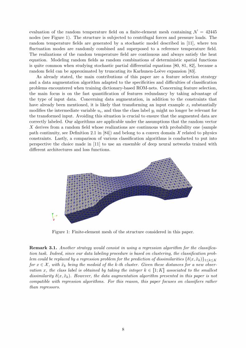
evaluation of the random temperature field on a finite-element mesh containing N = 42445nodes (see Figure 1). The structure is subjected to centrifugal forces and pressure loads. Therandom temperature fields are generated by a stochastic model described in [11], where tenfluctuation modes are randomly combined and superposed to a reference temperature field.The realizations of the random temperature field are continuous and always satisfy the heatequation. Modeling random fields as random combinations of deterministic spatial functionsis quite common when studying stochastic partial differential equations [80, 81, 82], because arandom field can be approximated by truncating its Karhunen-Loeve expansion [83].

As already stated, the main contributions of this paper are a feature selection strategyand a data augmentation algorithm adapted to the specificities and difficulties of classificationproblems encountered when training dictionary-based ROM-nets. Concerning feature selection,the main focus is on the fast quantification of features redundancy by taking advantage ofthe type of input data. Concerning data augmentation, in addition to the constraints thathave already been mentioned, it is likely that transforming an input example xi substantiallymodifies the intermediate variable ui, and thus the class label yi might no longer be relevant forthe transformed input. Avoiding this situation is crucial to ensure that the augmented data arecorrectly labeled. Our algorithms are applicable under the assumptions that the random vectorX derives from a random field whose realizations are continuous with probability one (samplepath continuity, see Definition 2.1 in [84]) and belong to a convex domain X related to physicsconstraints. Lastly, a comparison of various classification algorithms is conducted to put intoperspective the choice made in [11] to use an ensemble of deep neural networks trained withdifferent architectures and loss functions.

Figure 1: Finite-element mesh of the structure considered in this paper.

Remark 3.1. Another strategy would consist in using a regression algorithm for the classifica-tion task. Indeed, since our data labeling procedure is based on clustering, the classification prob-lem could be replaced by a regression problem for the prediction of dissimilarities {δ(x, xk)}1≤k≤Kfor x ∈ X , with xk being the medoid of the k-th cluster. Given these distances for a new obser-vation x, the class label is obtained by taking the integer k ∈ [[1;K]] associated to the smallestdissimilarity δ(x, xk). However, the data augmentation algorithm presented in this paper is notcompatible with regression algorithms. For this reason, this paper focuses on classifiers ratherthan regressors.

8

4 Feature selection

4.1 Feature selection based on mutual information

We recall that a projection π is a linear map satisfying π ◦ π = π. It is entirely defined by itskernel and its image, which are complementary: given two complementary vector subspaces V1and V2, there is a unique projection π whose kernel is V1 and whose image is V2, namely theprojection onto V2 along V1. For more details about projections, see [85], pages 385 to 388. Letus now give a formal definition of a feature selector :

Definition 4.1. (Feature selector) Let V be a finite-dimensional real vector space. Given a basisB = (ei)1≤i≤dim(V ) of V and a set of integers S ⊂ [[1; dim(V )]], the feature selector πS,B : V → Vis the projection whose image is span ({ei}i∈S) and whose kernel is span

({ei}i∈[[1;dim(V )]]\S

).

When the choice of the basis B is obvious, the notation πS,B is simply replaced by πS . Inpractice:

∀(λi)1≤i≤dim(V ) ∈ Rdim(V ), πS

dim(V )∑i=1

λiei

=∑i∈S

λiei (8)

Therefore, from a numerical point of view, one can interpret the feature selector as linear mapπS : V → span ({ei}i∈S), which enables reducing the size of the vector representing πS(x) forx ∈ V . In this way, applying a feature selector πS to a vector of RN consists in masking itsfeatures whose indexes are not in S, which gives a reduced vector in R|S| where |S| denotesthe number of elements in S. Feature selection algorithms build the set S by searching for themost relevant features for the prediction of the output variable Y . For this purpose, the mutualinformation can be used to quantify the degree of the relationship between variables:

Definition 4.2. (Mutual information [86], eq. 8.47, p. 251) Let Z1 and Z2 be two real-valuedrandom variables with joint probability distribution p1,2 and marginal distributions p1 and p2.The mutual information I(Z1, Z2) is defined by:

I(Z1, Z2

)=

∫R2

p1,2(z1, z2) log

(p1,2(z

1, z2)

p1(z1)p2(z2)

)dz1dz2 (9)

The mutual information measures the mutual dependence between two random variables.Contrary to correlation coefficients, the information provided by this score function is not limitedto linear dependence. The mutual information is nonnegative, and equals to zero if and only ifthe random variables are independent. Given Equation (2), replacing Z1 by a feature Xi of Xand Z2 by Y gives:

I(Xi, Y

)=

K∑k=1

PY (k)

∫xi∈R

pXi|Y (xi|k) log

(pXi|Y (xi|k)

pXi(xi)

)dxi (10)

The mutual information can be used to quantify the redundancy of a set of features S and itsrelevance for predicting Y :

Definition 4.3. (Relevance [22], eq. 4, p. 2) Let X = (Xi)1≤i≤N be a multivariate randomvariable, and let Y be a discrete random variable. The relevance of a reduced set S ⊂ [[1;N ]] offeatures of X for predicting Y is defined by:

D(S, Y ) =1

S

∑i∈S

I(Xi, Y ) (11)

9

Definition 4.4. (Redundancy [22], eq. 5, p. 2) Let X = (Xi)1≤i≤N be a multivariate randomvariable. The redundancy of a reduced set S ⊂ [[1;N ]] of features of X is defined by;

R(S) =1

S2

∑i,j∈S2

I(Xi, Xj) (12)

The minimum redundancy maximum relevance (mRMR) algorithm [21, 22] builds the set Sby maximizing D(S, Y ) − R(S), which is a combinatorial optimization problem. For this typeof optimization problem, a brute-force search is intractable, because the number of solutioncandidates is too large. Instead, mRMR searches for a sub-optimal solution by following a greedyapproach. First, the feature having the highest mutual information with the label variable Y isselected. Then, the algorithm follows an incremental procedure: given the set Sm−1 obtained atiteration m− 1, form the set Sm such that:

Sm = Sm−1 ∪

arg maxi∈[[1;N ]]\Sm−1

I(Xi, Y )− 1

m− 1

∑j∈Sm−1

I(Xi, Xj)

(13)

This incremental procedure stops when m reaches the target number of features Nf . A reviewof feature selection algorithms based on mutual information can be found in [87].

4.2 A geostatistical variant of mRMR feature selection

When training dictionary-based ROM-nets, the number of features of the random vector Xscales with the number of nodes N in the mesh. In particular, the number of features is exactlyN if X is the nodal representation of a scalar field. Hence, there are too many features tocompute all redundancy terms I(Xi, Xj). However, one can estimate the redundancy termsthanks to the proximities of the features on the mesh. Indeed, X is a regionalized variable: inour example, we recall that ξi ∈ R3 denotes the position of the i-th node in the mesh, and thatthe feature Xi corresponds to the value taken by a random temperature field at ξi. If two pointsξi and ξj of the mesh are close to each other, the corresponding features Xi and Xj are likelyto be correlated and thus redundant because of the smoothness of the temperature field. Thisidea is also valid when considering physical variables discretized in time.

In this paper, the random temperature field is modeled by a Gaussian random field [84] asin [11], which is a common and simple approach when modeling uncertainties on a physical field.As a consequence, X is a Gaussian random vector and the mutual information I(Xi, Xj) has asimple formula involving the correlation coefficient:

Property 4.5. (Mutual information of two correlated Gaussian random variables [86], eq. 8.56,p. 252) Let (X1, X2) be a Gaussian random vector. The mutual information I(X1, X2) reads:

I(X1, X2) = −1

2ln(1− ρ2

)(14)

where ρ denotes the correlation between X1 and X2.

This property implies that, for Gaussian random fields having isotropic correlation functions3

ρ, the mutual information I(Xi, Xj) only depends on the distance ||ξi − ξj ||2. A wide varietyof isotropic correlation functions are given in [84]. More generally, since Equation (14) is anincreasing function of ρ2, any isotropic upper (resp. lower) bound of the squared correlationfunction gives an isotropic upper (resp. lower) bound of the mutual information.

For the example studied in this paper, Figure 2 shows that the mutual information I(Xi, Xj)decreases as the corresponding distance ||ξi − ξj ||2 increases. Therefore, our feature selection

3The correlation function ρ(ξ, ξ′) of a random field is isotropic if it only depends on the distance ||ξ − ξ′||2.

10

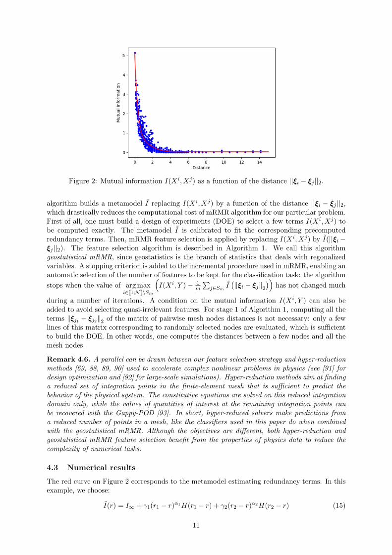
Figure 2: Mutual information I(Xi, Xj) as a function of the distance ||ξi − ξj ||2.

algorithm builds a metamodel I replacing I(Xi, Xj) by a function of the distance ||ξi − ξj ||2,which drastically reduces the computational cost of mRMR algorithm for our particular problem.First of all, one must build a design of experiments (DOE) to select a few terms I(Xi, Xj) tobe computed exactly. The metamodel I is calibrated to fit the corresponding precomputedredundancy terms. Then, mRMR feature selection is applied by replacing I(Xi, Xj) by I(||ξi−ξj ||2). The feature selection algorithm is described in Algorithm 1. We call this algorithmgeostatistical mRMR, since geostatistics is the branch of statistics that deals with regonalizedvariables. A stopping criterion is added to the incremental procedure used in mRMR, enabling anautomatic selection of the number of features to be kept for the classification task: the algorithm

stops when the value of arg maxi∈[[1;N ]]\Sm

(I(Xi, Y )− 1

m

∑j∈Sm

I(‖ξi − ξj‖2

))has not changed much

during a number of iterations. A condition on the mutual information I(Xi, Y ) can also beadded to avoid selecting quasi-irrelevant features. For stage 1 of Algorithm 1, computing all theterms ‖ξj1 − ξj2‖2 of the matrix of pairwise mesh nodes distances is not necessary: only a fewlines of this matrix corresponding to randomly selected nodes are evaluated, which is sufficientto build the DOE. In other words, one computes the distances between a few nodes and all themesh nodes.

Remark 4.6. A parallel can be drawn between our feature selection strategy and hyper-reductionmethods [69, 88, 89, 90] used to accelerate complex nonlinear problems in physics (see [91] fordesign optimization and [92] for large-scale simulations). Hyper-reduction methods aim at findinga reduced set of integration points in the finite-element mesh that is sufficient to predict thebehavior of the physical system. The constitutive equations are solved on this reduced integrationdomain only, while the values of quantities of interest at the remaining integration points canbe recovered with the Gappy-POD [93]. In short, hyper-reduced solvers make predictions froma reduced number of points in a mesh, like the classifiers used in this paper do when combinedwith the geostatistical mRMR. Although the objectives are different, both hyper-reduction andgeostatistical mRMR feature selection benefit from the properties of physics data to reduce thecomplexity of numerical tasks.

4.3 Numerical results

The red curve on Figure 2 corresponds to the metamodel estimating redundancy terms. In thisexample, we choose:

I(r) = I∞ + γ1(r1 − r)α1H(r1 − r) + γ2(r2 − r)α2H(r2 − r) (15)

11

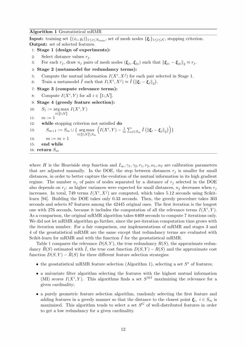
Algorithm 1 Geostatistical mRMR

Input: training set {(xi, yi)}1≤i≤Ntrain , set of mesh nodes {ξi}1≤i≤N , stopping criterion.Output: set of selected features.

1: Stage 1 (design of experiments):

2: Select distance values rj .3: For each rj , draw nj pairs of mesh nodes (ξj1 , ξj2) such that ‖ξj1 − ξj2‖2 ≈ rj .4: Stage 2 (metamodel for redundancy terms):

5: Compute the mutual information I(Xi, Xj) for each pair selected in Stage 1.6: Train a metamodel I such that I(Xi, Xj) ≈ I

(‖ξi − ξj‖2

).

7: Stage 3 (compute relevance terms):

8: Compute I(Xi, Y ) for all i ∈ [[1;N ]].

9: Stage 4 (greedy feature selection):

10: S1 := arg maxi∈[[1;N ]]

I(Xi, Y )

11: m := 112: while stopping criterion not satisfied do

13: Sm+1 := Sm ∪ { arg maxi∈[[1;N ]]\Sm

(I(Xi, Y )− 1

m

∑j∈Sm

I(‖ξi − ξj‖2

))}

14: m := m+ 115: end while16: return Sm

where H is the Heaviside step function and I∞, γ1, γ2, r1, r2, α1, α2 are calibration parametersthat are adjusted manually. In the DOE, the step between distances rj is smaller for smalldistances, in order to better capture the evolution of the mutual information in its high gradientregime. The number nj of pairs of nodes separated by a distance of rj selected in the DOEalso depends on rj : as higher variances were expected for small distances, nj decreases when rjincreases. In total, 749 terms I(Xi, Xj) are computed, which takes 5.12 seconds using Scikit-learn [94]. Building the DOE takes only 0.33 seconds. Then, the greedy procedure takes 303seconds and selects 87 features among the 42445 original ones. The first iteration is the longestone with 276 seconds, because it includes the computation of all the relevance terms I(Xi, Y ).As a comparison, the original mRMR algorithm takes 6469 seconds to compute 7 iterations only.We did not let mRMR algorithm go further, since the per-iteration computation time grows withthe iteration number. For a fair comparison, our implementations of mRMR and stages 3 and4 of the geostatistical mRMR are the same except that redundancy terms are evaluated withScikit-learn for mRMR and with the function I for the geostatistical mRMR.

Table 1 compares the relevance D(S, Y ), the true redundancy R(S), the approximate redun-dancy R(S) estimated with I, the true cost function D(S, Y )−R(S) and the approximate costfunction D(S, Y )− R(S) for three different feature selection strategies:

• the geostatistical mRMR feature selection (Algorithm 1), selecting a set S∗ of features;

• a univariate filter algorithm selecting the features with the highest mutual information(MI) scores I(Xi, Y ). This algorithms finds a set SMI maximizing the relevance for agiven cardinality;

• a purely geometric feature selection algorithm, randomly selecting the first feature andadding features in a greedy manner so that the distance to the closest point ξi, i ∈ Sm ismaximized. This algorithm tends to select a set SG of well-distributed features in orderto get a low redundancy for a given cardinality.

12

Since the geostatistical mRMR automatically selected 87 features, the two other approaches areapplied with |SG| = |SMI | = 87 as a target. Table 1 shows that the relevance of the set S∗

selected by our algorithm is in the same order of magnitude as the relevance of the set SMI . Itsredundancy is in the same order of magnitude as the redundancy of the set SG. These resultsshow that the geostatistical mRMR algorithm does have the desired behavior: it selects a subsetof features S∗ with high relevance and low redundancy. Figure 3 shows the features selectedby the three different algorithms. The classification accuracies of several classifiers using thereduced features S∗ are given in the last section of the article.

Table 1: Evaluation of the geostatistical mRMR feature selection algorithm.

Algorithm D(S, Y ) R(S) R(S) D(S, Y )− R(S) D(S, Y )−R(S)

Geostatistical mRMR (S∗) 0.0460 0.0816 0.1111 −0.0356 −0.0651MI-based filter (SMI) 0.0671 0.9794 0.8129 −0.9124 −0.7458Geometric filter (SG) 0.0090 0.0788 0.1072 −0.0699 −0.0982

Figure 3: Red dots indicate the selected features. From the left to the right: geometric featureselection, MI-based feature selection, geostatistical mRMR.

Remark 4.7. The geometric feature selection algorithm gives rather good results in terms of thecost function, but it does not mean that it is an appropriate approach. Indeed, one can see thatthe relevance of SG is very low, since this algorithm does not use any information concerningthe classification problem.

5 Data augmentation

5.1 Pure sets

Definition 5.1. (Convex set [95], p. 10) Let V be a real vector space. A non-empty set S ⊂ Vis convex if:

∀(x1, x2) ∈ S2, ∀λ ∈ [0; 1], λx1 + (1− λ)x2 ∈ S (16)

Definition 5.2. (Convex combination [95], p. 11) Let {xi}1≤i≤n be a finite set of elements ofa real vector space V . A convex combination of {xi}1≤i≤n is a vector x ∈ V such that:

∃ (λi)1≤i≤n ∈ Rn+ |n∑i=1

λi = 1 and x =n∑i=1

λixi (17)

Definition 5.3. (Convex hull of a set [95], p. 12) Let V be a real vector space and S a non-empty set included in V . The convex hull or convex envelope E(S) of S is the smallest convexset containing S. Equivalently, the convex hull E(S) can be defined as the set of all convexcombinations of all finite subsets of S.

Property 5.4. (Image of a convex hull by a linear map) Let V and W be two real vector spaces,and let L : V →W be a linear map. Let S be a non-empty set included in V . Then:

L (E(S)) = E (L(S)) (18)

13

Proof. Let z ∈ E (L(S)). Following the definition of a convex hull, there exists n ∈ N∗ such that:

∃ (wi)1≤i≤n ∈ L(S)n, ∃ (λi)1≤i≤n ∈ Rn+ |n∑i=1

λi = 1 and z =

n∑i=1

λiwi (19)

For all i ∈ [[1;n]], as wi ∈ L(S), there exists vi ∈ S such that wi = L(vi). By linearity of L:

z =

n∑i=1

λiL(vi) = L

(n∑i=1

λivi

)∈ L (E(S)) (20)

so E (L(S)) ⊂ L (E(S)). The other inclusion can be shown using exactly the same arguments.Thus: L (E(S)) = E (L(S)).

This property has a very simple yet important consequence for the data augmentation algorithmpresented in this paper:

Property 5.5. Let V and W be two real vector spaces, and let L : V → W be a linear map.Let S be a non-empty set included in V . Then, for all x ∈ V :

L(x) /∈ E (L(S))⇒ x /∈ E(S) (21)

Proof. By contraposition, x ∈ E(S)⇒ L(x) ∈ L (E(S)) = E (L(S)).

Our data augmentation strategy uses this property in the particular case where the linear mapis a projection. As a reminder, the notation K stands for the true classifier assigning any inputx to a single label y ∈ [[1;K]]. Before giving the description of the algorithm, let us introducethe definition of pure sets in a labeled dataset and a characterization theorem:

Definition 5.6. (Pure set) Let n be a positive integer, and let S = {xi}1≤i≤n be a finite set ofelements of a real vector space V labeled by K. Let SI = {xi}i∈I⊂[[1;n]] be a non-empty subset ofS. The set SI is pure in S if K (S ∩ E(SI)) is a singleton, which means that the set SI is purein S if all of the points of S that belong to the convex hull of SI have the same label.

Let S = {xi}1≤i≤n be a finite set of elements of a finite-dimensional real vector space Vlabeled by integers {yi}1≤i≤n in [[1;K]], with K ≤ n. For all k ∈ [[1;K]], Ck denotes the set ofelements of S labeled by k:

Ck = {xi ∈ S | yi = k} (22)

For any subset Sk of Ck with cardinality |Sk|, ASk∈ Rdim(V )×|Sk| denotes the matrix whose

columns contain the coordinates of the elements of Sk. The matrix denoted by ASkis obtained

by adding a row of ones below the matrix ASk, giving a matrix of size (1 + dim(V ))× |Sk|.

Theorem 5.7. (Pure set characterization) Let Sk be a subset of Ck with cardinality |Sk|. Theset Sk is pure in S if and only if for all x in S \ Ck the linear system:

ASkw =

(x1

)(23)

has no nonnegative solution w ∈ R|Sk|+ .

Proof. Let x ∈ S \ Ck. Equation (23) has no nonnegative solution if and only if:

@ w ∈ R|Sk|+ |

|Sk|∑i=1

wi = 1 and ASkw = x (24)

⇐⇒ x /∈ E (Sk) (25)

which ends the proof.

14

Corollary 5.8. (Pure set testing) Let Sk be a subset of Ck with cardinality |Sk|, and let L :V →W be a linear map, where W is a finite-dimensional real vector space. If for all x in S \Ckthe linear system:

AL(Sk)w =

(L(x)

1

)(26)

has no nonnegative solution in R|Sk|+ , then Sk is pure in S.

Proof. Equation (26) characterizes the purity of L(Sk) in L(S) (Theorem 5.7), which impliesthat Sk is pure in S (Property 5.5).

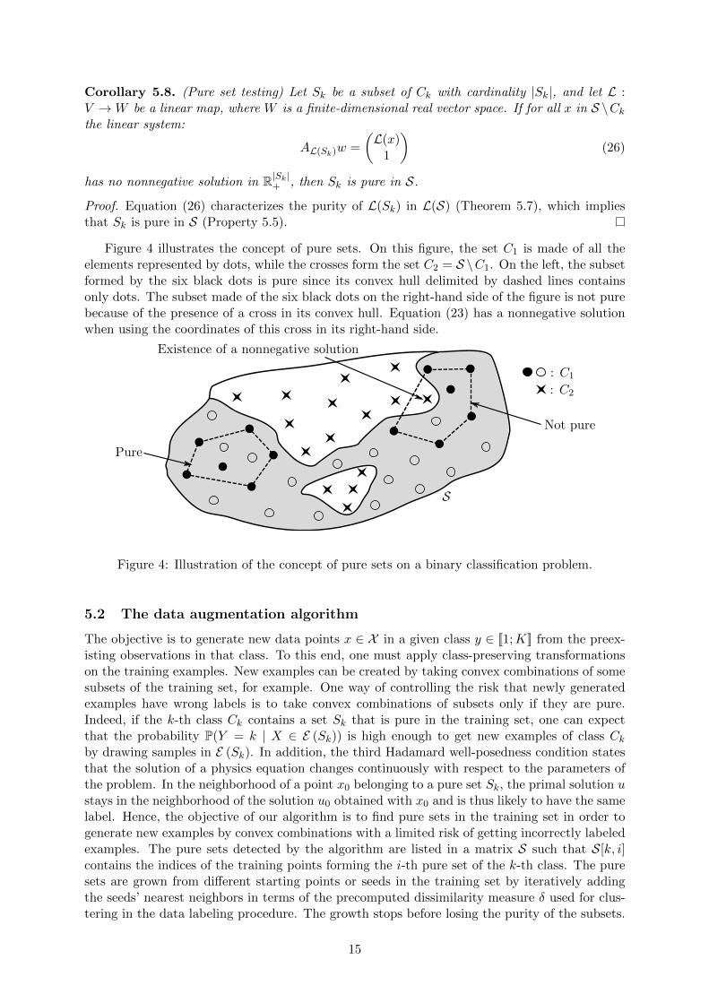
Figure 4 illustrates the concept of pure sets. On this figure, the set C1 is made of all theelements represented by dots, while the crosses form the set C2 = S \C1. On the left, the subsetformed by the six black dots is pure since its convex hull delimited by dashed lines containsonly dots. The subset made of the six black dots on the right-hand side of the figure is not purebecause of the presence of a cross in its convex hull. Equation (23) has a nonnegative solutionwhen using the coordinates of this cross in its right-hand side.

Existence of a nonnegative solution

Not pure

Pure

S

: C1

: C2

Figure 4: Illustration of the concept of pure sets on a binary classification problem.

5.2 The data augmentation algorithm

The objective is to generate new data points x ∈ X in a given class y ∈ [[1;K]] from the preex-isting observations in that class. To this end, one must apply class-preserving transformationson the training examples. New examples can be created by taking convex combinations of somesubsets of the training set, for example. One way of controlling the risk that newly generatedexamples have wrong labels is to take convex combinations of subsets only if they are pure.Indeed, if the k-th class Ck contains a set Sk that is pure in the training set, one can expectthat the probability P(Y = k | X ∈ E (Sk)) is high enough to get new examples of class Ckby drawing samples in E (Sk). In addition, the third Hadamard well-posedness condition statesthat the solution of a physics equation changes continuously with respect to the parameters ofthe problem. In the neighborhood of a point x0 belonging to a pure set Sk, the primal solution ustays in the neighborhood of the solution u0 obtained with x0 and is thus likely to have the samelabel. Hence, the objective of our algorithm is to find pure sets in the training set in order togenerate new examples by convex combinations with a limited risk of getting incorrectly labeledexamples. The pure sets detected by the algorithm are listed in a matrix S such that S[k, i]contains the indices of the training points forming the i-th pure set of the k-th class. The puresets are grown from different starting points or seeds in the training set by iteratively addingthe seeds’ nearest neighbors in terms of the precomputed dissimilarity measure δ used for clus-tering in the data labeling procedure. The growth stops before losing the purity of the subsets.

15

However, checking the purity in the high-dimensional input space can cause difficulties, evenwhen training the data augmentation algorithm after a first dimensionality reduction like in thispaper. For this reason, the algorithm checks the purity after having applied a feature selectorπS with a small random subset of features S containing d features. Let us apply Property 5.5with V = W being the input vector space containing X and with the linear map L being thefeature selector πS . As Property 5.5 states, if no point of πS ({xm}1≤m≤Ntrain \ Ck) belongs tothe convex hull of πS

({xm}m∈S[k,i]

), then the set E

({xm}m∈S[k,i]

)does not contain any point

labeled with k′ 6= k. Since a set can lose its purity after projection, the algorithms tries pmax

random feature selectors πS before considering that the set is not pure. In practice, the purityof πS

({xm}m∈S[k,i]

)in πS ({xm}1≤m≤Ntrain) is numerically tested by solving a nonnegative least

squares (NNLS [96]) problem. If for all points x ∈ {xm}1≤m≤Ntrain \ Ck the inequality:

minw∈R|S[k,i]|+

||AπS({xm}m∈S[k,i])w − πS(x)||2 ≥ εDA||πS(x)||2 (27)

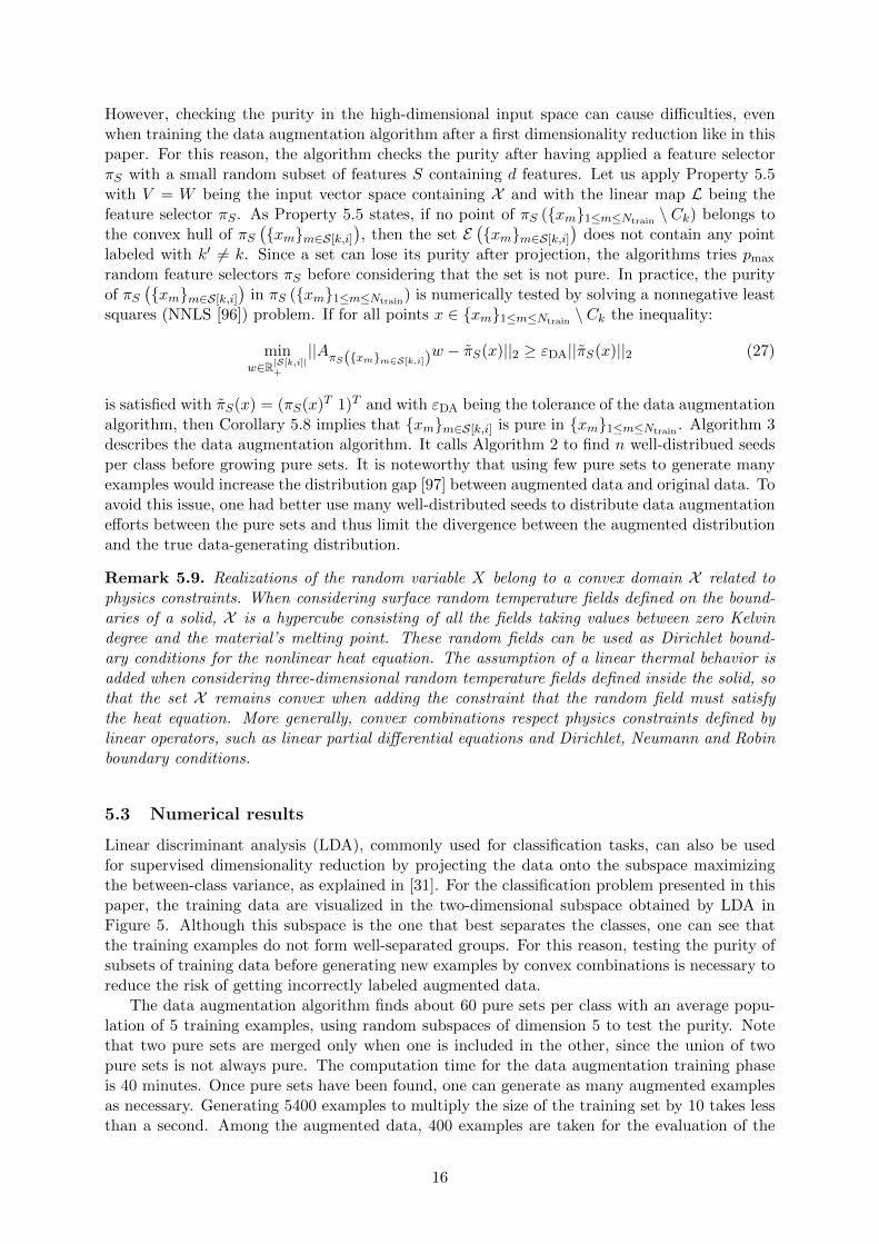
is satisfied with πS(x) = (πS(x)T 1)T and with εDA being the tolerance of the data augmentationalgorithm, then Corollary 5.8 implies that {xm}m∈S[k,i] is pure in {xm}1≤m≤Ntrain . Algorithm 3describes the data augmentation algorithm. It calls Algorithm 2 to find n well-distribued seedsper class before growing pure sets. It is noteworthy that using few pure sets to generate manyexamples would increase the distribution gap [97] between augmented data and original data. Toavoid this issue, one had better use many well-distributed seeds to distribute data augmentationefforts between the pure sets and thus limit the divergence between the augmented distributionand the true data-generating distribution.

Remark 5.9. Realizations of the random variable X belong to a convex domain X related tophysics constraints. When considering surface random temperature fields defined on the bound-aries of a solid, X is a hypercube consisting of all the fields taking values between zero Kelvindegree and the material’s melting point. These random fields can be used as Dirichlet bound-ary conditions for the nonlinear heat equation. The assumption of a linear thermal behavior isadded when considering three-dimensional random temperature fields defined inside the solid, sothat the set X remains convex when adding the constraint that the random field must satisfythe heat equation. More generally, convex combinations respect physics constraints defined bylinear operators, such as linear partial differential equations and Dirichlet, Neumann and Robinboundary conditions.

5.3 Numerical results

Linear discriminant analysis (LDA), commonly used for classification tasks, can also be usedfor supervised dimensionality reduction by projecting the data onto the subspace maximizingthe between-class variance, as explained in [31]. For the classification problem presented in thispaper, the training data are visualized in the two-dimensional subspace obtained by LDA inFigure 5. Although this subspace is the one that best separates the classes, one can see thatthe training examples do not form well-separated groups. For this reason, testing the purity ofsubsets of training data before generating new examples by convex combinations is necessary toreduce the risk of getting incorrectly labeled augmented data.

The data augmentation algorithm finds about 60 pure sets per class with an average popu-lation of 5 training examples, using random subspaces of dimension 5 to test the purity. Notethat two pure sets are merged only when one is included in the other, since the union of twopure sets is not always pure. The computation time for the data augmentation training phaseis 40 minutes. Once pure sets have been found, one can generate as many augmented examplesas necessary. Generating 5400 examples to multiply the size of the training set by 10 takes lessthan a second. Among the augmented data, 400 examples are taken for the evaluation of the

16

Algorithm 2 Seeds selection for data augmentation. Note: all the dissimilarities have alreadybeen computed in the data labeling procedure.

Input: training set {(xi, yi)}1≤i≤Ntrain , class label k, class center xk, dissimilarity matrix δ,target number of seeds n, preselection parameters (ε1, ε2) ∈ [0; 1]2.

Output: List lk of n indices of seeds candidates for the k-th class.1: Stage 1 (filter the data):2: Find the minimum dissimilarity δkref separating the class center xk from a point belonging

to another class.3: Remove points having neighbors belonging to foreign classes within a distance of ε1δ

kref.

4: Remove isolated points having no neighbor within a distance of ε2δkref.

5: Ik := set of the indices of the remaining points in class k.6: Stage 2 (maximin greedy selection):7: Initialize lk with the index of the class center xk.8: for i ∈ [[2; min(n, |Ik| − 1)]] do9: j := arg max

l∈Ik\lkminm∈lk

δlm

10: Append j to lk.11: end for12: return lk

Figure 5: Data visualization in the 2D subspace maximizing the separation between classes(supervised linear dimensionality reduction using LDA).

data augmentation algorithm. The data labeling procedure involving numerical simulations isapplied for these 400 examples in order to estimate the percentage of incorrectly labeled data.It turns out that none of these examples is incorrectly labeled, which validates the algorithmfor our problem. The benefits of data augmentation for the classification task are evaluated inthe final section.

6 Validation of our feature selection and data augmentation al-gorithms

6.1 Classification performances of various classifiers

In this section, 14 different classifiers are trained and evaluated on our classification problem.To evaluate whether the features selected by geostatistical mRMR are relevant for classification

17

Algorithm 3 Data augmentation algorithm

Input: training set {(xi, yi)}1≤i≤Ntrain , dissimilarity matrix δ, per-class number of seeds n,maximum number of pure set testings pmax, dimension d of subspaces for pure set testings,number of augmented data NDA.

Output: augmented data {(xi, yi)}1≤i≤NDAand matrix S listing pure sets.

1: Stage 1 (find pure sets in the training set):2: for k ∈ [[1;K]] do3: Apply Algorithm 2 to get the list lk of n indices of seeds candidates.4: for i ∈ [[1;n]] do5: S1 := {lk[i]}6: neighbors := argsort(δ[lk[i], :])7: j := 18: setPurity := True9: while setPurity do

10: Sj+1 := Sj ∪ {neighbors[j]}11: j := j + 112: p := 113: Select a random subset S of d features.14: while {πS(xm)}m∈Sj is not pure in {πS(xm)}1≤m≤Ntrain and p ≤ pmax do15: Select a new random subset S of d features.16: p := p+117: end while18: if p = pmax + 1 then19: setPurity := False20: end if21: end while22: S[k, i] := Sj−123: end for24: end for25: Stage 2 (generate new data):26: GenerateNDA random convex combinations {xi}1≤i≤NDA

of the pure sets listed in S. Convexcombinations xi of the pure set described in S[k, j] are labeled by yi = k.

27: return {(xi, yi)}1≤i≤NDAand S

18

purposes, each classifier is tested twice: once in combination with the geostatistical mRMR andonce with principal component analysis (PCA) with 10 modes. Since the random temperaturefields derive from a Gaussian random field involving only 10 modes, the database obtainedafter applying PCA contains all the information of the original data. Each combination of oneof the 14 classifiers with PCA or feature selection is trained twice: once on the true trainingset containing Ntrain = 600 examples, and once on the augmented training set made of 6000examples.

All the classifiers are trained with Scikit-learn [94], except multilayer perceptrons (MLPs)and radial basis function networks (RBFNs) which are trained with PyTorch [98]. We train theRBFNs in a fully supervised manner, which means that the parameters of the radial basis func-tions are learnt by gradient descent like the weights of the fully-connected layers. In addition,we use only one hidden layer for RBFNs, since these artificial neural networks generally haveshallow architectures, as explained in [99]. Deeper architectures have been tested for MLPs.Scikit-learn’s MLP classifier has also been tested; it is called simple MLP in this paper, becauseits architecture is only made of fully-connected layers and does not include dropout [100] norbatch normalization [101]. All the classifiers based on artificial neural networks are trained withTikhonov regularization and early stopping [19]. Logistic regression is trained with elastic netregularization [102]. Kernels used for support vector machines (SVMs) are obtained by combin-ing several polynomial kernels with different hyperparameters. Kernel design could be optimizedusing multiple kernel learning algorithms [103], but we simply build our kernels by evaluatingdifferent combinations on the validation set, just as when we look for a good architecture forartificial neural networks.

The classification accuracies on test data are given in Table 2. Of course, this rankingis specific to the classification problem presented in this paper, no general conclusion can bedrawn from this particular numerical application. On this classification problem, when usingaugmented data in the training phase, the highest test accuracy reached with linear classifiersis 43.5%, obtained with the linear SVM combined with PCA. The fact that k-nearest neighborsclassifiers barely exceed 50.0% of accuracy on this problem is related to an observation that wasmade in [11]: there is no simple correlation between the Euclidean distance and the physics-informed dissimilarity measure used in dictionary-based ROM-nets. MLPs get the best results,reaching 87.0% of accuracy when combined with our data augmentation and feature selectionalgorithms. Interestingly, quadratic discriminant analysis (QDA) gives excellent results whilehaving no hyperparameter to tune, contrary to the two other families of classifiers obtaining thebest results, namely MLPs and multiple kernel SVMs. This makes QDA the best compromisebetween accuracy and training complexity for this specific classification task.

Although PCA perfectly describes the input data in this example, the geostatistical mRMRfeature selection algorithm enables reaching higher accuracies with some classifiers. Not only itbehaves as the original mRMR when selecting features, but it also gives satisfying results whencombined with a classifier. Concerning data augmentation, Table 2 shows that our algorithmsignificantly improves classification results. The accuracy gain due to data augmentation is4.98% on average and ranges from −2.5% to 10.5%, increasing the accuracy in 25 cases out of28.

6.2 How to further improve classification performances?

Ensemble methods can be used to reduce overfitting and increase the accuracy on test data.In addition, it enables recycling different variants of a classifier that the user has trained fordifferent hyperparameters. Using ensemble averaging with classifiers trained on the augmenteddataset with feature selection, we manage to combine 6 MLPs with different architectures toreach an accuracy of 89.0%. When stacking these MLPs with a ridge logistic regression analyzingthe predicted membership probabilities, we get an accuracy of 90.0%. In addition to ensemblelearning methods, one can also use random noise injection to increase noise robustness, as

19

Table 2: Test accuracies of different classifiers with dimensionality reduction viaprincipal component analysis (PCA) or feature selection (FS), with and withoutdata augmentation (DA).

Classifier Dim. red. Acc. with DA Acc. without DA

Stacking (6 MLPs and logistic regression) FS 90.0% −Ensemble averaging (6 MLPs) FS 89.0% −

Multilayer perceptron FS 87.0% 81.0%Multilayer perceptron PCA 86.5% 81.5%

Simple multilayer perceptron PCA 85.0% 79.5%Simple multilayer perceptron FS 84.0% 80.0%

Quadratic discriminant analysis FS 77.5% 70.5%Quadratic discriminant analysis PCA 76.0% 70.0%

Multiple kernel support vector machine PCA 73.0% 68.0%Multiple kernel support vector machine FS 72.5% 66.0%

Random forest FS 69.0% 63.0%AdaBoost FS 68.5% 63.0%

Gradient-boosted trees FS 68.0% 58.5%Radial basis function network PCA 63.5% 62.0%Radial basis function network FS 62.5% 60.0%

Decision tree FS 55.5% 43.5%k-nearest neighbors PCA 51.0% 46.0%

AdaBoost PCA 50.5% 52.5%k-nearest neighbors FS 50.0% 47.0%

Gradient-boosted trees PCA 49.5% 48.0%Random forest PCA 45.0% 47.5%

Linear support vector machine PCA 43.5% 33.0%Linear support vector machine FS 40.5% 34.5%

Gaussian naive Bayes FS 39.5% 34.5%Gaussian naive Bayes PCA 38.5% 31.5%

Penalized logistic regression PCA 38.5% 28.0%Penalized logistic regression FS 37.0% 29.0%

Decision tree PCA 34.0% 36.5%Linear discriminant analysis PCA 33.5% 29.0%Linear discriminant analysis FS 32.5% 29.0%

explained in [19].

7 Conclusion

Classification algorithms are used in computational physics for automatic model recommenda-tion. Such modeling strategies enable the reduction of the computation time, or the selectionbetween models with different physics when one wants to improve the accuracy of numericalpredictions. This article deals with the specificities of the classification problems encounteredin computational physics, and more particularly for dictionary-based ROM-nets. These classi-fication problems generally have the three following issues: the lack of training data, their highdimensionality, and the non-applicability of common data augmentation techniques to physicsdata. To tackle these difficulties, two algorithms are proposed. The first one is a geostatisticalvariant of the mRMR feature selection algorithm, enabling the identification of a reduced setof relevant but non-redundant features for high-dimensional regionalized variables. The sec-ond one is a data augmentation algorithm controlling the risk of generating new examples with

20

wrong labels by finding pure subsets in the training set. The performances and benefits of thesealgorithms are illustrated on a classification problem for which 14 classifiers are evaluated.

Acknowledgements

The authors wish to thank Sebastien Da Veiga (SafranTech) for his sound advice, as well as FelipeBordeu (SafranTech) and Julien Cortial (SafranTech) who implemented the Python libraryBasicTools (https://gitlab.com/drti/basic-tools) with FC.

Funding

Study funded by Safran and ANRT (Association Nationale de la Recherche et de la Technologie,France).

References

[1] Y. LeCun, B. Boser, J. S. Denker, D. Henderson, R. E. Howard, W. Hubbard, and L. D.Jackel. Backpropagation applied to handwritten zip code recognition. Neural Computation,1(4):541–551, 1989.

[2] B. Baharudin, L.H. Lee, K. Khan, and A. Khan. A review of machine learning algorithmsfor text-documents classification. Journal of Advances in Information Technology, 1, 022010.

[3] K. Kourou, T.P. Exarchos, K.P. Exarchos, M.V. Karamouzis, and D.I. Fotiadis. Machinelearning applications in cancer prognosis and prediction. Computational and StructuralBiotechnology Journal, 13:8 – 17, 2015.

[4] B. Peherstorfer, D. Butnaru, K. Willcox, and H.J. Bungartz. Localized Discrete EmpiricalInterpolation Method. SIAM Journal on Scientific Computing, 36, 01 2014.

[5] F. Nguyen, S.M. Barhli, D.P. Munoz, and D. Ryckelynck. Computer vision with errorestimation for reduced order modeling of macroscopic mechanical tests. Complexity, 2018.

[6] F. Fritzen, M. Fernandez, and F. Larsson. On-the-fly adaptivity for nonlinear twoscalesimulations using artificial neural networks and reduced order modeling. Frontiers inMaterials, 6:75, 2019.

[7] R. Maulik, O. San, J. Jacob, and C. Crick. Sub-grid scale model classification and blendingthrough deep learning. Journal of Fluid Mechanics, 870:784–812, 07 2019.

[8] M.G. Kapteyn, D.J. Knezevic, and K.E. Willcox. Toward predictive digital twins viacomponent-based reduced-order models and interpretable machine learning.

[9] M.G. Kapteyn and K.E. Willcox. From physics-based models to predictive digital twinsvia interpretable machine learning, 2020.

[10] R. Maulik, O. San, and J.D. Jacob. Spatiotemporally dynamic implicit large eddy simu-lation using machine learning classifiers. Physica D: Nonlinear Phenomena, 406:132409,2020.

[11] T. Daniel, F. Casenave, N. Akkari, and D. Ryckelynck. Model order reduction assisted bydeep neural networks (ROM-net). Adv. Model. and Simul. in Eng. Sci., 7(16), 2020.

21

[12] A. Quarteroni and G. Rozza. Reduced Order Methods for Modeling and ComputationalReduction. Springer Publishing Company, Incorporated, 2013.

[13] W. Keiper, A. Milde, and S. Volkwein. Reduced-Order Modeling (ROM) for Simulation andOptimization: Powerful Algorithms as Key Enablers for Scientific Computing. SpringerInternational Publishing, 2018.

[14] G.D. Smith. Numerical Solution of Partial Differential Equations: Finite Difference Meth-ods. Oxford applied mathematics and computing science series. Clarendon Press, 1985.

[15] A. Ern and J.L. Guermond. Theory and Practice of Finite Elements. Applied Mathemat-ical Sciences. Springer New York, 2013.

[16] H.K. Versteeg and W. Malalasekera. An Introduction to Computational Fluid Dynamics:The Finite Volume Method. Pearson Education Limited, 2007.

[17] W. Borutzky. Bond Graph Modelling of Engineering Systems: Theory, Applications andSoftware Support. SpringerLink : Bucher. Springer New York, 2011.

[18] G. Chandrashekar and F. Sahin. A survey on feature selection methods. Computers andElectrical Engineering, 40(1):16 – 28, 2014.

[19] I. Goodfellow, Y. Bengio, and A. Courville. Deep Learning. MIT Press, 2016. http:

//www.deeplearningbook.org.

[20] A. Janecek, W. Gansterer, M. Demel, and G. Ecker. On the relationship between featureselection and classification accuracy. Journal of Machine Learning Research - ProceedingsTrack, 4:90–105, 01 2008.

[21] C. Ding and H. Peng. Minimum redundancy feature selection from microarray gene ex-pression data. In Computational Systems Bioinformatics. CSB2003. Proceedings of the2003 IEEE Bioinformatics Conference. CSB2003, pages 523–528, Aug 2003.

[22] H. Peng, F. Long, and C. Ding. Feature selection based on mutual information: Criteriaof max-dependency,max-relevance, and min-redundancy. IEEE transactions on patternanalysis and machine intelligence, 27:1226–38, 09 2005.

[23] D. Hua. A regularity result for boundary value problems on Lipschitz domains. Annalesde la Faculte des sciences de Toulouse : Mathematiques, Ser. 5, 10(2):325–333, 1989.

[24] I. Goodfellow, J. Pouget-Abadie, M. Mirza, B. Xu, D. Warde-Farley, S. Ozair, A. Courville,and Y. Bengio. Generative adversarial networks. Advances in Neural Information Pro-cessing Systems, 3, 06 2014.

[25] N. Akkari, F. Casenave, M.E. Perrin, and D. Ryckelynck. Deep Convolutional GenerativeAdversarial Networks Applied to 2D Incompressible and Unsteady Fluid Flows, pages 264–276. 07 2020.

[26] N. Chawla, K. Bowyer, L. Hall, and W. Kegelmeyer. Smote: Synthetic minority over-sampling technique. J. Artif. Intell. Res. (JAIR), 16:321–357, 01 2002.

[27] H. He, Y. Bai, E. Garcia, and S. Li. Adasyn: Adaptive synthetic sampling approach forimbalanced learning. pages 1322 – 1328, 07 2008.

[28] R.E. Bellman. Adaptive control processes. Princeton University Press, 1961.

[29] V.N. Vapnik. Statistical Learning Theory. Wiley-Interscience, 1998.

22

[30] K. Crammer and Y. Singer. On the algorithmic implementation of multiclass kernel-basedvector machines. J. Mach. Learn. Res., 2:265–292, 2002.

[31] T. Hastie, R. Tibshirani, and J.H. Friedman. The Elements of Statistical Learning: DataMining, Inference, and Prediction, 2nd Edition. Springer series in statistics. Springer,2009.

[32] J. Berkson. Application of the logistic function to bio-assay. Journal of the AmericanStatistical Association, 39(227):357–365, 1944.

[33] D.R. Cox. The regression analysis of binary sequences. Journal of the Royal StatisticalSociety. Series B (Methodological), 20(2):215–242, 1958.

[34] D.R. Cox. Some procedures connected with the logistic qualitative response curve. Re-search papers in probability and statistics, pages 55–71, 1966.

[35] C. Cortes and V. Vapnik. Support-vector networks. Mach. Learn., 20(3):273–297, Septem-ber 1995.

[36] B. Boser, I. Guyon, and V. Vapnik. A training algorithm for optimal margin classifier.Proceedings of the Fifth Annual ACM Workshop on Computational Learning Theory, 5,08 1996.

[37] J. Mercer and A.R. Forsyth. Xvi. functions of positive and negative type, and theirconnection the theory of integral equations. Philosophical Transactions of the Royal Societyof London. Series A, Containing Papers of a Mathematical or Physical Character, 209(441-458):415–446, 1909.

[38] A.G. Ivakhnenko and V.G. Lapa. Cybernetic predicting devices. 1966.

[39] R. D. Joseph. Contributions to perceptron theory. phd thesis, cornell univ. 1961.

[40] J. Schmidhuber. Deep learning in neural networks: An overview. Neural networks : theofficial journal of the International Neural Network Society, 61:85–117, 2015.

[41] L. Breiman, J.H. Friedman, R.A. Olshen, and R.A. Stone. Classification and regressiontrees. 1983.

[42] M. E. Maron. Automatic indexing: An experimental inquiry. J. ACM, 8(3):404–417, July1961.

[43] H. Zhang. The optimality of naive bayes. volume 2, 01 2004.

[44] Cover, T. and Hart, P. Nearest neighbor pattern classification. IEEE Transactions onInformation Theory, 13(1):21–27, 1967.

[45] R. Caruana and A. Niculescu-Mizil. An empirical comparison of supervised learning al-gorithms. Proceedings of the 23rd international conference on Machine learning - ICML’06, 2006:161–168, 06 2006.

[46] S. Kotsiantis. Supervised machine learning: A review of classification techniques. Infor-matica (Ljubljana), 31, 10 2007.

[47] M. Perez-Ortiz, S. Jimenez-Fernandez, P.A. Gutierrez, E. Alexandre, C. Martinez, andS. Salcedo-Sanz. A review of classification problems and algorithms in renewable energyapplications. Energies, 9:607, 08 2016.

[48] L. Breiman. Bagging predictors. Machine Learning, 24:123–140, 1996.

23

[49] Tin Kam Ho. The random subspace method for constructing decision forests. IEEE Trans.Pattern Anal. Mach. Intell., 20:832–844, 1998.

[50] D.H. Wolpert. Stacked generalization. Neural Networks, 5:241–259, 1992.

[51] Y. Freund and R.E. Schapire. A decision-theoretic generalization of on-line learning andan application to boosting. In EuroCOLT, 1995.

[52] T.J. Hastie, S. Rosset, J. Zhu, and H. Zou. Multi-class adaboost. 2009.

[53] J. Friedman. Greedy function approximation: A gradient boosting machine. The Annalsof Statistics, 29, 11 2000.

[54] J. Friedman. Stochastic gradient boosting. Computational Statistics and Data Analysis,38:367–378, 02 2002.

[55] L. Mason, J. Baxter, P. Bartlett, and M. Frean. Boosting algorithms as gradient descentin function space. 06 1999.

[56] L. Mason, J. Baxter, P. Bartlett, and M. Frean. Boosting algorithms as gradient descent.pages 512–518, 01 1999.

[57] S. Haykin. Neural Networks - A Comprehensive Foundation. Second edition, pages 351–391, 1999.

[58] L. Breiman. Random forests. Machine Learning, 45:5–32, 2001.

[59] C. Meneveau and P. Sagaut. Large Eddy Simulation for Incompressible Flows: An Intro-duction. Scientific Computation. Springer Berlin Heidelberg, 2006.

[60] F. Feyel. Multiscale FE2 elastoviscoplastic analysis of composite structures. ComputationalMaterials Science, 16(1):344 – 354, 1999.

[61] F. Fritzen and O. Kunc. Two-stage data-driven homogenization for nonlinear solids usinga reduced order model. European Journal of Mechanics - A/Solids, 69:201 – 220, 2018.

[62] D. Bertsimas and J. Dunn. Optimal classification trees. Machine Learning, 106, 04 2017.

[63] Phuong Huynh, D.B., Knezevic, D.J., and Patera, A.T. A static condensation reducedbasis element method : approximation and a posteriori error estimation. ESAIM: M2AN,47(1):213–251, 2013.

[64] J. Eftang, D. Huynnh, D. Knezevic, E. Ronqust, and A. Patera. Adaptive port reductionin static condensation. 01 2015.

[65] J. Eftang and A. Patera. Port reduction in parametrized component static condensation:Approximation and a posteriori error estimation. International Journal for NumericalMethods in Engineering, 96, 07 2013.

[66] K. Smetana and A. Patera. Optimal local approximation spaces for component-basedstatic condensation procedures. SIAM Journal on Scientific Computing, 38:A3318–, 102016.

[67] S. Chaturantabut and D. Sorensen. Discrete empirical interpolation for nonlinear modelreduction. Decision and Control, 2009 held jointly with the 2009 28th Chinese ControlConference, CDC/CCC 2009, Proceedings of the 48th IEEE Conference, pages 4316–4321,2010.

24

[68] J.B. MacQueen. Some methods for classification and analysis of multivariate observations.Proceedings of 5-th Berkeley Symposium on Mathematical Statistics and Probability, 1:281–297, 1967.

[69] D. Ryckelynck. A priori hyperreduction method: an adaptive approach. Journal of Com-putational Physics, Elsevier, 202(1):346–366, 2005.

[70] J. Gu, Z. Wang, J. Kuen, L. Ma, A. Shahroudy, B. Shuai, T. Liu, X. Wang, G. Wang,J. Cai, and T. Chen. Recent advances in convolutional neural networks. Patter Recognition,77:354–377, 2018.

[71] L. Adrian, R.J. Adrian, and J. Westerweel. Particle Image Velocimetry. CambridgeAerospace Series. Cambridge University Press, 2011.

[72] T. Chu, W. Ranson, and M. Sutton. Applications of digital-image-correlation techniquesto experimental mechanics. Experimental Mechanics, 25:232–244, 09 1985.

[73] H. Mueller. Theory of photoelasticity in amorphous solids. Physics, 6(6):179–184, 1935.

[74] U. Fey and Y. Egami. Transition detection by temperature-sensitive paint. volume Chap.7.4 of Handbook with DVD-ROM, pages 537–552. Springer Berlin, Heidelberg, New York,2007.

[75] K. Ye and L.H. Lim. Schubert varieties and distances between subspaces of differentdimensions. SIAM J. Matrix Anal. Appl., 37(3):1176–1197, 2016.

[76] H.S. Park and C.H. Jun. A simple and fast algorithm for k-medoids clustering. ExpertSystems with Applications, 36:3336–3341, 2009.

[77] E. Schubert and P.J. Rousseeuw. Faster k-medoids clustering: Improving the PAM,CLARA, and CLARANS algorithms. In G. Amato, C. Gennaro, V. Oria, andM. Radovanovic, editors, Similarity Search and Applications, pages 171–187, Cham, 2019.Springer International Publishing.

[78] L. Kaufmann and P. Rousseeuw. Clustering by means of medoids. Data Analysis basedon the L1-Norm and Related Methods, pages 405–416, 01 1987.

[79] J.L. Chaboche. A review of some plasticity and viscoplasticity constitutive theories. In-ternational Journal of Plasticity, 24(10):1642 – 1693, 2008. Special Issue in Honor ofJean-Louis Chaboche.

[80] H.G. Matthies, C.E. Brenner, C.G. Bucher, and C. Guedes Soares. Uncertainties in prob-abilistic numerical analysis of structures and solids - Stochastic finite elements. StructuralSafety, 19(3):283 – 336, 1997. Devoted to the work of the Joint Committee on StructuralSafety.

[81] B. Sudret and A. Der Kiureghian. Stochastic finite element methods and reliability: Astate-of-the-art report. 01 2000.

[82] H.G. Matthies and A. Keese. Galerkin methods for linear and nonlinear elliptic stochasticpartial differential equations. Computer Methods in Applied Mechanics and Engineer-ing, 194(12):1295 – 1331, 2005. Special Issue on Computational Methods in StochasticMechanics and Reliability Analysis.

[83] B. N. Khoromskij, A. Litvinenko, and H. G. Matthies. Application of Hierarchical Matricesfor computing the Karhunen-Loeve Expansion. Computing, 84(1–2):49–67, 2009.

25

[84] P. Abrahamsen. A Review of Gaussian Random Fields and Correlation Functions. NorskRegnesentral - Norwegian Computing Center, 1997.

[85] C. Meyer. Matrix Analysis and Applied Linear Algebra Book and Solutions Manual. 012000.

[86] T.M. Cover and J.A. Thomas. Elements of Information Theory. Wiley, 2012.

[87] J. Vergara and P. Estevez. A review of feature selection methods based on mutual infor-mation. Neural Computing and Applications, 24, 01 2014.

[88] M. Barrault, Y. Maday, N.C. Nguyen, and A.T. Patera. An empirical interpolationmethod: application to efficient reduced-basis discretization of partial differential equa-tions. Comptes Rendus Mathematiques, 339(9):666–672, 2004.

[89] C. Farhat, P. Avery, T. Chapman, and J. Cortial. Dimensional reduction of nonlinear

finite element dynamic models with

finite rotations and energy-based mesh sampling and weighting for computational effi-ciency. International Journal for Numerical Methods in Engineering, 98(9):625–662, 2014.

[90] J.A. Hernandez, M.A. Caicedo, and A. Ferrer. Dimensional hyper-reduction of nonlinearfinite element models via empirical cubature. Computer methods in applied mechanics andengineering, 313:687–722, 2017.

[91] D. Amsallem, M. Zahr, Y. Choi, and C. Farhat. Design optimization using hyper-reduced-order models. Structural and Multidisciplinary Optimization, 51:919–940, 04 2014.

[92] F. Casenave, N. Akkari, F. Bordeu, C. Rey, and D. Ryckelynck. A nonintrusive distributedreduced-order modeling framework for nonlinear structural mechanics -Application to elas-toviscoplastic computations. International Journal for Numerical Methods in Engineering,121(1):32–53, 2020.

[93] R. Everson and L. Sirovich. Karhunen-Loeve procedure for gappy data. JOSA A, 12, 081995.

[94] F. Pedregosa, G. Varoquaux, A. Gramfort, V. Michel, B. Thirion, O. Grisel, M. Blon-del, P. Prettenhofer, R. Weiss, V. Dubourg, J. Vanderplas, A. Passos, D. Cournapeau,M. Brucher, M. Perrot, and E. Duchesnay. Scikit-learn: Machine learning in Python.Journal of Machine Learning Research, 12:2825–2830, 2011.

[95] R.T. Rockafellar. Convex Analysis. Princeton Landmarks in Mathematics and Physics.Princeton University Press, 1970.

[96] C.L. Lawson and R.J. Hanson. Solving Least Squares Problems. Society for Industrial andApplied Mathematics, 1995.

[97] Z. He, L. Xie, X. Chen, Y. Zhang, Y. Wang, and Q. Tian. Data augmentation revisited:Rethinking the distribution gap between clean and augmented data. 09 2019.

[98] A. Paszke, S. Gross, F. Massa, A. Lerer, J. Bradbury, G. Chanan, T. Killeen, Z. Lin,N. Gimelshein, L. Antiga, A. Desmaison, A. Kopf, E. Yang, Z. DeVito, M. Raison, A. Te-jani, S. Chilamkurthy, B. Steiner, L. Fang, J. Bai, and S. Chintala. Pytorch: An imperativestyle, high-performance deep learning library. In H. Wallach, H. Larochelle, A. Beygelz-imer, F. d'Alche-Buc, E. Fox, and R. Garnett, editors, Advances in Neural InformationProcessing Systems 32, pages 8026–8037. Curran Associates, Inc., 2019.

26

[99] C.C. Aggarwal. Neural Networks and Deep Learning. Springer, 2018.

[100] N. Srivastava, G. Hinton, A. Krizhevsky, I. Sutskever, and R. Salakhutdinov. Dropout:A simple way to prevent neural networks from overfitting. Journal of Machine LearningResearch, 15:1929–1958, 06 2014.

[101] S. Ioffe and C. Szegedy. Batch normalization: Accelerating deep network training byreducing internal covariate shift. 02 2015.

[102] H. Zou and T. Hastie. Regularization and variable selection via the elastic net. 67(2):301–320, 2005.

[103] M. Gonen and E. Alpaydin. Multiple kernel learning algorithms. Journal of MachineLearning Research, 12:2211–2268, 07 2011.

27