This page intentionally left blank Bumi... · 3.3.1 The BFGS algorithm 29 3.4 Geometry optimization...
245
Transcript of This page intentionally left blank Bumi... · 3.3.1 The BFGS algorithm 29 3.4 Geometry optimization...

This page intentionally left blank

VARIATIONAL PRINCIPLES AND METHODS INTHEORETICAL PHYSICS AND CHEMISTRY
This book brings together the essential ideas and methods behind current applica-tions of variational theory in theoretical physics and chemistry. The emphasis is onunderstanding physical and computational applications of variational methodologyrather than on rigorous mathematical formalism.
The text begins with an historical survey of familiar variational principles inclassical mechanics and optimization theory, then proceeds to develop the vari-ational principles and formalism behind current computational methodology forbound and continuum quantum states of interacting electrons in atoms, molecules,and condensed matter. It covers multiple scattering theory, as applied to electronsin condensed matter and in large molecules. The specific variational principlesdeveloped for electron scattering are then extended to include a detailed presenta-tion of contemporary methodology for electron-impact rotational and vibrationalexcitation of molecules. The book also provides an introduction to the variationaltheory of relativistic fields, including a detailed treatment of Lorentz and gaugeinvariance for the nonabelian gauge field of modern electroweak theory.
Ideal for graduate students and researchers in any field that uses variationalmethodology, this book is particularly suitable as a backup reference for lecturecourses in mathematical methods in physics and theoretical chemistry.
Robert K. Nesbet obtained his BA in physics from Harvard College in 1951and his PhD from the University of Cambridge in 1954. He was then a researchassociate in MIT for two years, before becoming Assistant Professor of Physicsat Boston University. He did research at RIAS, Martin Company, Baltimore, theInstitut Pasteur, Paris and Brookhaven National Laboratory, before becoming aStaff Member at IBM Almaden Research Center in San Jose in 1962. He acted asan Associate Editor for the Journal of Computational Physics and the Journal ofChemical Physics, between 1969 and 1974, and was a visiting professor at severaluniversities throughout the world. Professor Nesbet officially retired in 1994, buthas continued his research and visiting since then. Over the years he has writtenmore than 270 publications in computational physics, atomic and molecular physics,theoretical chemistry, and solid-state physics.


VARIATIONAL PRINCIPLES ANDMETHODS IN THEORETICALPHYSICS AND CHEMISTRY
ROBERT K. NESBETIBM Almaden Research Center

The Pitt Building, Trumpington Street, Cambridge, United Kingdom
The Edinburgh Building, Cambridge CB2 2RU, UK40 West 20th Street, New York, NY 10011-4211, USA477 Williamstown Road, Port Melbourne, VIC 3207, AustraliaRuiz de Alarcón 13, 28014 Madrid, SpainDock House, The Waterfront, Cape Town 8001, South Africa
http://www.cambridge.org
First published in printed format
ISBN 0-521-80391-8 hardbackISBN 0-511-04162-4 eBook
Robert K. Nesbet 2004
2002
(netLibrary)
©

To Anne, Susan, and Barbara


Contents
Preface page xiiiI Classical mathematics and physics 1
1 History of variational theory 31.1 The principle of least time 41.2 The variational calculus 5
1.2.1 Elementary examples 71.3 The principle of least action 8
2 Classical mechanics 112.1 Lagrangian formalism 11
2.1.1 Hamilton’s variational principle 122.1.2 Dissipative forces 122.1.3 Lagrange multiplier method for constraints 13
2.2 Hamiltonian formalism 142.2.1 The Legendre transformation 142.2.2 Transformation from Lagrangian to Hamiltonian 152.2.3 Example: the central force problem 16
2.3 Conservation laws 172.4 Jacobi’s principle 182.5 Special relativity 20
2.5.1 Relativistic mechanics of a particle 212.5.2 Relativistic motion in an electromagnetic field 22
3 Applied mathematics 253.1 Linear systems 253.2 Simplex interpolation 26
3.2.1 Extremum in n dimensions 273.3 Iterative update of the Hessian matrix 28
3.3.1 The BFGS algorithm 293.4 Geometry optimization for molecules 30
vii

viii Contents
3.4.1 The GDIIS algorithm 313.4.2 The BERNY algorithm 31
II Bound states in quantum mechanics 334 Time-independent quantum mechanics 35
4.1 Variational theory of the Schrodinger equation 364.1.1 Sturm–Liouville theory 364.1.2 Idiosyncracies of the Schrodinger equation 384.1.3 Variational principles for the Schrodinger equation 404.1.4 Basis set expansions 41
4.2 Hellmann–Feynman and virial theorems 434.2.1 Generalized Hellmann–Feynman theorem 434.2.2 The hypervirial theorem 434.2.3 The virial theorem 44
4.3 The N -electron problem 454.3.1 The N -electron Hamiltonian 454.3.2 Expansion in a basis of orbital wave functions 464.3.3 The interelectronic Coulomb cusp condition 48
4.4 Symmetry-adapted functions 494.4.1 Algorithm for constructing symmetry-adapted
functions 504.4.2 Example of the method 51
5 Independent-electron models 535.1 N -electron formalism using a reference state 54
5.1.1 Fractional occupation numbers 555.1.2 Janak’s theorem 56
5.2 Orbital functional theory 575.2.1 Explicit components of the energy functional 575.2.2 Orbital Euler–Lagrange equations 585.2.3 Exact correlation energy 59
5.3 Hartree–Fock theory 615.3.1 Closed shells – unrestricted Hartree–Fock (UHF) 615.3.2 Brillouin’s theorem 625.3.3 Open-shell Hartree–Fock theory (RHF) 625.3.4 Algebraic Hartree–Fock: finite basis expansions 645.3.5 Multiconfiguration SCF (MCSCF) 64
5.4 The optimized effective potential (OEP) 655.4.1 Variational formulation of OEP 67
5.5 Density functional theory (DFT) 685.5.1 The Hohenberg–Kohn theorems 685.5.2 Kohn–Sham equations 70

Contents ix
5.5.3 Functional derivatives and local potentials 715.5.4 Thomas–Fermi theory 725.5.5 The Kohn–Sham construction 74
6 Time-dependent theory and linear response 776.1 The time-dependent Schrodinger equation for one electron 786.2 The independent-electron model as a quantum field theory 796.3 Time-dependent Hartree–Fock (TDHF) theory 81
6.3.1 Operator form of Hartree–Fock equations 816.3.2 The screening response 81
6.4 Time-dependent orbital functional theory (TOFT) 836.4.1 Remarks on time-dependent theory 836.4.2 Exact linear response theory 846.4.3 Definition of the response kernel 84
6.5 Reconciliation of N -electron theory and orbital models 856.6 Time-dependent density functional theory (TDFT) 866.7 Excitation energies and energy gaps 89
III Continuum states and scattering theory 917 Multiple scattering theory for molecules and solids 93
7.1 Full-potential multiple scattering theory 957.1.1 Definitions 967.1.2 Two-center expansion 967.1.3 Angular momentum representation 977.1.4 The surface matching theorem 997.1.5 Surface integral formalism 1007.1.6 Muffin-tin orbitals and atomic-cell orbitals 1017.1.7 Tail cancellation and the global matching function 1027.1.8 Implementation of the theory 103
7.2 Variational principles 1047.2.1 Kohn–Rostoker variational principle 1047.2.2 Convergence of internal sums 1067.2.3 Schlosser–Marcus variational principle 1087.2.4 Elimination of false solutions 111
7.3 Energy-linearized methods 1137.3.1 The LMTO method 1137.3.2 The LACO method 1157.3.3 Variational theory of linearized methods 116
7.4 The Poisson equation 1187.5 Green functions 120
7.5.1 Definitions 1217.5.2 Properties of the Green function 124

x Contents
7.5.3 Construction of the Green function 1258 Variational methods for continuum states 129
8.1 Scattering by an N -electron target system 1298.1.1 Cross sections 1328.1.2 Close-coupling expansion 133
8.2 Kohn variational theory 1348.2.1 The matrix variational method 1358.2.2 The Hulthen–Kohn variational principle 1378.2.3 The complex Kohn method 139
8.3 Schwinger variational theory 1408.3.1 Multichannel Schwinger theory 1438.3.2 Orthogonalization and transfer invariance 145
8.4 Variational R-matrix theory 1478.4.1 Variational theory of the R-operator 1548.4.2 The R-operator in generalized geometry 1568.4.3 Orbital functional theory of the R-matrix 157
9 Electron-impact rovibrational excitation of molecules 1619.1 The local complex-potential (LCP) model 163
9.1.1 The projection-operator method 1649.2 Adiabatic approximations 166
9.2.1 The energy-modified adiabaticapproximation (EMA) 168
9.3 Vibronic R-matrix theory 1699.3.1 Phase-matrix theory 1729.3.2 Separation of the phase matrix 1739.3.3 Phase-matrix formalism: EMAP 1749.3.4 Nonadiabatic theory: NADP 175
IV Field theories 17910 Relativistic Lagrangian theories 181
10.1 Classical relativistic electrodynamics 18210.1.1 Classical dynamical mass 18410.1.2 Classical renormalization and the Dirac equation 185
10.2 Symmetry and Noether’s theorem 18610.2.1 Examples of conservation laws 187
10.3 Gauge invariance 18910.3.1 Classical electrodynamics as a gauge theory 19010.3.2 Noether’s theorem for gauge symmetry 19110.3.3 Nonabelian gauge symmetries 19210.3.4 Gauge invariance of the SU (2) field theory 195
Contents xi
10.4 Energy and momentum of the coupled fields 19710.4.1 Energy and momentum in classical
electrodynamics 19710.4.2 Energy and momentum in SU (2) gauge theory 199
10.5 The Standard Model 20110.5.1 Electroweak theory (EWT) 20210.5.2 Quantum chromodynamics (QCD) 203
References and bibliography 205Index 225


Preface
As theoretical physics and chemistry have developed since the great quantum rev-olution of the 1920s, there has been an explosive speciation of subfields, perhapscomparable to the late Precambrian period in biological evolution. The result isthat these life-forms not only fail to interbreed, but can fail to find common groundeven when placed in proximity on a university campus. And yet, the underlyingintellectual DNA remains remarkably similar, in analogy to the findings of recentresearch in biology. The purpose of this present text is to identify common strandsin the substrate of variational theory and to express them in a form that is intelligi-ble to participants in these subfields. The goal is to make hard-won insights fromeach line of development accessible to others, across the barriers that separate thesespecialized intellectual niches.
Another great revolution was initiated in the last midcentury, with the introductionof digital computers. In many subfields, there has been a fundamental changein the attitude of practicing theoreticians toward their theory, primarily a changeof practical goals. There is no longer a well-defined barrier between theory forthe sake of understanding and theory for the sake of predicting quantitative data.Given modern resources of computational power and the coevolving developmentof efficient algorithms and widely accessible computer program tools, a formaltheoretical insight can often be exploited very rapidly, and verified by quantitativeimplications for experiment. A growing archive records experimental controversiesthat have been resolved by quantitative computational theory.
It has been said that mathematics is queen of the sciences. The variational branchof mathematics is essential both for understanding and predicting the huge bodyof observed data in physics and chemistry. Variational principles and methods liein the bedrock of theory as explanation, and theory as a quantitative computationaltool. Quite simply, this is the mathematical foundation of quantum theory, andquantum theory is the foundation of all practical and empirical physics and chem-istry, short of a unified theory of gravitation. With this in mind, the present text is
xiii

xiv Preface
subdivided into four parts. The first reviews the variational concepts and formalismthat developed over a long history prior to the discovery of quantum mechanics,subdivided into chapters on history, on classical mechanics, and on applied math-ematics (severely truncated out of respect for the vast literature already devotedto this subject). The second part covers variational formalism and methodology insubfields concerned with bound states in quantum mechanics. There are separatechapters on time-independent quantum mechanics, on independent-electron mod-els, which may at some point be extended to independent-fermion models as theformalism of the Standard Model evolves, and on time-dependent theory and linearresponse. The third part develops the variational theory of continuum states, includ-ing chapters on multiple scattering theory (the essential formalism for electronicstructure calculations in condensed matter), on scattering theory relevant to thetrue continuum state of a quantum target and an external fermion (with emphasison methodology for electron scattering by atoms and molecules), continuing to aseparate chapter on the currently developing theory of electron-impact rotationaland vibrational excitation of molecules. The fourth part develops variational theoryrelevant to relativistic Lagrangian field theories. The single chapter in this part de-rives the nonquantized field theory that underlies the quantized theory of the currentStandard Model of elementary particles.
This book grew out of review articles in specialized subfields, published bythe author over nearly fifty years, including a treatise on variational methods inelectron–atom scattering published in 1980. Currently relevant topics have beenextracted and brought up to date. References that go more deeply into each of thetopics treated here are included in the extensive bibliography. The purpose is toset out the common basis of variational formalism, then to open up channels forfurther exploration by any reader with specialized interests. The most recent sourceof this text is a course of lectures given at the Scuola Normale Superiore, Pisa, Italyin 1999. These lectures were presented under the present title, but concentratedon the material in Parts I and II here. The author is indebted to Professor RenatoColle, of Bologna and the Scuola Normale, for making arrangements that madethese lectures possible, and to the Scuola Normale Superiore for sponsoring thelecture series.

I
Classical mathematics and physics
This part is concerned with variational theory prior to modern quantummechanics. The exception, saved for Chapter 10, is electromagnetic the-ory as formulated by Maxwell, which was relativistic before Einstein,and remains as fundamental as it was a century ago, the first example of aLorentz and gauge covariant field theory. Chapter 1 is a brief survey of thehistory of variational principles, from Greek philosophers and a religiousfaith in God as the perfect engineer to a set of mathematical principles thatcould solve practical problems of optimization and rationalize the lawsof dynamics. Chapter 2 traces these ideas in classical mechanics, whileChapter 3 discusses selected topics in applied mathematics concernedwith optimization and stationary principles.


1
History of variational theory
The principal references for this chapter are:
[5] Akhiezer, N.I. (1962). The Calculus of Variations (Blaisdell, New York).[26] Blanchard, P. and Bruning, E. (1992). Variational Methods in Mathematical Physics
(Springer-Verlag, Berlin).[78] Dieudonne, J. (1981). History of Functional Analysis (North-Holland, Amsterdam).
[147] Goldstine, H.H. (1980). A History of the Calculus of Variations from the 17ththrough the 19th Century (Springer-Verlag, Berlin).
[210] Lanczos, C. (1966). Variational Principles of Mechanics (University of TorontoPress, Toronto).
[322] Pars, L.A. (1962). An Introduction to the Calculus of Variations (Wiley, New York).[436] Yourgrau, W. and Mandelstam, S. (1968). Variational Principles in Dynamics and
Quantum Theory, 3rd edition (Dover, New York).
The idea that laws of nature should satisfy a principle of simplicity goes backat least to the Greek philosophers [436]. The anthropomorphic concept that theengineering skill of a supreme creator should result in rules of least effort or of mostefficient use of resources leads directly to principles characterized by mathematicalextrema. For example, Aristotle (De Caelo) concluded that planetary orbits must beperfect circles, because geometrical perfection is embodied in these curves: “. . . oflines that return upon themselves the line which bounds the circle is the shortest.That movement is swiftest which follows the shortest line”. Hero of Alexandria(Catoptrics) proved perhaps the first scientific minimum principle, showing thatthe path of a reflected ray of light is shortest if the angles of incidence and reflectionare equal.
The superiority of circular planetary orbits became almost a religious dogmain the Christian era, intimately tied to the idea of the perfection of God and ofHis creations. It was replaced by modern celestial mechanics only after centuries inwhich the concept of esthetic perfection of the universe was gradually superseded bya concept of esthetic perfection of a mathematical theory that could account for the
3
4 1 History of variational theory
actual behavior of this universe as measured in astronomical observations. Aspectsof value-oriented esthetics lay behind Occam’s logical “razor” (avoid unnecessaryhypotheses), anticipating the later development of observational science and thesearch for an explanatory theory that was both as general as possible and as simpleas possible. The path from Aristotle to Copernicus, Brahe, Kepler, Galileo, andNewton retraces this shift from a priori purity of concepts to mathematical theorysolidly based on empirical science. The resulting theory of classical mechanicsretains extremal principles that are the basis of the variational theory presentedhere in Chapter 2.
Variational principles have turned out to be of great practical use in moderntheory. They often provide a compact and general statement of theory, invariantor covariant under transformations of coordinates or functions, and can be used toformulate internally consistent computational algorithms. Symmetry properties areoften most easily derived in a variational formalism.
1.1 The principle of least time
The law of geometrical optics anticipated by Hero of Alexandria was formulatedby Fermat (1601–1655) as a principle of least time, consistent with Snell’s law ofrefraction (1621). The time for phase transmission from point P to point Q alonga path x(t) is given by
T =∫ Q
P
ds
v(s), (1.1)
where ds is a path element, and v is the phase velocity. Fermat’s principle is thatthe value of the integral T should be stationary with respect to any infinitesimaldeviation of the path x(t) from its physical value. This is valid for geometrical opticsas a limiting case of wave optics. The mathematical statement is that δT = 0 forall variations induced by displacements δx(t). In this and subsequent variationalformulas, differentials defined by the notation δ · · · are small increments evaluatedin the limit that quadratic infinitesimals can be neglected. Thus for sufficiently smalldisplacements δx(t), the integral T varies quadratically about its physical value. Forplanar reflection consider a ray path from P : (−d,−h) to the observation pointQ : (−d, h) via an intermediate point (0, y) in the reflection plane x = 0. Elapsedtime in a uniform medium is
T (y) ={√
d2 + (h + y)2 +√
d2 + (h − y)2}/v, (1.2)
to be minimized with respect to displacements in the reflection plane parametrized

1.2 The variational calculus 5
by y. The angle of incidence θi is defined such that
sin θi = h + y√d2 + (h + y)2
and the angle of reflection θr is defined by
sin θr = h − y√d2 + (h − y)2
.
The law of planar reflection, sin θi = sin θr , follows immediately from
∂T
∂y= (sin θi − sin θr )/v = 0.
To derive Snell’s law of refraction, consider the ray path from point P : (−d,−h)to Q : (d, h) via point (0, y) in a plane that separates media of phase velocityvi (x < 0) and vr (x > 0). The elapsed time is
T ( y) = v−1i
√d 2 + (h + y)2 + v−1
r
√d 2 + (h − y)2. (1.3)
The variational condition is
∂T
∂y= sin θi/vi − sin θr/vr = 0.
This determines parameter y such that
sin θi
sin θr= vi
vr, (1.4)
giving Snell’s law for uniform refractive media.
1.2 The variational calculus
Derivation of a ray path for the geometrical optics of an inhomogeneous medium,given v(r) as a function of position, requires a development of mathematics beyondthe calculus of Newton and Leibniz. The elapsed time becomes a functional T [x(t)]of the path x(t), which is to be determined so that δT = 0 for variations δx(t)with fixed end-points: δxP = δxQ = 0. Problems of this kind are considered in thecalculus of variations [5, 322], proposed originally by Johann Bernoulli (1696),and extended to a full mathematical theory by Euler (1744). In its simplest form,the concept of the variation δx(t) reduces to consideration of a modified functionxε(t) = x(t)+ εw(t) in the limit ε → 0. The function w(t) must satisfy conditionsof continuity that are compatible with those of x(t). Then δx(t) = w(t) dε and thevariation of the derivative function is δx′(t) = w′(t) dε.
6 1 History of variational theory
The problem posed by Bernoulli is that of the brachistochrone. If two points areconnected by a wire whose shape is given by an unknown function y(x) in a verticalplane, what shape function minimizes the time of descent of a bead sliding withoutfriction from the higher to the lower point? The mass of a bead moving under gravityis not relevant. It can easily be verified by trial and error that a straight line does notgive the minimum time of passage. Always in such problems, conditions appropriateto physically meaningful solution functions must be specified. Although this is avital issue in any mathematically rigorous variational calculus, such conditionswill be stated as simply as possible here, strongly dependent on each particularapplication of the theory. Clearly the assumed wire in the brachistochrone problemmust have the physical properties of a wire. This requires y(x) to be continuous,but does not exclude a vertical drop. Since no physical wire can have an exactdiscontinuity of slope, it is reasonable to require velocity of motion along the wireto be conserved at any such discontinuity, so that the hypothetical sliding bead doesnot come to an abrupt stop or bounce with undetermined loss of momentum. It caneasily be verified that a vertical drop followed by a horizontal return to the smoothbrachistochrone curve always increases the time of passage. Thus such deviationsfrom continuity of the derivative function do not affect the optimal solution.
The calculus of variations [5, 322] is concerned with problems in which a functionis determined by a stationary variational principle. In its simplest form, the problemis to find a function y(x) with specified values at end-points x0, x1 such that theintegral J = ∫ x1
x0f (x, y, y ′)dx is stationary. The variational solution is derived
from
δ J =∫ {
δy∂ f
∂y+ δy ′ ∂ f
∂y ′
}dx = 0
after integrating by parts to eliminate δy ′(x). Because∫δy ′∂ f
∂y ′dx = δy ∂ f
∂y ′
∣∣∣∣x1
x0
−∫δy
d
dx
∂ f
∂y ′dx,
δ J = 0 for fixed end-points δy(x0) = δy(x1) = 0 if
∂ f
∂y− d
dx
∂ f
∂y ′= 0. (1.5)
This is a simple example of the general form of Euler’s equation (1744), deriveddirectly from a variational expression.
Blanchard and Bruning [26] bring the history of the calculus of variations intothe twentieth century, as the source of contemporary developments in pure math-ematics. A search for existence and uniqueness theorems for variational problemsengendered deep studies of the continuity and compactness of mathematical entities

1.2 The variational calculus 7
that generalize the simple intuitive definitions assumed by Euler and Lagrange. Theseemingly self-evident statement that, for free variations of the function y(x),∫ (
∂ f
∂y− d
dx
∂ f
∂y ′
)δydx = 0
implies Euler’s equation, was first proven rigorously by Du Bois-Reymond in 1879.With carefully stated conditions on the functions f and y, this made it possible toprove the fundamental theorem of the variational calculus [26], on the existence ofextremal solutions of variational problems.
1.2.1 Elementary examples
A geodesic problem requires derivation of the shortest path connecting two pointsin some system for which distance is defined, subject to constraints that can beeither geometrical or physical in nature. The shortest path between two points in aplane follows from this theory. The problem is to minimize
J =∫ x1
x0
f (x, y, y ′)dx =∫ x1
x0
dx
√1+
(dy
dx
)2
,
where
∂ f
∂x= 0,
∂ f
∂y= 0,
∂ f
∂y ′= y ′√
1+ y ′2.
In this example, Euler’s equation takes the form of the geodesic equation
d
dx
y ′√1+ y ′2
= 0.
The solution is y ′ = const, or
y(x) = y0x1 − x
x1 − x0+ y1
x − x0
x1 − x0,
a straight line through the points x0, y0 and x1, y1.In Johann Bernoulli’s problem, the brachistochrone, it is required to find the
shape of a wire such that a bead slides from point 0, 0 to x1, y1 in the shortesttime T under the force of gravity. The energy equation 1
2 mv2 = −mgy impliesv = √−2gy, so that
T =∫ x1
0
ds
v=∫ x1
0f (y, y ′) dx,

8 1 History of variational theory
where f (y, y ′) =√−(1+ y ′2)/2gy. Because ∂ f/∂x = 0, the identity
d
dx
(y ′∂ f
∂y ′− f
)= y ′
(d
dx
∂ f
∂y ′− ∂ f
∂y
),
and the Euler equation imply an integral of motion,
y ′∂ f
∂y ′− f = −1√
−2gy(1+ y ′2)= const.
On combining constants into the single parameter a this implies
1+(
dy
dx
)2
= −2a
y.
The solution for a bead starting from rest at the coordinate origin is a cycloid,determined by the parametric equations x = a(φ − sinφ) and y = a(cosφ − 1).This curve is generated by a point on the perimeter of a circle of radius a thatrolls below the x-axis without slipping. The lowest point occurs for φ = π , withx1 = πa and y1 = −2a. By adding a constant φ0 to φ, a can be adjusted so that thecurve passes through given points x0, y0 and x1, y1.
1.3 The principle of least action
Variational principles for classical mechanics originated in modern times with theprinciple of least action, formulated first imprecisely by Maupertuis and then asan example of the new calculus of variations by Euler (1744) [436]. Although notstated explicitly by either Maupertuis or Euler, stationary action is valid only formotion in which energy is conserved. With this proviso, in modern notation forgeneralized coordinates,
δ
∫ Q
Pp · dq = 0, (1.6)
for a path from system point P to system point Q.For a particle of mass m moving in the (x, y) plane with force per mass (X, Y ),
instantaneous motion is described by velocity v along the trajectory. An instanta-neous radius of curvature ρ is defined by angular momentum � = mvρ such thatthe centrifugal force mv2/ρ balances the true force normal to the trajectory. Hence,following Euler’s derivation, Newtonian mechanics implies that
v2
ρ= Y dx − Xdy√
dx2 + dy2
along the trajectory. The principle of least action requires the action integral
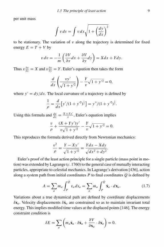
1.3 The principle of least action 9
per unit mass
∫v ds =
∫v dx
√1+
(dy
dx
)2
to be stationary. The variation of v along the trajectory is determined for fixedenergy E = T + V by
v dv = − 1
m
(∂V
∂xdx + ∂V
∂ydy
)= Xdx + Y dy.
Thus v ∂v∂x = X and v ∂v
∂y = Y . Euler’s equation then takes the form
d
dx
(vy ′√
1+ y ′2
)− Y
v
√1+ y ′2 = 0,
where y ′ = dy/dx . The local curvature of a trajectory is defined by
1
ρ= d
dx
[y ′/(1+ y ′2)
12] = y ′′/(1+ y ′2)
32 .
Using this formula and dvdx = X + Y y ′
v, Euler’s equation implies
v
ρ+ (X + Y y ′)y ′
v√
1+ y ′2− Y
v
√1+ y ′2 = 0.
This reproduces the formula derived directly from Newtonian mechanics:
v2
ρ= Y − X y ′√
1+ y ′2= Y dx − Xdy√
dx2 + dy2.
Euler’s proof of the least action principle for a single particle (mass point in mo-tion) was extended by Lagrange (c. 1760) to the general case of mutually interactingparticles, appropriate to celestial mechanics. In Lagrange’s derivation [436], actionalong a system path from initial coordinates P to final coordinates Q is defined by
A =∑
a
ma
∫ Q
Pva dsa =
∑a
ma
∫ Q
Pxa · d xa. (1.7)
Variations about a true dynamical path are defined by coordinate displacementsδxa . Velocity displacements δxa are constrained so as to maintain invariant totalenergy. This implies modified time values at the displaced points [146]. The energyconstraint condition is
δE =∑
a
(ma xa · δxa + ∂V
∂xa· δxa
)= 0.

10 1 History of variational theory
The induced variation of action is
δA =∑
a
ma
∫ Q
P(xa · dδxa + δxa · dxa)
=∑
a
ma xa · δxa|QP −∑
a
ma
∫ Q
P(dxa · δxa − xadt · δxa),
on integrating by parts and using dxa = xadt . The final term here can be replaced,using the energy constraint condition. Then, using dxa = xadt ,
δA =∑
a
ma xa · δxa|QP −∑
a
∫ Q
P
(ma xa + ∂V
∂xa
)· δxadt.
If the end-points are fixed, the integrated term vanishes, and A is stationary ifand only if the final integral vanishes. Since δxa is arbitrary, the integrand mustvanish, which is Newton’s law of motion. Hence Lagrange’s derivation proves thatthe principle of least action is equivalent to Newtonian mechanics if energy isconserved and end-point coordinates are specified.

2
Classical mechanics
The principal references for this chapter are:
[26] Blanchard, P. and Bruning, E. (1992). Variational Methods in MathematicalPhysics: A Unified Approach (Springer-Verlag, Berlin).
[146] Goldstein, H. (1983). Classical Mechanics, 2nd edition (Wiley, New York).[187] Jeffreys, H. and Jeffreys, B.S. (1956). Methods of Mathematical Physics,
3rd edition (Cambridge University Press, New York).[208] Kuperschmidt, B.A. (1990). The Variational Principles of Dynamics (World
Scientific, New York).[210] Lanczos, C. (1966). Variational Principles of Mechanics (University of Toronto
Press, Toronto).[240] Mercier, A. (1959). Analytical and Canonical Formalism in Physics (Interscience,
New York).[323] Pauli, W. (1958). Theory of Relativity, tr. G. Field (Pergamon Press, New York).[393] Synge, J.L. (1956). Relativity: the Special Theory (Interscience, New York).[436] Yourgrau, W. and Mandelstam, S. (1968). Variational Principles in Dynamics and
Quantum Theory, 3rd edition (Dover, New York).
2.1 Lagrangian formalism
Newton’s equations of motion, stated as “force equals mass times acceleration”,are strictly true only for mass points in Cartesian coordinates. Many problems ofclassical mechanics, such as the rotation of a solid, cannot easily be described insuch terms. Lagrange extended Newtonian mechanics to an essentially completenonrelativistic theory by introducing generalized coordinates q and generalizedforces Q such that the work done in a dynamical process is
∑k Qkdqk [436]. Since
this must be the same when expressed in Cartesian coordinates, it follows thatQk =
∑a Xa · ∂Xa
∂qk, where the Newtonian force is Xa = − ∂V
∂Xa. Equivalently, if the
potential function is V ({q}) in generalized coordinates, then Qk = − ∂V∂qk
. The New-tonian kinetic energy T = 1
2
∑a ma x2
a defines momenta pa = ∂T∂ xa= ma xa , which
becomes pk = ∂T∂ qk
when kinetic energy is expressed as T ({q, q}). The equationsof motion pa = X transform into pk = Qk . Although this can be shown by direct
11

12 2 Classical mechanics
transformation, a more elegant and ultimately more general procedure is to provethe variational principle of Hamilton in a form that is valid for any choice of gen-eralized coordinates.
2.1.1 Hamilton’s variational principle
The principle of least action suffers from the awkward constraint that energy must befixed on nonphysical displaced trajectories. Following the introduction by Lagrangeof a dynamical formalism using generalized coordinates, it was shown by Hamiltonthat a revised variational principle could be based on a new definition of action thathad the full generality of Lagrange’s theory. Hamilton’s definition of the actionintegral is
I =∫ t1
t0
L dt, (2.1)
where the Lagrangian L is an explicit function of generalized coordinates {q} andtheir time derivatives {q},
L = T (q, q)− V (q, q). (2.2)
Generalized momenta are defined by pk = ∂L∂ qk
and generalized forces are definedby Qk = ∂L
∂qk. When applied using t as the independent variable, Euler’s variational
equation for the action integral I takes the form of Lagrange’s equations of motion
d
dt
∂L
∂q− ∂L
∂q= 0. (2.3)
Hamilton considered variations δq(t) that define continuous generalized trajectorieswith fixed end-points, q(t0) = q0 and q(t1) = q1. The variational expression is
δ I =∫ t1
t0
dt
{δq(t)
∂L
∂q+ δq(t)
∂L
∂q
}= 0.
Following the logic of Euler, after integrating by parts to replace the term in δq byone in δq , this implies the Lagrangian equations of motion.
2.1.2 Dissipative forces
Hamilton’s principle exploits the power of generalized coordinates in problems withstatic or dynamical constraints. Going beyond the principle of least action, it can alsotreat dissipative forces, not being restricted to conservative systems. If energy loss

2.1 Lagrangian formalism 13
during system motion due to a nonconservative force is −dW , where dW =∑k Qkdqk , then a dissipative action function is defined by its variation δ I =∫ t1
t0(δL + δW )dt . Hamilton’s variational principle implies modified equations of
motion
d
dt
∂L
∂qk− ∂L
∂qk= Qk .
The dissipative term takes the form of a nonconservative force, Qk , acting on thegeneralized coordinate qk .
2.1.3 Lagrange multiplier method for constraints
The differential form d X j =∑
k ak j dqk + akt dt = 0 defines a general linearconstraint condition. For an integrable or holonomic constraint, expressed byX j ({qk}, t) = 0, the coefficients are partial derivatives of X j such that akj = ∂X j
∂qk
and akt = ∂X j
∂t . Nonintegrable or nonholonomic constraints are defined by the differ-ential form. In applications of Hamilton’s principle, δX j differs from d X j becausethe displacement of each point on a trajectory is defined such that δt = 0. Hencethe coefficients akt drop out of δX j .
Lagrange introduced the very powerful method of Lagrange multipliers to incor-porate such constraints into the formalism of analytical dynamics. The basic ideais that if a term X jλ j is added to L , its gradients provide a generalized internalforce that dynamically enforces the desired constraint. The Lagrange multiplierλ j provides a generalized coordinate whose value is to be determined so that theconstraint condition is satisfied. This artificial coordinate characterizes an effectivepotential well whose extremum stabilizes a system conformation that satisfies theconstraint condition. Because the added term X jλ j vanishes when the constraintcondition is satisfied, it does not change any physical properties of the system exceptby avoiding dynamical states incompatible with the constraint.
The equations of motion, generalized to include holonomic or nonholonomicconstraints with Lagrange multipliers, are
d
dt
∂L
∂qk− ∂L
∂qk−∑
j
ak jλ j = 0.
These equations are to be supplemented by the alternative constraint conditions:
X j ({qk}, t) = 0,∑k
ak j qk + akt = 0,

14 2 Classical mechanics
for holonomic and nonholonomic constraints, respectively. The number of equa-tions equals the number of unknown quantities {qk, λ j } in either case. Forces ofconstraint Qk =
∑j ak jλ j appear in the modified Lagrange equations.
A simple example of the use of Lagrange multipliers is a hoop of mass Mand radius r rolling without slipping down an inclined plane [146]. Appropri-ate generalized coordinates are x , the distance from the top of the plane to thepoint of contact and θ , the angle of rotation of the hoop. If the plane is ata fixed angle φ from the horizontal, kinetic and potential energy are, respec-tively, T = 1
2 Mx2 + 12 Mr2θ
2, V = −Mgx sinφ subject to the differential con-
straint d X = rdθ − dx = 0. δ(T − V + Xλ) replaces δL , where λ is the Lagrangemultiplier for the constraint. The coefficients in the differential constraint form areaθ = r and ax = −1. The equations of motion and constraint are
Mx − Mg sinφ + λ = 0,
Mr2θ − λr = 0,
r θ − x = 0.
The solution is simplified because r θ = x implies Mx = λ, so that x = g sinφ/2.Hence λ = Mg sinφ/2, and −λ is the translational force of constraint. The angu-lar acceleration is θ = g sinφ/2r . The hoop rolls with half the unconstrainedtranslational acceleration.
2.2 Hamiltonian formalism
Generalizing Newton’s equations of motion, Lagrange’s equations also set the timerate of change of momenta p equal to forces Q. Hamilton recognized that thesegeneralized momenta could replace the time derivatives q as fundamental variablesof the theory. This is most directly accomplished by a Legendre transformation, asdescribed in the following subsection.
2.2.1 The Legendre transformation
Given F(x, y) such that
d F = u(x, y) dx + v(x, y) dy = ∂F
∂xdx + ∂F
∂ydy,
it is often desirable to transform to different independent variables (u, y). Thealternative function G(u, y) = F(x, y)− ux characterizes a Legendre trans-formation, such that dG = d F − u dx − x du = v dy − x du. Thus the partial
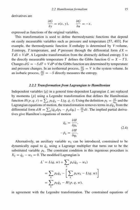
2.2 Hamiltonian formalism 15
derivatives are
∂G
∂y= v(x, y),
∂G
∂u= −x,
expressed as functions of the original variables.This transformation is used to define thermodynamic functions that depend
on easily measurable variables such as pressure and temperature [57, 403]. Forexample, the thermodynamic function X :enthalpy is determined by V :volume,S:entropy, T :temperature, and P:pressure through the differential form d X =T dS+ V dP. A Legendre transformation from the abstractly defined entropy S tothe directly measurable temperature T defines the Gibbs function G = X − T S.Changes dG = −S dT+ V dP of the Gibbs function are determined by temperatureand pressure changes. In an isothermal process, ∂G
∂P = V is the system volume. Inan isobaric process, ∂G
∂T = −S directly measures the entropy.
2.2.2 Transformation from Lagrangian to Hamiltonian
Independent variables {q} in a general time-dependent Lagrangian L are replacedby momenta {p} using a Legendre transformation that defines the Hamiltonianfunction H (p, q, t) =∑
k pkqk − L(q, q, t). Using the definition pk = ∂L∂ qk
and theLagrangian equations of motion, the transformation removes terms in dqk from thedifferential form d H =∑
k{qkdpk − pkdqk} − ∂L∂t dt . The implied partial deriva-
tives give Hamilton’s equations of motion
qk =∂H
∂pk,
(2.4)
− pk =∂H
∂qk.
Alternatively, an auxiliary variable wk can be introduced, constrained to bedynamically equal to qk using a Lagrange multiplier that turns out to be thesubstituted variable pk . The constraint condition in this ingenious procedure isXk = qk − wk = 0. The modified Lagrangian is
L ′ = L(q, w)+∑
k
pk(qk − wk)
=∑
k
pkqk −[∑
k
pkwk − L(q, w)
]
=∑
k
pkqk − H (p, q, w),
in agreement with the Legendre transformation. The constrained equations of

16 2 Classical mechanics
motion are
∂L ′
∂pk= qk − wk = qk −
∂H
∂pk= 0;
d
dt
∂L ′
∂qk− ∂L ′
∂qk= pk +
∂H
∂qk= 0;
∂L ′
∂wk= ∂L
∂wk− pk = − ∂H
∂wk= 0.
The first and second of these equations are Hamilton’s equations of motion. Thefirst and third establishwk = qk and pk = ∂L
∂wkas dynamical conditions, equivalent
to pk = ∂L∂ qk
.
2.2.3 Example: the central force problem
In spherical polar coordinates, for one mass point moving in a central potentialV = V (r ),
T = 1
2m(r2 + r2θ
2).
The Hamiltonian is H = p2r
2m +p2θ
2mr2 + V (r ), where pr = ∂T∂ r = mr , and pθ = ∂T
∂θ=
mr2θ . Using the relevant partial derivatives, Hamilton’s equations of motion are
pθ = 0; θ = pθmr2
;
pr = mr θ2 − ∂V
∂r; r = pr
m.
For specified energy E and angular momentum pθ = const = �, on solving H = Efor pr ,
mr = pr = [2m(E − V (r ))− �2/r2]12 .
A trajectory r (t) is obtained by integrating r between turning points, where theargument of the square root vanishes. Using dθ = �
mr2drr , this formula for r provides
an equation to be integrated for a classical orbit,
dθ
dr= �
r2[2m(E − V (r ))− �2/r2]−
12 .

2.3 Conservation laws 17
2.3 Conservation laws
Conservation of energy follows directly from Hamilton’s equations. The differentialchange of the Hamiltonian along a trajectory is
d H =∑
k
(qkdpk − pkdqk)+ ∂H
∂tdt,
using the Hamiltonian equations of motion. The total time derivative is
d H
dt=∑
i
(qk pk − pk qk)+ ∂H
∂t= ∂H
∂t.
Hence, stated as a theorem,
∂H
∂t= 0 ⇒ H (t) = E = const,
and energy is conserved unless H is explicitly time-dependent.Since Hamilton’s equations imply that pk = 0 if ∂H
∂qk= 0, pk is a constant of
motion if qk is such an ignorable coordinate. An ingenious choice of generalizedcoordinates can produce such constants and simplify the numerical or analytic taskof integrating the equations of motion.
The close connection between symmetry transformations and conservation lawswas first noted by Jacobi, and later formulated as Noether’s theorem: invarianceof the Lagrangian under a one-parameter transformation implies the existence of aconserved quantity associated with the generator of the transformation [304]. Theequations of motion imply that the time derivative of any function �(p, q) is
� =∑
k
(∂�
∂qkqk +
∂�
∂pkpk
)=∑
k
(∂�
∂qk
∂H
∂pk− ∂�∂pk
∂H
∂qk
),
which defines a classical Poisson bracket {�, H}. A constant of motion is charac-terized by {�, H} = 0. Invariance under a symmetry transformation implies sucha vanishing Poisson bracket for the symmetry generator.
By Noether’s theorem, invariance of the Lagrangian under an infinitesimal timedisplacement implies conservation of energy. This is consistent with the direct proofof energy conservation given above, when L and by implication H have no explicittime dependence. Define a continuous time displacement by the transformation t =t ′ + α(t ′) whereα(t0) = α(t1) = 0, subject toα→ 0. Time intervals on the originaland displaced trajectories are related by dt = (1+ α′)dt ′ or dt ′ = (1− α′)dt . Thetransformed Lagrangian is
L(q, q) = L(q, q ′(1− α′)) = L(q, q ′)−∑
k
∂L
∂ qkqkα
′.

18 2 Classical mechanics
The transformed action integral is
Iα =∫ t1
t0
L(q, q) dt =∫ t1
t0
L(q, q ′(1− α′))(1+ α′) dt ′.
In the limit α→ 0 this is
Iα→0 = I −∫ t1
t0
(∑k
∂L
∂qkqk − L
)α′dt ′.
Treating α as a generalized coordinate, its equation of motion is
d
dt ′∂L ′
∂α′= − d
dt ′
(∑k
pkqk − L
)= 0,
so that H =∑k pkqk − L = const = E .
Similarly for translational invariance, an infinitesimal coordinate translation isdefined for a single particle by
x′i = xi +α(t), α→ 0.
Assuming invariant potential energy, the transformed kinetic energy is
Tα = 1
2
∑i
mi (xi + α)2 = T +∑
i
mi xi · α+ O(α2).
Treating the components of α as generalized coordinates, an equation of motion isimplied in the form
∂Lα∂α
=∑
i
mi xi = const = P,
the conservation law for linear momentum.
2.4 Jacobi’s principle
As an introduction to relativistic dynamics, it is of interest to treat time as a dy-namical variable rather than as a special system parameter distinct from particlecoordinates. Introducing a generic global parameter τ that increases along anygeneralized system trajectory, the function t(τ ) becomes a dynamical variable. Inspecial relativity, this immediately generalizes to ti (τ ) for each independent particle,associated with spatial coordinates xi (τ ). Hamilton’s action integral becomes
I =∫
Lt ′dτ, (2.5)

2.4 Jacobi’s principle 19
where t ′ = dt/dτ . Limiting the discussion to conservative systems, with fixedenergy E , the modified Lagrangian Lt ′ does not depend on t . Hence the generalizedmomentum pt = ∂
∂t ′ (Lt ′) is a constant of motion. In detail,
pt = L +∑
i
∂L
∂q it ′∂
∂t ′
(q ′it ′
)= L −
∑i
pi q i = −H = −E .
Again anticipating relativistic dynamics, energy is related to momenta as time isrelated to spatial coordinates.
Since time here is an “ignorable” variable, it can be eliminated from the dynamicsby subtracting pt t ′ from the modified Lagrangian and by solving H = E for t ′ asa function of the spatial coordinates and momenta. This produces Jacobi’s versionof the principle of least action as a dynamical theory of trajectories, from whichtime dependence has been removed. The modified Lagrangian is
� = Lt ′ − pt t′ = (T − V + E )t ′ = 2T t ′,
such that
∂
∂t ′� = ∂
∂t ′(Lt ′)− pt = 0.
Since kinetic energy is positive, the action integral A = ∫2T t ′dτ is nondecreas-
ing. This suggests using a global parameter τ = s defined by the Riemannian lineelement
ds2 =∑i, j
mi j dqi dq j ,
where the positive-definite matrix mi j defines a mass tensor as a function of gener-alized coordinates. Then
s2 =∑i, j
mi j q i q j = 2T .
This makes it possible to express t ′ as a function of the generalized coordinates andmomenta. s2 = (s ′/t ′)2 = 2T implies that ds = (2T )
12 dt , or t ′ = (2T )−
12 s ′. The
reduced action integral, originally derived by Jacobi, is
A =∫
2T t ′dτ =∫
(2T )12 s ′dτ =
∫(2T )
12 ds.
Because variations are restricted to those that conserve energy, 2T = 2(E − V ) andds = (2(E − V ))
12 dt along the varied trajectories. The action integral becomes
A =∫
2(E − V )dt =∫ ∑
i, j
mi j q i q j dt =∫ ∑
i
pi dqi .

20 2 Classical mechanics
δA = 0 subject to the energy constraint restates the principle of least action. Whenthe external potential function is constant, the definition of ds as a path elementimplies that the system trajectory is a geodesic in the Riemann space defined bythe mass tensor mi j . This anticipates the profound geometrization of dynamicsintroduced by Einstein in the general theory of relativity.
2.5 Special relativity
The concept of a mass point remains valid, but a time interval dt can no longerbe treated as a nondynamical parameter. Einstein’s basic postulate [323, 393] isthat the interval ds between two space-time events is characterized by the invariantexpression
ds2 = c2dt2 − dx2 − dy2 − dz2,
where c is the constant speed of light. The space and time intervals can be measuredin any reference frame in uniform linear motion, referred to as an inertial frame.Space and time intervals measured in two such inertial frames are related by alinear Lorentz transformation, parametrized by the velocity and direction of relativemotion. It is convenient to introduce Minkowski space-time coordinates
dxµ = (dx1, dx2, dx3, dx4) = (dx, dy, dz, ic dt),
such that ds2 = −dxµdxµ, using the summation convention of Einstein. A covariant4-vector Aµ is defined by four quantities that are related by the appropriate Lorentztransformation when measured in two different inertial frames.
Since dt cannot be singled out for special treatment, the covariant generalizationof Hamilton’s variational principle for a single particle requires an invariant actionintegral
I =∫�(xµ, uµ, τ ) dτ,
where c2dτ 2 = ds2 > 0 for a timelike interval defines an invariant proper timeinterval dτ . uµ = dxµ/dτ defines a covariant velocity 4-vector. The variationalcondition δ I = 0, for fixed end-points x0
µ and x1µ separated by a timelike interval,
implies relativistic Lagrangian equations of motion
d
dτ
∂�
∂uµ− ∂�∂xµ
= 0.

2.5 Special relativity 21
2.5.1 Relativistic mechanics of a particle
As measured in some inertial reference frame, the instantaneous particle velocityis v = (dx/dt, dy/dt, dz/dt). It is customary to define noninvariant parametersβ = v/c and γ = (1− β2)−
12 . The definition of the invariant interval ds2 implies
that dτ 2 = dt2(1− β2), where dt is the measured time interval. Hence dtdτ = γ , as
defined above. The spatial components of the 4-velocity are u = γ v and the timecomponent is u4 = iγ c. Hence uµuµ = (v2 − c2)γ 2 = −c2, a space-time invariant.
Unlike classical mechanics, the 4-acceleration is not independent of the 4-velocity. Because uµuµ is invariant, its τ -derivative must vanish, so that
uµduµdτ
= 0.
This implies a relationship between classical velocity and acceleration,
v · d
dt(γ v)− c2 dγ
dt= 0,
which is an immediate consequence of the definition of γ .The variational formalism makes it possible to postulate a relativistic Lagrangian
that is Lorentz invariant and reduces to Newtonian mechanics in the classical limit.Introducing a parameter m, the proper mass of a particle, or mass as measured in itsown instantaneous rest frame, the Lagrangian for a free particle can be postulatedto have the invariant form � = 1
2 muµuµ = − 12 mc2. The canonical momentum is
pµ = muµ and the Lagrangian equation of motion is
d
dτpµ = d
dτ(muµ) = 0,
which clearly reduces to Newton’s equation when β → 0.As measured in an inertial reference frame, the spatial components of the canon-
ical momentum are p = mγ v and the time component is p4 = imγ c. This can berelated to classical quantities by defining the relative energy as E = mγ c2 so thatp4 = i
c E . Thus pµ is an energy–momentum vector, for which pµ pµ = −m2c2, aconstant for unaccelerated motion. In terms of classical quantities, this invariantnorm is expressed by p2 − E2
c2 = −m2c2, or E2 = m2c4 + p2c2, which implies thefamous Einstein formula E = mc2 in the instantaneous rest frame of a particle.In the limit β → 0, E = mc2 + 1
2 mv2 + · · ·, verifying the classical formula forkinetic energy.
The free-particle Lagrangian � is a space-time constant − 12 mc2. If terms are
added that are invariant functions of xµ, the equations of motion become
d
dτpµ = Xµ

22 2 Classical mechanics
defining a covariant Minkowski 4-force Xµ = ∂�∂xµ
. The canonical momenta aremodified if these added terms depend explicitly on the 4-velocity uµ. It can nolonger be assumed that the rest mass is constant.
If m is not constant, the equations of motion are
d
dτ
(m
dxµdτ
)= dm
dτ
dxµdτ
+ md2xµdτ 2
= Xµ.
On multiplying by uµ = dxµ/dτ and summing, and using uµuµ = −c2, whichimplies uµ
ddτ uµ = 0, this reduces to
d
dτ(mc2) = −Xµuµ.
The rest mass remains constant if the 4-force and 4-velocity are orthogonal in theMinkowski sense that Xµuµ = 0.
In relativistic theory, energy is a component of the 4-momentum, and is conservedonly under particular circumstances. Given d
dτ = γ ddt , the equation of motion for
p4 = i E/c is
γd
dt(i E/c) = X4.
Consider a 4-force Xµ that does not change the rest mass m. As shown above,Xµuµ = iγ cX4 + γX · v = 0, since u4 = iγ c and u = γ v. Then X4 = i
c X · v forsuch a force, and
γd
dtE = X · v.
2.5.2 Relativistic motion in an electromagnetic field
The classical electromagnetic force acting on a particle of charge q is the Lorentzforce (in Gaussian units)
Q = q
{E + 1
c(v ×B)
},
where, in terms of scalar and vector potentials φ,A,
B =∇ × A, E = −∇φ − 1
c
∂A∂t.
After expanding the triple vector product v × ∇ × A = v ×B,
Q = q
c
{∂
∂x(A · v− φc)− d
dtA}. (2.6)

2.5 Special relativity 23
This is of the form
Q = ∂W
∂x− d
dt
∂W
∂v,
where W = qc (A · v− φc).
Given the electromagnetic 4-vector field Aµ = (A, iφ) and the 4-velocity uµ =(γ v, iγ c), W is the classical limit of a relativistic invariant γW = q
c Aµuµ. Thisterm augments the free-particle relativistic Lagrangian to give
� = 1
2muµuµ + q
cAµuµ. (2.7)
The canonical momentum is pµ = muµ + qc Aµ. If defined such that p4 = i
c E ,the energy is E = mc2γ + qφ, adding electrostatic energy to rest energy mc2 andrelativistic kinetic energy T = mc2(γ − 1). Because muµmuµ = (p − q
c A)µ(p −qc A)µ = −m2c2, energy and momentum are related by (p− q
c A)2 − (mc2 +T )2/c2 = −m2c2, or
(mc2 + T )2 =(
p− q
cA)2
c2 + m2c4.
Written as a formula for iteration, this is
T =(
p− q
cA)2/
(2m + T/c2).
The Lagrangian equations of motion are
d
dτ
(muµ + q
cAµ)= q
c
∂
∂xµ(Aνuν).
Using ddτ = γ d
dt , these equations can be written as
γd
dt(muµ) = Xµ = q
c
{∂
∂xµ(Aνuν)− γ d
dtAµ
}. (2.8)
Comparing the classical force Q, given above, the spatial components of Xµ areX = γQ, verifying the historical fact that Maxwell’s theory is covariant underLorentz transformations.


3
Applied mathematics
The principal references for this chapter are:
[77] Dennis, J.E. and Schnabel, R.B. (1983). Numerical Methods for UnconstrainedOptimization and Nonlinear Equations (Prentice-Hall, Englewood Cliffs,New Jersey).
[125] Fletcher, R. (1987). Practical Methods of Optimization, 2nd edition (Wiley,New York).
[168] Hestenes, M.R. (1966). Calculus of Variations and Optimal Control Theory(Wiley, New York).
[332] Pulay, P. (1987). Analytical derivative methods in quantum chemistry, Adv. Chem.Phys. 69, 241–286.
[439] Zerner, M.C. (1989). Analytic derivative methods and geometry optimization, inModern Quantum Chemistry, eds. A. Szabo and N.S. Ostlund (McGraw-Hill,New York), pp. 437–458.
Before undertaking the major subject of variational principles in quantum mech-anics, the present chapter is intended as a brief introduction to the extension ofvariational theory to linear dynamical systems and to classical optimization meth-ods. References given above and in the Bibliography will be of interest to the readerwho wishes to pursue this subject in fields outside the context of contemporary theor-etical physics and chemistry. The specialized subject of optimization of moleculargeometries in theoretical chemistry is treated here in some detail.
3.1 Linear systems
Any multicomponent system whose dynamical behavior is governed by coupledlinear equations can be modelled by an effective Lagrangian, quadratic in the sys-tem variables. Hamilton’s variational principle is postulated to determine the timebehavior of the system. A dynamical model of some system of interest is valid if itsatisfies the same system of coupled equations. This makes it possible, for example,
25

26 3 Applied mathematics
to construct an electrical circuit model of a mechanical system, or to reduce eitherto a computer model with the appropriate choice of parameters.
For example [146], a system of interconnected electrical circuits and a mechanicalsystem of masses connected by springs satisfy the same linear equations if systemparameters are related by the following definitions:
Symbol Electrical circuit Masses on springs
I current displacementM inductance reciprocal mass tensorR resistance viscous forceC capacitance inverse spring constantE external emf driving force
The Lagrangian for this linear system is
L = 1
2
∑j,k
M jk I j I k − 1
2
∑j
1
C jI 2
j +∑
j
E j (t)I j .
A dissipation function adds a nonintegrable term
δW = −∑
j
R j I jδ I j
to δL . The implied equations of motion are∑k
M jk I k + R j I j + I j/C j = E j (t).
3.2 Simplex interpolation
In many practical applications of nonlinear optimization, a linear approximationis iterated until some vector of system parameters has negligible norm. At eachstage of such a process, previous steps provide a set of m ≤ n trial vectors in ann-dimensional parameter space, each associated with an output vector of gradientsof the quantity to be optimized. The next iterative step is facilitated if a linear com-bination of such vectors can be found that produces an output vector of minimumnorm.
Linear interpolation can be described geometrically in terms of an m-simplex inthe n-dimensional parameter space. An m-simplex in a hyperspace of dimensionn ≥ m is a set of m + 1 points that do not lie in a subspace of dimension lessthan m. For example, a triangle is a 2-simplex and a tetrahedron is a 3-simplex.The interior of a simplex is the set of points X =∑
i xiλi , such that 0 ≤ λi ≤ 1 and∑i λi = 1.
3.2 Simplex interpolation 27
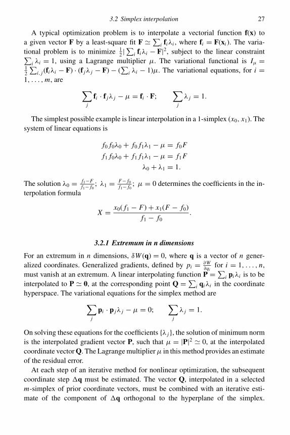
A typical optimization problem is to interpolate a vectorial function f(x) toa given vector F by a least-square fit F �∑
i fiλi , where fi = F(xi ). The varia-tional problem is to minimize 1
2 |∑
i fiλi − F|2, subject to the linear constraint∑i λi = 1, using a Lagrange multiplier µ. The variational functional is Iµ =
12
∑i, j (fiλi − F) · (f jλ j − F)− (
∑i λi − 1)µ. The variational equations, for i =
1, . . . ,m, are ∑j
fi · f jλ j − µ = fi · F;∑
j
λ j = 1.
The simplest possible example is linear interpolation in a 1-simplex (x0, x1). Thesystem of linear equations is
f0 f0λ0 + f0 f1λ1 − µ = f0 F
f1 f0λ0 + f1 f1λ1 − µ = f1 F
λ0 + λ1 = 1.
The solution λ0 = f1−Ff1− f0
; λ1 = F− f0
f1− f0; µ = 0 determines the coefficients in the in-
terpolation formula
X = x0( f1 − F)+ x1(F − f0)
f1 − f0.
3.2.1 Extremum in n dimensions
For an extremum in n dimensions, δW (q) = 0, where q is a vector of n gener-alized coordinates. Generalized gradients, defined by pi = ∂W
∂qifor i = 1, . . . , n,
must vanish at an extremum. A linear interpolating function P =∑i piλi is to be
interpolated to P � 0, at the corresponding point Q =∑i qiλi in the coordinate
hyperspace. The variational equations for the simplex method are∑j
pi · p jλ j − µ = 0;∑
j
λ j = 1.
On solving these equations for the coefficients {λ j }, the solution of minimum normis the interpolated gradient vector P, such that µ = |P|2 � 0, at the interpolatedcoordinate vector Q. The Lagrange multiplierµ in this method provides an estimateof the residual error.
At each step of an iterative method for nonlinear optimization, the subsequentcoordinate step �q must be estimated. The vector Q, interpolated in a selectedm-simplex of prior coordinate vectors, must be combined with an iterative esti-mate of the component of �q orthogonal to the hyperplane of the simplex.

28 3 Applied mathematics
A Hessian matrix
Fi j = ∂2W
∂qi∂q j,
is defined by small displacements about a given point, such that �p = F�q. Ageneralization of Newton’s method can be used to estimate the location of a zerovalue of a vector from its given value and derivative. If an approximation to F−1 ismaintained and updated at each iterative step, then
�q = �q⊥ +∑
i
qiλi ,
where
�q⊥ = −F−1p+∑
i, j≤m
(F−1p · qi )[(q · q)]−1i j q j .
Alternatively, the interpolation and extrapolation steps can be combined, using theformula [75]
q = Q− F−1P =∑
i
(qi − F−1pi )λi .
3.3 Iterative update of the Hessian matrix
Quadratic expansion of a function W (q) about a local extremum takes the form
W � W 0 + 1
2
∑i, j
F 0i, j�qi�q j .
At a general point, displaced from the extremum, gradients pi = ∂W∂qi
do not vanish.
Newton’s formula estimates a displacement toward the extremum �q = −Gp0,where G is the inverse of the Hessian matrix F. Since F is not constant in a nonlinearproblem, if it cannot be computed directly it must be deduced from an initialestimate followed by iterative updates. In many circumstances, the gradients at ageneral point can be computed directly or estimated with useful accuracy. Theneach successive coordinate increment �q is associated with a gradient increment�p. If the Hessian matrix is known, F�q = �p for sufficiently small increments.Given an estimated F 0, it must in general be updated to be consistent with thecomputed gradient increment�p. This implies a linear formula for the increment ofF ,�F�q = �p− F 0�q. Since this provides only n equations for the n2 elementsof�F , the incremental matrix cannot be determined from data obtained in a singleiterative step.
The practical problem is to find a way to use the information obtained in eachiterative step without making unjustified changes of the Hessian. This could be

3.3 Iterative update of the Hessian matrix 29
accomplished if the Hessian were projected onto two orthogonal subspaces, one ofwhich corresponds to a subset of m linearly independent increments �q and thecorresponding �p. A rank-m (Rm) update in the vector space spanned by thesecoordinate increments is defined such that�q†�F�q = �q†(�p− F 0�q). Thiscondition is satisfied by
�F(Rm) = �p(�q†�p)−1�q†(�p− F 0�q)(�p†�q)−1�p†.
Alternatively, the inverse matrix G can be updated directly,
�G(Rm) = �q(�p†�q)−1�p†(�q− G0�p)(�q†�p)−1�q†.
These formulas update the rank-m projection of F 0 or G0, using the nonhermitianprojection operator Pm = �p(�q†�p)−1�q†, such that P†
m�q = �q, Pm�p =�p, and PmPm = Pm . This operator projects onto the m-dimensional vector spacespanned by the specified set of gradient vectors. The Rm update has the undesirableproperty of altering the complementary projection of the updated matrix.
3.3.1 The BFGS algorithm
The BFGS (Broyden [42], Fletcher [124], Goldfarb [145], Shanno [379]) algor-ithm is an update procedure for the Hessian matrix that is widely used in iterativeoptimization [125]. The simpler Rm update takes the form
F = �Fmm + F 0 − Pm F 0P†m,
where �Fmm�q = �p. Replacing this by a form that leaves the complementaryprojection of F 0 unchanged,
F = �Fmm + (I − Pm)F 0(I − P†m),
the BFGS update of F 0 is
�F(BFGS) = �p(�q†�p)−1�q†(�p+ F 0�q) (�p†�q)−1�p†
−�p(�q†�p)−1�q†F 0 − F 0�q(�p†�q)−1�p†.
Alternatively, the BFGS update of G0 is
�G(BFGS) = �q(�p†�q)−1�p†(�q+ G0�p) (�q†�p)−1�q†
−�q(�p†�q)−1�p†G0 − G0�p(�q†�p)−1�q†.
For exact infinitesimal increments, the matrix
dp†dq = dq†dp = dq†F dq

30 3 Applied mathematics
is symmetric and nonsingular at an extremum of W . When m > 1, the matrices�p†�q and�q†�p are not necessarily symmetric or even nonsingular when eval-uated with approximate gradients away from an extremum. Any practical algorithmmust modify these matrices to remove singularities.
3.4 Geometry optimization for molecules
Quantum mechanical calculations of the electronic structure of molecules for fixednuclear coordinates involve lengthy calculations even using the sophisticated com-putational methods that have evolved over half a century of computational quantumchemistry. A principal output of such calculations is the variational energy as a func-tion of the nuclear coordinates. Current methodology makes it possible to computethe energy gradients or effective forces as well as the energy itself. For chemicalapplications, equilibrium geometries and the coordinates of transition states mustbe deduced from such data [357, 332, 439].
For such applications of classical optimization theory, the data on energy andgradients are so computationally expensive that only the most efficient optimizationmethods can be considered, no matter how elaborate. The number of quantumchemical wave function calculations must absolutely be minimized for overallefficiency. The computational cost of an update algorithm is always negligiblein this context. Data from successive iterative steps should be saved, then used toreduce the total number of steps. Any algorithm dependent on line searches in theparameter hyperspace should be avoided.
Molecular geometry can be specified either in Cartesian coordinates xa for each ofN nuclei, or in generalized internal coordinates qk , where k = 1, . . . , 3N − 6 for ageneral polyatomic molecule. Neglecting kinetic energy of nuclear motion becauseof the large nuclear masses, six generalized coordinates corresponding to translationand rotation are subject to no internal forces, and can be fixed or removed from theinternal coordinates considered in geometry optimization. Cartesian coordinates aresubject to six constraint conditions, which may be imposed directly or indirectlyusing Lagrange multipliers. This number reduces to five for a linear molecule, sincerotation about the molecular axis is not defined.
An equilibrium state is defined for generalized coordinates such that the totalenergy E({q}) is minimized. The energy gradients p = ∂E
∂q are forces with reversedsign. Coordinate and gradient displacements from m successive iterations are savedas m × n column matrices,�qk and�pk , respectively. The Hessian matrix is Fi j =∂2 E∂qi∂q j
, such that Newton’s extrapolation formula is�q = −Gp0, where G = F−1.In quasi-Newton methods, a parametrized estimate of F or G is used initially,
then updated at each iterative step. Saved values of q, p can be used in standardalgorithms such as BFGS, described above.

3.4 Geometry optimization for molecules 31
3.4.1 The GDIIS algorithm
This method [75] uses simplex interpolation combined with an update step such asBFGS. The variational functional is
Iµ = 1
2
∣∣∣∣∣m∑
k=0
pkck
∣∣∣∣∣2
−(
m∑k=0
ck − 1
)µ.
The variational equations determined by δ Iµ = 0 are∑j
pk · p j c j − µ = 0;∑
j
c j = 1.
The interpolated gradient vector is p =∑k pkck and the interpolated coordinate
vector is q =∑k qkck . In the GDIIS algorithm, a currently updated estimate of the
inverse Hessian is used to estimate a coordinate step based on these interpolatedvectors. This gives
�q = qupd − q = −(G0 +�G)p
or, equivalently, with G = G0 +�G,
qupd = q− Gp =∑
k
(qk − Gpk)ck .
In test calculations [75] this algorithm was found to produce rapid convergence.When combined with single-step (m = 1) BFGS update of the inverse Hessian, thisis a very efficient algorithm.
The GDIIS algorithm can locate saddle points (transition states), because itsearches specifically for a point at which all gradients vanish, independently ofthe sign of the second derivative. A reaction path can be followed by selecting theeigenvector of G that belongs to the eigenvalue of greatest magnitude [332].
3.4.2 The BERNY algorithm
This algorithm, standard in the widely used GAUSSIAN program system, is arank-m update of the Hessian matrix, in an orthonormal basis [356]. A basis of unitvectors is constructed in the m-dimensional vector space spanned by the increments�q. For k = 1,m, define
dk = �qk −k−1∑j=1
e j (e j ·�qk).
Then orthonormal unit vectors are constructed such that
ek = dk(dk · dk)−12 .

32 3 Applied mathematics
A significant advantage of this procedure is that nearly linearly dependent vectorscan be eliminated at this stage, simply reducing the value of m. The resulting unitvectors define an n × m column matrix. Using these unit vectors, the algorithmsolves an m × m system of linear equations in the e-space,
(�q†e)(e† Fe) = (�p†e).
The matrix (�q†e) is lower-triangular by construction. For the index range j≤ i≤m,solution matrix elements are determined by
(ei† Fe j ) = (�qi†ei )−1
[(�pi†e j )−
i−1∑k=1
(�qi†ek)(ek† Fe j )
].
The Hessian matrix F 0 +�F is updated and symmetrized, using
�F =∑i, j
ei [(ei† Fe j ) j≤i + (e j† Fei ) j>i − (ei†F 0e j )]e j†.
Several aspects of the BERNY algorithm have a somewhat inconsistent math-ematical basis. A modified algorithm may be more efficient. The Hessian matrixcan be constructed directly from gradient vectors but not from coordinate vectors.The defining relation F�q = �p implies that an Hermitian matrix F must havethe form �pA�p†. In principle, the unit vectors of the BERNY algorithm shouldbe in the �p space. However, the orthonormalization process ensures numericalstability by systematizing rejection of redundant coordinate increments �q. Onemight then propose an alternative algorithm, in which this basis is used to updatethe inverse Hessian G. Because G�p = �q, this matrix has the formal expansion�qB�q†. The equations to be solved are
(�p†e)(e†Ge) = (�q†e).
In these equations, the matrix (�p†e) is no longer triangular. However, the additionalcomputational effort may be unimportant if the number of iterative steps can bereduced, thus saving energy and gradient evaluations. The matrix e†Ge is to besymmetrized before updating G. The incremental matrix is
�G =∑i, j
ei
[1
2(ei†Ge j )+ 1
2(e j†Gei )− (ei†G0e j )
]e j†.

II
Bound states in quantum mechanics
This part introduces variational principles relevant to the quantum mech-anics of bound stationary states. Chapter 4 covers well-known varia-tional theory that underlies modern computational methodology for elec-tronic states of atoms and molecules. Extension to condensed matter isdeferred until Part III, since continuum theory is part of the formal basis ofthe multiple scattering theory that has been developed for applications inthis subfield. Chapter 5 develops the variational theory that underliesindependent-electron models, now widely used to transcend the practicallimitations of direct variational methods for large systems. This is ex-tended in Chapter 6 to time-dependent variational theory in the contextof independent-electron models, including linear-response theory and itsrelationship to excitation energies.

4
Time-independent quantum mechanics
The principal references for this chapter are:
[74] Courant, R. and Hilbert, D. (1953). Methods of Mathematical Physics (Interscience,New York).
[101] Epstein, S.T. (1974). The Variation Method in Quantum Chemistry (AcademicPress, New York).
[180] Hurley, A.C. (1976). Electron Correlation in Small Molecules (Academic Press,New York).
[242] Merzbacher, E. (1961). Quantum Mechanics (Wiley, New York).[365] Schrodinger, E. (1926). Quantisiering als Eigenwertproblem, Ann. der Physik 81,
109–139.[394] Szabo, A. and Ostlund, N. S. (1982). Modern Quantum Chemistry; Introduction to
Advanced Electronic Structure Theory (McGraw-Hill, New York).
In 1926, Schrodinger [365] recognized that the variational theory of elliptical differ-ential equations with fixed boundary conditions could produce a discrete eigenvaluespectrum in agreement with the energy levels of Bohr’s model of the hydrogen atom.This conceptually startling amalgam of classical ideas of particle and field turnedout to be correct. Within a few years, the new wave mechanics almost completelyreplaced the ad hoc quantization of classical mechanics that characterized the “old”quantum theory initiated by Bohr. Although the matrix mechanics of Heisenbergwas soon shown to be logically equivalent, the variational wave theory became thestandard basis of methodology in the physics of electrons.
The nonrelativistic Schrodinger theory is readily extended to systems of N in-teracting electrons. The variational theory of finite N-electron systems (atoms andmolecules) is presented here. In this context, several important theorems that followfrom the variational formalism are also derived.
Hartree atomic units will be used here. In these units, the unit of action h, themass m of the electron, and the magnitude e of the electronic charge −e are all setequal to unity. The velocity of light c is 1/α, where α is the fine-structure constant.
35
36 4 Time-independent quantum mechanics
The unit of length is a0, the first Bohr radius of atomic hydrogen. The Hartree unitof energy is e2/a0, approximately 27.212 electron volts.
4.1 Variational theory of the Schrodinger equation
The Schrodinger equation for one electron is
{t + v(r)− ε}ψ(r) = 0,
where t = − 12∇2, the kinetic energy operator of Schrodinger. For historical reasons,
this is written as
{H− ε}ψ = 0,
where H = t + v(r) is the Hamiltonian operator of the theory. It is assumed thatphysically meaningful potential functions v(r) vanish for large r →∞. Solutionsψ are required to be bounded in R3, 3-dimensional Euclidean space, and to becontinuous with continuous gradients except at Coulomb singularities of the po-tential function. These conditions define the Hilbert space of trial functions for thevariational theory. Eigenfunctions of the one-electron Hamiltonian that lie in thisHilbert space will be called orbital wave functions here.
BecauseH is Hermitian, the energy eigenvalues ε are real numbers. For any phys-ically realizable potential function v(r), there is a lowest eigenvalue ε0. For boundstates, discrete eigenvalues ε < 0 are determined by the condition that the wavefunction ψ must vanish as r →∞. Continuum states, with ε ≥ 0, are bounded,oscillatory functions at large r , but must be regular at the coordinate origin. Theorbital Hilbert space is characterized by a scalar product (i | j) = ∫
d3rψ∗i (r)ψ j (r).
4.1.1 Sturm–Liouville theory
It is generally true that the normalized eigenfunctions of an Hermitian operator suchas the Schrodinger H constitute a complete orthonormal set in the relevant Hilbertspace. A completeness theorem is required in principle for each particular choice ofv(r) and of boundary conditions. To exemplify such a proof, it is helpful to reviewclassical Sturm–Liouville theory [74] as applied to a homogeneous differentialequation of the form
L[ f (x)]+ λρ(x) f (x) = 0,
where L[ f ] = (p f ′)′ − q f , for continuous p, p′, q with ρ, p > 0 in the intervalx0 ≤ x ≤ x1. The Hilbert space of solutions f (x) is defined by real-valued con-tinuous functions with continuous first derivatives over the interval x0 ≤ x ≤ x1,

4.1 Variational theory of the Schrodinger equation 37
subject to homogeneous boundary conditions (specified logarithmic derivatives) atthe end-points x0, x1.
A version of Green’s theorem follows from partial integration of the symmetricintegral ∫
(p f ′1 f ′2 + q f1 f2) dx = −∫
f2L[ f1] dx + p f ′1 f2|x1x0,
which implies∫( f1(x)L[ f2(x)]− f2(x)L[ f1(x)]) dx = p( f1 f ′2 − f ′1 f2)|x1
x0.
For homogeneous boundary conditions, the logarithmic derivatives f ′1/ f1 and f ′2/ f2
are equal at both end-points x0, x1. Hence the integrated term vanishes, and thedifferential expression L[ f ] is self-adjoint with these boundary conditions. Theweighting function ρ can be eliminated by converting to u = ρ 1
2 f . Then �[u] =(Pu′)′ − Qu, where
P = p
ρ; Q = q
ρ− ρ− 1
2d
dx
(p
d
dxρ−
12
),
and
�[u(x)]+ λu(x) = 0.
A Green function is defined as a solution of the inhomogeneous equation (usinga Dirac delta-function)
�[G(x, ξ )] = −δ(x, ξ ),
subject to the specified boundary conditions. Then
u(x) = λ∫ x1
x0
G(x, ξ )u(ξ ) dξ
is a solution of the differential equation with these boundary conditions. Because�[u] is self-adjoint, u satisfies an homogeneous integral equation with a symmet-rical kernel [74].
Starting from an assumed minimum eigenvalue λ0, for state u0(x), a nondecreas-ing sequence can be built up one by one. A global constant can be added so thatλ0 > 0, and then removed when all eigenvalues are determined. This constructionuses the theorem that the maximum value of (u|G|u) = ∫ ∫
u(s)G(s, t)u(t) dt ds,subject to (u|u) = 1, is given by the eigenfunction u0 corresponding to the mini-mum eigenvalue λ0. This follows from δ[(u|G|u)− µ((u|u)− 1)] = 0, for which
38 4 Time-independent quantum mechanics
the Euler equation is the homogeneous integral equation∫G(s, t)u(t) dt = µu(s),
where the Lagrange multiplierµ = λ−1. The maximized value (u|G|u) isµ(u|u) =λ−1
0 , selecting the lowest eigenvalue. Given u0 and λ0, consider the modified Greenfunction G1(s, t) = G(s, t)− u0(s)λ−1
0 u0(t). If (u|G1|u) is maximized, subject tothe orthogonality constraint (u|u0) = 0 and to normalization (u|u) = 0, the sameprocedure obtains u1 and the eigenvalue λ1. Equivalently, un+1 maximizes (u|G|u)subject to orthogonality to all eigenfunctions ui with i ≤ n. Thus an entire countablesequence of eigenvalues and orthonormal eigenfunctions can be constructed.
If the full set of eigenfunctions is complete, any function χ in the Hilbert spacethat is orthogonal to all eigenfunctions must vanish identically. To prove this, sup-pose that some function χ exists such that (ui |χ ) = 0, i ≤ n, but (χ |χ ) = 1 andλ(χ |G|χ ) = 1 for finite positive λ. The construction given above develops theexpansion
G(s, t) = limn→∞
n∑i=0
ui (s)ui (t)/λi,
which can be proven to converge uniformly for a positive-definite sequenceof eigenvalues (Mercer’s theorem) [74]. Because the summation in (χ |G|χ) =limn→∞
∑ni=0(χ |ui )(ui |χ)/λi vanishes term by term, due to the orthogonality
condition, the sum must converge to zero. Since λ is assumed to be finite, and(χ |χ ) = λ(χ |G|χ ), this contradicts the hypothesis that χ (x) is normalizable tounity, implying that χ (x) must vanish identically for x0 ≤ x ≤ x1 if it satisfies thedefining properties for functions u(x) in the Hilbert space. This proves completenessof the orthonormal set of eigenfunctions in the designated Hilbert space [74].
4.1.2 Idiosyncracies of the Schrodinger equation
In time-dependent quantum mechanics, wave functions contain an inherently com-plex time-factor. There is a significant notational advantage in treating wave func-tions as complex fields even in bound-state applications of the theory. In particular,complex spherical harmonics are assumed in the vector-coupling formalism re-quired for systematic treatment of orbital and spin angular momentum. The Blochwaves appropriate to regular periodic solids are also inherently complex fields. Theextension from real fields is straightforward, using a notation for matrix elementssuch that
(i | j) =∫
d3rψ∗i (r)ψ j (r); (i |H| j) =∫
d3rψ∗i (r)Hψ j (r).

4.1 Variational theory of the Schrodinger equation 39
This implies ( j |i)∗ = (i | j). Orthonormality is expressed by (i | j) = δi j . If H isHermitian (self-adjoint), (i |H| j)− ( j |H|i)∗ = (ε j − ε∗i )(i | j) = 0. Since (i |i) = 1,εi must be real. If j �= i , either ε j = εi or (i | j) = 0.
For a single electron moving in a fixed potential function v(r) the coordinate rangeis infinite in R3 and positive energy eigenvalues lie in a continuum. This spectrumcan be discretized by placing the system in a polyhedral or spherical box. The firstalternative is appropriate to solid-state physics. Assuming a regular periodic latticecomposed of space-filling polyhedral atomic cells, periodic boundary conditionsare appropriate on each cell boundary. This situation will be discussed in detail inthe chapter on multiple scattering theory. A spherical boundary is appropriate to anisolated atom. However, the relevant physics is not that of bound states but ratherthe theory of electron scattering, which will also be discussed in a separate chapter.For the variational theory of bound states, box normalization makes it possible toconsider completeness in terms of an artificially discrete eigenvalue spectrum, but isnot necessarily the most direct way to achieve practical completeness in variationalcalculations. A widely used practical alternative is to retain the typical bound-stateboundary condition that functions vanish for r →∞, but to use discrete basis setsconstructed from spherical harmonics, powers of r , and exponential or Gaussianexponential factors in radial wave functions. In general, practical completeness canbe achieved within some effective convergence radius that depends on the choice ofdecay parameters for such exponential functions. If the boundary conditions allowa true continuum, then the subset of bound states cannot be complete. The bound-state sum must be augmented by an integral over a parameter associated with thecontinuum.
The usual Hilbert-space requirement of continuous gradients is not appropriate toCoulombic point-singularities of the potential function v(r) [196]. This is illustratedby the cusp behavior of hydrogenic bound-state wave functions, for which theHamiltonian operator is
H = t + v(r) = t − Z/r.
It is convenient to use spherical polar coordinates (r, θ, φ) for any sphericallysymmetric potential function v(r ). The surface spherical harmonics Y m
� satisfySturm–Liouville equations in the angular coordinates and are eigenfunctions of theorbital angular momentum operator � such that
� · �Y m� = �(�+ 1)Y m
�
�zYm� = mY m
� .

40 4 Time-independent quantum mechanics
The kinetic energy operator takes the form
t = − 1
2r2
∂
∂r
(r2 ∂
∂r
)+ �2
2r2.
For a spatial wave function of the form
ψ(r, θ, φ) = r−1u(r )Y m� (θ, φ),
the radial wave equation is{− d2
2dr2+ �(�+ 1)
2r2+ v(r )− ε
}u(r ) = 0.
A radial wave function is normalized so that (u|u) = ∫∞0 u∗(r )u(r )dr = 1.
A solution regular at the origin must have the form
u(r ) = r �+1(u0 + ru1 + · · ·).The leading terms in the radial equation for r−1u are
r �−2
{1
2[−(�+ 1)�+ �(�+ 1)]u0
}+
r �−1
{1
2[−(�+ 2)(�+ 1)+ �(�+ 1)]u1 − Zu0
}+ · · · .
The first term vanishes due to the leading factor in u(r ). To avoid a singularity, thesecond term must vanish for � = 0. This implies that
u1 = − Z
�+ 1u0,
which for � = 0 is the Coulomb cusp condition. An external potential that is regularat the origin cannot affect this r �−1 term even if � > 0. Hence both even and oddpowers of r must be present in the wave function, which implies a discontinuousgradient for � = 0. The orbital Hilbert space must be defined so that the � = 0angular components of wave functions satisfy this cusp condition when expandedabout Coulomb singularities in spherical polar coordinates.
4.1.3 Variational principles for the Schrodinger equation
Schrodinger [365] defined the kinetic energy functional as the positive-definiteform T = 1
2
∫τ
d3r ∇ψ∗(r) · ∇ψ(r), valid in a finite volume τ enclosed by a sur-face σ . When integrated by parts, defining t = − 1
2∇2, T = ∫τ
d3r ψ∗(r)tψ(r)+12
∫σψ∗(σ)∇ψ(σ) · dσ. With the usual boundary conditions for a large volume,

4.1 Variational theory of the Schrodinger equation 41
the surface term vanishes, leaving the volume term as defined in subsequent liter-ature, T = (ψ |t |ψ). The surface term becomes important in scattering theory andin solid-state theory using local atomic cells.
Defining the functional V = (ψ |v|ψ), where v(r) is a local potential for whichE = T + V is bounded below, the Schrodinger variational principle requires Eto be stationary subject to normalization (ψ |ψ) = 1. The variation δE inducedby δψ is expressed using the functional derivative δE
δψ∗ = Hψ , defined such that
δE = δ(ψ |H|ψ) = ∫d3r{δψ∗ δE
δψ∗ + cc}. The variational condition is
δ(E − ε[(ψ |ψ)− 1]) =∫
d3r(δψ∗
{δE
δψ∗− εψ
}+ cc
)= 0,
for unconstrained δψ in the orbital Hilbert space, which implies the Schrodingerequation
δE
δψ∗= Hψ = {t + v}ψ = εψ.
Use of the Rayleigh quotient �[ψ] = (ψ |H|ψ)/(ψ |ψ) as a variational func-tional is an alternative to using a Lagrange multiplier to ensure normalization.Assuming that the eigenfunctions {ψi } of H are complete and orthonormal inthe relevant Hilbert space, (ψ |ψ) =∑
i |(i |ψ)|2 and (ψ |H|ψ) =∑i εi |(i |ψ)|2 ≥
ε0(ψ |ψ). This implies that �[ψ] ≥ ε0, a variational principle for the groundstate. For other eigenstates, {H− εi }ψi = 0, so that �[φi ] = ε(i |i)/(i |i) = εi .Letψ = ψi + δψ . Then δ(ψ |ψ) = (δψ |i)+ (i |δψ), and δ(ψ |H|ψ) = (δψ |H|i)+(i |H|δψ) = εiδ(ψ |ψ). It then follows that
δ�|ψ→ψi =δ(ψ |H|ψ)(ψ |ψ)− (ψ |H|ψ)δ(ψ |ψ)
(ψ |ψ)2
∣∣∣∣ψ→ψi
= δ(ψ |H|ψ)− εiδ(ψ |ψ)
(ψi |ψi )= 0.
By construction, this stationary principle holds for any eigenstate.
4.1.4 Basis set expansions
For expansion in a given set of basis functions that lie in the relevant Hilbertspace, such that ψi �
∑a ηaxai , (ψ |H|ψ) =∑
a,b x∗a (a|H|b)xb is to be made sta-tionary with respect to variations for which the normalization integral (ψ |ψ) =∑
a,b x∗a (a|b)xb is constant. For variations of the expansion coefficients,∑a,b
δx∗a {(a|H|b)− ε(a|b)}xb = 0,

42 4 Time-independent quantum mechanics
which implies ∑b
{(a|H|b)− ε(a|b)}xb = 0.
In terms of the matrices (a|H|b) and (a|b), the set of coefficients xb is a null vectorof the matrix (a|H|b)− ε(a|b) when ε is determined so that the determinant of thismatrix vanishes. If the basis functions are orthonormalized, this condition becomesdet(hab − εδab) = 0 and the coefficient vector is an eigenvector of the Hermitianmatrix hab.
Suppose that h(n−1) is diagonalized in a basis of dimension n − 1, and this basisis extended by adding an orthonormalized function ηn . The diagonalized matrixis augmented by a final row and column, with elements hni , hin respectively, fori < n. The added diagonal element is hnn . Modified eigenvalues are determinedby the condition that the bordered determinant of the augmented matrix h(n) − εshould vanish. This is expressed by
det(h(n) − ε) = i<n(εi − ε)
[(hnn − ε)−
∑i<n
|hni |2εi − ε
]= 0.
If the matrix elements hni do not vanish, the final factor may vanish at values of εdifferent from the original eigenvalues, giving the equation
hnn − ε =∑i<n
|hni |2εi − ε .
The function on the right here has poles at each of the original eigenvalues. It haspositive slope everywhere, because
d
dε
|hni |2εi − ε =
|hni |2(εi − ε)2
for each term in the sum. This function increases from −∞ to ∞ between eachadjacent pair of unequal original eigenvalues, and must cross the straight line hnn − εonce in each such interval.
Hence the new set of eigenvalues interleaves with the the original set. One neweigenvalue lies below all of the originals, one lies above, and the rest each occurin one of the intermediate intervals. This construction shows that the mth old eigen-value is an upper bound for the mth new eigenvalue, for m < n. It follows that eachof the n eigenvalues of a variational matrix eigenvalue problem is an upper boundfor the corresponding eigenvalue of the Hamiltonian operator. If the eigenvaluesare indexed in nondecreasing sequence, and hnn falls between two adjacent nonde-generate eigenvalues εk−1 and εk , the new eigenvalues ε(n)
i for i �= k are displacedaway from hnn . Thus ε(n)
i ≤ εi (i < k), and ε(n)i+1 ≥ εi (i ≥ k). This displacement

4.2 Hellmann–Feynman and virial theorems 43
rule is evident from the 2× 2 submatrix for ηn and any ψi . The secular equation is(hnn − ε(n)
i )(εi − ε(n)i ) = |hni |2, which requires both factors to have the same sign.
4.2 Hellmann–Feynman and virial theorems
4.2.1 Generalized Hellmann–Feynman theorem
The derivation here follows Hurley [179]. Given H (ξ ) for some real parameterξ , and a variational approximation such that δ(!|H |!) = 0 and δ(!|!) = 0, thefollowing theorem can be proved: if variations δ! include all variations inducedby δξ , then
∂E
∂ξ=⟨∂H
∂ξ
⟩.
The notation 〈· · ·〉 here denotes a mean value, (!| · · · |!)/(!|!). To prove thetheorem, let each trial function depend on ξ , and require δ! = δξ ∂!
∂ξto lie in
the Hilbert space of variational trial functions. For variational wave functions andenergy values, (δ!|H − E |!)+ (!|H − E |δ!) = 0. For variations driven by δξ ,
δ(!|H − E |!) = (δ!|H − E |!)+ (!|H − E |δ!)
+ δξ(!
∣∣∣∣∂H
∂ξ− ∂E
∂ξ
∣∣∣∣!)= 0
implies
∂E
∂ξ=(!
∣∣∣∣∂H
∂ξ
∣∣∣∣!)/
(!|!) =⟨∂H
∂ξ
⟩,
which proves the theorem.If the Hellmann–Feynman theorem is to be valid for forces on nuclei, the
Coulomb cusp condition must be satisfied. However, if the nuclei are displaced,the orbital Hilbert space is modified. Hurley [179] noted this condition forfinite basis sets, and introduced the idea of “floating” basis functions, with cuspsthat can shift away from the nuclei, in order to validate the theorem for suchforces.
4.2.2 The hypervirial theorem
As an extension of Noether’s theorem to quantum mechanics, the hypervirial theo-rem [101] derives conservation laws from invariant transformations of the theory.Consider a unitary transformation of the Schrodinger equation, U (H − E)! =U (H − E)U †U! = 0, and assume the variational Hilbert space closed under aunitary transformation U (ξ ) = eiξ G , where G is an Hermitian operator. Thus i G!

44 4 Time-independent quantum mechanics
lies in the Hilbert space of variational trial functions. In the limit of an infinitesimaltransformation, ξ → 0, (i G!|!)+ (!|i G!) = 0, and
(i G!|H − E |!)+ (!|H − E |i G!) = 0
⇒ (!|[H, G]|!) = 0,
where [H, G] = H G − G H . Since normalization is preserved, this implies thehypervirial theorem:
〈[H, G]〉 = 0.
If U (ξ ) = eiG(ξ ) such that G(0) = 0, then⟨[H,∂G∂ξ
]⟩ ∣∣∣∣ξ→0
= 0.
As an example, suppose for an N-electron system that energy E is approximatedby an orbital functional E[{φi , ni }], which depends on one-electron orbital wavefunctions φi and on occupation numbers ni through a variational N-electron trialwave function !. A momentum displacement is generated by U = exp( 1
ihπ · D),where D =∑
i ri . In the momentum representation of the orbital wave functions,U!(. . . , φi (pi ), . . .) = !(. . . , φi (pi + π), . . .). If the Hamiltonian is invariantunder such a displacement, then i
h [H, D] = P and the hypervirial theorem impliesconservation of total linear momentum 〈P〉 = 0.
A coordinate displacement is generated by U = exp( ihξ · P) such that
U!(. . . , φi (ri ), . . .) = !(. . . , φi (ri + ξ ), . . .). In this case, ih [H, P] =
−∑i∂H∂ri= F, the total force acting on the electrons. The hypervirial theo-
rem implies that the mean value of this force vanishes for an isolated system,〈F〉 = 0.
4.2.3 The virial theorem
An N-electron virial operator is defined by
V = 1
2
∑i
(ri · pi + pi · ri ) =∑
i
ri · pi − 3ih(N/2).
Using (hi
ddξ − V)e
ih ξV!|ξ→0 = 0, this operator generates a scale transformation
eih ξV!(. . . , ri , . . .) = τ 3N/2!(. . . , τri , . . .), where τ = eξ . The commutator in the
hypervirial theorem is
i
h[H,V] =
∑i
(∂H
∂pi· pi − ri · ∂H
∂ri
).

4.3 The N-electron problem 45
If the Hilbert space of the variational basis set is invariant under scale transforma-tion, then the hypervirial theorem implies⟨∑
i
(∂H
∂pi· pi − ri · ∂H
∂ri
)⟩= 0. (4.1)
In the nonrelativistic Hamiltonian, the kinetic energy T is homogeneous of de-gree 2 in the electronic momenta pi , and the Coulombic energy, including nuclearrepulsions, is homogeneous of degree−1 in the electronic coordinates ri and the nu-clear coordinates Ra . From Euler’s theorem on partial derivatives of homogeneousfunctions, ∑
i
∂H
∂pi· pi = 2T,
(4.2)∑i
∂H
∂ri· ri = −V −
∑a
∂H
∂Ra· Ra.
The force acting on nucleus a is Fa = − ∂H∂Ra
. From Eqs. (4.1) and (4.2), the generalvirial theorem for a molecule is
2〈T 〉 + 〈V 〉 −∑
a
〈Fa〉 · Ra = 0.
For a diatomic molecule with internuclear distance R,
2〈T 〉 + 〈V 〉 + R∂E
∂R= 0.
4.3 The N-electron problem
4.3.1 The N-electron Hamiltonian
The N-electron wave function ! is an antisymmetric function of N sets of spatialand spin coordinates ri , si for individual electrons, all evaluated at a common time t .In postulating a time-dependent Schrodinger equation of the form
H! = ih∂
∂t!,
the nonrelativistic N-electron theory is inherently inconsistent with the underlyingrelativistic field theory of electrons. Relativistic covariance in principle requiresassigning a separate time variable ti to each electron. The time-independent non-relativistic theory of stationary states has a deeper justification, since assuminginstantaneous interactions is not inconsistent with time-averaged interactions. Thetheory will be developed here primarily for stationary states. In this context, theN-electron Schrodinger equation is an eigenvalue equation in 4N spatial and spin

46 4 Time-independent quantum mechanics
coordinates,
(H − E)! = 0,
where H = T + U + V . The individual operators, for kinetic energy, interelec-tronic Coulomb interaction, and the external potential, respectively, are
T = −1
2
∑i
∇2i ,
U = 1
2
∑i, j
1
ri j= 1
2
∑i, j
u(ri j ),
V =∑
i
v(ri ).
Spin indices and summations will be suppressed in the notation here, but are tobe understood in connection with coordinate indices and integrations over coor-dinates. Thus
∫d3r · · · is intended to imply an implicit summation over a spin
index. The energy functional for an antisymmetric wave function !(1, . . . , N ) is(!|H |!) = ∫
1 d3r1 · · ·∫
N d3rN!∗H! and the normalization integral is (!|!) =∫
1 d3r1 · · ·∫
N d3rN!∗!.
The Schrodinger variational principle requires (!|H |!) to be stationary subjectto constant normalization (!|!). Introducing a Lagrange multiplier, the variationalcondition is
δ(!|H − E |!) = (δ!|H − E |!)+ (!|H − E |δ!) = 0,
for variations in the N-electron Hilbert space. The Hermitian character of H impliesthat (!|H − E |δ!) = (δ!|H − E |!)∗. Since δ! is arbitrary, it can be multipliedby i . Then (!|H − E |δ!) = −(δ!|H − E |!)∗. Together, these equations implythat (!|H − E |δ!) = 0 if and only if (δ!|H − E |!) = 0. Hence if δ! is unre-stricted in the Hilbert space, the variational condition implies the time-independentSchrodinger equation (H − E)! = 0.
4.3.2 Expansion in a basis of orbital wave functions
The N-electron Hamiltonian is a sum of one- and two-electron operators, H =∑Ni h(i)+ 1
2
∑Ni, j u(i, j). A reference state " is defined as a single Slater deter-
minant constructed as a normalized antisymmetrized product of N orthonormalorbital wave functions of the one-electron coordinates, " = det{φ1(1) · · ·φN (N )},implicitly including a normalization factor (N !)−
12 . A complete set of such Slater
determinants is determined by virtual excitations from this reference state, definedby replacing one or more of the N occupied orbital functions of " by functions

4.3 The N-electron problem 47
from the residual unoccupied set. The general form is"µ = det{φ1µ(1) · · ·φNµ(N )}.If the orbital functions are indexed by i, j, . . . ≤ N for the occupied set, and byN < a, b, . . . for the residual unoccupied set, a consistent notation for virtual ex-citations is given by
"ai = det{1, . . . , a, . . . , N }, "ab
i j = det{1, . . . , a, . . . , b, . . . , N }, . . . .
Taking spin indices into account, all two-electron integrals are of the form(i j |u|kl) = (i j |u|kl)− (i j |u|lk), with the convention that orbitals with differentspin indices are orthogonal. It is convenient to truncate summations by the use ofoccupation numbers ni , which are in principle determined by Fermi–Dirac statis-tics. At zero temperature, occupation numbers are determined by the structure of thereference state. Then ni = 1, na = 0 for i ≤ N < a. A convention used for doublesummation indices is i j : i < j ≤ N , ab : N < a < b.
With these conventions of notation, simple formulas exist for all matrix elementsof H in the basis of Slater determinants generated by virtual excitations froma reference state [72]. Denoting the latter by "0, and defining an effective one-electron operator H = h +∑ j n j (i j |u|i j) for "0, the sequence of nondiagonalelements is
(ai |H |0
) = (a|H|i),(abi j |H |0
) =∑i j
ni n j
∑ab
(1− na)(1− nb)(ab|u|i j),
(abci jk |H |0
) = 0, etc.
All such matrix elements vanish if more than two occupied orbitals are replaced,because H contains only a two-electron interaction operator. Given (0|H |0) =∑
i ni (i |h|i)+ 12
∑i, j ni n j (i j |u|i j), diagonal elements follow a simple rule:
(ai |H |ai
)− (0|H |0) = (a|H|a)− (i |H|i)− (ai |u|ai),(abi j |H |ab
i j
)− (0|H |0) = (a|H|a)+ (b|H|b)− (i |H|i)− ( j |H| j)
+ (ab|u|ab)+ (i j |u|i j)− (ai |u|ai)− (bi |u|bi)
− (aj |u|aj)− (bj |u|bj).
For (µ|H |µ)− (0|H |0) defined by a virtual excitation i, j, . . .→ a, b, . . . , thegeneral rule is to add all elements (a|H|a), subtract all elements (i |H|i), add allelements of the form (ab|u|ab) or (i j |u|i j), and subtract all elements of the form(ai |u|ai).
48 4 Time-independent quantum mechanics
4.3.3 The interelectronic Coulomb cusp condition
The electronic Coulomb interaction u(r12) = 1r12
greatly complicates the task offormulating and carrying out accurate computations of N-electron wave functionsand their physical properties. Variational methods using fixed basis functions canonly with great difficulty include functions expressed in relative coordinates. Unlesssuch functions are present in a variational basis, there is an irreconcilable conflictwith Coulomb cusp conditions at the singular points r12 → 0 [23, 196]. No finitesum of product functions or Slater determinants can satisfy these conditions. Thusno practical restricted Hilbert space of variational trial functions has the correctstructure of the true N-electron Hilbert space. The consequence is that the fulleffect of electronic interaction cannot be represented in simplified calculations.
The interelectronic Coulomb cusp can be analyzed by transforming a two-electron Hamiltonian to relative coordinates. The one-electron potential functionis regular at the singularity r12 → 0 and does not affect the cusp behavior. Givencoordinates r1 and r2, mean and relative coordinates are defined, respectively, by
r = 1
2(r1 + r2),
q = r2 − r1.
The Hamiltonian is
H = −1
2∇2
1 −1
2∇2
2 +1
r12+O(1)
= −1
4∇2
r − ∇2q +
1
q+O(1).
Given relative angular momentum �, the singular part of the Schrodinger equation is
Hq = − ∂2
∂q2− 2
q
∂
∂q+ �(�+ 1)
q2+ 1
q+O(1).
A power-series solution is f�(q) = q�( f�0 + q f�1 + · · ·), where f�0 �= 0 for � ≥ 0.When substituted into the differential equation, this gives
Hq f� = q�−2{[−�(�+ 1)+ �(�+ 1)] f�0}+ q�−1{[−(�+ 1)(�+ 2)+ �(�+ 1)] f�1 + f�0} +O(q�).
To avoid a singularity that cannot be cancelled by any one-electron potential, the co-efficient of q�−1 must vanish when � = 0. This implies the Coulomb cusp conditionf0(q) = f00(1+ 1
2q + · · ·). A similar expansion is valid for any � > 0. Because the

4.4 Symmetry-adapted functions 49
expansion includes odd powers of q , it describes a cusp in three dimensions, butimplies a discontinuous gradient only for � = 0.
4.4 Symmetry-adapted functions
For systems with high symmetry, in particular for atoms, symmetry properties canbe used to reduce the matrix of the N-electron Hamiltonian to separate noninter-acting blocks characterized by global symmetry quantum numbers. A particularmethod will be outlined here [263], to complete the discussion of basis-set ex-pansions. A symmetry-adapted function is defined by # = O", where O is anHermitian projection operator (O2 = O) that characterizes a particular irreduciblerepresentation of the symmetry group of the electronic Hamiltonian. Thus H com-mutes with O. This implies the “turnover rule” (O"|H |O") = ("|H |O"), whichremoves the projection operator from one side of the matrix element. Since the ex-pansion ofO"may run to many individual terms, this can greatly simplify formulasand computing algorithms. Matrix elements (#µ|H |#ν) simplify to ("µ|H |#ν) or(#µ|H |"ν).
For a general symmetry group, symmetry-adapted orbital functions can be in-dexed by νλµ, where ν designates a Hilbert space of dimension dνλ. Each ofthe orthonormal basis orbitals belongs to an irreducible representation λ of thegroup, with subspecies index µ. Group elements are represented by matricesindexed by λµ in this basis, which is closed under group operations. A con-figuration in the N-electron Hilbert space is characterized by a set of subshelloccupation numbers nνλ ≤ dνλ such that
∑ν
∑λ nνλ = N . Closed subshells are
invariant and only open subshells (nνλ < dνλ) are relevant to the subsequent analy-sis. A configuration defines a Hilbert space whose basis is the set of Slater de-terminants defined by all independent choices of subspecies indices µ for theindicated open subshells. This set of basis determinants {"i , i = 1, n} is closedunder group operations and defines a group representation of n × n transformationmatrices.
The representation of the N-electron symmetry group generated by a givenconfiguration is block-diagonalized into irreducible representations indexed by�, with subspecies index M . In general there will be some number m ≤ nof independent functions with the same symmetry indices. If the configurationbasis is {"i , i = 1, n}, then a set of m ≤ n unnormalized projected determinants# j = O" j = �−1
j
∑ni=1 y ji"i are to be constructed, where O is a projector onto
the symmetry species �,M . The function �12j# j is normalized if � j =
∑ni=1 |y ji |2
and y j j = 1. The projected determinants can be transformed into an orthonormal set!µ = k
− 12
µ
∑ni=1 xµi"i , where kµ =
∑ni=1 |xµi |2. Alternatively, as an expansion in

50 4 Time-independent quantum mechanics
the basis of projected determinants,!µ = k12µ
∑mj=1 aµj# j . Using the turnover rule,
the implied overlap integrals are (!µ|!ν) =∑m
i=1(k12µa∗µi )(k
− 12
ν xνi ) = δµν , where∑mi=1 a∗µi xνi = δµν .In the basis of these orthonormal symmetry-adapted functions, matrix elements
of the invariant Hamiltonian are given for two different configurations A and B by
(!µA|H |!νB) = (kµ/kν)12
m A∑j=1
nB∑i=1
a A∗µj x B
νi (" j A|H |"i B)
= (kν/kµ)12
n A∑i=1
m B∑j=1
x A∗µi aB
ν j ("i A|H |" j B). (4.3)
As an option, the normalization constants can be eliminated using
(!µA|H |!νB) ={[A∑j
B∑i
a A∗µj x B
νi (" j A|H |"i B)
][A∑i
B∑j
x A∗µi aB
ν j ("i A|H |" j B)
]} 12
. (4.4)
4.4.1 Algorithm for constructing symmetry-adapted functions
In order to construct orthonormal projected determinants, the symmetry conditionsshould be expressed as a set of homogeneous linear equations. For example, theprojector O for a finite group is a weighted sum of the representation matrices.This implies homogeneous matrix equations {O − I }# = 0. For a rotation group,with step-up and step-down operators J±, functions obtained for M = J by solvingJ+# = 0 determine those with M < J by using the step-down operator J−. Thealgorithm consists of the following steps [263]:
1. Reduce the equations by Gaussian elimination from right to left.2. Use back-substitution to determine the solution whose leading coefficient corresponds
to the rightmost undetermined pivot element. Set this coefficient to unity.3. Append this solution vector to the set of equations and remove elements to the right of
the new pivot element by Gauss elimination.4. Repeat to obtain a trapezoidal array of m orthogonal null vectors {xµi }, each with leading
coefficient unity.5. The last line is the projection of the first basis function.6. Invert the leading triangle xµi to get aµj .

4.4 Symmetry-adapted functions 51
Table 4.1. a/x table for functions 2S (abc)
Equations
i = 2 3 4
1 −1 1
Coefficients kµ
− 12 1∗ 1 2
1∗ 12 − 1
232
4.4.2 Example of the method
Consider the total spin eigenstates constructed from the three-electron configurationabc, consisting of all eight Slater determinants obtained by assigning spin α :ms = 1
2 or spin β : ms = − 12 to each of three orthonormal spatial orbital functions
φa(r), φb(r), φc(r). Because total Sz is quantized, the full configuration basis canbe separated into subsets indexed by MS . Thus for MS = 3
2 there is only one basisfunction"1 = det(aαbαcα). The algorithm determines a single quartet (S = 3
2 ) spineigenfunction, for which !1 = #1 = "1 with coefficient vectors a11 = x11 = 1,and normalization constant k1 = 1.
For MS = 12 , there are three basis functions,
"2 = det(aαbαcβ),
"3 = det(aαcαbβ),
"4 = det(bαcαaβ).
Coefficients ("1|S+|"i ), i = 2, 3, 4 in the linear equation S+# = 0 are shown inTable (4.1), together with the vectors xµi generated using the present algorithm.Nondiagonal elements of the upper left-hand triangle of xµi , all of which vanish byconstruction, are replaced in such a/x tables by elements of the triangular matrixaµi . Diagonal elements common to both matrices a and x are marked by an asterisk.
If the one-electron and Coulomb matrix elements, which are the same for allbasis functions of the configuration, are denoted by E0, matrix elements of theHamiltonian in the MS = 1
2 subconfiguration are
H22 = E0 − (ab|u|ba),
H23 = (bc|u|cb),

52 4 Time-independent quantum mechanics
H33 = E0 − (ac|u|ca),
H24 = −(ac|u|ca),
H34 = (ab|u|ba),
H44 = E0 − (bc|u|cb).
Matrix elements for the two orthonormal projected doublet (S = 12 ) functions,
computed using Eq. (4.4), are
(!2|H |!2) = H22 + 1
2H23 − 1
2H24
= E0 − (ab|u|ba)+ 1
2(ac|u|ca)+ 1
2(bc|u|cb),
(!3|H |!2) ={[−1
2
(H22 + 1
2H23 − 1
2H24
)
+(
H32 + 1
2H33 − 1
2H34
)][(H23 + H24)]
} 12
={
3
4[−(ac|u|ca)+ (bc|u|cb)][−(ac|u|ca)+ (bc|u|cb)]
} 12
= −(
3
4
) 12
[(ac|u|ca)− (bc|u|cb)],
(!3|H |!3) = −1
2(H23 + H24)+ (H33 + H34)
= E0 + (ab|u|ba)− 1
2(ac|u|ca)− 1
2(bc|u|cb).

5
Independent-electron models
The principal references for this chapter are:
[26] Blanchard, P. and Bruning, E. (1992). Variational Methods in MathematicalPhysics: A Unified Approach (Springer-Verlag, Berlin).
[90] Dreizler, R.M. and Gross, E.K.U. (1990). Density Functional Theory(Springer-Verlag, Berlin).
[102] Eschrig, H. (1996). The Fundamentals of Density Functional Theory (Teubner,Stuttgart).
[130] Froese Fischer, C. (1977). The Hartree-Fock Method for Atoms (Wiley, New York).[185] Janak, J.F. (1978). Proof that ∂E/∂ni = εi in density-functional theory, Phys. Rev.
B18, 7165–7168.[189] Jones, R.O. and Gunnarsson, O. (1989). The density functional formalism, its
applications and prospects, Rev. Mod. Phys. 61, 689–746.[211] Landau, L.D. (1956). The theory of a Fermi liquid, Zh. Eksp. Teor. Fiz. 30,
1058–1064. [Sov. Phys. JETP 3, 920–925 (1956)][212] Landau, L.D. (1957). Oscillations in a Fermi liquid, Zh. Eksp. Teor. Fiz. 32, 59–66.
[Sov. Phys. JETP 5, 101–108 (1957)][239] McWeeny, R. (1989). Methods of Molecular Quantum Mechanics (Academic Press,
New York).[321] Parr, R.G. and Yang, W. (1989). Density-Functional Theory of Atoms and
Molecules (Oxford University Press, New York).[386] Slater, J.C. (1972). Statistical exchange-correlation in the self-consistent field, Adv.
Quantum Chem. 6, 1–92.[388] Slater, J.C. and Wood, J.H. (1971). Statistical exchange and the total energy of a
crystal, Int. J. Quantum Chem. Suppl. 4, 3–34.
Despite the simple and universal structure of the nonrelativistic Hamiltonian forN interacting electrons, it produces a broad spectrum of physical and chemicalphenomena that are difficult to conceptualize within the full N-electron theory.Starting with the work of Hartree [162] in the early years of quantum mechanics,it was found to be very rewarding to develop a model of electrons that interactonly indirectly with each other, through a self-consistent mean field. A deepermotivation lies in the fact that the relativistic quantum field theory of electrons is
53

54 5 Independent-electron models
explicitly described by a field operator that corresponds more closely to a one-particle model wave function than to that of the Schrodinger N-electron theory.The fundamental characterization of this electron field by Fermi–Dirac statistics isdirectly applicable to the mean-field theory, using concepts of statistical occupationnumbers determined by effective one-electron orbital energy values. The variationaltheory appropriate to such independent-electron models is developed in this chapter.
Hartree’s original idea of the self-consistent field involved only the directCoulomb interaction between electrons. This is not inconsistent with variationaltheory [163], but requires an essential modification in order to correspond to thetrue physics of electrons. In neglecting electronic exchange, the pure CoulombicHartree mean field inherently allowed an electron to interact with itself, one ofthe most unsatisfactory aspects of pre-quantum theories. Hartree simply removedthe self-interaction by fiat, at the cost of making the mean field different for eachelectron. Orbital orthogonality, necessary to the concept of independent electrons,could only be imposed by an artificial variational constraint. The need for an ad hocself-interaction correction (SIC) persists in recent theories based on approximatelocal exchange potentials.
In a theory using antisymmetric wave functions [127, 79] the interaction of anelectron with itself disappears due to cancellation between classical Coulombic andexchange interactions. The Hartree–Fock theory, including exact exchange, becamean essential methodology in atomic and molecular physics. Computational proce-dures and results for atoms have been reviewed by Hartree [163] and by FroeseFischer [130]. The electronic correlation energy, neglected in the Hartree–Fockapproximation, is important for an exact description of electronic phenomena inatoms, molecules, and solids, but is difficult to treat in practical computational the-ory. Before discussing Hartree–Fock theory and other mean-field approximationshere, a formally exact independent-electron theory will be developed. This orbitalfunctional theory (OFT) embodies the correlation theory of Brueckner [43], origi-nally a rationalization of the nuclear shell model, which becomes an exact theorywhen applied to the explicit two-electron Coulomb interaction.
5.1 N-electron formalism using a reference state
Although a Slater-determinant reference state " cannot describe such electronic“correlation” effects as the wave-function modification required by the interelec-tronic Coulomb singularity, a variationally based choice of an optimal referencestate can greatly simplify the N-electron formalism. " defines an orthonormalset of N occupied orbital functions φi with occupation numbers ni = 1. While("|") = 1 by construction, for any full N-electron wave function ! that is tobe modelled by " it is convenient to adjust (!|!) ≥ 1 to the unsymmetrical

5.1 N-electron formalism using a reference state 55
normalization ("|!) = 1. This implies that ("|! −") = 0, so that ! is parti-tioned into complementary orthogonal components" and! −". Because E! =H! for any energy eigenstate, E = ("|H |!) = E0 + Ec, where E0 = ("|H |")is the mean energy of the reference state, while Ec = ("|H |! −") provides anatural definition of correlation energy. Thus any rule ! → " that determines areference state also defines the correlation energy.
Concerned with reconciling the strong internucleon interaction, described em-pirically by a hard-core interaction, with the success of the “independent-particle”nuclear shell model, Brueckner [43] proposed that for any given !, with arbi-trary normalization, an optimal reference state could be defined by maximizingthe projection ("|!). Since H! = E! for an energy eigenstate, the Bruecknervariational condition (δ"|!) = 0 implies that (δ"|H |!) = 0. Following an argu-ment used to derive Hartree–Fock theory, variations that just mix occupied orbitalsdo not affect the antisymmetrized function ". Meaningful infinitesimal variationsδ" can be expressed as a sum of single virtual excitations "a
i . The correspondingvariational condition in Brueckner theory can be expressed in terms of an effec-tive one-electron “Hamiltonian” G defined such that ("a
i |H |!) = (a|G|i) = 0 fori ≤ N < a. This heuristic derivation from Brueckner’s variational condition [275]does not fully determine the operator G, and explicitly assumes that ! is given inadvance. In any model theory that expresses both E0 and Ec as orbital function-als, depending only on occupied orbitals of a reference state " and on occupationnumbers ni , the linear operator G is determined by the orbital functional derivativeδE
ni δφ∗i= Gφi . Introducing Lagrange multipliers for orthonormality, the variational
condition δ{E −∑i, j [(φi |φ j )− δi j ]λ j i } = 0 implies the orbital Euler–Lagrange(OEL) equations of orbital functional theory,
{G − εi }φi = 0,
for the occupied orbitals of the reference state in a diagonalized representationof the matrix λ j i . An iterative “self-consistent” procedure is required in general,because both E0 and Ec depend nonlinearly on the occupied orbital set. When G isHermitian,Gφi = φiεi andφ∗i G = εiφ
∗i . Defining the Dirac density matrix ρ, whose
kernel is∑
i φi (r)niφ∗(r′), this implies [G, ρ] = 0 as an alternative statement of
the OEL equations.
5.1.1 Fractional occupation numbers
For applications to open-shell states of atoms and molecules or to metallic solids,and for systems at finite temperature, it is convenient to treat occupation numbers asparameters that can vary freely in the range 0 ≤ ni ≤ 1. If the occupation numbers

56 5 Independent-electron models
{ni } in orbital functional theory are treated as continuous variables, the extendedenergy functional E[{φ, ni }] provides a natural interpolation between quantumstates characterized by an explicit reference state ". Formal theory based on thisinterpolation will be considered here, setting aside the somewhat controversialissue of physical realization of such interpolations. Landau [211, 212] introducedthis concept as appropriate to a model of fermionic quasiparticles analogous to thedressed electrons of renormalized quantum electrodynamics. The theory is charac-terized by empirical expressions for total energy and entropy that are parametricfunctions of orbital occupation numbers. The orbital functional theory developedbelow, especially in its time-dependent extension, is a particular realization of Lan-dau’s concept. Energy relationships are determined by Janak’s theorem, εi = ∂E
∂ni,
which will be proven below for general OFT models.Orbital functional theory defines energy functionals for fractional occupation
numbers, providing a smooth interpolation between the values 0, 1 appropriate tospecific wave functions. Following Slater and Wood [388], changes such as additionor removal of an electron can be described by integrating fractional occupationnumbers between the appropriate limits, using derivatives ∂E/∂ni derived fromsolution of OEL equations with intermediate fractional occupation numbers. Anexcitation energy can be estimated by a single calculation of the “transition state”defined with occupation numbers averaged over the initial and final states [386].
5.1.2 Janak’s theorem
When the variational energy is a functional of the reference state ", it can alwaysbe expressed in terms of integrals over the Dirac matrix
∑i φi (r)niφ
∗i (r′), which
remains well-defined for nonintegral occupation numbers. This implies two chainrules, for ni �= 0:
δE
niδφ∗i
= Gφi = δE
δ(niφ∗i ),
∂E
∂ni=∫
d3rφ∗iδE
δ(niφ∗i )=∫
d3rφ∗i Gφi .
Hence if ni is allowed to vary,
δE =∑
i
δni
∫d3rφ∗i Gφi +
∑i
ni
∫d3r{δφ∗i Gφi + cc},
where∫φ∗i Gφi = εi and
∫δφ∗i Gφi = εi
∫δφ∗i φi = 0 for normalized occupied or-
bital solutions of the OEL equations. This implies that a theorem proved by Janak[185] is generally valid in OFT. For variations of occupation numbers in which

5.2 Orbital functional theory 57
occupied orbitals are “relaxed” to satisfy the OEL equations, Janak’s theorem takesthe form
d E =∑
i
∂E
∂nidni =
∑i
εi dni .
This theorem justifies the procedure of Slater and Wood for any version of orbitalfunctional theory.
5.2 Orbital functional theory
5.2.1 Explicit components of the energy functional
E0 = ("|H |") is a sum of explicit orbital functionals,
T = ("|T |") =∑
i
ni (i |t |i),
U = ("|U |") = 1
2
∑i, j
ni n j (i j |u|i j),
V = ("|V |") =∑
i
ni (i |v|i),
where t = − 12∇2 and u = 1
r12(1− P12) incorporates an operatorP12 that exchanges
space-spin coordinates of two electrons. This defines Coulomb and exchange func-tionals such that ("|U |") = Eh + Ex , where
Eh = 1
2
∑i, j
ni n j (i j |u|i j),
Ex = −1
2
∑i, j
ni n j (i j |u| j i).
The corresponding orbital functional derivatives are defined by
δT
niδφ∗i
= tφi ,
δV
niδφ∗i
= v(r)φi ,
δEh
niδφ∗i
= vh(r)φi =∑
j
n j ( j |u| j)φi ,
δEx
niδφ∗i
= vxφi = −∑
j
n j ( j |u|i)φ j .

58 5 Independent-electron models
The correlation energy Ec, defined in general by 〈H〉 − ("|H |"), takes theparticular form Ec = ("|H |Q!), using the unsymmetrical normalization ("|!) =("|") = 1 and defining the projection operator Q = I −""†, determined by ".In any practical theoretical model, Ec must be approximated, and the functionalderivative δEc/niδφ
∗i = vcφi is to be evaluated from this approximate expression.
5.2.2 Orbital Euler–Lagrange equations
The reference state" is a Slater determinant constructed as a normalized antisym-metrized product of N orthonormal spin-indexed orbital functions φi (r). The orbitalenergy functional E = E0 + Ec is to be made stationary, subject to the orbital or-thonormality constraint (i | j) = δi j , imposed by introducing a matrix of Lagrangemultipliers λ j i . The variational condition is
δ
{E −
∑i j
ni n j
(∫φ∗i φ j d
3r− δi j
)λ j i
}=
∑i
ni
[∫δφ∗i
{δE
niδφ∗i
−∑
j
n jφ jλ j i
}d3r+ cc
]
+∑
i
δni
∫φ∗i
δE
niδφ∗i
d3r = 0. (5.1)
With fixed ni �= 0, for variations of occupied orbitals that are unconstrained inthe orbital Hilbert space, the variational condition implies orbital Euler–Lagrangeequations
δE
niδφ∗i
= Gφi =∑
j
n jφ jλ j i . (5.2)
The orbital functional derivative here defines an effective Hamiltonian
G = −1
2∇2 + v(r)+ vh(r)+ vx + vc.
The theory is usually expressed in terms of canonical equations
{G − εi }φi = 0,
obtained by diagonalizing the matrix of Lagrange multipliers for the occupiedorbitals.

5.2 Orbital functional theory 59
5.2.3 Exact correlation energy
It was shown by Brenig [35] that (δ"|!) = 0 removes all particle–hole vir-tual excitations "a
i from the wave function !. This follows because (δ"|!) =∑i,a δc
a∗i ("a
i |!) implies ("ai |!) = 0 for i ≤ N < a. Since there are only two-
particle interactions in the N-electron Hamiltonian, an exact formula for thecorrelation energy can be expressed with only two-electron matrix elements:
Ec = ("|H |! −") =∑
i j
∑ab
(0|H |ab
i j
)cab
i j =∑
i j
∑ab
(i j |u|ab)cabi j .
By construction |cabi j | = |("ab
i j |!)| ≤ ("|!) = 1. cabi j can be considered to define
a two-electron operator with antisymmetric matrix elements (ab|c|i j), such that
Ec =∑
i j
ni n j
∑ab
(1− na)(1− nb)(i j |u|ab)(ab|c|i j).
The coefficients cabi j can be obtained only by constructing the wave function!. An
exact formal expression can be derived by partitioning the N-electron Hilbert spaceusing the projection operator P = ""† and its orthogonal complement Q = I −""†. Using the definition given above, the correlation energy is Ec = ("|H |Q!).A more explicit expression is obtained from the partitioned Schrodinger equation
P(H − E)P! + P(H − E)Q! = 0,
Q(H − E)P! +Q(H − E)Q! = 0.
Here QHQ defines a reduced Hamiltonian operator H . On substituting a formalsolution of the second set of equations into the first, it follows for η→ 0+ that
E = ("|H − H (H − E − iη)−1 H |"),
where (H − E − iη)−1 denotes an inverse operator in the Q-space. This expressesthe correlation energy as an exact implicit functional of" and hence of its occupiedorbital functions [290],
Ec = −("|H (H − E0 − Ec − iη)−1 H |"). (5.3)
The coefficients cabi j are given by an expression that depends only on the reference
state and on a parametric value of Ec,
cabi j =
("ab
i j |Q!)
= −("abi j |(H − E0 − Ec − iη)−1 H |").
Since H is specified, Eq. (5.3) defines Ec as a functional of the occupied orbitalsof ", although it cannot be expressed as an explicit closed formula. The orbitalfunctional derivative δEc
ni δφ∗i= vcφi defines a nonlocal correlation potential vc in

60 5 Independent-electron models
exact OEL equations. Iterative solution for Ec combines a search for a root ofthe partitioned N-electron secular determinant with the Brueckner condition thatdefines ". This would be a legitimate variational method if the inverse of matrixQ(H − E)Q could be evaluated exactly. In practice this is not possible, but standardapproximations of many-body theory are available for particular applications of theformalism.
An infinitesimal unitary transformation of the orbital basis that modifies"mustmix occupied and unoccupied orbital functions. For a typical orbital variation,δ" = "a
i δcai and δφi = φaδca
i . Unitarity induces δφa = −φiδca∗i = −φi (δφi |φa).
In terms of functional derivatives δ/δφ defined for independent variations of occu-pied and unoccupied orbitals,
δEc =∑
i
ni
(δφi
∣∣∣∣ δEc
ni δφ∗i
)
+∑
a
(1− na)
(δEc
(1− na)δφa
∣∣∣∣δφa
)+ cc. (5.4)
For such variations,
δEc =∑
i
ni
(δφi
∣∣∣∣ δEc
ni δφ∗i
)
−∑
i
ni
∑a
(1− na)
(δEc
(1− na)δφa
∣∣∣∣φi
)(δφi |φa)+ cc. (5.5)
Treating the coefficients cabi j as constants in the current cycle of an iteration loop,
and using Eq. (5.5), (a|δEc/niδφ∗i ) defines the matrix element
(a|vc|i) = 1
2
∑j
n j
∑b,c
(1− nc)(1− nb)(aj |u|cb)(cb|c|i j)
− 1
2
∑j,k
nkn j
∑b
(1− nb)(k j |u|ib)(ab|c|k j), (5.6)
in agreement with matrix elements deduced from the double virtual excitation termsin Q! [275]. The effective correlation “potential” is a linear operator vc with thekernel
vc(r, r′) = 1
2
∑j
n j
∑b,c
(1− nc)(1− nb)( j |u|b)φc(r)φ∗c (r′)(b|c| j)
− 1
2
∑j,k
nkn j
∑b
(1− nb)(b|c| j)φk(r)φ∗k (r′)( j |u|b). (5.7)

5.3 Hartree–Fock theory 61
This operator is consistent with the leading terms in quasiparticle self-energiesimplied by many-body theory [275, 407].
5.3 Hartree–Fock theory
5.3.1 Closed shells – unrestricted Hartree–Fock (UHF)
The theory is based on an optimized reference state " that is a Slater deter-minant constructed as a normalized antisymmetrized product of N orthonormalspin-indexed orbital functions φi (r). This is the simplest form of the more generalorbital functional theory (OFT) for an N-electron system. The energy functionalE = ("|H |") is required to be stationary, subject to the orbital orthonormality con-straint (i | j) = δi j , imposed by introducing a matrix of Lagrange multipliers λ j i .The general OEL equations derived above reduce to the UHF equations if correla-tion energy Ec and the implied correlation potential vc are omitted. The effectiveHamiltonian operator is
H = −1
2∇2 + v(r)+ vh(r)+ vx .
The theory is usually expressed in terms of canonical Hartree–Fock equations
{H− εi }φi = 0,
obtained by diagonalizing the matrix of Lagrange multipliers for the occupiedorbitals.
Janak’s theorem, valid for general OEL equations when occupation numbers arevaried, holds for the UHF theory in the form
∂E
∂ni=∫φ∗i Hφi d3r = εi ,
for infinitesimal changes of occupation numbers for which the occupied orbitalsare relaxed as H changes. If orbital relaxation is neglected, the change of energydue to removing an occupied orbital φi is given by the general rule for diagonalelements cited in Section 4.3.2:
(i |H |i )− (0|H |0) = −(i |H|i) = −εi ,
which is a statement of Koopmans’ theorem [206] for ionization potentials. Thecorresponding expression for electron affinities,
(a|H |a)− (0|H |0) = (a|H|a) = εa,
must be used with caution, since typical variational calculations do not correctlyrepresent the continuum of electronic states outside a neutral atom or molecule.

62 5 Independent-electron models
This subject will be treated in a later chapter on continuum states and scatteringtheory.
5.3.2 Brillouin’s theorem
Because of antisymmetry, variations of" that are simply linear transformations ofoccupied orbitals have no effect other than a change of normalization. For orbitalfunctions with fixed normalization, a general variation of " takes the form δ" =∑
i ni∑
a(1− na)"ai δc
ai . The variational condition is
δ("|H |") =∑
i
ni
∑a
(1− na){δca∗
i
(ai |H |0
)+ cc}
=∑
i
ni
∑a
(1− na){δca∗
i (a|H|i)+ cc} = 0.
This is a statement of Brillouin’s theorem [37], that (a|H|i) = 0, i ≤ N < a is anecessary condition for ("|H |") to be stationary. The normalization of occupiedvariables must also be varied in order to determine the Lagrange multipliers εi .Definition of the effective Hamiltonian H requires diagonal matrix elements deter-mined by δE/niδφ
∗i for unconstrained variations δφi .
5.3.3 Open-shell Hartree–Fock theory (RHF)
The UHF formalism becomes inconvenient for open-shell configurations of atomsor molecules with point-group symmetry. Unless specific restrictions are imposed,the self-consistent occupied orbitals fall into sets that are nearly but not quitetransformable into each other by operations of the symmetry group. By imposing“equivalence” and “symmetry” restrictions, these sets become symmetry-adaptedbasis states for irreducible representations of the symmetry group. This makesit possible to construct symmetry-adapted N-electron functions, as described inSection 4.4. The constraints in general invalidate the theorems of Brillouin andKoopmans. This “restricted” theory (RHF) is described in detail for atoms byHartree [163] and by Froese Fischer [130].
To illustrate the modifications of UHF formalism, it is convenient to consider purespin symmetry for a single Slater determinant with Nc doubly occupied spatial or-bitalsχ c
i and No singly occupied orbitalsχoi . The corresponding UHF state has Nα :
ms = 12 occupied spin orbitals φαi and Nβ : ms = − 1
2 occupied spin orbitals φβi .The number of open-shell and closed-shell orbitals are, respectively No = Nα −Nβ > 0 and Nc = Nβ . Occupation numbers for the spatial orbitals are nc = 2,no = 1. If all orbital functions are normalized, a canonical form of the RHF refer-ence state is defined by orthogonalizing the closed- and open-shell sets separately.

5.3 Hartree–Fock theory 63
Nonzero Lagrange multipliers are required for orthogonalization of orbitals χo toχ c. The energy functional ("|H |") is
∑i
ni (i |h|i)+ 1
2
∑i, j
ni n j (i j |u|i j)− 1
2
{1
2
c,c∑i, j
+o,c∑i, j
+o,o∑i, j
}ni n j (i j |u| j i),
expressed in terms of the spatial orbitals. Alternatively,
("|H |") =c∑i
2(i |h|i)+o∑i
(i |h|i)+ 1
2
c,c∑i, j
[4(i j |u|i j)− 2(i j |u| j i)]
+o,c∑i, j
[2(i j |u|i j)− (i j |u| j i)]+ 1
2
o,o∑i, j
[(i j |u|i j)− (i j |u| j i)],
on substituting explicit spatial-orbital occupation numbers. This implies differenteffective Hamiltonians for closed and open shells, respectively, defined by func-tional derivatives
δ("|H |")
nci δχ
c∗i
= hχ ci +
c∑j
[2( j |u| j)χ c
i − ( j |u|i)χ cj
]
+o∑j
[( j |u| j)χ c
i −1
2( j |u|i)χo
j
]= Hcχ c
i ,
δ("|H |")
noi δχ
o∗i
= hχoi +
c∑j
[2( j |u| j)χo
i − ( j |u|i)χ cj
]
+o∑j
[( j |u| j)χo
i − ( j |u|i)χoj
] = Hoχoi .
For comparison, the UHF effective Hamiltonians, indexed by spin α and β, are
δ("|H |")
nαi δφα∗i
= hφαi +α∑j
[( j |u| j)φαi − ( j |u|i)φαj
]+ β∑j
( j |u| j)φαi = Hαφαi ,
δ("|H |")
nβi δφβ∗i
= hφβi +α∑j
( j |u| j)φβi +β∑j
[( j |u| j)φβi − ( j |u|i)φβj
] = Hβφβ
i .
In a basis of RHF orbitals, Hc = 12 (Hα +Hβ) and Ho = Hα. The constraint con-
ditions (χ ci |χ c
j ) = δi j , (χoi |χ c
j ) = 0, (χoi |χo
j ) = δi j are incorporated into the RHFEuler–Lagrange equations for the spatial orbital functions
(Hc − εci
)χ c
i =o∑j
χoj λ
ocji ;
(Ho − εoi
)χo
i =c∑j
χ cjλ
coji ,
using nonvanishing Lagrange multipliersλocji = (χo
j |Hc|χ ci ) andλco
ji = (χ cj |Ho|χo
i ).

64 5 Independent-electron models
For the 1s22s 2S ground state of atomic Li, using the common notation Jn�χx =(n�|u|n�)χx , Kn�χx = (n�|u|x)χn�, the RHF Hamiltonians are
Hc = h + 2J1s + J2s − K1s − 1
2K2s,
Ho = h + 2J1s + J2s − K1s − K2s,
and the UHF Hamiltonians are
Hα = h + 2J1s + J2s − K1s − K2s,
Hβ = h + 2J1s + J2s − K1s .
5.3.4 Algebraic Hartree–Fock: finite basis expansions
The OEL equations derived here as integrodifferential equations can be converted tolinear algebraic equations by expanding the orbital functions in a basis set {ηp} thatcan be extended to completeness in the orbital Hilbert space [347, 262, 349]. Thisexpansion takes the general form φi =
∑p ηpupi , so that orbital variations δφi =∑
p ηp δupi are specified by variations of the coefficients upi . If the basis set werecomplete, the variational condition
∫δφ∗i {H− εi }φi d3r = 0 would be equivalent
to algebraic equations,∑
p,q δu∗pi
∫η∗p{H− εi }ηq d3r uqi = 0. Free variation of the
coefficients in a finite or countable basis implies matrix eigenvalue equations∑q
{(p|H|q)− εi (p|q)}uqi = 0.
This is the stationary condition for the energy functional, when orbital functionsare expanded in the specified basis set. RHF equations are related to UHF equationsexactly as they are in the theory based on integrodifferential OEL equations.
5.3.5 Multiconfiguration SCF (MCSCF)
In some cases of strong correlation, or in general for open-shell states, an N-electronstate may not be dominated by a single reference state. In these circumstances, anN-electron basis of Slater determinants"µ constructed from an occupied set of morethan N orbital functions defines a variational basis for the N-electron problem. Aconfiguration-interaction (CI) calculation in the N-electron basis "µ is combinedwith variational optimization of these occupied orbital functions. Following thegeneral formalism developed here, a particular reference state" = "0 is singled outas “first among equals”, giving the expansion! = "+∑µ �=0"µcµ with the usualunsymmetrical normalization. The coefficients cµ are determined by diagonalizingthe N-electron matrix Hµν , or by constructing symmetry-adapted functions for

5.4 The optimized effective potential (OEP) 65
open-shell configurations. Several of these coefficients may have unit magnitude.The energy functional for orbital variations is E = ("|H |")+∑µ �=0("|H |"µ)cµ.
For this limited CI problem, it is convenient to diagonalize the one-electrondensity matrix, defining a set of natural orbitals that vary at each step of an iterativeprocedure. The one-electron density operator is defined by
ρ(r, r′) = 1
(!|!)
∫· · ·∫
d3r2 · · · d3rN Ni=2δ(ri , r′i )
×!(r1, . . . , rN )!∗(r′1, . . . , r′N )|r=r1;r′=r′1,
such that
ρ(r, r′) =∑
i
φi (r) di jφ∗j (r
′).
Natural orbitals {φi } and occupation numbers ni are determined by diagonalizingthe density matrix di j . The reference state " is constructed from N orbitals withthe largest occupation numbers. The energy functional is of the form
E =∑
i
ni (i |h|i)+ 1
2
∑i jkl
πi jkl(i j |u|kl).
Orbital Euler–Lagrange equations are determined by functional derivatives
δE
niδφ∗i (r)
= hφi (r)+∑jkl
πi jkl
ni( j |u|l)φk(r) = Hiφi (r),
giving in general a different effective Hamiltonian for each orbital. The Euler–Lagrange equations are to solved subject to the orthonormality constraints(i | j) = δi j . Introducing Lagrange multipliers λ j i = ( j |Hi |i) �= λi j = (i |H j | j),these equations take the general form
Hiφi =∑
j
φ jλ j i .
Orbital construction and diagonalization of the CI matrix are alternated until thecalculations converge.
5.4 The optimized effective potential (OEP)
The computational effort of solving orbital Euler–Lagrange (OEL) equations issignificantly reduced if the generally nonlocal exchange-correlation potential vxc
can be replaced or approximated by a local potential vxc(r). A variationally definedoptimal local potential is determined using the optimized effective potential (OEP)method [380, 398]. This method can be applied to any theory in which the model

66 5 Independent-electron models
exchange-correlation energy Exc is an explicit orbital functional, so that the func-tional derivative δExc/niδφ
∗i = vxcφi is specified for occupied orbital functions φi
of a reference state ". Variations of the orbitals φi induce
δE =∑
i
ni
∫d3r{δφ∗i (r)Gφi (r)+ cc},
expressed in terms of an effective Hamiltonian
G = −1
2∇2 + v(r)+ vh(r)+ vxc
defined for the OEL equations by the functional derivative
δE
niδφ∗i
= Gφi .
A modified effective Hamiltonian GOEP is defined by replacing vxc by a modellocal potential vxc(r). The energy functional is made stationary with respect tovariations of occupied orbitals φi that are determined by modified OEL equa-tions in which G is replaced by GOEP. δφi is determined by variations δvxc(r)in these modified OEL equations. To maintain orthonormality, δφi can be con-strained to be orthogonal to all occupied orbitals of the OEP trial state ", sothat δφi (r) =∑
a(1− na)φa(r)(a|δφi ). First-order perturbation theory for the OEPEuler–Lagrange equations implies that
{GOEP − εi }δφi = −{δvxc − (i |δvxc|i)}φi ,
or
(εa − εi )(a|δφi ) = −(a|δvxc|i),for i ≤ N < a. Expressed in terms of a Green’s function, this implies
δφi (r) = −∫
gi (r, r′)δvxc(r′)φi (r′) d3r′,
where
gi (r, r′) =∑
a
(1− na)φa(r)(εa − εi )−1φ∗a (r′).
This defines δφi (r)/δvxc(r′) = −gi (r, r′)φi (r′) as the kernel of a linear operator.The variational equation induced by δvxc → δφi is∑
i
ni
∑a
(1− na)(i |δvxc|a)(εa − εi )−1(a|G|i) = 0.

5.4 The optimized effective potential (OEP) 67
If δvxc is arbitrary, this implies that∑i
niφ∗i (r)
∑a
(1− na)φa(r)(εa − εi )−1(a|G|i) = 0.
On substituting (a|GOEP|i) = 0 from the OEP orbital equation, and using (a|GOEP −G|i) = (a|vxc − vxc|i), this gives the OEP integral equation∑
i
niφ∗i (r)
∑a
(1− na)φa(r)(εa − εi )−1(a|vxc − vxc|i) = 0.
5.4.1 Variational formulation of OEP
The OEP integral equation is implied if the nonnegative integral
I = 1
2
∑i
ni
∑a
(1− na)(i |vxc(r)− vxc|a)(εa − εi )−1(a|vxc(r)− vxc|i),
evaluated for solutions of the OEP orbital equations, is stationary for variationsof vxc. If this local potential function is expanded in a basis set πq , vxc(r) =∑
q πq(r)Lq , the coefficient vector Lq is determined by linear algebraic equations[69, 151]∑
q
∑i,a
(i |p|a)(εa − εi )−1(a|q|i)Lq =
∑i,a
(i |p|a)(εa − εi )−1(a|vxc|i),
where (a|q|i) = ∫φ∗a (r)πq(r)φi (r)d3r. The variational formalism [151, 181] pro-
vides a practical methodology for molecular wave functions by introducing a basis-set expansion of the optimized local potential. Because only off-diagonal elements(a|vxc|i) occur in the OEP equations, the local effective potential is determinedonly up to an additive constant. The physical boundary condition that potentialsfor an isolated system must vanish at infinite distance fixes a specific value of thisconstant.
The variational energy EOEP = ("OEP|H |"OEP) is minimized by the OEP equa-tions subject only to the constraint of locality. Hence EOEP ≥ EUHF, the Hartree–Fock ground-state energy. If an exact local exchange potential existed for UHFground states, it would be determined by the OEP, implying EOEP = EUHF. Calcu-lations for the closed-shell atoms He, Be, and Ne [1, 97] obtain OEP energies EOEP
and UHF energies EUHF that agree for He, but EOEP, in Hartree units, is−14.5724for Be and−128.5455 for Ne, above EUHF,−14.5730 for Be and−128.5471 for Ne,by amounts greater than the residual computational errors. When EOEP > EUHF,an exact local exchange potential cannot exist.

68 5 Independent-electron models
5.5 Density functional theory (DFT)
The density functional theory of Hohenberg, Kohn and Sham [173, 205] has becomethe standard formalism for first-principles calculations of the electronic structureof extended systems. Kohn and Sham postulate a model state described by a single-determinant wave function whose electronic density function is identical to theground-state density of an interacting N-electron system. DFT theory is basedon Hohenberg–Kohn theorems, which show that the external potential functionv(r) of an N-electron system is determined by its ground-state electron density.The theory can be extended to nonzero temperatures by considering a statisticalelectron density defined by Fermi–Dirac occupation numbers [241]. The theory isalso easily extended to the spin-indexed density characteristic of UHF theory andof the two-fluid model of spin-polarized metals [414].
5.5.1 The Hohenberg–Kohn theorems
For N-electron ground states, Hohenberg and Kohn [173] (HK) proved theorems thatremain valid for spin-indexed electron density functions ρ(r) and external potentialfunctions v(r): (i) the electron density determines the external potential and hencethe ground-state wave function ! and all physical properties; and (ii) a universalfunctional F[ρ] is defined such that the energy functional Ev = F + ∫ vρ d3r isminimized by the ground-state density function, and yields the ground-state energyas its minimum value. The most straightforward proof, due to Levy [222], is aconstrained-search construction. Given the N-electron Hamiltonian operator H =T + U + V , where V =∑N
i=1 v(ri ), and a specified density function ρ normalizedto N electrons,
∫ρ d3r = N , and using the notation 〈· · ·〉t = (!t | · · · |!t )/(!t |!t ),
then
F[ρ] = min!t→ρ
〈T + U 〉t
defines a universal functional. Thus the mean value of H − V = T + U is mini-mized over all N-electron wave functions whose density function is the specified ρ.This requires that the given density must be physically realizable in a ground state.The constraint ρt = ρ can be imposed using a Lagrange-multiplier field that is justthe external potential function v(r). Any trial external potential defines a functional
Fv[ρ] = min!t
[〈T + U 〉t +
∫v(ρt − ρ)d3r
]= E[v]−
∫vρ d3r,
where E[v] is the ground-state energy for external potential v(r). The minimizingwave function is !v and the density is ρv. If v = vρ is chosen such that ρv = ρ,

5.5 Density functional theory (DFT) 69
this defines
F[ρ] = Fv[ρv] = E[v]−∫vρv d3r,
which can be computed in the ground state for any v.A density function ρ is said to be “v-representable” if the Lagrange multiplier
field v = vρ exists. If so, this proves HK Theorem (i) by construction. vρ contains anarbitrary additive constant because
∫(ρt − ρ)d3r = N − N = 0. This constant is
fixed by the physical requirement that interactions vanish at infinite separation. Fora nondegenerate ground state, v determines a unique density ρ. Uniqueness of theinverse mapping, fromρ to v, is proved by contradiction [173]. In the Levy construc-tion [222], suppose that v1 and v2 define different ground-state wave functions !1
and!2 and distinct functionals F1 and F2 for the same ρ. The construction impliesthat F1[ρ] = E[v1]− ∫ v1ρ ≤ F2[ρ] because F2 is just the mean value 〈T + U 〉2evaluated for !2. But the theorem also implies F2[ρ] = E[v2]− ∫ v2ρ ≤ F1[ρ].This is a contradiction unless v[ρ] and the functional F[ρ] are uniquely de-fined for nondegenerate ground states. The Hohenberg–Kohn energy functionalis Ev[ρ] = F[ρ]+ ∫ vρ d3r. Suppose that F[ρ] corresponds to !ρ but ρ �= ρv.Then
Ev[ρ] = 〈T + U + V 〉ρ ≥ E[v],
which proves HK Theorem (ii).Since the exact ground-state electronic wave function and density can only be
approximated for most N-electron systems, a variational theory is needed for thepractical case exemplified by an orbital functional theory. As shown in Section 5.1,any rule ! → " defines an orbital functional theory that in principle is exact forground states. The reference state" for any N-electron wave function! determinesan orbital energy functional E = E0 + Ec, in which E0 = T + Eh + Ex + V is asum of explicit orbital functionals, and Ec is a residual correlation energy functional.In practice, the combination of exchange and correlation energy is approximatedby an orbital functional Exc.
The Levy construction [222] can be used to prove Hohenberg–Kohn theoremsfor the ground state of any such theory. It should be noted that any explicit model ofthe Hohenberg–Kohn functional F[ρ] implies a corresponding orbital functionaltheory. The relevant density function ρ(r) is that constructed from an OFT groundstate. This has the orbital decomposition
∑i niφ
∗i φi , as postulated by Kohn and
Sham [205]. Unlike the density ρ! for an exact N-electron wave function!, whichcannot be determined for most systems of interest, the OFT ground-state densityfunction is constructed from explicit solutions of the orbital Euler–Lagrange equa-tions, and the theory is self-contained.

70 5 Independent-electron models
With fixed occupation numbers ni = 1 for i ≤ N , an orbital functional is a func-tional of a model or reference state". For any model functional Exc["], an orbitalfunctional F = T + Eh + Exc is defined such that min(F + V ) = E[v] approx-imates an N-electron ground-state energy. The occupied orbital functions of thereference state" satisfy orbital Euler–Lagrange (OEL) equations of the form givenabove. Considering density functions ρ" constructed from such orbital functions,suppose that one such function ρ is specified. The orbital functional F["] is to beminimized subject to ρ" = ρ, following the Levy construction [222]. The densityconstraint is enforced using a Lagrange-multiplier field v(r). For any given fieldv(r) a functional of ρ is defined by
Fv[ρ] = min"t
{F["t ]+
∫v(ρt − ρ)d3r
}= E[v]−
∫vρ d3r.
The minimizing model function "v determines ρv. A ground-state density func-tional Fs[ρ] is defined by Fv[ρ] when v is chosen such that ρv = ρ. The no-tation Fs distinguishes a density functional restricted to ground states from theequivalent orbital functional F , defined for all functions in the orbital Hilbertspace. This construction determines v for any given ρ if the variational prob-lem has a solution. Ev[ρ] = Fs[ρ]+ ∫ vρ d3r defines an energy functional forarbitrary v. When ρ = ρv, Ev[ρv] = E[v], its minimum value. When ρ �= ρv,Ev[ρ] = F["]+ ∫ vρ d3r for some "(→ ρ) �= "v. Hence Ev[ρ] ≥ Ev[ρv]. Thisestablishes the variational property of Ev[ρ], verifying the Hohenberg–Kohn the-orems. Uniqueness of the Lagrange multiplier field v is implied for nondegenerateOFT solutions that minimize the orbital functional E .
5.5.2 Kohn–Sham equations
In any practical application of the Hohenberg–Kohn theory, a specified densityfunctional Fs[ρ] restricted to ground-state densities defines an equivalent orbitalfunctional F[{φi , ni }] that can be extended to all functions in the orbital Hilbertspace. The OEL equations for occupied orbitals of the reference state of anN-electron ground state take the form, for i ≤ N ,
{t + vh(r)+ vxc}φi = {εi − v(r)}φi ,
derived from the orbital functional derivative
δF
niδφ∗i
= f φi = {t + vh(r)+ vxc}φi .

5.5 Density functional theory (DFT) 71
For exchange-correlation energy expressed as an orbital functional,
vxcφi = δExc
niδφ∗i
defines a generally nonlocal potential vxc. The Kohn–Sham equations [205] for themodel state corresponding to the same ground state are
{t + vh(r)+ vxc(r)}φi = {εi − v(r)}φi ,
if a functional derivative δExcδρ= vxc(r) exists in the form of a local potential function.
Assuming the existence of such a Frechet functional derivative [26, 102] constitutesthe locality hypothesis. If this hypothesis were valid, the OEL and Kohn–Shamequations would be equivalent, determining the same model or reference state.
It might appear paradoxical to invoke the locality hypothesis for vxc(r) whileusing the Schrodinger operator t rather than an assumed Frechet derivative δT
δρ=
vT (r) for the kinetic energy. Applying Hohenberg–Kohn theory to a noninteractingN-electron system, Kohn and Sham [205] show that the kinetic energy can beexpressed as a functional Ts[ρ] of the same ground-state density used to defineFs[ρ]. Following the constrained-search logic of Levy [222], the density constraintcan be enforced by a Lagrange multiplier field w(r) that acts as a local effectivepotential in the Kohn–Sham orbital equations. Thus it would appear that ground-state theory for an interacting N-electron system can be replaced by a noninteractingmodel constructed to obtain the same density, and that the theory requires only alocal potential w(r). Such a conclusion depends on the locality hypothesis, thatFrechet functional derivatives exist for density functionals. This question is mosteasily examined for a noninteracting system in the context of Thomas–Fermi theory,where only the kinetic energy is relevant. Before examining this issue, consistencyconditions are derived for orbital and density functional derivatives of the samefunctional.
5.5.3 Functional derivatives and local potentials
The variation of an orbital functional induced by infinitesimal orbital variations is
δF =∫
d3r∑
i
ni
{δφ∗i (r)
δF
niδφ∗i (r)
+ cc
}.
If this becomes a density functional Fs[ρ] for ground states, the density functionalvariation is
δFs =∫
d3r∑
i
ni
{δφ∗i (r)
δFs
δρ(r)φi (r)+ cc
}.
72 5 Independent-electron models
Consistency between these variations of a density functional and of the equiva-lent orbital functional implies the chain rule δFs
δρ(r)φi (r) = δFni δφ
∗i (r) , regardless of any
constraint on variations. This implies the sum rule∑i
niφ∗i
δFs
δρφi =
∑i
niφ∗i
δF
niδφ∗i
.
An orbital functional derivative in general defines a linear operator such that δFni δφ
∗i=
vFφi . If the locality hypothesis were valid, then δFsδρ(r) = vF (r), and the implied local
potential function could be computed directly from the sum rule,
vF (r)ρ(r) =∑
i
niφ∗i vFφi .
This formula was used by Slater [385] to define an effective local exchange potential.The generally unsatisfactory results obtained in calculations with this potentialindicate that the locality hypothesis fails for the density functional derivative of theexchange energy Ex [294].
5.5.4 Thomas–Fermi theory
The Hohenberg–Kohn theory of N-electron ground states is based on considerationof the spin-indexed density function. Much earlier in the development of quantummechanics, Thomas–Fermi theory [402, 108] (TFT) was formulated as exactlysuch a density-dependent formalism, justified as a semiclassical statistical theory[231, 232]. Since Hohenberg–Kohn theory establishes the existence of an exactuniversal functional Fs[ρ] for ground states, it apparently implies the existenceof an exact ground-state Thomas–Fermi theory. The variational theory that mightsupport such a conclusion is considered here.
The orbital theory of Kohn and Sham [205] differs from Thomas–Fermi theoryin that the density function ρ =∑
i niρi =∑
i niφ∗i φi is postulated to have an
orbital structure, with occupation numbers ni that are consistent with Fermi–Diracstatistics. The orbital functions φi are determined by orbital Kohn–Sham (KS)equations, in which the kinetic energy is represented by the operator t = − 1
2∇2
of Schrodinger. The Thomas–Fermi equations ignore such orbital structure andrepresent kinetic energy by a local effective potential vT (r), defined in principleas the functional derivative δTs/δρ of a kinetic-energy functional Ts[ρ]. If such aFrechet derivative exists, the two theories are just alternative ways of describingthe same ground state.
In Kohn–Sham theory, densities are postulated to be sums of orbital densities,for functions φi in the orbital Hilbert space. This generates a Banach space [102]of density functions. Thomas–Fermi theory can be derived if an energy functionalE[ρ] = Fs[ρ]+ V [ρ] is postulated to exist, defined for all normalized ground-state

5.5 Density functional theory (DFT) 73
densities in this density function space, including all infinitesimal neighborhoodsof such densities. Introducing a Lagrange multiplierµ to enforce the normalizationconstraint
∫ρ d3r = N , the variational equation is
δ{
Fs[ρ]+ V [ρ]− µ( ∫ ρ d3r− N)}] = 0,
or, if a Frechet functional derivative δFsδρ
exists,∫δρ
{δFs
δρ+ v(r)− µ
}d3r = 0.
If Fs is defined for unrestricted variations of ρ in any infinitesimal function neigh-borhood of a solution, this implies the Thomas–Fermi (TF) equation
δFs
δρ= µ− v(r).
The Lagrange multiplier µ, determined by normalization, is the chemical potential[232], such that µ = ∂E/∂N when the indicated derivative is defined. This deriva-tion requires the locality hypothesis, that a Frechet derivative of Fs[ρ] exists as alocal function vF (r).
The locality hypothesis can be tested in a noninteracting model, in which the func-tional Fs is replaced by Ts . The kinetic energy orbital functional is T =∑
i ni (i |t |i)and the OEL equations are just orbital Schrodinger equations
tφi = {εi − v(r)}φi . (5.8)
If the locality hypothesis is valid, then ∂Ts∂ρ= vT (r), and the Thomas–Fermi equation
is
vT (r) = µ− v(r). (5.9)
The trace sum∑
i ni (i |vT − t |i) must vanish if the OEL and TF equations areequivalent. Equations (5.8) and (5.9), multiplied by appropriate factors, summedover orbitals, and integrated, imply the sum rule [288]∑
i
niεi = Nµ.
Since∑
i ni = N and all εi ≤ µ, this implies that all εi are equal, in violation ofthe exclusion principle for any compact system with more than two electrons. Thefailure of this sum rule implies that in general the assumed Frechet derivative ofTs[ρ] cannot exist for more than two electrons, and there can be no exact Thomas–Fermi theory.
If the hypothetical Frechet derivative vT (r) could be replaced by the operator twhen acting on occupied orbital functions φi , there would be no contradiction. It

74 5 Independent-electron models
can be shown that this is the correct implication of variational theory. The functionalderivative in question can be shown to be a Gateaux derivative [26, 102], the analogin functional analysis of a partial derivative, equivalent to a linear operator that actson orbital functions. Consider variations of Ts induced by unconstrained orbitalvariations about ground-state solutions of the OEL equations
δTs =∫
d3r∑
i
ni (δφ∗i tφi + cc) =
∫d3r
∑i
ni (δφ∗i {εi − v}φi + cc)
=∫
d3r∑
i
ni {εi − v(r)}δρi (r).
Since ρ =∑i niρi , this equation determines partial functional derivatives
δTs
niδρi= εi − v(r). (5.10)
This defines a Gateaux functional derivative [26, 102], whose value depends on a“direction” in the function space, reducing to a Frechet derivative only if all εi areequal. Defining H = t + v, an explicit orbital index is not needed if Eq. (5.10) isinterpreted to define a linear operator acting on orbital wave functions, H− v =t . The elementary chain rule δTs
ni δρi= ∂ρ
ni∂ρi
δTsδρ= δTs
δρis valid when the functional
derivatives are interpreted as linear operators. This confirms the chain rule, δTsδρφi =
δTni δφ
∗i= tφi .
This argument shows that the locality hypothesis fails for more than two electronsbecause the assumed Frechet derivative must be generalized to a Gateaux derivative,equivalent in the context of OEL equations to a linear operator that acts on orbitalwave functions. The conclusion is that the use by Kohn and Sham of Schrodinger’soperator t is variationally correct, but no equivalent Thomas–Fermi theory existsfor more than two electrons. Empirical evidence (atomic shell structure, chemicalbinding) supports the Kohn–Sham choice of the nonlocal kinetic energy operator,in comparison with Thomas–Fermi theory [288]. A further implication is that ifan explicit approximate local density functional Exc is postulated, as in the local-density approximation (LDA) [205], the resulting Kohn–Sham theory is variation-ally correct. Typically, for Exc =
∫exc(ρ)ρ d3r, the density functional derivative
is a Frechet derivative, the local potential function vxc = exc + ρ dexc/dρ.
5.5.5 The Kohn–Sham construction
A particular mapping ! → " is determined by the Kohn–Sham construction(KSC): minimize the kinetic energy orbital functional T =∑
i (i |t |i) for speci-fied spin-indexed electron density ρ. This applies Hohenberg–Kohn logic to a

5.5 Density functional theory (DFT) 75
noninteracting system and constructs a ground-state kinetic energy functional Ts[ρ].If the Levy constrained-search algorithm has a solution, the specified density ρ issaid to be “noninteracting v-representable”, and a Lagrange-multiplier fieldw(r) isdetermined that acts as a local potential in the resulting noninteracting Kohn–Shamequations. If the specified density is that of a nondegenerate ground state of aninteracting system, and if Exc[ρ] for this system has a Frechet functional derivativethat defines a local potential vxc(r), then Hohenberg–Kohn logic implies that theorbital equations for the interacting and noninteracting systems must be equiva-lent. Because the local potentials must be equal if both vanish at infinity, vxc(r) isdetermined by subtraction:
vxc(r) = w(r)− v(r)− vh(r).
Hohenberg–Kohn theorems for any orbital functional model imply that the Kohn–Sham construction must result in noninteracting KS equations equivalent to theOEL equations if the latter contain only local potential functions. The relevantdensity function is that computed from the orbital functional ground state. Sincethe exchange-correlation term in the OEL equations is δExc
ni δφ∗i= vxcφi , the existence
of a Frechet derivative vxc(r) is not assured, and must be proven for each particularmodel of Exc. However, vxc(r) always exists in the local-density approximation.If a local potential vxc does not exist, there is no clear relationship between thenoninteracting orbital equations obtained by the KS construction and the ground-state OEL equations which minimize the energy functional.
The unrestricted Hartree–Fock theory (UHF) for closed-shell atoms provides anexchange-only orbital model for which Hohenberg–Kohn theorems can be proved[324]. Ground-state orbital wave functions and energies and total variational energyare known to high numerical accuracy [130]. The Kohn–Sham construction (KSC)has been carried out for the atoms He, Be, and Ne with sufficient numerical accuracyto test consequences of the locality hypothesis for the exchange potential [152, 294].These calculations verify by construction that the UHF densities have the propertyof “noninteracting v-representability”, but the computed wave functions are not theground states of the variational UHF model, for more than two electrons. Resultscan be compared with OEP calculations (optimized effective potential) for theseatoms [1, 97]. Because both KSC and OEP constrain the exchange potential to belocal, while KSC also constrains the density function, these nested variationalconditions imply that EKSC ≥ EOEP ≥ EUHF [152]. The computed energies areshown in Table (5.1). These computed energies are consistent with the existence ofa local exchange potential for He but not for Be and Ne. This confirms the discus-sion given above, which indicates that Frechet functional derivatives can exist fortwo electrons, but not in general otherwise, because density functional derivativesdiffer for partial orbital densities that correspond to different orbital energies.

76 5 Independent-electron models
Table 5.1. Computed total energies for typical atoms(Hartree units)
Atom EUHF EOEP EKSC
He −2.8617 −2.8617 −2.8617Be −14.5730 −14.5724 −14.5724Ne −128.5471 −128.5455 −128.5454
If an exact local exchange potential does not exist, there is no reason for UHF,OEP, and KSC results to be the same in the UHF model. That the OEP density isnot exactly equal to that of the UHF ground state is indicated by an analysis of OEPresults [412], and by recent test calculations [69]. This would imply that the densityconstraint in KSC is a true variational constraint for more than two electrons, so thatEKSC > EOEP. The calculations considered here may not have sufficient numericalaccuracy to establish this evidently small energy difference.

6
Time-dependent theory and linear response
The principal references for this chapter are:
[79] Dirac, P.A.M. (1930). Note on exchange phenomena in the Thomas atom, Proc.Camb. Phil. Soc. 26, 376–385.
[94] Ehrenreich, H. and Cohen, M.H. (1959). Self-consistent field approach to themany-electron problem, Phys. Rev. 115, 786–790.
[155] Gross, E.K.U., Dobson, J.F. and Petersilka, M. (1996). Density functional theory oftime-dependent phenomena, in: Density Functional Theory, ed. R.F. Nalewajski(Springer, Berlin).
[238] McLachlan, A.D. and Ball, M.A. (1964). Time-dependent Hartree-Fock theory formolecules, Rev. Mod. Phys. 36, 844–855.
[292] Nesbet, R.K. (2001). Orbital functional theory of linear response and excitation, Int.J. Quantum Chem. 86, 342–346.
[329] Petersilka, M., Gossmann, U.J. and Gross, E.K.U. (1996). Excitation energies fromtime-dependent density-functional theory, Phys. Rev. Lett. 76, 1212–1215.
[351] Runge, E. and Gross, E.K.U. (1984). Density-functional theory for time-dependentsystems, Phys. Rev. Lett. 52, 997–1000.
[407] Thouless, D.J. (1961). The Quantum Mechanics of Many-body Systems (AcademicPress, New York).
In the quantum theory of interacting electrons, a physically correct theory of timedependence should in principle be formulated as a relativistic quantum field the-ory. The physical model is that of electrons, each characterized by a probabilitydistribution over space-time events xi , ti , that interact indirectly through the quan-tized electromagnetic field. This theory is simplified for particular applications byneglecting true radiative effects of quantum electrodynamics, and by passing to thelimit of large c, the velocity of light in vacuo. Although this theory cannot be de-veloped with adequate detail in the present context, the discussion will emphasizeindependent-electron models that are consistent with a physical picture of instanta-neous direct interactions replaced by a mean field that varies with a time parameterthat is the same for all electrons.
77

78 6 Time-dependent theory and linear response
6.1 The time-dependent Schrodinger equation for one electron
For a single electron, the time-independent Schrodinger eigenvalue problem isdetermined by the variational condition∫
d3x[δψ∗{H− ε}ψ + cc] = 0,
for variations of trial functions ψ that belong to the usual Hilbert space and satisfyspecified boundary conditions on the surface of the volume of integration. TheLagrange multiplier ε is determined so that the normalization integral
∫d3xψ∗ψ
remains constant. The resulting Schrodinger equation
{H− ε}ψ = 0,
is modified in time-dependent theory to
ih∂
∂tψ(xt) = H(xt)ψ(xt).
The simplified notation (xt) is used here to denote (x, t). If H is independent oftime, these two equations are equivalent. The wave function ψ(x) is modified by atime-dependent phase factor exp(εt/ ih), which has no physical consequences.
Following Hamilton’s principle in classical mechanics, the required time depen-dence can be derived from a variational principle based on a seemingly artificialLagrangian density, integrated over both space and time to define the functional
A[ψ] =∫ t1
t0
dt∫
d3xψ∗{
ih∂
∂t−H
}ψ.
Treating variations of ψ and ψ∗ as independent, because they lead to equivalentEuler–Lagrange equations, and integrating the time integral by parts as in Euler’stheory, the resulting variational expression is
δA =∫ t1
t0
dt∫
d3x[δψ∗
{ih∂
∂t−H
}ψ + cc
]= 0,
if the normalization integral∫
d3xψ∗ψ is held constant. This implies the time-dependent Schrodinger equation in the time interval t0 ≤ t ≤ t1.
The action integral A is not changed if the trial functionψ is multiplied by a phasefactor exp(
∫ tγ (t ′)dt ′/ ih), while H is increased by a time-dependent but spatially
uniform potential γ (t). This is an example of gauge invariance, taken out of theusual context of electromagnetic theory. Indicating the modified wave function byψγ , the modified action integral is
Aγ =∫ t1
t0
dt∫
d3x[δψ∗γ
{ih∂
∂t−H− γ (t)
}ψγ + cc
].

6.2 The independent-electron model as a quantum field theory 79
An alternative interpretation of this equation is that γ (t) is a time-dependentLagrange multiplier, introduced to enforce constant normalization (ψ |ψ). By theconventional definition of an isolated system, asymptotic values of potential func-tions in H should become negligible outside some enclosing surface. Since forfinite systems this is a property of potentials derived from Coulombic interactions,the otherwise arbitrary function γ (t) is set to zero for such potentials.
6.2 The independent-electron model as a quantum field theory
The reference state" of N-electron theory becomes a reference vacuum state |"〉 inthe field theory. A complete orthonormal set of spin-indexed orbital functions φp(x)is defined by eigenfunctions of a one-electron Hamiltonian H, with eigenvalues εp.The reference vacuum state corresponds to the ground state of a noninteractingN-electron system determined by this Hamiltonian. N occupied orbital functions(εi ≤ µ) are characterized by fermion creation operators a†
i such that a†i |"〉 = 0.
Here µ is the chemical potential or Fermi level. A complementary orthogonal setof unoccupied orbital functions are characterized by destruction operators aa suchthat aa|"〉 = 0 for εa > µ and a > N . A fermion quantum field is defined in thisorbital basis by
ψ(x, t) =∑
p
φp(x)ap(t).
The fermion creation and destruction operators are defined such that apa†q + a†
qap =δpq . In analogy to relativistic theory, and more appropriate to the linear responsetheory to be considered here, the elementary fermion operators ap can be treatedas algebraic objects fixed in time, while the orbital functions are solutions of atime-dependent Schrodinger equation
ih∂
∂tφp(xt) = H(xt)φp(xt).
The fermion field operator takes the form
ψ(xt) =∑
p
φp(xt)ap.
Occupation numbers are defined by n p = 〈"|a†pap|"〉, such that ni = 1, na = 0
for i ≤ N < a. An (N−1)-electron basis state is defined such that |"i 〉 = ai |"〉 ifi ≤ N . The orthonormality condition is verified by
〈"i |" j 〉 = 〈"|a†i a j |"〉 = niδi j .
An (N+1)-electron basis state is defined such that |"a〉 = a†a|"〉 if a > N . Here

80 6 Time-dependent theory and linear response
the orthonormality condition is
〈"a|"b〉 = 〈"|aaa†b|"〉 = (1− na)δab.
These definitions remain valid in relativistic theory.A Dirac density operator is defined at specified time by its matrix kernel
ρ(x, x′) =∑
p
φp(x)n pφ∗p(x′) = 〈"|ψ†(x′)ψ(x)|"〉.
The Dirac density operator for the reference state is idempotent:
ρ2 =∑p,q
φpn p(p|q)nqφ∗q =
∑p
φp(x)n2pφ∗p(x′) = ρ,
because n2p = n p for either occupied or unoccupied orbitals. Normalization is such
that Trρ =∑p n p = N .
Reduction of the time-dependent N-electron problem to an independent-electronmodel appears to be consistent with quantum field theory, if true radiative effects areneglected. In this approximation, the theory can be developed in Coulomb gauge,with instantaneous interactions. Except for effects due to quasiparticle lifetimes,which must be considered whenever there are continuum states, the mean fieldof the independent-particle model changes instantaneously with changes of localelectron density. The orbital wave functions satisfy Schrodinger or Dirac equationsdetermined by a time-dependent effective mean field. It appears plausible that thetime development of such a system should be described as in time-independenttheory at each instant, carried forward in time by a continuously developing unitarychange of representation of the self-consistent orbital basis. This is the physicalimplication of Dirac’s density operator, which remains idempotent so long as theeffective Hamiltonian is Hermitian.
Ultimately, the theory must be consistent with quantum electrodynamics, whichreduces in the absence of radiative terms to a time-dependent equation, in which ψis interpreted as a fermion field operator
∑φpap acting on the state function |"〉.
The field equation of motion is equivalent to simultaneous equations
{ih∂
∂t− G
}φi (xt)ai |"〉 = 0,
for noninteracting electrons in the self-consistent mean field described by anoperator G. In the nonrelativistic orbital theories considered here, G reduces toan effective one-electron Hamiltonian operator.

6.3 Time-dependent Hartree–Fock (TDHF) theory 81
6.3 Time-dependent Hartree–Fock (TDHF) theory
6.3.1 Operator form of Hartree–Fock equations
When the idempotent density operator ρ is constructed from orbital solutions ofthe Hartree–Fock equations, (H− εi )φi = 0, it satisfies the commutator equation
[H, ρ] = Hρ − ρH = 0.
This follows from
Hρ =∑
i
{Hφi (x)}niφ∗i (x′) =
∑i
φi (x)εi niφ∗i (x′).
Similarly, operating to the left with H,
ρH =∑
i
φi (x)niε∗i φ
∗i (x′).
Hence, for real eigenvalues, Hρ − ρH = 0.As shown by Dirac [79], the corresponding time-dependent equation takes the
form
ih∂
∂tρ(t) = H(t)ρ(t)− ρ(t)H(t) = [H(t), ρ(t)],
consistent with a time-dependent Hartree–Fock equation,
ih∂
∂tφi = Hφi .
The time-dependent Hartree–Fock equation is expressed formally by
φi (xt) = e∫ t
0 H(u)du/ ihφi (x0).
This implies consistency conditions for Hermitian H,∫yφ∗i (yt)φ j (yt) =
∫y
(e∫ t
0 H(u)du/ ihφi (y0))∗(
e∫ t
0 H(u)du/ ihφ j (y0))
=∫
yφ∗i (y0)e
∫ t0 (H(u)−H†(u))du/ ihφ j (y0) = δi j .
If H(t) ≡ H(0), φi (xt)= eεi t/ ihφi (x0).
6.3.2 The screening response
For a stationary state at t = 0, [H(0), ρ(0)]= 0. When t ≥ 0, a weak perturbingpotential �v(t) modifies the effective Hamiltonian by an induced screening term

82 6 Time-dependent theory and linear response
such that �H = �v +�Hs . The first-order perturbation equations for �ρ(t) =ρ(t)− ρ(0) are
ih∂
∂t�ρ = [H(0),�ρ]+ [�H, ρ(0)].
In a basis set of occupied and unoccupied orbitals of a reference state ", variationof an occupied orbital φi affects" only through an incremental sum of unoccupiedorbitals �φi (t) =
∑a(1− na)φaca
i (t). The corresponding variation of the densitymatrix is
�ρ(x, x′; t) =∑
i
∑a
ni (1− na)[φa(x)ca
i (t)φ∗i (x′)+ φi (x)cai (t)∗φ∗a (x′)
].
From the Fock operator∑
j n j ( j |u| j),
�Hs(t) =∑
j
∑b
n j (1− nb)[( j |u|b)cb
j (t)+ (b|u| j)cbj (t)
∗].Using (p|H(0)| j) = εpδpj and ( j |ρ(0)|q) = nqδ jq ,
(p|[H(0),�ρ]|q) = (εp − εq)(p|�ρ|q);
(p|[�H, ρ(0)]|q) = (nq − n p)(p|�H|q).
The linear response to�v(xt) = 2�w(x)�(e−iωt ), a weak time-dependent perturb-ing potential, is given for indices i, j ≤ N < a, b by
ihcai (t) = (εa − εi )c
ai (t)+ (ni − na)(a|�v(xt)|i)
+ (ni − na)∑
j
∑b
[(aj |u|ib)cb
j (t)+ (ab|u|i j)cbj (t)
∗].For ca
i (t) = Xai e−iωt + Y a∗
i eiω∗t , treating frequency ω as a complex number,
(εa − εi − hω)Xai + (ni − na)
∑j
∑b
[(aj |u|ib)Xb
j + (ab|u|i j)Y bj
]= − (ni − na)(a|�w|i),
(εa − εi + hω)Y ai + (ni − na)
∑j
∑b
[(i j |u|ab)Xb
j + (ib|u|aj)Y bj
]= − (ni − na)(i |�w|a).
If there is no driving term �w(x) in these TDHF equations, discrete excitationenergies are determined by values of hω for which the determinant of the residualhomogeneous equations vanishes. This gives the equations of the random-phaseapproximation (RPA) for excitation energies, in an exact-exchange model [94, 407].

6.4 Time-dependent orbital functional theory (TOFT) 83
6.4 Time-dependent orbital functional theory (TOFT)
6.4.1 Remarks on time-dependent theory
Dirac’s development of TDHF theory invokes the Heisenberg equation of motionfor the density operator as a basic postulate,
ih∂
∂tρ = [H, ρ].
Equivalently, time-dependent canonical Hartree–Fock equations are assumed totake the same form as the time-dependent Schrodinger equation.
These concepts, inherent in the TDHF formalism, generalize immediately toorbital functional theory, when electronic correlation energy is included in themodel. Given some definition ! → " that determines a reference state " for anyN-electron state !, correlation energy can be defined for any stationary state byEc= E − E0, where E0 = ("|H |") and E = ("|H |!). Conventional normaliza-tion ("|!) = ("|") = 1 is assumed. A formally exact functional Ec["] exists forstationary states, for which a mapping "→ ! is established by the Schrodingerequation [292]. Because both " and ρ are defined by the occupied orbital func-tions {φi }, for fixed occupation numbers ni , E["], E[ρ] and E[{φi }] are equivalentfunctionals. Since E0 is an explicit orbital functional, any approximation to Ec asan orbital functional defines a TOFT theory. Because a formally exact functionalEc exists for stationary states, linear response of such a state can also be describedby a formally exact TOFT theory. In nonperturbative time-dependent theory, totalenergy is defined only as a mean value E(t), which lies outside the range of def-inition of the exact orbital functional Ec[{φi }] for stationary states. Although thismay preclude a formally exact TOFT theory, the formalism remains valid for anymodel based on an approximate functional Ec.
Any postulated orbital functional E[{φi }] defines an action integral,
A[{φi }] =∫ t1
t0
dt
(∑i
ni
∫d3xφ∗i ih
∂φi
∂t− E[{φi }]
),
that is stationary for t0 ≤ t ≤ t1 if and only if the occupied orbital functions satisfythe time-dependent Euler–Lagrange equations
ih∂φi (xt)
∂t= δE
niδφ∗i (xt)
= G(xt)φi (xt).
Here G = H+ vc, where H is defined by δE0/niδφ∗i = Hφi as in Hartree–Fock
theory. vc is defined by the functional derivative δEcni δφ
∗i= vcφi . If Ec is omitted, the
theory reduces to TDHF.
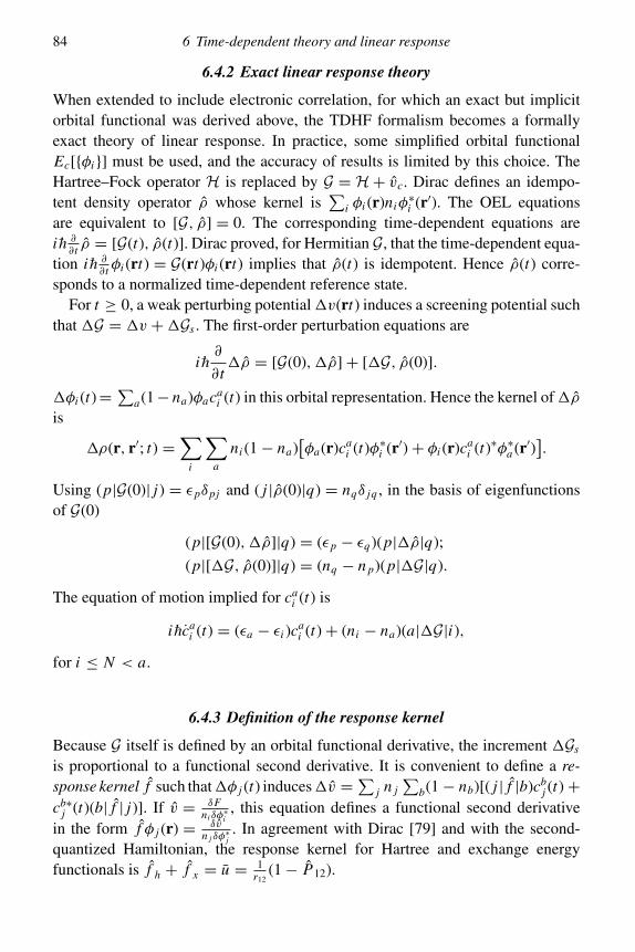
84 6 Time-dependent theory and linear response
6.4.2 Exact linear response theory
When extended to include electronic correlation, for which an exact but implicitorbital functional was derived above, the TDHF formalism becomes a formallyexact theory of linear response. In practice, some simplified orbital functionalEc[{φi }] must be used, and the accuracy of results is limited by this choice. TheHartree–Fock operator H is replaced by G = H+ vc. Dirac defines an idempo-tent density operator ρ whose kernel is
∑i φi (r)niφ
∗i (r′). The OEL equations
are equivalent to [G, ρ] = 0. The corresponding time-dependent equations areih ∂∂t ρ = [G(t), ρ(t)]. Dirac proved, for Hermitian G, that the time-dependent equa-
tion ih ∂∂tφi (rt) = G(rt)φi (rt) implies that ρ(t) is idempotent. Hence ρ(t) corre-
sponds to a normalized time-dependent reference state.For t ≥ 0, a weak perturbing potential�v(rt) induces a screening potential such
that �G = �v +�Gs . The first-order perturbation equations are
ih∂
∂t�ρ = [G(0),�ρ]+ [�G, ρ(0)].
�φi (t)=∑
a(1− na)φacai (t) in this orbital representation. Hence the kernel of�ρ
is
�ρ(r, r′; t) =∑
i
∑a
ni (1− na)[φa(r)ca
i (t)φ∗i (r′)+ φi (r)cai (t)∗φ∗a (r′)
].
Using (p|G(0)| j) = εpδpj and ( j |ρ(0)|q) = nqδ jq , in the basis of eigenfunctionsof G(0)
(p|[G(0),�ρ]|q) = (εp − εq)(p|�ρ|q);
(p|[�G, ρ(0)]|q) = (nq − n p)(p|�G|q).
The equation of motion implied for cai (t) is
ihcai (t) = (εa − εi )c
ai (t)+ (ni − na)(a|�G|i),
for i ≤ N < a.
6.4.3 Definition of the response kernel
Because G itself is defined by an orbital functional derivative, the increment �Gs
is proportional to a functional second derivative. It is convenient to define a re-sponse kernel f such that�φ j (t) induces�v =∑
j n j∑
b(1− nb)[( j | f |b)cbj (t)+
cb∗j (t)(b| f | j)]. If v = δF
ni δφ∗i, this equation defines a functional second derivative
in the form f φ j (r) = δvn j δφ
∗j. In agreement with Dirac [79] and with the second-
quantized Hamiltonian, the response kernel for Hartree and exchange energyfunctionals is f h + f x = u = 1
r12(1− P12).

6.5 Reconciliation of N-electron theory and orbital models 85
The response kernel f c is a linear operator such that f cφ j = δvcn j δφ
∗j. Variations of
unoccupied orbitals δφa (N < a) in the functional Ec are induced by variations ofoccupied orbitals δφi (i ≤ N ) through unitarity. The combined total response kernelis the linear operator f h + f x + f c = f hxc = u + f c.
The equations of motion for the coefficients cai (t) are
ihcai (t) = (εa − εi )c
ai (t)+ (ni − na)
[(a|�v(t)|i)
+∑
j
∑b
{(aj | f hxc|ib)cb
j (t)+ (ab| f hxc|i j)cbj (t)
∗}],for indices i, j ≤ N < a, b. Setting �v(rt) = 2�w(r)�(e−iωt ) for complex fre-quency ω, the independent coefficients defined by
cai (t) = Xa
i e−iωt + Y a∗i eiω∗t
satisfy linear inhomogeneous equations
(εa − εi − hω)Xai + (ni − na)
∑j
∑b
[(aj | f hxc|ib)Xb
j + (ab| f hxc|i j)Y bj
]= −(ni − na)(a|�w|i),
(εa − εi + hω)Y ai + (ni − na)
∑j
∑b
[(i j | f hxc|ab)Xb
j + (ib| f hxc|aj)Y bj
]= −(ni − na)(i |�w|a).
In the exchange-only limit, these are the TDHF or RPA equations (Thouless [407],p. 89). If �w = 0, excitation energies are values of hω for which the determinantof the residual homogeneous equations vanishes.
6.5 Reconciliation of N-electron theory and orbital models
The action integral defined in standard N-electron theory is
AN [!] =∫ t1
t0
dt
⟨ih∂
∂t− H
⟩=∫ t1
t0
dt
{⟨ih∂
∂t
⟩− E[!]
},
where the notation 〈· · ·〉 denotes (!| · · · |!)/(!|!) for an arbitrarily normalizedN-electron wave function !(t). The theory postulates that this action integral isstationary subject to fixed normalization. For comparison, the action integral oforbital functional theory is
A["] =∫ t1
t0
dt
{("
∣∣∣∣ih∂
∂t
∣∣∣∣")− E["]
}.

86 6 Time-dependent theory and linear response
While E["] = E[!], the mean values of the time derivative are not equal. Even ifH is independent of time, these values are constants
∑i niεi and E , respectively.
These constants can be reconciled by inserting a gauge potential γ = E −∑i niεi
into A, determined by equating the time-dependent phase factors. This also pre-serves the normalization ("|!) = ("|") = 1 for the time-dependent wave func-tions, so that the definition of correlation energy Ec = ("|H |! −") remains un-changed. When the Hamiltonian is time-dependent, γ (t) must be determined sothat ("γ |ih ∂
∂t |"γ ) = 〈ih ∂∂t 〉, where "γ incorporates the gauge-dependent phase
factor. For any rule! → " applied for all t0 ≤ t ≤ t1, the time derivative terms inthe action integrals are #s =
∫ t1t0
dt("|ih ∂∂t |") and # = ∫ t1
t0dt〈ih ∂
∂t 〉. The presentargument indicates that a gauge transformation can be introduced such that#s −#drops out of the variational formalism. This is invoked below to remove such a termfrom the equations of time-dependent density functional theory.
6.6 Time-dependent density functional theory (TDFT)
An extension of density functional theory to time-dependent external potentials hasrecently been derived [351, 155]. Hohenberg and Kohn [173] proved, for nondegen-erate ground states, that the electronic density function ρ(r) and the external poten-tial function v(r) mutually determine each other. Easily extended to spin-indexeddensity and potential, this implies that all properties of an N-electron ground stateare functionals of the density function. A slightly more restrictive proof, requiringthe existence of a Taylor expansion of the potential function in time, establishes ananalogous 1–1 correspondence between the (spin-indexed) time-dependent densityfunction ρ(xt) and an external potential v(xt) [351, 155]. This shows that all prop-erties of the time-dependent state that evolves from a given initial state!(t0) in thetime interval t0 ≤ t ≤ t1 are functionals of ρ(xt). This theorem is used to justifya time-dependent density functional theory (TDFT), based on a time-dependentgeneralization of the Kohn–Sham equations. These are modified time-dependentSchrodinger equations
ih∂
∂tφi (xt) = {t + w(xt)}φi (xt),
for each of N occupied orbital functions of a time-dependent model state ", itselfa single Slater determinant. If a Frechet functional derivative [26] of a densityfunctional analogous to E − T exists in this time-dependent theory, it defines aneffective local potentialw(xt) in the orbital equations. If the assumed local effectivepotential is replaced by a more general linear operator or nonlocal potential, thisformalism becomes identical to TOFT, as derived above, which reduces, for anexchange-only model, to the TDHF theory of Dirac [79].

6.6 Time-dependent density functional theory (TDFT) 87
Generalized Hohenberg–Kohn theorems are proved by developing the actionintegrals appropriate to the time-dependent theory [351, 155]. Assumptions canbe minimized by carrying out a time-dependent version of the constrained-searchconstruction of Levy [222, 201]. The variational condition that a certain actionintegral should be stationary subject to the constraint of specified density ρ(xt)is implemented here by introducing the time-dependent external potential v(xt)as a Lagrange-multiplier field for the density constraint. If these equations havea stationary solution, this establishes the property of “v-representability” of thespecified density. An action integral is defined for arbitrarily normalized time-dependent N-electron trial functions !(t) by
B[!(t)] =∫ t1
t0
dt
⟨ih∂
∂t− T − U
⟩.
The N-electron Hamiltonian is H = T + U + V , where the three terms representkinetic energy, interelectronic Coulomb interaction, and an external field, respec-tively. The variational condition that determines  for t0 ≤ t ≤ t1 is
δ
(B[!(t)]−
∫ t1
t0
dt∫
d3x v(xt)[ρ!(xt)− ρ(xt)]
)= 0,
for variations of!within the N-electron Hilbert space. Given a particular fieldv(xt),the stationary condition determines!v(t) through the time-dependent Schrodingerequations, but in general the density ρv(xt) computed from this wave function dif-fers from the specifiedρ(xt). A Lagrange-multiplier field vρ(xt) is to be chosen suchthat ρv(xt) = ρ(xt). Since
∫vρ = ∫ t1
t0dt∫
d3x v(xt)ρ(xt) is constant for given v,Av[ρ] = B[ρ]+ ∫ vρ is defined as a functional of ρ, where B[ρ] = B[!v], eval-uated for v = vρ . This construction must succeed whenever the time-dependentSchrodinger equation has a solution in the interval t0 ≤ t ≤ t1 with !(t0) = !0,and if the Lagrange multiplier field vρ(xt) exists. This latter condition is “v-representability”. These conditions seem very plausible for variations about well-defined physical solutions, but there is no rigorous theory giving general uniquenessand existence conditions. When this construction succeeds, it determines a func-tional Av[ρ] that has a stationary value when ρ(xt) is determined by a solution ofthe time-dependent Schrodinger equation defined by the external potential functionvρ(xt). Uniqueness follows from uniqueness of the solution of this time-dependentequation [351], within a class of equivalent solutions corresponding to gauge trans-formations. The trial functional B is “universal” in the sense that it depends onlyon H − V , the same for all external potentials. However, the variational conditionimplies different results for different initial conditions, !(t0) = !0.
Defining the functional # = ∫ t1t0
dt〈ih ∂∂t 〉, then Av = #−�, where � =∫ t1
t0dt Ev(t). Using Ev(t) = 〈H〉 = 〈 f + V 〉 = F + V , stationary Av implies

88 6 Time-dependent theory and linear response
Euler–Lagrange equations of the form
δ#
δρ= δF
δρ+ v(xt),
if the indicated density functional derivatives exist as Frechet derivatives, equal tomultiplicative local potential functions.
Applying the same argument to a noninteracting N-electron system with the samedensity defines an action integral
Bs["(t)] =∫ t1
t0
dt
("
∣∣∣∣ih∂
∂t− T
∣∣∣∣"),
where the N-electron trial functions are model functions ", in the form of singleSlater determinants. A Lagrange-multiplier fieldwρ(xt) is determined such that thesolution of the variational condition
δ
(Bs["(t)]−
∫ t1
t0
dt∫
d3xw(xt)[ρ"(xt)− ρ(xt)]
)= 0,
determines a density equal to the specified ρ(xt) when w(xt) = wρ(xt). “Nonin-teracting v-representability” is established by any solution of these equations. Thisdefines a “universal” density functional Bs[ρ] when evaluated for ρ and wρ . Forfixed w(xt) but variable ρ, the functional Asw[ρ] = Bs[ρ]+ ∫ wρ is stationarywhen ρ = ρw, the density obtained by solving the noninteracting time-dependentSchrodinger equation in which the time-dependent potential is wρ = w.
Defining the functional #s =∫ t1
t0dt("|ih ∂
∂t |"), then Asw = #s −�s , where
�s =∫ t1
t0dt("|T + W |"). Stationary Asw implies Euler–Lagrange equations of
the form
δ#s
δρ= δTs
δρ+ w(xt),
if the indicated density functional derivatives exist as Frechet derivatives.In the noninteracting problem both required functional derivatives can be eval-
uated from explicit orbital functional derivatives. In detail, δ#sni δφ
∗i= ih ∂
∂tφi andδTs
ni δφ∗i= tφi . For variations of the partial densities ρi = φ∗i φi , this implies Gateaux
functional derivatives [26, 102] δ#sni δρiφi = ih ∂
∂tφi and δTsni δρiφi = tφi . The implied or-
bital Euler–Lagrange equations are the time-dependent Schrodinger equations forthe occupied orbitals i ≤ N ,
ih∂
∂tφi (xt) = (t + w(xt))φi (xt).
Thus for noninteracting electrons, density functional analysis reproduces the usualSchrodinger equations, but a theory based solely on densities (a time-dependent

6.7 Excitation energies and energy gaps 89
Thomas–Fermi theory) requires a Frechet derivative for the kinetic energy, andcannot exist for more than two electrons [288].
For interacting electrons, the required functional derivatives cannot be evaluatedexplicitly. In the TDFT derivation [155], the density functional derivative of thekinetic energy term in� is treated correctly as equivalent to the Schrodinger operatort . Nonetheless, the functional derivative of the exchange-correlation functional isassumed without proof to be a Frechet derivative, equal to a time-dependent localpotential function vxc(xt). It is argued above that the difference functional#−#s
can consistently be set to zero by a gauge transformation. Taking this into account,and assuming that vxc exists, both interacting and noninteracting equations havethe same form, and by construction produce the same density function ρ(xt). Itcan then by inferred that the local potentials in these equations are equal, up to agauge potential γ (t). Then the Kohn–Sham potential could be decomposed intow(xt) = v(xt)+ vh(xt)+ vxc(xt). Hence if a Frechet derivative vxc did exist, thecorrect interacting ρ(xt) would be obtained by solving the implied time-dependentKohn–Sham equation.
This proposition has been tested in the exact-exchange limit of the impliedlinear-response theory [329]. The TDFT exchange response kernel disagrees qual-itatively with the corresponding expression in Dirac’s TDHF theory [79, 289]. Thiscan be taken as evidence that an exact local exchange potential does not existin the form of a Frechet derivative of the exchange energy functional in TDFTtheory.
6.7 Excitation energies and energy gaps
Time-dependent OFT implies matrix equations for excitation energies hω,
(εa − εi − hω)Xai + (ni − na)
∑j
∑b
[(aj | f hxc|ib)Xb
j + (ab| f hxc|i j)Y bj
] = 0,
(εa − εi + hω)Y ai + (ni − na)
∑j
∑b
[(i j | f hxc|ab)Xb
j + (ib| f hxc|aj)Y bj
] = 0.
The simplest internally consistent approximation to an excitation energy is ob-tained by limiting the summation to the diagonal term j, b = i, a. The second linevanishes because of antisymmetry, (i i | f hxc|aa) ≡ 0, and the first line reduces to asingle equation,
{εa − εi − hω − (ai | f hxc|ai)}Xai = 0.
Neglecting correlation response, this implies a well-known formula for zeroeth-order hole–particle excitation energies [261, 149], hω = εa − εi − (ai |u|ai). Thetwo-electron integral here depends strongly on orbital localization. Since the lower

90 6 Time-dependent theory and linear response
state is stationary, this energy difference should be minimized to represent astationary excited state. This can be done by separate localization transformationsof occupied and unoccupied orbitals. This provides a mechanism to reduce Hartree–Fock band gaps, which are systematically too large. The correlation response kernelhas the physical effect of screening the interelectronic Hartree and exchange terms.This implies direct effects on energy gaps, evident in the TOFT formalism.
III
Continuum states and scattering theory
This part extends quantum variational theory to continuum states. In par-ticular, variational principles are developed for wave function continu-ity at specified energy, which is the usual context of scattering theory.Chapter 7, concerned with multiple scattering theory, lies somewhere be-tween the theory of bound states and true scattering theory. Formalismappropriate to the latter is adapted to computing the electronic structure oflarge molecules and periodic solids, whose energy levels are determinedby consistency conditions for wave function continuity. A variationalformalism is derived for energy linearization. Chapter 8 develops vari-ational principles and methods suitable for the true continuum problemof electron scattering at specified energy. Chapter 9 presents method-ology, some very recent, that allows rotational and vibrational effects inelectron–molecule scattering to be treated as a practicable extension offixed-nuclei variational theory.


7
Multiple scattering theory for molecules and solids
The principal references for this chapter are:
[52] Butler, W.H. and Zhang, X.-G. (1991). Accuracy and convergence properties ofmultiple-scattering theory in three dimensions, Phys. Rev. B 44, 969–983.
[113] Ferreira, L.G. and Leite, J.R. (1978). General formulation of the variational cellularmethod for molecules and crystals, Phys. Rev. A 18, 335–343.
[148] Gonis, A. and Butler, W.H. (2000). Multiple Scattering in Solids (Springer, NewYork).
[203] Kohn, W. (1952). Variational methods for periodic lattices, Phys. Rev. 87, 472–481.[204] Kohn, W. and Rostoker, N. (1954). Solution of the Schrodinger equation in periodic
lattices with an application to metallic lithium, Phys. Rev. 94, 1111–1120.[277] Nesbet, R.K. (1990). Full-potential multiple scattering theory, Phys. Rev. B 41,
4948–4952.[279] Nesbet, R.K. (1992). Variational principles for full-potential multiple scattering
theory, Mat. Res. Symp. Proc. 253, 153–158.[359] Schlosser, H. and Marcus, P. (1963). Composite wave variational method for
solution of the energy-band problem in solids, Phys. Rev. 131, 2529–2546.[384] Skriver, H.L. (1984). The LMTO Method (Springer-Verlag, Berlin).[432] Williams, A.R. and Morgan, J. van W. (1974). Multiple scattering by non-muffin-tin
potentials: general formulation, J. Phys. C 7, 37–60.
For direct N-electron variational methods, the computational effort increases sorapidly with increasing N that alternative simplified methods must be used forcalculations of the electronic structure of large molecules and solids. Especiallyfor calculations of the electronic energy levels of solids (energy-band structure),the methodology of choice is that of independent-electron models, usually in theframework of density functional theory [189, 321, 90]. When restricted to localpotentials, as in the local-density approximation (LDA), this is a valid variationaltheory for any N-electron system. It can readily be applied to heavy atoms byrelativistic or semirelativistic modification of the kinetic energy operator in theorbital Kohn–Sham equations [229, 384].
93

94 7 Multiple scattering theory for molecules and solids
Solution of the one-electron Schrodinger or modified Dirac equation for a systemof many atoms is still a difficult computational task. This has been simplified andmade tractable by the methodology of multiple scattering theory (MST), recentlyreviewed by Gonis and Butler [148]. These authors concentrate on methods in whichorbital energy levels are identified by searching for roots of a secular determinantappropriate to the Kohn–Sham equations. Although MST uses the formalism ofscattering theory, it is used in practice as a bound-state method, computing en-ergy levels by varying a specified energy until continuity conditions are satisfied.In particular, the electronic energy bands of regular periodic solids for specifiedtranslational quantum numbers (momentum vectors in a reduced Brillouin zone[384, 148]) are defined as a discrete set of energy values that cause a secular deter-minant to vanish. True continuum scattering theory is discussed in the followingchapter.
At the cost of introducing an additional level of approximation, root-searchmethodology can be replaced within some fixed interval of electronic energy lev-els (an energy panel or window) by an energy-linearized method which requiressolution of a matrix eigenvalue problem for energy eigenvalues within the panel.Because of the very substantial relative gain in efficiency, such linearized methods[384] are by far the most widely used in energy-band calculations. Both root-searchand energy-linearized MST methods require iteration to self-consistency, converg-ing when the computed density function is sufficiently close to that used to constructthe potential function in the current iteration. This requires accurate solution of thePoisson equation determined by the input density function, which is also simplifiedby an adaptation of MST [148].
In addition to the model approximation implied by a restriction to local exchangeand correlation potentials, the methodology has often been further simplified by themuffin-tin model. In this model, each atom of a molecule or solid is surrounded bya muffin-tin sphere, of sufficiently small radius that adjacent spheres do not over-lap. The local potential function is spherically averaged within each such sphere,and set to a constant value (the muffin-tin zero) in the interstitial volume betweenthese spheres. This mathematical model greatly simplifies the required computa-tional effort. It is physically justifiable for metals, since the interstitial region isdescribed in terms of electronic free wave functions, but it is counterintuitive foratoms in molecules, since electronic exchange and correlation in chemical bondsmust be treated accurately. Earlier work restricted to the muffin-tin model has beensupplanted by full-potential methodology in recent years, based on the full localpotential of the Kohn–Sham model, without simplifying approximations.
The most natural geometrical framework for full-potential methodology is thatof space-filling polyhedral atomic cells, mathematically a Voronoi lattice construc-tion in three dimensions. Space is subdivided by perpendicular bisector planes of

7.1 Full-potential multiple scattering theory 95
the internuclear coordinate vectors. This lattice construction corresponds to theWigner–Seitz [429] cellular model. For open lattice structures (e.g. the diamondlattice), it is common practice to introduce empty cells, with no enclosed atomic nu-cleus, to provide a more uniform space-filling structure. Variational principles andmethods appropriate to such space-filling cellular lattices will be discussed here.The muffin-tin model is a simplified special case in this general theory. A closelyrelated approximation, the atomic sphere model [384], extends the spherically aver-aged local potential of the muffin-tin sphere throughout a concentric sphere whosevolume equals that of the Wigner–Seitz polyhedral atomic cell. This can be ex-tended to the full enclosing sphere of each polyhedral atomic cell, which greatlysimplifies the computation of atomic basis functions required in full-potential MST.These spherically averaged potentials can be considered as initial approximationsto be used during self-consistency iterations, to be modified following convergenceby nonspherical potential terms to be treated as perturbations in the context of linearresponse theory. Nonlocal corrections to an initial local-potential model may alsobe included in principle within such a linear-response theory.
7.1 Full-potential multiple scattering theory
Since the principal applications of MST are in solid-state theory, which traditionallyuses Rydberg rather than Hartree units of energy, this convention will be followedin the present chapter. Restricting the formalism to local potential functions as inKohn–Sham theory, the Schrodinger equation for an electron of positive energy is
(∇2 + κ2)ψ(x) = v(x)ψ(x),
where the one-electron energy is defined by ε = κ2 (Ryd). The momentum κ isa parameter that characterizes electronic energies above a zero value assigned tothe lowest energy of an energy band. Since this Schrodinger equation is formallya modified Helmholtz equation, it is convenient to introduce a Helmholtz Greenfunction defined such that
(∇2 + κ2)G0(x, x′) = δ(x, x′).The Green function must satisfy boundary conditions at large distances consis-tent with the wave function ψ . The Schrodinger equation can be replaced by anequivalent Lippmann–Schwinger integral equation
ψ(x) = χ (x)+∫�3
G0(x, x′)v(x′)ψ(x′) d3x′,
where χ is a solution of the homogeneous Helmholtz equation. In an operatornotation this is ψ = χ + G0vψ . For a solid or molecule, coordinate space �3 can
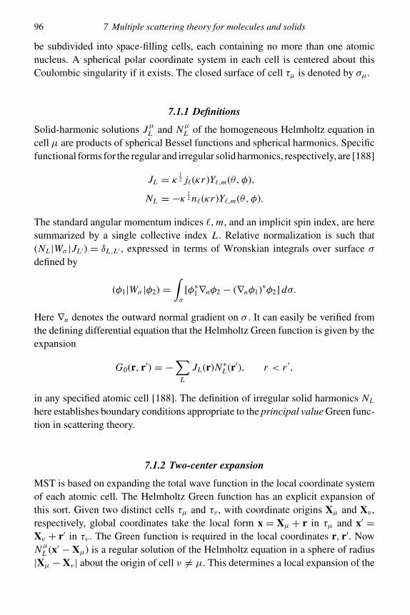
96 7 Multiple scattering theory for molecules and solids
be subdivided into space-filling cells, each containing no more than one atomicnucleus. A spherical polar coordinate system in each cell is centered about thisCoulombic singularity if it exists. The closed surface of cell τµ is denoted by σµ.
7.1.1 Definitions
Solid-harmonic solutions JµL and NµL of the homogeneous Helmholtz equation incell µ are products of spherical Bessel functions and spherical harmonics. Specificfunctional forms for the regular and irregular solid harmonics, respectively, are [188]
JL = κ 12 j�(κr )Y�,m(θ, φ),
NL = −κ 12 n�(κr )Y�,m(θ, φ).
The standard angular momentum indices �,m, and an implicit spin index, are heresummarized by a single collective index L . Relative normalization is such that(NL |Wσ |JL ′) = δL ,L ′ , expressed in terms of Wronskian integrals over surface σdefined by
(φ1|Wσ |φ2) =∫σ
[φ∗1∇nφ2 − (∇nφ1)∗φ2] dσ.
Here ∇n denotes the outward normal gradient on σ . It can easily be verified fromthe defining differential equation that the Helmholtz Green function is given by theexpansion
G0(r, r′) = −∑
L
JL (r)N ∗L (r′), r < r ′,
in any specified atomic cell [188]. The definition of irregular solid harmonics NL
here establishes boundary conditions appropriate to the principal value Green func-tion in scattering theory.
7.1.2 Two-center expansion
MST is based on expanding the total wave function in the local coordinate systemof each atomic cell. The Helmholtz Green function has an explicit expansion ofthis sort. Given two distinct cells τµ and τν , with coordinate origins Xµ and Xν ,respectively, global coordinates take the local form x = Xµ + r in τµ and x′ =Xν + r′ in τν . The Green function is required in the local coordinates r, r′. NowNµL (x′ − Xµ) is a regular solution of the Helmholtz equation in a sphere of radius|Xµ − Xν | about the origin of cell ν �= µ. This determines a local expansion of the

7.1 Full-potential multiple scattering theory 97
form
NµL (r′ + Xν − Xµ) = −∑
L ′J νL ′(r
′)gνµL ′,L ,
for r ′ < |Xµ − Xν |. On substituting this into the one-center expansion,
G0(Xµ + r,Xν + r′) =∑
L
∑L ′
JµL (r)gµνL ,L ′ Jν∗L ′ (r′),
for r, r ′ < |Xµ − Xν |. The Hermitian matrix gµνL ,L ′ defines structure constants forthe two-center expansion of the Green function in locally regular solid harmonics.Through the Lippmann–Schwinger equation, matrix g propagates a given wavefunction in one cell into incremental wave functions in the other cell. MST collectsthe total incremental wave function in each cell as a multicenter expansion, toestablish a linear consistency condition for a molecule or solid. For a regular periodiclattice, contributions from outside an elementary polyatomic translational cell aremultiplied by translational phase factors and summed over an infinite space-lattice.
7.1.3 Angular momentum representation
An eigenfunctionψ of the Schrodinger equation satisfies the homogeneous integralequation ψ = ∫
�3 G0vψ . In cell τ this defines a locally regular solution of theHelmholtz equation
χ = ψ −∫τ
G0vψ =∫�3−τ
G0vψ,
consistent with the Lippmann–Schwinger equation.The function χ can be represented in τ by a sum of regular solid harmonic
functions,
χ (r) =∑
L
JL (r)CL .
Similarly, because ψ is regular at the local coordinate origin, it can be representedat this origin by
ψ(r) =∑
L
JL (r)cL .
From the Lippmann–Schwinger equation and the expansion of G0 in some spec-ified cell τµ, the coefficients in these expansions must be related by CµL =cµL +
∫τµ
N ∗Lvψ . Consistency conditions are derived by considering the alternative
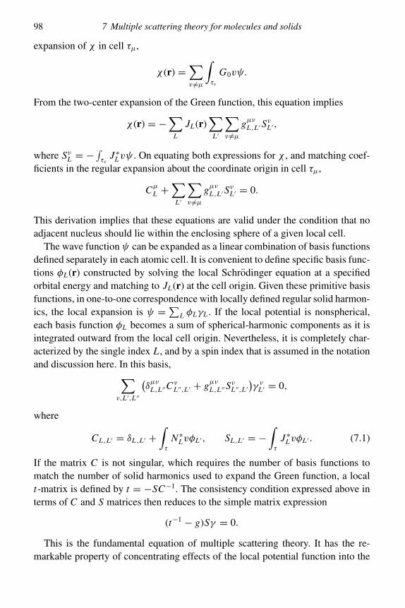
98 7 Multiple scattering theory for molecules and solids
expansion of χ in cell τµ,
χ (r) =∑ν �=µ
∫τν
G0vψ.
From the two-center expansion of the Green function, this equation implies
χ (r) = −∑
L
JL (r)∑
L ′
∑ν �=µ
gµνL ,L ′SνL ′,
where SνL = −∫τν
J ∗Lvψ . On equating both expressions for χ , and matching coef-ficients in the regular expansion about the coordinate origin in cell τµ,
CµL +∑
L ′
∑ν �=µ
gµνL ,L ′SνL ′ = 0.
This derivation implies that these equations are valid under the condition that noadjacent nucleus should lie within the enclosing sphere of a given local cell.
The wave functionψ can be expanded as a linear combination of basis functionsdefined separately in each atomic cell. It is convenient to define specific basis func-tions φL (r) constructed by solving the local Schrodinger equation at a specifiedorbital energy and matching to JL (r) at the cell origin. Given these primitive basisfunctions, in one-to-one correspondence with locally defined regular solid harmon-ics, the local expansion is ψ =∑
L φLγL . If the local potential is nonspherical,each basis function φL becomes a sum of spherical-harmonic components as it isintegrated outward from the local cell origin. Nevertheless, it is completely char-acterized by the single index L , and by a spin index that is assumed in the notationand discussion here. In this basis,∑
ν,L ′,L ′′
(δµν
L ,L ′′CνL ′′,L ′ + gµνL ,L ′′S
νL ′′,L ′
)γ νL ′ = 0,
where
CL ,L ′ = δL ,L ′ +∫τ
N ∗LvφL ′, SL ,L ′ = −
∫τ
J ∗LvφL ′ . (7.1)
If the matrix C is not singular, which requires the number of basis functions tomatch the number of solid harmonics used to expand the Green function, a localt-matrix is defined by t = −SC−1. The consistency condition expressed above interms of C and S matrices then reduces to the simple matrix expression
(t−1 − g)Sγ = 0.
This is the fundamental equation of multiple scattering theory. It has the re-markable property of concentrating effects of the local potential function into the

7.1 Full-potential multiple scattering theory 99
t-matrix, separately determined in each local atomic cell, while the geometry ofthe polyatomic superstructure is entirely characterized by the matrix g of structureconstants. For a regular periodic solid, the matrices here are summed over equiv-alent translational cells, with coefficient phase factors that depend on an effectivemomentum vector k, to give
{t−1(ε)− g(ε; k)}S(ε)γ (ε; k) = 0.
The Korringa–Kohn–Rostoker (KKR) method [207, 204] is implemented by search-ing for the zeroes of the secular determinant det(t−1 − g), or det(I − tg) if t issingular.
The single-site matrix t corresponds to a scattering operator t defined bytχL = vφL for any primitive basis orbital φL in a given atomic cell. HereχL = φL −
∫τ
G0vφL =∑
L ′ JL ′CL ′,L . From this definition it follows that t JL =v∑
L ′ φL ′(C−1)L ′,L . The t-matrix is
(JL |t |JL ′) =∑L ′′
(JL |v|φL ′′)(C−1)L ′′,L ′ .
This implies that t = −SC−1, since (JL |v|φL ′) = −SL ,L ′ .
7.1.4 The surface matching theorem
Consider an atomic cell τ with closed boundary surfaceσ . Given a functionψ and itsnormal gradient∇nψ on the surface σ , a unique solution of the Helmholtz equationis determined by either inward or outward integration. Because this global functionis completely determined on σ , it in general will be singular at the coordinateorigin of cell τ and unbounded at infinite distance from this center. Inward integra-tion in general gives a singular function, which includes irregular functions N .For a function that is regular at the origin, either ψ (classical Dirichlet problem),or ∇nψ (Neumann problem) can be specified on σ , but not both [74, 255]. Anexpansion valid on surface σ will be established here, determined by both the valueand normal gradient of ψ . Consistency of the surface Wronskian integrals impliesthat coefficients of an expansion in both JL and NL must be given by
ψ(rσ )≡σ∑
L
[JL (NL |Wσ |ψ)− NL (JL |Wσ |ψ)]
if the sums converge. The notation here denotes matching of both function valueand normal gradient. Even if the separate series in functions JL and NL do notconverge, it can be shown that well-defined functions exist, providing summationformulas for the possibly divergent series. This justifies formal operations in MSTthat depend on Wronskian integrals of this expansion.

100 7 Multiple scattering theory for molecules and solids
An interior function χ (r) = −(G0(r, rσ )|Wσ |ψ) is defined that is regular at thecell origin. The one-center expansion of the Green function converges in the largestsphere enclosed by surface σ , sphere S0 of radius r0. This determines a series ex-pansion χ (r) =∑
L JL (NL |Wσ |ψ), valid for r < r0. Similarly, an exterior func-tion η(r) = (G0(r, rσ )|Wσ |ψ) is defined that is bounded at infinite separation.Again using the convergent expansion of the Green function, but in the exteriorregion outside an enclosing sphere S1 of radius r1, η(r) = −∑L NL (JL |Wσ |ψ)for r > r1.
The auxiliary functions χ and η have finite values on σ because the surface areaelement removes the singularity of the Green function in their defining surface inte-grals. Both functions are defined throughout the region r0 ≤ r ≤ r1. The boundaryconditions determine unique solutions of the Helmholtz equation for integration ofχ outward from S0 and of η inward from S1. Similarly, the function ψ given on σcan be extended throughout this region by integrating the Helmholtz equation bothinwards to S0 and outwards to S1. Green’s theorem implies for such solutions ofthe Helmholtz equation that Wronskian surface integrals are conserved on nestedclosed surfaces. Hence the difference functionψ − χ − η has vanishing Wronskianintegrals with all regular and irregular solid harmonics on both spherical surfacesS0 and S1. It follows from Green’s theorem that this difference function must vanishidentically in the region between these two surfaces, and in particular on surface σ .This establishes the surface matching theorem [280],
limr→rσ−
χ + limr→rσ+
η≡σ ψ(rσ ).
The series expansion ofχ may diverge in the interior moon region [148], betweenthe enclosed sphere S0 and σ , while the corresponding series for η may divergebetween σ and S1. Nonetheless, these functions are well defined by Wronskianintegrals of the Green function, independently of such expansions. The impliedsurface integrals are properties of the integrated functions, and justify formal useof the surface series expansion in boundary matching conditions based on theseWronskian integrals. If applied to basis functions that are solutions of the sameSchrodinger equation in τ , for which (φi |Wσ |φ j ) = 0, surface expansion of eitherfunction implies∑
L
(φi |Wσ |JL )(NL |Wσ |φ j )−∑
L
(φi |Wσ |NL )(JL |Wσ |φ j ) = 0.
7.1.5 Surface integral formalism
Formalism from scattering theory, to be developed in a later chapter, shows thata function ψ and its normal gradient on a closed surface σ can be matched to a

7.1 Full-potential multiple scattering theory 101
linear combination of regular internal solutions of a Schrodinger equation if andonly if
ψ(rσ ) =∫σ
�(ε; rσ , r′σ )∇nψ(r′σ ) dr′σ .
Here � is an Hermitian linear integral operator over σ that can be constructedvariationally from basis solutions {φi } of the Schrodinger equation that are regularin the enclosed volume. The functions φi do not have to be defined outside theenclosing surface and in fact must not be constrained by a fixed boundary condi-tion on this surface [270]. This is equivalent to the Wronskian integral condition(φi |Wσ |ψ) = 0, for all such φi . When applied to particular solutions of the formψ = J − Nt on σ ,
(φi |Wσ |JL )−∑
L ′(φi |Wσ |NL ′)tL ′,L = 0.
This equation determines the local t-matrix. Any local basis function φi has theformal expansion on σ
φi ≡σ∑
L
[JL (NL |Wσ |φi )− NL (JL |Wσ |φi )].
Canonical basis orbitals are defined here such that φL → JL at the local cell origin.Introducing a matrix notation for surface Wronskian integrals,
CL ,L ′ = (NL |Wσ |φL ′), SL ,L ′ = −(JL |Wσ |φL ′), (7.2)
the formal expansion of a primitive basis orbital φL on σ is
φL ≡σ∑
L ′(JL ′CL ′,L + NL ′SL ′,L ).
The surface Wronskian integrals C and S defined here are identical with the volumeintegrals defined in Eqs. (7.1). Using (∇2 + κ2)φL = vφL , integration by parts ofthe MST volume integrals, Eqs. (7.1), gives equivalent surface integrals, verifyingEqs. (7.2),
SL ,L ′ = −∫τ
J ∗L (∇2 + κ2)φL ′ = −(JL |Wσ |φL ′),
CL ,L ′ = δL ,L ′ +∫τ
N ∗L (∇2 + κ2)φL ′ = (NL |Wσ |φL ′).
7.1.6 Muffin-tin orbitals and atomic-cell orbitals
Deriving an energy-linearized version of MST, Andersen [12, 9] introduced muffin-tin orbital (MTO) basis functions. These functions have the form φ − χ inside S0,

102 7 Multiple scattering theory for molecules and solids
the enclosed sphere of an atomic cell, and η outside. Here φ is a local solution ofthe Schrodinger equation, while χ and η are sums of regular and irregular solidharmonics, respectively. The matching on S0 is exact in the muffin-tin model,so that these functions provide a basis set suitable for variational calculations.In practice, because the long-range η functions are not orthogonal to inner shellfunctions in displaced atoms [193], they are expanded in the energy derivatives φ ofthe basis functions φ. The resulting linearized muffin-tin orbital (LMTO) method[13, 9, 384] solves the Schrodinger secular equation in an MTO basis, constructedusing KKR/MST structure constants.
The surface matching theorem makes it possible to generalize the idea of muffin-tin orbitals to a nonspherical Wigner–Seitz cell τ . Each local basis orbital is rep-resented as φ≡σ χ + η on the cell surface σ , where χ and η are the auxiliaryfunctions defined by the surface matching theorem. An atomic-cell orbital (ACO)is defined as the function φ − χ , regular inside τ . By construction, the smoothcontinuation of this ACO outside τ is the function η. The specific functionalforms are
χL =∑
L ′JL ′CL ′,L , ηL =
∑L ′
NL ′SL ′,L .
Either MTO or ACO functions are valid as basis functions for expanding a globalwave function ψ in all atomic cells. By construction, they are regular in τ , smoothat σ , and bounded outside. When the matrix C is nonsingular, modified canonicalbasis functions can be defined such that
φL =∑
L ′φL ′(C
−1)L ′,L ,
so that the auxiliary regular function is χL = JL . The corresponding ACO functiontakes the especially simple form φL − JL , matched on the cell surface σ to ηL =−∑L ′ NL ′ tL ′,L .
7.1.7 Tail cancellation and the global matching function
As discussed by Andersen [9, 10] for muffin-tin orbitals, the locally regular com-ponents χ defined in each muffin-tin sphere are cancelled exactly if expansioncoefficients satisfy the MST equations (the tail-cancellation condition) [9, 384].The standard MST equations for space-filling cells can be derived by shrinking theinterstitial volume to a honeycomb lattice surface that forms a common boundaryfor all cells. The wave function and its normal gradient evaluated on this honeycombinterface define a global matching function ξ (σ ).

7.1 Full-potential multiple scattering theory 103
In any cell τ = τµ, with surface σ = σµ, any solution ψ of the Lippmann–Schwinger equation defines auxiliary functions χ in = ψ − ∫
τG0vψ and χout =∫
�3−τ G0vψ , which are equal by construction. After integration by parts,
χ in = −(G0|Wµ|ψ) =∑
L
JµL(N µ
L |Wµ|ψ).
The notation Wµ defines a Wronskian integral over σµ. By the surface match-ing theorem, χ in = χ , the interior component of ψ . Since ψ is a solution of theLippmann–Schwinger equation, this implies χout = χ in when evaluated in the inte-rior of τµ. This is a particular statement of the tail-cancellation condition. To showthis in detail, after integration by parts
χout =∑ν �=µ
(G0|Wν |ψ) =∑ν �=µ
∑L ′,L
JµL ′gµν
L ′,L(J νL |Wν |ψ
),
which determines the standard MST equations.On substituting the expansion N νL = −
∑L ′ JµL ′g
µν
L ′,L ,
χout = −∑ν �=µ
∑L
N νL(J νL |Wν |ψ
).
For comparison, η = −∑L NµL (JµL |Wµ|ψ) is the exterior component of ψ on σ =σµ. Since χout≡σ χ on σ and ξ ≡σ χ + η, this determines ξ everywhere on theglobal matching surface,
ξ ≡σ∑ν
ην =∑ν
∑L
N νLβνL , (7.3)
where βνL = −(J νL |Wν |ψ). If the sum here diverges, specific integrated functionsην should be used.
All Wronskian integrals ofψ − ξ should vanish on the honeycomb lattice. Giventhe local expansion ψ =∑
L φµ
Lγµ
L in any particular cell τµ, (JµL |Wµ|ψ − ξ ) = 0determines βµL =
∑L ′ SµL ,L ′γ
µ
L ′ . (NµL |Wµ|ψ − ξ ) = 0 implies that∑ν,L ′,L ′′
(δµν
L ,L ′′CνL ′′,L ′ + gµνL ,L ′′S
νL ′′,L ′
)γ νL ′ = 0. (7.4)
These are the standard MST equations, in the form (t−1 − g)Sγ = 0, where
t = −SC−1 = (J |Wσ |φ)(N |Wσ |φ)−1. (7.5)
7.1.8 Implementation of the theory
The computational survey of electronic structure of metals by Moruzzi et al. [256] isa landmark example of the original KKR formalism, using the muffin-tin model and

104 7 Multiple scattering theory for molecules and solids
a root-search algorithm. The historical development of MST, from Huygens’ princi-ple and the original formulation by Lord Rayleigh [337, 338] to recent applicationsof full-potential theory, is surveyed by Gonis and Butler [148]. The full-potentialtheory was first proposed by Morgan and Williams [431, 432]. Nonspherical cellboundaries defined by the walls of polyhedral atomic cells were replaced by non-spherical enclosing potentials. This methodology was simplified when it was rec-ognized [39, 40] that viable basis orbitals could be computed within the enclosingsphere S1, and then matched after computation to a variational wave function atthe polyhedral cell boundaries. Ultimately, it was shown that these two apparentlydisparate approaches necessarily produce the same orbital basis functions withinthe enclosed atomic cell [277]. In the surface integral formalism developed here, itis clear that the continuation of basis functions outside a local cell boundary cannotaffect the C and S matrices that characterize MST. This formalism also providesa proof of the validity of MST for nonspherical atomic cells and potentials, whichwas disputed over a decade [148].
7.2 Variational principles
7.2.1 Kohn–Rostoker variational principle
Kohn and Rostoker [204] (KR) derived the KKR method using variational theorywith a functional designed to produce the Lippmann–Schwinger equation. Localbasis solutions can be computed to high accuracy within each unit cell. The vari-ational formalism optimizes the construction of linear combinations of these localsolutions that are compatible with the functions propagated from all adjacent cells.In this version of MST, local solutions are coupled through the free-scatteringGreen function of the Helmholtz equation. The Kohn–Rostoker variational func-tional [204],
� =∫�3ψ∗v
(ψ −
∫�3
G0vψ
)
is stationary for infinitesimal variations of the one-electron wave function ψ ifand only if it satisfies the homogeneous Lippmann–Schwinger equation, ψ =∫�3 G0vψ . The Green function G0 satisfies the inhomogeneous Helmholtz equation
at a specified energy ε = κ2 (Ryd),
(∇2 + κ2)G0(x, x′) = δ(x, x′).The KR variational principle determines a wave function with correct boundaryconditions at a specified energy, the typical conditions of scattering theory. Energyvalues are deduced from consistency conditions.

7.2 Variational principles 105
The KR variational principle and the resulting KKR/MST formalism determinewave functions for bound energy levels of a molecule or of a regular periodicsolid or two-dimensional periodic surface. In these applications, the homogeneousLippmann–Schwinger equation has no valid solutions except at a discrete set ofenergy levels. Hence either κ must be adjusted to meet the conditions for sucha solution, or else the potential function must be altered to v(x)−�ε so thatthe parameter �ε can be varied while retaining the same G0. Using the positiveparameter κ2 to define G0 already implies that energy values are measured relative tothe minimum of an energy band. Because it simplifies functional forms of the Greenfunction and solid harmonics, κ2 = 0 is often used in LMTO calculations [384].
In a true scattering problem, an incident wave is specified, and scattered wavecomponents of ψ are varied. In MST or KKR theory, the fixed term χ in the fullLippmann–Schwinger equation,ψ = χ + ∫ G0ψ , is required to vanish.χ is a solu-tion of the Helmholtz equation. In each local atomic cell τ of a space-filling cellularmodel, any variation of ψ in the orbital Hilbert space induces an infinitesimal vari-ation of the KR functional of the form δ� = ∫
τδψ∗v(ψ − ∫�3 G0vψ)+ hc. This
can be expressed in the form
δ� =∫τ
δψ∗v(χ in − χout)+ hc,
where, integrating the finite volume integrals by parts, and using the coefficientmatrices defined in MST,
χ in = ψ −∫τµ
G0vψ =∑
L
JLCµL ,
χout =∑ν �=µ
∫τν
G0vψ = −∑ν �=µ
∑L ,L ′
JL gµνL ,L ′SνL ′ .
In a finite basis of primitive functions φµL , the stationary condition is
−δ� =∑L ,L ′δ㵆L
∑L1,L2
Sµ†L L1
∑ν
(δµν
L1 L2CνL2 L ′ + gµνL1 L2
SνL2 L ′)γ νL ′ + hc = 0,
which implies the standard MST equations. Energy eigenvalues are determined byadjusting the trial energy so that the secular determinant of the matrix of MSTequations is singular. Continuity conditions at cell boundaries are not addressedby this variational principle. It is usually assumed that ψ lies in the orbital Hilbertspace (continuous function value and normal gradient at any cell interface). Theseconditions are required for consistency with the Schrodinger equation, but are notrequired by the KR variational principle and the MST equations.

106 7 Multiple scattering theory for molecules and solids
7.2.2 Convergence of internal sums
In the Kohn–Rostoker variational equation, the summation indices refer to two dif-ferent classes of functions: orbital basis functionsφL , and solid harmonics JL for thematrix of structure constants. For smooth matching at cell boundaries, the JL sumsshould be carried to completion. In practice, finite sets of basis orbital functions andof solid harmonics are used. The set φL is truncated at some maximum orbital an-gular momentum �φ in each inequivalent atomic cell, and the local expansion of theHelmholtz Green function is limited to some maximum �g. In the muffin-tin model[204], a spherically averaged local potential does not couple different sphericalharmonics in a single cell, but a propagated wave function in general has an infiniteexpansion in other cells because of the Green function. The k-dependent Greenfunction for a periodic lattice structure introduces angular-momentum couplinginto the translational cell even if it is spherical.
Model studies of full-potential KKR theory were carried out for both two-dimensional [51] and three-dimensional [52] space-lattices. The essential conclu-sion is that the truncation parameters �φ and �g influence convergence in differentways, and should not ordinarily be set to a common value �. Adequately convergedresults in general require essentially complete convergence of the geometrical ex-pansion, which determines the Green function in the KR variational principle. Incontrast, high angular momentum values are less significant for the shell structureof an atomic cell, considered to be a distorted atom. This can be understood be-cause high orbital �-values imply a centrifugal potential that excludes any orbitalwave function if the classical turning radius is greater than the enclosing radius ofthe cell. Thus Rydberg orbitals in solids have no direct physical meaning if theRydberg radius extends into the valence shell of adjacent atoms. For these reasons,the C and S matrices should be treated as rectangular column matrices, with therow index �g significantly greater than the column index �φ [52].
Because rectangular matrices are singular, effective closure of these internal sumsover solid-harmonic indices requires a generalized definition of t = −SC−1 andof other expressions that involve inverse matrices in MST [280]. As the index Lincreases, the standard coefficient matrices S and C have very different behavior.The effect of the centrifugal barrier for high orbital �-values is to make the regularsolid harmonics JL very small on any finite cell boundary, while standard normal-ization forces the irregular harmonics to be very large. In this Born-approximationlimit, the low-order matrix C is extended by a unit matrix, while S is extendedby a matrix of zeroes [281]. Thus the matrix t = −SC−1 is augmented by a nullmatrix, while t−1 is augmented by elements of rapidly increasing magnitude, whosecomputational numerical errors can overwhelm the computationally accurate low-order elements. This can account for the strikingly different behavior found in

7.2 Variational principles 107
empty-lattice calculations on the square-planar lattice using the KKR expressiont−1 − g [107] and using the formally equivalent expression I − tg [438]. The lat-ter calculations demonstrated exponential convergence with increasing L indices,while reproducing the much slower and less systematic convergence of the formercalculations when the inverse matrix t−1 was explicitly truncated.
This problem can be avoided by expressing the MST equations in terms ofthe square matrix S†C = C†S, Hermitian in consequence of the surface-matchingtheorem. This matrix has full rank because it is contracted over the larger index �g.From the definitions of the C and S matrices, the matrix product S†C is a specificintegral involving the Helmholtz Green function [281],
∑L ′′
Sµ†L ,L ′′Cµ
L ′′,L ′ = −∫τµ
φµ∗L v
(φµ
L ′ −∫τµ
G0vφµ
L ′
),
which can be evaluated in closed form. The contracted matrix product gS canalso be evaluated in closed form by defining a generalized C-matrix, for displacedirregular solid harmonics N , C
µν
L1,L = (NµL1|Wν |φνL ). The function NµL1
defined incell τµ is evaluated on the surface σν of a displaced cell. This is justified becauseN -functions are valid outside their cell of definition. Using the Green function topropagate Nµ, this becomes C
µν
L1,L =−∑
L2gµνL1 L2
(J νL2|Wν |φνL ) =∑
L2gµνL1 L2
SνL2,L.
In a matrix notation omitting L indices and summations, the KKR/MST equation is
Sµ†∑ν
(δµνCν + gµνSν)γ ν =∑ν
�µνγ ν = 0,
where all matrix products are contracted over the long dimension. In the Hermitianmatrix � the triple product Sµ†gµνSν = Sµ†Cµν = (C
†)µνSν . Multiplying on the
left by S(S†C)−1, and using (C†)µν = Sµ†gµν , this takes the form�β = 0, defining
a modified secular matrix
�µν = δµν + Sµ(Sµ†Cµ)−1(C†)µν.
The coefficients β = Sγ are the expansion coefficients of the global matchingfunction ξ (σ ) =∑
µ,L NµL (rσ )βµL . Defining t = −S(S†C)−1S†, which reduces tot = −SC−1 for square matrices [281], �µν takes the standard MST form I − tg,without implying inversion of a rectangular matrix. Using these closed forms, thecoefficients β and γ are related by
γ µ = −(Sµ†Cµ)−1∑ν �=µ
(C†)µνβν.
In alloy theory, this equation determines the variational wave function for an atomiccell τµ embedded in a statistical medium defined by the vector of coefficients β forall other cells [157, 281].

108 7 Multiple scattering theory for molecules and solids
7.2.3 Schlosser–Marcus variational principle
Since a large truncation parameter �g implies large unsymmetrical C and S ma-trices, and a very large matrix of structure constants, it might be more efficient tofind a variational condition directly applicable to the matching conditions for wavefunctions on the common interface between adjacent atomic cells. Schlosser andMarcus [359] (SM) extended the Schrodinger variational principle to the case ofbasis functions that might be discontinuous or have discontinuous normal gradientsacross atomic cell boundaries. It will be shown here that this variational principleis equivalent to that of Kohn and Rostoker if the internal sums over solid harmonicL-indices are carried to completion in the MST formalism. The SM variationalprinciple has been used by Ferreira and Leite [112, 113, 110] to formulate the vari-ational cellular method (VCM), which eliminates the need for structure constants.A matrix of Wronskian surface integrals over all shared cell facets is constructed.Optimal matching conditions correspond to zeroes of the determinant of this matrix.
The Schlosser–Marcus variational principle is derived for a single surface σ thatsubdivides coordinate space �3 into two subvolumes τin and τout. This generalizesimmediately to a model of space-filling atomic cells, enclosed for a molecule by anexternal cell extending to infinity. The continuity conditions for the orbital Hilbertspace require ψout≡σ ψ in. This implies a vanishing Wronskian surface integral
(ψ in|Wσ |ψout) = −∫σ
[(ψ in)∗∇nψout + (∇nψ
in)∗ψout] = 0,
where σ is the enclosing boundary of τin. The sign of the first term here is reversedbecause the notation Wσ implies an outward normal derivative in → out, whileby convention, ∇nψ denotes the outward normal gradient across the boundary thatencloses the region of definition ofψ . The notation Wµ will be used for a Wronskianintegral with outward normal gradients over the full bounding surface of atomic cellτµ. The SM variational functional adds a Wronskian surface integral Zσ = 1
2 (ψ in +ψout|Wσ |ψ in − ψout) to the Schrodinger functional Zτ =
∫�3 ψ
∗(H− ε)ψ . Thisinterface surface integral vanishes if ψ in≡σ ψout for independent trial functionsψ in and ψout. Then the global trial function ψ is in the usual Hilbert space andthe variational condition δZ = 0 is just the Schrodinger condition for stationaryenergy ε.
Schlosser and Marcus [359] showed that for variations about such a continuoustrial function, the induced first-order variations of Zτ and Zσ exactly cancel, even ifthe orbital variations are discontinuous at σ or have discontinuous normal gradients.After integration by parts, the variation of Zτ about an exact solution is a surfaceWronskian integral
δZτ = −(ψ |Wσ |δψ in − δψout).

7.2 Variational principles 109
The variation of Zσ is
δZσ = (ψ |Wσ |δψ in − δψout),
which exactly cancels δZτ [359].Because of this cancellation, variation about an arbitrary trial function gives
δ(Zτ + Zσ ) = (δψ |H− ε|ψ)+ 1
2(δψ in + δψout|Wσ |ψ in − ψout).
This can vanish only if (H− ε)ψ = 0 in both τin and τout. Moreover, this requiresthat both (δψ in|Wσ |ψ in − ψout) and (δψout|Wσ |ψ in − ψout) must vanish when ψ in
andψout are varied independently. By an extension of the surface matching theorem,both these Wronskian integrals must vanish in order to eliminate the value andnormal gradient of ψ in − ψout on σ . Practical applications of this formalism useindependent truncated orbital basis expansions in adjacent atomic cells, so that thecontinuity conditions cannot generally be satisfied exactly.
In a space-filling cellular model, the SM variational functional can be expandedin a local basis in each atomic cell. Variation of the expansion coefficients of thetrial orbital function ψ =∑
L φµ
Lγµ
L in cell τµ induces the variation
δZ =∑L ,L ′δ㵆L
∑ν
ZµνL L ′γνL ′ + hc.
Matrix elements ZµνL L ′ are Wronskian surface integrals on interface σµν betweenadjacent cells τµ and τν , evaluated for basis functions φµL , φ
νL ′ . If the basis functions
in cell µ are all evaluated by integrating the local Schrodinger equation at the sameenergy, the site-diagonal matrix elements Zµµ vanish. The interface elements are
Zµν = −1
2(φµ|Wµν |φν), Z νµ = Zµν†,
where Wµν implies normal gradients in the sense µ→ ν on the cell interface σµν .By this convention, matrix Zµν is Hermitian.
The variational cellular method (VCM) [113, 110] is an application of theSchlosser–Marcus variational principle. The VCM variational matrix omits cell-diagonal Wronskian integrals, which vanish by construction in a basis of orbitalfunctions all computed at the same energy. Because this matrix is Hermitian, itsnull eigenvalues define solutions of the variational problem [113]. The SM sur-face functional vanishes not only if ψout and ψ in match in both value and normalgradient at σ , but also if they are both equal and opposite. This implies that theVCM determinant vanishes both for “true” solutions, giving an optimal solution ofthe surface matching conditions, and for “false” solutions, giving a maximal mis-match. This can be understood in a one-dimensional model, in which the Wronskian

110 7 Multiple scattering theory for molecules and solids
condition matches logarithmic derivatives across a boundary. The correct logarith-mic derivative is obtained even if both function value and gradient have the wrongsign. The VCM formalism avoids such false solutions by retaining only those zeroesof the secular determinant for which the energy derivative is negative, a criterionthat selects the “true” solutions [113].
If cell-diagonal terms are retained, the VCM variational equations are∑ν �=µ
(φµ
L |Wµν |ψµ − ψν) = 0,
for each atomic cell surface σµ, summed over all adjacent cells. Although twosurface integral conditions are needed in general to eliminate both value and gradientdiscontinuities, these equations can be justified because each interface σµν occurstwice, for cells µ and ν, respectively. Expansion in a local orbital basis in each cellgives
∑ν �=µ
(φµ
L |Wµν |∑
L ′φµ
L ′γµ
L ′ −∑
L ′φνL ′γ
νL ′
)= 0.
For an exact solution, the external function ψν would be identical to the globalmatching function ξ on each interface. An alternative algorithm can be basedon fitting a linear combination of basis functions in each cell to ξ , which isuniquely determined. The VCM equations for an orbital basis at fixed energy reduceto [282] (
φµ
L |Wµ|∑
L ′φµ
L ′γµ
L ′ − ξ)= − (φµL |Wµ|ξ
) = 0.
The global matching function determined by MST is
ξ =∑µ,L
NµL βµ
L =∑
L
(NµL β
µ
L − JµL∑ν �=µ
∑L ′
gµνL ,L ′βνL ′
),
expanded using coefficients
βνL = −(J νL |Wν |ξ
) = −∑L ′
(J νL |Wν |φνL ′
)γ νL ′ =
∑L ′
SνL ,L ′γνL ′ .
The variation of the SM functional in τµ then reduces to
2δZ = δγ µ†(φµ|Wµ|Jµ)
[(Nµ|Wσ |φµ)γ µ −
∑ν �=µ
gµν(J ν |Wν |φν)γ ν]+ hc,

7.2 Variational principles 111
omitting L-indices and summations to simplify the notation. The first term is derivedusing the general formula∑
L
(φi |Wσ |JL )(NL |Wσ |φ j ) =∑
L
(φi |Wσ |NL )(JL |Wσ |φ j ),
from the surface matching theorem. 2δZ agrees with the KR variational expressionif intermediate sums over angular indices are complete [148]. Because the SMvariational principle implies stationary energy eigenvalues when the continuityconditions are exactly satisfied, this is also true for the KKR/MST equations whenvariational trial functions are continuous with continuous gradients, as for muffin-tin and atomic-cell orbitals.
7.2.4 Elimination of false solutions
In a root-search procedure, false zeroes of the VCM secular determinant can easilybe identified by testing its energy derivative [113]. However, this is a major obstacleto energy linearization of the method, following the logic of the LMTO method asa linearization of KKR [384]. Two simplified variants of VCM have been proposedthat eliminate “false” solutions at the cost of abandoning a variational formalismrelated to Schrodinger’s condition of stationary energy [287]. The equations of theGreen-function cellular method (GFCM) [53, 444, 282], or NVCM [287], are
∑ν �=µ
(NµL |Wµν |
∑L ′φµ
L ′γµ
L ′ −∑
L ′φνL ′γ
νL ′
)= 0. (7.6)
An alternative formalism (JVCM [287]) substitutes the equations [443]
∑ν �=µ
(JµL |Wµν |
∑L ′φµ
L ′γµ
L ′ −∑
L ′φνL ′γ
νL ′
)= 0. (7.7)
A variational alternative, not yet implemented, is to augment the SM variationalfunctional by a Lagrange-multiplier term designed to enforce the matching condi-tion at each atomic cell boundary. The proposed variational functional � supple-ments the Schrodinger functional �τ =
∫�3 ψ
∗(H− ε)ψ by a Wronskian integralover the global matching surface,
�σ =(
1
2ψ in + 1
2ψout − ξ |Wσ |ψ in − ψout
).
ξ and its normal gradient, defined on the global matching surface, are bothLagrange-multiplier fields, to be determined such that ψ in≡σ ψout. Comparisonwith MST shows that if this condition is satisfied, ξ is the global matching function

112 7 Multiple scattering theory for molecules and solids
ξ ≡σ ψout≡σ ψ in. Then�σ vanishes quadratically and� reduces to the Schrodingerfunctional for trial functions ψ in the usual Hilbert space.
If �σ is stationary with respect to free variations of ψ in, ψout, and ξ ,
δ�σ =(
1
2ψ in + 1
2ψout − ξ |Wσ |δψ in − δψout
)
+(
1
2δψ in + 1
2δψout − δξ |Wσ |ψ in − ψout
)= 0.
This implies
ξ ≡σ 1
2(ψ in + ψout); ψ in≡σ ψout,
or ψ in≡σ ψout≡σ ξ . Hence ξ is the global matching function, and a global trialfunction ψ is defined in the usual Hilbert space. Variation of this function does notproduce any surface terms in δ�. The implied practical procedure, as in the LMTOmethod [384], is to use these variational conditions to construct trial functions as abasis for the Schrodinger eigenvalue equations.
The variational equations imply ψ − ξ ≡σ 0 on each cell boundary σµ. Givenindependent expansions ψµ =∑
L φµ
Lγµ
L within each atomic cell, and ξ (σ ) =∑µ,L NµL (rσ )βµL on the global matching surface, the coefficients are determined
by the implied variational equations. The surface matching theorem implies twoindependent Wronskian integral conditions for each atomic cell,(
JµL |Wµ|ψµ − ξ) = −∑
L ′SµL L ′γ
µ
L ′ + βµL = 0,
(NµL |Wµ|ψµ − ξ
) =∑L ′
CµL L ′γµ
L ′ −∑L1,L ′
∑ν �=µ
(NµL |Wµ|N νL1
)SνL1 L ′γ
νL ′ = 0.
The first condition determines the expansion coefficients βµ = Sµγ µ. On substi-tuting (NµL |Wµ|N νL1
) = −∑L2(NµL |Wµ|JµL2
)gµνL2 L1= −gµνL L1
, the second conditionreduces to the standard MST equations,∑
L ′CµL L ′γ
µ
L ′ +∑ν �=µ
∑L1,L ′
gµνL L1SνL1 L ′γ
νL ′ = 0.
An attempt to fit ξ on the boundary of any cell τµ by a single expansion inthe local primitive basis functions φL fails if these functions all satisfy the sameSchrodinger equation at a single energy. The problem is that such basis functions allhave vanishing Wronskian surface integrals with each other, and cannot match bothvalue and normal gradient of an arbitrary function on the surface σµ. In MST theset of irregular solid harmonics Nµ from all cells is not limited by this constraint,and thus provides a suitable basis for ξ . In contrast, representation as a sum of localprimitive basis orbitals in a single cell leads to the problem of “false” solutions of

7.3 Energy-linearized methods 113
the SM variational equations. The MST expansion of ξ is suggestive that, on anyinterface segment σµν , ξ must be represented by two distinct terms, one from theindexed cell µ and the other from cell ν. In general this ensures that the number ofmatching conditions (value and normal gradient for each basis function) equals thenumber of independent basis functions.
7.3 Energy-linearized methods
Because of the nonlinear energy dependence of the KKR secular equation, rootsof the secular determinant must be computed by a root-search procedure, requir-ing repeated evaluation of the secular matrix for each root. Despite the inherentinefficiency of this procedure, simplifications implicit in the KKR–DFT theory formuffin-tin potential functions can be exploited. This methodology was used [256]to compute self-consistent energy-band structures for 32 elemental metals, rangingfrom H to In in the periodic table, including spin-polarized structures for the tran-sition metals. This reference provides a bibliography giving technical details of theanalytical and computational methods used. In order to carry out self-consistentcalculations on more complex materials with polyatomic translational cells, or toexamine effects of lattice distortion, it is desirable to convert this formalism into avariational form in which energy eigenvalues can be computed from a linearizedsecular equation.
7.3.1 The LMTO method
Starting from the idea of “muffin-tin orbitals” (MTO) [7], the linear muffin-tinorbital method (LMTO), developed by Andersen and collaborators, became one ofthe most widely used computational methods in energy-band theory. Publicationson this method include a general description, with source listings of computerprograms [384], and a review of methodology and applications [11]. The LMTOmethod differs from the KKR muffin-tin model of multiple scattering theory in threeimportant aspects. In addition to conversion of the theory to an energy-linearizedform, the method also replaces the original muffin-tin model by an atomic-sphereapproximation (ASA), in which the local atomic potential function is extendedfrom the enclosed muffin-tin sphere S0 to a larger “atomic” sphere, defined to havethe same volume as the Wigner–Seitz atomic cell. The third element of differencefrom KKR is that structure constants are taken to be independent of energy. This isdone by subtracting an energy shift from both sides of the Schrodinger equation,
(∇2 + κ20
)ψ(x) = (
v(x)− κ2 + κ20
)ψ(x). (7.8)

114 7 Multiple scattering theory for molecules and solids
The Green function G0 and solid-harmonic functions JL and NL are required onlyfor the fixed energy κ2
0 , usually taken to be zero. This amounts to adding a linearenergy term to the potential function in the interstitial region, justified in full-potential theory or the ASA because the net interstitial volume is reduced to zero.The practical effect is slower convergence of the angular momentum expansions. Al-though the ASA violates the original KKR conditions that ensure an exact solutionof the muffin-tin model problem, the ASA model of overlapping atomic spheres isin many ways a more satisfactory approximation to full-potential MST. In particu-lar, in the surface integral formalism, approximating Wronskian integrals over thesurface of a Wigner–Seitz cell by the corresponding integrals over an equivalent-volume sphere can be considered as a first approximation to a surface quadraturescheme for polyhedral cells. The full DFT local potential function can be used withinthe atomic sphere. The muffin-tin model, which assumes a constant potential in thenear-field region, has no special justification as a computational approximation foratomic potentials.
In the usual ASA, the t-matrix is real and diagonal, but the elements have bothzeroes and poles as functions of energy. The original proposal was to simplify KKRcalculations by using constant-energy structure constants while fitting diagonal ele-ments of t−1 in the standard secular equation, (t−1 − g)β = 0, to rational functionsof energy [8]. This also simplifies the energy dependence of muffin-tin orbitals,which can be used as basis functions in the standard Schrodinger variational prin-ciple for the energy eigenvalues. The resulting LMTO formalism (called LCMTOin the original presentation) produces a linear eigenvalue problem that includesa “combined correction” matrix representing the difference of the overlap matrixevaluated in atomic spheres versus atomic polyhedra together with a correction forbasis functions of higher � quantum numbers. LMTO energy-band calculations ob-tain all energy eigenvalues at a given k-point from a single matrix diagonalization.These eigenvalues are valid within an energy panel in which the rational fit to thet−1-matrix is sufficiently accurate.
In considering nonspherical local potentials, a simple rational fit to diagonal ele-ments of t−1 is no longer valid. From the general definition of the t-matrix as−SC−1
in terms of the standard MST matrices, it is clear that for energy-independent solid-harmonic functions, linear energy expansion of the local basis functions φL (ε; r) isequivalent to fitting elements of the t-matrix by a simple rational formula. In theASA this produces the parametrization proposed by Andersen. It was recognized atthe same time [13] that a linear energy expansion of the basis functions also solvesthe practical problem in MTO theory that in the local representationχ = φ −∑ JCof primitive MTOs the regular solid-harmonic functions are not orthogonal to inner-shell occupied orbitals. The practical solution is to replace the solid harmonics bylinear combinations of the energy-derivative functions denoted here by φL . In the

7.3 Energy-linearized methods 115
standard LMTO method, the basis functions are energy-independent MTOs ex-pressed as linear combinations of functions φL and φL computed at a fixed panelenergy [9, 384]. Basis functions of this kind are used in alternative energy-linearizedmethods [9, 430] which will not be considered here.
7.3.2 The LACO method
The linearized atomic-cell orbital (LACO) method is a full-potential analog ofLMTO [274]. Energy-independent structure constants are computed using theLMTO program STR [384]. On a grid of energy values suitable for accurate interpo-lation, basis functions are computed by numerical integration within the enclosingsphere of each atomic cell. The basis functions and their normal gradients are inter-polated to atomic-cell boundaries so that the standard MST C and S matrices canbe evaluated by two-dimensional quadrature over the surfaces of polyhedral atomicWigner–Seitz cells. Energy linearization is accomplished in two stages, each withseveral options as to the specific procedure. In the first stage, energy-independentatomic-cell orbitals are constructed in the form φ +∑ φω. Here, φ is a singleprimitive basis function φµL in a particular cell τµ. In this cell, the defining ACOform φ −∑ JC is modified by representing the regular solid-harmonic functionsJ as linear combinations of energy-derivative functions φL . In all other cells, thematched external function
∑N S is expanded in the local φL basis. The coefficient
matrix ωL ,L ′ satisfies a set of inhomogeneous linear equations, obtained from oneof the linear forms of full-potential MST equations, in the extended fixed-energybasis of functions φL and φL . In the second stage of LACO calculations, theseenergy-independent ACO functions are used in the standard Rayleigh–Schrodingeror Schlosser–Marcus variational equations to determine energy eigenvalues.
In an energy range or panel sufficiently narrow that linear energy interpolationof the basis functions is accurate, it can be shown that this general linearizationprocedure produces eigenfunctions identical to the null vectors of the MST secu-lar equations. To prove this for basis functions all at the same energy ε0, considerright-eigenvectors of the complex, unsymmetric matrixω. The eigenvalue equationωck = ck�εk defines a displacement �ε from the fixed panel energy. Each eigen-vector of the ω-matrix determines a linear combination of energy-independentACO functions which, by construction, is an optimized fit to the orbital continuityconditions. This function is
ψk =∑(
φ +∑φω)
ck =∑
(φ + φ�εk)ck =∑φ(εk)ck . (7.9)
This agrees with the form of an MST null-vector expanded in the energy-dependentbasis at εk = ε0 +�εk . Because of numerical approximations inherent in practi-cal calculations, it is generally inconvenient to diagonalize matrix ω directly. The

116 7 Multiple scattering theory for molecules and solids
eigenvalues are complex numbers if there are any residual numerical errors. Forthis reason, a standard variational principle based on Hermitian matrices is usedin the second stage of linearized calculations. The φ, φ expansion must be usedwith caution unless all elements of the ω-matrix are small. A large energy shift�εmay imply that basis functions fall outside the energy panel used in a particularcalculation, so that the interpolated functions are not accurate. So-called “ghost”bands can occur, especially for higher angular quantum numbers, when functionsφ and φ tend to become linearly dependent within a local cell [11].
7.3.3 Variational theory of linearized methods
The Kohn–Rostoker variational principle [204] implies variational equations in theextended basis {φ, φ}. Each energy-independent ACO basis function φλ is definedby one fixed function φλ modified by a sum of φµ functions with coefficients ωµλ.Suppressing L-indices, the KKR/MST equations indexed by φκ in cell τµ for thecoefficients in φλ are∑ν
(Sµδµκ + Sµωµκ )†[δµν(Cνδνλ + Cνωνλ)+ gµν(Sνδνλ + Sνωνλ)] = 0. (7.10)
Matrices C, S, C and S here are to be considered as rectangular matrices. Theinternal sums over solid-harmonic L-indices should be carried to convergence. TheL ′, L indices of the square matrix ω are basis function indices and may have asmaller range.
If the KKR functional � were treated as a functional of the coefficient matrixω, the derived variational equations would be a set of linear equations of the formSµ†
∑ν[· · ·] = 0, where the bracketed term is the same as in Eqs. (7.10). The
solution of these simplified equations for a given value of λ, L and all values ofµ, L ′ is a column vector of the ω-matrix. These simplified equations were testedby empty-lattice calculations on an fcc space-lattice [280].
The Schlosser–Marcus variational principle [359] provides an alternative thatdoes not use structure constants. On substituting the expansion of an energy-independent ACO into the SM variational functional, the variational equationsindexed by φκ in cell τµ are∑ν �=µ
(φµδµκ + φµωµκ )|Wµν |(φµδµλ + φµωµλ)− (φνδνλ + φνωνλ) = 0, (7.11)
where L-indices and sums are suppressed to simplify the notation. In these equa-tions, the internal summations in Eqs. (7.10) are replaced by direct matchingacross adjacent cell interfaces. If the generally complex unsymmetric matrix ωis diagonalized, with eigenvector elements cµLk , Eqs. (7.11) reduce to the VCM
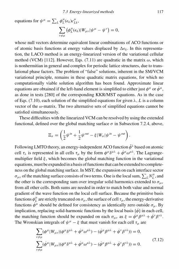
7.3 Energy-linearized methods 117
equations for ψµ =∑L φ
µ
L (εk)cµLk ,∑ν �=µ
(φµ
L (εk)|Wµν |ψµ − ψν) = 0,
whose null vectors determine equivalent linear combinations of ACO functions orof atomic basis functions at energy values displaced by �εk . In this representa-tion, the LACO method is an energy-linearized version of the variational cellularmethod (VCM) [112]. However, Eqs. (7.11) are quadratic in the matrix ω, whichis nonhermitian in general and complex for periodic lattice structures, due to trans-lational phase factors. The problem of “false” solutions, inherent in the SM/VCMvariational principle, remains in these quadratic matrix equations, for which nocomputationally viable solution algorithm has been found. Approximate linearequations are obtained if the left-hand element is simplified to either just φµ or φµ,as done in tests [280] of the corresponding KKR/MST equations. As in the caseof Eqs. (7.10), each solution of the simplified equations for given λ, L is a columnvector of the ω-matrix. The two alternative sets of simplified equations cannot besatisfied simultaneously.
These difficulties with the linearized VCM can be resolved by using the extendedfunctional, defined over the global matching surface σ in Subsection 7.2.4, above,
�σ =(
1
2ψ in + 1
2ψout − ξ |Wσ |ψ in − ψout
).
Following LMTO theory, an energy-independent ACO function φλ based on atomiccell τλ is represented in all cells τµ by the form φµδµλ + φµωµλ. The Lagrange-multiplier field ξ , which becomes the global matching function in the variationalequations, must be expanded in a basis of functions that can be extended to complete-ness on the global matching surface. In MST, the expansion on each interface sectorσµν of the matching surface consists of two terms. One is the local sum,
∑L NµL , and
the other is the corresponding sum over irregular solid harmonics extended to σµνfrom all other cells. Both sums are needed in order to match both value and normalgradient of the wave function on the local cell surface. Because the primitive basisfunctionsφµL are strictly truncated onσµ, the surface of cell τµ, the energy-derivativefunctions φµ should be defined for consistency as identically zero outside σµ. Byimplication, replacing solid-harmonic functions by the local basis {φ} in each cell,the matching function should be expanded on each σµν as ξ = φµβµλ + φνβνλ.The Wronskian integrals of ψµ − ξ that must vanish for each cell τµ are∑
ν �=µ(φµ|Wµν |(φµδµλ + φµωµλ)− (φµβµλ + φνβνλ)) = 0,
(7.12)∑ν �=µ
(φµ|Wµν |(φµδµλ + φµωµλ)− (φµβµλ + φνβνλ)) = 0.

118 7 Multiple scattering theory for molecules and solids
If the total number of basis functions φµL for all cells is Nφ , then for each globalsolution index λ there are 2Nφ equations for the 2Nφ elements of the column vectorsωµλ and βµλ. Thus the variational equations derived from �σ provide exactly thenumber of inhomogeneous linear equations needed to determine the two coefficientmatrices, ω and β. These equations have not yet been implemented, but theypromise to provide an internally consistent energy-linearized full-potential MST.
7.4 The Poisson equation
For a solid or molecule subdivided into atomic cells, the Poisson equation, givenin Rydberg units by
∇2v = −8πρ, (7.13)
can be solved by full-potential multiple scattering theory methods. Here ρ is thelocal number density of electrons, and the negative electronic charge is factoredout of both charge density and potential. Adopting the classical theory of inhomo-geneous linear differential equations to a cellular model, particular solutions arefirst obtained for each atomic cell and then modified by the addition of regularsolutions of the homogeneous equation to satisfy continuity and boundary condi-tions. The original full-potential MST [432] was modified for the Poisson equationand applied to a periodic charge distribution on an fcc space-lattice [247]. In thisexample all atomic cells are geometrically equivalent, so the actual calculation isfor a single cell with periodic boundary conditions. The given charge distribution,with Heaviside cutoff factors at the polyhedral cell boundary, was expanded inspherical harmonics at radii up to that of the enclosing sphere. A local particu-lar solution v0 was obtained by integrating equations analogous to the KKR/MSTequations in spherical polar coordinates, subject to the boundary condition that theparticular solution should vanish at large r . The external continuation of v0 is asum of multipole potentials. Within a particular cell, the sum of these potentialsdue to all other cells defines a local potential �v, expressed in terms of structureconstants that are just the coefficients in the two-center expansion of the Coulombinteraction. �v is added to v0 to give the required global solution of the Poissonequation. The surface integral MST method described below has been applied to thePoisson equation, and is incorporated in the LACO program package [278], stillusing structure constants. More recently, MST cellular methods, using direct match-ing theory with NVCM (GFCM) and JVCM equations rather than structure con-stants, were applied to this problem in a detailed numerical study [443]. This studyfinds that the JVCM is the most accurate and reliable of the methods considered,which included standard MST with structure constants.

7.4 The Poisson equation 119
Multiple scattering theory treats the Poisson equation as an inhomogeneousHelmholtz equation of zero energy (Laplace equation). The Green function G0
is proportional to the Coulomb potential. In Rydberg units, 8πG0 = −2/r12. Aparticular solution v0 and complementary solution �v within a local atomic cell τare defined by subdividing the Lippmann–Schwinger equation such that
v = v0 +�v = −8π∫τ
G0ρ − 8π∫R3−τ
G0ρ. (7.14)
The choice of solid-harmonic functions
JL = r �YL/(2�+ 1); NL = r−�−1YL
gives the well-known one-center expansion of 1/r12 [188]. It is assumed that thelocal density function is subdivided into spherical harmonic components as ρ =∑
L ρL . Each of these components defines a particular solution within the enclosingsphere of the local cell. A very efficient numerical algorithm is available for solvingthe radial Poisson equation [229], generalized to arbitrary �-values [278]. Denotingthese primitive solutions by vL , the ACO construction can be used to define aparticular solution v0L for each ρL such that v0L = vL −
∑J c in the local cell τ .
v0L matches onto an external function∑
Ns on the cell surface σ . The coefficientmatrices here are defined by
cL ′,L = (NL ′ |Wσ |vL ), sL ′,L = −(JL ′ |Wσ |vL ). (7.15)
The complementary potential �v or generalized Madelung term is expanded inregular solid harmonics as
�vµ
L = −∑
L ′JµL ′�cµL ′,L . (7.16)
The coefficients here are
�cµ = −∑ν
gµν(J ν |Wν |vν0
), (7.17)
obtained by substituting the two-center expansion of Nµ into the second term inEq. (7.14), or, equivalently, into
∑Ns.
Alternative equations for the coefficients �c are given by direct matching atcellular interfaces, bypassing the need for structure constants. The two alternativesconsidered by [443] are the NVCM or GFCM equations,∑
ν �=µ(Nµ|Wµν |J ν)�cν −�cµ =
∑ν �=µ
(Nµ|Wµν |vν0
), (7.18)

120 7 Multiple scattering theory for molecules and solids
and the JVCM equations,∑ν �=µ
(Jµ|Wµν |J ν)�cν =∑ν �=µ
(Jµ|Wµν |vν0
)− (Jµ|Wµ|vµ0). (7.19)
Exploiting the high efficiency of the integration algorithm for the radial Poissonequation [229], MST surface integral formalism [274, 278] reduces the computationof multipole moments of cellular charge densities to the evaluation of Wronskiansurface integrals. Electrostatic multipole moments QL are defined by the asymp-totic external potential for each cell τ . For the particular choice of solid-harmonicfunctions given above,
lim r→∞v0L =∑
NL ′ sL ′,L = −8π∑
L
NL QL . (7.20)
A factor−2 included in the last term here compensates for the use of Rydberg unitsand for the omission of the negative electronic charge in potential functions derivedfrom Eq. (7.14). Hence the electrostatic multipole moments of atomic cell τµ are
QµL = −1
8π
∑L ′
sµL ,L ′ =1
8π
(JµL |Wσµ |
∑L ′vµ
L ′
). (7.21)
This equation is used for � = 0 to evaluate normalization integrals in the LACOprogram package [278], avoiding numerical volume quadrature.
7.5 Green functions
Although electronic structure calculations are usually concerned with finding theeigenfunctions ψi (x) and eigenvalues εi of the Schrodinger equation, the corre-sponding Green function is required for many classes of applications. Problemsdealing with impurities, transport, disordered systems, photoemission, etc. are mostnaturally solved using the Green function. In principle, the Green function can beconstructed from eigenfunctions, using the spectral representation,
G(x, x′) =∑
i
ψi (x)(ε − εi )−1ψ∗i (x′).
This representation converges very slowly in general, and an alternative methodis needed. Direct methods for computing the Green function are considered here,using boundary-matching methods of multiple scattering theory. An importantconsideration, in the context of extensions and applications of density functionaltheory (DFT), is that any external perturbing potential will in general be modified orscreened by a self-consistent response. Hence any incremental potential consideredhere is assumed to be modified or screened in the sense of linear-response theory[79, 292].

7.5 Green functions 121
7.5.1 Definitions
For energy κ2 in Rydberg units, the Green function of the Helmholtz equation, withgiven boundary conditions, satisfies
(∇2 + κ2)G0(x, x′) = δ(x, x′), (7.22)
while the corresponding Schrodinger Green function satisfies
(∇2 + κ2 − v(x))G(x, x′) = δ(x, x′). (7.23)
These two Green functions are related by the Lippmann–Schwinger integralequation
G(x, x′) = G0(x, x′)+∫�3
G0(x, y)v(y)G(y, x′)d3y. (7.24)
The wave function of a perturbed system defined by �v(x) is
ψ(x) = ψ(x)+∫�3
G(x, x′)�v(x′)ψ(x′)d3x′. (7.25)
This equation can be applied to a wide class of problems including the electronicstructure of vacancies, impurities, and of other localized perturbations of solids andatomic clusters. The methods considered here make it possible to construct G(x, x′)for any potential function v(x) defined throughout the coordinate space �3.
It is assumed that �3 is subdivided into space-filling cells. A typical cell τµ hasclosed surface σµ. An external empty cell can be included to fill space for a finitesystem. Solutions of the homogeneous Helmholtz equation about the origin of cellµdefine regular and irregular generalized solid-harmonic functions, denoted here byJµL and NµL , respectively. Each generalized solid-harmonic function is the productof a radial factor and a spherical-harmonic function, defined here by a combinedindex L that denotes the quantum numbers (�m). Normalization is assumed to beconsistent with the Kronecker-delta relation,
(NL |Wσ |JL ′) = δL ,L ′ . (7.26)
Expressed in local coordinates for each atomic cell, the Helmholtz Green functioncan be expanded in solid-harmonic functions,
G0(r, r′) = −∑
L
JL (r)N ∗L (r′), r < r ′. (7.27)
To verify this expansion, consider G0(r, r′) for a fixed point r′. For r < r ′, thisfunction is a regular solution of the Helmholtz equation and must have an expansion

122 7 Multiple scattering theory for molecules and solids
of the form
G0(r, r′) =∑
L
JL (r)(NL |W0|G0), (7.28)
where the Wronskian integral is over the surface of any sphere centered at the cellorigin with radius r0 < r ′. For r > r ′, this function is a bounded solution of theHelmholtz equation and must have an expansion of the form
G0(r, r′) = −∑
L
NL (r)(JL |W1|G0), (7.29)
where the Wronskian integral is over the surface of any sphere centered at thecell origin with radius r1 > r ′. If Eq. (7.22) is multiplied by N ∗
L (r), and the cor-responding null term with the Helmholtz operator applied to N ∗
L is subtracted, onintegrating over the volume defined by r0 < r ′ < r1, between radii r0 and r1, thisintegral reduces to Wronskian surface integrals. This implies
N ∗L (r′) = (NL |W1|G0)− (NL |W0|G0). (7.30)
Since r1 > r ′, Eq. (7.29) implies that the first integral on the right-hand side van-ishes. The second integral gives the coefficient in Eq. (7.28), which reduces toEq. (7.27). Similarly, if Eq. (7.22) is multiplied by J ∗L (r) and integrated over thevolume between radii r0 and r1,
J ∗L (r′) = (JL |W1|G0)− (JL |W0|G0). (7.31)
In this case, the second integral on the right-hand side vanishes and the first integralgives the coefficient in Eq. (7.29). This provides a formula valid for r > r ′, com-plementary to Eq. (7.27). Comparison of these two formulas shows that the linearoperator G0 is Hermitian for real energies.
When coordinate x = Xµ + r lies in cell τµ and x′ = Xν + r′ lies in a differentcell τν , a two-center expansion of the Green function is needed. Since NµL (x′ − Xµ)is a regular solution of the Helmholtz equation in a sphere of radius |Xµ − Xν |about the origin of a displaced cell ν,
NµL (r′ + Xν − Xµ) = NµL (r′)δµν −∑
L ′J νL ′(r
′)gνµL ′,L , (7.32)
for r ′ < |Xµ − Xν |. The expansion coefficients gνµL ′,L are structure constants at thegiven energy. This matrix is Hermitian for real energies. Using the above expansion,the Helmholtz Green function can be written in the form,
G0(Xµ + r,Xν + r′) =∑L L ′
JµL (r)gµνL L ′ Jν∗L ′ (r′)−
∑L
JµL (r)N ν∗L (r′)δµν, (7.33)

7.5 Green functions 123
where r < r ′ within any single cell µ. The two-center expansion converges in gen-eral for muffin-tin geometry, when the two coordinate values lie within nonover-lapping spheres. It is assumed here that cell coordinate origins are chosen to satisfythis geometric condition for some neighborhood of each cell origin.
These definitions can be generalized to give an expansion of the Green functionG(x, x′) in terms of local solutions of the Schrodinger equation in each cell τ . Localregular solutions φL and local irregular solutions ζL can be defined by matching tofunctions JL and NL , respectively, on an infinitesimal sphere about the cell origin,or, alternatively, by requiring similar conditions on a local cell boundary σ . Thisconstruction imposes the Wronskian condition
(ζL |Wσ |φL ′) = δL ,L ′ . (7.34)
These integrals vanish between any two φ or two ζ functions. Green’s theoremimplies that this Kronecker-delta formula is valid for Wronskian integrals overany closed surface that encloses the local cell center and excludes all other singularpoints of the potential function. If singularities of the potential function occur only atcell centers, these functions can be assumed to be have regular extensions out to thenearest neighbor cell center, but in general no further. For this reason, the primitivefunction ζ must be modified by the addition of a sum of regular functions φ in itscell of origin to define a modified irregular function ζ that is regular everywhereexcept at the defining cell center. With these definitions [53, 441, 444], by analogyto the Helmholtz Green function,
G(r, r′) = −∑
L
φL (r)ζ ∗L (r′), r < r ′, (7.35)
ζµ
L (r′ + Xν − Xµ) = ζµL (r′)δµν −∑
L ′φνL ′(r
′)GνµL ′,L , (7.36)
for r ′ < |Xµ − Xν |, and
G(Xµ + r,Xν + r′) =∑
L
∑L ′φµ
L (r)GµνL ,L ′φν∗L ′ (r
′)−∑
L
φµ
L (r)ζ ν∗L (r′)δµν, (7.37)
valid for r < r ′ within a single cell, or for coordinates in two nonoverlappingspheres. The coefficients GµνL ,L ′ define the structural matrix of the Schrodinger Greenfunction. For ν = µ, ζ µ − ζµ is a sum of regular functions φµ with coefficients−GµµL ,L ′ .
The definition of irregular functions ζ depends on boundary conditions imposedon the Green function. Any variation of the set of functions ζ defined by addinglinear combinations of the regular functions φ with coefficients that constitute anHermitian matrix simply moves the corresponding term between the two summa-tions in Eq. (7.37), leaving the net sum invariant, and preserving the Kronecker-delta

124 7 Multiple scattering theory for molecules and solids
conditions of Eq. (7.34). The present derivations are covariant with respect to thegroup of such transformations. For particular applications, the representation can bechosen for the greatest convenience, subject only to the Kronecker-delta condition.
7.5.2 Properties of the Green function
The definition of the Schrodinger Green function can be extended to a complex-valued energy parameter z. Then Eq. (7.23) for the Schrodinger equation can bewritten as
(z −H(x))G(z; x, x′) = δ(x, x′), (7.38)
which defines G(z) = (z −H)−1 as the resolvent operator. G(z) is an analytic op-erator function in the upper half of the complex z-plane. The singularities are polesor a continuum branch cut corresponding to energy eigenvalues. If H is Hermitian,the eigenvalues lie on the real energy axis. The corresponding orthonormal set ofeigenfunctions ψi defines a spectral representation
G(z; x, x′) =∑
i
ψi (x)(z − εi )−1ψ∗i (x′). (7.39)
This formula indicates that the residue of G(z) at an eigenvalue pole is just thedensity matrix, in the coordinate representation, summed over all eigenfunctionswith this eigenvalue. This residue can be extracted conveniently by using Dirac’sformula after displacing each eigenvalue into the lower complex plane,
lim δ→01
z − εi + iδ= P 1
z − εi− iπδ(z − εi ). (7.40)
Specializing to the electronic density for electrons of one spin in the local coordi-nates of a particular cell, the local density per unit energy is
n(ε; r) = − 1
π�G(ε; r, r). (7.41)
Summing over all eigenenergies below a chemical potential or Fermi level µ, thelocal density function is defined by a contour integral passing above all poles onthe real axis,
ρ(r) = − 1
π
∫ µ
−∞�G(z; r, r) dz. (7.42)
In methodology based on computation of the Green function, this formula re-places the usual sum over eigenfunctions. When integrated over coordinate space,

7.5 Green functions 125
Eq. (7.41) gives the density of states per unit energy,
n(ε) = − 1
π
∫R3�G(ε; r, r) dτ. (7.43)
These formulas must be summed over a spin index to give the corresponding totaldensities. In multiple scattering theory, the Green function as given by Eq. (7.37) issubdivided into terms valid in separate atomic cells. The elements with r′ = r aresingle sums over the cells. Hence the density of states of given spin in a particularcell τµ is
nµ(ε) = − 1
π
∫τµ
�Gµ(ε; r, r), (7.44)
where Gµ denotes the terms with ν = µ in Eq. (7.37).
7.5.3 Construction of the Green function
Equation (7.24) suggests that the structural matrix GµνL ,L ′ of the Schrodinger Greenfunction at specified energy should have a simple relationship to that of theHelmholtz Green function, which is the matrix of structure constants gµνL ,L ′ . Thebasis set of regular local solutions of the Schrodinger equation can be constructedso that matrix G depends only on g and the t-matrix. In deriving the KKR/MSTequations, primitive basis functions were defined by outward integration, startingfrom specified regular solid-harmonic functions JL at the origin in each atomiccell. A canonical basis set is defined by transforming the primitive basis by ma-trix C−1, where CL ,L ′ is defined as in MST. Hence, in the canonical basis, C isa unit matrix. The matching equations on the local cell boundary depend only onthe t-matrix, because each basis function matches to a boundary function J − Nt .These basis functions, still indexed by L , are in one-to-one correspondence withthe regular solid-harmonic functions JL . Corresponding to the canonical regularbasis function φL , which matches onto J − Nt on cell surface σ , a paired canoni-cal irregular function ζL can be computed by integrating the Schrodinger equationinwards from σ , starting from a single irregular function NL on this surface. Thefull set of canonical basis functions satisfies Eq. (7.34).
The structural matrix G can be derived in this canonical basis from the matrix g ofstructure constants, using the surface-matching theorem. For a modified irregularfunction ζ λ and the corresponding global matching function ξ = 'µNµβµ, thematching conditions on the boundary of any cell τµ are(
JµL |Wµσ |ζ λ − ξ
) = 0,(NµL |Wµ
σ |ζ λ − ξ) = 0. (7.45)
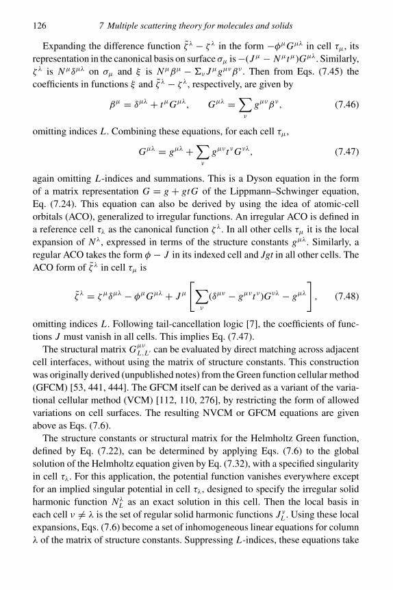
126 7 Multiple scattering theory for molecules and solids
Expanding the difference function ζ λ − ζ λ in the form −φµGµλ in cell τµ, itsrepresentation in the canonical basis on surface σµ is−(Jµ − Nµtµ)Gµλ. Similarly,ζ λ is Nµδµλ on σµ and ξ is Nµβµ −'ν Jµgµνβν . Then from Eqs. (7.45) thecoefficients in functions ξ and ζ λ − ζ λ, respectively, are given by
βµ = δµλ + tµGµλ, Gµλ =∑ν
gµνβν, (7.46)
omitting indices L . Combining these equations, for each cell τµ,
Gµλ = gµλ +∑ν
gµν tνGνλ, (7.47)
again omitting L-indices and summations. This is a Dyson equation in the formof a matrix representation G = g + gtG of the Lippmann–Schwinger equation,Eq. (7.24). This equation can also be derived by using the idea of atomic-cellorbitals (ACO), generalized to irregular functions. An irregular ACO is defined ina reference cell τλ as the canonical function ζ λ. In all other cells τµ it is the localexpansion of N λ, expressed in terms of the structure constants gµλ. Similarly, aregular ACO takes the form φ − J in its indexed cell and Jgt in all other cells. TheACO form of ζ λ in cell τµ is
ζ λ = ζµδµλ − φµGµλ + Jµ[∑ν
(δµν − gµν tν)Gνλ − gµλ], (7.48)
omitting indices L . Following tail-cancellation logic [7], the coefficients of func-tions J must vanish in all cells. This implies Eq. (7.47).
The structural matrix GµνL ,L ′ can be evaluated by direct matching across adjacentcell interfaces, without using the matrix of structure constants. This constructionwas originally derived (unpublished notes) from the Green function cellular method(GFCM) [53, 441, 444]. The GFCM itself can be derived as a variant of the varia-tional cellular method (VCM) [112, 110, 276], by restricting the form of allowedvariations on cell surfaces. The resulting NVCM or GFCM equations are givenabove as Eqs. (7.6).
The structure constants or structural matrix for the Helmholtz Green function,defined by Eq. (7.22), can be determined by applying Eqs. (7.6) to the globalsolution of the Helmholtz equation given by Eq. (7.32), with a specified singularityin cell τλ. For this application, the potential function vanishes everywhere exceptfor an implied singular potential in cell τλ, designed to specify the irregular solidharmonic function N λL as an exact solution in this cell. Then the local basis ineach cell ν �= λ is the set of regular solid harmonic functions J νL . Using these localexpansions, Eqs. (7.6) become a set of inhomogeneous linear equations for columnλ of the matrix of structure constants. Suppressing L-indices, these equations take
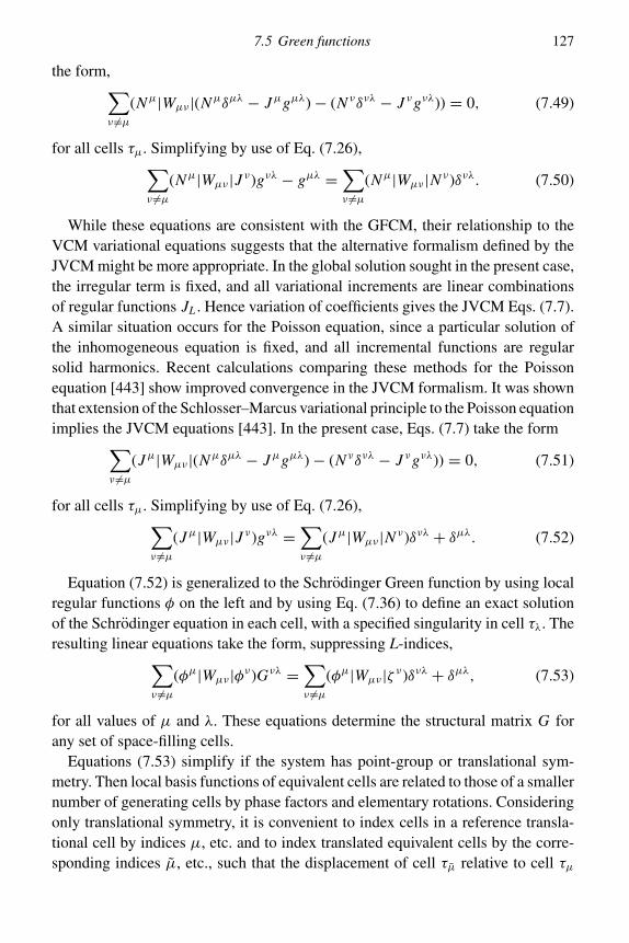
7.5 Green functions 127
the form,∑ν �=µ
(Nµ|Wµν |(Nµδµλ − Jµgµλ)− (N νδνλ − J νgνλ)) = 0, (7.49)
for all cells τµ. Simplifying by use of Eq. (7.26),∑ν �=µ
(Nµ|Wµν |J ν)gνλ − gµλ =∑ν �=µ
(Nµ|Wµν |N ν)δνλ. (7.50)
While these equations are consistent with the GFCM, their relationship to theVCM variational equations suggests that the alternative formalism defined by theJVCM might be more appropriate. In the global solution sought in the present case,the irregular term is fixed, and all variational increments are linear combinationsof regular functions JL . Hence variation of coefficients gives the JVCM Eqs. (7.7).A similar situation occurs for the Poisson equation, since a particular solution ofthe inhomogeneous equation is fixed, and all incremental functions are regularsolid harmonics. Recent calculations comparing these methods for the Poissonequation [443] show improved convergence in the JVCM formalism. It was shownthat extension of the Schlosser–Marcus variational principle to the Poisson equationimplies the JVCM equations [443]. In the present case, Eqs. (7.7) take the form∑
ν �=µ(Jµ|Wµν |(Nµδµλ − Jµgµλ)− (N νδνλ − J νgνλ)) = 0, (7.51)
for all cells τµ. Simplifying by use of Eq. (7.26),∑ν �=µ
(Jµ|Wµν |J ν)gνλ =∑ν �=µ
(Jµ|Wµν |N ν)δνλ + δµλ. (7.52)
Equation (7.52) is generalized to the Schrodinger Green function by using localregular functions φ on the left and by using Eq. (7.36) to define an exact solutionof the Schrodinger equation in each cell, with a specified singularity in cell τλ. Theresulting linear equations take the form, suppressing L-indices,∑
ν �=µ(φµ|Wµν |φν)Gνλ =
∑ν �=µ
(φµ|Wµν |ζ ν)δνλ + δµλ, (7.53)
for all values of µ and λ. These equations determine the structural matrix G forany set of space-filling cells.
Equations (7.53) simplify if the system has point-group or translational sym-metry. Then local basis functions of equivalent cells are related to those of a smallernumber of generating cells by phase factors and elementary rotations. Consideringonly translational symmetry, it is convenient to index cells in a reference transla-tional cell by indices µ, etc. and to index translated equivalent cells by the corre-sponding indices µ, etc., such that the displacement of cell τµ relative to cell τµ

128 7 Multiple scattering theory for molecules and solids
is a lattice translational vector dµµ. Using this notation, Eqs. (7.53) imply separateequations for each k-vector in the reduced Brillouin zone, in the form∑
ν �=µ(φµ|Wµν |φν) exp(ik · dνν )Gνλ(k) =∑ν �=µ(φµ|Wµν |ζ ν) exp(ik · dνν)δνλ + δµλ, (7.54)
for all values of µ and λ that index cells in the reference translational cell. Thecorresponding equations derived from Eq. (7.50) have been verified by comput-ing structure constants for an fcc lattice along the ( − K line in the reducedBrillouin zone, checked against a published structure-constant program STR [384].Equations (7.53) have not been tested, but are expected to show improved conver-gence because they are variationally correct for this problem.
8
Variational methods for continuum states
The principal references for this chapter are:
[3] Adhikari, S.K. (1998). Variational Principles and the Numerical Solution ofScattering Problems (Wiley, New York).
[47] Burke, P.G. and Robb, W.D. (1975). The R-matrix theory of atomic processes, Adv.At. Mol. Phys. 11, 143–214.
[178] Huo, W.M. and Gianturco, F.A. (1995). Computational Methods for Electron-Molecule Collisions (Plenum, New York).
[202] Kohn, W. (1948). Variational methods in nuclear collision problems, Phys. Rev. 74.1763–1772.
[214] Lane, A.M. and Thomas, R.G. (1958). R-matrix theory of nuclear reactions, Rev.Mod. Phys. 30, 257–353.
[215] Lane, N.F. (1980). The theory of electron–molecule collisions, Rev. Mod. Phys. 52,29–119.
[246] Moiseiwitsch, B.L. (1966). Variational Principles (Interscience, New York).[257] Mott, N.F. and Massey, H.S.W. (1965). The Theory of Atomic Collisions (Oxford
University Press, New York).[270] Nesbet, R.K. (1980). Variational Methods in Electron-Atom Scattering Theory
(Plenum, New York).[371] Schwinger, J. (1947). A variational principle for scattering problems, Phys. Rev. 72,
742.[428] Wigner, E.P. and Eisenbud, L. (1947). Higher angular momenta and long range
interaction in resonance reactions, Phys. Rev. 72, 29–41.
8.1 Scattering by an N-electron target system
Scattering by an N-electron atom or molecule with fixed nucleus is described byan (N+1)-electron Schrodinger wave function of the form
!s =∑
p
A#pψps +∑µ
"µcµs . (8.1)
The index s here denotes a particular degenerate solution, specified by boundaryconditions, at given total energy E . The N-electron function#p is a target state with
129

130 8 Variational methods for continuum states
energy E p. It is assumed that all target functions #p are defined by orthonormaleigenvectors of a Hamiltonian matrix in a common set of N-electron basis functions.The eigenvalues are the energies E p. ψps is a one-electron channel orbital wavefunction, antisymmetrized into #p by the operator A. The functions "µ are anorthonormal set of (N+1)-electron Slater determinants. The channel orbital ψps
is characterized by orbital and spin angular momentum quantum numbers and byasymptotic energy E − E p. This energy is positive for open scattering channels,defining a wave vector or electron momentum kp such that E − E p = 1
2 k2p. Hartree
atomic units are used here. If E − E p < 0 the channel is closed. Then kp is replacedby iκp, for κp > 0. In practice, the basis functions "µ are replaced by symmetry-adapted linear combinations of simple Slater determinants, defined for total spinand atomic orbital angular momentum or for molecular point-group symmetry. Theexpansion indicated in Eq. (8.1) remains completely general. For heavy atoms, thenotation can be adapted to j j-coupling.
For an atom, or outside a sphere that completely encloses a target molecule,channel orbital functions are of the form
ψps = r−1 f ps(r )Y�m�(θ, φ)ums ,
where, for r →∞, f ps(r ) ∼ k− 1
2p sin(kpr − 1
2�pπ + ηp), for single-channel scat-tering by a neutral target. This functional form must be modified for long-rangeCoulomb and dipole potentials. The normalization implies unit radial flux den-sity for a free electron. For interacting scattering channels, the multichannel wavefunctions are
f ps(r ) ∼ k− 1
2p
[sin
(kpr − 1
2�pπ
)α0ps + cos
(kpr − 1
2�pπ
)α1ps
]. (8.2)
The coefficient matrices α0 and α1 determine scattering matrices and cross sections.Closed-channel orbital functions must vanish for r →∞, in a way determinedby the long-range potentials in the Schrodinger equation. The term in exp(−κpr )implied by analytic continuation of an open-channel orbital through the continuumthreshold is generally dominated by terms in reciprocal powers of r due to suchlong-range potentials.
It is assumed that ψps is orthogonal to all orbital functions used to construct#p and "µ. This ensures that Eq. (8.1) describes projection of !s onto orthog-onal target-state components !p = A#pψps and a residual orthogonal compo-nent !Q =
∑µ "µcµs that is quadratically integrable. The coefficients cµs are
determined variationally. For any calculation using a finite orbital basis, the open-channel termsA#pψps remain distinct from the Hilbert-space component!Q . Theoscillatory function ψps with nonvanishing asymptotic amplitude cannot be repre-sented as a finite superposition of quadratically integrable functions. In contrast,

8.1 Scattering by an N-electron target system 131
closed-channel terms can be included in either sum. In the close-coupling formal-ism, part of!Q can be replaced by A#γψγ s , where#γ represents a target pseudo-state with energy Eγ > E , corresponding to a closed channel. Such a function liesin the electronic continuum. Polarization response can be represented in terms ofsuch polarization pseudostates #γ (p), computed as the first-order perturbation of#p by a polarizing field. The corresponding closed-channel orbital function ψγ s
may be computed from the close-coupling equations derived here.Using the projection-operator formalism of Feshbach [115, 116], an implicit vari-
ational solution for the coefficients cµs in!Q can be incorporated into an equivalentpartitioned equation for the channel orbital functions. This is a multichannel variantof the logic used to derive the correlation potential operator vc in orbital-functionaltheory. Define a projection operator Q such that
!Q = Q!s =∑µ
"µ("µ|!s),
and the orthogonal complement operator P , such that
!P = P!s �∑
p
A#pψps .
Defining a Schrodinger functional � = (!|H − E |!), the Euler–Lagrange equa-tions for fixed energy E are
δ�
δ!∗P= 0;
δ�
δ!∗Q= 0.
The resulting coupled (N+1)-electron equations are
P(H − E)P!P + PHQ!Q = 0
QHP!P + Q(H − E)Q!Q = 0.
The reduced operator Q(H − E)Q in the Q-space can be inverted to give a formalsolution of the second equation,
!Q = −{Q(H − E)Q}−1QHP!P .
The operator {Q(H − E)Q}−1 is an (N+1)-electron linear operator whose kernelis ∑
µ,ν
"µ(H − E)−1µν"
∗ν.
When substituted into the first equation, this gives an effective multichannelSchrodinger equation of the form
{H − E}!P = {P(H − E)P − PHQ{Q(H − E)Q}−1QHP}!P = 0. (8.3)

132 8 Variational methods for continuum states
Equation (8.3) provides a common basis for the major computational methods usedin low-energy electron scattering theory. The terms containing {Q(H − E)Q}−1 inthis equation describe polarization response and other correlation effects in termsof a matrix optical potential. Singularities due to this energy denominator cancelout exactly [264, 265, 270].
Effective one-electron equations for the channel orbital functions can be obtainedeither by evaluating orbital functional derivatives of the variational functional �or more directly by projecting Eq. (8.3) onto the individual target states #p. Withappropriate normalizing factors, (#p|!s) = ψps . Equations for the radial channelfunctions f ps(r ) are obtained by projecting onto spherical harmonics and elemen-tary spin functions. The matrix operator acting on channel orbitals is
m pq = (#p|H − E |A#q). (8.4)
The projection of this operator onto spherical harmonics and spin functions definesa radial operator m pq = g pq − εpδpq , where εp = E − E p.
8.1.1 Cross sections
If there are no open channels at energy E, there are no linearly independent degen-erate solutions of the Schrodinger equation. Each solution !s is characterized bya vector of coefficients αi ps , for i = 0, 1, defined by the asymptotic form of themultichannel wave function in Eq. (8.1). The rectangular column matrix α consistsof the two no × no coefficient matrices α0, α1. Any nonsingular linear combinationof the column vectors of α produces a physically equivalent set of solutions. Whenmultiplied on the right by the inverse of the original matrix α0, the transformedα-matrix takes the canonical form
α0 = I, α1 = K ,
which defines the reactance matrix K = α1(α0)−1. For exact solutions of theprojected Schrodinger equation, the open-channel K-matrix is real and sym-metric [257, 302]. It can be diagonalized by an orthogonal transformation todefine eigenchannels, defined by the eigenvectors. The eigenvalues are tan ησ , forσ = 1, . . . , no, which defines the eigenphases ησ up to a multiple of π radians. Thescattering matrix S is defined by [257]
S = (I + i K )(I − i K )−1,
and the transition matrix T is defined by
T = 1
2i(S − I ) = K (I − i K )−1.

8.1 Scattering by an N-electron target system 133
In terms of eigenchannels and eigenphases,
K ps =no∑σ=1
x pσ xsσ tan ησ
Sps =no∑σ=1
x pσ xsσ exp(2iησ )
Tps =no∑σ=1
x pσ xsσ exp(iησ ) sin(ησ ).
The S-matrix is unitary and symmetric, while the T-matrix is symmetric. Thisparticular definition of the T-matrix reduces for scattering by a central potential tothe phase-shift factor in the scattering amplitude,
f (θ ) = 1
k
∞∑�=0
(2�+ 1) exp(iη�) sin η�P�(cos θ ),
such that the differential cross section is
dσ
d)= | f (θ)|2.
If k is in atomic units a−10 , the differential cross section is in units a2
0 per steradian.Differential and total cross sections for multichannel scattering by an atomic tar-get can be derived from general formulas [27, 184]. The partial cross section forscattering from channel q to channel p is
σqp = 4π
k2q
|Tpq |2 = 4π
k2q
∣∣∣∣∑σ
x pσ xqσ exp(iησ ) sin(ησ )
∣∣∣∣2
.
The total cross section for unpolarized scattering is obtained by summing σqp overdegenerate final states and by averaging over initial states.
8.1.2 Close-coupling expansion
If the set of target states#p in Eq. (8.1) could be extended to completeness, solutionof the coupled equations for the channel orbitals ψps would provide a quantitativesolution of the scattering problem for an N-electron target. This is the strategyof the close-coupling method [374, 325, 48, 376]. The coupled integrodifferen-tial equations for the channel orbitals are the close-coupling equations. Becausethe expansion in target states must be truncated for any practical calculation, thesecond term in Eq. (8.1) is required in order to include polarization and correlationeffects as well as to assure consistent orbital orthogonality conditions. No generally

134 8 Variational methods for continuum states
satisfactory way has been found to include the continuum of unbound target statesrequired for completeness of this expansion.
Since only a relatively small number of coupled equations can be solved inpractice, the target states #p must be selected carefully. Virtual target excitationinto the ionization continuum must be approximated by inclusion of closed-channelpseudostates that cannot be target eigenstates but have the character of wave packetsin the continuum. Target polarization response is treated by including polarizationpseudostates #γ (p).
If only a single target state is included, itself represented as a single-determinantmodel state"p, the formalism reduces to the static-exchange (SE) model. Becauseof the complexity of more detailed scattering models, much work in fixed-nucleielectron scattering by molecules has been carried out at this level of approximation[215]. This model is generally unsatisfactory for low-energy scattering, and mustbe augmented by a valid approximation to the dipole polarization response of thetarget system [270, 135]. Models that augment static exchange with polarizationresponse are denoted by the acronym SEP. It will be shown below that a model withthis computational structure can be derived from formally exact orbital functionaltheory (OFT), if the correlation potential operator vc is approximated in terms ofpolarization pseudostates [290].
8.2 Kohn variational theory
Variational theory relevant to the representation of an (N+1)-electron continuumwave function by Eq. (8.1) will be considered here. Direct computational imple-mentation of this formalism defines the matrix variational method. Since the widelyapplied close-coupling method can be described by Eq. (8.1), the general argumenthere also applies to that formalism, with some modifications of detail. In the al-gebraic close-coupling method, the variational formalism, using an orbital basisexpansion, replaces direct numerical solution of integrodifferential close-couplingequations.
In bound-state calculations, the Rayleigh–Ritz or Schrodinger variational princi-ple provides both an upper bound to an exact energy and a stationary property thatdetermines free parameters in the wave function. In scattering theory, the energy isspecified in advance. Variational principles are used to determine the wave functionbut do not generally provide variational bounds. A variational functional is madestationary by choice of variational parameters, but the sign of the residual error is notdetermined. Because there is no well-defined bounded quantity, there is no simpleabsolute standard of comparison between different variational trial functions. Thepresent discussion will develop a stationary estimate of the multichannel K-matrix.Because this matrix is real and symmetric for open channels, it provides the most

8.2 Kohn variational theory 135
convenient of several alternative representations of the asymptotic part of a scatter-ing wave function. Recent developments that exploit aspects of the complex-valuedS- or T-matrices will be discussed below.
Variational principles for scattering matrices and wave functions were originallyintroduced by Hulthen [175, 176] and by Kohn [202]. Quantitative applications ofvariational methods to electron–atom scattering theory began with calculations ofe−–H elastic scattering by Schwartz [369, 370], using the Kohn method for theK-matrix. Further progress required understanding and resolution of the problemof spurious singularities in the Kohn formalism. These developments have beendiscussed in detail elsewhere [270]. More recently, this problem has largely beenbypassed in the complex Kohn formalism, which has been very effectively used forcalculations of electron–molecule scattering [341].
8.2.1 The matrix variational method
The asymptotic form of radial open-channel orbitals f ps(r ) is given by Eq. (8.2).Functions of this form can be represented as linear combinations of two independentcontinuum basis functions for each open channel. These basis functions must beregular at the coordinate origin, but have the asymptotic forms
F0p(r ) ∼ k− 1
2p sin
(kpr − 1
2�pπ
),
(8.5)
F1p(r ) ∼ k− 1
2p cos
(kpr − 1
2�pπ
).
A variational approximation with the required asymptotic form
f ps(r ) = F0pα0ps + F1pα1ps (8.6)
determines the coefficients αi ps defined by Eq. (8.2). In the matrix variationalmethod [270], the quadratically integrable orbital basis is augmented for each openchannel by adding two functions φ0p, φ1p whose radial factors are r−1 F0p(r ) andr−1 F1p(r ), respectively. These functions are orthogonalized to the quadraticallyintegrable orbital basis {φi ;φa}.
For an exact scattering wave function, the coefficients cµs in Eq. (8.1) wouldbe determined as linear functions of the matrix elements αi ps , since the algebraicequations are linear. By factoring these coefficients
cµs =∑
i p
cipµ αi ps,

136 8 Variational methods for continuum states
the variational approximation to the (N+1)-electron wave function takes the form
!s =∑
i p
(A#pφi p +
∑µ
"µcipµ
)αi ps .
In the matrix variational method, the coefficients cipµ are determined separately
for each set of indices i, p from the matrix equations, for all µ,("µ|H − E |A#qφ jq +
∑ν
"νcjqν
)= 0, (8.7)
which imply the variational condition ("µ|H − E |!s) = 0. For arbitrary values ofthe coefficients αi ps these equations follow from the variational condition
∂�st
∂cip∗µ
= 0,
for all µ, i, p. The variational functional �st = (!s |H − E |!t ) here is an no × no
matrix.When Eq. (8.7) is satisfied, the variational functional becomes an explicit
quadratic function of the coefficientsαi ps , which can be assumed to be real numbers.Thus
�st =∑
i p
∑jq
αi psm pqi j α jqt ,
where, as a consequence of Eq. (8.7),
m pqi j = M pq
i j −∑µ,ν
Mip,µ(M−1)µνMν, jq .
This equation combines several submatrices of H − E : the Hermitian bound–boundmatrix Mµν , the rectangular bound–free matrix Mµ,i p, and the nonhermitian free–free matrix M pq
i j , where
Mµν = ("µ|H − E |"ν),Mµ,i p = ("µ|H − E |A#pφi p),
M pqi j = (A#pφi p|H − E |A#qφ jq).
Phase factors can be chosen so that both M pqi j and m pq
i j are real but unsymmetrical.If !t were an exact solution of the Schrodinger equation, and total energy E is
above the thresholds for no open channels, there would be no linearly independentsolutions of the equations ∑
jq
m pqi j α jqt = 0, (8.8)

8.2 Kohn variational theory 137
for all indices i, p. Each such solution defines a 2no element column vector ofthe rectangular matrix of coefficients α. In a matrix notation, suppressing channelindices, the variational functional is
� = α†mα = α†0(m00α0 + m01α1)+ α†1(m10α0 + m11α1).
In this notation, Eq. (8.8) is
mα =(
m00 m01
m10 m11
)(α0
α1
)= 0.
The reactance matrix K is α1α−10 . Exact solutions require the matrix m pq
i j to be ofrank no, implying no linearly independent null-vectors as solutions of the homo-geneous equations mα = 0. Because this algebraic condition is not satisfied ingeneral by approximate wave functions, a variational method is needed in order tospecify in some sense an optimal approximate solution matrix α.
If α were an exact solution of the matrix equation mα = 0, the functional � =α†mα would vanish. For a variational approximation, consider the variation of �induced by an infinitesimal variation δα. This is
δ� = δα†mα + (mα)†δα + α†(m − m†)δα.
The last term here does not vanish even if mα = 0. The nonhermitian part of m pqi j
comes from the free–free matrix of H − E , which is characteristic of scattering the-ory. When channel orbital functions are normalized to unit flux, with the asymptoticforms specified above, this nonhermitian term is given by
m pqi j − mqp
ji = M pqi j − Mqp
ji =1
2δpq(δi0δ j1 − δi1δ j0).
This formula expresses the surface integral obtained by integrating the kinetic en-ergy integral by parts for open-channel orbital functions of the specified asymptoticform. In matrix notation,
m01 − m†10 =
1
2I,
where I is the no × no unit matrix. The matrices m00 and m11 are Hermitian (realand symmetric). When substituted into the expression for δ� this gives
δ� = δα†mα + (mα)†δα + 1
2(α†0δα1 − α†1δα0). (8.9)
8.2.2 The Hulthen–Kohn variational principle
Although δ� does not vanish even if the variational equation mα = 0 is satisfied,the nonvanishing terms can be combined with variations of the various scattering
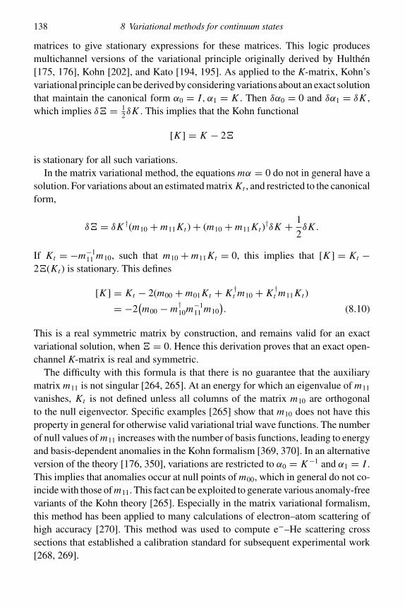
138 8 Variational methods for continuum states
matrices to give stationary expressions for these matrices. This logic producesmultichannel versions of the variational principle originally derived by Hulthen[175, 176], Kohn [202], and Kato [194, 195]. As applied to the K-matrix, Kohn’svariational principle can be derived by considering variations about an exact solutionthat maintain the canonical form α0 = I, α1 = K . Then δα0 = 0 and δα1 = δK ,which implies δ� = 1
2δK . This implies that the Kohn functional
[K ] = K − 2�
is stationary for all such variations.In the matrix variational method, the equations mα = 0 do not in general have a
solution. For variations about an estimated matrix Kt , and restricted to the canonicalform,
δ� = δK †(m10 + m11 Kt )+ (m10 + m11 Kt )†δK + 1
2δK .
If Kt = −m−111 m10, such that m10 + m11 Kt = 0, this implies that [K ] = Kt −
2�(Kt ) is stationary. This defines
[K ] = Kt − 2(m00 + m01 Kt + K †t m10 + K †
t m11 Kt )
= −2(m00 − m†
10m−111 m10
). (8.10)
This is a real symmetric matrix by construction, and remains valid for an exactvariational solution, when � = 0. Hence this derivation proves that an exact open-channel K-matrix is real and symmetric.
The difficulty with this formula is that there is no guarantee that the auxiliarymatrix m11 is not singular [264, 265]. At an energy for which an eigenvalue of m11
vanishes, Kt is not defined unless all columns of the matrix m10 are orthogonalto the null eigenvector. Specific examples [265] show that m10 does not have thisproperty in general for otherwise valid variational trial wave functions. The numberof null values of m11 increases with the number of basis functions, leading to energyand basis-dependent anomalies in the Kohn formalism [369, 370]. In an alternativeversion of the theory [176, 350], variations are restricted to α0 = K−1 and α1 = I .This implies that anomalies occur at null points of m00, which in general do not co-incide with those of m11. This fact can be exploited to generate various anomaly-freevariants of the Kohn theory [265]. Especially in the matrix variational formalism,this method has been applied to many calculations of electron–atom scattering ofhigh accuracy [270]. This method was used to compute e−–He scattering crosssections that established a calibration standard for subsequent experimental work[268, 269].

8.2 Kohn variational theory 139
8.2.3 The complex Kohn method
The derivation given above of the stationary Kohn functional [K ] depends onlogic that is not changed if the functions F0 and F1 of Eq. (8.5) are replaced ineach channel by any functions for which the Wronskian condition m01 − m†
10 =12 I is satisfied [245, 191]. The complex Kohn method [244, 237, 440] exploitsthis fact by defining continuum basis functions consistent with the canonical formα0 = I, α1 = T , where T is the complex-symmetric multichannel transition matrix.These continuum basis functions have the asymptotic forms
u0p(r ) ∼ k− 1
2p sin
(kpr − 1
2�pπ
),
u1p(r ) ∼ k− 1
2p exp i
(kpr − 1
2�pπ
).
This transformed representation of the asymptotic wave functions can easily beverified for potential scattering. The asymptotic radial wave function in a given�-channel satisfies the identity
k−12 eiη sin
(kr − 1
2�π + η
)= k−
12
[sin
(kr − 1
2�π
)+ ei(kr− 1
2 �π )T
],
where T = (e2iη − 1)/2i = eiη sin η.Using these asymptotic continuum functions, the derivation given above implies
that for Tt = −m−111 m10, such that m10 + m11Tt = 0, then
[T ] = Tt − 2�(Tt ) = −2(m00 − m†
10m−111 m10
)is stationary for infinitesimal variations of Tt , and for infinitesimal variations aboutan exact solution for which � = 0. The significance of this revised formalism isthat the matrix m11, constructed from complex exponential basis functions, is asymmetric matrix but no longer real. Its null values are displaced away from thereal energy axis, which essentially eliminates the problem of Kohn anomalies [237].This can be rationalized from the theory of scattering resonances: null values of m11
correspond to pure outgoing-wave solutions of the projected Schrodinger equation.This condition characterizes resonances that in general are displaced below the realenergy-axis by a finite width or reciprocal lifetime [192, 382].
Introduced in the context of heavy-particle reactive collisions [440], the complexKohn method has been successfully applied to electron–molecule scattering [341].It is accurate but computationally intensive, since continuum basis orbitals do nothave the Gaussian form that is exploited in most ab initio molecular bound-statestudies. The method has been implemented using special numerical methods [341]developed for these integrals. These numerical methods mitigate another practical

140 8 Variational methods for continuum states
limitation of the matrix variational method [270], in that analytic formulas areavailable only for specialized forms of the long-range potentials that can occur,especially for molecules.
8.3 Schwinger variational theory
In the Hulthen–Kohn formalism of the matrix variational method, a large partof the computational effort is concerned with the evaluation and inversion of thebound–bound matrix of the (N+1)-electron operator H − E . Because powerfulcomputational methods for this matrix can be taken over directly from bound-stateatomic physics and theoretical chemistry, there is a great practical advantage inusing continuum variational methods that incorporate this as a central aspect of theoverall algorithm. A fundamentally different approach replaces the Schrodingerequation by a formally equivalent Lippmann–Schwinger integral equation [228],developing stationary expressions for the resulting scattering matrices. In suchmethods, a Green function is introduced for the asymptotic electron continuumpart of the overall wave function, while short-range effects are treated through anincremental potential �v. This formalism makes use of the Schwinger variationalprinciple [371]. Formulated as a variational method using exponential or Gaussianorbital basis functions [419, 418], and extended to a multichannel formalism [270,396], it has been widely applied to calculations of electron–molecule scattering[230, 177].
The theory will be developed here with reference to a spherical coordinate system,appropriate to a target atom or to a single-center representation of a molecular wavefunction. Extension to a multicenter representation is straightforward, followingthe same formal argument, but greatly complicates the notation and the detailedform of the Green function used in this theory. The formalism can most easily beunderstood in the simple model of potential scattering in a single �-channel. A modelSchrodinger equation, determined by a radial Hamiltonian operator h = t + v(r ),is assumed to be modified by a difference potential �v, which may be a nonlocallinear operator. At energy ε = 1
2 k2, in the scattering continuum, regular and irregularsolutions w0(r ) and w1(r ), respectively, of the model equation
(h − ε)wi (r ) = 0
are assumed to be known. If normalized to unit Wronskian,
w1(r )w′0(r )− w′1(r )w0(r ) = 1,
these functions define a Green function G, a linear operator whose kernel is
g(r, r ′) = 2w0(r<)w1(r>).

8.3 Schwinger variational theory 141
Acting on any function F(r ) that vanishes for r →∞ and is regular at the originr → 0,
G F(r ) = 2
[w0(r )
∫ ∞
rw1(r ′)+ w1(r )
∫ r
0w0(r ′)
]F(r ′) dr ′.
This implies that (h − ε)G F = F , which can be verified by applying the operatorh − ε to G F(r ). Thus the Green function is a formal inverse of h − ε. The kernelfunction g(r, r ′) is symmetric in r, r ′, regular at the origin in either variable, andcontinuous. The derivative in either variable is discontinuous at r ′ = r , so that(h − ε)G is equivalent to a Dirac δ-function. G depends on ε by construction.
G F ∼ 2w0(r )∫ ∞
0w1(r ′)F(r ′) dr ′
at the coordinate origin, r → 0, and as r →∞,
G F ∼ 2w1(r )∫ ∞
0w0(r ′)F(r ′) dr ′.
Thus G F is regular at the origin but is asymptotically proportional to the irregu-lar function w1(r ). It has the properties assumed for the second continuum basisfunction required for each open channel in the matrix variational method.
These properties of the model Green function imply that the Lippmann–Schwinger equation [228],
f = w0 − G�v f,
defines a solution of the radial Schrodinger equation (h − ε +�v) f (r ) = 0. Reg-ular and irregular functions with asymptotic forms, respectively,
w0 ∼ k−12 sin
(kr − 1
2�π
)a, w1 ∼ k−
12 cos
(kr − 1
2�π
),
are used to construct the principal value Green function. This Green function im-poses the asymptotic form f (r ) ∼ w0(r )+ w1(r ) tan η, where
tan η = −2∫ ∞
0w0(r ′)�v(r ′) f (r ′) dr ′.
Other asymptotic forms consistent with unit Wronskian define different but equallyvalid Green functions, with different values of the asymptotic coefficient of w1. Inparticular, if w1 ∼ k−
12 exp i(kr − 1
2�π ), this determines the outgoing-wave Greenfunction, and the asymptotic coefficient of w1 is the single-channel T-matrix,eiη sin η. This is the basis of the T-matrix method [342, 344], which has beenused for electron–molecule scattering calculations [126]. It is assumed that �v fis regular at the origin and that �v vanishes more rapidly than r−2 for r →∞.

142 8 Variational methods for continuum states
Coulomb or static dipole potentials should be included in the model potential whosesolutions w0, w1 are used to construct the Green function.
Specializing the present derivation to the principal value Green function, theunsymmetrical expression tan η = −2(w0|�v| f ) is exact for an exact solution ofthe Lippmann–Schwinger equation, but it is not stationary with respect to infinites-imal variations about such a solution. Since w0 = f + G�v f for such a solution,this can be substituted into the unsymmetrical formula to give an alternative, sym-metrical expression tan η = −2( f |�v +�vG�v| f ), which is also not stationary.However, these expressions can be combined to define the Schwinger functional
[tan η] = −2(w0|�v| f )( f |�v +�vG�v| f )−1( f |�v|w0),
which is stationary for variations of the trial function f about an exact solution.The variation δ[tan η] induced by an infinitesimal variation of f about an exactsolution is [
(δ f |�v|w0)
( f |�v|w0)− (δ f |�v +�vG�v| f )
( f |�v +�vG�v| f )+ hc
][tan η]
= −2(δ f�v|w0 − f − G�v f )+ hc.
This implies that [tan η] is stationary if and only if f , in the range of �v, satisfiesthe Lippmann–Schwinger equation.
The Schwinger functional has several remarkable properties. It combines threeformulas that may have different numerical values:
tan η � −2(w0|�v| f ),
tan η � −2( f |�v +�vG�v| f ),
tan η � −2( f |�v|w0).
The function f can be arbitrarily normalized, because [tan η] is homogeneous inf . There is no constraint on the asymptotic form of trial functions, because theyhave no effect outside the range of the assumed short-range potential �v. Onlythe regular model functionsw0 occur explicitly in the theory, although the irregularfunctionsw1 must be consistent with the asymptotic character of the Green function,and may be used to construct it.
An algebraic theory is obtained if f is expanded within the range of �v as alinear combination f (r ) =∑
a ηa(r )(a| f ) of orthonormal basis functions {ηa}.�vis expanded in the same basis as a linear integral operator with the kernel,
�v(r, r ′) =∑a,b
ηa(r )�vabη∗b(r ′).
For [tan η] to be stationary with respect to variations of the coefficients (a| f ), this

8.3 Schwinger variational theory 143
requires, for all indices a,
(a| f − w0 + G�v f ) = 0.
This is a system of linear equations that determine
(a| f ) =∑
b
(I + G�v)−1ab (b|w0)
=∑b,c
(�v +�vG�v)−1ab�vbc(c|w0).
Combining these equations, all three expressions for tan η give the same result forthe stationary functional,
[tan η] =∑a,b
∑c,d
(w0|a)�vac(�v +�vG�v)−1cd �vdb(b|w0).
8.3.1 Multichannel Schwinger theory
For practical use in electron scattering theory, the Lippmann–Schwinger equationand the Schwinger variational principle must be generalized to a multichannelformalism. In applying this formalism, the orthogonality conditions that distin-guish the bound and free components of an (N+1)-electron continuum !s , asgiven in Eq. (8.1), must be taken into account. The argument here summarizesan earlier derivation [270]. The multichannel close-coupling equations appropri-ate to the (N+1)-electron problem require orthogonality constraints expressed byoff-diagonal Lagrange multipliers. Reduction to a form in which these parametersvanish by construction will be considered here after generalizing the Schwingerstationary principle to such equations in their simpler homogeneous form.
Consider the multichannel radial close-coupling equations, without Lagrangemultipliers for orthogonality, ∑
q
m pquqs(r ) = 0, (8.11)
where
m pq = (h − ε)pq +�v pq .
It is assumed that all closed-channel components have been eliminated by thepartitioning transformations that determine Eq. (8.4), from which the radial operatorm pq is derived. Equations of this form can be solved using the Green function ofthe model problem ∑
s
(h − ε)pswisq(r ) = 0.

144 8 Variational methods for continuum states
The multichannel model functions w0sq and w1sq are real-valued continuum solu-tions of the model problem, in a K-matrix formalism. They are normalized to thematrix Wronskian condition∑
s
(w′ispw jsq − wispw′jsq) = δpq(δi0δ j1 − δi1δ j0).
The equations here are simplified by working in an eigenchannel representation,in which the model K-matrix is diagonalized, with eigenvalues tan ησ . Definingmatrices C and S, diagonal in the eigenchannel representation, with eigenvaluescos ησ and sin ησ , respectively, the physical K-matrix implied by an incrementalmatrix K ′ in this representation is [375]
K = (S + C K ′)(C − SK ′)−1.
The multichannel generalization of the principal value Green function is a linearoperator Gσpq , defined by its kernel
gσpq(r, r ′) = 2w0pσ (r<)w1qσ (r>),
indexed by eigenchannel σ of the model continuum functions.If {Fq(r )} is a vector of functions, one for each open channel, that are regular at
the coordinate origin and quadratically integrable, then∑q
Gσpq Fq(r ) =∑
q
2
{w0pσ (r )
∫ ∞
rw1qσ (r ′)+ w1pσ (r )
∫ r
0w0qσ (r ′)
}Fq(r ′) dr ′,
such that ∑σ
∑p,q ′
(h − ε)pp′Gσp′q Fq(r ) = Fp(r ).
Using the matrix Wronskian condition, the proof is the same as for the single-channel problem.
This multichannel matrix Green function determines a multichannel Lippmann–Schwinger equation
u pτ = w0pτ −∑σ
∑p′,q
Gσpp′�vp′quqτ
that determines solutions of the multichannel Schrodinger equation. The asymptoticform of the second term here is
−2∑p,q
w1pσ (w0pσ |�v pq |uqτ ),
which implies that the incremental K-matrix in the model eigenchannel representa-tion is K ′ = −2(w0|�v|u), in a matrix notation. The Hermitian conjugate relationis K ′ = −2(u|�v|w0).
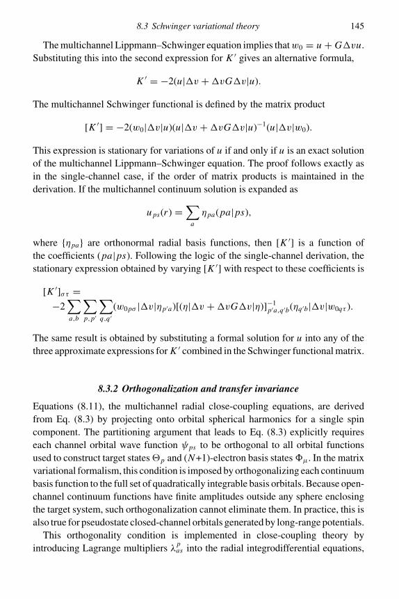
8.3 Schwinger variational theory 145
The multichannel Lippmann–Schwinger equation implies thatw0 = u + G�vu.Substituting this into the second expression for K ′ gives an alternative formula,
K ′ = −2(u|�v +�vG�v|u).
The multichannel Schwinger functional is defined by the matrix product
[K ′] = −2(w0|�v|u)(u|�v +�vG�v|u)−1(u|�v|w0).
This expression is stationary for variations of u if and only if u is an exact solutionof the multichannel Lippmann–Schwinger equation. The proof follows exactly asin the single-channel case, if the order of matrix products is maintained in thederivation. If the multichannel continuum solution is expanded as
u ps(r ) =∑
a
ηpa(pa|ps),
where {ηpa} are orthonormal radial basis functions, then [K ′] is a function ofthe coefficients (pa|ps). Following the logic of the single-channel derivation, thestationary expression obtained by varying [K ′] with respect to these coefficients is
[K ′]στ =−2
∑a,b
∑p,p′
∑q,q ′
(w0pσ |�v|ηp′a)[(η|�v +�vG�v|η)]−1p′a,q ′b(ηq ′b|�v|w0qτ ).
The same result is obtained by substituting a formal solution for u into any of thethree approximate expressions for K ′ combined in the Schwinger functional matrix.
8.3.2 Orthogonalization and transfer invariance
Equations (8.11), the multichannel radial close-coupling equations, are derivedfrom Eq. (8.3) by projecting onto orbital spherical harmonics for a single spincomponent. The partitioning argument that leads to Eq. (8.3) explicitly requireseach channel orbital wave function ψps to be orthogonal to all orbital functionsused to construct target states#p and (N+1)-electron basis states"µ. In the matrixvariational formalism, this condition is imposed by orthogonalizing each continuumbasis function to the full set of quadratically integrable basis orbitals. Because open-channel continuum functions have finite amplitudes outside any sphere enclosingthe target system, such orthogonalization cannot eliminate them. In practice, this isalso true for pseudostate closed-channel orbitals generated by long-range potentials.
This orthogonality condition is implemented in close-coupling theory byintroducing Lagrange multipliers λp
as into the radial integrodifferential equations,

146 8 Variational methods for continuum states
which become ∑q
m pquqs(r ) =∑
a
ηpaλpas . (8.12)
The λmultipliers are determined by the orthogonality condition. If the quadraticallyintegrable radial basis in channel p is the orthonormal set {ηpa}, values of theLagrange multipliers are given by
λpas =
∑q
(ηpa|m pq |u ps).
In the Lippmann–Schwinger formalism, the Green function can be defined in aprojected orbital space consistent with this orthogonality condition. An alternative,assumed in the derivation given above, is to use a Green function appropriate toclose-coupling equations from which the Lagrange multipliers have been elimi-nated. This can be done if each (N+1)-electron trial wave function has the propertyof transfer invariance [270]. This means that !s , in Eq. (8.1), is unchanged underany transfer of quadratically integrable terms A#pφps between its free and boundcomponents,
∑p A#pψps and
∑µ "µcµs , respectively. If a valid system of close-
coupling equations exists for any arbitrary transfer of such terms, these equationsare transfer covariant. Projection of the Schrodinger equation onto the bound spacedetermines the coefficients cµs through linear equations
("µ|H − E |!s) = 0
for all µ, or ∑ν
(H − E)µνcνs = −∑
p
("µ|H − E |A#pψps).
This is transfer covariant if all quadratically integrable functions are representedin the same orbital basis. Requiring ψps to be orthogonal to all φpa (radial factorηpa(r )) enforces a unique representation, but introduces Lagrange multipliers inthe close-coupling equations. An alternative is to require
(#p|H − E |!s) = 0
to be valid for all #p, and to adjust the Lagrange multipliers accordingly. Thisimplies that
(A#pφpa|H − E |!s) = 0
for all p, a. This reduces to∑q
(ηpa|m pq |uqs) = λpas = 0,

8.4 Variational R-matrix theory 147
which removes the Lagrange multipliers, if the operator m pq is determined from(#p|H − E |!s) as in the matrix variational formalism. This analysis shows that arepresentation of the transfer-covariant close-coupling equations exists in which theLagrange multipliers for orthogonalization vanish. This representation is assumedin the development of the multichannel Schwinger theory given above.
Use of the model Green function in the Lippmann–Schwinger equation is the mostserious weakness of the Schwinger variational formalism. The method requires�vto be a short-range potential or operator, so that it can be represented quantitativelyin a quadratically integrable orbital basis. This requires all long-range potentialsto be included in the model Hamiltonian used to construct the Green function.This is a formidable difficulty in the context of electron–molecule scattering, sincemuch of the structure of low-energy cross sections is due to polarization responseand to long-range dipole and quadrupole potentials [215, 178]. A molecular Greenfunction must satisfy Coulomb cusp conditions and be regular at each atomic center,precluding the use of standard asymptotic forms for model long-range potentials.Construction of such a Green function and evaluation of the implied integrals(η|�vG�v|η) requires analytic or computational methodology beyond presentcapabilities.
8.4 Variational R-matrix theory
The Wigner–Eisenbud [428] R-matrix, or derivative matrix, is defined by the rela-tionship between radial channel orbitals f ps(r ) and their derivatives on some sphereof radius r1 that surrounds a target system [214, 33]. Assuming spherical geometry,the dimensionless radial R-matrix Rpq at r1 is defined by
f ps(r1) =∑
q
Rpqr1 f ′qs(r1).
The indices refer to both open and closed channels, which do not have to be dis-tinguished at the finite radius r1. As defined for solutions of radial close-couplingequations, Rpq is a real symmetric matrix. Extension of the theory and definitions tomore general geometry will be considered below. For electron–molecule scattering,a molecular center is chosen somewhat arbitrarily such that the electronic chargeis approximately enclosed in some smaller sphere of radius r0, while bound–freeexchange can be neglected outside the larger R-matrix radius r1.
The theory of the R-matrix was developed in nuclear physics. As usually pre-sented, the theory makes use of a Green function to relate value and slope of theradial channel orbitals at r1, expanding these functions for r < r1 as linear com-binations of basis functions that satisfy fixed boundary conditions at r1. The truelogarithmic derivative (or reciprocal of the R-matrix in multichannel formalism)

148 8 Variational methods for continuum states
is computed from Green’s theorem, despite the use of basis functions whose log-arithmic derivatives at r1 have a fixed but arbitrary value. Because of the inherentdiscontinuity of the boundary derivative this expansion tends to converge slowly,and requires correction by an approximate method due to Buttle [54].
In nuclear physics, the specifically nuclear interaction is of short range, so thatfull scattering information is obtained by matching the R-matrix at r1 to asymptoticexternal wave functions. The method has been extended to electron–atom scatter-ing, where long-range potentials are important, by combining basis expansion ofthe channel orbital functions within r1 with explicit numerical solution of close-coupling equations outside [50, 47]. This method makes it possible to processalgebraic equations defined by matrix elements of nonlocal operators within r1,while solving the simple asymptotic close-coupling equations, without exchange,outside r1. This requires r1 to be large enough that exchange can be neglectedand that the nonlocal optical potential can be approximated by an asymptotic localpotential.
The R-matrix can be matched at r1 to external channel orbitals, solutions inprinciple of external close-coupling equations, to determine scattering matrices.Radial channel orbital vectors, of standard asymptotic form for the K-matrix,
w0pq(r ) ∼ k− 1
2p sin
(kpr − 1
2�pπ
)δpq,
w1pq(r ) ∼ k− 1
2p cos
(kpr − 1
2�pπ
)δpq,
are defined by integrating inwards for r > r1. The asymptotic forms must be modi-fied appropriately for Coulomb or fixed-dipole scattering. The function to be fittedat r1 is
f ps(r1) =∑
q
[w0pq(r1)δqs + w1pq(r1)Kqs].
The R-matrix relation between function value and gradient can be solved for theK-matrix,
Kst = −∑
p
[w1ps(r1)−
∑q
r1 Rpq(r1)w′1qs(r1)
]−1
sp
×[w0pt (r1)−
∑q
r1 Rpq(r1)w′0qt (r1)
]pt
.
As written, these equations refer to open channels only. When external closedchannels are considered, an external closed channel orbital that vanishes as r →∞must be included for each such channel. The indices p, q, s run over all channels,

8.4 Variational R-matrix theory 149
but the index t refers to open channels only. Kst is a rectangular matrix, whoseopen-channel submatrix can be shown to be real and symmetric.
The theory of the R-matrix can be understood most clearly in a variational for-mulation. The essential derivation for a single channel was given by Kohn [202],as a variational principle for the radial logarithmic derivative. If h is the radialHamiltonian operator, the Schrodinger variational functional is
� =∫ ∞
0f (h − ε) f dr.
If f (r ) is an exact solution for r > r1, this reduces the functional to the finite integralconsidered by Kohn,
�λ =∫ r1
0f (h − ε) f dr =
∫ r1
0
[1
2( f ′)2 +
(v(r )− 1
2k2
)f 2
]dr − 1
2λ f 2(r1),
obtained after integration by parts. The parameter λ is the logarithmic derivativef ′/ f = (r1 R)−1, defining the parameter R as the single-channel R-matrix.
For an infinitesimal variation δ f , with fixed λ, the variation of �λ is
δ�λ = 2∫ r1
0δ f (h − ε) f dr + δ f (r1)[ f ′(r1)− λ f (r1)].
This vanishes for unconstrained variations if and only if (h − ε) f = 0 for 0 ≤r ≤ r1 and λ = f ′(r1)/ f (r1).
If f (r ) is approximated by a finite expansion in linearly independent basis func-tions {ηa}, such that f =∑
a ηaca , variation of �λ with respect to the coefficientsca gives the linear equation∑
b
Aabcb = 1
2ληa(r1) f (r1), (8.13)
where
Aab =∫ r1
0
[1
2η′aη
′b + ηa
(v(r )− 1
2k2
)ηb
]dr. (8.14)
The parameter λ is uniquely determined as a consistency condition [202]. FromEq. (8.13),
ca = 1
2λ∑
b
(A−1)abηb(r1) f (r1),
so that
f (r1) =∑
a
ηa(r1)ca = 1
2λ∑a,b
ηa(r1)(A−1)abηb(r1) f (r1).

150 8 Variational methods for continuum states
Unless f (r1) vanishes, this requires as a consistency condition
R = (r1λ)−1 = 1
2r1
∑a,b
ηa(r1)(A−1)abηb(r1),
which is the standard formula for the single-channel R-matrix.Several important aspects of this formula generalize immediately to multichannel
scattering. The matrix Aab is the Hermitian residue of � after integration by parts,which separates off the boundary term as a surface integral. This boundary termdetermines the R-matrix, which contains all information needed to extend an internalsolution by matching to external wave functions. Thus the internal Schrodingerequation, which may contain nonlocal potentials such as an optical potential, issolved by the typical bound-state method of expanding in a set of basis functions,while the external problem may be solved by some completely independent method.If r1 is large enough that asymptotic potentials are valid for r > r1, then specializedand highly efficient analytic methods may be used, without affecting the variationalexpansion appropriate to the inner region.
A multichannel generalization of the variational R-matrix theory was derived byJackson [183]. In the context of the generalized close-coupling equations, incor-porating an optical potential derived by Feshbach partitioning, this is in principlean exact theory. Exact solutions of the coupled equations are assumed for r ≥ r1,determined by specifying their values at r1 in terms of an R-matrix. For each chan-nel p, projected onto spin and spatial symmetry (angular) functions, there are twolinearly independent radial functions. If these are denoted by u0ps(r ) and u1ps(r ),respectively, for a global wave function indexed by s, the boundary conditions atr1 chosen by Jackson are
u0ps(r1) = 0, u′0ps(r1) = δpsr− 1
21
u1ps(r1) = δpsr+ 1
21 , u′1ps(r1) = 0.
In this R-matrix theory, open and closed channels are not distinguished, but theeventual transformation to a K-matrix requires setting the coefficients of expo-nentially increasing closed-channel functions to zero. Since the channel functionssatisfy the unit matrix Wronskian condition, a generalized Kohn variational princi-ple is established [195], as in the complex Kohn theory. In this case the canonicalform of the multichannel coefficient matrices is
α0 = I, α1 = R
and the radial channel orbital function is
f ps(r ) =∑
t
(u0ptδts + u1pt Rts), r ≥ r1.

8.4 Variational R-matrix theory 151
Then, by construction,
f ps(r1) = Rpsr12
1 , f ′ps(r1) = δpsr− 1
21 ,
in agreement with the defining equation for the R-matrix,
f ps(r1) =∑
q
Rpqr1 f ′qs(r1).
Since an exact solution is assumed outside r1, the Schrodinger matrix functionalis
�st =∑p,q
∫ r1
0f †ps(r )m pq fqt (r ) dr,
whose variation is given by Eq. (8.9). This defines a trial R-matrix Rt = −m−111 m10,
such that m10 + m11 Rt = 0 in this representation of the channel orbitals, and impliesthat [R] = Rt − 2�(Rt ) is stationary. This defines
[R] = −2(m00 − m†
10m−111 m10
). (8.15)
This expression is stationary with respect to variations about an exact solution.Because radial derivatives of the functions u1ps all vanish at r = r1, null values of
the determinant of m11 characterize eigensolutions of the multichannel Schrodingerequation that satisfy a homogeneous Neumann boundary condition on the R-matrixsphere. In contrast to the Kohn formalism for the K-matrix, these null values are notanomalous, but are a characteristic feature of any system of integrodifferential equa-tions as energy or other parameters are varied. In one dimension, this simply meansthat the logarithmic derivative passes through zero, as a continuous nondecreasingfunction of energy.
The derivation by Kohn [202] can readily be extended to the multichannelR-matrix. The underlying logic depends on the variational principle that the multi-channel Schrodinger functional is stationary for variations of a trial function thatsatisfies the correct boundary conditions if and only if that function satisfies theSchrodinger equation. In a matrix notation, suppressing summations and indices,the variational functional of Schrodinger is
� =∫
f † A f − 1
2r1f †(r1)R−1 f (r1),
when integrated by parts to separate the surface term from the residual Hermitianvolume term
∫f † A f . Here R is a trial R-matrix, analogous to a Lagrange multiplier,
to be adjusted so that the trial wave function satisfies R-matrix boundary conditions

152 8 Variational methods for continuum states
at r = r1. A defines the modified Hamiltonian operator of Bloch [30], such that
hB − ε = h − ε + 1
2δ(r − r1)
d
dr.
Its representation in an orbital basis {ηa} defines the matrix A given by Eq. (8.14).Given f = ηc, the functional becomes
� = c†[
A − 1
2r1η†(r1)R−1η(r1)
]c.
Variation with respect to the coefficients c†, for fixed R, gives the linear equations
Ac = 1
2r1η†(r1)R−1 f (r1),
whose solution is
c = 1
2r1A−1η†(r1)R−1 f (r1).
This implies that � = 0 and
f (r1) = η(r1)c = 1
2r1η(r1)A−1η†(r1)R−1 f (r1).
Unless A is singular, as it is at the null values of m11, this implies the consistencycondition, restoring summation indices,
Rpq = 1
2r1
∑a,b
ηa(r1)(A−1)pqab η
†b(r1).
Since matrix A is Hermitian by construction, the R-matrix is also Hermitian, andcan be made real by suitable choice of phase factors for the basis functions. Because� vanishes, Rpq is the stationary value of the matrix [R] in the basis {ηa}.
These early derivations [202, 183] have an important feature, not emphasized atthe time, that has subsequently turned out to be of great practical significance. Noconditions are imposed on the basis functions η other than regularity at the coordi-nate origin and linear independence. The nonvariational theory [428], which usesGreen’s theorem, introduces a complete basis set in the interval 0 ≤ r < r1, obtainedas the set of eigenfunctions of some model Hamiltonian, with a fixed boundary con-dition, r1η
′(r1) = bη(r1). Several standard derivations follow this logic [214, 47].If the trial function f (r ) is expanded as a sum of functions all with the same log-arithmic derivative at r1, it must satisfy this same boundary condition. The valueof λ computed from the variational formula in the Kohn theory differs in gen-eral from the imposed value b/r1. Unless the energy parameter is an exact eigen-value of the A-matrix, with this imposed boundary condition, the trial function instandard R-matrix theory has a discontinuous derivative at r1, if the function value

8.4 Variational R-matrix theory 153
is matched at the boundary. This discontinuity leads to slow convergence of thebasis set expansion [187]. Standard procedure is to remove the gradient disconti-nuity by a nonvariational Buttle correction [54]. This methodology has been usedin an extended series of ab initio calculations of atomic [50, 47] and molecular[138, 139, 249] scattering cross sections. An alternative method [106, 220] is toadjust the parameter b iteratively so that it agrees with the computed value of λ.Other calculations have used the variational formalism directly, implemented withorbital basis functions that are not constrained at r1 [310, 311, 299, 298].
The R-matrix radius r1 must be large enough that all nonlocal interactions canbe neglected or replaced by local asymptotic potentials outside it. In electron–molecule scattering, a much smaller target radius r0 can be defined, within whichthe total target electronic density has converged sufficiently to represent molecularmultipole moments and polarizabilities within the overall accuracy of the full scat-tering calculation. In the intermediate region r0 ≤ r ≤ r1, basis orbital functions forthe target system die off exponentially, while external multipole and polarizationresponse potentials are well approximated by their asymptotic forms. This behav-ior has several very important implications for quantitative ab initio calculations.Crucially, orbital basis sets and multiconfiguration expansions adapted to the targetsystem cannot adequately represent the intermediate region. Open-channel orbitalfunctions retain a constant amplitude throughout this region, and closed-channel(polarization pseudostate) orbitals decay as inverse powers of r , not exponentially.The most direct way to represent this region is to add orthogonalized fixed-energycontinuum orbital functions, two for each open channel, to the basis set. Whensuch basis orbitals are orthogonalized to the exponential basis set, this induces anorthogonal projection of the (N+1)-electron variational basis, as indicated in thedefinition of the (N+1)-electron wave function, Eq. (8.1). Fixed linear combinationsof Gaussian basis orbitals (with small exponents) can be constructed that modelspherical Bessel functions or Coulomb functions quite accurately in the inter-mediate region [300]. An alternative basis for the intermediate region is the setof numerical asymptotic functions (NAFs), continuum eigenfunctions of the modelHamiltonian constructed from the long-range asymptotic potential functions, in-tegrated outwards from r0 [311]. Since the centrifugal potential barrier increasesrapidly with orbital angular momentum �, orbital functions with high � values be-come insensitive to the region inside r0. This justifies the asymptotic distorted-wave(ADW) approximation [273], in which the R-matrix is computed by numerical inte-gration of the asymptotic close-coupling equations from r0 to r1. The high-� channelsectors of this matrix are used to augment a variational R-matrix computed in anorbital basis cut off at some relatively smaller �-value. NAF orbitals and the ADWapproximation were used in accurate calculations of fixed-nuclei e−–H2 scatteringcross sections [299, 298].
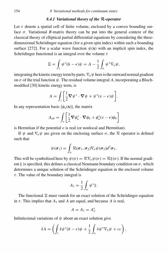
154 8 Variational methods for continuum states
8.4.1 Variational theory of the R-operator
Let τ denote a spatial cell of finite volume, enclosed by a convex bounding sur-face σ . Variational R-matrix theory can be put into the general context of theclassical theory of elliptical partial differential equations by considering the three-dimensional Schrodinger equation (for a given spin index) within such a boundingsurface [272]. For a scalar wave function ψ(x) with an implicit spin index, theSchrodinger functional is an integral over the volume τ
� =∫τ
ψ∗(h − ε)ψ = A − 1
2
∫σ
ψ∗∇nψ,
integrating the kinetic energy term by parts.∇nψ here is the outward normal gradienton σ of the trial functionψ . The residual volume integral A, incorporating a Bloch-modified [30] kinetic energy term, is
A =∫τ
[1
2∇ψ∗ ·∇ψ + ψ∗(v − ε)ψ
].
In any representation basis {φa(x)}, the matrix
Aab =∫τ
[1
2∇φ∗a ·∇φb + φ∗a (v − ε)φb
]
is Hermitian if the potential v is real (or nonlocal and Hermitian).If ψ and ∇nψ are given on the enclosing surface σ , the R operator is defined
such that
ψ(σ1) =∫σ
R(σ1,σ2)∇nψ(σ2)d2σ2.
This will be symbolized here by ψ(σ ) = R∇nψ(σ ) = Rξ (σ ). If the normal gradi-ent ξ is specified, this defines a classical Neumann boundary condition on σ , whichdetermines a unique solution of the Schrodinger equation in the enclosed volumeτ . The value of the boundary integral is
A1 = 1
2
∫σ
ψ∗ξ.
The functional � must vanish for an exact solution of the Schrodinger equationin τ . This implies that A1 and A are equal, and because A is real,
A = A1 = A∗1.
Infinitesimal variations of ψ about an exact solution give
δA =(∫
τ
δψ∗(h − ε)ψ + 1
2
∫σ
δψ∗∇nψ + cc
),
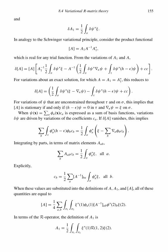
8.4 Variational R-matrix theory 155
and
δA1 = 1
2
∫σ
δψ∗ξ.
In analogy to the Schwinger variational principle, consider the product functional
[A] = A1 A−1 A∗1,
which is real for any trial function. From the variations of A1 and A,
δ[A] = [A]
[A−1
1
1
2
∫σ
δψ∗ξ − A−1
(1
2
∫σ
δψ∗∇nψ +∫τ
δψ∗(h − ε)ψ)+ cc
].
For variations about an exact solution, for which A = A1 = A∗1, this reduces to
δ[A] =(
1
2
∫σ
δψ∗(ξ − ∇nψ)−∫τ
δψ∗(h − ε)ψ + cc
).
For variations of ψ that are unconstrained throughout τ and on σ , this implies that[A] is stationary if and only if (h − ε)ψ = 0 in τ and ∇nψ = ξ on σ .
When ψ(x) =∑a φa(x)ca is expressed as a sum of basis functions, variations
δψ are driven by variations of the coefficients ca . If δ[A] vanishes, this implies
∑b
∫τ
φ∗a (h − ε)φbcb = 1
2
∫σ
φ∗a
(ξ −
∑b
∇nφbcb
).
Integrating by parts, in terms of matrix elements Aab,
∑b
Aabcb = 1
2
∫σ
φ∗aξ, all a.
Explicitly,
cb = 1
2
∑a
[A−1]ba
∫σ
φ∗aξ, all b.
When these values are substituted into the definitions of A, A1, and [A], all of thesequantities are equal to
[A] = 1
4
∑a,b
∫σ1
∫σ2
ξ ∗(1)φa(1)[A−1]abφ∗(2)bξ (2).
In terms of the R-operator, the definition of A1 is
A1 = 1
2
∫σ1
∫σ2
ξ ∗(1)R(1, 2)ξ (2).

156 8 Variational methods for continuum states
Comparison with the stationary value of [A] = A1 indicates that
R(1, 2) = 1
2
∑a,b
φa(1)[A−1]abφ∗b (2).
Because [A] is stationary and the surface function ξ is arbitrary, the operatorR must itself be stationary. It is evidently real and symmetric by construction.The basis functions φa(x) are required only to be linearly independent in τ . En-forcing orthonormality through a fixed boundary condition on σ imposes a lackof completeness with respect to determining the R-operator. The factor 1/r1 isomitted from the definition given above, making the operator R dimensionally alength. This cannot be avoided in general geometry, since no unique radius is de-fined for a nonspherical surface. The usual R-matrix in spherical geometry is thesurface-harmonic representation of the R-operator as defined here, divided by thedimensional scale factor r1.
8.4.2 The R-operator in generalized geometry
In generalized geometry, it may be useful to introduce different coordinate systemson different sectors of a boundary hypersurface σ . This extended definition wasintroduced by Light and Walker [225] to define successive extensions of a prop-agated R-matrix, and implicitly by Schneider et al. [363] in extending R-matrixtheory to vibronic interactions in molecules. It provides the formal basis for recentapplications of adiabatic phase-matrix theory to rovibronic excitation in molecules[284]. It is assumed that coordinates can be defined such that the generalized kineticenergy operator in the enclosed hypervolume τ takes the form
T = 1
2∇ ·∇,
for a generalized scalar product defined by
p · q =∑
i
(1/µi )pi qi .
The R-operator is defined on hypersurface σ by
ψ(σ1) =∫σ
R(σ1,σ2)∇ψ(σ2) · dσ2.
The classical Neumann boundary problem generalizes directly to the hyperspaceif the kinetic energy operator can be put into this canonical form. The argumentgiven above, when generalized to nonspherical geometry, remains valid. Given the

8.4 Variational R-matrix theory 157
normal gradient ξ on σ , the stationary value of the variational functional is
[A] = 1
2
∫σ
∫σ
dσ1ξ∗(σ1)R(σ1,σ2)ξ (σ2) dσ2.
Integration by parts of the Schrodinger functional is equivalent to using a Bloch-modified Schrodinger equation
(HB − E)ψ(x) =∫σ
L(x,σ)ψ(σ) dσ.
Here the Bloch-modified Hamiltonian HB is obtained by integration by parts of thekinetic energy integral,∫
τ
φ∗α Tφβdτ = 1
2
∫τ
∇φ∗α · ∇φβdτ − 1
2
∫σ
φ∗α∇φβ · dσ.
This can be expressed in terms of a Bloch surface operator,
L = 1
2δ(x,σ)n(σ) · ∇
such that
1
2
∫σ
φ∗α∇φβ · dσ =∫τ
φ∗αLφβ dτ.
Expansion in a linear independent orbital basis implies
R(σ1,σ2) = 1
2
∑α
∑β
φα(σ1)(HB − E)−1αβ φ
∗β(σ2).
8.4.3 Orbital functional theory of the R-matrix
Variational R-matrix theory has been developed here in the context of multichannelclose-coupling equations derived by Feshbach partitioning from the (N+1)-electronwave function given by Eq. (8.1). The short-range (exponentially decreasing) part ofthis wave function is eliminated in this formalism, transformed into a multichanneloptical potential in the residual coupled orbital equations. Bound target states andpseudostates have been projected out to define the coupled open and closed “free”electronic channels. These equations take the form of a multichannel generalizationof the ground-state orbital Euler–Lagrange equations of orbital functional theory,derived in Chapter 5 here. This relationship has been used to consider multipolepolarization response as an example of the OFT formalism for electronic correlation[290].

158 8 Variational methods for continuum states
Specializing to electronically elastic scattering, there is only one target referencestate, which will be denoted by", a normalized N-electron Slater determinant con-structed from occupied OFT target orbitals. The target OEL equations are assumedto contain a correlation potential providing an accurate approximation to the trueground state. The (N+1)-electron reference state takes the form A"φκ , where Ais an antisymmetrizing operator. While all bound target orbital functions are nor-malized within the R-matrix boundary r = r1, the continuum orbital φκ extendsbeyond this boundary. Its normalization requires some discussion.
Channel orbital functions are considered here to be orthogonalized to the bound-state orbital basis. If this basis is complete within the target radius r0, these or-thogonalized channel orbitals must effectively vanish inside the target system. InR-matrix formalism, if the effective potentials in the close-coupling equations donot depend on the multichannel orbital functions, these orbitals may be arbitrarilynormalized [270]. Conventionally, they are normalized within the R-matrix volumecharacterized by radius r1, where they are matched to logarithmic derivatives of ex-ternal continuum wave functions normalized to unit flux density. This conventionalnormalization obscures the fact that a continuum orbital, extending throughout aninfinite volume, must vanish in any finite volume if normalized to unity over allspace. In the context of a continuum OFT, a continuum orbital may either be nor-malized to an infinitesimal within the R-matrix boundary or normalized to unitybut assigned an infinitesimal occupation number. The latter option is followed here.In a set of N+1 occupied orbitals, the orbital wave functions are orthonormal forr ≤ r1, but one occupation number nκ → 0+. Thus
∑i ni = N , and bound–free
exchange is described by a Fock operator that depends only on the occupied targetorbitals. Similarly, in the theory developed here, correlation energy of the target isnot affected by a continuum orbital, but bound–free correlation energy acts as aneffective potential for the continuum electron.
In the case of a scattering resonance, bound–free correlation is modified by atransient “bound” state of N+1 electrons. In a finite matrix representation, theprojected (N+1)-electron Hamiltonian H has positive energy eigenvalues, whichdefine possible scattering resonances if they interact sufficiently weakly with thescattering continuum. In resonance theory [270], this transient discrete state ismultiplied by an energy-dependent coefficient whose magnitude is determined bythat of the channel orbital in the resonant channel. Thus the normalization of thechannel orbital establishes the absolute amplitude of the transient discrete state,and arbitrary normalization of the channel orbital cannot lead to an inconsistency.
Bound–free correlation
For an N-electron target state, Ec is a sum of pair-correlation energies. In a two-electron system, such as atomic He, a major contribution to the correlation energy

8.4 Variational R-matrix theory 159
arises from replacement of a product function by one in relative coordinates thatsatisfies the Kato cusp condition at the singularity r12 → 0. In a CI representation,this implies a slowly convergent sum of configurations, including relatively highangular quantum numbers. Methods used to simplify this problem include use ofa free-electron-gas (FEG) local correlation potential [134] and an Ansatz wavefunction that specifically corrects the cusp condition [70]. Complementary to thisshort-range effect, the emphasis here is on long-range correlation potentials thatarise from multipole response of the target to a scattered electron.
The N-electron target wave function is coupled to a continuum orbital φκ forwhich nκ → 0. Vanishing nκ implies that the continuum electron does not modifythe effective Hamiltonian G that acts on occupied target orbitals (ni = 1). G alsoacts on φκ because nκ → 0 cancels out of the functional derivatives in δE
nκ δφ∗κ. This
implies that φκ is orthogonal to the occupied target orbitals. The result is to augmentstandard static-exchange equations with a nonlocal correlation potential vc.
From Eq. (5.7), and Janak’s theorem [185], the contribution of correlation energyto the mean energy of the continuum orbital within the R-matrix boundary is
(κ|vc|κ) =∑
j
n j
∑c<b
(1− nc)(1− nb)(κ j |u|cb)(cb|c|κ j)
−∑k< j
nkn j
∑b
(1− nb)(k j |u|κb)(κb|c|k j), (8.16)
where all integrals are evaluated for r ≤ r1. The second line of this general formulais a correction to target correlation energy due to removal ofφκ from the unoccupiedset. The first line can be shown to include a multipole polarization potential.
To model the effect of close-coupling equations including a closed pseudostatechannel, suppose that a pseudostate orbital φp j represents the first-order pertur-bation of a particular target orbital φ j in a multipole field of order λ, and thatthe pseudostate excitation energy is E p
j − E0. Because φp j is selected to interactstrongly within the inner radius r0, the residual orthogonalized set of unoccupiedorbitals φq remain approximately complete in r0 ≤ r ≤ r1 for functions orthogonalto occupied orbitals. The close-coupling equations imply that a closed-channel or-bital φqκ coupled to φp j is approximately of the form of a slowly decaying functiontimes the open-channel orbital φκ . Hence the average energy of the two-electronvirtual excitations j, κ → p j , q can be approximated by E p
j − E0. This argumentjustifies a closure approximation, and the first line of Eq. (8.16) becomes
(κ|vc|κ) �∑
j
n j
∑q
(1− nq)(κ j |u|qp j )(qp j |c|κ j)
� −∑
j
n j
(κ|( j |u|p j )
(E p
j − E0)−1
(p j |u| j)|κ). (8.17)
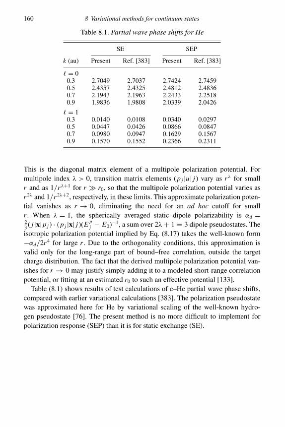
160 8 Variational methods for continuum states
Table 8.1. Partial wave phase shifts for He
SE SEP
k (au) Present Ref. [383] Present Ref. [383]
� = 00.3 2.7049 2.7037 2.7424 2.74590.5 2.4357 2.4325 2.4812 2.48360.7 2.1943 2.1963 2.2433 2.25180.9 1.9836 1.9808 2.0339 2.0426
� = 10.3 0.0140 0.0108 0.0340 0.02970.5 0.0447 0.0426 0.0866 0.08470.7 0.0980 0.0947 0.1629 0.15670.9 0.1570 0.1552 0.2366 0.2311
This is the diagonal matrix element of a multipole polarization potential. Formultipole index λ > 0, transition matrix elements (p j |u| j) vary as rλ for smallr and as 1/rλ+1 for r � r0, so that the multipole polarization potential varies asr2λ and 1/r2λ+2, respectively, in these limits. This approximate polarization poten-tial vanishes as r → 0, eliminating the need for an ad hoc cutoff for smallr . When λ = 1, the spherically averaged static dipole polarizability is αd =23 ( j |x|p j ) · (p j |x| j)(E p
j − E0)−1, a sum over 2λ+ 1 = 3 dipole pseudostates. Theisotropic polarization potential implied by Eq. (8.17) takes the well-known form−αd/2r4 for large r . Due to the orthogonality conditions, this approximation isvalid only for the long-range part of bound–free correlation, outside the targetcharge distribution. The fact that the derived multipole polarization potential van-ishes for r → 0 may justify simply adding it to a modeled short-range correlationpotential, or fitting at an estimated r0 to such an effective potential [133].
Table (8.1) shows results of test calculations of e–He partial wave phase shifts,compared with earlier variational calculations [383]. The polarization pseudostatewas approximated here for He by variational scaling of the well-known hydro-gen pseudostate [76]. The present method is no more difficult to implement forpolarization response (SEP) than it is for static exchange (SE).

9
Electron-impact rovibrational excitation of molecules
The principal references for this chapter are:
[49] Burke, P.G. and West, J.B., eds. (1987). Electron–Molecule Scattering andPhotoionization (Plenum, New York).
[82] Domcke, W. (1991). Theory of resonance and threshold effects in electron–molecule collisions: the projection-operator approach, Phys. Rep. 208, 97–188.
[178] Huo, W.M. and Gianturco, F.A., eds. (1995). Computational Methods for Electron–Molecule Collisions (Plenum, New York).
[215] Lane, N.F. (1980). The theory of electron–molecule collisions, Rev. Mod. Phys. 52,29–119.
[284] Nesbet, R.K. (1996). Nonadiabatic phase-matrix method for vibrational excitationand dissociative attachment in electron–molecule scattering, Phys. Rev. A 54,2899–2905.
[363] Schneider, B.I., LeDourneuf, M. and Burke, P.G. (1979). Theory of vibrationalexcitation and dissociative attachment: an R-matrix approach, J. Phys. B 12,L365–L369.
Electron–molecule scattering data, observed experimentally or computed withmethodology available as of 1980, was reviewed in detail by Lane [215]. If therewere no nuclear motion, electron–molecule scattering would differ from electron–atom scattering only because of the loss of spherical symmetry and because of thepresence of multiple Coulomb potentials due to the atomic nuclei. This is alreadya formidable challenge to theory, exemplified by the qualitative increase in com-putational difficulty and complexity between atomic theory and molecular theoryfor electronic bound states. While bound-state molecular computational methodshave been extended to fixed-nuclei electron scattering [49, 178], an effective andcomputationally practicable treatment of rovibrational (rotational and vibrational)excitation requires a significant and historically challenging extension of bound-state theory. The small ratio between electron and nuclear masses is exploited inbound-state theory through the Born–Oppenheimer separation [31], leading to thequalitative physical principle that in the lowest order of a perturbation expansion,
161
162 9 Electron-impact rovibrational excitation of molecules
transfer of kinetic energy between electronic and nuclear motion can be neglected.In the expansion parameter (m/M)
14 , where M is a typical nuclear mass, elec-
tronic energy is of zeroeth order, vibrational energy of second order, and rotationalenergy of fourth order. Far from neglecting these Born–Oppenheimer corrections,a valid theory of electron-impact rovibrational excitation must compute the scat-tering effects of such terms with quantitative accuracy, because the phenomenonof interest is precisely such an energy transfer between electronic and nuclearmotion.
Rotational level spacing is in fact so small for most molecules that it can beresolved only by precise spectroscopic techniques. Typical electron scattering datadoes not have sufficient energy resolution, and most published data is for rotationallyaveraged scattering cross sections. Special methods based on an adiabatic theoryof slowly moving nuclei are valid under these circumstances, not dependent onvariational theory and methods. However, near excitation or scattering thresholds,rotational analysis may play an essential role in interpreting complex scatteringphenomena due to dynamical long-range potentials, such as the dipole potentialfor heteropolar diatomic molecules, quenched by molecular rotation. For thesereasons, the present discussion of computational methodology will concentrate onthreshold effects characteristic of low-energy electron scattering and on vibrationalexcitation. The phenomenon of dissociative attachment, when an incident electron iscaptured by a target molecule, which then dissociates to produce an ionic fragment,is a particular example of such energy transfer, and will be considered here as anapplication of rovibrational threshold theory.
An electron scattering resonance, in abstract but general mathematical terms, ischaracterized by a singularity of the scattering matrix when analytically continued toa complex energy value εres − i
2γ for relatively small width parameter γ > 0 [270].In simple effective-potential models, a so-called shape resonance occurs when anelectronic energy level in a potential well is degenerate with an energy continuumoutside a potential barrier that confines the well. An electron initially bound inthe state corresponding to this energy level leaks out through the potential barrierwith a time constant h/γ . Such poles of the analytically continued scattering matrixcan also cause significant energy-dependent Wigner cusp or rounded step structures[427, 32] in scattering cross sections just below or just above the energy threshold atwhich a continuum becomes energetically accessible. This behavior is characteristicof long-range potentials and does not require a well-defined potential barrier [270].A typical phenomenon is a virtual state, which occurs in simple potential modelsat the threshold for a continuum with orbital angular momentum � = 0, hence nocentrifugal barrier.
Resonance and threshold structures in fixed-nuclei electron-scattering cross sec-tions are replicated, with characteristic energy shifts, in rovibrational excitation

9.1 The local complex-potential (LCP) model 163
cross sections. One of the most striking examples is provided by the prominentmultiple peaks observed in both the electronically elastic and vibrational excita-tion cross sections for electron scattering by the N2 molecule [368, 143, 95, 215].These peaks are associated with a fixed-nuclei resonance at approximately 2 eV,but their width arises from electron–vibrational coupling and their spacing doesnot correspond precisely to the vibrational level structure of either the neutraltarget molecule or of a vibrating transient negative ion. A quantitative theory ofthese excitation structures has been developed through several advances in bothformalism and computational technique, ultimately based on variational theory ofthe interacting electron–vibrational system. Another striking example is the ob-servation of excitation peaks associated with each successive vibrational excita-tion threshold in electron scattering by dipolar molecules such as HF, HCl, andHBr [346]. Because of the electric dipole moment of such target molecules, iflow-energy scattering theory is to be relevant it must provide a detailed analy-sis of rotational excitation and of rotational screening of the long-range dipolepotential.
9.1 The local complex-potential (LCP) model
Considerable understanding of molecular resonance and threshold phenomena hascome from the conceptually simple model of an electronic resonance state that de-termines a complex-valued effective internuclear potential function, characterizedby a decay width whenever the real part of the resonance energy lies above thefixed-nuclei potential of the target molecule. The vibrational levels of this complexpotential are a first approximation to resonance energies such as those observed inN2. As shown in the “boomerang” model of Herzenberg [167], the implied lifetimeof these model vibrational states is so short that they do not survive a single oscilla-tion of a classical wave packet. Hence a dynamical model arises in which excitationfrom the ground-state vibrational state of the neutral molecule to a wave-packet stateof the transient negative ion is followed by a single vibration out and back, travers-ing a region of relatively long lifetime. Because the decay width increases rapidlyfor small internuclear distances, this wave packet decays into vibrational states ofthe neutral molecule as it makes this return trip, and disappears before completinga full oscillation. With appropriate parametrization, this model gives a convincingexplanation of the observed vibrational resonance peak shapes and separations ine−N2 scattering [24, 91].
The complex-potential model originated as a qualitative explanation of dissocia-tive attachment [18]. A fixed-nuclei electronic resonance is described by a complexpotential whose width goes to zero at the crossing point with the molecular ground-state potential, and remains zero if the resonance potential remains below the target

164 9 Electron-impact rovibrational excitation of molecules
potential for large internuclear separation. In this case, an outgoing wave packetbecomes a true bound state of the negative ion after crossing outwards, and disso-ciates without returning. Excitation and decay processes inside the crossing pointare the same as in the boomerang model. An incident electron, captured into ex-cited ionic vibrational levels, creates a vibronic wave packet that moves outwardswhile decaying into vibrational excitations, but eventually simply crosses outwardsas a molecular negative ion that dissociates into stable fragments. Applied to thedissociative attachment of H2 [16, 19, 415], this parametrized model accuratelyreproduces available experimental data.
A very significant practical problem with the LCP model is the lack of a uniqueand well-defined theory of the required resonance state when its decay width be-comes large. In the case of H−2 , serious discrepancies between various parametrizedor computed values of the energy and width of the 2'+u shape resonance in the LCPmodel of dissociative attachment indicate that a more fundamental, first-principlestheory is needed to give fully convincing results. The difficulty is that as thedecay width becomes large, the concept of a well-defined LCP model becomesquestionable, since the scattering resonance fades into the background scatteringcontinuum [271]. Analytic theory implies an energy shift which may qualitativelychange the character of the assumed resonance potential curve [59, 82].
9.1.1 The projection-operator method
The semiclassical picture of nuclear motion inherent in the LCP model has aquantum-mechanical foundation that is most directly developed in the projection-operator formalism of Feshbach [115, 116, 270]. Domcke [82] reviews the applica-tion of this formalism to resonant effects in electron–molecule scattering. Neglect-ing the kinetic energy of nuclear motion, Tn , an electronic resonance at nuclearcoordinate(s) q is characterized by a pole of the analytically continued scatteringmatrix S(q, ε) at complex energy ε = εres(q)− 1
2 iγ (q), where γ is the decay widthof the resonance. The set of values εres(q) defines the real part of the LCP effec-tive potential curve. The Feshbach formalism in electron–molecule scattering isordinarily applied to the static-exchange model of fixed-nuclei scattering, coupledto the Hamiltonian Hn for nuclear motion [67, 314, 315, 15]. The electronic wavefunction is represented by a model state" (Slater determinant), whose orbital func-tions are orthogonalized to a normalized, localized orbital function φd(q; x) thatinteracts with a continuum orbital wave functionψk to produce the scattering reson-ance. For fixed nuclei, this formalism is exactly the same as resonance theory foratoms, resulting in a complex-valued nonlocal optical potential. It is most directlydescribed by a Green function that is formally orthogonalized to the postulatedlocalized function φd [270, 82].

9.1 The local complex-potential (LCP) model 165
In the LCP model of vibrational excitation, parametrized functions εres(q) andγ (q), together with the ground-state potential curve, V0(q), suffice to determinecross sections averaged over rotational substructure. The full Feshbach formalismrequires parametrized transition matrix elements between φd and orthogonalizedbackground continuum orbitals φk , as well as V0(q) and the mean electronic energyVd(q) of a postulated discrete state φd . In a one-electron model [82], the Feshbachoptical potential is added to the effective electronic Hamiltonian for static exchange.This formalism is readily extended to an orbital-functional theory that includes elec-tronic correlation [290]. The transition element Vdk , parametrized as a function ofboth q and the electronic continuum energy ε, models the (N+1)-electron matrixelement (!d |H |A#0ψk), where !d is a postulated discrete (N+1)-electron state,#0 is the target electronic ground state, and ψk is a continuum orbital functionat energy ε = 1
2 k2. The full function A#0ψk must be orthogonal to !d . Thus theformalism defined by such matrix elements applies to the original case consid-ered by Feshbach, where !d is a core-excited state such as He:(1s3s2)2S at22.45 eV excitation energy, as well as to the explicitly modeled one-electronattached state.
The vibronic Hamiltonian in the one-electron model is H = H0 + V . The kernelsof these operators are
h0 = φd[T n + Vd(q)]φ∗d +∫
k dk d)k φk
[φn + V0(q)+ 1
2k2
]φ∗k ;
v =∫
k dk d)kφd Vdk(q)φ∗k + hc.
The coupled Schrodinger equations can be projected onto the φd · · ·φ∗d subspaceby Feshbach partitioning, giving an equation for the coefficient function χd(q)in the component φdχd(q) of the total wave function. The effective Hamiltonianin this equation is T n + Vd(q)+ Vopt, which contains an optical potential that isnonlocal in the q-space. This operator is defined by its kernel in the φd · · ·φ∗dsubspace,
vopt(q, q′; E) =
∫k dk d)k Vdk(q)
(E − 1
2k2 − T n − V0(q)+ iη
)−1
V ∗dk(q ′).
This defines a nonlocal complex energy shift vopt = �− 12 i( such that
�(q, q ′; E) =∫∑v
∫k dk Vdk(q)χv(q)
[E − 1
2k2 − Ev
]−1
χ∗v (q ′)V ∗dk(q ′),
((q, q ′; E) = 2π∫∑v
Vdkv (q)χv(q)χ∗v (q ′)V ∗dkv (q
′).

166 9 Electron-impact rovibrational excitation of molecules
Here k2v = 2(E − Ev) for the bound or continuum vibrational state indexed by v.
Thus the Feshbach formalism implies energy-dependent, nonlocal energy-shift andwidth functions for a resonance.
Neglecting nonresonant scattering, the resonant contribution to the transitionmatrix is [82]
T (k f , v f ; ki , vi ) =(v f
∣∣V ∗dk f
G(E)Vdki
∣∣vi),
deduced from the Lippmann–Schwinger equation. Here G(E) is the resolventoperator in the φd · · ·φ∗d space,
G(E) = (E − T n − Vd(q)− V opt + iη)−1,
evaluated in the limit η→ 0+ for outgoing-wave boundary conditions. The tran-sition matrix can be computed as
T (k f , v f ; ki , vi ) =(v f
∣∣V ∗dk f
∣∣χd),
since the projected equation for the coefficient function χd(q) implies χd(q) =G(E)Vdkiχvi . This projected equation is
{T n + Vd(q)+ V opt − H}χd(q) = −Vdkiχvi (q), (9.1)
which is nonlocal in the nuclear coordinates [15].Although in earlier applications Vd(q)+ V opt was approximated by an empirical
local complex potential (LCP), more recent work has solved this nonlocal equationdirectly [82], obtaining detailed resonance excitation and near-threshold cross sec-tions in excellent agreement with experimental data. Model calculations, using thenonlocal formalism, indicate that a local approximation can yield accurate results forvibrational excitations [59, 258]. The local model is inadequate for very broad res-onances [259] and for near-threshold singularities [84, 86]. The neglect of nonres-onant scattering implies significant discrepancies for elastic scattering. Despite thepractical success of the projection-operator formalism for resonant scattering, theunderlying electronic theory is still restricted to a static-exchange model, augmentedby an optical potential derived from empirical functions Vd(q) and (d(q) or Vdk(q).
9.2 Adiabatic approximations
The small mass ratio m/M suggests various levels of approximation based funda-mentally on the inherently small kinetic energy of nuclear motion T n . The physicalconcept that justifies the LCP model is that the electronic wave function adjustsessentially instantaneously to displacements of the nuclei, because electronic vel-ocities are much greater than nuclear velocities in a time-dependent semiclassical

9.2 Adiabatic approximations 167
model. Thus nuclear motion is described in an adiabatic picture, assuming instanta-neous electronic relaxation. A more fundamental rationalization can be based on ageneralized independent-particle model, including nuclei as well as electrons. Thisimplies a formally exact theory if electronic correlation and electron–nuclei inter-actions are included. However, the small mass ratio m/M justifies simplificationof the self-consistent mean field that acts on each nucleus even though the nuclearmotion is described by quantum mechanics and T n is treated as a Schrodingeroperator that acts on rovibrational wave functions. Whether or not this mean fieldcan be reduced to a static electronic potential computed for fixed nuclei depends onthe limit of linear response theory for the electrons as m/M → 0. Thus a completequantitative theory must use the full variational theory of interacting electrons, butcan be expected to justify significant simplifications in the treatment of nuclearmotion.
Because molecular rotational kinetic energy and rotational level spacings aresmall in all cases, a rotationally adiabatic model has been widely and successfullyused for electron–molecule scattering [215]. The essence of this adiabatic nuclei(ADN) approximation [313, 63, 64, 401] is that a scattering amplitude or matrixcomputed for fixed nuclei is treated as an operator in the nuclear coordinates. Thenthe rotational state-to-state scattering amplitude or matrix is estimated by matrixelements of this operator in the basis of rotational states. The basic assumption isthat of the Born–Oppenheimer separation: the commutator between the fixed-nucleiscattering operator and the operator T n is neglected. This approximation becomesdifficult to justify only when the precise energy of individual rotational levels isimportant, near thresholds or in the presence of long-range potentials. Because ofthe well-defined internuclear geometry in a body-fixed reference frame, fixed-nucleiscattering matrices are most directly computed in this frame. In contrast, rotationalscattering structure is observed in a fixed laboratory frame. Unless an explicitrotational frame transformation is carried out, strong rotational coupling occurs asa computational artifact [215]. For this reason, applications of the rotational ADNmodel require such a frame transformation [62].
The ADN approximation has been much less successful for vibrational excita-tion, as might be expected from the much larger vibrational level spacings and thestrong variation of fixed-nuclei resonance parameters with nuclear displacements.This motivated the proposal [61] of a hybrid close-coupling model. As appliedto e−N2 vibrational excitation, this model combines fixed-nuclei electronic close-coupling calculations for nonresonant body-frame molecular symmetry states withextended vibronic close-coupling calculations in the 2 g resonant symmetry ofN−2 . Although multipeaked vibrational excitation and vibrationally elastic crosssections are obtained in qualitative agreement with experiment, the peak shapesand spacings are not in good agreement. This can be attributed to truncation of the

168 9 Electron-impact rovibrational excitation of molecules
electronic partial-wave expansion and of the limited number of vibrational statesincluded in the close-coupling basis. A deeper problem is that any complete set ofvibrational states, such as the eigenfunctions of a parametrized Morse potential,must include the vibrational continuum. No practical way has been found to do thisin the close-coupling formalism.
9.2.1 The energy-modified adiabatic approximation (EMA)
In many scattering processes, energy levels of the target system are split by aperturbation that is weak relative to the interaction responsible for the scattering. Theadiabatic approximation neglects the effect on threshold scattering structures andon resonances of the energy-level splitting and energy shifts of the perturbed targetstates. Especially for threshold structures, this can lead to qualitatively incorrectresults. For example, transition matrix elements computed below a rovibrationalexcitation threshold do not vanish if only the fixed-nuclei target energy is takeninto account. This qualitatively incorrect behavior of adiabatic cross sections nearrotational excitation thresholds can be compensated simply by modifying electronmomenta in the adiabatic cross-section formula [64]. With these corrections, theADN theory appears to be adequate for rotational excitation [144].
Much larger anomalous effects occur in vibrational excitation because the energyshifts are larger. The energy-modified adiabatic approximation (EMA) [267] wasintroduced in order to provide a systematic treatment of such effects, while retainingthe computational efficiency of the adiabatic approximation. The usual adiabaticapproximation is modified by allowing for the dependence of unperturbed scat-tering matrices on the kinetic energy of the perturbed target state, using formulasthat are qualitatively correct for threshold and resonance structures. For molecules,this means that for target geometry determined by a generalized coordinate q theenergy ε(q) = E − V (q) of a continuum electron must be replaced in principle byεop(q) = E − Hn(q), an operator in the nuclear coordinates. Fixed-nuclei calcula-tions produce scattering matrices that are functions of numerical parameters q, ε.In the EMA, the integrals that project these matrices onto rovibrational states areevaluated by approximations that replace the parameter ε by the operator εop. Thesimplest such approximation, for diagonal matrix elements in a rovibronic stateindexed by µ, is to replace ε by εµ = E − Eµ. If nondiagonal matrix elementsbetween states indexed by µ and ν are evaluated for the geometric mean energyεµν = [(E − Eµ)(E − Eν)]
12 , this implies correct threshold behavior for general
short-range potentials. When applied to the energy-denominator characteristic of afixed-nuclei molecular resonance, this state-dependent modification of ε to εop wasshown to give qualitatively correct results for the multipeaked vibrational excita-tion structures observed in e−N2 scattering [267]. Because the EMA formalism

9.3 Vibronic R-matrix theory 169
replaces fixed-nuclei scattering matrices by operators that are represented by rovi-bronic scattering matrices, a single fixed-nuclei or threshold structure becomes a setof overlapping scattering structures, displaced with possibly irregular energy shiftsby the discrete vibronic energy level structure of the target molecule [267]. Thisrepetition and displacement of underlying structures is characteristic of observedelectron scattering cross sections for molecular targets. A more recent extension ofthe EMA formalism to the context of variational R-matrix theory is discussed below.
9.3 Vibronic R-matrix theory
Recognizing that exact quantum electron–molecule scattering theory for interactingnuclei and electrons is and will remain computationally intractable, except for thesimplest diatomic molecules, Schneider [361] initiated reconsideration of the Born–Oppenheimer approximation as a logical foundation for the adiabatic nuclei (ADN)formalism. For a long-lived (narrow) resonance, neglect of vibrational derivativesof the fixed-nuclei electronic wave function should be no less valid for electronscattering at low energies than it is for molecular bound states. This argument isthe basis of an electronic R-matrix methodology in which eigenstates, definedby eigenvalues of the Bloch-modified electronic Hamiltonian from which theR-matrix is constructed, are used to define effective molecular potential functions,parametrized by nuclear coordinates [363]. The small mass ratio m/M justifiesneglecting derivatives of the electronic eigenfunctions of this fixed-nuclei Bloch-modified Hamiltonian with respect to the nuclear coordinates.
This work introduced the concept of a vibronic R-matrix, defined on a hyper-surface in the joint coordinate space of electrons and internuclear coordinates. Inconsidering the vibronic problem, it is assumed that a matrix representation ofthe Schrodinger equation for N+1 electrons has been partitioned to produce anequivalent set of multichannel one-electron equations coupled by a matrix array ofnonlocal optical potential operators [270]. In the body-fixed reference frame, par-tial wave functions in the separate channels have the form#p(q; xN )YL (θ, φ)χv(q),multiplied by a radial channel orbital function ψ(q; r ) and antisymmetrized in theelectronic coordinates. Here # is a fixed-nuclei N -electron target state or pseudo-state and YL is a spherical harmonic function. Both# andψ are parametric functionsof the internuclear coordinate q. It is assumed that the target states# for each valueof q diagonalize the N -electron Hamiltonian matrix and are orthonormal.
An electronic R-matrix radius a is chosen such that exchange can be neglectedfor r > a. An upper limit qd for the internuclear coordinate q is chosen so thata dissociating electronic state "d is bound for q ≥ qd . This defines a vibronichypercylinder [284] with two distinct surface regions: an electronic wall withr = a for 0 ≤ q ≤ qd and a dissociation cap defined by the enclosed volume of

170 9 Electron-impact rovibrational excitation of molecules
the electronic sphere for q = qd . For nondissociating molecules, qd should be largeenough to enclose the highest vibrational state to be considered. The R-matrix isdefined by matrix elements of the variational operator R in a complete basis ofsurface functions [284], such as the spherical harmonics on the wall surface.
A matrix of operators Rpp′ is defined by projection of R into the multichannelrepresentation indexed by N -electron target states#p. This defines the vibrationalexcitation submatrix of the R-matrix as
(pLv|R|p′L ′v′) =∫dq∫
dq ′∫
d)∫
d)′χ∗v (q)Y ∗L (θφ)Rpp′(qθφ; q ′θ ′φ′)YL ′(θ′φ′)χv′(q ′).
This matrix can be computed from the general variational formula derived inChapter 8, using a complete set of vibronic basis functions
!α(xN+1, q) = A#p(q; xN )YL (θ, φ)ψα(q; r )χα(q).
It is assumed that target states#p are indexed for each value of q such that a smoothdiabatic energy function E p(q) is defined. This requires careful analysis of avoidedcrossings. The functions χα should be a complete set of vibrational functions forthe target potential Vp = E p, including functions that represent the vibrational con-tinuum. All vibrational basis functions are truncated at q = qd , without restrictingtheir boundary values. The radial functions ψα should be complete for r ≤ a.
Free boundary conditions are not allowed in the formulation of the theoryby Schneider et al. [363], based on the nonvariational theory of Wigner andEisenbud [428]. Specific boundary conditions are imposed using a Bloch opera-tor. This determines boundary conditions correctly at energy poles of the R-matrixdeterminant, but requires a Buttle correction [54] for energy values between suchpoles [363]. This becomes problematic for the internuclear coordinate, because thephysical model of the dissociating state is a complex potential function for q ≤ qd ,so that fixed boundary conditions imply complex energy eigenvalues. Nevertheless,in the usual case that R-matrix poles are associated with homogeneous Neumannboundary conditions on the R-matrix boundary, the Wigner–Eisenbud theory andvariational R-matrix theory derive the same equations for the vibronic R-matrix.
The projection integrals on the electronic wall are
(pLv|α) = (A#pχv|!α)r=a =∫ qd
0χ∗v (q)ψα(q; a)χα(q) dq.
In agreement with [363], the R-matrix for vibrational excitation is
(pLv|R|p′L ′v′) = 1
2
∑α,β
(pLv|α)(HB − E)−1αβ (β|p′L ′v′),

9.3 Vibronic R-matrix theory 171
where HB is the Bloch-modified vibronic Hamiltonian. This requires vibrationalkinetic energy matrix elements to be evaluated as the Hermitian form 1
2µ
∫dq dχ∗v
dqdχv′dq .
The derivation up to this point involves no approximations if the vibronic basisset is complete in the closed hypervolume, including its surface. If a dissociationchannel exists, it can be approximated by projection onto a single diabatic state"d(q; xN+1), assumed to be well defined as a discrete state on the cap surfaceq = qd . The projection integrals on this surface are
(d|α) = ("d |!α)q=qd .
The R-matrix connecting wall and cap surfaces, obtained by projecting the Roperator onto both surfaces, is
(d|R|pLv) = 1
2
∑α,β
(d|α)(HB − E)−1αβ (β|pLv),
which determines excitation–dissociation transitions. The R-matrix in the cap sur-face is
(d|R|d) = 1
2
∑α,β
(d|α)(HB − E)−1αβ (β|d).
This is the reciprocal of the logarithmic derivative of the wave function χd(q) in thedissociation channel, for q = qd . At given total energy E these R-matrix elementsare matched to external scattering wave functions by linear equations that determinethe full scattering matrix for all direct and inverse processes involving nuclearmotion and vibrational excitation. Because the vibronic R-matrix is Hermitian byconstruction (real and symmetric by appropriate choice of basis functions), thevibronic S-matrix is unitary.
Schneider et al. [363] use Born–Oppenheimer vibronic basis functions as indi-cated above, and neglect Born–Oppenheimer corrections determined by the inter-nuclear momentum operator acting on the electronic wave function. Radial basisfunctions ψk(q; r ) correspond to R-matrix pole states, whose energy values Ek(q)define an indexed vibrational potential. Vibrational basis functions χkµ(q) are com-puted as eigenfunctions of the corresponding Hamiltonian. Since resonance statesare not treated by projection, the method depends on effective completeness of thedouble expansion in electronic and vibrational eigenfunctions. The first applicationof this method, to the multipeaked vibrational excitation structure observed in e−N2
scattering, was remarkably successful [364], in much closer agreement with exper-iment than were comparable calculations using the hybrid ADN close-couplingformalism [61]. Electronic wave functions with fixed boundary conditions at r = awere used for the four lowest R-matrix pole states, and vibrational wave func-tions were computed without considering the vibrational continuum. Boundary

172 9 Electron-impact rovibrational excitation of molecules
values on the cap surface are not relevant since dissociation is not involved. AButtle correction for the electronic basis was computed using adiabatic theory.
These calculations were later extended up to 30 eV [138] scattering energy, in-cluding differential cross sections for elastic scattering and vibrational excitation.The original method was modified to use a fixed electronic basis set for all inter-nuclear distances, in order to mitigate problems arising from avoided crossings ofR-matrix pole state potential curves. Vibrational wave functions were representedin a basis of shifted Legendre polynomials. These procedures were used for cal-culations of integral and differential cross sections in e−HF scattering [250] andfor similar calculations on HCl [251], both examples of threshold excitation peaksdue to the molecular dipole moment. Because results computed with this method,based on a fixed boundary condition at q = qd , depend strongly on the choice of qd ,a modified theory has been proposed in which the evidently successful R-matrixtheory of vibrational excitation is combined with resonance-state theory for nu-clear motion [103]. The approximation of neglecting derivatives of electronic wavefunctions with respect to internuclear coordinates appears to be satisfactory in allof these applications [362].
9.3.1 Phase-matrix theory
The general success of projection-operator methods indicates that quantitative cal-culations can be based on the strategy of separating singularities of scatteringmatrices from a smoothly varying background [82]. The R-matrix is in general areal symmetric matrix with isolated real energy poles, analogous to the K -matrixin scattering theory. For the K -matrix, these poles have no special physical signifi-cance, simply indicating that the sum of eigenphases of the corresponding unitaryS-matrix passes through an odd multiple of π/2 radians. Similarly, the choice ofpole states of the R-matrix to define “vibrational” potential functions in the methodof Schneider et al. [363] is an arbitrary construction whose principal effect is to pro-duce linearly independent vibronic basis states that can be extended to a completeset inside the R-matrix hypersurface.
In order to establish a better-motivated connection to resonance theory, the fixed-nuclei R-matrix can be converted to a phase matrix ", defined such that tan" =k(q)R, or to the corresponding unitary matrix
U = (I + ik(q)R)/(I − ik(q)R),
the analog of the scattering S-matrix, whose complex energy poles define scatteringresonances and bound states. The factor k(q) = [2(E − V0(q))]
12 makes " dimen-
sionless. A resonance is characterized for real energies by a point of most rapidincrease of the eigenphase sum [389, 270], which is the trace of the matrix tan−1 K .

9.3 Vibronic R-matrix theory 173
Evaluated at specified r = a, the phase matrix " of the R-matrix has analogousproperties. For real energies," has a monotonically increasing trace, which can bemade continuous by suitable choice of the branch of each multivalued eigenphasefunction, adding or subtracting integral multiples of π at each energy value. Apoint of maximum slope defines a “precursor resonance” [284] independently ofany specific physical model, which corresponds to a pole of the analytically con-tinued S-matrix as the R-matrix boundary is increased. The proposed methodologyuses time-delay analysis [389] to separate a given fixed-nuclei phase matrix intoa rapidly varying resonant part and a slowly varying background part. The rovi-bronic phase matrix is constructed by applying resonance theory to the resonantphase matrix only, treating the nonresonant background part by energy-modifiedadiabatic theory. By separating out rapid variations of" this methodology reducesthe completeness requirement from the double expansion inherent in the method ofSchneider et al. [363] to a single expansion for a well-defined precursor resonancestate. Vibrational completeness is obtained by using a special basis of “spline-delta”functions that make no distinction between bound and continuum vibrational wavefunctions [295].
9.3.2 Separation of the phase matrix
With current computational methods, accurate fixed-nuclei R-matrices RFN can beobtained that interpolate smoothly in a vibrational coordinate q and in the electroniccontinuum energy ε. The fixed-nuclei phase matrix "FN is defined such that
tan"FN(q; ε) = k(q)RFN(q; ε),
where eigenphases are adjusted by multiples of π to make matrix elements contin-uous in both ε and q. For the vibronic phase matrix,
tan"vv′ = k12v Rk
12v′,
where kv = [2(E − Ev)]12 . A precursor resonance corresponds to rapid variation of
the trace of the phase matrix. Single-pole parameters for a resonance can be deter-mined from the energy derivative of the phase matrix [389]. Analysis of a single-channel resonance [270] shows that an S-matrix pole at complex energy εres − 1
2 iγimplies that the energy derivative of the phase shift η(ε) has a maximum value atεres. Assuming constant background phase variation, εres(q) = Eres(q)− V0(q) isdefined by a local maximum of d
dε T r". The maximum eigenvalue of the matrixddε" at εres is 2/γ [389]. The eigenvector y defines a resonance eigenchannel. Thisanalysis determines the parameters in the Breit–Wigner formula for an isolatedmultichannel resonance [270], consistent with a single pole of the analytically
174 9 Electron-impact rovibrational excitation of molecules
continued U -matrix as defined above. This implies an analytic formula for theresonant phase matrix "1, which will be considered in more detail below. Giventhe phase matrix ", this construction of "1 defines a background matrix "0 bysubtraction, such that " = "0 +"1. This procedure can be repeated for severalneighboring precursor resonances if necessary. Since" is unchanged, no informa-tion is lost.
9.3.3 Phase-matrix formalism: EMAP
After separation into resonant and background parts, the nonresonant fixed-nucleiphase matrix "0 is converted to a vibronic or rovibronic phase matrix by theenergy-modified adiabatic phase-matrix method (EMAP) [409]. This is simplyan adaptation of the EMA formalism to the phase matrix"0. The implied vibronicbackground phase matrix is
(pLv|"0|p′L ′v′) =∫χ∗v (q)
(pL∣∣"FN
0 (q; εvv′)∣∣p′L ′)χv′(q) dq,
where εvv′ = [(E − Ev)(E − Ev′)]12 . The geometric mean is appropriate to the
dimensionless vibronic phase matrix for general short-range potentials [236], asin the earlier EMA theory [267].
The EMAP method has been used in ab initio calculations of near-threshold rota-tional and vibrational excitation in electron scattering by polar molecules [409, 410].Computed differential cross sections are in quantitative agreement with availableexperimental data for e−HF scattering. Because of the computational simplifica-tions resulting from combining R-matrix theory with the adiabatic approximation,this methodology was able to obtain results equivalent to converged close-couplingcalculations including both vibrational and rotational degrees of freedom. Specifictreatment of rotational structure is essential for such molecules because of dynam-ical rotational screening of the long-range dipole potential. These calculations pro-vide a detailed analysis of the striking threshold peak structures observed for suchdipolar molecules. For e−H2 vibrational excitation, in a direct comparison withthe FONDA (first-order nondegenerate adiabatic) approximation [252, 2, 254], andwith benchmark vibrational close-coupling results [411], the EMAP method wasfound to be computationally efficient and reasonably accurate at energies somewhatabove threshold and away from a scattering resonance [234].
The EMAP method has been used to compute elastic scattering and symmetric-stretch vibrational excitation cross sections for electron scattering by CO2 [235].This is one of the first ab initio calculations of vibrational excitation for a poly-atomic molecule. The results are in good agreement with experiment, which showsunusually large low-energy cross sections. The theory identifies a near-threshold

9.3 Vibronic R-matrix theory 175
singularity in the fixed-nuclei scattering matrix, changing from a virtual state to abound state as the vibrational coordinate varies [249, 235].
9.3.4 Nonadiabatic theory: NADP
For low collision energies, especially when electronic resonances occur, and forprocesses such as dissociative attachment, adiabatic theory is not adequate forvibrational excitation and energy transfer. The strategy of separating the fixed-nuclei phase matrix into resonant and nonresonant parts makes it possible to applyresonance analysis, analogous to the very successful projection-operator method[82], to the rapidly varying part of the phase matrix. This nonadiabatic phase-matrix(NADP) formalism is derived here. Since adiabatic theory is generally adequatefor rotational coupling and excitation, the discussion here is limited to the modelconsidered above, specifically for a diatomic molecule in the body-frame, with onlyone internuclear coordinate q.
As described above, time-delay analysis [389] of the energy derivative of thephase matrix" determines parametric functions that characterize the Breit–Wignerformula for the fixed-nuclei resonant R-matrix RFN
1 (q; ε). The resonance energyεres(q), the decay width γ (q), and the channel-projection vector y(q) define RFN
1
and its associated phase matrix "FN1 , such that tan"FN
1 = k(q)RFN1 , where
RFN1 (q; ε) = 1
2y(q)γ
12 (q)[εres(q)− ε(q)]−1γ
12 (q)y†(q). (9.2)
Using the basic rationale of EMA theory [267], the parametric function ε(q) be-comes εop(q) = E−Hn when the kinetic energy of nuclear motion cannot be neg-lected. However, the operator (εres(q)− εop(q)) has a well-defined c-number valuein vibrational eigenstates determined by the eigenvalue equation
(T n + Eres(q))χs(q) = χs(q)Es . (9.3)
Defining εs(q) = Es − V0(q), this implies
(εres(q)− εop(q))χs(q) = χs(q)(εs(q)− ε(q)).
Here εs(q)− ε(q) = Es − E , independent of q . Thus the energy denominator inEq. (9.2) can be replaced by Es − E in the vibrational eigenstate χs . In the NADPmethod, Eq. (9.3) is solved in a basis of spline delta-functions [295], which de-termines bound and continuum vibrational eigenfunctions to graphical accuracy(a cubic spline fit) in the coordinate range 0 ≤ q ≤ qd . Substituting this c-numberenergy denominator into Eq. (9.2), and evaluating matrix elements of the resultingoperator in the vibrational coordinate q, the NADP resonant vibronic R-matrix for

176 9 Electron-impact rovibrational excitation of molecules
vibrational excitation is
(pLv|R1|p′L ′v′) = 1
2
∑s
(v∣∣ypLγ
12∣∣s)(Es − E)−1
(s∣∣γ 1
2 y†p′L ′∣∣v′). (9.4)
For comparison with projection-operator theory, this corresponds to a Born–Oppenheimer precursor resonance state
!s(xN+1, q) = "d(q; xN+1)χs(q),
where "d is a postulated discrete state, defined for q ≤ qd , that interacts withthe background electronic continuum. For this precursor state, the projectionintegrals on the electronic wall of the vibronic hypercylinder are (pLv|s) =(A#pYLχv|!s)r=a , and the corresponding projection integral on the dissociationcap is (d|s) = ("d |!s)q=qd = χs(qd), a normalized eigenfunction of Eq. (9.3). Thevibronic R-matrix for this precursor resonance state is
(pLv|Rres|p′L ′v′) = 1
2
∑s
(pLv|s)(Es − E)−1(s|p′L ′v′), (9.5)
the R-matrix connecting wall and cap surfaces is
(d|Rres|pLv) = 1
2
∑s
χs(qd)(Es − E)−1(s|pLv),
and the R-matrix on the cap surface is
(d|Rres|d) = 1
2
∑s
χs(qd)(Es − E)−1χ∗s (qd).
As a consistency check, if a Green function is defined by
G(q, q ′) = 1
2
∑s
χs(q)(Es − E)−1χ∗s (q ′),
all formulas agree with Schneider et al. [363].Comparing Eqs. (9.5) and (9.4), they would be identical if the “magic formula”
(pLv|s) ∼= (v∣∣ypLγ
12∣∣s)
were valid. The NADP formalism postulates this to be true, implying that the R-matrix connecting wall and cap surfaces is
(d|R1|pLv) = 1
2
∑s
χs(qd)(Es − E)−1(s|γ 1
2 y†pL |v),

9.3 Vibronic R-matrix theory 177
and the R-matrix on the cap surface is
(d|R1|d) = 1
2
∑s
χs(qd)(Es − E)−1χ∗s (qd).
Because the postulated diabatic state "d is never computed explicitly, the NADPformalism completely avoids the conceptual difficulties associated with this state inthe LCP and projection operator methods. Reduction of the vibrational computationto solution of Eq. (9.3) removes the difficult issue of vibrational completenessinherent in vibrational close-coupling theory and in the method of Schneider et al.
The NADP method was first tested in calculations of e−N2 rovibrational excita-tion. The efficiency of this formalism was demonstrated by carrying the calculationsto effective completeness for combined rotational and vibrational close-coupling.The multipeaked vibrational excitation structure was computed to an accuracy thatappears to agree more closely with experiment than does any previous theoreticalwork [153]. Computed differential vibrational excitation cross sections are in closeagreement with experiment. More recently, the NADP method has been used in aseries of calculations of e−H2 scattering intended to calibrate the method againstearlier work that was designed to give definitive results for low-energy vibrationalexcitation cross sections. The 2 u shape resonance of H−2 , which dominates elec-tron scattering for energies below 10 eV, has traditionally been very difficult tocharacterize, because the indicated decay width becomes very large at internucleardistances near the the ground-state equilibrium q0. It was found in NADP calcu-lations [236, 233] that the precursor resonance considered in this methodology isin fact very well defined, and the resulting resonance vibrational excitation crosssections are in close agreement with the best available prior calculations.


IV
Field theories
This part is concerned with variational principles underlying fieldtheories. Chapter 10 develops the nonquantized theory of interactingrelativistic fields, emphasizing Lorentz and gauge invariant Lagrangianformalism. The theory of a classical nonabelian gauge field is carried to thepoint of proving gauge invariance and of deriving the local conservationlaw for field energy and momentum densities.


10
Relativistic Lagrangian theories
The principal references for this chapter are:
[73] Cottingham, W.N. and Greenwood, D.A. (1998). Introduction to the StandardModel of Particle Physics (Cambridge University Press, New York).
[93] Edelen, D.G.B. (1969). Nonlocal Variations and Local Invariance of Fields(American Elsevier, New York).
[121] Feynman, R.P. (1961). Quantum Electrodynamics (Benjamin, New York).[217] Leader, E. and Predazzi, E. (1996). An Introduction to Gauge Theories and Modern
Particle Physics, Vols. 1 and 2 (Cambridge University Press, New York).[336] Ramond, P. (1989). Field Theory: A Modern Primer, 2nd edition (Addison-Wesley,
Redwood City, California).[340] Renton, P. (1990). Electroweak Interactions (Cambridge University Press,
New York).[352] Ryder, L.H. (1985). Quantum Field Theory (Cambridge University Press,
New York).[373] Schwinger, J. (1958). Quantum Electrodynamics (Dover, New York).[391] Swanson, M.S. (1992). Path Integrals and Quantum Processes (Academic Press,
New York).[421] Weinberg, S. (1995). The Quantum Theory of Fields, Vol. I (Cambridge University
Press, New York).[422] Weinberg, S. (1996). The Quantum Theory of Fields, Vol. II (Cambridge University
Press, New York).
In quantum electrodynamics (QED), the classical electromagnetic field Aµ ofMaxwell and the electronic field ψ of Dirac are given algebraic properties (Bose–Einstein and Fermi–Dirac quantization, respectively), and through their interactionaccount for almost all physical phenomena that can be observed in ordinary humancircumstances. The relativistic theory is derived from Hamilton’s principle for anaction defined by the space-time integral of a Lorentz invariant Lagrangian density[373]. This same action integral can be used to develop the diagrammatic pertur-bation theory of Feynman [121]. The cited references describe the formalism andmethodology which demonstrate that QED is in remarkable agreement with all
181

182 10 Relativistic Lagrangian theories
empirical data to which it is applicable. Classical and quantized QED will be usedhere to introduce the basic formalism of field theory, including the variational the-ory of invariance properties. This theory, especially gauge invariance, is central torecent developments of electroweak theory (EWT) and quantum chromodynamics(QCD).
Because both the Maxwell and the Dirac fields appear to be truly elementary, notsimply approximate models of inaccessible underlying structures, QED serves as amodel for a more general field theory that might ultimately describe all phenomena.In recent years, some of the mystery has been removed from nuclear and high-energyphysics by the discovery (or invention) of quarks and gauge boson fields, as analogsand generalizations of electrons and the electromagnetic field, respectively. Startingfrom QED as a generic gauge theory, the formalism of electroweak theory (EWT)is developed here, following the implications of nonabelian gauge symmetries infield theory. The same principles apply to the quantum chromodynamics (QCD) ofquarks and gluons, which will not be considered in detail.
10.1 Classical relativistic electrodynamics
The term “classical” here implies “nonquantized”, treating the Dirac spinor fieldψas a classical field in space-time. The theory is simplified by considering a repre-sentation in terms of truly elementary unrenormalized fields, corresponding to anelectron with no “bare” mass, and a classical Maxwell field, interacting through anunrenormalized coupling constant. Physically observed electronic mass and chargecan be considered to be dynamical results of such a model, when extended by fieldquantization and augmented by additional terms in the Lagrangian density. The barefermion field ψ is described by a Pauli 2-spinor, with definite left-handed helicity[25, 336]. Elementary massless fermions with left-handed helicity have positiveenergy, and those with right-handed helicity have negative energy. In the bare vac-uum state of the quantized theory, all right-handed chiral states are fully occupied.Holes in these states are equivalent to right-handed antifermion states of positiveenergy and reversed charge. Thus the massless QED model includes electrons andpositrons from the outset. The effect of renormalization, to be considered below, isto mix bare left-handed electrons of positive energy with bare right-handed elec-trons of negative energy, to produce the “dressed” electron described by the Dirac4-component spinor, with the observed mass and charge by construction. In com-parison with EWT and QCD, this model of QED neglects only weak interactions,since electrons do not interact with the gluon fields.
The QED Lagrangian density in mixed Gaussian units is
L = −(1/16π )FµνFµν + ihcψ†γ 0γ µDµψ,

10.1 Classical relativistic electrodynamics 183
using the customary summation convention for repeated indices. Covariant 4-vectors are defined here by
xµ = (ct,−r), ∂µ = (∂/c∂t,∇),
Aµ = (φ,−A), jµ = (cρ,−j).
The signs of spatial components are reversed in the corresponding contravariant
4-vectors, indicated by xµ, etc. Dirac matrices are represented in a form appropriateto a 2-component fermion theory [38], in which helicity γ 5 is diagonal for zero-massfermions,
γ µ =(
0 II 0
),
(0 σ
−σ 0
); γ 5 =
(−I 00 I
). (10.1)
The covariant electromagnetic field is defined in terms of the electromagnetic4-potential Aµ by the antisymmetric form
Fµν = ∂µAν − ∂ν Aµ.
The Dirac and Maxwell fields are coupled through the covariant derivative
Dµ = ∂µ + i(−e/hc)Aµ,
where −e is the electronic charge.QED theory is based on two distinct postulates. The first is the dynamical postu-
late that the integral of the Lagrangian density over a specified space-time region isstationary with respect to variations of the independent fields Aµ and ψ , subject tofixed boundary values. The second postulate attributes algebraic commutation oranticommutation properties, respectively, to these two elementary fields. In the clas-sical model considered here, the dynamical postulate is retained, but the algebraicpostulate and its implications will not be developed in detail.
The dynamical postulate implies the covariant field equations,
∂µFµν = (4π/c) jν = (4π/c)(−ecψ†γ 0γνψ),
ihcγ µDµψ = 0. (10.2)
Expanded in a complete set of spinor functions, the fermion field is ψ(x) =∑p u p(x)ap, where x = (x, t). In a particular Lorentz frame, Eq. (10.2) takes the
form
ih∂tψ = Hψ = −ih{cγ 0γ µDµ − ∂t}ψ. (10.3)
For zero rest mass, using Eqs. (10.1), the 2× 2 operator that acts on 2-component
184 10 Relativistic Lagrangian theories
spinors of negative helicity is
HL = σ · (ihc∇− eA)− eA0
= −cσ ·(
p+ e
cA)− eφ.
10.1.1 Classical dynamical mass
If there is no explicit external electromagnetic field, the covariant field equationsdetermine a self-interaction energy that can be interpreted as a dynamical electronmass δm. Since this turns out to be infinite, renormalization is necessary in order tohave a viable physical theory. Field quantization is required for quantitative QED.The classical field equation for the electromagnetic field can be solved explicitlyusing the Green function or Feynman propagator GµνP , whose Fourier transform is−gµν/κ2, where κ = kp − kq is the 4-momentum transfer. The product of γ0 andthe field-dependent term in the Dirac Hamiltonian, Eq. (10.3), is
−eA/(x) = −eγ µAµ(x)
= 4πe2γµ
∫d4x ′GµνP (x − x ′)
∑p,q
a†pu∗p(x ′)γ 0γνuq(x ′)aq .
In terms of the 4-momentum transfer κ this is
−eA/(x) = −4πe2γµ
∫d4κ
(2π )4
gµν
κ2
∑p,q
a†p
∫d4x ′e−iκ · (x ′−x)u∗p(x ′)γ 0γνuq(x ′)aq .
This is an exact result of the theory, and must retain its validity for quantized fields. Ifthere is no external field, any scalar field resulting from coupling u∗puq must vanish.This is required in the vacuum state of the quantized theory, and a valid classicalmodel should omit such terms. Because the functions u p(x) are elementary Paulispinors, the nonscalar field A/(x) has triplet-odd character, describing a vector bosonin quantized theory. Then A/(x) is an odd-parity field, whose matrix elements vanishexcept for transitions between negative and positive energies, because masslessfermions have definite helicity. Chirality-breaking virtual transitions are requiredin order to produce a nonvanishing mass from the electromagnetic interaction.
In relativistic theory, it is desirable to retain covariant forms in the equations ofmotion. Instead of Eq. (10.3), Eq. (10.2) can be rewritten as
ihcγ µ∂µψ = −eA/ψ = δmc2ψ,
defining δmc2 = −eA/. This is an operator or matrix in the Pauli spinor representa-tion, since its nonvanishing matrix elements describe transitions between helicity
10.1 Classical relativistic electrodynamics 185
states. If there were a bare mass m0, a term m0c2ψ would be added to the right-handside of this equation, defining m = m0 + δm. Since the bare mass m0 is an unde-termined parameter of the theory, the only nonarbitrary value that can be assignedto it is zero, unless it can be attributed to a physical mechanism omitted from thefield theory. The dynamical mass δm is in principle determined by the theory, butis found to be infinite in the absence of a renormalization procedure equivalentto introducing an arbitrary cutoff for divergent sums or integrals over relativisticmomentum transfer [121].
10.1.2 Classical renormalization and the Dirac equation
The mass-density ψ†(x, t)γ 0mψ(x, t) defines an invariant mass integral for theDirac field,
M =∫ψ†(x, t)γ 0mψ(x, t) d3x. (10.4)
In quantized theory, this is an operator in the fermion field algebra. Assumingm0 = 0, the mean value 〈0|M |0〉 vanishes in the reference vacuum state be-cause all momenta and currents cancel out. In a single-electron state |a〉 = a†
a|0〉,a self-energy (more precisely, self-mass) is defined by δmc2 = 〈a|Mc2|a〉 =〈a| ∫ d3xψ†γ 0(−eA/)ψ |a〉. Only helicity-breaking virtual transitions can contributeto this electromagnetic self-mass.
Because the Dirac field equation is inherently nondiagonal in the chiral repre-sentation, any eigenstate that diagonalizes the operator m must be represented by a4-component Dirac spinor, constructed from two Pauli spinors of opposite helicity.Perturbation theory sums or integrals over momentum-transfer, due to matrix ele-ments of m, are infinite without some cutoff. Following the logic of quantized QED[121], it is assumed that a covariant cutoff can be defined such that the eigenvaluesof this matrix are mc2,−mc2 for dressed physical electrons of positive and negativeenergy, respectively. The corresponding classical renormalization replaces an inde-terminate mass by its physical value, transforming the spinor representation spaceto be consistent with this value. A cutoff parameter is to be determined such thatthe integral defined by Eq. (10.4) reproduces the physical dressed mass m whenevaluated using a Dirac spinor field defined for this mass. In the presence of anexternal Maxwell field, the field equation with diagonalized self-mass is just theDirac equation for a single dressed electron.
The field equation for a free dressed electron is (p/− m)ψ = 0, in units suchthat h = c = 1. The space-time Green function Gm(x1, x0) for this field equation

186 10 Relativistic Lagrangian theories
is defined as the solution of
(p/− m0 − δm)Gm(x1, x0) = iδ(4)(x1, x0)
that vanishes when t1 < t0. If G0(x1, x0) is defined in the same way, without δm,this implies a Lippmann–Schwinger equation
Gm(x1, x0) = G0(x1, x0)− i∫
d4 yG0(x1, y)δm(y)Gm(y, x0).
In momentum space this takes the form
i
p/− m= i
p/− m0(−iδm)
i
p/− m, (10.5)
which produces an infinite sum of Feynman diagrams [120] when expanded byiteration. Individual terms in this expansion are modified by field quantization.
10.2 Symmetry and Noether’s theorem
In the formalism of either classical or quantum field theory, symmetries of theLagrangian density L or of the action integral S = ∫ L d4x play a vital role inestablishing global conservation laws. In classical field theory, Noether’s theorem[304, 93, 336] shows that each symmetry of the action integral implies a con-servation law. In quantum field theory, such symmetries result in Ward identities[417, 395] for time-ordered products and expectation values. In this context, asymmetry of the formalism is any transformation of the fields and space-time co-ordinates that leaves the action integral unchanged.
Noether’s theorem will be proved here for a classical relativistic theory definedby a generic field φ, which may have spinor or tensor indices. The Lagrangiandensity L(φ, ∂µφ) is assumed to be Lorentz invariant and to depend only on scalarforms defined by spinor or tensor fields. It is assumed that coordinate displacementsare described by Jacobi’s theorem δ(d4x) = d4x ∂µδxµ. The most general variationof the action integral, evaluated over a closed space-time region ), is
δS =∫)
d4x(L∂µδxµ + δL).
Any variation ofφ takes the form δφ = δ0φ + ∂µφδxµ, where δ0 omits coordinatevariations. The full variation δL is
δL = (∂µL)δxµ + ∂L∂φδ0φ + ∂L
∂(∂µφ)∂µδ0φ,
using δ0∂µφ = ∂µδ0φ. As in integration by parts, a generalized gradient term can

10.2 Symmetry and Noether’s theorem 187
be extracted such that
δL = (∂µL)δxµ + ∂µ[∂L∂(∂µφ)
δ0φ
]+[∂L∂φ− ∂µ ∂L
∂(∂µφ)
]δ0φ.
The last term here vanishes when φ satisfies the field equations. Using L∂µδxµ +(∂µL)δxµ = ∂µ(Lδxµ), the total variation of the action about a field solution takesthe form
δS = −∫)
d4x ∂µ Jµ,
where Jµ is the infinitesimal 4-current density
−Lδxµ − ∂L∂(∂µφ)
δ0φ.
Because the assumed hypervolume can be reduced to an infinitesimal, stationary orinvariant action implies the local form of Noether’s theorem, ∂µ Jµ = 0, an equationof continuity in space-time for the generalized current density determined by thefield φ.
If the variations of both coordinates and field are determined by parametersdenoted by αq , then
δxµ = δxµ
δαqδαq, δφ = δφ
δαqδαq .
Functional derivatives are indicated here because αq may be a parametric field, asfor example a Lagrange multiplier field. Variations of αq determine Jµ = Jµq dαq ,where
Jµq = −Lδxµ
δαq− ∂L∂(∂µφ)
δ0φ
δαq={∂L∂(∂µφ)
∂νφ − gµν L}δxν
δαq− ∂L∂(∂µφ)
δφ
δαq.
Green’s theorem for the action integral in a hypercylinder enclosed by space-likeend surfaces implies that the difference between integrals of J 0 over the forward andbackward end 3-surfaces is compensated by the flux J integrated over the cylinderwalls. End surfaces can be defined by a progressive time parameter τ such thatτ1 ≤ τ ≤ τ2. If φ and its normal gradient vanish on the wall surface for sufficientlylarge effective radius R, integrals of J 0 over any such nested τ -surface must beequal. This is the integral Noether theorem. If αq is arbitrary, the integral of J 0
q overany such 3-surface defines a constant of motion for each independent index q.
10.2.1 Examples of conservation laws
Consider an infinitesimal displacement δaµ in space-time. The action is invariantif for x ′ = x + δa, φ′(x ′) = φ(x) for a field φ, where the displaced field function

188 10 Relativistic Lagrangian theories
is defined by φ′(x) = φ(x)+ δ0φ. These definitions are equivalent to
δφ(x) = 0; δxµ = δaµ.The conserved current density determined by Noether’s theorem is
Jµ ={∂L∂(∂µφ)
∂νφ − gµν L}δaν = T µν δa
ν,
defining the energy–momentum tensor T µν . Noether’s theorem determines anenergy–momentum 4-vector for the field φ, conserved if the action integral is 4-translation invariant,
Pν =∫
d3x T 0ν = (E,−cP),
where
E =∫
d3x(∂L∂φφ − L
)
P = −∫
d3x∂L∂φ
∇φ.
These formulas are valid for the nonrelativistic one-electron Schrodinger equa-tion. The Lagrangian density is
L = ψ∗(ihψ −Hψ).
Then ∂L/∂ψ = ihψ∗ implies the standard formulas
E =∫
d3x (ihψ∗ψ − L) =∫
d3xψ∗Hψ
P =∫
d3xψ∗(−ih∇)ψ.
Under a Lorentz transformation�, a covariant field φa(x) transforms accordingto
φ′a(x ′) = Dab(�)φb(�−1x ′).
For an infinitesimal transformation, the irreducible representation matrix is Dab =δab + δDab, and the coordinate transformation returning to the original coordinatevalue is (�−1)µν x ′ν = x ′µ − λµν x ′ν = xµ. Defining the transformation with this re-verse step makes δxµ = 0, while the functional form of the field changes accordingto
δ0φa(x) = δDabφb(x)− λµν xν∂µφa(x).

10.3 Gauge invariance 189
The conserved current defined by Noether’s theorem is
Jµ = − ∂L∂(∂µφa)
(δDabφb(x)− λµν xν∂µφa(x)
).
In the case of a scalar field, the irreducible matrix D is a unit matrix, and drops outof Jµ. For rotation through an angle δθk about the Cartesian axis ek , the rotationalsubmatrix of the Lorentz matrix is given by λi
j xj = δθkε
ki j x j , where εi jk is thetotally antisymmetric Levi–Civita tensor. For the one-electron Schrodinger fieldψ ,Noether’s theorem defines three conserved components of a spatial axial vector,
Li = −∫
d3x εi jk ∂L∂ψ
x j∇kψ,
which is just the orbital angular momentum vector
L =∫
d3xψ∗r× (−ih∇)ψ.
For the Dirac bispinor, the irreducible representation matrix Dab for each helicitycomponent is a Pauli spin matrix σ multiplied by h/2. Then
δDabψb = 1
2hδθkσ
kabψb.
Given
∂L/∂(∂µψ) = ihcψ†γ 0γ µ,
and γ 0γ 0 = I , the conserved angular momentum is
J =∫
d3xψ†{
1
2hσ + r×(−ih∇)
}ψ = S+ L.
S is the elementary spin of the Dirac electron.
10.3 Gauge invariance
In classical electrodynamics, the field equations for the Maxwell field Aµ dependonly on the antisymmetric tensor Fµν , which is invariant under a gauge transfor-mation Aµ→ Aµ + hc∂µχ (x), where χ is an arbitrary scalar field in space-time.Thus the vector field Aµ is not completely determined by the theory. It is customaryto impose an auxiliary gauge condition, such as ∂µAµ = 0, in order to simplify thefield equations. In the presence of an externally determined electric current density4-vector jµ, the Maxwell Lagrangian density is
LA = − 1
16πFµνFµν − 1
cjµAµ.

190 10 Relativistic Lagrangian theories
The Euler–Lagrange equations are
∂µ∂LA
∂(∂µAν)− ∂LA
∂Aν= 0,
which implies the covariant inhomogeneous Maxwell equations
∂µFµν = (4π/c) jν.
Because Fµν is antisymmetric, the symmetrical derivative ∂µ∂νFµν must vanish.This requires jν to satisfy the equation of continuity, ∂ν jν = 0, which impliescharge conservation in an enclosed volume if net current flow vanishes across itsspatial boundary.
Gauge covariance of the classical theory is due to the invariance of the fieldtensor Fµν under the local gauge transformation
Aµ(x) → Aµ(x)+ hc∂µχ (x),
on the assumption that the current density jµ is not affected by this transformation.However, the Lagrangian density LA is not invariant, since the coupling term ismodified such that
LA → LA − h jµ∂µχ (x).
Thus the equations of motion are gauge invariant, but the action integral is not.
10.3.1 Classical electrodynamics as a gauge theory
Analysis of the “classical” Dirac theory shows a similar inconsistency under localphase transformations, such that ψ(x) → eieχ (x)ψ(x), corresponding to the localinfinitesimal transformation, for χ → 0,
δψ(x) = ieχ (x)ψ(x).
For the Dirac field in an externally determined Maxwell field, the Lagrangian densityincluding a renormalized mass term is
LD = ihcψ†γ 0{γ µDµ + im}ψ.The field interaction is expressed in terms of the covariant derivative
Dµ = ∂µ + i(−e/hc)Aµ,
such that the Euler–Lagrange equation for the Dirac field is
ihcγ µDµψ = mc2ψ.

10.3 Gauge invariance 191
This is gauge-covariant only if the gauge transformation of Aµ and the phasetransformation of ψ are combined, such that
Aµ→ Aµ + hc∂µχ (x); ψ → eieχ(x)ψ.
Because
e−ieχ (x) Dµψ →{∂µ + ie(∂µχ )− ie
hc(Aµ + hc∂µχ )
}ψ = Dµψ,
the Euler–Lagrange equation for ψ is covariant under this generalized localgauge transformation. The electrodynamic field action, expressed in terms of thegauge invariant tensor Fµν and the covariant derivative Dµψ , is gauge invariant.This introduces a scalar gauge function χ (x) that is inherently unobservable. Gaugeinvariance completely determines the interaction between the Dirac and Maxwellfields.
10.3.2 Noether’s theorem for gauge symmetry
For a local infinitesimal gauge transformation about a solution of the field equations,
δL = ∂µ[
∂L∂(∂µAν)
δAν + ∂L∂(∂µψ)
δψ
]= ∂µ
(− hc
4πFµν∂νχ + h jµχ
)= 0,
defining the Dirac electric current density
jµ(x) = −ecψ†(x)γ 0γ µψ(x).
Because antisymmetry of Fµν implies that Fµν∂µ∂νχ ≡ 0,
(∂µ jµ)χ (x) =(
c
4π∂νFνµ − jµ
)∂µχ(x) = 0.
Thus, since χ (x) is arbitrary, Noether’s theorem implies ∂µ jµ = 0, as requiredfor consistency of the field equations. While jµ is invariant under a local phasetransformation, local gauge invariance requires an interaction described by thecovariant derivative, implying a gauge-covariant Maxwell field. This has profoundconsequences in the generalization to electroweak theory [340, 217], since renor-malizability of the quantum field theory follows from generalized gauge invariance[404, 405]. Noether’s theorem implies that gauge fields and the correspondingconserved current densities must exist in any renormalizable quantum theory thatcan describe the weak interactions responsible for beta-decay processes.

192 10 Relativistic Lagrangian theories
10.3.3 Nonabelian gauge symmetries
In electrodynamics, the gauge function χ (x) is a real scalar function in space-time, and the phase transformation of the fermion field takes the form ψ(x) →eieχ (x)ψ(x). This is a multiplicative unitary transformation, characterized by U (1)in group theory [217]. Because the representation matrix is simply the phase factoreieχ (x), any two such factors commute, defining an abelian group. As originallyshown by Yang and Mills [435], it is possible to construct field theories with gaugesymmetries in which U (1) phase factors are replaced by noncommuting unitaryrepresentation matrices of a nonabelian continuous group. For example, the groupSU(2) is represented by 2× 2 unitary matrices exp(ieχ(x) · τ ), where the matricesτ are identical to the Pauli matrices σ.
Electroweak theory (EWT) [73, 340, 217] makes use of the gauge group U (1)×SU (2). The representation matrices are of the form
exp(ieχ (x)τ0 + ie′χ(x) · τ ),
where τ0 is the unit matrix. This is a product of U (1) factors and 2× 2 SU(2)matrices. The fermion field ψ becomes an array consisting of two spinors, eachcarrying an additional “weak isospin” index I3. In EWT this index distinguishesmembers of isospin doublets: electrons and neutrinos or down quarks and up quarks.
A local unitary transformation of a fermion field ψ is defined by
ψ → Uψ ; ψ† → ψ†U−1,
where U commutes with the Dirac matrices γ µ. Interaction with a gauge field Eµis described by a covariant derivative Dµ in the fermion Lagrangian density
L = ihcψ†γ 0γ µDµψ = ihcψ†γ 0γ µ(∂µ + Eµ)ψ.
If the gauge field transforms according to
Eµ→ U EµU−1 − (∂µU )U−1, (10.6)
this ensures gauge invariance of L,
L→ ihcψ†γ 0γ µU−1[U∂µ + (∂µU )+U Eµ − (∂µU )]ψ = L.
For the abelian phase factor of the U (1) group, U = exp{ieχ(x)} and Eµ =−(ie/hc)Aµ, which produces the usual gauge transformation Aµ→ Aµ +hc∂µχ (x). In electroweak theory, a U (1) gauge field Bµ is defined such thatU = exp{− 1
2 ig′yχ (x)} and Eµ = (ig′y/2hc)Bµ. The gauge transformation isBµ→ Bµ + hc∂µχ (x).

10.3 Gauge invariance 193
The transformation matrix for the nonabelian group SU(2) is
U = exp{−i
g
2χ(x) · τ
}.
The SU(2) gauge field Wµ has three components, corresponding to the isospin vec-tor of matrices τ , with no relationship to the coordinate space ct, x. By implication,the fermion field ψ is a set of spinors, one for each value of the isospin index. Thecovariant derivative
Dµ = ∂µ + ig
2hcτ ·Wµ
ensures that the fermion Lagrangian densityL = ihcψ†γ 0γ µDµψ is invariant if thegauge field transforms according to Eq. (10.6). This Lagrangian density describesphysical processes associated with beta decay, transitions that convert a neutrinointo a lepton or convert a down quark into an up quark (or a neutron into a proton),coupling such transitions in second order.
Considering only the SU(2) field interaction, the Euler–Lagrange equation forthe fermion field is
ihcγ µ∂µψ = 1
2gγ µτ ·Wµψ.
If there is no independent external gauge field, this defines an incremental fermionmass operator δmW c2 = 1
2 gγ µτ ·Wµ such that
ihcγ µ∂µψ = δmW c2ψ.
As in the case of the electromagnetic self-mass, the implied dynamical mass incre-ment is infinite unless perturbation-theory sums are truncated by a renormalizationcutoff procedure. In analogy to electrodynamics, each fermion field acquires anincremental dynamical mass through interaction with the gauge field. This impliesin electroweak theory that neutrinos must acquire such a dynamical mass fromtheir interaction with the SU(2) gauge field. For a renormalized Dirac fermion inan externally determined SU(2) gauge field, the Lagrangian density is
LD = ihcψ†γ 0{γ µ∂µ + im}ψ − 1
cjµW ·Wµ,
where
jµW =1
2gcψ†γ 0γ µτψ.
This defines the fermion contribution to an isovector gauge current density. Al-though the Euler–Lagrange equation is gauge covariant by construction, thisfermion gauge current is not invariant, because the matrix τ does not commutewith the SU(2) unitary transformation matrices. It will be shown below that the

194 10 Relativistic Lagrangian theories
conserved Noether current density augments jµW by a component determined by thegauge field. The nonabelian gauge field carries a nonvanishing isospin, which isimplicit in the isovector notation used here for Wµ. It interacts with itself throughthe Noether current density.
Transformation properties of Wµ can be derived by considering an infinitesimalSU(2) gauge transformation, U = I − 1
2 igχ(x) · τ , forχ(x) → 0. The correspond-ing infinitesimal transformation of the fermion field is
ψ → ψ − 1
2igχ(x) · τψ.
Because the matrix χ(x) · τ can convert a neutrino into an electron at any point inspace-time, a physically correct theory must couple such a transition with a field thatcarries a compensating electric charge. Thus local SU(2) gauge invariance impliesexistence of the gauge field Wµwith components that carry electric charge. The fieldequations for Wµ contain a source term with off-diagonal elements that representcharge transitions. Retaining only first-order terms in χ(x), Eq. (10.6) takes theform [435, 340]
τ ·Wµ→ τ ·Wµ + 1
2ig(τ ·Wµχ · τ − χ · ττ ·Wµ)+ hcτ · ∂µχ
= τ · (Wµ − gWµ×χ+ hc∂µχ).
This derivation uses an algebraic identity valid for Pauli matrices and any twovectors A,B,
(τ ·A)(τ ·B) = A ·B+ iτ ·A × B.
Since the components of τ are linearly independent, the implied infinitesimal gaugetransformation is
Wµ→ Wµ − gWµ×χ+ hc∂µχ.
The term proportional to the coupling constant g is typical of a nonabelian gaugegroup [422].
In the presence of an externally determined fermion gauge current, theLagrangian density for the SU(2) gauge field is [435]
LW = − 1
16πWµν ·Wµν − 1
cjµW ·Wµ,
expressed in terms of an isovector field defined by
Wµν = ∂µWν − ∂νWµ − g
hcWµ× Wν.
The first term in LW is gauge invariant by construction [340, 435]. The second

10.3 Gauge invariance 195
term is not, because of the gauge modification of Wµ. The implied Euler–Lagrangeequations for the gauge field [435] are
∂µWµν = g
hcWµ× Wµν + 4π
cjνW =
4π
cJνW ,
defining the total isovector current density JνW . It will be shown here that this is theconserved Noether current density for the SU(2) theory. In contrast with electro-dynamics, a nonabelian gauge field interacts with itself through its contribution tothis conserved current density.
10.3.4 Gauge invariance of the SU(2) field theory
The Lagrangian density for a massless fermion field interacting with the SU(2)gauge field is
L = − 1
16πWµν ·Wµν + ihcψ†γ 0γ µDµψ,
expressed in terms of the covariant derivative
Dµ = ∂µ + ig
2hcτ ·Wµ.
Some of the algebraic complexity of the proof of gauge invariance and of derivationof the conserved Noether gauge current for this Lagrangian density can be simplifiedby considering general variations of the fermion and gauge fields about a solutionof the field equations. The logic of this derivation is unchanged if a fermion massis included. Stationary action implies that∫
d4x δL =∫
d4x
{− 1
8πWµν · δWµν + ihc(δψ†)γ 0γ µDµψ
+ ihcψ†γ 0γ µδ(Dµψ)
}= 0.
The fermion field equation ihγ µDµψ = 0 is implied by independent variation ofψ†. The Euler–Lagrange equations for the gauge field follow from
∂µ∂L∂Wτσ
· ∂Wτσ
∂(∂µWν)= ∂L∂Wτσ
· ∂Wτσ
∂Wν
+ ∂L∂(Dµψ)
∂(Dµψ)
∂Wν
.
The individual terms here are
∂L∂Wτσ
· ∂Wτσ
∂(∂µWν)= − 1
4πWµν,
∂L∂Wτσ
· ∂Wτσ
∂Wν
= − g
4πhcWµ× Wµν,
∂L∂(Dµψ)
∂(Dµψ)
∂Wν
= −1
2gψ†γ 0γ ντψ,

196 10 Relativistic Lagrangian theories
implying the gauge field equations
∂µWµν = 4π
c
(g
4πhWµ× Wµν + 1
2gcψ†γ 0γ ντψ
)= 4π
cJνW .
Because Wµν is an antisymmetric Lorentz tensor, the total isovector current densitymust satisfy ∂νJνW = 0.
Field variations driven by the infinitesimal local gauge transformation
δψ = −1
2igτ ·χ(x)ψ,
δWµ = −gWµ×χ(x)+ hc∂µχ(x),
where χ(x) → 0, determine the conserved Noether current density implied bygauge invariance. Dµ and the gauge field transformation are defined so that thefermion part of L is gauge invariant. To evaluate the variation of the gauge fieldpart, direct substitution of δWµ into the definition of Wµν gives
δWµν = ∂µδWν − ∂νδWµ − g
hc(Wµ× δWν −Wν × δWµ)
= −g
(∂µWν − ∂νWµ − g
hcWµ× Wν
)×χ
= −gWµν ×χ,
using the vector identity a × (b × c)− b × (a × c) = (a × b) × c. Gauge invari-ance follows from Wµν ·Wµν ×χ = Wµν × Wµν ·χ ≡ 0.
For fixed coordinates, invariance of the action integral for gauge variations aboutSU(2) field solutions implies
δL = ∂µ[
∂L∂(∂µWν)
· δWν + ∂L∂(∂µψ)
δψ
]
= ∂µ[
1
4πWµν · (gWν ×χ− hc∂νχ)+ 1
2hgcψ†γ 0γ µτψ ·χ
]
= ∂µ(
hJµW ·χ−hc
4πWµν · ∂νχ
)= 0.
Because Wµν · ∂µ∂νχ vanishes identically, due to the antisymmetry of Wµν , thisimplies Noether’s theorem in the form
(∂µJµW ) ·χ(x) =(
c
4π∂νWνµ − JµW
)· ∂µχ(x) = 0.
Because χ(x) is arbitrary, the total isovector current satisfies ∂µJµW = 0 at all pointsin space-time so long as the field equations are satisfied.

10.4 Energy and momentum of the coupled fields 197
10.4 Energy and momentum of the coupled fields
10.4.1 Energy and momentum in classical electrodynamics
The energy–momentum tensor derived from Noether’s theorem for electrodynamicsis
T µν =∂L
∂(∂µAλ)∂ν Aλ + ∂L
∂(∂µψ)∂νψ − gµν L.
The Lorentz momentum 4-vector is
Pν =∫
d3x T 0ν = (E,−cP),
in any inertial frame, where T 0ν = T 0
ν (ψ)+ T 0ν (A) such that
T 0ν (ψ) = ihcψ†(∂νψ − δ0νγ
0γ λDλψ),
T 0ν (A) = − 1
4πF0λ∂ν Aλ + δ0ν
1
16πFσλFσλ.
Energy–momentum conservation is expressed by ∂νT 0ν = 0 for a closed system.
If T µν were a symmetric tensor (when converted to T µν), this would be assuredbecause ∂µT µν = 0 by construction. Since the gauge field part of the tensor deducedfrom Noether’s theorem is not symmetric, this requires special consideration, asdiscussed below. A symmetric energy–momentum tensor is required for any event-ual unification of quantum field theory and general relativity [422]. The fermionfield energy and momentum are
E(ψ) =∫
d3x ψ†Hψ, P(ψ) =∫
d3x ψ†(−ih∇)ψ,
where, for a massless electron of negative helicity (positive energy),
H = −ih(cγ 0γ λDλ − ∂t ) = −cσ ·(
p+ e
cA)− eφ.
For the Maxwell field, the energy–momentum tensor T µν (A) derived fromNoether’s theorem is unsymmetric, and not gauge invariant, in contrast to the sym-metric stress tensor derived directly from Maxwell’s equations [318]. Consider thesymmetric tensor # = T +�T , where
�T µν =1
4πFµλ∂λAν
is defined such that
∂µ�T µν =1
4π(∂µFµλ)∂λAν + 1
4πFµλ∂µ∂λAν = 1
cjλ∂λAν,

198 10 Relativistic Lagrangian theories
using the antisymmetry of Fµλ and the field equations. For a noninteracting field theresidual term vanishes and the resulting symmetrical energy–momentum tensor is
#µν (A) = − 1
4πFµλFνλ + gµν
1
16πFσλFσλ.
The electric and magnetic field vectors in vacuo are, respectively,
E = −1
c
∂A∂t−∇φ, B =∇ × A.
Using italic indices for 3-vectors, with Aµ = (φ,−A), ∂µ = (∂/c∂t,∇),
Ei = ∂0 Ai − ∂i A0 = F0i ,
Bi = −εi jk(∂ j Ak − ∂k A j ) = −εi jk Fjk .
In terms of these vector fields, the Maxwell field Lagrangian density is (1/8π )(E2 −B2), and the field energy and momentum are
E(A) =∫
d3xE2 +B2
8π, P(A) =
∫d3x
E × B4πc
.
For interacting fields, the Maxwell field energy is not separately conserved.A gauge-covariant derivation follows from the inhomogeneous field equations(Maxwell equations in vacuo),
∇ × E + ∂
c∂tB = 0, ∇ ·E = 4πρ,
∇ × B − ∂
c∂tE = 4π
cj, ∇ ·B = 0.
The local conservation law follows immediately [318] from
B · (∇ × E)− E · (∇ × B) =∇ · (E × B) = −1
2
∂
c∂t(E2 +B2)− 4π
cE · j.
Expressed in terms of the field energy and momentum densities defined above, thisis
∂
∂t
E2 +B2
8π+ c2∇ · E × B
4πc= −E · j.
When integrated over a finite volume, the divergence term becomes a surfaceintegral of the Poynting vector [318]. Expressed in covariant notation, ∂ν#0
ν =− 1
c F0ν jν , showing the explicit modification of energy–momentum conservationdue to the final dissipative term here.

10.4 Energy and momentum of the coupled fields 199
As a model for classical gauge fields, the energy–momentum conservation lawcan be derived directly in covariant notation. The 4-divergence
− 1
4π∂ν(F0λFνλ) = − 1
4π∂ i (F0 j Fi j )− 1
4π∂0(F0 j F0 j )
can also be written as
− 1
4π(∂νF0λ)Fνλ − 1
4πF0λ(∂νFνλ) = − 1
16π∂0(FνλFνλ)− 1
cF0λ jλ,
using the field equations and the identity
(∂νF0λ)Fνλ ≡ 1
4∂0(FνλFνλ).
This establishes, as a consequence of the field equations,
− 1
8π∂0(F0i F0i − F jk Fjk | j<k)− 1
4π∂ i (F0 j Fi j ) = −1
cF0i ji ,
verifying the conservation law.Since local energy and momentum density are well-defined for the classical
Maxwell field, respectively
ε(x) = E2 +B2
8π, π (x) = E × B
4πc,
the relativistic mass density of the field is defined by
µ(x)2c4 = ε(x)2 − π (x)2c2,
without invoking a specific requirement for a symmetric stress tensor. For a plane-wave radiation field in vacuo,
µ2c4 = (E2 −B2)2 + 4(E ·B)2
64π2= 0,
because the field vectors are orthogonal and of equal magnitude (in mixed Gaussianunits).
10.4.2 Energy and momentum in SU(2) gauge theory
The Lagrangian density for a massless fermion field interacting with the SU(2)gauge field defines the Noether energy–momentum tensor
T µν =∂L
∂(∂µWλ)· ∂νWλ + ∂L
∂(∂µψ)∂νψ − gµν L.

200 10 Relativistic Lagrangian theories
The fermion field energy and momentum are
E(ψ) =∫
d3x ψ†HWψ, P(ψ) =∫
d3x ψ†(−ih∇)ψ.
Using italic indices for spatial 3-vectors, but retaining vector notation for the abstract3-vector index of the matrices τ and the gauge field W, the fermion “Hamiltonian”operator is
HW = −ih(cγ 0γ λDλ − ∂t ) = −cσi
(pi − g
2cτ ·Wi
)+ 1
2gτ ·W0.
The SU(2) energy–momentum tensor can be symmetrized and made gauge invariantby adding an incremental tensor
�T µν =1
4πWµλ ·
(∂λWν + g
hcWν × Wλ
).
Because ∂µ�T µν does not reduce to terms that vanish even for a noninteractingfield, this construction must be verified. The energy and 3-momentum of the gaugefield derived from the resulting symmetric energy–momentum tensor #µν are
E(W ) = − 1
8π
∫d3x(W0i ·W0i −W jk ·W jk | j<k),
Pi (W ) = 1
4πc
∫d3x W0 j ·Wi j .
The local conservation law for the interacting gauge field can be derived fromthe covariant field equations, as was done above for the Maxwell field. Using theSU(2) field equations and expanding (∂νW0λ) ·Wνλ as
1
4∂0(Wνλ ·Wνλ)+ g
2hc[∂0(Wν × Wλ)− 2∂ν(W0 × Wλ)] ·Wνλ,
there are two distinct expansions of the 4-divergence
− 1
4π∂ν(W0λ ·Wνλ) = − 1
4π∂ i (W0 j ·Wi j )− 1
4π∂0(W0 j ·W0 j )
= − 1
16π∂0(Wνλ ·Wνλ)− 1
cW0λ · JW
λ
− g
8πhc[∂0(Wν × Wλ)− 2∂ν(W0 × Wλ)] ·Wνλ.
The final term here can be expressed in the form
1
cW0λ ·
(g
4πhWν × Wνλ
)+� = 1
cW0λ · (JW
λ − jWλ
)+�.

10.5 The Standard Model 201
The effect of this term is to remove the self-interaction current density JWλ − jW
λ
from the dissipative term in the local conservation law. The residual invariant �can be shown to vanish identically. Using the identity
(∂νWλ) × Wνλ = 1
2(∂νWλ − ∂λWν) × Wνλ ≡ g
2hc(Wν × Wλ) × Wνλ,
the residual invariant is
� = g
8πhc[2∂ν(W0 × Wλ)− ∂0(Wν × Wλ)− 2W0λ× Wν] ·Wνλ
= g2
8πh2c2W0 · [2Wλ× (Wν × Wνλ)+ (Wν × Wλ) × Wνλ]
= g2
8πh2c2W0 · [Wν(Wλ ·Wνλ)+Wλ(Wν ·Wνλ)] ≡ 0.
The implied local conservation law for the interacting SU(2) field is
∂ν#0ν = −
1
cW0λ · jW
λ .
Further analysis is required to conclude that the local mass density must necessarilyvanish.
10.5 The Standard Model
Because field quantization falls outside the scope of the present text, the discussionhere has been limited to properties of classical fields that follow from Lorentzand general nonabelian gauge invariance of the Lagrangian densities. Treating theinteracting fermion field as a classical field allows derivation of symmetry propertiesand of conservation laws, but is necessarily restricted to a theory of an isolated singleparticle. When this is extended by field quantization, so that the field amplitude ψbecomes a sum of fermion annihilation operators, the theory becomes applicable tothe real world of many fermions and of physical antiparticles, while many qualitativeimplications of classical gauge field theory remain valid.
Quantized gauge fields play a central role in the widely accepted Standard Modelof elementary particles and their interactions. Cottingham and Greenwood [73]provide an “elementary” introduction to the phenomological basis of this modeland to the relevant theory, together with references to the technical literature. Thepostulate of generalized gauge invariance, found to imply renormalizability of thequantized theory, has powerful implications that are evident even for the classi-cal fields. Fermion interactions have a strictly prescribed form, which determinesthe existence of gauge fields with specified internal symmetry, and determines

202 10 Relativistic Lagrangian theories
corresponding conserved current densities. The Standard Model considers threesuch gauge fields, with fermion gauge transformations given by symmetry groupsU(1) (electromagnetic field), SU(2) (weak isospin), and SU (3) (strong color). Thereare three generations of fermion field. The generations (electron, muon, tauon)appear to differ only by the magnitude of the renormalized mass. The U(1) fieldinteracts with all fermions of nonvanishing electric charge; the SU(2) field with allfermions (since isospin is quantized by half-integers for fermions); and the SU(3)field (color gluons) interacts only with quark fermions, which carry a color charge.The combination SU(2)⊗ (U(1)⊕ SU(3)) requires eight elementary fermions ineach generation.
The underlying symmetries of the fermion and gauge fields are broken dynami-cally in renormalized quantum field theory. In particular, helicity is broken by theMaxwell field, so that only neutrinos retain well-defined chirality. This implies acanonical transformation of the fermion vacuum state into a quasiparticle repre-sentation appropriate to the observed particles. As pointed out above, the Diracequation is characteristic of such a representation, mixing bare massless fermionswith different helicities. The differing physical masses of members of an isospindoublet, for example electron and neutrino, imply broken gauge symmetry. TheSU(2) gauge field Lagrangian of renormalized electroweak theory is decomposedinto separate interaction terms for left- and right-handed components of the fermionfield, since a massless neutrino has only left-handed helicity.
10.5.1 Electroweak theory (EWT)
The minimal internally consistent theory of elementary particles is a gauge theoryof the elementary fermions of the first observed generation [340]: electron (e),electron-neutrino (νe), down quark (d), in three colors, and up quark (u), alsoin three colors. Strong interactions do not have to be considered if stable nucleiare treated as a passive background. If transitions between lepton generations areneglected, the theory can be applied independently to the lepton and quark doubletsof each generation, interacting with the electromagnetic and weak gauge fields. Auniversal EWT field e0Uµ = 1
2 (g′y Bµ + gτ ·Wµ) is coupled to fermion currentdensities, characterized by weak hypercharge y and weak isospin 1
2τ , through thecovariant derivative
Dµ = ∂µ + i(e0/hc)Uµ.
Here e0 is the magnitude of the electronic charge. The equation of motion for themassless fermion field is
ihcγ µDµψ = 0.

10.5 The Standard Model 203
Classical gauge fields, determined by their equations of motion, are expressedas Green function propagators acting on source current densities. The renormal-ized theory postulates a spontaneously broken symmetry as part of a dynamicalmechanism that accounts for the large observed mass of the SU(2) gauge fieldquanta. This mechanism implies a canonical transformation of the renormalizedvacuum state that mixes the bare neutral fields W 3
µ and Bµ. Defining a Weinbergangle θW such that g′ cos θW = g sin θW = e0, the correct fermion electric chargeq0 = 1
2 (y + τ3)e0 follows from an orthogonal transformation of the neutral fields
Aµ = Bµ cos θW + W 3µ sin θW ,
Z0µ = −Bµ sin θW + W 3
µ cos θW .
Defining W±µ = 1√
2(W 1
µ ±W 2µ) and τ± = 1
2 (τ1 ± iτ2),
Uµ = 1
2(y + τ3)Aµ + 1
2(−y tan θW + τ3 cot θW )Z0
µ
+ 1√2 sin θW
(τ+W−µ + τ−W+
µ ).
The parameter y is −1 for leptons and 1/3 for quarks, while τ3 = ∓1.
10.5.2 Quantum chromodynamics (QCD)
The SU (3) group is the group of all 3× 3 complex matrices with unit determinant.The condition det U = 1 reduces the number of independent matrices to eight, sothat there are eight independent gauge fields. These matrices act on quark fermionfields, which carry a color index with three values. The SU (3) gluon fields corre-spond to matrices with two such indices, and are characterized either by a transitionthat changes color (six matrices) or by repeated color indices, in two independentmatrices that have only diagonal elements. The Lagrangian density for this non-abelian gauge group implies that each gluon field contributes to the color currentdensity. There is no empirical evidence for gluon field mass, in contrast to theobserved large mass of the weak isospin SU(2) fields.


References and bibliography
[1] Aashamar, K., Luke, T.M. and Talman, J.D. (1978). Optimized central potentialsfor atomic ground-state wavefunctions, At. Data Nucl. Data Tables 22,443–472.
[2] Abdolsalami, M. and Morrison, M.A. (1987). Calculating vibrational-excitationcross sections off the energy shell: A first-order adiabatic theory, Phys. Rev. A 36,5474–5477.
[3] Adhikari, S.K. (1998). Variational Principles and the Numerical Solution ofScattering Problems (Wiley, New York).
[4] Aissing, G. and Monkhorst, H.J. (1993). On the removal of the exchange singularityin extended systems, Int. J. Quantum Chem. S27, 81–89.
[5] Akhiezer, N.I. (1962). The Calculus of Variations (Blaisdell, New York).[6] Amaldi, U. et al. (1987). Comprehensive analysis of data pertaining to the weak
neutral current and the intermediate vector meson masses, Phys. Rev. D 36,1385–1407.
[7] Andersen, O.K. (1971). Comments on the KKR wavefunctions; extension of thespherical wave expansion beyond the muffin tins. In Computational Methods inBand Theory, eds. P.M. Marcus, J.F. Janak, A.R. Williams (Plenum, New York),178–182.
[8] Andersen, O.K. (1973). Simple approach to the band-structure problem, Solid StateCommun. 13, 133–136.
[9] Andersen, O.K. (1975). Linear methods in band theory, Phys. Rev. B 12, 3060–3083.[10] Andersen, O.K. and Jepsen, O. (1977). Advances in the theory of one-electron
states, Physica B 91, 317–328.[11] Andersen, O.K., Jepsen, O. and Glotzel, D. (1985). Canonical description of the
band structures of metals. In Highlights of Condensed-Matter Theory, Soc. Ital. Fis.Corso 89, 59–176.
[12] Andersen, O.K. and Kasowski, R.V. (1971). Electronic states as linear combinationsof muffin-tin orbitals, Phys. Rev. B 4, 1064–1069.
[13] Andersen, O.K. and Woolley, R.G. (1973). Muffin-tin orbitals and molecularcalculations: General formalism, Mol. Phys. 26, 905–927.
[14] Baluja, K., Burke, P.G. and Morgan, L.A. (1982). R-matrix propagation programfor solving coupled second-order differential equations, Comput. Phys. Commun.27, 299–307.
[15] Bardsley, J.N. (1968). The theory of dissociative recombination, J. Phys. B 1,365–380.
205

206 References and bibliography
[16] Bardsley, J.N., Herzenberg, A. and Mandl, F. (1966). Electron resonances of theH−2 ion, Proc. Phys. Soc. (London) 89, 305–320.
[17] Bardsley, J.N., Herzenberg, A. and Mandl, F. (1966). Vibrational excitation anddissociative attachment in the scattering of electrons by hydrogen molecules, Proc.Phys. Soc. (London) 89, 321–340.
[18] Bardsley, J.N. and Mandl, F. (1968). Resonant scattering of electrons by molecules,Rep. Prog. Phys. 31, 471–531.
[19] Bardsley, J.N. and Wadehra, J.M. (1979). Dissociative attachment and vibrationalexcitation in low-energy collisions of electrons with H2 and D2, Phys. Rev. A 20,1398–1405.
[20] Berman, M. and Domcke, W. (1984). Projection-operator calculations for shaperesonances: A new method based on the many-body optical approach, Phys. Rev. A29, 2485–2496.
[21] Berman, M., Estrada, H., Cederbaum, L.S. and Domcke, W. (1983). Nucleardynamics in resonant electron–molecule scattering beyond the local approximation:The 2.3-eV shape resonance in N2, Phys. Rev. A 28, 1363–1381.
[22] Berman, M., Mundel, C. and Domcke, W. (1985). Projection-operator calculationsfor molecular shape resonances: The 2'+u resonance in electron-hydrogenscattering, Phys. Rev. A 31, 641–651.
[23] Bingel, W.A. (1967). A physical interpretation of the cusp conditions for molecularwave functions, Theor. Chim. Acta 8, 54–61.
[24] Birtwistle, D.T. and Herzenberg, A. (1971). Vibrational excitation of N2 byresonance scattering of electrons, J. Phys. B 4, 53–70.
[25] Bjorken, J.D. and Drell, S.C. (1965). Relativistic Quantum Fields (McGraw-Hill,New York).
[26] Blanchard, P. and Bruning, E. (1992). Variational Methods in MathematicalPhysics: A Unified Approach (Springer-Verlag, Berlin).
[27] Blatt, J.M. and Biedenharn, L.C. (1952). The angular distribution of scattering andreaction cross sections, Rev. Mod. Phys. 24, 258–272.
[28] Blatt, J.M. and Weisskopf, V.F. (1979). Theoretical Nuclear Physics(Springer-Verlag, New York).
[29] Bleecker, D. (1985). Gauge Theory and Variational Principles (Benjamin,New York).
[30] Bloch, C. (1957). A unified formulation of the theory of nuclear reactions, Nucl.Phys. 4, 503–528.
[31] Born, M. and Oppenheimer, J.R. (1927). Ann. Phys. 84, 457.[32] Brandsden, B.H. (1970). Atomic Collision Theory (Plenum, New York).[33] Breit, G. (1959). Handbuch der Physik 41, No.1 (Springer, Berlin).[34] Breit, G. and Wigner, E.P. (1936). Capture of slow neutrons, Phys. Rev. 49,
519–531.[35] Brenig, W. (1957). Zweiteilchennaherungen des Mehrkorperproblems I, Nucl. Phys.
4, 363–374.[36] Brescansin, L.M., Leite, J.R. and Ferreira, L.G. (1979). A study of the ground states
and ionization energies of H2, C2, N2, F2, and CO molecules by the variationalcellular method, J. Chem. Phys. 71, 4923–4930.
[37] Brillouin, L. (1934). Actual. Sci. Ind. 159, 28.[38] Brown, L.M. (1958). Two-component fermion theory, Phys. Rev. 111, 957–964.[39] Brown, R.G. and Ciftan, M. (1983). Generalized non-muffin-tin band theory, Phys.
Rev. B 27, 4564–4579.[40] Brown, R.G. and Ciftan, M. (1983). Phys. Rev. B 28, 5992–6007.

References and bibliography 207
[41] Broyden, C.G. (1967). Quasi-Newton methods and their application to functionminimisation, Math. Comput. 21, 368–381.
[42] Broyden, C.G. (1970). The convergence of single-rank quasi-Newton methods,Math. Comput. 24, 365–382.
[43] Brueckner, K.A. and Wada, W. (1956). Nuclear saturation and two-body forces:Self-consistent solutions and the effects of the exclusion principle, Phys. Rev. 103,1008–1016.
[44] Burke, P.G. (1973). The R-matrix method in atomic physics, Comput. Phys.Commun. 6, 288–302.
[45] Burke, P.G. (1977). Potential Scattering in Atomic Physics (Plenum, New York).[46] Burke, P.G. and Robb, W.D. (1972). Elastic scattering of electrons by hydrogen and
helium atoms, J. Phys. B 5, 44–54.[47] Burke, P.G. and Robb, W.D. (1975). The R-matrix theory of atomic processes, Adv.
At. Mol. Phys. 11, 143–214.[48] Burke, P.G. and Seaton, M.J. (1971). Numerical solutions of the integro-differential
equations of electron–atom collision theory, Methods Comput. Phys. 10, 1–80.[49] Burke, P.G. and West, J.B., eds. (1987). Electron–Molecule Scattering and
Photoionization (Plenum, New York).[50] Burke, P.G, Hibbert, A. and Robb, W.D. (1971). Electron scattering by complex
atoms, J. Phys. B 4, 153–161.[51] Butler, W.H. and Nesbet, R.K. (1990). Validity, accuracy, and efficiency of
multiple-scattering theory for space-filling scatterers, Phys. Rev. B 42,1518–1525.
[52] Butler, W.H. and Zhang, X.-G. (1991). Accuracy and convergence properties ofmultiple-scattering theory in three dimensions, Phys. Rev. B 44, 969–983.
[53] Butler, W.H., Zhang, X.-G. and Gonis, A. (1992). The Green function cellularmethod and its relation to multiple scattering theory, Mat. Res. Symp. Proc. 253,205–210.
[54] Buttle, P.J.A. (1967). Solution of coupled equations by R-matrix techniques,Phys. Rev. 160, 719–729.
[55] Cairo, L. (1965). Variational Techniques in Electromagnetism, tr. G.D. Sims(Gordon and Breach, New York).
[56] Callaway, J. and March, N.H. (1985). Density functional methods: theory andapplications, Solid State Phys. 38, 135–221.
[57] Callen, H.B. (1963). Thermodynamics (Wiley, New York).[58] Caratheodory, C. (1967). Calculus of Variations and Partial Differential Equations
of the First Order, Part II, tr. R.B. Dean and J.J. Brandstatter (Holden-Day,San Francisco).
[59] Cederbaum, L.S. and Domcke, W. (1981). Local against nonlocal complex potentialin resonant electron–molecule scattering, J. Phys. B 14, 4665–4689.
[60] Ceperley, D.M. and Alder, B.J. (1980). Ground state of the electron gas by astochastic method, Phys. Rev. Lett. 45, 566–569.
[61] Chandra, N. and Temkin, A. (1976). Hybrid theory and calculation of e – N2scattering, Phys. Rev. A 13, 188–215.
[62] Chang, E.S. and Fano, U. (1972). Theory of electron–molecule collisions by frametransformation, Phys. Rev. A 6, 173–185.
[63] Chang, E.S. and Temkin, A. (1969). Rotational excitation of diatomic molecules byelectron impact, Phys. Rev. Lett. 23, 399–403.
[64] Chang, E.S. and Temkin, A. (1970). Rotational excitation of diatomic molecularsystems. II. H+2 , J. Phys. Soc. Japan 29, 172–179.

208 References and bibliography
[65] Chase, D.M. (1956). Adiabatic approximation for scattering processes, Phys. Rev.104, 838–842.
[66] Chatwin, R.A. and Purcell, J.E. (1971). Approximate solution of a Sturm–Liouvillesystem using nonorthogonal expansions: Application to α–α nuclear scattering,J. Math. Phys. 12, 2024–2030.
[67] Chen, J.C.Y. (1966). Dissociative attachment in rearrangement electron collisionwith molecules, Phys. Rev. 148, 66–73.
[68] Clementi, E. and Roetti, C. (1974). Roothaan–Hartree–Fock atomic wavefunctions,At. Data Nucl. Data Tables 14, 177–478.
[69] Colle, R. and Nesbet, R.K. (2001). Optimized effective potential in finite-basis-settreatment, J. Phys. B 34, 2475–2480.
[70] Colle, R. and Salvetti, O. (1975). Approximate calculation of the correlation energyfor the closed shells, Theoret. Chim. Acta 37, 329–334.
[71] Collins, J.C. (1984). Renormalization (Cambridge University Press, Cambridge).[72] Condon, E.U. and Shortley, G.H. (1935). The Theory of Atomic Spectra (Cambridge
University Press, Cambridge).[73] Cottingham, W.N. and Greenwood, D.A. (1998). An Introduction to the Standard
Model of Particle Physics (Cambridge University Press, New York).[74] Courant, R. and Hilbert, D. (1953). Methods of Mathematical Physics (Interscience,
New York).[75] Csaszar, P. and Pulay, P. (1984). Geometry optimization by direct inversion in the
iterative subspace, J. Mol. Struct. 114, 31–34.[76] Damburg, R.J. and Karule, E. (1967). A modification of the close-coupling
approximation for e – H scattering allowing for the long-range interaction, Proc.Phys. Soc. (London) 90, 637–640.
[77] Dennis, J.E. and Schnabel, R.B. (1983). Numerical Methods for UnconstrainedOptimization and Nonlinear Equations (Prentice-Hall, Englewood Cliffs,New Jersey).
[78] Dieudonne, J. (1981). History of Functional Analysis (North-Holland, Amsterdam).[79] Dirac, P.A.M. (1930). Note on exchange phenomena in the Thomas atom, Proc.
Camb. Phil. Soc. 26, 376–385.[80] Dirac, P.A.M. (1933). Physikalische Z. der Sowjetunion 3, 64.[81] Dirac, P.A.M. (1958). Quantum Mechanics, 4th edition (Oxford University Press,
London).[82] Domcke, W. (1991). Theory of resonance and threshold effects in electron–molecule
collisions: the projection-operator approach, Phys. Rep. 208, 97–188.[83] Domcke, W. and Cederbaum, L.S. (1977). Theory of the vibrational structure of
resonances in electron–atom scattering, Phys. Rev. A 16, 1465–1482.[84] Domcke, W. and Cederbaum, L.S. (1981). On the interpretation of low-energy
electron-HCl scattering phenomena, J. Phys. B 14, 149–173.[85] Domcke, W., Cederbaum, L.S. and Kaspar, F. (1979). Threshold phenomena in
electron–molecule scattering: a nonadiabatic theory, J. Phys. B 12, L359–L364.[86] Domcke, W. and Mundel, C. (1985). Calculation of cross sections for vibrational
excitation and dissociative attachment in HCl and DCl beyond the local complexpotential approximation, J. Phys. B 18, 4491–4509.
[87] Domps, A., Reinhard, P.-G. and Suraud, E. (1998). Time-dependent Thomas–Fermi approach to electron dynamics in metal clusters, Phys. Rev. Lett. 80,5520–5523.
[88] Dovesi, R., Saunders, V.R., Roetti, C., Causa, M., Harrison, N.M., Orlando, R. andApra, E. (1996). CRYSTAL95 User’s Manual (University of Torino, Torino, Italy).

References and bibliography 209
[89] Dreizler, R.M. and de Providencia, J. (1985). Density Functional Methods inPhysics (Plenum, New York).
[90] Dreizler, R.M. and Gross, E.K.U. (1990). Density Functional Theory(Springer-Verlag, Berlin).
[91] Dube, L. and Herzenberg, A. (1979). Absolute cross sections from the “boomerangmodel” for resonant electron–molecule scattering, Phys. Rev. A 20, 194–213.
[92] Durrant, A.V. (1980). A derivation of optical field quantization from absorbertheory, Proc. Roy. Soc. (London) A370, 41–59.
[93] Edelen, D.G.B. (1969). Nonlocal Variations and Local Invariance of Fields(American Elsevier, New York).
[94] Ehrenreich, H. and Cohen, M.H. (1959). Self-consistent field approach to themany-electron problem, Phys. Rev. 115, 786–790.
[95] Ehrhardt, H. and Willmann, K. (1967). Angular dependence of low-energyresonance scattering of electrons by N2, Z. Phys. 204, 462–473.
[96] Elsgolc, L.E. (1962). Calculus of Variations (Pergamon Press, London).[97] Engel, E. and Vosko, S.H. (1993). Accurate optimized-potential-model solutions for
spherical spin-polarized atoms: Evidence for limitations of the exchange-only localspin-density and generalized-gradient expansions, Phys. Rev. A 47, 2800–2811.
[98] Englert, F. and Brout, R. (1964). Broken symmetry and the mass of gauge vectormesons, Phys. Rev. Lett. 13, 321–323.
[99] Englisch, H. and Englisch, R. (1984). Exact density functionals for ground-stateenergies. I General results, Phys. Stat. Sol. B 123, 711–721.
[100] Englisch, H. and Englisch, R. (1984). Exact density functionals for ground-stateenergies. II Details and remarks, Phys. Stat. Sol. B 124, 373–379.
[101] Epstein, S.T. (1974). The Variation Method in Quantum Chemistry (AcademicPress, New York).
[102] Eschrig, H. (1996). The Fundamentals of Density Functional Theory (Teubner,Stuttgart).
[103] Fabrikant, I.I. (1990). Resonance processes in e-HCl collisions: comparison of theR-matrix and the nonlocal-complex-potential methods, Comments At. Mol. Phys.24, 37–52.
[104] Faddeev, L.D. and Slavnov, A.A. (1980). Gauge Fields: Introduction to QuantumTheory (Benjamin/Cummings, Reading, Massachusetts).
[105] Faisal, F.H.M. and Temkin, A. (1972). Application of the adiabatic-nuclei theory tovibrational excitation, Phys. Rev. Lett. 28, 203–206.
[106] Fano, U. and Lee, C.M. (1973). Variational calculation of R-matrices. Applicationto Ar photoabsorption, Phys. Rev. Lett. 31, 1573–1576.
[107] Faulkner, J.S. (1986). Non-muffin-tin potentials in multiple scattering theory, Phys.Rev. B 34, 5931–5934.
[108] Fermi, E. (1927). Un metodo statistice per la determinazione di alcune proprietadell’atomo, Rend. Accad. Lincei 6, 602–607.
[109] Fermi, E. (1928). A statistical method for the determination of some atomicproperties and the application of this method to the theory of the periodic system ofelements, Z. Phys. 48, 73–79.
[110] Ferraz, A.C., Chagas, M.I.T., Takahashi, E.K. and Leite, J.R. (1984). Variationalcellular model of the energy bands of diamond and silicon, Phys. Rev. B 29,7003–7006.
[111] Ferraz, A.C., Takahashi, E.K. and Leite, J.R. (1982). Application of the variationalcellular method to periodic structures. Energy band of sodium, Phys. Rev. B 26,690–700.

210 References and bibliography
[112] Ferreira, L.G. and Leite, J.R. (1978). Variational cellular model of the molecularand crystal electronic structure, Phys. Rev. Lett. 40, 49–52.
[113] Ferreira, L.G. and Leite, J.R. (1978). General formulation of the variational cellularmethod for molecules and crystals, Phys. Rev. A 18, 335–343.
[114] Ferreira, L.G. and Leite, J.R. (1979). Self-consistent calculation of the electronicstructure of N2 and CO by the variational cellular method, Phys. Rev. A 20,689–699.
[115] Feshbach, H. (1958). Unified theory of nuclear reactions, Ann. Phys. (New York) 5,357–390.
[116] Feshbach, H. (1962). A unified theory of nuclear reactions, Ann. Phys. (New York)19, 287–313.
[117] Feynman, R.P. (1939). Forces in molecules, Phys. Rev. 56, 340–343.[118] Feynman, R.P. (1948). A relativistic cut-off for classical electrodynamics, Phys.
Rev. 74, 939–946.[119] Feynman, R.P. (1948). Space-time approach to nonrelativistic quantum mechanics,
Rev. Mod. Phys. 20, 367–387.[120] Feynman, R.P. (1949). Space-time approach to quantum electrodynamics, Phys.
Rev. 76, 769–789.[121] Feynman, R.P. (1961). Quantum Electrodynamics (Benjamin, New York).[122] Feynman, R.P. and Gell-Mann, M. (1958). Theory of the Fermi interaction, Phys.
Rev. 109, 193–198.[123] Feynman, R.P. and A.R. Hibbs (1965). Quantum Mechanics and Path Integrals
(McGraw-Hill, New York).[124] Fletcher, R. (1970). A new approach to variable metric algorithms, Comput. J. 13,
317–322.[125] Fletcher, R. (1987). Practical Methods of Optimization, 2nd edition (Wiley,
New York).[126] Fliflet, A.W. and McKoy, V. (1978). Discrete basis set method for
electron–molecule continuum wave functions, Phys. Rev. A 18, 2107–2114.[127] Fock, V. (1930). Z. Phys. 61, 126.[128] Fock, V. (1957). The Theory of Space, Time and Gravitation, tr. N. Kemmer
(Pergamon Press, London).[129] Fried, H. (1972). Functional Methods and Models in Quantum Field Theory (MIT
Press, Cambridge, Massachusetts).[130] Froese Fischer, C. (1977). The Hartree–Fock Method for Atoms (Wiley, New York).[131] Garrod, G. and Percus, J.K. (1964). Reduction of the N -particle variational
problem, J. Math. Phys. 5, 1756–1776.[132] Gerjuoy, E., Rau, A.R.P. and Spruch, L. (1983). A unified formulation of the
construction of variational principles, Rev. Mod. Phys. 55, 725–774.[133] Gianturco, F.A. and Stoecklin, T. (1996). The elastic scattering of electrons from
CO2 molecules: I. Close coupling calculations of integral and differential crosssections, J. Phys. B 29, 3933–3954.
[134] Gianturco, F.A., Jain, A. and Pantano, L. (1987). Electron-methane scattering via aparameter-free model interaction, J. Phys. B 20, 571–586.
[135] Gianturco, F.A., Thompson, D.G. and Jain, A. (1995). Electron scattering frompolyatomic molecules using a single-center expansion formulation, inComputational Methods for Electron–Molecule Collisions, eds. W.M. Huo andF.A. Gianturco (Plenum, New York), pp. 75–118.
[136] Gilbert, T.L. (1975). Hohenberg–Kohn theorem for nonlocal external potentials,Phys. Rev. B 12, 2111–2120.

References and bibliography 211
[137] Gill, P.E., Murray, W. and Wright, M.H. (1981). Practical Optimization (AcademicPress, New York).
[138] Gillan, C.J., Nagy, O., Burke, P.G., Morgan, L.A. and Noble, C.J. (1987). Electronscattering by nitrogen molecules, J. Phys. B 20, 4585–4603.
[139] Gillan, C.J., Tennyson, J. and Burke, P.G. (1995). The UK molecular R-matrixscattering package: a computational perspective, in Computational Methods forElectron–Molecule Collisions, eds. W.M. Huo and F.A. Gianturco (Plenum,New York), pp. 239–254.
[140] Glashaw, S.L. (1961). Partial symmetries of weak interactions, Nucl. Phys. 22,579–588.
[141] Glimm, A. and Jaffe, A. (1981). Quantum Mechanics - A Functional Integral Pointof View (Springer-Verlag, Berlin).
[142] Glowinski, R. (1983). Numerical Methods for Nonlinear Variational Problems(Springer-Verlag, Berlin).
[143] Golden, D.E. (1966). Low-energy resonances in e−−N2 total scattering crosssections: the temporary formation of N−2 , Phys. Rev. Lett. 17, 847–851.
[144] Golden, D.E., Lane, N.F., Temkin, A. and Gerjuoy, E. (1971). Low energyelectron–molecule scattering experiments and the theory of rotational excitation,Rev. Mod. Phys. 43, 642–678.
[145] Goldfarb, D. (1970). A family of variable-metric methods derived by variationalmeans, Math. Comput. 24, 23–26.
[146] Goldstein, H. (1983). Classical Mechanics, 2nd edition (Wiley, New York).[147] Goldstine, H.H. (1980). A History of the Calculus of Variations from the 17th
Through the 19th Century (Springer-Verlag, Berlin).[148] Gonis, A. and Butler, W.H. (2000). Multiple Scattering in Solids (Springer,
New York).[149] Gonze, X. and Scheffler, M. (1999). Exchange and correlation kernels at the
resonance frequency: implications for excitation energies in density-functionaltheory, Phys. Rev. Lett. 82, 4416–4419.
[150] Gordon, R.G. and Kim, Y.S. (1972). Theory for the forces between closed-shellatoms and molecules, J. Chem. Phys. 56, 3122–3133.
[151] Gorling, A. (1999). New KS method for molecules based on an exchange chargedensity generating the exact KS exchange potential, Phys. Rev. Lett. 83,5459–5462.
[152] Gorling, A. and Ernzerhof, M. (1995). Energy differences between Kohn–Sham andHartree–Fock wave functions yielding the same electron density, Phys. Rev. A 51,4501–4513.
[153] Grimm-Bosbach, T., Thummel, H.T., Nesbet, R.K. and Peyerimhoff, S.D. (1996).Calculation of cross sections for rovibrational excitation of N2 by electron impact,J. Phys. B 29, L105–L112.
[154] Gross, E.K.U. and Kohn, W. (1985). Local density-functional theory offrequency-dependent linear response, Phys. Rev. Lett. 55, 2850–2852.
[155] Gross, E.K.U., Dobson, J.F. and Petersilka, M. (1996). Density functional theory oftime-dependent phenomena, in Density Functional Theory, ed. R.F. Nalewajski,Series “Topics in Current Chemistry” (Springer, Berlin).
[156] Guralnik, G.S., Hagen, C.R. and Kibble, T.W.B. (1964). Global conservation lawsand massless particles, Phys. Rev. Lett. 13, 585–587.
[157] Gyorffy, B.L. (1972). Coherent-potential approximation for a nonoverlappingmuffin-tin potential model of random substitutional alloys, Phys. Rev. B 5,2382–2384.

212 References and bibliography
[158] Ham, F. and Segal, B. (1961). Energy bands in periodic lattices – Green’s functionmethod, Phys. Rev. 124, 1786–1796.
[159] Harris, J. (1979). The role of occupation numbers in HKS theory, Int. J. QuantumChem. S13, 189–192.
[160] Harris, J. (1984). Adiabatic-connection approach to Kohn–Sham theory, Phys. Rev.A 29, 1648–1659.
[161] Harris, J. and Jones, R.O. (1974). The surface energy of a bounded electron gas,J. Phys. F 4, 1170–1186.
[162] Hartree, D.H. (1928). The wave mechanics of an atom with a non-Coulomb centralfield. Part II. Some results and discussion, Proc. Camb. Phil. Soc. 24, 111–132.
[163] Hartree, D.H. (1957). The Calculation of Atomic Structures (Wiley, New York).[164] Hazi, A.U., Orel, A.E. and Rescigno, T.N. (1981). Ab initio study of dissociative
attachment of low-energy electrons to F2, Phys. Rev. Lett. 46, 918–922.[165] Head, J.D., Weiner, B. and Zerner, M.C. (1988). A survey of optimization
procedures for stable structures and transition states, Int. J. Quantum Chem. 33,177–186.
[166] Head, J.D. and Zerner, M.C. (1988). Newton-based optimization methods forobtaining molecular conformation, Adv. Quantum Chem. 20, 241–290.
[167] Herzenberg, A. (1968). Oscillatory energy dependence of resonantelectron–molecule scattering, J. Phys. B 1, 548–558.
[168] Hestenes, M.R. (1966). Calculus of Variations and Optimal Control Theory (Wiley,New York).
[169] Higgs, P.W. (1964). Broken symmetries and the masses of gauge bosons, Phys. Rev.Lett. 13, 508–509.
[170] Higgs, P.W. (1966). Spontaneous symmetry breakdown without massless bosons,Phys. Rev. 145, 1156–1163.
[171] Hill, E.L. (1951). Hamilton’s principle and the conservation theorems ofmathematical physics, Rev. Mod. Phys. 23, 253–260.
[172] Hock, A. and Engel, E. (1998). Pseudopotentials from orbital-dependentexchange-correlation functionals, Phys. Rev. A 58, 3578–3581.
[173] Hohenberg, P. and Kohn, W. (1964). Inhomogeneous electron gas, Phys. Rev. 136,B864–B871.
[174] Hoyle, F.M. and Narlikar, J.V. (1974). Action at a Distance in Physics andCosmology (Freeman, San Francisco).
[175] Hulthen, L. (1944). Kgl. Fysiogr. Sallsk. Lund Forh. 14, No.21.[176] Hulthen, L. (1948). Arkiv. Mat. Astron. Fysik 35A, No.25.[177] Huo, W.M. (1995). The Schwinger variational method, in Computational Methods
for Electron–Molecule Collisions, eds. W.M. Huo and F.A. Gianturco (Plenum,New York), pp. 326–355.
[178] Huo, W.M. and Gianturco, F.A. (1995). Computational Methods for Electron–Molecule Collisions (Plenum, New York).
[179] Hurley, A.C. (1954). The electrostatic calculation of molecular energies II.Approximate wave functions and the electrostatic method, Proc. Roy. Soc. A 226,179–192.
[180] Hurley, A.C. (1976). Electron Correlation in Small Molecules (Academic Press,New York).
[181] Ivanov, S., Hirata, S. and Bartlett, R.J. (1999). Exact exchange treatment formolecules in finite-basis-set Kohn–Sham theory, Phys. Rev. Lett. 83,5455–5458.
[182] Jackson, J.D. (1975). Classical Electrodynamics, 2nd edition (Wiley, New York).

References and bibliography 213
[183] Jackson, J.L. (1951). A variational appeoach to nuclear reactions, Phys. Rev. 83,301–304.
[184] Jacob, M. and Wick, G.C. (1959). On the general theory of collisions for particleswith spin, Ann. Phys. (New York) 7, 404–428.
[185] Janak, J.F. (1978). Proof that ∂E/∂ni = εi in density-functional theory, Phys. Rev.B 18, 7165–7168.
[186] Jauch, J.M. and Rohrlich, F. (1985). The Theory of Photons and Electrons(Springer-Verlag, Berlin).
[187] Jeffreys, H. and Jeffreys, B.S. (1956). Methods of Mathematical Physics, 3rdedition (Cambridge University Press, New York).
[188] Joachain, C.J. (1975). Quantum Collision Theory, Vol.1 (North-Holland,Amsterdam).
[189] Jones, R.O. and Gunnarsson, O. (1989). The density functional formalism, itsapplications and prospects, Rev. Mod. Phys. 61, 689–746.
[190] Itzykson, C. and Zuber, J.-B. (1980). Quantum Field Theory (McGraw-Hill,New York).
[191] Kamimura, M. (1977). A coupled channel variational method for microscopic studyof reactions between complex nuclei, Prog. Theor. Phys. Suppl. 62, 236–294.
[192] Kapur, P.L. and Peierls, R. (1938). The dispersion formula for nuclear reactions,Proc. Roy. Soc. (London) A166, 277–295.
[193] Kasowski, R.V. and Andersen, O.K. (1972). Muffin tin orbitals in open structures,Solid State Commun. 11, 799–802.
[194] Kato, T. (1950). Variational methods in collision problems, Phys. Rev. 80, 475.[195] Kato, T. (1951). Upper and lower bounds of scattering phases, Prog. Theor. Phys. 6,
394–407.[196] Kato, T. (1957). On the eigenfunctions of many-particle systems in quantum
mechanics, Commun. Pure Appl. Math. 10, 151–177.[197] Kaufmann, K., Baumeister, W. and Jungen, M. (1989). Universal Gaussian basis
sets for an optimum representation of Rydberg and continuum wavefunctions,J. Phys. B 22, 2223–2240.
[198] Kibble, T.W.B. (1967). Symmetry breaking in non-abelian gauge theories, Phys.Rev. 155, 1554–1561.
[199] Klein, F. (1918). Nachr. Ges. Wiss. Gottingen, 171.[200] Kline, M. (1972). Mathematical Thought from Ancient to Modern Times, 3 vols.
(Oxford University Press, New York).[201] Kohl, H. and Dreizler, R.M. (1986). Time-dependent density-functional theory:
conceptual and practical aspects, Phys. Rev. Lett. 56, 1993–1995.[202] Kohn, W. (1948). Variational methods in nuclear collision problems, Phys. Rev. 74,
1763–1772.[203] Kohn, W. (1952). Variational methods for periodic lattices, Phys. Rev. 87, 472–481.[204] Kohn, W. and Rostoker, N. (1954). Solution of the Schrodinger equation in periodic
lattices with an application to metallic lithium, Phys. Rev. 94, 1111–1120.[205] Kohn, W. and Sham, L.J. (1965). Self consistent equations including exchange and
correlation effects, Phys. Rev. 140, A1133–A1138.[206] Koopmans, T. (1933). Uber die Zuordnung von Wellenfunktionen und Eigenwerten
zu den einzelnen Elektronen eines Atoms, Physica 1,104–113.[207] Korringa, J. (1947). On the calculation of the energy of a Bloch wave in a metal,
Physica 13, 392–400.[208] Kuperschmidt, B.A. (1990). The Variational Principles of Dynamics (World
Scientific, New York).

214 References and bibliography
[209] Lai, C.H. (1981). Gauge Theory of Electromagnetic and Weak Interactions, ed.C.H. Lai (World Scientific, Singapore).
[210] Lanczos, C. (1966). Variational Principles of Mechanics (University of TorontoPress, Toronto).
[211] Landau, L.D. (1956). The theory of a Fermi liquid, Zh. Eksp. Teor. Fiz. 30,1058–1064. [Sov. Phys. JETP 3, 920–925 (1956)]
[212] Landau, L.D. (1957). Oscillations in a Fermi liquid, Zh. Eksp. Teor. Fiz. 32, 59–66.[Sov. Phys. JETP 5, 101–108 (1957)]
[213] Landau, L.D. and Lifshitz, E.M. (1958). Quantum Mechanics, Non-RelativisticTheory, translated by J.B. Sykes and J.S. Bell (Pergamon, London).
[214] Lane, A.M. and Thomas, R.G. (1958). R-matrix theory of nuclear reactions, Rev.Mod. Phys. 30, 257–353.
[215] Lane, N.F. (1980). The theory of electron–molecule collisions, Rev. Mod. Phys. 52,29–119.
[216] Langreth, D.C. and Mehl, M.J. (1981). Easily implementable nonlocalexchange-correlation energy functional, Phys. Rev. Lett. 47, 446–450.
[217] Leader, E. and Predazzi, E. (1996). An Introduction to Gauge Theories and ModernParticle Physics, Vols. 1 and 2 (Cambridge University Press, New York).
[218] Lee, B.W. and Zinn-Justin, J. (1972). Spontaneously broken gauge symmetries.I. Preliminaries, Phys. Rev. D 5, 3121–3137.
[219] Lee, C., Yang, W. and Parr, R.G. (1988). Development of the Colle-Salvetticorrelation energy formula into a functional of the electron density, Phys. Rev. B 37,785–789.
[220] Lee, C.M. (1974). Spectroscopy and collision theory. III. Atomic eigenchannelcalculation by a Hartree–Fock-Roothaan method, Phys. Rev. A 10, 584–600.
[221] Leibbrandt, G. (1987). Introduction to noncovariant gauges, Rev. Mod. Phys. 59,1067–1119.
[222] Levy, M. (1979). Universal variational functionals of electron densities, first-orderdensity matrices, and natural spin-orbitals and solution of the v-representabilityproblem, Proc. Natl. Acad. Sci. 76, 6062–6065.
[223] Lieb, E.H. (1983). Density functionals for Coulomb systems, Int. J. QuantumChem. 24, 243–277.
[224] Lieb, E.H. and Simon, B. (1977). The Thomas–Fermi theory of atoms, moleculesand solids, Adv. Math. 23, 22–216.
[225] Light, J.C. and Walker, R.B. (1976). An R-matrix approach to the solution ofcoupled equations for atom–molecule scattering, J. Chem. Phys. 65, 4272–4282.
[226] Lima, M.A.P., Leite, J.R. and Fazio, A. (1971). Theoretical study of the F2 moleculeusing the variational cellular method, J. Phys. B 14, L533–L535.
[227] Lino, A.T., Leite, J.R., Ferraz, A.C. and Takahashi, E.K. (1987). Self-consistentformulation of the variational cellular method applied to periodic structures –results for sodium and silicon, J. Phys. Chem. Solids 48, 911–919.
[228] Lippmann, B.A. and Schwinger, J. (1950). Variational principles for scatteringprocesses. I, Phys. Rev. 79, 469–480.
[229] Loucks, T.L. (1967). Augmented Plane Wave Method (Benjamin, New York),pp. 98–103.
[230] Lucchese, R.R., Takatsuka, K. and McKoy, V. (1986). Applications of theSchwinger variational principle to electron–molecule collisions and molecularphotoionization, Phys. Rep. 131, 147–221.
[231] March, N.H. (1957). The Thomas–Fermi approximation in quantum mechanics,Adv. Phys. 6, 1–101.

References and bibliography 215
[232] March, N.H. (1975). Self-consistent Fields in Atoms (Pergamon Press, Oxford).[233] Mazevet, S., Morrison, M.A., Boydstun, O. and Nesbet, R.K. (1999). Inclusion of
nonadiabatic effects in calculations on vibrational excitation of molecular hydrogenby low-energy electron impact, Phys. Rev. A 59, 477–489.
[234] Mazevet, S., Morrison, M.A., Boydstun, O. and Nesbet, R.K. (1999). Adiabatictreatments of vibrational dynamics in low-energy electron–molecule scattering,J. Phys. B 32, 1269–1294.
[235] Mazevet, S., Morrison, M.A., Morgan, L.A. and Nesbet, R.K. (2001). Virtual-stateeffects on elastic scattering and vibrational excitation of CO2 by electron impact.Phys. Rev. A 64, 040701.
[236] Mazevet, S., Morrison, M.A. and Nesbet, R.K. (1998). Application of thenonadiabatic phase matrix method to vibrational excitation near a short-livedresonance: the case of e-H2 scattering, J. Phys. B 31, 4437–4448.
[237] McCurdy, C.W., Rescigno, T.N. and Schneider, B.I. (1987). Interrelation betweenvariational principles for scattering amplitudes and generalized R-matrix theory,Phys. Rev. A 36, 2061–2066.
[238] McLachlan, A.D. and Ball, M.A. (1964). Time-dependent Hartree–Fock theory formolecules, Rev. Mod. Phys. 36, 844–855.
[239] McWeeny, R. (1989). Methods of Molecular Quantum Mechanics (Academic Press,New York).
[240] Mercier, A. (1959). Analytical and Canonical Formalism in Physics (Interscience,New York).
[241] Mermin, N.D. (1965). Thermal properties of the inhomogeneous electron gas, Phys.Rev. 137, A1441–A1443.
[242] Merzbacher, E. (1961). Quantum Mechanics (Wiley, New York).[243] Messiah, A. (1961). Quantum Mechanics, Vol. I (North Holland, Amsterdam).[244] Miller, W.H. and Jansen op de Haar, B.M.D.D. (1987). A new basis set for quantum
scattering calculations, J. Chem. Phys. 86, 6213–6220.[245] Mito, Y. and Kamimura, M. (1976). The generator coordinate method for
composite-particle scattering based on the Kohn-Hulthen variational principle,Prog. Theor. Phys. 56, 583–598.
[246] Moiseiwitsch, B.L. (1966). Variational Principles (Interscience, New York).[247] Morgan, J. van W. (1977). Integration of Poisson’s equation for a complex system
with arbitrary geometry, J. Phys. C 10, 1181–1202.[248] Morgan, L.A. (1984). A generalized R-matrix propagation program for solving
coupled second-order differential equations, Comput. Phys. Commun. 31, 419–422.[249] Morgan, L.A. (1998). Virtual states and resonances in electron scattering by CO2,
Phys. Rev. Lett. 80, 1873–1875.[250] Morgan, L.A. and Burke, P.G. (1988). Low-energy electron scattering by HF,
J. Phys. B 21, 2091–2105.[251] Morgan, L.A., Burke, P.G. and Gillan, C.J. (1990). Low-energy electron scattering
by HCl, J. Phys. B 23, 99–113.[252] Morrison, M.A. (1986). A first-order nondegenerate adiabatic theory for calculating
near-threshold cross sections for rovibrational excitation of molecules by electronimpact, J. Phys. B 19, L707–L715.
[253] Morrison, M.A. (1988). Near-threshold electron–molecule scattering, Adv. At. Mol.Phys. 24, 51–156.
[254] Morrison, M.A., Abdolsalami, M. and Elza, B.K. (1991). Improved accuracy inadiabatic cross sections for low-energy rotational and vibrational excitation, Phys.Rev. A 43, 3440–3459.

216 References and bibliography
[255] Morse, P.M. and Feshbach, H. (1953). Methods of Theoretical Physics, Vols. Iand II (McGraw-Hill, New York).
[256] Moruzzi, V.L., Janak, J.F. and Williams, A.R. (1978). Calculated ElectronicProperties of Metals (Pergamon, New York).
[257] Mott, N.F. and Massey, H.S.W. (1965). The Theory of Atomic Collisions (OxfordUniversity Press, New York).
[258] Mundel, C. and Domcke, W. (1984). Nuclear dynamics in resonant electron–molecule scattering beyond the local approximation: model calculations ondissociative attachment and vibrational excitation, J. Phys. B 17, 3593–3616.
[259] Mundel, C., Berman, M. and Domcke, W. (1985). Nuclear dynamics inresonant electron–molecule scattering beyond the local approximation: Vibrationalexcitation and dissociative attachment in H2 and D2, Phys. Rev. A 32,181–193.
[260] Nagy, A. (1995). Coordinate scaling and adiabatic connection formula forensembles of fractionally occupied excited states, Int. J. Quantum Chem. 56,225–228.
[261] Nesbet, R.K. (1955). Configuration interaction in orbital theories, Proc. Roy. Soc. A230, 312–321.
[262] Nesbet, R.K. (1961). Approximate methods in the quantum theory ofmany-Fermion systems, Rev. Mod. Phys. 33, 28–36.
[263] Nesbet, R.K. (1961). Construction of symmetry-adapted functions in themany-body problem, J. Math. Phys. 2, 701–709.
[264] Nesbet, R.K. (1968). Analysis of the Harris variational method in scattering theory,Phys. Rev. 175, 134–142.
[265] Nesbet, R.K. (1969). Anomaly-free variational method for inelastic scattering,Phys. Rev. 179, 60–70.
[266] Nesbet, R.K. (1971). Where semiclassical radiation theory fails, Phys. Rev. Lett. 27,553–556.
[267] Nesbet, R.K. (1979). Energy-modified adiabatic approximation for scatteringtheory, Phys. Rev. A 19, 551–556.
[268] Nesbet, R.K. (1979). Accurate e−−He cross sections below 19 eV, J. Phys. B 12,L243–L248.
[269] Nesbet, R.K. (1979). Variational calculations of accurate e−−He cross sectionsbelow 19 eV, Phys. Rev. A 20, 58–70.
[270] Nesbet, R.K. (1980). Variational Methods in Electron–Atom Scattering Theory(Plenum, New York).
[271] Nesbet, R.K. (1981). The concept of a local complex potential for nuclear motion inelectron–molecule collisions, Comments At. Mol. Phys. 11. 25–35.
[272] Nesbet, R.K. (1984). R-matrix formalism for local cells of arbitrary geometry.Phys. Rev. B 30, 4230–4234.
[273] Nesbet, R.K. (1984). Asymptotic distorted-wave approximation forelectron–molecule scattering. J. Phys. B 17, L897–L900.
[274] Nesbet, R.K. (1986). Linearized atomic-cell orbital method for energy-bandcalculations, Phys. Rev. B 33, 8027–8034.
[275] Nesbet, R.K. (1986). Nonperturbative theory of exchange and correlation inone-electron quasiparticle states, Phys. Rev. B 34, 1526–1538.
[276] Nesbet, R.K. (1988). Variational methods for cellular models, Phys. Rev. A 38,4955–4960.
[277] Nesbet, R.K. (1990). Full-potential multiple scattering theory, Phys. Rev. B 41,4948–4952.

References and bibliography 217
[278] Nesbet, R.K. (1990). Atomic cell method for total energy calculations, Bull. Am.Phys. Soc. 35, 418.
[279] Nesbet, R.K. (1992). Variational principles for full-potential multiple scatteringtheory, Mat. Res. Symp. Proc. 253, 153–158.
[280] Nesbet, R.K. (1992). Internal sums in full-potential multiple scattering theory, Phys.Rev. B 45, 11491–11495.
[281] Nesbet, R.K. (1992). Full-potential revision of coherent-potential-approximationalloy theory, Phys. Rev. B 45, 13234–13238.
[282] Nesbet, R.K. (1992). Full-potential multiple scattering theory without structureconstants, Phys. Rev. B 46, 9935–9939.
[283] Nesbet, R.K. (1996). Alternative density functional theory for atoms and molecules,J. Phys. B 29, L173–L179.
[284] Nesbet, R.K. (1996). Nonadiabatic phase-matrix method for vibrational excitationand dissociative attachment in electron–molecule scattering, Phys. Rev. A 54,2899–2905.
[285] Nesbet, R.K. (1997). Fractional occupation numbers in density-functional theory,Phys. Rev. A 56. 2665–2669.
[286] Nesbet, R.K. (1997). Local response model of the generalized polarizationpotential, Phys. Rev. A 56. 2778–2783.
[287] Nesbet, R.K. (1997). Recent developments in multiple scattering theory and densityfunctional theory for molecules and solids, in Conceptual Perspectives in QuantumChemistry, eds. J.-L. Calais and E. Kryachko (Kluwer, Dordrecht), pp. 1–58.
[288] Nesbet, R.K. (1998). Kinetic energy in density-functional theory, Phys. Rev. A 58,R12–R15.
[289] Nesbet, R.K. (1999). Exact exchange in linear-response theory, Phys. Rev. A 60,R3343–R3346.
[290] Nesbet, R.K. (2000). Bound-free correlation in electron scattering by atoms andmolecules, Phys. Rev. A 62, 040701(R).
[291] Nesbet, R.K. (2001). Local potentials in independent-electron models, Int. J.Quantum Chem. 81, 384–388.
[292] Nesbet, R.K. (2002). Orbital functional theory of linear response and excitation,Int. J. Quantum Chem. 86, 342–346.
[293] Nesbet, R.K. and Colle, R. (1999). Does an exact local exchange potential exist?J. Math. Chem. 26, 233–242.
[294] Nesbet, R.K. and Colle, R. (2000). Tests of the locality of exact Kohn–Shamexchange potentials, Phys. Rev. A 61, 012503.
[295] Nesbet, R.K. and Grimm-Bosbach, T. (1993). Use of a discrete complete set ofvibrational basis functions in nonadiabatic theories of electron–molecule scattering,J. Phys. B 26, L423–L426.
[296] Nesbet, R.K. and Sun, T. (1987). Self-consistent calculations using canonicalscaling in the linearized atomic-cell orbital method: Energy bands of fcc Cu, Phys.Rev. B 36, 6351–6355.
[297] Nesbet, R.K., Mazevet, S. and Morrison, M.A. (2001). Procedure for correctingvariational R-matrix calculations for polarization response, Phys. Rev. A 64,034702.
[298] Nesbet, R.K., Noble, C.J. and Morgan, L.A. (1986). Calculations of elastic electronscattering by H2 for fixed nuclei, Phys. Rev. A 34, 2798–2807.
[299] Nesbet, R.K., Noble, C.J., Morgan, L.A. and Weatherford, C.A. (1984). VariationalR-matrix calculations of e− + H2 scattering using numerical asymptotic basisfunctions, J. Phys. B 17, L891–L895.

218 References and bibliography
[300] Nestmann, B.M. and Peyerimhoff, S.D. (1990). Optimized Gaussian basis sets forrepresentation of continuum wave functions, J. Phys. B 22, L773–L777.
[301] Nestmann, B.M., Nesbet, R.K. and Peyerimhoff, S.D. (1991). A concept forimproving the efficiency of R-matrix calculations for electron–molecule scattering,J. Phys. B 24, 5133–5149.
[302] Newton, R.G. (1966). Scattering Theory of Waves and Particles (Plenum,New York).
[303] Noble, C.J. and Nesbet, R.K. (1984). CFASYM, a program for the calculation of theasymptotic solutions of the coupled equations of electron collision theory, Comput.Phys. Commun. 33, 399–411.
[304] Noether, E. (1918). Nachr. Ges. Wiss. Gottingen, 235.[305] Norcross, D.W. and Padial, N.T. (1982). The multipole-extracted adiabatic nuclei
approximation for electron–molecule collisions, Phys. Rev. A 25, 226–238.[306] Nordholm, S. and Bacskay, G. (1978). Generalizations of the finite-element and
R-matrix methods, J. Phys. B 11, 193–207.[307] Norman, M.R. and Koelling, D.D. (1984). Towards a Kohn–Sham potential via the
optimized effective potential method, Phys. Rev. B 30, 5530–5540.[308] Nozieres, P. (1964). Theory of Fermi liquids, in 1962 Cargese Lectures in
Theoretical Physics, ed. M. Levy (Benjamin, New York), IV, 1–37,[309] Nozieres, P. (1964). Theory of Interacting Fermi Systems (Benjamin, New York).[310] Oberoi, R.S. and Nesbet, R.K. (1973). Variational formulation of the R-matrix
method for multichannel scattering, Phys. Rev. A 8, 215–219.[311] Oberoi, R.S. and Nesbet, R.K. (1973). Numerical asymptotic functions in
variational scattering theory, J. Comput. Phys. 12, 526–533.[312] Oberoi, R.S. and Nesbet, R.K. (1974). Addendum to “Variational formulation of the
R matrix method for multichannel scattering”, Phys. Rev. A 9, 2804–2805.[313] Oksyuk, Yu.D. (1966). Excitation of the rotational levels of diatomic molecules by
electron impact in the adiabatic approximation, Zh. Eksp. Teor. Fiz. 49, 1261–1273.[Sov. Phys. JETP 22, 873–881 (1966)]
[314] O’Malley, T.F. (1966). Theory of dissociative attachment, Phys. Rev. 150, 14–29.[315] O’Malley, T.F. (1967). Theory of dissociative attachment (Erratum), Phys. Rev.
156, 230.[316] Ortiz, J.V. (1999). Toward an exact one-electron picture of chemical bonding, Adv.
Quantum Chem. 35, 33–52.[317] Padial, N.T. and Norcross, D.W. (1984). Ro-vibrational excitation of HCl by
electron impact, Phys. Rev. A 29, 1590–1593.[318] Panofsky, W.K.H. and Phillips, M. (1969). Classical Electricity and Magnetism
(Addison-Wesley, Reading, Mass.).[319] Parr, R.G. (1983). Density functional theory, Ann. Rev. Phys. Chem. 34, 631–656.[320] Parr, R.G. and Bartolotti, L.J. (1983). Some remarks on the density functional
theory of few-electron systems, J. Phys. Chem. 87, 2810–2815.[321] Parr, R.G. and Yang, W. (1989). Density-Functional Theory of Atoms and
Molecules (Oxford University Press, New York).[322] Pars, L.A. (1962). An Introduction to the Calculus of Variations (Wiley,
New York).[323] Pauli, W. (1958). Theory of Relativity, tr. G. Field (Pergamon Press, New York).[324] Payne, P.W. (1979). Density functionals in unrestricted Hartree–Fock theory,
J. Chem. Phys. 71, 490–496.[325] Percival, I.C. and Seaton, M.J. (1957). The partial wave theory of
electron-hydrogen atom collisions, Proc. Camb. Phil. Soc. 53, 654–662.

References and bibliography 219
[326] Perdew, J.P. and Norman, M.R. (1982). Electron removal energies in Kohn–Shamdensity-functional theory, Phys. Rev. B 26, 5445–5450.
[327] Perdew, J.P. and Norman, M.R. (1984). Reply to Comment on ‘Electron removalenergies in Kohn–Sham density-functional theory’, Phys. Rev. B 30, 3525–3526.
[328] Perdew, J.P., Parr, R.G., Levy, M. and Balduz, J.L. (1982). Density-functionaltheory for fractional particle number: derivative discontinuities of the energy, Phys.Rev. Lett. 49, 1691–1694.
[329] Petersilka, M., Gossmann, U.J. and Gross, E.K.U. (1996). Excitation energies fromtime-dependent density-functional theory, Phys. Rev. Lett. 76, 1212–1215.
[330] Pfingst, K., Nestmann, B.M. and Peyerimhoff, S.D. (1995). Tailoring the R-matrixapproach for application to polyatomic molecules, in Computational Methods forElectron–Molecule Collisions, eds. W.M. Huo and F. Gianturco (Plenum,New York), pp. 293–308.
[331] Pokorski, S. (1987) Gauge Field Theories (Cambridge University Press,Cambridge).
[332] Pulay, P. (1987). Analytical derivative methods in quantum chemistry, Adv. Chem.Phys. 69, 241–286.
[333] Pulay, P. and Fogarasi, G. (1992). Geometry optimization in redundant internalcoordinates, J. Chem. Phys. 96, 2857–2860.
[334] Purcell, J.E. (1969). Nuclear structure calculations in the continuum-application toneutron-carbon scattering, Phys. Rev. 185, 1279–1285.
[335] Quigg, C. (1983). Gauge Theories of the Strong, Weak, and ElectromagneticInteractions (Benjamin-Cummings, New York).
[336] Ramond, P. (1989). Field Theory: A Modern Primer, 2nd edition (Addison-Wesley,Redwood City, California).
[337] Lord Rayleigh (1892). Phil. Mag. 34, 481.[338] Lord Rayleigh (1892). The Theory of Sound, 2nd edition, Vol. 2, p. 328, reprinted
by Dover Publications, New York (1976).[339] Reed, M. and Simon, B. (1980). Methods of Modern Mathematical Physics I:
Functional Analysis (Academic Press, New York).[340] Renton, P. (1990). Electroweak Interactions (Cambridge University Press, New
York).[341] Rescigno, T.N., McCurdy, C.W., Orel, A.E. and Lengsfield, B.H., III (1995). The
complex Kohn variational method, in Computational Methods forElectron–Molecule Collisions, eds. W.M. Huo and F.A. Gianturco (Plenum,New York), pp. 1–44.
[342] Rescigno, T.N., McCurdy, C.W. and McKoy, V. (1974). Discrete basis set approachto nonspherical scattering, Chem. Phys. Lett. 27, 401–404.
[343] Rescigno, T.N., McCurdy, C.W. and McKoy, V. (1974). Discrete basis set approachto nonspherical scattering. II., Phys. Rev. A 10, 2240–2245.
[344] Rescigno, T.N., McCurdy, C.W. and McKoy, V. (1975). Low energy e−−H2 elasticcross sections using discrete basis functions, Phys. Rev. A 11, 825–829.
[345] Rivers, R.J. (1987). Path Integral Methods in Quantum Field Theory (CambridgeUniversity Press, New York).
[346] Rohr, K. and Linder, F. (1976). Vibrational excitation of polar molecules byelectron impact I. Threshold resonances in HF and HCl, J. Phys. B 9, 2521–2537.
[347] Roothaan, C.C.J. (1951). New developments in molecular orbital theory, Rev. Mod.Phys. 23, 69–89.
[348] Roothaan, C.C.J. (1960). Self-consistent field theory for open shells of electronicsystems, Rev. Mod. Phys. 32, 179–185.

220 References and bibliography
[349] Roothaan, C.C.J. and Bagus, P.S. (1963). Atomic self-consistent field calculationsby the expansion method, Methods Comput. Phys. 2, 47–94.
[350] Rubinow, S.I. (1955). Variational principle for scattering with tensor forces, Phys.Rev. 98, 183–187.
[351] Runge, E. and Gross, E.K.U. (1984). Density-functional theory for time-dependentsystems, Phys. Rev. Lett. 52, 997–1000.
[352] Ryder, L.H. (1985). Quantum Field Theory (Cambridge University Press,Cambridge).
[353] Salam, A. (1968). In Proceedings of the Eighth Nobel Symposium, ed. N. Svartholm(Almqvist and Wiksell, Stockholm).
[354] Sarpal, B.J., Tennyson, J. and Morgan, L.A. (1991). Vibrationally resolved electronHeH+ collisions using the nonadiabatic R-matrix method, J. Phys. B 24,1851–1866.
[355] Sarpal, B.J., Tennyson, J. and Morgan, L.A. (1994). Dissociative recombinationwithout curve crossing: study of HeH+, J. Phys. B 27, 5943–5953.
[356] Schlegel, H.B. (1982). Optimization of equilibrium geometries and transitionstructures, J. Comput. Chem. 3, 214–218.
[357] Schlegel, H.B. (1987). Optimization of equilibrium geometries and transitionstructures, Adv. Chem. Phys. 67, 249–286.
[358] Schlessinger, L. and Payne, G.L. (1974). Procedure for finding the scatteringsolutions of the Schrodinger equation, Phys. Rev. A 10, 1559–1567.
[359] Schlosser, H. and Marcus, P. (1963). Composite wave variational method forsolution of the energy-band problem in solids, Phys. Rev. 131, 2529–2546.
[360] Schneider, B.I. (1975). R-matrix theory for electron–atom and electron–moleculecollisions using analytic basis set expansions. Chem. Phys. Lett. 31, 237–241.
[361] Schneider, B.I. (1976). Role of the Born–Oppenheimer approximation in thevibrational excitation of molecules by electrons, Phys. Rev. A 14, 1923–1925.
[362] Schneider, B.I. (1995). An R-matrix approach to electron–molecule collisions, inComputational Methods for Electron–Molecule Collisions, eds. W.M. Huo andF. Gianturco (Plenum, New York), pp. 213–226.
[363] Schneider, B.I., LeDourneuf, M. and Burke, P.G. (1979). Theory of vibrationalexcitation and dissociative attachment: an R-matrix approach, J. Phys. B 12,L365–L369.
[364] Schneider, B.I., LeDourneuf, M. and Vo Ky Lan (1979). Resonant vibrationalexcitation of N2 by low-energy electrons: an ab initio R-matrix calculation, Phys.Rev. Lett. 43, 1926–1929.
[365] Schrodinger, E. (1926). Quantisiering als Eigenwertproblem, Ann. der Physik 81,109–139.
[366] Schulman, L.S. (1981). Techniques and Applications of Path Integration (Wiley,New York).
[367] Schulz, G.J. (1962). Vibrational excitation of nitrogen by electron impact, Phys.Rev. 125, 229–232.
[368] Schulz, G.J. (1964). Vibrational excitation of N2, CO, and H2 by electron impact,Phys. Rev. 135, A988–A994.
[369] Schwartz, C. (1961). Variational calculations of scattering, Ann. Phys. (N.Y.) 16,36–50.
[370] Schwartz, C. (1961). Electron scattering from hydrogen, Phys. Rev. 124,1468–1471.
[371] Schwinger, J. (1947). A variational principle for scattering problems, Phys. Rev. 72,742.

References and bibliography 221
[372] Schwinger, J. (1951). On the Green’s functions of quantized fields, Proc. Nat. Acad.Sci. 37, 452–455.
[373] Schwinger, J. (1958). Quantum Electrodynamics (Dover, New York).[374] Seaton, M.J. (1953). The Hartree–Fock equations for continuous states with
applications to electron excitation of the ground configuration terms of O I, Phil.Trans. Roy. Soc. (London) A 245, 469–499.
[375] Seaton, M.J. (1966). A variational principle for the scattering phase matrix, Proc.Phys. Soc. (London) 89, 469–470.
[376] Seaton, M.J. (1973). Close coupling, Comput. Phys. Commun. 6, 247–256.[377] Seaton, M.J. (1983). Quantum defect theory, Rep. Prog. Phys. 46, 167–257.[378] Seitz, L.I. (1955). Quantum Mechanics, 2nd edition (McGraw-Hill, New York).[379] Shanno, D.F. (1970). Conditioning of quasi-Newton methods for function
minimisation, Math. Comput. 24, 647–656.[380] Sharp, R.T. and Horton, G.K. (1953). A variational approach to the unipotential
many-electron problem, Phys. Rev. 90, 317.[381] Shimamura, I. (1977). In The Physics of Electronic and Atomic Collisions, invited
papers, X ICPEAC, Paris (1977), (North-Holland, Amsterdam).[382] Siegert, A.J.F. (1939). On the derivation of the dispersion formula for nuclear
reactions, Phys. Rev. 56, 750–752.[383] Sinfailam, A.L. and Nesbet, R.K. (1972). Variational calculations of
electron–helium scattering, Phys. Rev. A 6, 2118–2125.[384] Skriver, H.L. (1984). The LMTO Method (Springer-Verlag, Berlin).[385] Slater, J.C. (1951). A simplification of the Hartree–Fock method, Phys. Rev. 81,
385–390.[386] Slater, J.C. (1972). Statistical exchange-correlation in the self-consistent field,
Adv. Quantum Chem. 6, 1–92.[387] Slater, J.C. (1974). The Self-Consistent Field for Molecules and Solids
(McGraw-Hill, New York).[388] Slater, J.C. and Wood, J.H. (1971). Statistical exchange and the total energy of a
crystal, Int. J. Quantum Chem. Suppl. 4, 3–34.[389] Smith, F.T. (1960). Lifetime matrix in collision theory, Phys. Rev. 118, 349–356.[390] Sundermeyer, K. (1983). Constrained Dynamics (Springer-Verlag, Berlin).[391] Swanson, M.S. (1992). Path Integrals and Quantum Processes (Academic Press,
New York).[392] Symanzik, K. (1954). Schwinger’s functional in field theory, Z. Naturforschung 9a,
809–824.[393] Synge, J.L. (1956). Relativity: the Special Theory (Interscience, New York).[394] Szabo, A. and Ostlund, N. S. (1982). Modern Quantum Chemistry; Introduction to
Advanced Electronic Structure Theory (McGraw-Hill, New York).[395] Takahashi, Y. (1957). On the generalized Ward identity, Nuovo Cimento 6, 371–375.[396] Takatsuka, K. and McKoy, V. (1981). Extension of the Schwinger variational
principle beyond the static exchange approximation, Phys. Rev. A 24, 2473–2480.[397] Takatsuka, K., Lucchese, R.R. and McKoy, V. (1981). Relationship between the
Schwinger and Kohn-type variational principles in scattering theory, Phys. Rev. A24, 1812–1816.
[398] Talman, J.D. and Shadwick, W.F. (1976). Optimized effective atomic centralpotential, Phys. Rev. A 14, 36–40.
[399] Taylor, J.T. (1983). Scattering Theory (Krieger, FL).[400] Teller, E. (1962). On the stability of molecules in the Thomas–Fermi theory, Rev.
Mod. Phys. 34, 627–631.

222 References and bibliography
[401] Temkin, A. (1976). Some recent developments in electron–molecule scattering:theory and calculation, Comments At. Mol. Phys. 5, 129–139.
[402] Thomas, L.H. (1927). The calculation of atomic fields, Proc. Camb. Phil. Soc. 23,542–548.
[403] Thompson, C.J. (1972). Mathematical Statistical Mechanics (Princeton UniversityPress, Princeton, New Jersey).
[404] ’t Hooft, G. (1971). Renormalization of massless Yang–Mills fields, Nucl. Phys.B33, 173–199.
[405] ’t Hooft, G. (1971). Renormalizable Lagrangians for massive Yang–Mills fields,Nucl. Phys. B35, 167–188.
[406] ’t Hooft, G. and Veltman, M. (1972). Regularization and renormalization of gaugefields, Nucl. Phys. B44, 189–213.
[407] Thouless, D.J. (1961). The Quantum Mechanics of Many-body Systems (AcademicPress, New York).
[408] Thummel, H.T., Grimm-Bosbach, T., Nesbet, R.K. and Peyerimhoff, S.D. (1995).Rovibrational excitation by electron impact, in Computational Methods forElectron–Molecule Collisions, eds. W.M. Huo and F. Gianturco (Plenum,New York), pp. 265–291.
[409] Thummel, H.T., Peyerimhoff, S.D. and Nesbet, R.K. (1992). Near-thresholdrotational excitation in electron–polar molecule scattering, J. Phys. B 25,4553–4579.
[410] Thummel, H.T., Peyerimhoff, S.D. and Nesbet, R.K. (1993). Near-thresholdrovibrational excitation of HF by electron impact, J. Phys. B 26, 1223–1251.
[411] Trail, W.K., Morrison, M.A., Isaacs, W.A. and Saha, B.C. (1990). Simpleprocedures for including vibrational effects in the calculation of electron–moleculecross sections, Phys. Rev. A 41, 4868–4878.
[412] Trickey, S.B. (1984). Comment on ‘Electron removal energies in Kohn–Shamdensity-functional theory’, Phys. Rev. B 30, 3523.
[413] Volterra, V. (1954). Opere Matematiche, 5 vols. (Accademia dei Lincei, Rome,1954–1962).
[414] von Barth, U. and Hedin L. (1972). A local exchange-correlation potential for thespin-polarized case: I, J. Phys. C 5, 1629–1642.
[415] Wadehra, J.M. (1984). Dissociative attachment to rovibrationally excited H2, Phys.Rev. A 29, 106–110.
[416] Wadehra, J.M. and Bardsley, J.N. (1978). Vibrational and rotational statedependence of dissociative attachment in e−H2 collisions, Phys. Rev. Lett. 41,1795–1798.
[417] Ward, J.C. (1950). The scattering of light by light, Phys. Rev. 77, 293.[418] Watson, D.K. (1988). Schwinger variational methods, Adv. At. Mol. Phys. 25,
221–250.[419] Watson, D.K. and McKoy, V. (1979). Discrete basis function approach to
electron–molecule scattering, Phys. Rev. A 20, 1474–1483.[420] Weinberg, S. (1967). A model of leptons, Phys. Rev. Lett. 19, 1264–1266.[421] Weinberg, S. (1995). The Quantum Theory of Fields, Vol. I (Cambridge University
Press, New York).[422] Weinberg, S. (1996). The Quantum Theory of Fields, Vol. II (Cambridge University
Press, New York).[423] Weiner, B. and Trickey, S.B. (1999). Time-dependent variational principle in
density functional theory, Adv. Quantum Chem. 35, 217–247.[424] Weyl, H. (1929). Z. Phys. 56, 330.[425] Weyl, H. (1951). Space, Time, Matter (Dover, New York).

References and bibliography 223
[426] Wheeler, J.A. and Feynman, R.P. (1945). Interaction with the absorber as themechanism of radiation, Rev. Mod. Phys. 17, 157–179.
[427] Wigner, E.P. (1948). On the behavior of cross sections near thresholds, Phys. Rev.73, 1002–1009.
[428] Wigner, E.P. and Eisenbud, L. (1947). Higher angular momenta and long rangeinteraction in resonance reactions, Phys. Rev. 72, 29–41.
[429] Wigner, E.P. and Seitz, F. (1933). On the constitution of metallic sodium, Phys. Rev.43, 804–810.
[430] Williams, A.R., Kubler, K. and Gelatt, C.D. (1979). Cohesive properties of metalliccompounds: Augmented-spherical-wave calculations, Phys. Rev. B 19,6094–6118.
[431] Williams, A.R. and Morgan, J. van W. (1972). Multiple scattering by non-muffin-tinpotentials, J. Phys. C 5, L293–L298.
[432] Williams, A.R. and Morgan, J. van W. (1974). Multiple scattering by non-muffin-tinpotentials: general formulation, J. Phys. C 7, 37–60.
[433] Wolfenstein, L. (1999). Neutrino physics, Rev. Mod. Phys. 71, S140–S144.[434] Yang, C.N. (1977). Magnetic monopoles, fiber bundles, and gauge fields, Ann. N.Y.
Acad. Sci. 294, 86–97.[435] Yang, C.N. and Mills, R.L. (1954). Conservation of isotopic spin and isotopic gauge
invariance, Phys. Rev. 96, 191–195.[436] Yourgrau, W. and Mandelstam, S. (1968). Variational Principles in Dynamics and
Quantum Theory, 3rd edition (Dover, New York).[437] Zeller, R. (1987). Multiple-scattering solution of Schrodinger’s equation for
potentials of general shape, J. Phys. C 20, 2347–2360.[438] Zeller, R. (1988). Empty-lattice test for non-muffin-tin multiple-scattering
equations, Phys. Rev. B 38, 5993–6002.[439] Zerner, M.C. (1989). Analytic derivative methods and geometry optimization, in
Modern Quantum Chemistry, Introduction to Advanced Electronic StructureTheory, eds. A. Szabo and N.S. Ostlund (McGraw-Hill, New York), pp. 437–458.
[440] Zhang, J.Z.H. and Miller, W.H. (1989). Quantum reactive scattering via theS-matrix version of the Kohn variational principle: Differential and integral crosssections for D+ H2 → HD+ H, J. Chem. Phys. 91, 1528–1547.
[441] Zhang, X.-G. and Butler, W.H. (1992). Simple cellular method for the exactsolution of the one-electron Schrodinger equation, Phys. Rev. Lett. 68, 3753–3756.
[442] Zhang, X.-G. and Butler, W.H. (1992). Multiple-scattering theory with a truncatedbasis set, Phys. Rev. B 46, 7433–7447.
[443] Zhang, X.-G., Butler, W.H., MacLaren, J.M. and van Ek, J. (1994). Cellularsolutions for the Poisson equation in extended systems, Phys. Rev. B 49,13383–13393.
[444] Zhang, X.-G., Butler, W.H., Nicholson, D.M. and Nesbet, R.K. (1992).Green-function cellular method for the electronic structure of molecules and solids,Phys. Rev. B 46, 15031–15039.
[445] Zhao, Q. and Parr, R.G. (1993). Constrained-search method to determine wavefunctions from electronic densities, J. Chem. Phys. 98, 543–548.
[446] Zhao, Q., Morrison, R.C. and Parr, R.G. (1994). From electron densities toKohn–Sham kinetic energies, orbital energies, exchange-correlation potentials, andexchange-correlation energies, Phys. Rev. A 50, 2138–2142.
[447] Zumbach, G. and Maschke, K. (1983). New approach to the calculation of densityfunctionals, Phys. Rev. A 28, 544–554.
[448] Zvijac, D.J., Heller, E.J. and Light, J.C. (1975). Variational correction to WignerR-matrix theory of scattering, J. Phys. B 8, 1016–1033.


Index
action integralsHamilton, 12Lagrangian, 12time-dependent theories, reconciliation, 85
atomic cellatomic-cell orbitals, ACO, 102canonical basis orbitals, 102Helmholtz Green function, 121muffin-tin orbitals, MTO, 101primitive basis orbital, 101�-operator over surface, 101surface function, solid-harmonic expansion,
99surface matching theorem, 100t-matrix, 98
defined by S and C matrices, 99Wronskian integral condition, 101
atomic-cell modellocal angular momentum, 97multiple scattering theory, 94multipole moments, surface-integral formalism,
120Voronoi lattice, Wigner–Seitz, 95
atomic-sphere approximation, 113atomic units
Hartree, 35Rydberg, 95
Banach space, density functions, 72basis set expansions, orbital basis, 41bordered determinant theorem, 42Born–Oppenheimer separation, 162brachistochrone, 7
J. Bernoulli, 6Brenig’s theorem, 59Brillouin’s theorem, 62
calculus of variations, 6see also variational calculus
chain rule, functional derivatives, 74channel orbital, 130
closed channel, 130open channel, 130
chemical potential, 73classical electrodynamics
energy–momentumcovariant derivation, 199dissipative term, 198local conservation law, 198mass density, 199
energy–momentum tensorNoether’s theorem, 197symmetric, 197
momentum 4-vector, 197classical mechanics
Lagrangian formalism, 11special relativity, 20
classical renormalization, Dirac equation,185
classical trajectory as geodesic, 20completeness
infinite coordinate range, 39Schrodinger eigenfunctions, 36Sturm–Liouville theory, 38
configuration interaction, CI, 64conservation of energy, 17conservation of generalized momenta, 17constrained-search, Levy construction, 68correlation energy, 54
exact, 59natural definition, 55
correlation potential, nonlocal, exact, 59correlation response, TOFT, 90Coulomb cusp condition
interelectronic, 48Kato, 39
covariant derivativeelectrodynamics, 183electroweak theory, 202
covariant field equationsDirac equation, dressed electron, 185fermion field
bare electron, 183mass term, 184
Maxwell field, classical, 183current density, isovector, total, 195
225
226 Index
density function, v-representable, 69density functional derivative
Frechet, local potential, 71Gateaux, linear operator, 74
density functional theoryDFT, 68Kohn–Sham construction, 74Kohn–Sham equations, 71locality hypothesis, 71orbital functional theory
consistency conditions, 72Thomas–Fermi theory, 72
density matrix, Dirac, equation of motion, 81density operator
Dirac, 80idempotent, 80
dissipative forces in Hamilton’s principle, 12
electrodynamics, classical relativistic theory, 182electromagnetic 4-potential, 183electromagnetic field, 183electron mass, classical self-interaction, 184electron scattering
atom, 129molecule, fixed nuclei, 129
electroweak theoryEWT, 182, 202
gauge group, 192weak isospin, 192
energy eigenvalues, orbital Schrodinger equation,36
energy functionalN -electron, 46Thomas–Fermi theory, 72
equations of motionclassical trajectory, 16Lagrange, 12relativistic Lagrangian, 23
Euler’s equation, 6excitation energies
TDHF, 82TOFT, 89
fermion creation and destruction operators, 79fermion field
helicity, 182massless, Pauli spinor, 182
Feshbach partitioning, 165field theory
Lagrangian density, Lorentz invariant, 181quantized, Feynman theory, 181
forces of constraint, 14functional derivative, orbital, 55
gauge fieldelectroweak theory, 202nonabelian self-interaction, 195SU(2)
covariant derivative, 193fermion field equation, 193fermion Lagrangian, 193
fermion mass operator, 193gauge field transformation, 194Noether current density, 194proof of gauge covariance, 195, 196unitary transformation, 193
gauge group, nonabelianfermion transformation, 192gauge field transformation, 192
gauge invarianceclassical electrodynamics, 189
Dirac field, 190interaction determined, 191Maxwell field, 190
nonabelian symmetries, 192nonabelian theory, 182time-dependent action, 78
generalized gradients, 27geodesic problem, 7global matching function, 102, 110
MST, 110Green functions
Feynman propagator, 184Helmholtz, 95
two-center expansion, 122Helmholtz equation, 121multichannel, 144perturbed wave function, 121principal value, 96scattering continuum, 140scattering theory, asymptotic forms, 141Schrodinger
complex energy, 124relation to density matrix, 124two-center expansion, 123
Schrodinger equation, 121structural matrix, 125
direct matching on interfaces, 126Lippmann–Schwinger equation, 126
Sturm–Liouville theory, 37translational symmetry, 127
Green-function cellular methodJVCM, 111NVCM, 111
Hamilton’s equations, 16Hamiltonian
Bloch-modified, 154, 157central force, 16
Hamiltonian formalism, classical mechanics, 14Hamiltonian matrix, N -electron, Slater determinant
basis, 47Hamiltonian operator, Schrodinger, 36Hartree–Fock equation, time-dependent, 81Hellmann–Feynman theorem
forces on nuclei, 43generalized, 43
Hessian matrix, 28Hessian update
BFGS, 29rank-m, 29
Hilbert space, orbital wave functions, 36

Index 227
Hohenberg–Kohn theorems, 68orbital functional theory, 69uniqueness, 69
honeycomb lattice, 102hypervirial theorem, 43
total force on electrons, 44total linear momentum, 44
ignorable generalized coordinate, 17independent-electron models, 54
algebraic Hartree–Fock, 64density functional theory, 68Hartree, 54Hartree–Fock, 54local-density approximation, 74, 93optimized effective potential, 65orbital functional theory, 54restricted Hartree–Fock, 62UHF model of DFT, 75unrestricted Hartree–Fock, 61
independent-electron theorytime-dependent density functional, TDFT, 86time-dependent Hartree–Fock, TDHF, 81time-dependent orbital functional, TOFT, 83
Janak’s theorem, 56orbital functional theory, 57unrestricted Hartree–Fock, 61
kinetic energy, Schrodinger, 36Kohn–Sham equations, 93Koopmans’ theorem, unrestricted Hartree–Fock, 61
Lagrange multiplierLagrangian to Hamiltonian, 15linear constraints, 13N -electron energy, 46orbital energy, 39potential field in Levy construction, 68
Lagrangianlinear systems, 25relativistic, 21
Lagrangian constraints, rolling hoop, 14Lagrangian density, relativistic, QED, 182least action, energy constraint condition, 9Legendre transformation, 14
Lagrangian to Hamiltonian, 15thermodynamics, 15
linear response theory, TOFT, 84Lippmann–Schwinger equation, 95
Green functions, 121multichannel, 144
local exchange potentialSlater formula, 72UHF tests of locality, 75
local potential function, kinetic energy, 72Lorentz transformation, 20
matrix elementssymmetry-adapted
example: spin eigenstates, 51
N -electron, 51projected basis, 51
two-electron integrals, 47Minkowski coordinates, 20muffin-tin model, 94, 106multiconfiguration self-consistent field, MCSCF, 64multiple scattering theory, 94
atomic cellconsistency condition, 98primitive basis, 98
atomic-sphere model, 95C- and S-matrices
surface integrals, 101volume integrals, 98
energy-linearized, 94energy-derivative basis, 114LACO, 115LMTO, 102, 113
full-potential, 94full-potential theory, 104fundamental equation, 98Green functions, 120internal sums in alloy theory, 107Korringa–Kohn–Rostoker
closure of internal sums, 106derivation, 105homogeneous term, 105internal sums, 106KKR, 99, 104rectangular C-, S-matrices, 106secular determinant, 99
linearized methodsLACO wave function, 115LMTO wave function, 115variational theory, 116
root-search, 94space-filling cells, 104
Newton’s method, 28Noether’s theorem, 17
classical energy, 17classical field theory, 186classical relativistic field, 186conserved covariant current density, 187gauge symmetry, 191
fermion current density, 191integral form, 187linear momentum, 18SU(2) theory, conserved current, 196
Noether’s theorem, examplesDirac angular momentum, 189energy–momentum 4-vector, 188orbital angular momentum, 189Schrodinger field, 188
nonlinear optimization, 26
Occam’s razor, 4occupation numbers
fractional, 55Landau theory, 56
one-electron density matrix, natural orbitals, 65

228 Index
optimizationmolecular geometry, 30
BERNY algorithm, 31GDIIS algorithm, 31
quasi-Newton methods, 30orbital Euler–Lagrange equations, 58
density functional theory, 71MCSCF, 65time-dependent, 83
orbital functionalscorrelation, 58Coulomb and exchange, 57external potential, 41kinetic energy
Schrodinger, 40orbital-functional response theory, exchange-only
limit, 85orbital wave functions, 36
Poisson bracket, classical, 17Poisson equation, 94
MST methodology, 118surface-integral formalism, 118
polarization pseudostate, 131
quantum chromodynamics, QCD, 182, 203quantum electrodynamics, QED, 181quasiparticles, Landau, 56
reactance matrix, 137reference state, 46, 54
Brueckner–Brenig, 55Hartree–Fock, 54Kohn–Sham, 71, 74quantum field theory, 79
response kernelcorrelation, 85Hartree and exchange, 84TOFT, 84
scattering channelclosed, 130open, 130
scattering theoryα-matrix, 132, 135algebraic close coupling, 134asymptotic distorted wave, 153bound–free correlation, 158
multipole response, 159bound–free exchange, 158close coupling, 133
Lagrange multipliers, 145cross sections, 132differential cross section, 133eigenchannel representation, 144electron–molecule, 161Feshbach projectors, 131K-matrix, 132
incremental, 144Lippmann–Schwinger, 140matrix variational method, 135
multichannel projection, 131multichannel R-matrix, variational formula, 151multipole polarization potential, 159
closure approximation, 160normalization of channel orbitals, 158numerical asymptotic functions, NAF, 153phase shift, 133polarization response, 132
multipole, 157R-matrix
derivative discontinuity, 148Green function formalism, 147long-range potentials, 148orbital functional theory, 157radii r0 and r1, 153variational formalism, 149Wigner–Eisenbud, 147
R-operator, generalized geometry, 156S-matrix, 132short-range correlation, Coulomb cusp, 159single-channel R-matrix, variational formula, 150static exchange, SE, 134static exchange with polarization, SEP, 134stationary R-operator, 156T -matrix, 132target states, 134threshold effects, 162total cross section, 133transfer invariance, 145
scattering theory, resonancesdecay width, 163Feshbach formalism, 166
transition matrix, 165nonlocal Feshbach formalism, 166phase matrix, separation of resonance, 173resonance defined, 162resonance projection, rationale, 172threshold structures, 163time-delay analysis, 173virtual state, 162
scattering theory, rovibronicadiabatic approximations
adiabatic nuclei, 167energy-modified, 168nuclear kinetic energy, 166relation to Born–Oppenheimer, 169vibronic R-matrix, 169
dissociative attachment, 162, 163electron–molecule
boomerang model, 163local complex-potential, 163projection-operator formalism, 164
frame transformation, rotational, 167NADP magic formula, 176nonresonant phase matrix, EMAP method, 174phase matrix
fixed nuclei, 172precursor resonance, 173vibrational completeness, 173
precursor resonance, 176resonant phase matrix, NADP method, 175

Index 229
rovibrational excitation, 161vibrational close-coupling, completeness, 168vibrational excitation, 162
hybrid model, 167vibronic hypercylinder, 169vibronic R-matrix
EMAP method, 174Green function formalism, 170NADP method, 176pole states, 171
Schrodinger equationidiosyncrasies, 38matrix representation, 42N -electron
time-dependent, 45time-independent, 46
one electron, 36positive energy, Helmholtz equation, 95time-dependent, 78
self-consistent field, 53self-interaction correction, Hartree, 54simplex interpolation, 26Slater determinant, 46solid-harmonic functions, definition, 96Standard Model of elementary particles, 201structure constants, 97Sturm–Liouville theory, 36SU(2) theory
energy–momentumdissipative term, 201local conservation law, 201mass density, 201
energy–momentum tensorNoether’s theorem, 199symmetric, 200
momentum 4-vector, 200symmetry, projection operators, turnover rule, 49symmetry-adapted functions, N -electron problem, 49
tail cancellation, 102atomic cell, 103
target state, 129Thomas–Fermi equation, 73
Kohn–Sham equations, consistency test, 73time-dependent density functional
interacting electrons, 89noninteracting electrons, 88TDFT, 86
time-dependent Hartree–Focklinear response, 82random phase approximation, 82screening response, 81
variation, infinitesimal, 5variational calculus, 5
functional analysis, 7fundamental theorem, 7
variational cellular method, VCM, 108, 109variational functional
matrix variational method, 137Schlosser–Marcus, 108Schwinger, 142
variational principlesalgebraic Schwinger, 142Hamilton, 12
space-time action integral, 181special relativity, 20
in classical mechanics, 8least action
Euler, 8Jacobi, 19Maupertuis, 8
least time, Fermat, 4multichannel R-matrix, 152multichannel Schwinger, 140, 143N -electron, orbital basis, 46optimized effective potential, 67orbital functional theory, 58R-operator, 154radial logarithmic derivative, 149Rayleigh quotient, 41scattering theory, 150
anomalies, 138complex Kohn, 135, 139Hulthen–Kohn, 135, 137Jackson, 150Kohn, 134, 138multichannel R-matrix, 151Schwinger, 140Schwinger Green function, 147
Schrodinger, 41N -electron, 46
Schrodinger action integral, 78stationary, 6TDFT, 87TOFT, 83
variational principles, MSTKohn–Rostoker, 104φ basis, 116
modified Schlosser–Marcus, 110φ basis, 117global matching function, 111
Schlosser–Marcus, 108φ basis, 116derivation, 108false solutions, 109, 111
SM and KR, conditional equivalence, 108virial theorem, general molecule, 45
Ward identities, quantum field theory, 186wave functions, irregular, transformation group, 123wave mechanics, Schrodinger, 35Wronskian surface integrals, 96
normalization of solid harmonics, 96


![ANALYSIS OF THE BFGS METHOD WITH ERRORSAs was shown by Powell [15], an Armijo-Wolfe line search guarantees the stability of the BFGS updating procedure, and ultimately the global convergence](https://static.fdocuments.us/doc/165x107/5faedafa340ac25373429f76/analysis-of-the-bfgs-method-with-as-was-shown-by-powell-15-an-armijo-wolfe-line.jpg)