No. 14-5 This Is What’s in Your Wallet…and Here’s

How You Use It Tamás Briglevics and Scott Schuh

Abstract: Models of money demand, in the Baumol (1952)-Tobin (1956) tradition, describe optimal cash management policy in terms of when and how much cash to withdraw, an (s, S) policy. However, today, a vast array of instruments can be used to make payments, opening additional ways to control cash holdings. This paper utilizes data from the 2012 Diary of Consumer Payment Choice to simultaneously analyze payment instrument choice and withdrawals. We use the insights in Rust (1987) to extend existing models of payment instrument choice into a dynamic setting to study cash management. Our estimates show that withdrawals are rather costly relative to the benefits of having cash. It takes 3–8 transactions to recoup the fixed withdrawal costs. The reason is that the shadow value of cash decreases substantially with the number of available payment instruments and, correspondingly, individuals are less likely to make withdrawals.

Keywords: money demand, inventory management, payment instrument choice, payment cards, Diary of Consumer Payment Choice

JEL Classifications: E41, E42 Tamás Briglevics is a research associate in the Center for Consumer Payments Research in the research department of the Federal Reserve Bank of Boston and a graduate student at Boston College. Scott Schuh is a senior economist and policy advisor and the director of the Center for Consumer Payments Research in the research department of the Federal Reserve Bank of Boston. Their e-mail addresses are tbriglevics@gmail.com and scott.schuh@bos.frb.org, respectively. This paper, which may be revised, is available on the web site of the Federal Reserve Bank of Boston at http://www.bostonfed.org/economic/wp/index.htm.

We thank Marc Rysman for his continuous support throughout the project, Randall Wright, Santiago Carbo-Valverde, and participants at the Boston Fed Research Department Seminar, the ECB-BdFRetail Payments at a Crossroads Conference, and the Bank of Canada for helpful comments and suggestions.

The views and opinions expressed in this paper are those of the authors and do not necessarily represent the views of the Federal Reserve Bank of Boston or the Federal Reserve System.

This version: June 2014

1 Introduction

A popular commercial campaign by the U.S. bank Capital One asks listeners,

“What’s in your wallet?” This paper attempts to answer this question using a

panel of micro data from the new 2012 Diary of Consumer Payment Choice

(DCPC). The question and answer offers fresh insights into (i) the transforma-

tion of the U.S. money and payment system from paper to electronics, and

(ii) the effect of this transformation on liquid asset management. These days,

U.S. consumers choose to adopt, carry, and use any of nearly a dozen payment

instruments to buy goods and services.

There have been a number of recent contributions on payment instrument

choice in various countries using transaction-level data; see, for example, Fung,

Huynh, and Sabetti (2012) for Canada; Bounie and Bouhdaoui (2012) for France;

von Kalckreuth, Schmidt, and Stix (2009) for Germany; Klee (2008) and Cohen

and Rysman (2013) for the United States. In this paper, we begin by replicating

the analysis of Klee (2008) on the DCPC data. The result shows that over the

last decade payment instrument choice has undergone a remarkable transfor-

mation: checks have virtually disappeared from point-of-sale transactions.

Second, our data allow us to analyze sequences of consumer decisions

about payment instrument choice and cash withdrawal. Hence, we can extend

the existing literature on the inventory-theoretic models of money demand,

which focused on describing individuals’ optimal cash withdrawal policy as-

suming an exogenously given process of cash expenditures (see, for example,

Baumol 1952; Tobin 1956; Miller and Orr 1966; Bar-Ilan 1990; Alvarez and

Lippi 2009). It seems unrealistic to assume that these models provide a good

1

description of the current U.S. payments system, where debit and credit card

acceptance is almost universal at check-out counters. Therefore, we propose a

model where, in addition to controlling the timing of withdrawals, agents also

control how quickly they decrease their cash holdings.

This paper builds on the model of Koulayev et al. (2012), who analyze the

adoption and use of payment instruments. In our model, a dynamic exten-

sion of their paper, the bundle of available instruments changes over time as

consumers run out and replenish their cash holdings. On other dimensions (for

example, the adoption of payment instruments, the correlation of the random

utility terms), however, our setup is much less ambitious. These restrictions

enable us to obtain closed-form solutions for the inventory management prob-

lem, as in Rust (1987). (See Chapter 7.7 in Train 2009, for a concise description.)

This framework can capture that when consumers make payments, they

consider not only the current benefits of using a particular instrument, but

also the effect this choice has on future transactions. To illustrate, take, for

example, somebody with $10 in her purse, along with a credit card, who is

planning to make two low-value transactions worth $8 and $3, respectively.

Clearly, a choice to use cash for the $8 transaction will force her to either use

the credit card for the $3 transaction or to withdraw cash, which might be

inconvenient.

Preliminary results show that households value cash differently depending

on the bundle of payment instruments they hold and their revolving credit

balance. In particular, all else being equal, those with outstanding balances

on their credit card are 7.3 percent more likely to use cash and 3.9 percent

more likely to use debit cards to pay for median-sized transactions than those

2

without credit balances. We also find meaningful variation in the estimated

withdrawal costs by various withdrawal methods: It is about 18 percent more

costly to get cash from a bank teller than to use an ATM, indicating that tech-

nological improvements are an important factor in keeping the number of cash

transactions relatively high (these represent over 40 percent of all point-of-sale

transactions).

The paper is organized as follows: Section 2 briefly reviews recent mod-

els that analyze the interactions between cash inventory management and

payment instrument choice. Section 3 draws a quick comparison between the

DCPC data and Klee (2008), and estimates simple multinomial logit models

for various types of transactions. Section 4 describes the dynamic extension

of the payment instrument choice model and discusses how the model can be

solved. Section 5 extends that model to allow for withdrawals, linking payment

instrument choice and cash demand. Section 6 describes the results of the es-

timation, and Section 7 concludes.

2 Related literature

There are a number of papers that have tried to embed payment instrument

choice into money demand models: Sastry (1970), Bar-Ilan (1990), and Alvarez

and Lippi (2012) all allow consumers to make costly credit transactions after

they run out of cash. However, these models all imply a lexicographical order-

ing between cash and credit —cash is used until available, then credit— that is

impossible to reconcile with the data.

Another strand of literature that analyzes different means of payment and

3

money demand is New-Monetarism. In an example of this strand, (Nosal and

Rocheteau 2011, Chapter 8) present a model in which consumers endogenously

choose between credit and cash and can reset their cash holdings at a fixed

cost. The tractability of their model makes it an appealing expository device

of the issues we are studying and it is possible to re-interpret our model as

an extension of their model with some additional randomness (for example,

by adding random costs of using payment instruments) introduced to enable

the model to explain the transaction-level data. Chiu and Molico (2010) extend

the Lagos and Wright (2005) model in a different direction: By introducing a

random fixed cost to making withdrawals, they are able to study an economy

with a nontrivial distribution of cash holdings. In ongoing work we aim to

extend the current version of our model along similar lines.

In recent empirical work Klee (2008) attempted to establish a link between

payment instrument choice and money demand, but because of data limita-

tions, was only able to link transaction values (not cash holdings) to payment

instrument choice. Eschelbach and Schmidt (2013) find in a reduced-form esti-

mation using German data that “the probability of a transaction being settled

in cash declines significantly as the amount of cash available at one’s disposal

decreases,” but they also fall short of explaining the link from cash use to cash

demand.

4

3 Payment instrument choice

3.1 Payments transformation 2001–2012

This subsection replicates the econometric analysis in Klee (2008) using the

DCPC data. First, we restrict our data to ensure that the results are com-

parable. The transactions used in Klee’s estimation all come from a grocery

store chain that accepted cash, check, debit, and credit cards (signature debit

was recorded as credit card payment); moreover, she restricted her sample to

transaction values between $5 and $150 (2001 dollar prices).1 The DCPC has a

much broader scope: it tries to cover all consumer transactions, not just pur-

chases at grocery stores. In fact, it also includes information on not-in-person

payments (such as on-line purchases), bill payments, and automatic bill pay-

ments. For the results in this subsection, we used only transactions made at

grocery, pharmacy, liquor stores, and convenience stores (without gas stations),

where cash, check, debit, or credit card was used,2 and we kept the range of

transaction values unchanged (in 2001 dollars).

As in Klee (2008), we estimate a multinomial logit model of payment instrument

choice. The choice of respondent n to use payment instrument i in transaction

t depends on the indirect utilities unti:

i∗ = argmaxi unti

unti = xtβ1i + znβ2i + εnti,

1Note that Klee’s data are not meant to be representative of the U.S. payment system.2The DCPC also includes data on prepaid card, bank account number payment, money

order, travelers’ checks, text message, and other payments. For grocery stores, however, theshare transacted with these instruments is negligible.

5

where vector xt collects transaction-specific explanatory variables (for example,

transaction value), while vector zn denotes respondent-specific variables (for

example, household income, age, education, gender, marital status), and εnti

is assumed to be an independent and identically distributed (i.i.d.) Type I

Extreme Value distributed error term. Note that since the variables in xt and zt

do not vary across payment instruments, the coefficients β are assumed to be

different for each payment instrument. The assumption about the error terms

guarantees a closed-form solution for the choice probabilities:

Pr(i|xt, zn) =exp(unti)

∑i exp(unti).

The variables were chosen so as to match the specification in Klee (2008) as

closely as possible.3

Figure 1 compares the estimated payment choice probabilities at differ-

ent transaction values in 2001 and 2012. The left panel is taken from Klee

(2008), while the right panel is obtained by carrying out the estimation on

the DCPC data. The most striking difference between the two panels is that

checks have virtually disappeared from grocery stores over the past decade.

Second, the probability of choosing cash has roughly halved at all transaction

values and cash is used overwhelmingly for low-value transactions. Credit and

debit cards have stepped into the void left by the decline of cash for low-value

transactions and checks for larger-value transactions. In particular, while the

choice probability for PIN debit (orange dash-dotted line) levels off at large

3We have no information on the number of items bought and whether the respondentused a manufacturer’s coupon to get a discount, nor do we have information on whether therespondent resides in an urban or rural area and whether or not she is a homeowner.

6

ARTICLE IN PRESS

Table 4

Consumer choice

Variable Marginal effects

(1) (2) (3) (4)

Cash Check Credit Debit

Items bought �0.024*(0.000) 0.018*(0.000) 0.003*(0.000) 0.002*(0.000)

(Items bought)2 0.001*(0.000) �0.000*(0.000) �0.000*(0.000) �0.000*(0.000)

Value of sale �0.008*(0.000) 0.003*(0.000) 0.003*(0.000) 0.003*(0.000)

Manufacturer coupons �0.014*(0.000) 0.006*(0.000) 0.006*(0.000) 0.002*(0.000)

Day of week

Monday �0.016*(0.001) 0.024*(0.001) 0.005*(0.000) �0.013*(0.001)

Tuesday �0.029*(0.001) 0.037*(0.001) 0.006*(0.000) �0.014*(0.001)

Wednesday �0.030*(0.001) 0.041*(0.001) 0.004*(0.000) �0.015*(0.001)

Thursday �0.017*(0.001) 0.038*(0.000) 0.000 (0.000) �0.021*(0.001)

Friday 0.022*(0.001) 0.011*(0.001) �0.006*(0.000) �0.027*(0.001)

Saturday 0.012*(0.001) 0.012*(0.001) �0.006*(0.000) �0.017*(0.000)

Median household income �0.004*(0.000) �0.009*(0.000) �0.005*(0.000) 0.018*(0.000)

Age

35–44 0.281*(0.009) 0.029*(0.007) �0.074*(0.005) �0.236*(0.006)

45–54 0.300*(0.010) 0.260*(0.008) �0.181*(0.005) �0.378*(0.006)

55–64 �0.269*(0.011) �0.484*(0.008) 0.495*(0.006) 0.258*(0.008)

65–74 1.080*(0.011) 0.332*(0.008) �0.554*(0.006) �0.858*(0.008)

Education

High school �0.309*(0.009) �0.018*(0.007) 0.077*(0.006) 0.249*(0.007)

Some college �0.514*(0.004) �0.065*(0.003) 0.207*(0.002) 0.372*(0.003)

College �0.474*(0.005) �0.170*(0.004) 0.393*(0.003) 0.251*(0.004)

Married �0.466*(0.006) 0.115*(0.004) 0.249*(0.004) 0.102*(0.004)

Female-headed household 0.341*(0.011) �0.595*(0.008) 0.075*(0.007) 0.180*(0.008)

Urban �0.068*(0.001) 0.039*(0.001) 0.000 (0.001) 0.030*(0.001)

Owner-occupied 0.055*(0.003) 0.084*(0.003) �0.098*(0.002) �0.042*(0.002)

Pseudo R-squared 0.117

Observations 6,204,845

Robust standard errors in parentheses.*Significant at 1%.

0

0.2

0.4

0.6

0.8

Pro

babi

lity

0 50 100 150Value of sale

Cash CheckCredit card Debit card

Fig. 5. Predicted probabilities.

E. Klee / Journal of Monetary Economics 55 (2008) 526–541536

0.0

0.2

0.4

0.6

0.8

Pro

babi

lity

0 50 100 150Value of sale

Cash CheckCredit card Debit card

Figure 1: Payment instrument choice at grocery stores in 2001 (left, from Klee(2008)) and author’s calculation based on DCPC data for 2012 (right)

transaction values, credit (including signature debit) increases monotonically

over this range of purchases.

3.2 Payment instrument use in different contexts

In this subsection we drop the data restrictions in the previous subsection im-

posed by the need for comparability and re-do the same estimations on the

broad range of payment contexts covered in the DCPC. The qualitative results

from Figure 1 carry over to more general settings. For example, checks are

largely absent from daily purchase transactions.4 Cash transactions play a sig-

nificant role in low-value in-person transactions, but, for obvious reasons, they

are absent in not-in-person transactions.

Figure 2 shows payment instrument choice probabilities by transaction values.

For in-person transactions (left panel) the graph tells a story similar to the one

for grocery stores only (note that the scales of both axes have changed). Checks

are rather unimportant; the change in the probability of cash use between

low- and high-value transactions is by far the greatest among all payment

4They still play a role in bill payments, which we do not analyze in this paper.

7

instruments, although credit card use increases fairly quickly and does not

level off even at transaction values as high as $1,000.

Unlike the studies that rely on scanner data, we are able to separate sig-

nature debit transactions from credit card transactions.5 This is important,

because according to Figure 2 signature debit transactions are very similar to

PIN debit transactions, and quite different from credit transactions. There is

not much difference between the two types of debit cards, although PIN debit

use seems to level off at somewhat higher transaction values. This suggests,

not surprisingly, that when making a payment, consumers are primarily con-

cerned with the funds that debit and credit cards tap into; therefore, grouping

payment methods by the network through which they are cleared may be mis-

leading. The increase in the “Other” category as the transaction value increases

is largely the result of a few fairly high-value purchases made using money or-

der. Since there are few large-value transactions (the 99th percentile is at $341),

these are a nontrivial portion of all large transactions.

Not-in-person purchases are dominated by credit and signature debit card

payments, while bank account number payments (subsumed in the "Other"

category) represent about 10 percent of all not-in-person transactions.

4 Dynamic model of consumer payment choice

The goal of our paper is to estimate a joint model of cash management and

payment instrument choice. For expositional purposes, we think it is easier to

5Scanner datasets record the network through which transactions are routed by the mer-chant, not the actual payment instrument that consumers use.

8

0.1

.2.3

.4.5

Pro

babi

lity

0 200 400 600 800 1000Value of transaction ($)

Cash Check

Credit PIN Debit

Sign. Debit Other

Other category includes: prepaid, BANP, OBBP, money order,travelers’ check, text message, and other payments.

In−person purchases

0.1

.2.3

.4.5

Pro

babi

lity

0 200 400 600 800 1000Value of transaction ($)

Cash Check

Credit PIN Debit

Sign. Debit Other

Other category also includes: prepaid, OBBP, money order,travelers’ check, and text message payment.

Not−in−person purchases

Figure 2: Payment instrument choice at the point-of-sale (left) and not-in-person (right)

present the model in two steps: First, we describe the problem of a consumer

who has a set amount of cash and has to make payment choices that respect

the cash-in-advance constraint, but cannot make withdrawals. This will be

done in the current section. Then, in Section 5, we extend this model, to give

consumers a chance to change cash holdings, by making withdrawals.

In general, all types of payments, not just cash, are subject to constraints

similar to the cash-in-advance constraint we focus on in this paper. Consumers

may have minimum balance requirements on their checking account, or be up

against their borrowing limit on their credit cards. Ideally, we would like to

have a model that captures the availability of all payment instruments, but

we do not have information about these other types of constraints. At the

same time, we expect the cash-in-advance constraint to be the one that is most

9

frequently binding.

4.1 The dynamic problem

Given that the availability of one of the payment instruments, cash, changes

when it is used in a transaction, a link exists between current and future

transactions: Choosing to use cash now, may limit the choice set in future

transactions. Following Koulayev et al. (2012), we model this by stipulating

that if cash balances are insufficient to settle a transaction, the consumer will

no longer be able to take advantage of a (potentially) high realization of the

random utility associated with cash transactions and therefore her expected

utilities associated with future transactions will be lower. A forward-looking

consumer will take into account this potential loss of utility when making the

payment instrument choice in the current transaction. That is, she would max-

imize

V(mt, t) = maxit∈{h,c,d}

uindt + E [V(mt+1, t + 1)]

uindt = βixndt + γxni + εndti = δndti + εndti,

where V(mt, t) denotes the value of having mt amount of cash before making

the tth transaction, and E[.] is the mathematical expectation operator taken

over the realizations of the shocks affecting future transactions. The instanta-

neous utility from using a payment instrument has three parts. Some variables

xndt differ only across individuals (n) or days (d) or transactions (t), but not

across payment instruments (i). Demographic variables and transaction values

would be the obvious examples. For these variables, separate coefficients (βi)

10

will have to be estimated for each payment instrument. Other explanatory vari-

ables are specific to a payment instrument (for example, whether a credit card

gives rewards) and are included in the indirect utility function only for that

instrument. For these variables, only a single parameter is estimated and these

are collected in γ. The deterministic part of the indirect utility βixndt + γxni

will be denoted by δndti. Finally, there is a random component of the utility dis-

tributed independently and identically Type I generalized extreme value. The

n and d subscripts will be dropped in what follows. The consumer chooses

between credit, debit, and cash (if she has enough of it to pay for the tth

transaction, mt ≥ pt). The evolution of m is given by

mt+1 = mt − pt · I(it = h),

where I is an indicator function taking the value of 1 if cash is chosen (i = h)

and 0 otherwise. The program has a finite number of “periods” (transactions)

T, which is known to the consumer, and can be solved by evaluating the ex-

pectation on the right-hand side from the last period backwards.

Note that we assume throughout the model that the consumer knows with

certainty at the beginning of the day, not only the number of transactions that

she will make, but also the deterministic part δndti of the indirect utility for

each of these transactions. Although there are some variables in δndti, such

as the demographic characteristics, for which this information structure seems

reasonable, assuming that the consumer knows exactly the dollar value of each

transaction is clearly an extreme assumption.

To start the backward iteration, we need to fix the value of having an

11

amount m of cash left after the last transaction (the terminal value of the value

function). For simplicity, for now, assume that there is no value to carrying

cash after the last transaction, resulting in

V(mT, T) =

maxi∈{h,c,d} uiT if mT ≥ pT

maxi∈{c,d} uiT if mT < pT

,

that is, the continuation value after transaction T is 0, regardless of the amount

of cash on hand after the final transaction of the day. Note that given the

simplifying assumption about the value of end-of-day cash holdings, the last

period collapses to the multinomial logit choice problem, with expected utili-

ties given by

E[V(mT, T)] =

ln(

∑i∈{h,c,d} exp(δTi))+ γ if mT ≥ pT

ln(

∑i∈{c,d} exp(δTi))+ γ if mT < pT

, (1)

just as in the static case of Section 3.

4.2 Transaction T − 1

This means that, iterating backwards, the choice problem for T − 1 is

V(mT−1, T − 1) = maxi∈{h,c,d} uiT−1 + E [V(mT−1 − pT−1 · I(iT−1 = h), T)] if mT−1 ≥ pT−1

maxi∈{c,d} uiT−1 + E [V(mT−1, T)] if mT−1 < pT−1

.

(2)

12

While this function looks complicated, it is not hard to evaluate. Given mT−1

we know which of the two branches in equation (2) is relevant.

4.2.1 Insufficient cash for the current transaction, mT−1 < pT−1

Starting with the simpler case, assume that mT−1 < pT−1, meaning that: (i)

in the current period only debit or credit can be chosen and therefore (ii)

mT = mT−1. From (ii) we know which branch of E [V(mT, T)] in equation (1)

is the relevant one, so all the terms in equation (2) are known and the choice

probability of, for example, credit, will given by

Pr (iT−1 = c|mT−1 < pT−1) =

exp(δc

T−1 + E [V(mT−1, T)])

exp(δc

T−1 + E [V(mT−1, T)])+ exp

(δd

T−1 + E [V(mT−1, T)]) ,

which collapses to the logit choice probability, since the expected utility terms

for period T added to the δT−1s are the same and they all appear additively in

the argument of the exp(.) operator, that is

Pr(iT−1 =c|mT−1 < pT−1) =

exp(δcT−1) ·((((((((((((

exp (E [V(mT−1, T)])

exp(δcT−1) ·((((((((((((

exp (E [V(mT−1, T)]) + exp(δdT−1) ·((((((((((((

exp (E [V(mT−1, T)])=

exp(δcT−1)

exp(δcT−1) + exp(δd

T−1).

(3)

It is worth keeping this simple and intuitive principle in mind: Dynamic con-

siderations affect payment instrument choice only if the current choice reduces the

13

expected utility when conducting the next transaction. In this model, card use can-

not do that.6 The probability for debit card use will be analogous.

4.2.2 Cash is an option in T − 1, mT−1 ≥ pT−1

Going back to equation (2), if mT−1 ≥ pT−1, then next period’s expected utility,

E [V(mT, T)], will be a bit more complicated to compute, since there are two

possible values for mT, depending on the payment instrument choice in the

current transaction. With some probability cash will be chosen now, in which

case mT = mT−1 − pT−1; otherwise mT = mT−1. Hence,

E [V(mT, T)] =Pr(iT−1 = h) · E [V(mT−1 − pT−1, T)] +

(1− Pr(iT−1 = h)) · E [V(mT−1, T)] .

The expected value terms can be readily evaluated using equation (1), so all

that needs to be calculated is the probability of using cash in the current

transaction, which is given by a formula analogous to equation (3),

Pr(iT−1 = h|mT−1 ≥ pT−1) =

exp(δhT−1 + E [V(mT−1 − pT−1, T)])

exp(δhT−1 + E [V(mT−1 − pT−1, T)]) + ∑j=c,d exp(δj

T−1 + E [V(mT−1, T)]).

(4)

Note the new first term in the denominator (the terms referring to credit and

debit have been collapsed into a summation). Since cash can now be chosen in

6In reality, it could be the case that checking account balances drop to levels where theycannot be used, or that consumers max out their credit card(s). Unfortunately, we do not havedata on that.

14

period T − 1, debit and credit probabilities will decrease somewhat; hence the

appearance of the new term.

Importantly, however, the formula reveals that the continuation utility after

choosing cash may be different than the continuation utility after choosing

cards. In particular, the first argument of E [V(., T)] is now mT−1− pT−1 if cash

is chosen in T− 1, whereas it is mT−1 if cards are used in period T− 1. This is

how consumers account for the fact that cash use now may limit their choices

in the following transaction.

However, the principle stated above still applies: If (i) the consumer has

enough cash to make both the (T − 1)th and the Tth transaction with cash

(mT−1 ≥ pT−1 + pT) or (ii) if she would not have enough cash to pay for the

Tth transaction even if she did not use cash for transaction T− 1 (mT−1 < pT),

then there is no effect of the payment instrument choice in T − 1 on the value

function in T. This argument extends to more transactions: If (i) mt ≥ ∑Ts=t ps

or (ii) mt < mins{ps}Ts=t+1, then the expected utilities in the formulas will be

the same and the choice probabilities will collapse to the logit probabilities.7

Thus, we have demonstrated that the terms E [V(mT−1 − pT−1 · I(iT−1 = h), T)]

and E [V(mT−1, T)] can be computed from functions that are readily known;

hence, we are again left with the task of computing the choice probabilities

in transaction T − 2, given mT−2 using equation (4), and we can continue the

recursion all the way up to the first transaction.

7Checking whether either of these special cases does in fact hold speeds up the evaluationof the expected utility tremendously for consumers who make many transactions a day.

15

5 Incorporating withdrawals

The dynamic model of Section 4 can be used to calculate the benefits of having

a certain amount of cash on hand. The goal of this section is to use that infor-

mation and data on withdrawals to estimate the costs associated with obtaining

cash in order to characterize cash demand.

5.1 Simple model of withdrawals

Despite the availability of a closed-form solution for the dynamic model of

Section 4, the evaluation of the value functions is computationally involved

for individuals who report more than five transactions in a day and have an

intermediate level of cash holdings. Therefore, we propose a simple model for

withdrawals.

Consumers start the day with an exogenously given amount of cash. Before

every purchase transaction they can decide whether they want to withdraw

cash first. If they choose to do so, we assume that they withdraw enough

cash to possibly settle all their remaining transactions with cash. That is, we

assume, for now, that there is no variable cost of carrying cash within the day

and that there is no limit on how much cash they can withdraw (clearly, a

simplifying assumption for cashbacks). The fixed cost of making a withdrawal

and the lack of a carrying/holding cost implies that consumers will make at

most one withdrawal during the day; moreover, they have no reason to make

a withdrawal after the last point-of-sale transaction.

Formally, if a consumer decides to make a withdrawal before transaction

t, her new cash balances will be mt = mt ≡ ∑Ts=t ps. The cost of making a

16

withdrawal is modeled as

cndjt = αznd + αj + εjt,

where znd is a vector of consumer- and day-specific explanatory variables, αj is

a withdrawal method-specific fixed-effect, and the εjt follow independent Type

I extreme value distributions.

The consumer’s choice before each transaction is given by,

E[W(mt, t, wt = 0)] =

E [V(mt, t, wt+1 = 1)]− cjt if Iwjt = 1

E [V(mt, t, wt+1 = 0)] if ∑j Iwjt = 0

, (5)

where Iwjt is an indicator function for withdrawals (1 if a withdrawal is made

using method j, 0 otherwise), where at most one of the Iwjt s might be bigger

than 0. Note that due to the one-withdrawal-per-day limit, wt+1 = wt + ∑j Iwjt

is a new state variable: If a withdrawal was made earlier in the day, consumers

do not have the option (nor the need) to make additional withdrawals, since

they will be able to make all payments using cash. On the other hand, if they

have not used up their withdrawal opportunity, then, in the current or in any

one of the future transactions they may do so.

Formally,

E [V(mt, t, wt+1 = 1)] = maxi∈{h,c,d}

uit + E [V(mt − pt · I(it = h), t + 1, wt+2 = 1)] ,

with mt = ∑Ts=t ps, meaning that the choice probabilities will not be affected by

the cash-in-advance constraint, since it will not bind in the remaining transactions.

17

Also, since the withdrawal opportunity has already been used, the continua-

tion value is given by E[V(.)], not E[W(.)].

The more computationally involved part will be the evaluation of

E [V(mt, t, wt+1 = 0)] = maxi∈{h,c,d}

uit + E [W(mt − pt · I(it = h), t + 1, wt+2 = 0)] ,

where the possibility of a future withdrawal will have to be included at each

future transaction. However, the backward iteration described in Section 4

will still work in principle, with appropriate modifications. In particular, the

random components of the withdrawal costs have been chosen to still yield

closed-form solutions, similar to the payment instrument choice problem.

6 Results

The model is estimated by choosing parameters (α, β, γ) to maximize the likeli-

hood of observing the sequence of payment instrument and withdrawal choices.

log L(i, j; α, β, γ) = ∑n

∑d

∑t

(log(Pr( jndt)) + log(Pr(indt))

),

where i, j denote the observed payment instrument and withdrawal method

choices in the data. The estimated coefficients are reported in Table 1.

6.1 Marginal effects

The marginal effects are reported in Table 2. As noted earlier, there is a

close connection between the multinominal choice model and our dynamic

18

Indirect utilitiesDebit card Credit card

Variable Coeff. S.E. Coeff. S.E.Constant -0.3199∗∗∗ 0.1286 -1.4100∗∗∗ 0.1738TransVal 0.0057∗∗∗ 0.0013 0.0080∗∗∗ 0.0013SmallVal -0.7305∗∗∗ 0.0709 -1.0894∗∗∗ 0.0834HHIncome -0.0000∗∗∗ 0.0000 0.0000∗∗∗ 0.0000Age -0.0095∗∗∗ 0.0019 -0.0033 0.0023Weekend 0.0809 0.0559 0.0660 0.0688Female 0.0309 0.0568 -0.2688∗∗∗ 0.0679PayDay 0.1933∗ 0.1003 0.0598 0.1237RewardDC 0.0863 0.0613Revolver -1.0980∗∗∗ 0.0671RewardCC 1.2236∗∗∗ 0.0965

Withdrawal costsVariable Coeff. S.E.IntRate -0.0045 0.0171HHIncome 0.0000 0.0000Employed 0.2409∗ 0.1342PayDay -0.7755∗∗∗ 0.1866Withdrawal methods

ATM 4.4392∗∗∗ 0.1547Cashback 6.0196∗∗∗ 0.2160Bankteller 5.2709∗∗∗ 0.1777Family & friends 4.8565∗∗∗ 0.1642Other 5.0976∗∗∗ 0.1715

∗ p < 0.10, ∗∗ p < 0.05, ∗∗∗ p < 0.01

Table 1: Estimated coefficients

19

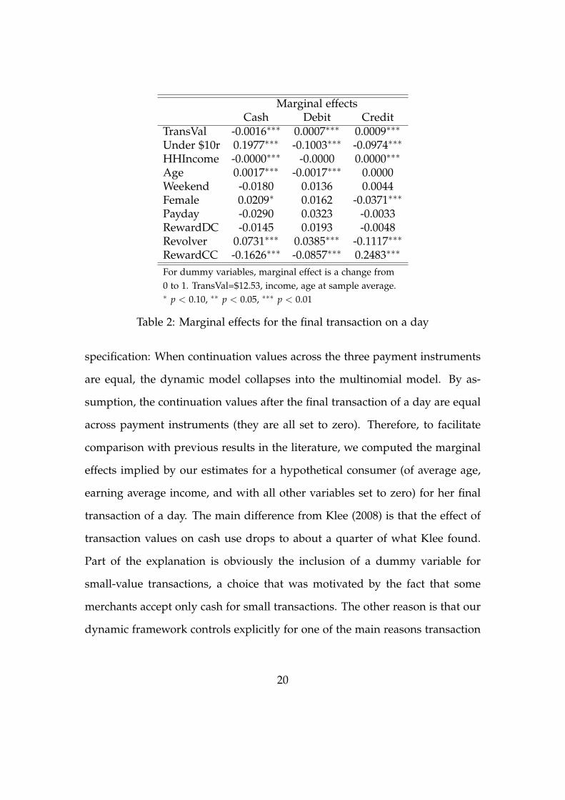
Marginal effectsCash Debit Credit

TransVal -0.0016∗∗∗ 0.0007∗∗∗ 0.0009∗∗∗

Under $10r 0.1977∗∗∗ -0.1003∗∗∗ -0.0974∗∗∗

HHIncome -0.0000∗∗∗ -0.0000 0.0000∗∗∗

Age 0.0017∗∗∗ -0.0017∗∗∗ 0.0000Weekend -0.0180 0.0136 0.0044Female 0.0209∗ 0.0162 -0.0371∗∗∗

Payday -0.0290 0.0323 -0.0033RewardDC -0.0145 0.0193 -0.0048Revolver 0.0731∗∗∗ 0.0385∗∗∗ -0.1117∗∗∗

RewardCC -0.1626∗∗∗ -0.0857∗∗∗ 0.2483∗∗∗

For dummy variables, marginal effect is a change from0 to 1. TransVal=$12.53, income, age at sample average.∗ p < 0.10, ∗∗ p < 0.05, ∗∗∗ p < 0.01

Table 2: Marginal effects for the final transaction on a day

specification: When continuation values across the three payment instruments

are equal, the dynamic model collapses into the multinomial model. By as-

sumption, the continuation values after the final transaction of a day are equal

across payment instruments (they are all set to zero). Therefore, to facilitate

comparison with previous results in the literature, we computed the marginal

effects implied by our estimates for a hypothetical consumer (of average age,

earning average income, and with all other variables set to zero) for her final

transaction of a day. The main difference from Klee (2008) is that the effect of

transaction values on cash use drops to about a quarter of what Klee found.

Part of the explanation is obviously the inclusion of a dummy variable for

small-value transactions, a choice that was motivated by the fact that some

merchants accept only cash for small transactions. The other reason is that our

dynamic framework controls explicitly for one of the main reasons transaction

20

values might matter: the cash-in-advance constraint.

Moreover, the individual-level data show that other factors are just as im-

portant: Revolvers are much less likely to use credit cards than convenience

users. On the other hand, credit card reward programs appear to be highly

effective in steering consumers toward credit card use. Interestingly, debit card

reward programs do not have the same effect.

6.2 Are consumers forward-looking?

Our model and the rest of the literature on payment choice can be thought of

as addressing two extremes: We endow consumers with a great deal of infor-

mation about their future transactions while the rest of the literature thinks

of them as completely myopic. How important is this difference empirically?

The simplest way to answer this question is to compare the choice probabili-

ties of the two models. As noted before, the choice probabilities for the final

transaction coincide with that of a multinomial logit model, but they may differ

if the consumer plans to conduct more transactions.

Table 3 compares the payment instrument choice probabilities for the first

transaction of the day for different total numbers of daily transactions. The

same hypothetical consumer as in the previous subsection is assumed to start

the day with $20, and all daily transactions are assumed to be for $12.53 (the

median transaction value). Table 3 shows that the model predicts rather dif-

ferent choice probabilities in the five scenarios. In particular, the probability

of using cash drops from 40 percent in the case of a single transaction, to just

below 30 percent if she makes only one additional transaction. The drop in

21

Daily Choice probabilities∗

transactions Cash Debit Credit1 0.4070 0.2397 0.35332 0.2947 0.2851 0.42023 0.2289 0.3117 0.45954 0.1827 0.3303 0.48705 0.1484 0.3442 0.5074

∗Dummy variables set to 1, except for “Under$10;”transaction value at sample median (=$12.53); age,income at sample average.

Table 3: Choice probabilities for the first daily transaction for different totalnumbers of transactions

the probability of using cash is monotonic; in the case of a third transaction

it is only roughly half what it would otherwise be. Since our choice model

(like other multinomial logit models) possesses the independence-of-irrelevant-

alternatives property, the relative probabilities of debit and credit do not change.

6.3 Withdrawal costs

Given the estimates of α, αj, β, γ, the model can be used to conduct a cost-

benefit analysis of cash withdrawals. In particular, given α and αj, we compute

the average withdrawal cost by withdrawal methods in our sample:

cj =∑n ∑d αznd + αj

Nj,

where the denominator is the number of observed withdrawals using method

j in the sample. This gives us a measure in units of consumer utility, which

has no natural unit of measurement. To get a sense of the size of withdrawal

22

Relative toMethod ∆EVDC ∆EVD ∆EVC cATMATM 5.57 4.34 2.84 1.00Cashback 7.51 5.85 3.82 1.35Bank teller 6.59 5.13 3.35 1.18Family & friend 6.08 4.74 3.10 1.09Other 6.38 4.97 3.25 1.15

Table 4: Withdrawal costs

costs, we compare them with the expected benefit of having cash, defined as:

∆EV = E[V(pmd

T , 0, T)]− E [V(0, 0, T)] ,

that is, the change in the expected utilities from making a payment of $12.53

for the hypothetical consumer of the previous subsections. In fact, we compute

this difference for debit and credit card holders (∆EVDC), debit card holders

who do not have a credit card (∆EVD), and credit card holders who do not

own a debit card (∆EVC).

Table 4 shows that, depending on the withdrawal method, it takes any-

where from 6 to 8 (median-sized) transactions to recoup the average with-

drawal cost for consumers who have a debit card and a credit card (with no

debt). For those who can only use a debit card instead of cash, withdrawals are

less costly (cash is more useful): it takes them 4 to 6 (median-sized) transactions

to make up for the withdrawal cost. Those with only a credit card recoup these

same costs in 3–4 transactions.

The table also shows that ATM withdrawals are the least expensive, in util-

ity terms, followed by getting cash from family and friends, other sources (in-

cluding employers, check-cashing stores, cash refunds from returning goods,

23

and unspecified locations), bank tellers, and retail store cash back. The differ-

ence between the least expensive and the most expensive source is about 35

percent.

6.4 Withdrawals

The solution to inventory theoretic models of cash demand (Baumol (1952), To-

bin (1956), Alvarez and Lippi (2009)) is an (s, S) policy function, which specifies

a level of cash balances s at which cash holdings are reset to S. As discussed

above, consumers in our model do not optimize the size of their withdrawals,

they withdraw just enough cash to carry them through the day. Therefore,

a straightforward comparison between our model and the inventory theoretic

studies does not exist. We can, however, compute the probability that someone

makes a withdrawal before a particular transaction.

Figure 3 depicts these probabilities for consumers with different payment

instruments in their portfolio. The hypothetical scenario behind the graph is

that a consumer (average income, average age, employed, male) knows that he

will have to make two, $12.50 transactions during the day. The horizontal axis

denotes different amounts of cash in his wallet before the withdrawal opportu-

nity preceding the first transaction, and the vertical axis denotes the probability

that he will make a $25 withdrawal before the first transaction. The different

lines correspond to different bundles of available payment instruments.

The solid line denotes the extreme case, where no credit or debit card is

available to the consumer; therefore, he will have to make a withdrawal before

the first transaction if he has less than $12.50 in his wallet. If he has more than

24

0 5 10 15 20 25 300

0.1

0.2

0.3

0.4

0.5

0.6

0.7

0.8

0.9

1

Cash before withdrawal

Pro

babi

lity

of w

ithdr

awal

Debit and credit (no debt)Debit and credit (revoler)Debit, no creditNo debit, credit (no debt)No debit, credit (revolver)No debit or credit

Figure 3: Withdrawal probabilities with different payment instrument bundles

that, he can afford to wait with the withdrawal until after the first transaction.

Note that withdrawal costs also have a random component, so there is an

option value of waiting. Figure 3 shows that consumers will use this option

half the time. Finally, if he already has $25 or more in his pocket, there is no

reason to get more cash.

The withdrawal decisions follow similar step-functions for every other payment

instrument bundle. What stands out from the graph is that a person who re-

volves credit card debt and has no debit card (shown by squares) also values

cash highly and is very likely to make a withdrawal if he is low on cash (<

$12.50). The option to delay a withdrawal, if he has enough cash (≥$12.50) ap-

pears more valuable than for somebody with no alternative payment instrument,

25

as indicated by the precipitous drop in the withdrawal probability. Since

withdrawals are quite expensive, having just one additional option to complete

a transaction already reduces the need for a withdrawal, especially if the bene-

fits of the withdrawal (an expanded bundle of available payment instruments)

can only be enjoyed in one additional transaction.

A similar line of reasoning explains why a convenience user of credit cards

(shown by circles) will be not very likely to incur the cost of a withdrawal, even

if his or her cash balances are low before the first transaction. Debit card users

without a credit card (shown by stars), are even less likely to make a with-

drawal, suggesting that debit cards are a closer substitutes for cash payments

(at least at lower values) than credit cards are.

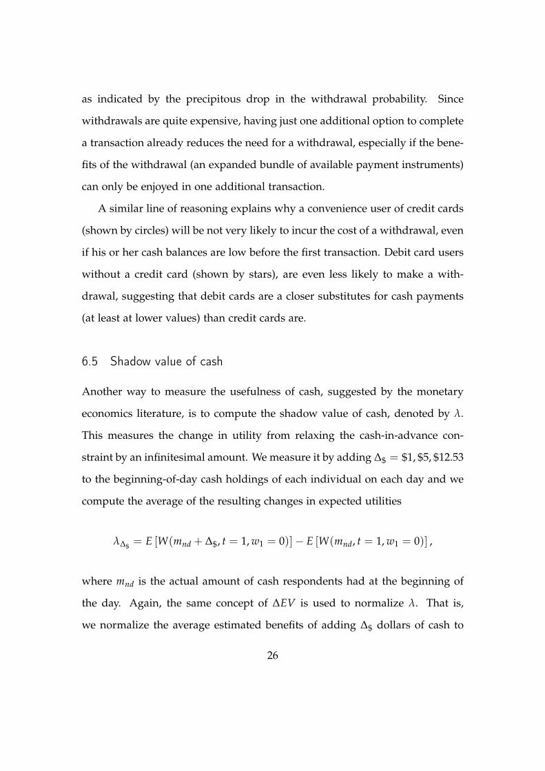
6.5 Shadow value of cash

Another way to measure the usefulness of cash, suggested by the monetary

economics literature, is to compute the shadow value of cash, denoted by λ.

This measures the change in utility from relaxing the cash-in-advance con-

straint by an infinitesimal amount. We measure it by adding ∆$ = $1, $5, $12.53

to the beginning-of-day cash holdings of each individual on each day and we

compute the average of the resulting changes in expected utilities

λ∆$ = E [W(mnd + ∆$, t = 1, w1 = 0)]− E [W(mnd, t = 1, w1 = 0)] ,

where mnd is the actual amount of cash respondents had at the beginning of

the day. Again, the same concept of ∆EV is used to normalize λ. That is,

we normalize the average estimated benefits of adding ∆$ dollars of cash to

26

all consumers’ beginning-of-day payment instrument bundles, by the expected

utility that expanding the payment instrument bundle from {debit, credit} to

{∆$, debit, credit} would give for a single ∆$ transaction.

λ$1

∆EVDC ∼ 0.0164

λ$5

∆EVDC ∼ 0.1117

λ$12.53

∆EVDC ∼ 0.2892.

The costless relaxation of every consumer’s budget constraint by the median

transaction amount ($12.53) yields on average about a quarter of the expected

utility of increasing the payment instrument choice set from debit and credit

to cash, debit, and credit of the hypothetical consumer of subsection 6.3. The

fact that this number is much lower than 1 suggests that a number of people

in our sample are either already able to use cash for all of their transactions

or only make transactions larger than $12.53; so for them the shadow value is

zero. (Of course, doing away with the restriction of zero continuation value at

the end of the day would change this.)

6.6 Simulations

Table 5 displays various moments in our data and shows how well the model

replicates them. We considered several scenarios, the results for all of them

based on 1,000 independent simulations.

First, to get an idea of how well the model explains the data, we ran a

simulation of the model with the estimated parameters. Shocks were drawn

27

Payment instrument choiceCash Debit card Credit card

Data 0.4990 0.2906 0.2104

SimulationDCPC starting cash 0.4657 0.3131 0.2212$0 starting cash 0.2232 0.4567 0.3201

Simulation—No ATMDCPC starting cash 0.4589 0.3180 0.2231$0 starting cash 0.1978 0.4729 0.3293

Simulation—Very Costly WDCPC starting cash 0.4175 0.3492 0.2333$0 starting cash 0.0066 0.6004 0.3930

WithdrawalsNumber Share of methods

ATM Cashback Bank teller Fam. & fr. OtherData 479 0.3549 0.0731 0.1545 0.2338 0.1837

SimulationDCPC starting cash 304 0.4863 0.0155 0.1052 0.2418 0.1513$0 starting cash 824 0.4679 0.0182 0.1121 0.2442 0.1576

Simulation—No ATMDCPC starting cash 246 0 0.0427 0.2172 0.4433 0.2967$0 starting cash 707 0 0.0485 0.2228 0.4314 0.2972

Simulation—Very Costly WDCPC starting cash 2 0.2115 0.1895 0.1905 0.2050 0.2035$0 starting cash 35 0.1989 0.2019 0.1991 0.2010 0.1991

Table 5: Simulation results

28

according to the specified distributions, and the exogenous beginning-of-the-

day cash balances were set to the values observed in the data (“DCPC starting

cash"). Comparing the first two lines of the upper panel of the table shows that

the model does fairly well in capturing the payment instrument choices. While

the share of cash payments is somewhat underpredicted (46.57 percent vs. 49.9

percent in the data) and, correspondingly, debit and are credit overpredicted,

the differences are fairly small.

On the other hand, the model performs much worse with withdrawals, a

result that is not entirely surprising given our simplistic framework. Compar-

ing the first two lines of the bottom panel of Table 5 shows that instead of

the 479 withdrawals in the data, the model is able to predict only 304. We

suspect three reasons for this. First, since the continuation value at the end of

the day is set to zero and most individuals do not make more than two daily

transactions, the high cost of withdrawals becomes prohibitive unless a very

favorable shock is drawn. Second, we assume that agents start the day with an

exogenous stock of cash, for which they do not have to pay. Therefore, many of

them are able to make cash payments without making a withdrawal. Finally,

of the 1,722 individuals in our sample, only 19 report not having a debit or

credit card, meaning that the majority of the households are able to transact

even without cash.

To understand better the role of the beginning-of-the-day cash balances,

we re-ran the simulations with each consumer’s beginning-of-day cash bal-

ances set to zero ("$0 starting cash"). This leads to a considerable drop in

cash payments: 22.32 percent versus 46.57 percent in the previous simulation.

These simulations yield many more cash withdrawals than in the data (824

29

versus 479), but the distribution across withdrawal methods is rather similar

to the "DCPC starting cash" simulation. Both simulations overpredict ATM

withdrawals at the expense of, for the most part, bank teller and cashback.

Since cashbacks work differently in real life than the other methods, they re-

quire a preceeding debit payment and since we have not explicitly modeled

this, it is no surprise that the prediction is off. The bank teller result is more

discouraging.

A potential use of a structural model is to run policy experiments. The

particular experiment we had in mind was to remove the possibility of ATM

withdrawals (technically, we made ATM withdrawals very costly). That is, we

asked what cash use would look like today had ATMs not been invented. The

answer can be found in the "Simulation—No ATM" sections of each panel in

Table 5. Surprisingly, cash use does not change much in either model com-

pared with the respective baseline simulations: Cash use drops by less than a

percentage point in the model with the observed starting cash balances and by

about 2.5 percentage points in the model with $0 starting cash balances. The

number of withdrawals drops by about a sixth in both simulations, and “Fam-

ily and friends” become the primary source of cash. This highlights the partial

equilibrium nature of our model: Where would family members and friends

acquire this much additional cash?

Finally, to verify some of the above conjectures about what could be wrong

with the model, we ran another experiment, where all withdrawal methods

were made very expensive. In this case, the share of cash transactions dropped

to 41.75 percent and 0.66 percent in the two simulations. This result con-

firms that the exogenous starting cash balances drive the results to a very

30

large extent. Interestingly, even with the extremely high withdrawal cost in

these scenarios, withdrawals do not disappear from the economy. The two

withdrawals reported on the penultimate line of the bottom panel of Table 5

show that of the 19 respondents who had no debit or credit card there were

two days when the exogenous starting cash balances were not able to cover the

spending during those days. In these cases respondents are forced to make a

withdrawal, regardless of the costs. Moreover, these 19 respondents recorded

payments on 35 days, so when their beginning-of-day cash balances are set to

$0, they all have to make withdrawals on these days regardless of the with-

drawal costs. The roughly uniform distribution across withdrawal methods

shows that the random component of the cost drives this choice; the known

components are equal(ly high).

All in all, the results of these simulations are mixed. On one hand, the

model yields reasonable predictions for payment instrument choice, which is

encouraging, but the simplistic framework for withdrawals clearly hinders it

from providing a clear link between cash withdrawals and payment instrument

choice. Future work will be directed toward extending the model so that it is

able to explain observed withdrawal amounts, not just frequencies. This will

help relax the assumption of only one withdrawal a day. Perhaps even more

restrictive in the current formulation is that of the zero end-of-day continuation

value. This was originally motivated by computational considerations: evalu-

ating long sequences of transactions is still quite slow. A solution to this can

be introducing a change in the information structure of the model: Not giving

consumers full information about future transaction-specific variables enables

us to recast the finite period model into an infinite horizon model. Solving for

31

the value function in that model is more involved, however.

7 Conclusion

Using a new, transaction-level dataset of consumer payment choice, we are able

to further our understanding of how consumers prefer to settle transactions.

First, payment instrument bundles matter: Whether consumers earn rewards

on their credit cards or pay interest on credit affects their choices markedly.

Second, technology matters: Even in the simple model of this paper, we see

substantial differences in the cost of obtaining cash. Third, payment instrument

choice is ultimately a dynamic decision: Using an instrument for a transaction

may limit its availability for future transactions. While much of monetary eco-

nomics has focused on analyzing the optimal withdrawal policy that helps

agents transact at minimal cost, an alternative margin that consumers can ex-

ploit in liquid asset management is payment instrument choice. As financial

innovation blurs the boundary between transactions and savings accounts, this

margin is likely to become even more important.

Bibliography

Alvarez, Fernando and Francesco Lippi. 2009. “Financial Innovation and the

Transactions Demand for Cash.” Econometrica 77 (2):363–402.

———. 2012. “A Dynamic Cash Management and Payment Choice Model.”

Mimeo, Consumer Finances and Payment Diaries: Theory and Empirics.

32

Bar-Ilan, Avner. 1990. “Overdrafts and the Demand for Money.” American

Economic Review 80 (5):1201–16.

Baumol, William J. 1952. “The Transactions Demand for Cash: An Inventory

Theoretic Approach.” The Quarterly Journal of Economics 66 (4):545–556.

Bounie, David and Yassine Bouhdaoui. 2012. “Modeling the Share of Cash

Payments in the Economy: an Application to France.” International Journal of

Central Banking 8 (4):175–195.

Chiu, Jonathan and Miguel Molico. 2010. “Liquidity, Redistribution, and the

Welfare Cost of Inflation.” Journal of Monetary Economics 57 (4):428–438.

Cohen, Michael and Marc Rysman. 2013. “Payment Choice with Consumer

Panel Data.” Working Paper 13-6, Federal Reserve Bank of Boston.

Eschelbach, Martina and Tobias Schmidt. 2013. “Precautionary Motives in

Short-term Cash Management - Evidence from German POS Transactions.”

Discussion Paper Series 2013,38, Deutsche Bundesbank, Research Centre.

Fung, Ben, Kim Huynh, and Leonard Sabetti. 2012. “The Impact of Retail

Payment Innovations on Cash Usage.” Working Papers 12-14, Bank of

Canada.

Klee, Elizabeth. 2008. “How People Pay: Evidence from Grocery Store Data.”

Journal of Monetary Economics 55 (3):526–541.

Koulayev, Sergei, Marc Rysman, Scott Schuh, and Joanna Stavins. 2012. “Ex-

plaining Adoption and Use of Payment Instruments by U.S. Consumers.”

Working Paper 12-14, Federal Reserve Bank of Boston.

33

Lagos, Ricardo and Randall Wright. 2005. “A Unified Framework for Monetary

Theory and Policy Analysis.” Journal of Political Economy 113 (3):463–484.

Miller, Merton H. and Daniel Orr. 1966. “A Model of the Demand for Money

by Firms.” Quarterly Journal of Economics 80 (3):413–435.

Nosal, Ed and Guillaume Rocheteau. 2011. Money, Payments, and Liquidity. MIT

Press Books. The MIT Press.

Rust, John. 1987. “Optimal Replacement of GMC Bus Engines: An Empirical

Model of Harold Zurcher.” Econometrica 55 (5):999–1033.

Sastry, A. S. Rama. 1970. “The Effect of Credit on Transactions Demand for

Cash.” The Journal of Finance 25 (4):777–781.

Tobin, James. 1956. “The Interest-Elasticity of Transactions Demand For Cash.”

The Review of Economics and Statistics 38 (3):241–247.

Train, Kenneth E. 2009. Discrete Choice Methods with Simulation. Cambridge

Books. Cambridge University Press, 2nd ed.

von Kalckreuth, Ulf, Tobias Schmidt, and Helmut Stix. 2009. “Choosing and

Using Payment Instruments: Evidence from German Microdata.” Working

Paper Series 1144, European Central Bank.

34