Deakin Research Online This is the published version: Ahmed, Salma and Ray, Ranjan 2011, Trade-off between child labour and schooling in Bangladesh: the role of parents' education, Monash University, Melbourne, Vic Available from Deakin Research Online: http://hdl.handle.net/10536/DRO/DU:30054864 Reproduced with the kind permission of the copyright owner. Copyright : 2011, Monash Universit

Trade-off between child labour and schooling in Bangladesh:

The role of parents’ education

Salma Ahmed* and Ranjan Ray

†

Department of Economics

Monash University

Wellington Road

Clayton Campus VIC 3800

Australia

August 2012

Abstract

This paper investigates the effect of child labour on child schooling using the 2002 dataset from the Bangladesh National Child Labour Survey (NCLS). The study provides evidence on the sensitivity of

the results to the methodology adopted and the gender of the child. Working hours have an adverse

effect on the child’s schooling outcome and the result is robust to the procedure used, but the precise

nature of the relationship varies between the parametric and non-parametric approaches. While the former suggests a U-shaped relationship between working hours and child schooling, there is a

monotonic and inverse relationship between the two in case of the latter. The study also provides

evidence that suggests that the gender of the child affects the nature of the relationship, as do the parental characteristics, especially parental education. These results attain special policy significance

in view of the evidence that both parents show a significant preference for educating a female child

that appears to be at odds with the picture of gender bias in favour of the male child in South Asia portrayed in the literature.

JEL Classification: J13; J22; J24; O12

Key words: Child labour, education, Bangladesh

* Corresponding author. Tel.: 61 3 95626169; fax: 990 55476. Email address: Salma.Ahmed@monash.edu

† Tel.: 61 3 99020276; fax: 990 55476. Email address: Ranjan. Ray@monash.edu

2

1. Introduction Much of the literature concerning the effect of child labour on education concludes that educational

attainment is likely to be lower for children who combine work and schooling (Ersado 2005,

Ganglmair 2006, Jensen and Nielsen 1997, Rammohan 2012, Sedlacek et al. 2009).3 Following the

seminal paper by Basu and Van (1998), a number of studies explicitly consider the trade-off between

child labour and schooling (Basu 1999, Basu and Tzannatos 2003, Edmonds 2007, Emerson and

Souza 2003, Udry 2006). Heady (2003), however, derives slightly different results for Ghana and

concludes that child labour does not affect school attendance but substantially interferes with the

quality of schooling with respect to children’s reading and mathematics ability. Other research

focusing on school performance arrive at similar conclusions, including Patrinos and Psacharopoulas

(1995) in Paraguay, Patrinos and Psacharopoulos (1997) in Peru, Parikh and Sadoulet (2005) in

Brazil. By contrast, Ray (2000a), Maitra and Ray (2002) and Ersado (2005) argue that children tend to

combine school and labour without detrimental effects on their school performance, and it might well

be the case that their earnings from work make their schooling possible. Most of these analyses are

based on children’s participation rate rather than hours worked. Exceptions are Akabayashi and

Psacharopoulos (1999), Boozer and Suri (2001), Rossati and Rossi (2003), Ray and Lancaster (2005),

Gunnarsson et al. (2006), Han (2008), Goulart and Bedi (2008), Beegle et al. (2009), Kana et al.

(2010), and Zabaleta (2011). Arguably, child workers who spend longer hours on work activities will

have little time for school attendance and study and this will hamper their educational progress.

Exhaustion from longer hours of work could also prevent children from being attentive inside and

outside the classroom, which has implications for educational performance. Hence, this is an

important issue, and one that should be addressed by policymakers.

A factor that holds promise for improving children’s education and reducing child labour is

parental education. Arguably, if parents care about the human capital attainment of their children,

higher level of parental education should result in more schooling and less child labour, even in poor

households.4 Though there has been much discussion on the role of parents’ education on child labour

and child schooling (see, for example, Coulombe 1998, Deb and Rosati 2002, Ganglmair 2006,

Grootaert 1999, Han 2008, Shafiq 2007), there is a little empirical evidence on their impact on the

trade-off between child labour hours and child schooling.

3 In this paper, we use the terms ‘child labour’ and ‘child work’ interchangeably. 4However, it is often posited that more educated parents in poor households without access to credit may face a

trade-off between education and current consumption; this does not necessarily mean that children of more educated parents are more likely to go to school. Indeed, depending on circumstances, caring parents might

insist on their children working, and use the additional income to improve their children’s nutrition rather than

increasing expenditure on education. However, another possibility is that even during income shocks (for

example, unemployment and natural disasters), a household with educated parents is less likely to pull a child

out of school, or to send a child to work, or both, because educated parents are more likely to have safety nets

(for example, insurance).

3

The principal aim of this paper is to investigate whether the number of working hours

adversely affects schooling outcomes of children in Bangladesh, a low-income country where there is

still significant use of child labour in many parts of the economy. We also explore how parents’

educational levels affect the work-schooling trade-off between genders. As regards Bangladesh, only

a limited number of studies have investigated the trade-off between child labour and schooling (Amin

et al. 2006, Arends-Kuenning and Amin 2004, Ravallion and Wodon 2000, Shafiq 2007). However,

Khanam (2008) finds that children tend to combine schooling with work. Apart from these studies,

there has been a quite different strand of literature, which documents the link between child labour

and household participation in group-based credit programs (Islam and Choe 2011, Ridao-Cano

2001). There is one consistent finding from these papers: household access to credit has not

significantly reduced child labour in Bangladesh. In the case of child schooling, the evidence is

mixed. However, none of these studies investigate whether parental education levels affect the work-

schooling trade-off.

In this paper, we make the following contributions beyond these studies. First, we use an

instrumental variable (IV) estimation strategy because the number of hours that a child works is

endogenously chosen. This is similar to the most recent literature on developing countries (Beegle et

al. 2009, Boozer and Suri 2001, Goulart and Bedi 2008, Gunnarsson et al. 2006) which uses an IV

strategy to identify the effect of child labour. We also use a non-parametric approach for further

investigation of the relationship between child labour hours and schooling. Second, we explore the

selectivity biases that emerge in child labour studies. Hours of work are only available for working

children; children who work different hours might have unobserved characteristics that could be

correlated with the unobservables in the outcome equation (in this case, school), causing our estimates

to be biased and inconsistent. However, this estimation bias has received very little attention in most

studies that estimate the effect of the number of working hours on child schooling outcomes

(Ravallion and Wodon 2000, Ray and Lancaster 2005). Finally, the empirical analysis is carried out

by utilising the Bangladesh National Child Labour Survey data for 2002-2003. This dataset has not

been used in the previous literature to investigate the trade-off between child labour hours and child

schooling in Bangladesh.

We find that the working hours adversely affect child schooling from the very first hour of

work, but the marginal impact of child labour hours weakens when working hours increase. However,

a non-parametric approach suggests that hours worked by children decrease their schooling. We also

find that parents’ education shifts the work-schooling trade-off in favour of education; the mother’s

educational attainment has stronger marginal effects on the work-schooling trade-off than the father’s

education. We note that the mother’s and father’s education (as measured by the highest grade

attained) shows a significant preference for educating a female child. The same incentive effect is not

4

found for a male child, which suggests that male children are more likely to work. Finally, a sample

consisting of only working children introduces a significant bias of IV estimates of the work-

schooling trade-off.

2. Features of child labour in Bangladesh

In spite of legislation, children are relatively less protected in Bangladesh. As regards Bangladesh, a

National Child Labour Survey (henceforth NCLS) conducted in 2002-2003 by the Bangladesh Bureau

of Statistics (BBS), found that approximately 5 million (14%) of the total 35 million children between

the ages of 5 and 14 were economically active. Of this total 3.5 million (71%) were boys and 1.5

million (29%) were girls. Official statistics have shown that the total working population between the

ages of 5 and 17 was approximately 7.9 million, of which 5.8 million (73%) were boys and 3.1

million (27%) were girls (NCLS 2002).

The widespread prevalence of child labour in Bangladesh, despite the government’s programs

and laws prohibiting work by children, suggests that additional policy measures to curb child labour

are warranted. At present, there are 25 special laws and ordinances to protect and improve the status

of children in Bangladesh (Khanam 2006). It is widely believed that there is a lack of harmony among

laws that uniformly prohibit the employment of children or set a minimum age for employment.

Under the current law, the legal minimum age for employment varies, between 12 and 16, depending

on the sector (Khanam 2006). However, Bangladesh Export Processing Zones Authority (BEPZA)

has restricted the minimum age to 14 for employment in EPZs.

In 1995, Bangladesh signed a Memorandum of Understanding (MOU) which had been

undertaken by the ILO and UNICEF to eliminate child labour from the garments industry. As reported

by Rahman et al. (1999), this approach neither reduced child labour among these children nor

increased their schooling. A second MOU was undertaken by the same parties in 2000 to reaffirm the

agreements of the first MOU and to develop a long-term and sustainable response to monitoring child

labour in the garments industry (Khanam 2006). Furthermore, since 1993, primary school education

has become compulsory in Bangladesh, and the country has adopted school subsidy provision to

improve schooling and thereby attract and retain children. However, previous literature has shown

that participation in the child labour force may not be responsive to education-related policy measures

(see, for example, Ravallion and Wodon 2000). Another educational incentive program that

encouraged girls to increase their (junior) secondary schooling (i.e. Grade 6-10) was found to be

effective in increasing secondary school attendance (see Arends-Kuenning and Amin 2004).

However, no research thus far attempts to shed light on whether this particular subsidy reduces

participation in child labour.

5

3. Data and variables

3.1. Data

The empirical analysis of this paper is based upon the individual-level data for 2002-2003 National

Child Labour Survey (henceforth NCLS). This survey has been designed in the context of the

commitments made by the Government of Bangladesh, following the ratification of the ILO Worst

Forms of Child Labour Convention (No. 182) 1999. The NCLS 2002 was designed to provide reliable

estimates of child labour at national, urban and rural levels, as well as by districts. The NCLS

included a child population between the ages of 5 and 17 from 40,000 households. However, NCLS

excluded children living in the streets or in institutions such as prisons, orphanages or welfare centres.

The NCLS considers a child (aged 5-17) to be employed if he or she worked at least one hour

during the reference week (the week preceding the day of the survey). However, the survey does not

consider child participation in domestic work to be labour. To enable our empirical analysis, we focus

on children between the ages of 5 and 17 who worked at least one hour during the reference week as a

paid (wage) employee (paid in cash or in kind), or who was self-employed,5 or who worked as an

unpaid employee (for example, work on the family farm or in family businesses) related to the

household head.6 This is especially important as globally only a relatively small fraction of children

work for wages. Furthermore, we follow the definition of work similar to the NCLS, that is, we

exclude domestic work. For the estimation of child labour, five years may be considered extreme

because this is the cut-off age between infancy and childhood. However, it is not unusual in case of

Bangladesh, particularly in rural areas. On the other hand, although the official enrolment age in

Bangladesh is six years, there are some children who start school at the age of five (and therefore, the

start of the potential trade-off between schooling and child labour). We extend the age limit to 17

years in order to capture a better interaction between child labour and education. According to the

education system in Bangladesh, students at the age of 17 should be at the beginning of higher

secondary school. However, the data suggests that there are some children in the age group of 5-17

who are still in primary school. This is very common, especially in rural areas.

The analysis is performed upon a full sample of 14,062, 5-17 year old children drawn from

the survey’s urban and rural respondents. In this sample, 9,404 (67%) are male children and 4,658

(33%) are female children. Out of this sample, 2,801 males and 1,439 females reside in urban areas,

while 6,603 males and 3,219 females reside in rural areas. 8,900 children are actively participating in

5 A self-employed or own-account worker is officially defined as a person who works for his or her own farm or

non-farm enterprise for profit or family gain. 6 NCLS classified children as sons and daughters if they are the son or daughter of the head of the household or

spouse. The father is called the head of the household if the head is identified as male and the mother is called

the spouse (if listed as the opposite sex), and the mother is called the head if the head is identified as female and

the father is called the spouse (if listed as the opposite sex).

6

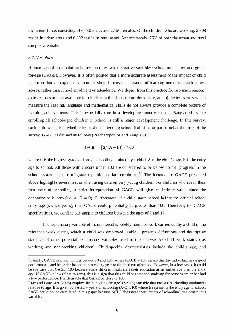
the labour force, consisting of 6,750 males and 2,150 females. Of the children who are working, 2,508

reside in urban areas and 6,392 reside in rural areas. Approximately, 76% of both the urban and rural

samples are male.

3.2. Variables

Human capital accumulation is measured by two alternative variables: school attendance and grade-

for-age (GAGE). However, it is often posited that a more accurate assessment of the impact of child

labour on human capital development should focus on measures of learning outcomes, such as test

scores, rather than school enrolment or attendance. We depart from this practice for two main reasons:

a) test scores are not available for children in the dataset considered here, and b) the test scores which

measure the reading, language and mathematical skills do not always provide a complete picture of

learning achievements. This is especially true in a developing country such as Bangladesh where

enrolling all school-aged children in school is still a major development challenge. In this survey,

each child was asked whether he or she is attending school (full-time or part-time) at the time of the

survey. GAGE is defined as follows (Psacharopoulos and Yang 1991):

GAGE = G/ A − E ∗ 100

where G is the highest grade of formal schooling attained by a child, A is the child’s age, E is the entry

age to school. All those with a score under 100 are considered to be below normal progress in the

school system because of grade repetition or late enrolment.7,8

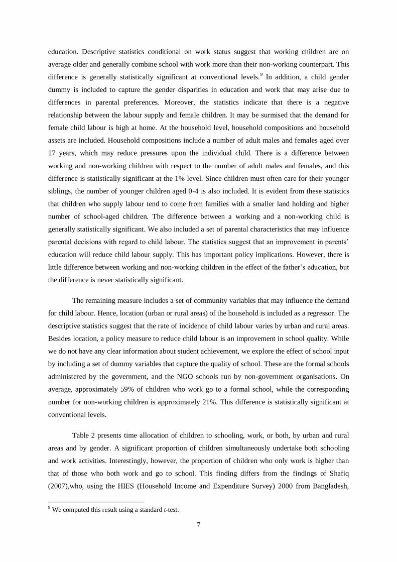
The formula for GAGE presented

above highlights several issues when using data on very young children. For children who are in their

first year of schooling, a strict interpretation of GAGE will give an infinite value since the

denominator is zero (i.e. A–E = 0). Furthermore, if a child starts school before the official school

entry age (i.e. six years), then GAGE could potentially be greater than 100. Therefore, for GAGE

specifications, we confine our sample to children between the ages of 7 and 17.

The explanatory variable of main interest is weekly hours of work carried out by a child in the

reference week during which a child was employed. Table 1 presents definitions and descriptive

statistics of other potential explanatory variables used in the analysis by child work status (i.e.

working and non-working children). Child-specific characteristics include the child’s age, and

7Usually, GAGE is a real number between 0 and 100, where GAGE = 100 means that the individual has a good

performance, and he or she has not repeated any year or dropped out of school. However, in a few cases, it could

be the case that GAGE>100 because some children might start their education at an earlier age than the entry

age. If GAGE is low (close to zero), this is a sign that this child has stopped studying for some years or has had a low performance. It is desirable that GAGE be close to 100. 8Ray and Lancaster (2005) employ the ‘schooling for age’ (SAGE) variable that measures schooling attainment

relative to age. It is given by SAGE = years of schooling/(A-E) x100 where E represents the entry age to school.

SAGE could not be calculated in this paper because NCLS does not report, ‘years of schooling’ as a continuous

variable.

7

education. Descriptive statistics conditional on work status suggest that working children are on

average older and generally combine school with work more than their non-working counterpart. This

difference is generally statistically significant at conventional levels.9 In addition, a child gender

dummy is included to capture the gender disparities in education and work that may arise due to

differences in parental preferences. Moreover, the statistics indicate that there is a negative

relationship between the labour supply and female children. It may be surmised that the demand for

female child labour is high at home. At the household level, household compositions and household

assets are included. Household compositions include a number of adult males and females aged over

17 years, which may reduce pressures upon the individual child. There is a difference between

working and non-working children with respect to the number of adult males and females, and this

difference is statistically significant at the 1% level. Since children must often care for their younger

siblings, the number of younger children aged 0-4 is also included. It is evident from these statistics

that children who supply labour tend to come from families with a smaller land holding and higher

number of school-aged children. The difference between a working and a non-working child is

generally statistically significant. We also included a set of parental characteristics that may influence

parental decisions with regard to child labour. The statistics suggest that an improvement in parents’

education will reduce child labour supply. This has important policy implications. However, there is

little difference between working and non-working children in the effect of the father’s education, but

the difference is never statistically significant.

The remaining measure includes a set of community variables that may influence the demand

for child labour. Hence, location (urban or rural areas) of the household is included as a regressor. The

descriptive statistics suggest that the rate of incidence of child labour varies by urban and rural areas.

Besides location, a policy measure to reduce child labour is an improvement in school quality. While

we do not have any clear information about student achievement, we explore the effect of school input

by including a set of dummy variables that capture the quality of school. These are the formal schools

administered by the government, and the NGO schools run by non-government organisations. On

average, approximately 59% of children who work go to a formal school, while the corresponding

number for non-working children is approximately 21%. This difference is statistically significant at

conventional levels.

Table 2 presents time allocation of children to schooling, work, or both, by urban and rural

areas and by gender. A significant proportion of children simultaneously undertake both schooling

and work activities. Interestingly, however, the proportion of children who only work is higher than

that of those who both work and go to school. This finding differs from the findings of Shafiq

(2007),who, using the HIES (Household Income and Expenditure Survey) 2000 from Bangladesh,

9 We computed this result using a standard t-test.

8

found that children mostly attend school only whereas the proportion of children who both attend

school and also work is relatively small. Rural children are more likely to work and go to school at the

same time than are their urban counterparts. However, urban children are more likely to become idle

(i.e. reportedly involved neither in schooling nor in child labour). The higher proportion of idle

children in urban areas indicates that a household may pull children out of school before completion.

However, the findings about idle children may be under-reported because NCLS 2002 does not

consider domestic work as child labour or because households are hesitant to report child labour

practices to survey collectors. With respect to gender, more female than male children attend school

full-time (i.e. those attend school and avoid child labour), and fewer females than male children are

employed full-time and combine work with schooling.

Table 3 presents the incidence of child labour force participation and school attendance for

children between the ages of 5 and 17. In all areas, the child participation rate in the labour market

increases with age, though not monotonically. Ray (2000a, 2002) also provides similar evidence from

Nepal, Peru and Pakistan. In the case of child schooling, the attendance rate peaks around 12 years in

urban and rural areas, and then falls. The gender picture is similar in both urban and rural areas with

respect to child labour, with males registering a higher participation than females. This finding is

consistent with Ray (2000b), who provides similar evidence from India. However, the situation differs

sharply with respect to child schooling with a more even gender imbalance in the attendance rate

between male and female children in the later age groups of 12-17 years. This observation is also

borne out by Ray (2000a), who finds that Pakistani girls’ schooling falls to nearly half that of boys in

the age groups of 14-17 years. In the context of Bangladesh, there are several possible reasons for this

drop-off. Girls are separated away from male contact at an early age (based on religion). Since there

are few primary schools, and even fewer secondary schools reserved for girls, young females have to

leave school on reaching adolescence. Another possible explanation is that it is customary for girls to

marry early, which tend to further curtail schooling. Additionally, female children are often asked to

do domestic chores, which further discourage educational advancement.

Interestingly, the school attendance rates of rural children in almost all age groups are

consistently larger than their urban counterparts, with the former registering figures approximately

60% for males and 50% for females around 12 years and falls off sharply beyond 14 years. In the case

of urban areas, the attendance rate rarely goes above 50% and falls off sharply beyond 14 years.

Table 4 shows the employment status of children by urban and rural areas and by gender. In

rural areas 52% of working males were unpaid employees and 40% were paid employees. In urban

areas, however, approximately 48% of working males were paid workers and 43% were unpaid

workers (work without pay in family farms or in the family business). Similar patterns are not found

9

for female working children. A large proportion of female child workers worked without pay in

family farms or in the family business, and this is relatively high in rural areas.

These patterns suggest that opportunities for child workers are quite different in rural and

urban areas. In rural areas, children are more likely to engage in agricultural activities and become

unpaid workers, especially female children. In urban areas, children are more likely to find

opportunities for some paid work. The gender difference in employment status among child workers

is also significant in Bangladesh. Young females are more likely than young males to be unpaid

workers in both urban and rural areas. This may imply that male children are increasingly entering the

formal wage labour market rather than working as unpaid workers, and thus allowing female children

to substitute into the unpaid activities.

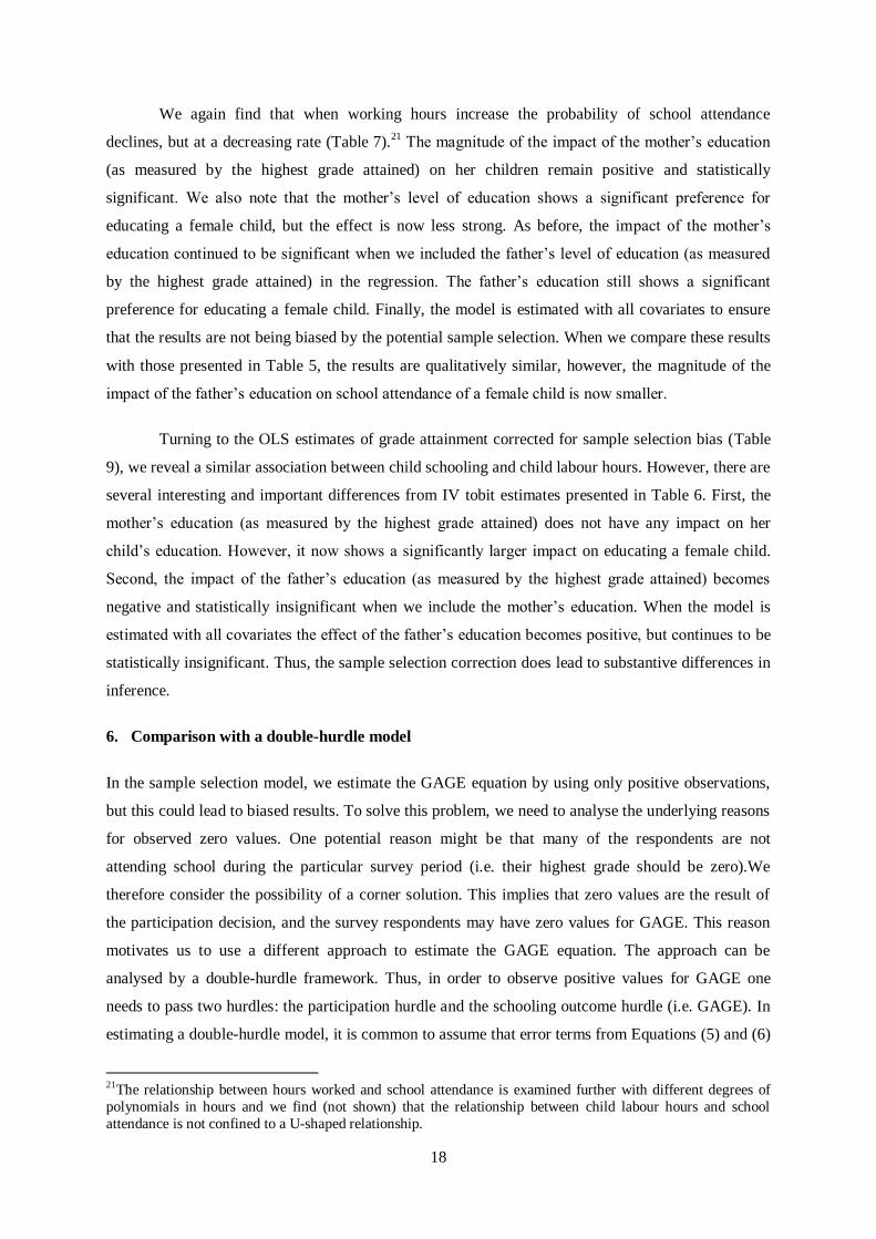
Figure 1 shows that there appears to be a threshold beyond which the number of hours

worked is strongly associated with reduced school attendance in Bangladesh. The number of working

hours appears to have a relatively small impact on school attendance up to the 15-29 hours cohort, but

attendance falls off dramatically when children work more than 29 hours per week. The decline is

more gradual for girls than for boys, perhaps because some kinds of chores and subsistence work are

more compatible with school.

4. Analytical framework and empirical strategy

In this paper, we assume that parental preferences may not be conjugal and that differences may exist

in parental preferences regarding child’s work and schooling. This is consistent with the literature that

suggests that male and female heads of the household may have different utilities, reservation utilities,

and budget constraints and that they therefore may make different decisions (see, for example,

McElroy and Horney 1981). The resolution of the preference difference of the male and female

household heads may depend on the relative bargaining power of each individual, and this power may

depend on (a) control over assets, both current and those brought into marriage; (b) unearned income

or transfer payments and welfare receipts; (c) access to social and interpersonal networks; and (d)

attitudinal attributes. In the absence of direct information on parental preferences, as well as the non-

labour income of each spouse, we shall, in this paper, consider the different role of the mother’s and

father’s education (Basu 2006, Basu and Ray 2001). We propose that women’s education increases

women’s bargaining power in household decisions and if the mother obtains a higher marginal

disutility from child labour than the father, an increase in the bargaining power of a mother will

reduce child labour and increase child schooling.

In this framework, let us assume that a household is comprised of a mother and father and

some number of children. Fertility is assumed to be exogenous. In general, each parent is considered

10

altruistic in that they care about the consumption of each member of the household and the quality

(educational attainment) of their children. All decisions are made by altruistic parents, and children

are treated as recipients of parents’ decisions.10

The parents allocate the child’s total endowment of

time between school attendance and work. Leisure is not included in this analysis for simplification.

Household income must meet the cost of household consumption and schooling. Household income is

generated by a typical household production function with decreasing returns. We assume it is a

function of the parent’s non-labour income, the parent’s labour income and the child’s income. We

shall maintain the strong assumption that non-labour income is exogenous, and we therefore ignore

the fact that current non-labour income probably reflects past labour supply decisions. While primary

education is almost free in Bangladesh, schooling costs can be significant in terms of costs on

transportation, school uniform, utensils and so on, especially for the poor. Parental investment for a

given level of schooling would depend on a vector of child, parental, household and communal

characteristics. Child labour supply equals child’s total endowment of time less school attendance and

depends on a vector of child, parental, household and communal characteristics.

This simplified framework forms the basis of our empirical analysis, which is discussed

below.

Let 𝑆𝑖∗ denote the latent variable that describes household decisions to enrol a child 𝑖 in

school. The equation for 𝑆𝑖∗is written as follows:

𝑆𝑖∗ = 𝛼0 + 𝛼1𝐿𝑖 + 𝛼2𝐿𝑖

2 + 𝛼3𝐺𝑖 + 𝛼4𝐸𝑚 + 𝛼5 𝐺𝑖 ∗ 𝐸𝑚 + 𝛼6𝐸𝑓 + 𝛼7 𝐺𝑖 ∗ 𝐸𝑓 + 𝛼8𝑍 + 𝜇𝑖 (1)

where 𝐿𝑖 represents a child 𝑖’s 𝑖 = 1, . . . . , K weekly working hours in the reference week and its

quadratic term 𝐿𝑖2 captures the non-linear effects of hours worked,

11 𝐺𝑖 is the dummy for a female

child. 𝐸𝑚 and 𝐸𝑓 denote the mother’s and father’s education measured by the highest grade attained.12

Emerson and Souza (2007) conclude that the mother’s and father’s education may affect investments

in the male and female children differently. The gender of the sampled child is, therefore, interacted

with each parent’s education 𝐸𝑗 (𝑗 = mother or father). 𝑍 is a vector of exogenous child, household

and community characteristics that determine 𝑆𝑖∗and 𝜇𝑖 is the random factor.

In practice, however, we do not observe 𝑆𝑖∗. For school attendance, one could observe the

following binary measures:

10 In line with the literature, it is assumed that children do not bargain with their parents because they do not

have a valid fallback option (Bhalotra 2007). 11 Ray and Lancaster (2005) and Han (2008) also employed the quadratic term of the number of working hours

in their study of child labour and schooling. 12Ravallion and Wodon’s (2000) study on child labour and child schooling in Bangladesh also used binary

variables to indicate level of education completed by the mother and the father.

11

𝑆𝑖 = 1 𝑖𝑓 𝑆𝑖

∗ > 0

0 𝑖𝑓 𝑆𝑖∗ = 0

Alternatively, for GAGE:

𝑆𝑖 = GAGE 𝑖𝑓 𝑆𝑖

∗ > 0

0 𝑖𝑓 𝑆𝑖∗ = 0

Thus, the estimating equation is:

𝑆𝑖 = 𝛼0 + 𝛼1𝐿𝑖 + 𝛼2𝐿𝑖2 + 𝛼3𝐺𝑖 + 𝛼4𝐸𝑚 + 𝛼5 𝐺𝑖 ∗ 𝐸𝑚 + 𝛼6𝐸𝑓 + 𝛼7 𝐺𝑖 ∗ 𝐸𝑓 + 𝛼8𝑍 + 𝜇𝑖 (2)

While we estimate Equation (2) by probit if the variable of interest is school attendance, we

use the tobit model if the variable of interest is GAGE because GAGE has observed zero values for

approximately 46% of children aged 7-17.

One potential concern of estimating Equation (2) is that child labour hours and child labour

hours (squared) may not be exogenous. Specifically, certain unobserved factors that determine school

attainment may also explain hours worked, causing our probit or tobit model estimates to be biased

and inconsistent.13

To avoid this endogeneity problem, we use a two-stage instrumental variable (IV)

strategy. There is, however, one other problem. Note that household income included in variable 𝑍 is

most likely to be endogenous because whether or not children work is likely to influence parents’

reservation wages and their labour market participation (Wahba 2006). To avoid endogeneity of this

variable, we include an occupation status of the father to proxy wealth.14

Thus, the reduced-form work equation is written as follows:

𝐿𝑖 = 𝛽0+𝛽1𝐺𝑖 + 𝛽2𝑍 + +𝛽3𝑉𝑖+𝛽4𝐸𝑚 + 𝛽5(𝐺𝑖 ∗ 𝐸𝑚 ) + 𝛽6𝐸𝑓 + 𝛽7(𝐺𝑖 ∗ 𝐸𝑓) + 𝜈𝑖 (3)

where 𝑉𝑖 is the instrumental variable and 𝜈𝑖 is the random factor. Instruments are described and

justified in the following section.

The instrumental variable (IV) procedure can be described as follows. In the first stage, we

estimate Equation (3) by ordinary least squares (OLS) and obtain the residual (𝜐). We follow the same

procedure when the child labour hour (squared) is the dependent variable. In the second stage, we

include predicted residuals from first-stage regressions into Equation (2) as additional regressors. The

13The unobserved determinants could be person-specific or individual attributes, such as ‘motivation’ or

‘energy’ that might drive certain children to both work more and study more. 14We assume that the contribution of children’s income to overall household income is not large. In doing so, we

have abstracted from another significant endogeneity problem.

12

significant coefficients on residuals imply that the null hypothesis of exogeneity of child labour hours

is rejected. Equation (2) can now be written as follows:

𝑆𝑖 = 𝛼0 + 𝛼1𝐿𝑖 + 𝛼2𝐿𝑖2 + 𝛼3𝜐 𝐿𝑖

+ 𝛼4𝜐 𝐿𝑖2 + 𝛼5𝐺𝑖+𝛼6𝐸𝑚 + 𝛼7(𝐺𝑖 ∗ 𝐸𝑚 ) + 𝛼8𝐸𝑓 + 𝛼9(𝐺𝑖 ∗ 𝐸𝑓) +

𝛼10𝑍+𝜇𝑖 (4)

where 𝜐 𝐿𝑖 and 𝜐 𝐿𝑖

2 are predicted residuals from the OLS estimates of child labour hours and child

labour hours (squared) equations, respectively.

4. Results and discussion

The potential endogeneity of the number of working hours is verified through a Hausman test. The

chi-square test rejects the joint exogeneity of hours worked and its square term in almost all

specifications that we estimated (see Tables 5 and 6, bottom). To solve the endogeneity problem, we

relied on instruments such as a set of industry dummies (agriculture, manufacturing, wholesale and

retail and service) where the child works. We choose a sector of employment because the amount of

hours worked that is available for a child depends on the job to which he or she is assigned in a

particular sector. There is no evidence that the industry dummies considered in this paper have any

direct impact on schooling. We assume that the only influence that the sector of employment has on

schooling must come through its effect on the number of hours worked, and not through any other

channels. According to NCLS 2002, children employed in manufacturing and wholesale and retail

work approximately 50 hours or more per week compared to other sectors in Bangladesh. In these

sectors, children may be offered to work more hours, or they may decide to work long hours due to a

higher likelihood of extra payment. For example, it is well known that in the garments industries in

Bangladesh children are offered to work more than the minimum number of hours available (i.e. eight

hours a day), which might partly explain why child labour hours and schooling are not compatible. In

the case of the agriculture or service sectors, it can be assumed that only a small amount of flexibility

in working hours is available. The harvest season, for example, is unlikely to be compatible with

public school schedules. Thus, it is reasonable to assume that jobs in these sectors do not provide time

that can be used for studying.

The exogeneity of these instruments is also checked by empirical tests. The relevant test lends

strong credence to our use of industry dummies as instruments for both ‘child labour hours’ and ‘child

labour hours (squared)’ equations (with a p-value of 0.000) (see Tables A1 and A2 in the Appendix,

bottom).15

Over-identification tests are also conducted to evaluate whether the proposed instruments

15 We perform an 𝐹-test that the coefficients on the industry dummies are jointly zero. The F-statistics ranging

from 137 to 274 depending on different specifications for school attendance, indicating that the instruments add

13

can sensibly be excluded from both ‘school attendance’ and GAGE equations. The Hansen J-statistic

concludes that all instruments can legitimately be excluded in the estimation of both ‘school

attendance’ and GAGE equations (Tables 5 and 6, bottom).

4.1. School attendance

Table 5 presents the results of school attendance using an IV probit for all children. For ease of

interpretation the results are presented as marginal effects. Initially, we include individual covariates,

such as the child’s age, its square term and the dummy variable for a female child, but exclude

education levels of the mother and the father and other covariates as explanatory variables in the

regression (Column 1). We find that there is a significant age effect: age is positive and statistically

significant. This implies that the probability of school attendance increases with the age of the child.

The square of the age of the child shows that there is a non-linearity in the age effect (the square of

the age term becomes negative and statistically significant). As the child gets older, the likelihood that

he or she will drop out of school (due to fail to continue education) and engage in market-oriented

work increases. This is consistent with findings for various countries reported in the literature; see the

review of Dar et al. (2002). Being female reduces the chance of being in school. This is a common

scenario in Bangladesh and in other South Asian countries (Ray 2000a, Rosati and Rossi 2003) where

there is a significant gender differential in the probability of school attendance and this bias is

generally in favour of male children. The marginal effects show that being a female child is associated

with a decrease of approximately 18 percentage points in the probability of school attendance.

The coefficient estimates for ‘child labour hours’ and ‘child labour hours (squared)’ are

statistically significant, but are of opposite signs at conventional levels. The negative magnitude of the

estimated coefficients of the ‘child labour hours’ variable support the proposition that working hours

adversely affects the probability of the child attending school from the very first hour of work.

However, the estimated positive coefficients of ‘child labour hours (squared)’ suggest that the adverse

marginal impact of child labour hours on the schooling variable weakens when working hours

increase.16

significantly to the prediction of the working hours (see Table A1, bottom). The corresponding F-statistics for

GAGE specifications varied between 136 and 272 (see Table A2, bottom). Tables A1 and A2 also report the

adjusted R-squared for school attendance and GAGE regressions, which varied between 0.20 and 0.30. 16 What this implies is that hours worked by a child has a U-shaped relationship with schooling outcomes. The

result is consistent with the findings of Ray and Lancaster (2005). We do not have sufficient evidence to explain

the reasons for this pattern of relationship between child labour hours and school attendance. However, it is

undeniable that long working hours, beyond a certain threshold level, have a negative effect on children’s

education. To explore this issue, we include the third and fourth degrees of polynomials in hours and find that the relationship between child labour hours and the likelihood of school attendance is not always confined to a

U-shaped relationship.

14

Next we turn to an analysis of how parents’ education influences the nature of trade-off

between working hours and school attendance (Column 2). The mother’s level of education (as

measured by the highest grade attained) shows a greater positive effect on the schooling of male and

female children but has a differentially higher effect on the female child, as shown by the positive

coefficient for the interaction of the female dummy with the mother’s level of education. Shafiq

(2007), using the HIES 2000, found similar results for Bangladesh. This result further corroborates the

findings that children’s school attainment is linked to the educational attainment of the parent of the

same sex as the child (see, for example, Emerson and Souza 2007).

Next we include the father’s level of education (as measured by the highest grade attained) to

account for the trade-off between child labour and schooling in the effect of both the mother’s and

father’s level of education (Column 3). Altogether, the results suggest that the father’s education has a

greater positive impact on his daughter’s school attendance than on a son’s. This is indicated by the

interaction of the female dummy with the father’s education and, hence, shifts the trade-off towards a

daughter’s schooling. This is not a new result in the context of Bangladesh. Using the HIES 2000

Shafiq (2007) finds that a female child has a seven percentage point higher probability of being

enrolled in school by having an educated father. One possible explanation is that father’s education

may be more important because fathers are often more educated than mothers in developing countries.

Alternatively, it may be that fathers play a more active role in certain kinds of decisions. On the other

hand, though the effect of the mother’s level of education increases the probability of school

attendance for all children; the preference for educating a female child virtually disappeared when

controlled with the father’s education. We verify the robustness of these results by including

additional covariates, namely household compositions, household assets and community

characteristics (Column 4). The results are summarised as follows: as far the as the effect of child

labour hours is concerned, we find a similar association between the number of hours worked and the

probability of school attendance. The coefficient for a female child is lower but still significant. We

note that the presence of school children between the ages of 5 and 17 reduces the probability of

school attendance. This finding corroborates past evidence from Bangladesh (Amin et al. 2006).

These findings may shed light in favour of the quality-quantity trade-off and the effects of sibling

competition. Furthermore, it is argued that large numbers of school-aged children demand more

resources to be put into their education, which in turn forces them to be employed in case of parental

resource constraints, to make schooling possible for themselves and for their siblings. This may have

a negative impact on their schooling outcome. On the other hand, there is strong evidence that the

presence of adult female members in the household increases the probability of child school

attendance. This effect might reflect the large decision-making power of females among adults in the

household. As expected, the probability of child school attendance increases in urban areas than in

rural areas. We also note that the father’s occupation reduces the probability of attending school if the

15

father is involved in agricultural activities (the reference category is non-agricultural activities). There

are three possible routes whereby a father’s agricultural activities may affect his child’s schooling.

First, a person working in the agricultural sector may be resource constrained compared to those

involved in non-agricultural activities and may decide that it is not worthwhile to send his children to

school at all. Second, agricultural activities in Bangladesh are characterised by seasonal variation, and

therefore, it is not uncommon for families to engage in non-agricultural activities to supplement

household income. Involvement in non-agricultural activities by adult members increases the demand

for child labour in activities where child and adult labour are substitutes. Third, a household whose

primary livelihood is from agricultural activities may see a lack of relevance in formal education.

With respect to parents’ education, we find that both the mother’s and father’s education has a

positive effect on the probability of attending school, though none is statistically significant, possibly

picking up the wealth effect within the household. The positive and significant coefficient of

interaction term between the child’s gender and the father’s education might suggest the trade-off

towards a daughter’s schooling. These results perhaps suggest that parents’ education, particularly the

father’s education, may not be a good proxy for the permanent income effect and, hence, increases the

likelihood that a male child will work.

4.2. GAGE

Further evidence on the adverse impact of working hours on child schooling is shown in Table 6,

which presents marginal effects of IV tobit estimates of GAGE (Columns 1-3). These findings are

supported by Ray and Lancaster (2005) who find similar results measured by SAGE. As expected,

being a female child is associated with a lower grade attainment.

We notice that the mother’s level of education (as measured by the highest grade attained)

shows a positive and significant effect on the grade attainment of her children (Column 2). In

addition, this effect is stronger for educating a female child. Interestingly, the inclusion of the father’s

level of education in the model shows that there is no significant change on the coefficients for the

mother’s level of education, though the magnitude of the coefficient is now smaller (Column 3).17

Also, the magnitude of the impact of the father’s level of education is significantly smaller than that

of the mother’s. The father’s education, however, does not reveal any bias towards a female child.

The final robustness check includes all covariates (Column 4). We again find that being a

female child is associated with lower grade attainments, but this is no longer statistically significant.

This perhaps suggests that grade attainments for female children are determined more by institutional

factors or other issues than by household decisions. Another point is noteworthy. The coefficients for

17 However, these findings must be treated with some caution due to the effect of the ability bias or the effect of

assortative mating on the intergenerational transmission of schooling.

16

child labour hours suggests that the importance of working hours for grade attainment is much

weaker, even after controlling for individual, parental and household characteristics. These results

imply that other factors are more crucial in determining a child’s grade attainment. The results

regarding parents’ education remain in most cases.

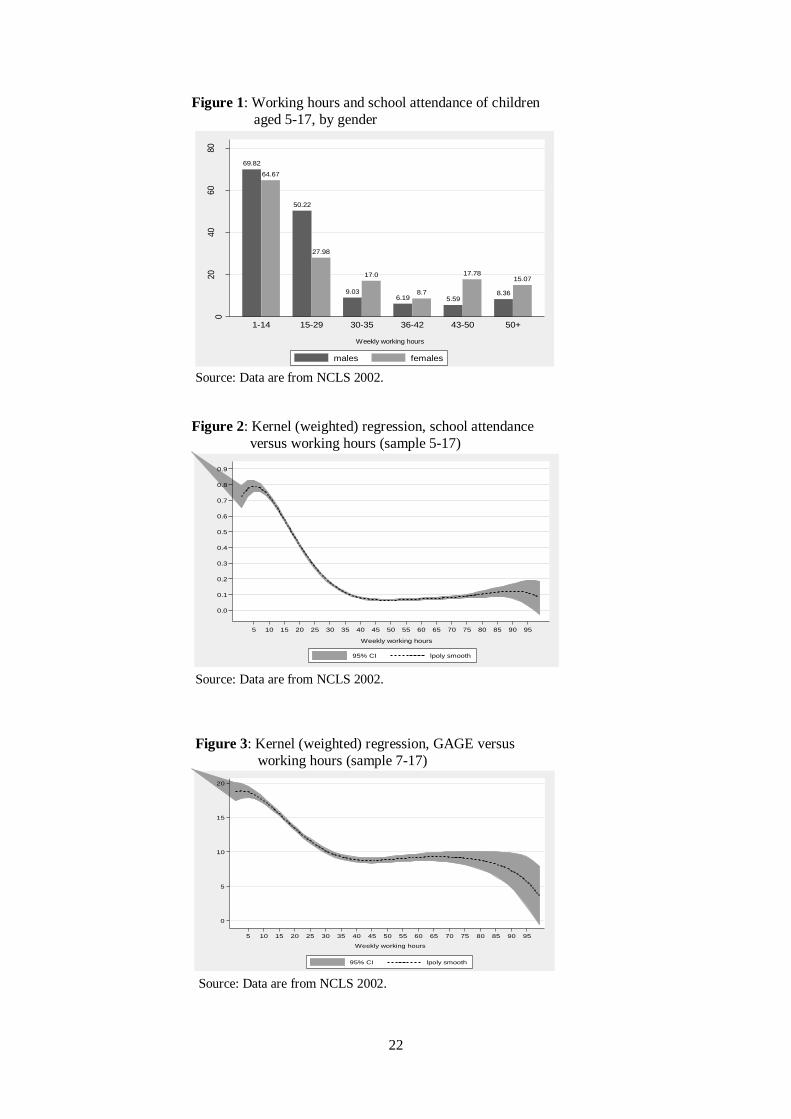
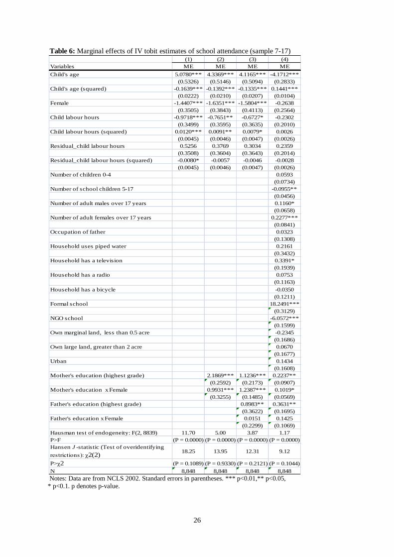
4.3. Results from a non-parametric approach

To make our findings more robust, we further examine the relationship between child labour hours

and schooling with the kernel (weighted) regression approach. The relationship between working

hours and the probability of school attendance is presented in Figure 2. Figure 3 reports the case of

GAGE. A closer examination of Figure 2 shows that the probability of attending school declines

continually with the increase of hours spent at work in economic activities and, hence, provides

evidence that work and schooling are competing activities. This finding is consistent with Guarcello et

al. (2006) who find a similar association in four countries (Bolivia, Mali, Cambodia and Senegal)

between hours worked (spent in domestic chores and economic activity) and not attending school.

Similarly, we find that grade attainment declines if working hours increase (Figure 3).

5. Controlling for sample selection bias

As our estimates refer only to the subsample of children working in economic activity, this could

generate a selection bias in the estimates. Children who participate may have unobserved

characteristics that are correlated with the unobservables in the outcome equation (in this case,

school).18

We address this selection bias by using the sample selection model. The selection (first-

stage regression) should be on hours worked, as children working different hours might share

different characteristics. The selection equation should then be based on a tobit model. However, the

selection variable would be either 0 for non-workers and positive for the other observations. One

simple way to estimate the model is to reformulate the tobit model as a probit model, selecting on a

variable defined as 1 for working children and 0 for non-working children. This is the approach

followed in this paper.19

Hence, the selection equation is:

𝐼𝑖 = 1 𝑖𝑓 𝐿𝑖 = 𝛽𝑥𝑖 + 𝜈𝑖 > 0 0 𝑜𝑡ℎ𝑒𝑟𝑤𝑖𝑠𝑒

(5)

where 𝐼𝑖 and 𝐿𝑖 are the latent and observed working hours of child 𝑖 𝑖 = 1, . . . . , K , respectively. We

observe child work participation as 𝐼𝑖 = 1 if 𝐿𝑖 = 𝛽𝑥𝑖 + 𝜈𝑖 > 0. The vector 𝑥𝑖 denotes the aggregate

18 Working children, for example, who are in school are often found to have lower test scores than non-working

children. However, it may be wrong to say that working leads to poor test outcomes, based simply on that

information. It may be that children with less scholastic aptitude ‘select’ into the state of working, while more

intellectually capable children remain in school. 19Theoretically, this approach may sacrifice some efficiency by discarding information on the dependent

variable. However, this is not necessarily true in a finite sample (Green 1997).

17

form of all the explanatory variables (except for the number of adult males and females over 17 years)

included in Equation (3) and 𝜈𝑖~𝐼𝐼𝐷𝑁 0,1 . The selection correction term or the inverse Mill’s ratio

𝜆 obtained from Equation (5) is included in Equation (6):

𝑆𝑖 = 𝛼0 + 𝛼1𝐿𝑖 + 𝛼2𝐿𝑖2 + 𝛼3𝜐 𝐿𝑖

+ 𝛼4𝜐 𝐿𝑖2 + 𝛼5𝐺𝑖+𝛼6𝐸𝑚 + 𝛼7(𝐺𝑖 ∗ 𝐸𝑚 ) + 𝛼8𝐸𝑓 + 𝛼9(𝐺𝑖 ∗ 𝐸𝑓) +

𝛼10𝑍+𝛼11𝜆𝑖+𝜇𝑖 (6)

In fact, Equation (6) is equivalent to Equation (4), except for the addition of a selection correction

term, which is included to adjust for the non-random sample. Equation (6) is estimated by probit if the

variable of interest is school attendance. This technique is known as the Heckman probit model where

both the selection equation and the outcome equation are binary choices (Van de Ven and Van Praag

1981). In the case of GAGE, Equation (6) cannot be estimated by tobit in a sample selection

framework. In general, the Heckman model assumes that the errors of the participation and schooling

outcomes equations are correlated and the participation decision dominates the schooling outcomes.

Dominance implies that observed zero values for GAGE are the result of participation decision only

and that once the first hurdle (i.e. participation) is passed, censoring is no longer relevant. This

implies that only individuals with positive values for GAGE are included in the GAGE equation. This

is typical of Heckman’s generalised sample selection model (Jones 1989). In our case, we simplify the

Heckman sample selection model by assuming that the participation and schooling outcomes

equations are independent. In this case, the model reduces a probit for participation (Equation 5) and

OLS (Equation 6) using the subsample when GAGE is greater than zero.20

In this case, both equations

are estimated separately.

As is well known, the sample selection model requires an exclusion restriction, in the form of

one or more variables that appear in the participation equation but not in the schooling outcomes’

equation. We include the sex of the household head and the number of adults aged over 17 years in

the household as the exclusion restrictions.

5.1. How important is the selection effect?

The results from the second stage of a selection model of school attendance and GAGE are shown in

Tables 7 and 9. Table 8 presents the probit regression (the selection equation) for the sample of

children aged 7-17. The signs of the estimated coefficient on the inverse Mill’s ratio are of interest

here. The results suggest that the exclusion of the non-working children generates the selection bias.

This is confirmed by a likelihood ratio (LR) test of ρ in four out of five school attendance equations

(see Table 7, bottom).

20A similar method has been used by Aristei et al. (2008) in the study of alcohol consumption.

18

We again find that when working hours increase the probability of school attendance

declines, but at a decreasing rate (Table 7).21

The magnitude of the impact of the mother’s education

(as measured by the highest grade attained) on her children remain positive and statistically

significant. We also note that the mother’s level of education shows a significant preference for

educating a female child, but the effect is now less strong. As before, the impact of the mother’s

education continued to be significant when we included the father’s level of education (as measured

by the highest grade attained) in the regression. The father’s education still shows a significant

preference for educating a female child. Finally, the model is estimated with all covariates to ensure

that the results are not being biased by the potential sample selection. When we compare these results

with those presented in Table 5, the results are qualitatively similar, however, the magnitude of the

impact of the father’s education on school attendance of a female child is now smaller.

Turning to the OLS estimates of grade attainment corrected for sample selection bias (Table

9), we reveal a similar association between child schooling and child labour hours. However, there are

several interesting and important differences from IV tobit estimates presented in Table 6. First, the

mother’s education (as measured by the highest grade attained) does not have any impact on her

child’s education. However, it now shows a significantly larger impact on educating a female child.

Second, the impact of the father’s education (as measured by the highest grade attained) becomes

negative and statistically insignificant when we include the mother’s education. When the model is

estimated with all covariates the effect of the father’s education becomes positive, but continues to be

statistically insignificant. Thus, the sample selection correction does lead to substantive differences in

inference.

6. Comparison with a double-hurdle model

In the sample selection model, we estimate the GAGE equation by using only positive observations,

but this could lead to biased results. To solve this problem, we need to analyse the underlying reasons

for observed zero values. One potential reason might be that many of the respondents are not

attending school during the particular survey period (i.e. their highest grade should be zero).We

therefore consider the possibility of a corner solution. This implies that zero values are the result of

the participation decision, and the survey respondents may have zero values for GAGE. This reason

motivates us to use a different approach to estimate the GAGE equation. The approach can be

analysed by a double-hurdle framework. Thus, in order to observe positive values for GAGE one

needs to pass two hurdles: the participation hurdle and the schooling outcome hurdle (i.e. GAGE). In

estimating a double-hurdle model, it is common to assume that error terms from Equations (5) and (6)

21The relationship between hours worked and school attendance is examined further with different degrees of

polynomials in hours and we find (not shown) that the relationship between child labour hours and school

attendance is not confined to a U-shaped relationship.

19

are independent (Cragg 1971). The model is essentially then a two-step procedure with a probit for

probability of participation in the first stage and a truncated normal regression in the second stage. In

contrast to the sample selection model, a double-hurdle model does not require exclusion restrictions.

However, a specification issue in double-hurdle models concerns the choice of the regressors to be

included in the participation and schooling outcome equations. Indeed, Aristei et al. (2008) argued

that the inclusion of the same set of regressors in each hurdle model makes it difficult to identify the

parameters of the model correctly, and exclusion restrictions must be imposed. The exclusion

restrictions are the same as those used in the sample selection model.

Generally, we identify substantive differences in the results between the sample selection

model and a double-hurdle model, as presented in Table 9. First, the relationship between working

hours and grade attainment is much weaker (the coefficients for working hours are not significant at

conventional levels) (see Columns 4, 6 and 8). Second, the effect of the mother’s education (as

measured by the highest grade attained) becomes insignificant when controlled with the father’s

education (as measured by the highest grade attained); whereas the father’s education now shows a

positive effect on his child’s grade attainment but continues to be statistically insignificant (Column

6). However, the effect of the father’s education now becomes statistically significant after controlling

for individual, household and communal characteristics (Column 8).

7. Additional robustness checks

7.1. Isolating wage employees

In this sub-section, we examine what happens if we restrict ourselves to the sample of wage (paid)

workers. Paid work involves longer hours than other sorts of work, and virtually rules out school

attendance. In contrast, other forms of child labour may be more compatible with schooling. We find

that working hours significantly reduces school attendance but at a decreasing rate (Table 10). On the

other hand, a different pattern emerges with the tobit regressions for GAGE with the number of hours

worked, as we now obtain a statistically insignificant effect of working hours on a child’s grade

attainment (Table 11). When we look at the results for parental characteristics, we find that the effect

of the mother’s education (as measured by the highest grade attained) continues to be significant with

and without controlling for the father’s education (as measured by the highest grade attained) in both

school attendance and GAGE regressions. While the effect of the father’s education is significant in

GAGE equations, it becomes statistically insignificant in school attendance equations if we take into

account the mother’s education. Interestingly, the mother’s education does not show any preference

for educating a female child in all specifications under consideration. While the father’s education

though shows a strong preference for educating a female child in the school attendance equation, this

20

effect virtually disappears when controlled only with the mother’s education and with all covariates in

GAGE equations (see Columns 3 and 4 of Table 11).

7.2. Results by urban and rural areas

There are several points to be noted when looking at urban and rural areas separately (Tables 12 to

15). Looking first at the results for school attendance (Tables 12 and 13), we find that when working

hours increase children are less likely to attend school, but at a decreasing rate in both areas. Results

are reversed with the GAGE specifications (Tables 14 and 15), as the adverse effect of working hours

on grade attainment is, to some extent, significant only among the rural subsample (see Table 15).

This may be due to the pattern of activities available to rural children. Turning next to parents’

education, we reveal that both the mother’s and father’s education (as measured by the highest grade

attained) show a positive and significant effect on school attendance and the grade attainment of male

and female children in rural areas (Tables 13 and 15). The effect of parents’ education, however, is

weaker for school attendance specifications after controlling for individual, household and communal

characteristics (see Column 4 of Table 13). A similar effect of parents’ education is not found in

urban areas. This is especially the case for child’s school attendance. It is important to note that the

mother’s education does not show any bias towards a female child’s school attendance in both urban

and rural areas (see Tables 12 and 13) and in the case of the grade attainment, particularly in urban

areas (Table 14), while for the father’s education, this is true for school attendance in rural areas

(Table 13) and for the grade attainment in both urban and rural areas (Tables 14 and 15).

8. Concluding remarks

This paper has investigated the trade-off between child labour hours and child schooling outcomes in

Bangladesh using the individual-level unit record data from NCLS 2002. We find that working hours

significantly reduces child schooling. Additionally, a non-parametric analysis shows that the

relationship between working hours and schooling is not always confined to a U-shaped relationship

rather there is a monotonic and inverse relationship between the two.

We also find that parental characteristics, especially their level of education, affect the work-

schooling trade-off across genders. The mother’s education (as measured by the highest grade

attained) shows a significant preference in investing in female child’s education. A similar impact is

found for age-adjusted grade attainment. However, the effect of the mother’s education virtually

disappears after controlling for all covariates. This is especially the case for a child’s school

attendance. We find that the father’s education (as measured by the highest grade attained) affects

daughter’s school attendance relative to sons, even after controlling for the mother’s education. The

interpretation of the results is unchanged when the model is estimated with the full set of covariates.

The magnitude of the impact of the father’s education is larger in age-adjusted grade attainment and

21

does not show any significant preference for educating a female child with and without the full set of

covariates. After correcting for potential sources of selection bias, the qualitative results remain for

school attendance but moderately change for age-adjusted grade attainment equations.

These results are in most cases very similar when we restrict our analysis to wage employees

among children or split the sample by urban and rural areas. The most relevant issue is that the trade-

off between working hours and child schooling observed previously still holds, except for tobit

regressions for GAGE. This is especially the case for wage employees among children and when we

use the sample of urban child workers aged between 7-17 years.

These results have strong policy implications. While we find that the mother’s and father’s

education has a positive impact on schooling of their children, the marginal impact of the mother’s

education on a child’s schooling is considerably larger, irrespective of gender of a child. These

findings, therefore, are consistent with our previous proposition that improvement in women’s

schooling and consequent increases in bargaining power have a greater beneficial impact on children

compared with increases in men’s schooling. Therefore, policies which improve education levels,

especially the education levels of women, are more likely to reduce poverty and the incidence of child

labour.

One other result is worth noting for its policy implication. Parent’s educational levels are

more likely to be correlated with the probability that a male child will work rather than go to school.

Although the Bangladesh government adopts a variety of initiatives to ease the problem of child

labour, our results strongly suggest that there is a limited relevance of these policies to supplement

household income, which ultimately results in a higher incidence of child labour, particularly among

young males. While education-related policy measures appear to be ineffective in the context of

Bangladesh, we suggest the need for a combination of policies, such as stronger enforcement of

compulsory schooling for children and an employment generation scheme for adults, to reduce child

labour.

22

Figure 1: Working hours and school attendance of children

aged 5-17, by gender

Source: Data are from NCLS 2002.

Figure 2: Kernel (weighted) regression, school attendance

versus working hours (sample 5-17)

Source: Data are from NCLS 2002.

Figure 3: Kernel (weighted) regression, GAGE versus

working hours (sample 7-17)

Source: Data are from NCLS 2002.

69.82

64.67

50.22

27.98

9.03

17.0

6.198.7

5.59

17.78

8.36

15.07

020

40

60

80

Perc

enta

ge o

f sc

hool a

ttendance

1-14 15-29 30-35 36-42 43-50 50+

Weekly working hours

males females

0.0

0.1

0.2

0.3

0.4

0.5

0.6

0.7

0.8

0.9

Pro

babi

lity

of s

choo

l atte

ndan

ce

5 10 15 20 25 30 35 40 45 50 55 60 65 70 75 80 85 90 95

Weekly working hours

95% CI lpoly smooth

0

5

10

15

20

Gra

de-fo

r-ag

e

5 10 15 20 25 30 35 40 45 50 55 60 65 70 75 80 85 90 95

Weekly working hours

95% CI lpoly smooth

23

Table 1: Descriptive statistics, by child work status

Notes: Data are from NCLS 2002. Informal school: informal education activities (for example,

family education and others). Std. Dev. is standard deviation. t-test for difference (working-non-

working children).*** p<0.01,** p<0.05, * p<0.1. p denotes p-value.

Table 2: Male and female children’s activity, by urban and rural areas

Urban Rural

Males (%) Females (%) Males (%) Females (%)

Both school and work 20.60 13.34 26.20 16.78

Work 47.66 28.08 47.07 31.50

School 2.14 3.47 2.23 2.45

Idlea

29.60 55.11 24.50 49.27

Total 100 100 100 100 Notes: Data are from NCLS 2002. aReportedly involved neither in schooling nor in child labour.

Variables N Mean Std. Dev. N Mean Std. Dev. t -test

Child Covariates

Age (years) 8,900 13.62 (2.1687) 5,162 8.3673 (3.8664) 103.12 ***

Female (1= female) 8,900 0.2416 (0.4281) 5,162 0.4859 (0.4998) -30.64 ***

GAGE (Grade-for-Age) 8,900 12.7334 (13.6052) 5,162 9.1230 (13.8778) 12.01 ***

Currently attending school (1= yes) 8,900 0.3415 (0.4742) 5,162 0.0651 (0.2467) 38.93 ***

Working hours (hour/week) 8,900 28.52 (16.6865)

Household Covariates

Number of children 0-4 8,900 0.4853 (0.7528) 5,162 0.6885 (0.7925) -15.21 ***

Number of school children 5-17 8,900 2.8327 (1.1968) 5,162 2.6025 (1.2295) 10.88 ***

Number of adult males over 17 years 8,900 1.4161 (0.8122) 5,162 1.2420 (0.7258) 12.73 ***

Number of adult females over 17 years 8,900 1.3316 (0.6377) 5,162 1.2454 (0.5942) 7.91 ***

Sex of household head (1= male) 8,900 0.9418 (0.2341) 5,162 0.9380 (0.2412) 0.91

Household has a television (1=yes) 8,900 0.1422 (0.3493) 5,162 0.1197 (0.3247) 3.78 ***

Household has a radio (1=yes) 8,900 0.2701 (0.4440) 5,162 0.2044 (0.4033) 8.75 ***

Household has a bicycle (1=yes) 8,900 0.2108 (0.4079) 5,162 0.1523 (0.3593) 8.56 ***

Own marginal land, less than 0.5 acre 8,900 0.5978 (0.4904) 5,162 0.7088 (0.4543) -13.3 ***

Own small land, between 0.5 and 2 acre 8,900 0.2639 (0.4408) 5,162 0.2121 (0.4089) 6.90 ***

Own large land, greater than 2 acre 8,900 0.1383 (0.3452) 5,162 0.0790 (0.2698) 10.60 ***

Parent's Covariates

Occupation of father (1= agriculture, 0 = non-agriculture) 8,900 1.4870 (0.4999) 5,162 1.6025 (0.4894) -13.31 ***

Mother's education (highest grade) 8,900 0.2961 (0.7805) 5,162 0.3741 (0.9695) -5.22 ***

Father's education (highest grade) 8,900 0.6090 (1.2116) 5,162 0.6323 (1.3582) -1.05

Community Covariates

Formal school (1= Government school, 0 = informal school) 8,900 0.5917 (0.4915) 5,162 0.2096 (0.4071) 47.23 ***

NGO school (1= Non-Government school, 0 = informal school) 8,900 0.0098 (0.0984) 5,162 0.0037 (0.0606) 4.03 ***

Household uses piped water (1=yes) 8,900 0.0276 (0.1639) 5,162 0.0347 (0.1830) -2.35 **

Residence

Urban (1 = urban, 0 = rural) 8,900 1.7182 (0.4499) 5,162 1.6645 (0.4722) 6.70 ***

Workers Non-workers

24

Table 3: Work participation and attendance rates of children aged 5-17 in urban and rural

areas, by gender Age School Attendance Work Participation

Urban Rural Urban Rural Males

(%)

Females

(%)

Males

(%)

Females

(%)

Males

(%)

Females

(%)

Males

(%)

Females

(%)

5 0.00 0.81 0.53 1.72 1.03 0.81 1.42 2.41

6 0.52 1.60 2.85 3.00 2.09 1.60 3.2 4.29

7 7.84 6.60 5.37 10.95 10.78 3.77 7.32 6.47

8 10.26 15.71 22.28 13.68 20.51 11.43 30.05 13.68

9 14.04 22.50 18.66 25.00 42.11 27.50 48.51 29.17

10 12.03 23.19 17.43 16.23 75.94 30.43 75.00 33.12

11 22.89 29.03 29.79 8.24 79.52 61.29 77.13 65.88

12 49.01 41.26 59.08 49.27 91.09 70.63 91.1 82.04

13 49.82 32.16 54.08 45.79 95.20 89.13 95.62 89.90

14 38.18 36.31 44.44 32.4 91.74 82.12 93.95 88.27

15 11.54 12.41 11.48 3.65 90.38 56.93 89.63 64.96

16 13.24 8.06 13.14 8.06 85.37 64.52 87.74 65.40

17 15.00 6.49 13.69 9.09 88.33 53.25 87.03 60.00

Total 22.74 16.82 28.43 19.23 68.26 41.42 73.27 48.28 Notes: Data are from NCLS 2002. School attendance rate refers to the number of 5-17 years old children

attending school expressed as a percentage of total children in this age group.

Table 4: The employment status of working children aged 5-17 in urban and rural

areas, by gender

Urban Rural

Males (%) Females (%) Males (%) Females (%)

Paid employee 48.01 27.68 40.24 13.90

Self-employed 8.58 4.53 7.50 2.51

Unpaid employee 43.41 67.79 52.25 83.59

Total 100 100 100 100

Source: Data are from NCLS 2002.

25

Table 5: Marginal effects of IV probit estimates of school attendance (sample 5-17)

Notes: Data are from NCLS 2002. Standard errors in parentheses. *** p<0.01,** p<0.05,

* p<0.1. p denotes p-value.

(1) (2) (3) (4)

Variables ME ME ME ME

Child's age 0.2010*** 0.1973*** 0.1967*** -0.0367**

(0.0196) (0.0198) (0.0198) (0.0178)

Child's age (squared) -0.0069*** -0.0068*** -0.0069*** 0.0005

(0.0009) (0.0009) (0.0009) (0.0006)

Female -0.1792*** -0.1919*** -0.1994*** -0.1088***

(0.0172) (0.0194) (0.0209) (0.0170)

Child labour hours -0.1202*** -0.1191*** -0.1164*** -0.0812***

(0.0233) (0.0249) (0.0254) (0.0201)

Child labour hours (squared) 0.0014*** 0.0013*** 0.0013*** 0.0009***

(0.0003) (0.0003) (0.0003) (0.0003)

Residual_child labour hours 0.0829*** 0.0833*** 0.0810*** 0.0592***

(0.0233) (0.0249) (0.0255) (0.0200)

Residual_child labour hours (squared) -0.0010*** -0.0010*** -0.0010*** -0.0008***

(0.0003) (0.0003) (0.0003) (0.0003)

Number of children 0-4 -0.0022

(0.0062)

Number of school children 5-17 -0.0091**

(0.0040)

Number of adult males over 17 years -0.0059

(0.0058)

Number of adult females over 17 years 0.0198***

(0.0074)

Occupation of father -0.0388***

(0.0112)

Household uses piped water -0.0142

(0.0283)

Household has a television -0.0148

(0.0167)

Household has a radio -0.0034

(0.0102)

Household has a bicycle 0.0427***

(0.0121)

Formal school 0.4825***

(0.0197)

NGO school 0.7196***

(0.0415)

Own marginal land, less than 0.5 acre 0.0121

(0.0150)

Own large land, greater than 2 acre -0.0005

(0.0150)

Urban 0.0295**

(0.0147)

Mother's education (highest grade) 0.0542*** 0.0344** 0.0098

(0.0172) (0.0138) (0.0087)

Mother's education x Female 0.0458** 0.0180 0.0077

(0.0191) (0.0203) (0.0153)

Father's education (highest grade) 0.0280*** 0.0040

(0.0093) (0.0054)

Father's education x Female 0.0288** 0.0232**

(0.0132) (0.0098)

Hausman test of endogeneity: c2(2) 15.55 19.85 20.73 8.95

R>c2 (p = 0.0004) (p = 0.0000) (p = 0.0000) (p = 0.0114)

Hansen J- statistic (Test of overidentifying

restrictions)7.46 7.30 4.41 7.60

(p = 0.2574) (p = 0.2730) (p = 0.1641) (p = 0.0223)

N 8,900 8,900 8,900 8,900

26

Table 6: Marginal effects of IV tobit estimates of school attendance (sample 7-17)

Notes: Data are from NCLS 2002. Standard errors in parentheses. *** p<0.01,** p<0.05,

* p<0.1. p denotes p-value.

(1) (2) (3) (4)

Variables ME ME ME ME

Child's age 5.0780*** 4.3369*** 4.1165*** -4.1712***

(0.5326) (0.5146) (0.5094) (0.2833)

Child's age (squared) -0.1639*** -0.1392*** -0.1335*** 0.1441***

(0.0222) (0.0210) (0.0207) (0.0104)

Female -1.4407*** -1.6351*** -1.5804*** -0.2638

(0.3505) (0.3843) (0.4113) (0.2564)

Child labour hours -0.9718*** -0.7651** -0.6727* -0.2302

(0.3499) (0.3595) (0.3635) (0.2010)

Child labour hours (squared) 0.0120*** 0.0091** 0.0079* 0.0026

(0.0045) (0.0046) (0.0047) (0.0026)

Residual_child labour hours 0.5256 0.3769 0.3034 0.2359

(0.3508) (0.3604) (0.3643) (0.2014)

Residual_child labour hours (squared) -0.0080* -0.0057 -0.0046 -0.0028

(0.0045) (0.0046) (0.0047) (0.0026)

Number of children 0-4 0.0593

(0.0734)

Number of school children 5-17 -0.0955**

(0.0456)

Number of adult males over 17 years 0.1160*

(0.0658)

Number of adult females over 17 years 0.2277***

(0.0841)

Occupation of father 0.0323

(0.1308)

Household uses piped water 0.2161

(0.3432)

Household has a television 0.3391*

(0.1939)

Household has a radio 0.0753

(0.1163)

Household has a bicycle -0.0350

(0.1211)

Formal school 18.2491***

(0.3129)

NGO school -6.0572***

(0.1599)

Own marginal land, less than 0.5 acre -0.2345

(0.1686)

Own large land, greater than 2 acre 0.0670

(0.1677)

Urban 0.1434

(0.1608)

Mother's education (highest grade) 2.1869*** 1.1236*** 0.2237**

(0.2592) (0.2173) (0.0907)

Mother's education x Female 0.9931*** 1.2387*** 0.1019*

(0.3255) (0.1485) (0.0569)

Father's education (highest grade) 0.8983** 0.3631**

(0.3622) (0.1695)

Father's education x Female 0.0151 0.1425

(0.2299) (0.1069)

Hausman test of endogeneity: F(2, 8839) 11.70 5.00 3.87 1.17

P>F (P = 0.0000) (P = 0.0000) (P = 0.0000) (P = 0.0000)

Hansen J -statistic (Test of overidentifying

restrictions): χ2(2)18.25 13.95 12.31 9.12

P>χ2 (P = 0.1089) (P = 0.9330) (P = 0.2121) (P = 0.1044)

N 8,848 8,848 8,848 8,848

27

Table 7: Heckman probit estimates of school attendance (sample 5-17)

Notes: Data are from NCLS 2002. ME is marginal effects. Standard errors in parentheses. In Columns 7-8, the variables included but not reported are

number of children 0-4, number of school children 5-17, dummies for urban areas, occupation of the father and dwelling characteristics and facilities

enjoyed by the household, dummies for household ownership of land (for example, own marginal land, less than 0.5 acre; own large land, greater than 2 acre)

and communal characteristics (for example, presence of formal and NGO schools).*** p<0.01,** p<0.05, * p<0.1. p denotes p-value.

(1) (2) (3) (4) (5) (6) (7) (8)

Variables Child work

participation

ME Child work

participation

ME Child work

participation

ME Child work

participation

ME

Child's age 1.4084*** 0.2476*** 1.4066*** 0.2463*** 1.4059*** 0.2461*** 1.4057*** -0.0224

(0.0331) (0.0222) (0.0331) (0.0227) (0.0331) (0.0229) (0.0340) (0.0218)

Child's age (squared) -0.0505*** -0.0086*** -0.0504*** -0.0086*** -0.0503*** -0.0087*** -0.0501*** 0.0000

(0.0014) (0.0010) (0.0014) (0.0010) (0.0014) (0.0010) (0.0014) (0.0008)

Female -0.6154*** -0.1798*** -0.6078*** -0.1919*** -0.6019*** -0.1990*** -0.5924*** -0.1092***

(0.0295) (0.0170) (0.0314) (0.0192) (0.0329) (0.0207) (0.0332) (0.0170)

Child labour hours -0.1200*** -0.1188*** -0.1163*** -0.0811***

(0.0231) (0.0247) (0.0253) (0.0200)

Child labour hours (squared) 0.0014*** 0.0013*** 0.0013*** 0.0009***

(0.0003) (0.0003) (0.0003) (0.0003)

Residual_child labour hours 0.0832*** 0.0835*** 0.0814*** 0.0591***

(0.0232) (0.0247) (0.0253) (0.0199)

Residual_child labour hours (squared) -0.0010*** -0.0010*** -0.0010 -0.0008***

(0.0003) (0.0003) (0.0003) (0.0003)

Mother's education (highest grade) -0.0162 0.0531*** 0.0022 0.0338** 0.0151 0.0097

(0.0220) (0.0171) (0.0274) (0.0136) (0.0285) (0.0086)

Mother's education x Female -0.0279 0.0431** -0.0101 0.0168 -0.0170 0.0077

(0.0376) (0.0188) (0.0456) (0.0199) (0.0462) (0.0153)

Father's education (highest grade) -0.0229 0.0275*** -0.0179 0.0039

(0.0182) (0.0092) (0.0188) (0.0053)

Father's education x Female -0.0170 0.0270** -0.0216 0.0230**

(0.0280) (0.0130) (0.0284) (0.0097)

Constant -8.5328*** -8.5371*** -8.5505*** -8.3104***

(0.1979) (0.1980) (0.1982) (0.2252)

Exclusions restrictions

Sex of household head 0.2702*** 0.2856*** 0.2999*** 0.2768***

(0.0566) (0.0567) (0.0569) (0.0580)

Number of adults over 17 years -0.0397*** -0.0388*** -0.0363*** -0.0441***

(0.0120) (0.0120) (0.0120) (0.0127)

inverse Mill's ratio 0.3983*** 0.4107*** 0.4103*** 0.1523

(0.0972) (0.1017) (0.1029) (0.1239)

LR test of ρ = 0

p>χ2(1)

N 14,062 8,900 14,062 8,900 14,062 8,900 14,062 8,900

17.49 17.06 16.63 1.61

(p = 0.0000) (p = 0.0000) (p = 0.0000) (p = 0.0000)

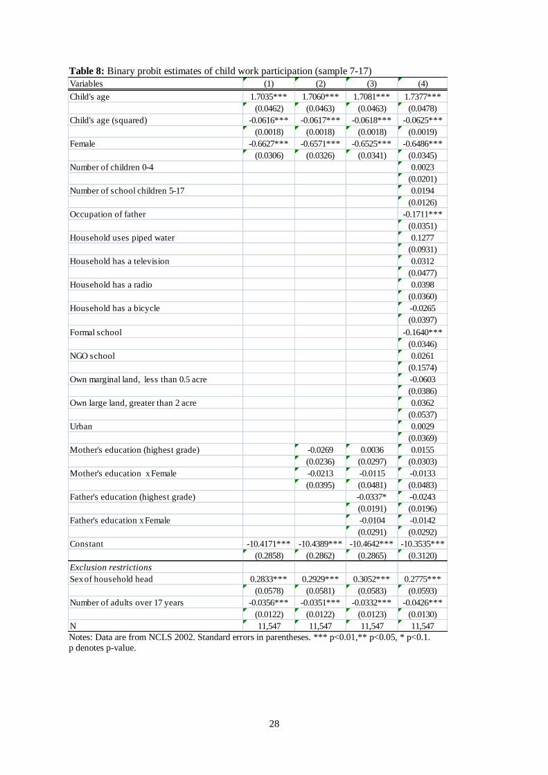
28

Table 8: Binary probit estimates of child work participation (sample 7-17)

Notes: Data are from NCLS 2002. Standard errors in parentheses. *** p<0.01,** p<0.05, * p<0.1.

p denotes p-value.

Variables (1) (2) (3) (4)

Child's age 1.7035*** 1.7060*** 1.7081*** 1.7377***

(0.0462) (0.0463) (0.0463) (0.0478)

Child's age (squared) -0.0616*** -0.0617*** -0.0618*** -0.0625***

(0.0018) (0.0018) (0.0018) (0.0019)

Female -0.6627*** -0.6571*** -0.6525*** -0.6486***

(0.0306) (0.0326) (0.0341) (0.0345)

Number of children 0-4 0.0023

(0.0201)

Number of school children 5-17 0.0194

(0.0126)

Occupation of father -0.1711***

(0.0351)

Household uses piped water 0.1277

(0.0931)

Household has a television 0.0312

(0.0477)

Household has a radio 0.0398

(0.0360)

Household has a bicycle -0.0265

(0.0397)

Formal school -0.1640***

(0.0346)

NGO school 0.0261

(0.1574)

Own marginal land, less than 0.5 acre -0.0603

(0.0386)

Own large land, greater than 2 acre 0.0362

(0.0537)

Urban 0.0029

(0.0369)

Mother's education (highest grade) -0.0269 0.0036 0.0155

(0.0236) (0.0297) (0.0303)

Mother's education x Female -0.0213 -0.0115 -0.0133

(0.0395) (0.0481) (0.0483)

Father's education (highest grade) -0.0337* -0.0243

(0.0191) (0.0196)

Father's education x Female -0.0104 -0.0142

(0.0291) (0.0292)

Constant -10.4171*** -10.4389*** -10.4642*** -10.3535***

(0.2858) (0.2862) (0.2865) (0.3120)

Exclusion restrictions

Sex of household head 0.2833*** 0.2929*** 0.3052*** 0.2775***

(0.0578) (0.0581) (0.0583) (0.0593)

Number of adults over 17 years -0.0356*** -0.0351*** -0.0332*** -0.0426***

(0.0122) (0.0122) (0.0123) (0.0130)

N 11,547 11,547 11,547 11,547

29

Table 9: Selectivity-adjusted and double-hurdle estimates of GAGE (sample 7-17)

Notes: Data are from NCLS 2002. Robust standard errors are in parenthesis. In Columns 7-8, the variables included but not reported are number of children 0-4, number

of school children 5-17, dummies for urban areas, occupation of the father and dwelling characteristics and facilities enjoyed by the household, dummies for

household ownership of land (for example, own marginal land, less than 0.5 acre; own large land, greater than 2 acre) and communal characteristics (for example,

presence of formal and NGO schools).*** p<0.01,** p<0.05, * p<0.1. p denotes p-value.

(1) (2) (3) (4) (5) (6) (7) (8)

Variables Selectivity-

adjusted

Double-Hurdle Selectivity-

adjusted

Double-Hurdle Selectivity-

adjusted

Double-Hurdle Selectivity-

adjusted

Double-Hurdle

Child's age 15.8681*** -15.4236*** 15.2708*** -15.7261*** 14.9260*** -15.8054*** 10.5176*** -15.0215***

(2.6792) (1.1001) (2.6459) (1.0714) (2.6409) (1.0667) (2.7560) (1.1041)

Child's age (squared) -0.5766*** 0.5464*** -0.5575*** 0.5542*** -0.5456*** 0.5556*** -0.3884*** 0.5198***

(0.0972) (0.0449) (0.0958) (0.0427) (0.0955) (0.0424) (0.0981) (0.0401)

Female -9.9633*** -0.4820 -10.3028*** -1.1342 -10.2306*** -1.3578 -8.4159*** -0.9949

(0.9830) (0.6944) (1.0065) (0.7801) (1.0252) (0.8436) (1.1177) (0.9541)

Child labour hours -1.1476** -1.3851** -0.9612* -1.1436 -0.9286* -1.0946 -0.8882 -0.9108

(0.5172) (0.6796) (0.5367) (0.6983) (0.5463) (0.7098) (0.5804) (0.7444)

Child labour hours (squared) 0.0136** 0.0164* 0.0110 0.0131 0.0106 0.0125 0.0105 0.0106

(0.0066) (0.0087) (0.0069) (0.0090) (0.0070) (0.0091) (0.0075) (0.0096)

Residual_child labour hours 1.0305** 1.3001* 0.8823 1.1047 0.8575 1.0651 0.8599 0.9205

(0.5184) (0.6811) (0.5378) (0.6997) (0.5473) (0.7112) (0.5814) (0.7457)

Residual_child labour hours (squared) -0.0130* -0.0163* -0.0107 -0.0134 -0.0104 -0.0129 -0.0107 -0.0114

(0.0066) (0.0087) (0.0069) (0.0090) (0.0070) (0.0091) (0.0075) (0.0096)

Mother's education (highest grade) 0.4819 0.8548* 0.5601* 0.6000 0.6968*** 0.6688**

(0.3736) (0.4750) (0.2992) (0.3724) (0.2610) (0.3165)

Mother's education x Female 1.0563** 1.7433*** 1.0476** 1.1979** 1.0674** 1.1354**

(0.4430) (0.5287) (0.4796) (0.5658) (0.4893) (0.5752)

Father's education (highest grade) -0.0533 0.3242 0.1343 0.3745*

(0.2129) (0.2638) (0.1653) (0.1987)

Father's education x Female 0.0144 0.5794 0.1257 0.4987

(0.3138) (0.3749) (0.3099) (0.3679)

Constant -113.9558*** 148.6462*** -111.6896*** 147.5952*** -109.2735*** 147.4900*** -55.8434** 153.8724***

(22.8025) (11.1280) (22.4931) (10.7941) (22.4470) (10.8124) (22.7719) (10.1527)

inverse Mill's ratio 140.5323*** 138.7977*** 137.3378*** 108.2542***

(11.8816) (11.7061) (11.6661) (11.5912)

Sigma 11.9150*** 11.7560*** 11.7223*** 11.6247***

(0.1557) (0.1524) (0.1517) (0.1497)

N 5,268 5,268 5,268 5,268 5,268 5,268 5,268 5,268

30

Table 10: Marginal effects of IV probit estimates of school attendance for child wage

(paid) employee (sample 5-17)

Notes: Data are from NCLS 2002. Standard errors in parentheses. In Columns 1-3, the variables

included but not reported are child’s age (in years) and its square term, sex of child, in Column

4, the variables included but not reported are child’s age (in years) and its square term, sex of child,

number of children 0-4, number of school children 5-17, number of adult males and females over

17 years, dummies for urban areas, occupation of the father and dwelling characteristics and facilities

enjoyed by the household, dummies for household ownership of land (for example, own marginal land,

less than 0.5 acre; own large land, greater than 2 acre) and communal characteristics (for example, presence of formal and NGO schools). *** p<0.01,** p<0.05, * p<0.1. p denotes p-value.

Table 11: Marginal effects of IV tobit estimates of school attendance for child wage (paid) employee (sample 7-17)

Notes: Data are from NCLS 2002. Standard errors in parentheses. In Columns 1-3, the variables

included but not reported are child’s age (in years) and its square term, sex of child, in Column

4, the variables included but not reported are child’s age (in years) and its square term, sex of child,

number of children 0-4, number of school children 5-17, number of adult males and females over

17 years, dummies for urban areas, occupation of the father and dwelling characteristics and facilities

enjoyed by the household, dummies for household ownership of land (for example, own marginal land,

less than 0.5 acre; own large land, greater than 2 acre) and communal characteristics (for example,

presence of formal and NGO schools). *** p<0.01,** p<0.05, * p<0.1. p denotes p-value.

(1) (2) (3) (4)

Variables ME ME ME ME

Child labour hours -0.0568*** -0.0568*** -0.0560*** -0.0283***

(0.0173) (0.0172) (0.0171) (0.0074)

Child labour hours (squared) 0.0006*** 0.0006*** 0.0006*** 0.0003***

(0.0002) (0.0002) (0.0002) (0.0001)

Residual_child labour hours 0.0439** 0.0440** 0.0431** 0.0234***

(0.0173) (0.0173) (0.0171) (0.0073)

Residual_child labour hours (squared) -0.0005*** -0.0005*** -0.0005*** -0.0003***

(0.0002) (0.0002) (0.0002) (0.0001)

Mother's education (highest grade) 0.0309** 0.0245* 0.0000

(0.0122) (0.0128) (0.0055)

Mother's education x Female 0.0195 -0.0293 -0.0121

(0.0295) (0.0338) (0.0141)

Father's education (highest grade) 0.0125 -0.0021

(0.0076) (0.0035)

Father's education x Female 0.0650*** 0.0347***

(0.0234) (0.0104)

N 3,246 3,246 3,246 3,246

(1) (2) (3) (4)

Variables ME ME ME ME

Child labour hours -0.0805 -0.0731 -0.0773 -0.2249

(0.3007) (0.2986) (0.2963) (0.2143)

Child labour hours (squared) 0.0021 0.0019 0.0018 0.0027

(0.0035) (0.0035) (0.0034) (0.0025)

Residual_child labour hours -0.0188 -0.0189 -0.0145 0.2325

(0.3021) (0.3000) (0.2977) (0.2156)

Residual_child labour hours (squared) -0.0015 -0.0014 -0.0013 -0.0028

(0.0035) (0.0035) (0.0034) (0.0025)

Mother's education (highest grade) 1.8027*** 1.1966*** 0.1359

(0.2646) (0.2745) (0.2136)

Mother's education x Female 0.4543 -0.2976 0.5055

(0.6475) (0.7308) (0.5778)

Father's education (highest grade) 1.0612*** 0.1688

(0.1536) (0.1225)

Father's education x Female -0.2976 0.5055

(0.7308) (0.5778)

N 3,236 3,236 3,236 3,236

31

Table 12: Marginal effects of IV probit estimates of school attendance, by urban location

(sample 5-17)

Notes: Data are from NCLS 2002. Standard errors in parentheses. In Columns 1-3, the variables

included but not reported are child’s age (in years) and its square term, sex of child, in Column

4, the variables included but not reported are child’s age (in years) and its square term, sex of child,

number of children 0-4, number of school children 5-17, number of adult males and females over

17 years, occupation of the father and dwelling characteristics and facilities enjoyed by the household,

dummies for household ownership of land (for example, own marginal land, less than 0.5 acre; own large land, greater than 2 acre) and communal characteristics (for example, presence of formal and NGO schools).

*** p<0.01,** p<0.05, * p<0.1. p denotes p-value.

Table 13: Marginal effects of IV probit estimates of school attendance, by rural location (sample 5-17)

Notes: Data are from NCLS 2002. Standard errors in parentheses. In Columns 1-3, the variables

included but not reported are child’s age (in years) and its square term, sex of child, in Column

4, the variables included but not reported are child’s age (in years) and its square term, sex of child,

number of children 0-4, number of school children 5-17, number of adult males and females over

17 years, occupation of the father and dwelling characteristics and facilities enjoyed by the household,

dummies for household ownership of land (for example, own marginal land, less than 0.5 acre; own large land, greater than 2 acre) and communal characteristics (for example, presence of formal and NGO schools).

*** p<0.01,** p<0.05, * p<0.1. p denotes p-value.

(1) (2) (3) (4)

Variables ME ME ME ME

Child labour hours -0.0785*** -0.0796*** -0.0845*** -0.0530**

(0.0268) (0.0275) (0.0279) (0.0217)

Child labour hours (squared) 0.0008** 0.0008** 0.0009** 0.0006**

(0.0003) (0.0003) (0.0004) (0.0003)

Residual_child labour hours 0.0444* 0.0474* 0.0528* 0.0323

(0.0269) (0.0275) (0.0279) (0.0216)

Residual_child labour hours (squared) -0.0005 -0.0006* -0.0006* -0.0004

(0.0003) (0.0003) (0.0004) (0.0003)

Mother's education (highest grade) 0.0722*** 0.0573*** 0.0149

(0.0192) (0.0171) (0.0125)

Mother's education x Female 0.0025 -0.0368 -0.0303

(0.0250) (0.0317) (0.0248)

Father's education (highest grade) 0.0155 0.0026

(0.0135) (0.0095)

Father's education x Female 0.0500** 0.0437**

(0.0212) (0.0173)

N 2,508 2,508 2,508 2,508

Urban Sample

(1) (2) (3) (4)

Variables ME ME ME ME

Child labour hours -0.0804*** -0.0706** -0.0605** -0.0594***

(0.0282) (0.0294) (0.0297) (0.0220)

Child labour hours (squared) 0.0008** 0.0007* 0.0006 0.0007**

(0.0004) (0.0004) (0.0004) (0.0003)

Residual_child labour hours 0.0411 0.0326 0.0228 0.0366*

(0.0283) (0.0295) (0.0298) (0.0220)

Residual_child labour hours (squared) -0.0005 -0.0004 -0.0002 -0.0005*

(0.0004) (0.0004) (0.0004) (0.0003)

Mother's education (highest grade) 0.0895*** 0.0555*** 0.0109

(0.0217) (0.0187) (0.0125)

Mother's education x Female 0.0454* 0.0337 0.0142

(0.0257) (0.0266) (0.0202)

Father's education (highest grade) 0.0543*** 0.0069

(0.0106) (0.0064)

Father's education x Female -0.0008 0.0117

(0.0166) (0.0123)

N 6,392 6,392 6,392 6,392

Rural Sample

32

Table 14: Marginal effects of IV tobit estimates of GAGE, by urban location

(sample 7-17)

Notes: Data are from NCLS 2002. Standard errors in parentheses. In Columns 1-3, the variables

included but not reported are child’s age (in years) and its square term, sex of child, in Column

4, the variables included but not reported are child’s age (in years) and its square term, sex of child,

number of children 0-4, number of school children 5-17, number of adult males and females over

17 years, occupation of the father and dwelling characteristics and facilities enjoyed by the household, dummies for household ownership of land (for example, own marginal land, less than 0.5 acre; own large

land, greater than 2 acre) and communal characteristics (for example, presence of formal and NGO schools).

*** p<0.01,** p<0.05, * p<0.1. p denotes p-value.

Table 15: Marginal effects of IV tobit estimates of GAGE, by rural location (sample 7-17)

Notes: Data are from NCLS 2002. Standard errors in parentheses. In Columns 1-3, the variables included but not reported are child’s age (in years) and its square term, sex of child, in Column 4,

the variables included but not reported are child’s age (in years) and its square term, sex of child,

number of children 0-4, number of school children 5-17, number of adult males and females over

17 years, occupation of the father and dwelling characteristics and facilities enjoyed by the household,

dummies for household ownership of land (for example, own marginal land, less than 0.5 acre; own large

land, greater than 2 acre) and communal characteristics (for example, presence of formal and NGO schools).

*** p<0.01,** p<0.05, * p<0.1. p denotes p-value.

(1) (2) (3) (4)

Variables ME ME ME ME

Child labour hours -0.1492 -0.0448 -0.4198*** 0.2141

(0.4134) (0.4097) (0.0710) (0.3313)

Child labour hours (squared) 0.0008 -0.0003 0.0036*** -0.0032

(0.0052) (0.0051) (0.0007) (0.0041)

Residual_child labour hours -0.2005 -0.2340 0.1504** -0.2872

(0.4149) (0.4111) (0.0654) (0.3325)

Residual_child labour hours (squared) 0.0020 0.0026 -0.0014** 0.0037

(0.0052) (0.0052) (0.0006) (0.0042)

Mother's education (highest grade) 2.6152*** 1.8785*** 0.8473***

(0.3024) (0.3000) (0.2167)

Mother's education x Female -0.0095 0.6437 -0.1858

(0.4120) (0.4567) (0.4134)

Father's education (highest grade) 0.8121*** 0.2479

(0.2116) (0.1541)

Father's education x Female 0.4684 -0.1858

(0.3271) (0.4134)

N 2,497 2,497 2,497 2,497

Urban Sample

(1) (2) (3) (4)

Variables ME ME ME ME

Child labour hours -0.9358** -0.7316* -0.5762 -0.3504

(0.3724) (0.3804) (0.3836) (0.3138)

Child labour hours (squared) 0.0117** 0.0089* 0.0069 0.0042

(0.0050) (0.0051) (0.0051) (0.0041)

Residual_child labour hours 0.5751 0.4118 0.2692 0.3604

(0.3733) (0.3813) (0.3844) (0.3146)

Residual_child labour hours (squared) -0.0083* -0.0059 -0.0040 -0.0044

(0.0050) (0.0051) (0.0051) (0.0041)

Mother's education (highest grade) 1.9368*** 0.9654*** 0.3535*

(0.2943) (0.2635) (0.1997)

Mother's education x Female 1.6773*** 1.5939*** 0.9449***

(0.3960) (0.4289) (0.3585)

Father's education (highest grade) 1.3185*** 0.2077*

(0.1532) (0.1086)

Father's education x Female -0.1100 0.1969

(0.2615) (0.2147)

N 6,351 6,351 6,351 6,351

Rural Sample

33

Acknowledgements

We are benefitted from comments by participants at the Monday workshop at Monash University and

participants at the Australian Conference of Economists and at the Australasian Development

Economics workshop. We also gratefully acknowledge funding from Monash University, Australia (Postgraduate publications award). The usual caveat applies.

34

References

Akabayashi H, Psacharopoulos G (1999) The Trade-off between Child Labour and Human Capital

Formation: A Tanzanian Case Study. Journal of Development Studies 35(5): 120-140.

Amin S, Quayes M S, Rives J M (2006) Market Work and Household Work as Deterrents to

Schooling in Bangladesh. World Development 34(7): 1271-1286. Arends-Kuenning M, Amin S (2004) School Incentive Programs and Children's Activities: The Case

of Bangladesh. Comparative Education Review 48(3): 295-317.

Aristei D, Perali F, Pieroni L (2008) Cohort, Age and Time Effects in Alcohol Consumption by Italian Households: A Double-Hurdle Approach. Empirical Economics 35(1): 29-61.

Basu K (1999) Child Labor: Cause, Consequence, and Cure, with Remarks on International Labor

Standards. Journal of Economic Literature 37(3): 1083-1119. Basu K (2006) Gender and Say: A Model of Household Behaviour with Endogenously Determined

Balance of Power. The Economic Journal 116(511): 558-580.

Basu K, Ray R (2001) The Collective Model of the Household and An Unexpected Implication for

Child Labor: Hypothesis and an Empirical Test. Working Paper 2813. World Bank, Washington DC.

Basu K, Tzannatos Z (2003) The Global Child Labor Problem: What Do We Know and What Can We

Do? The World Bank Economic Review 17(2): 147-173. Basu K, Van P H (1998) The Economics of Child Labor. American Economic Review 88(3): 412-

427.

Beegle K, Dehejia R, Gatti R (2009) Why Should We Care about Child Labor? Journal of Human Resources 44(4): 871-889.

Bhalotra S (2007) Is Child Work Necessary? Oxford Bulletin of Economics and Statistics 69(1): 29-

55.

Boozer M, Suri T (2001) Child Labor and Schooling Decisions in Ghana. Mimeo, CT: Yale University.

Coulombe H (1998) Child Labour and Education in Cote d' Ivore. Mimeo, World Bank D.P.

Cragg J G (1971) Some Statistical Models for Limited Dependent Variables with Application to the Demand for Durable Goods. Econometrica 39(5): 829-844.

Dar A, Blunch N-H, Kim B, Sasaki M (2002) Participation of Children in Schooling and Labor

Activities: A Review of Empirical Studies. Social Protection D.P. 0221. World Bank,

Washington DC. Deb P, Rosati F (2002) Determinants of Child Labor and School Attendance: The Role of Household

Unobservables. Understanding Children's Work Research Paper.

Edmonds E V (2007) Child Labour. In: Scultz T P, Strauss, J (eds) The Handbook of Development Economics, (vol. 4 ). Amsterdam: North Holland.

Emerson P M, Souza A P (2003) Is there a Child Labor Trap? Intergenerational Persistence of Child

Labor in Brazil. Economic Development and Cultural Change 51(2): 375-398. Emerson P M, Souza A P (2007) Child Labor, School Attendance, and Intrahousehold Gender Bias in

Brazil. The World Bank Economic Review 21(2): 301-316.

Ersado L (2005) Child Labor and Schooling Decisions in Urban and Rural Areas: Comparative

Evidence from Nepal, Peru, and Zimbabwe. World Development 33(3): 455-480. Ganglmair B (2006) Intrinsic Competition and the Labor-Schooling Trade-off in Uganda. Working

Paper, Econ WPA.

Goulart P, Bedi A S (2008) Child Labour and Educational Success in Portugal. Economics of Education Review 27(5): 575-587.

Green W H (1997) Econometric Analysis. 3rd ed, Prentice-Hall, Inc.

Grootaert C (1999) Child Labor in Cote d' Ivore: Incidence and Determinants. In: Grootaert C, Patrinos, H (eds) The Policy Analysis of Child Labor: A Comparative Study, New York: St.

Martin's Press.

Guarcello L, Lyon S, Rosati F (2006) Child Labour and Education for All: An Issue Paper.

Understanding Children's Work Project Working Paper Series, November. Gunnarsson V, Orazem P F, Sánchez M A (2006) Child Labor and School Achievement in Latin

America. The World Bank Economic Review 20(1): 31-54.

35

Han P (2008) Human Capital and Hours Worked of Children in Cambodia: Empirical Evidence for

Policy Implications. Asian Economic Journal 22(1): 25-46. Heady C (2003) The Effect of Child Labor on Learning Achievement. World Development 31(2):

385-398.

Islam A, Choe C (2011) Child Labour and Schooling Responses to Access to Microcredit in Rural

Bangladesh. Economic Inquiry, forthcoming. Jensen P, Nielsen H S (1997) Child Labour or School Attendance? Evidence from Zambia. Journal of

Population Economics 10(4): 407-424.

Jones A M (1989) A Double-Hurdle Model of Cigarette Consumption. Journal of Applied Econometrics 4(1): 23-39.

Kana M, Phoumin H, Seiichi F (2010) Does Child Labour Have a Negative Impact on Child

Education and Health? A Case Study in Rural Cambodia. Oxford Development Studies 38(3): 357-382.

Khanam R (2006) Child Labour in Bangladesh: Trends, Patterns and Policy Options. Asian Profile

34(6): 1-33.

Khanam R (2008) Child Labour and School Attendance: Evidence from Bangladesh. International Journal of Social Economics 35(1/2): 77-98.

Maitra P, Ray R (2002) The Joint Estimation of Child Participation in Schooling and Employment:

Comparative Evidence from Three Continents. Oxford Development Studies 30(1): 41-62. McElroy M B, Horney M J (1981) Nash-Bargained Household Decisions: Toward a Generalization of

the Theory of Demand. International Economic Review 22(2): 333-349.

NCLS (2002) Report on the National Child Labour Survey. Bangladesh Bureau of Statistics, Dhaka:Bangladesh.

Parikh A, Sadoulet E (2005) The Effects of Parents' Occupation on Child Labour and School

Attendance in Brazil. Mimeo, Univesity of California at Berkeley.

Patrinos H A, Psacharopoulos G (1995) Educational Performance and Child Labor in Paraguay. International Journal of Educational Development 15(1): 47-60.

Patrinos H A, Psacharopoulos G (1997) Family Size, Schooling and Child Labor in Peru: An

Empirical Analysis. Journal of Population Economics 10(4): 387-405. Psacharopoulos G, Yang H (1991) Educational Attainment among Venezuelan Youth: An Analysis of

its Determinants. International Journal of Educational Development 11(4): 289-294.

Rahman M M, Khanam R, Absar N U (1999) Child Labor in Bangladesh: A Critical Appraisal of

Harkin's Bill and the MOU-Type Schooling Program. Journal of Economic Issues 33(4): 985-1003.

Rammohan A (2012) The Trade-off between Child Labour and Schooling in India. Education

Economics, forthcoming. Ravallion M, Wodon Q (2000) Does Child Labour Displace Schooling? Evidence on Behavioural

Responses to an Enrollment Subsidy. The Economic Journal 110(462): 158-175.

Ray R (2000a) Analysis of Child Labour in Peru and Pakistan: A Comparative Study. Journal of Population Economics 13(1): 3-19.

Ray R (2000b) Poverty, Household Size and Child Welfare in India. Economic and Political Weekly

35(39): 3511-3520.

Ray R (2002) Simultaneous Analysis of Child Labour and Child Schooling: Comparative Evidence from Nepal and Pakistan. Economic and Political Weekly 37(52): 5215-5224.

Ray R, Lancaster G (2005) The Impact of Children's Work on Schooling: Multi-Country Evidence.

International Labour Review 144(2): 189-210. Ridao-Cano C (2001) Child Labor and Schooling in a Low Income Rural Economy. Population Aging

Center Working Paper PAC 2001-0001, Institute of Behavioral Science, University of

Colorado at Boulder. Rosati F, Rossi M (2003) Children's Working Hours and School Enrollment: Evidence from Pakistan

and Nicaragua. The World Bank Economic Review 17(2): 283-295.

Sedlacek G, Duryea S, Ilahi N, Sasaki M (2009) Child Labour, Schooling and Poverty in Latin

America. In: Orazem P F, Sedlacek G, Tzannatos Z (eds) Child Labour and Education in Latin America: An Economic Perspective, Palgrave Macmillan.

36

Shafiq M N (2007) Household Schooling and Child Labor Decisions in Rural Bangladesh. Journal of

Asian Economics 18(6): 946-966. Udry C (2006) Child Labour. In: Banerjee A V, Benabou R, Mookherjee D (Eds) Understanding

Poverty, New York, Oxford University Press.

Van De Ven W P M M, Van Praag B M S (1981) The Demand for Deductibles in Private Health

Insurance : A Probit Model with Sample Selection. Journal of Econometrics 17(2): 229-252. Wahba J (2006) The Influence of Market Wages and Parental History on Child Labour and Schooling

in Egypt. Journal of Population Economics 19(4): 823-852.

Zabaleta M B (2011) The Impact of Child Labor on Schooling Outcomes in Nicaragua. Economics of Education Review 30(6): 1527-1539.

37

Appendix

Table A1: First stage OLS estimates of child labour hours (sample 5-17)

Continued on next page

Variables Child labour

hours

Child labour

hours2

Child labour

hours

Child labour

hours2

Child labour

hours

Child labour

hours2

Child labour

hours

Child labour

hours2

Child's age -4.6797*** -364.2844*** -4.2318*** -335.8697*** -4.1576*** -331.1257*** -2.6349*** -239.3926***

(0.5685) (45.3490) (0.5627) (45.0852) (0.5611) (45.0095) (0.5543) (44.8632)

Child's age (squared) 0.2537*** 18.2197*** 0.2361*** 17.0991*** 0.2337*** 16.9498*** 0.1838*** 13.9708***

(0.0217) (1.7345) (0.0215) (1.7246) (0.0215) (1.7216) (0.0212) (1.7121)

Female -7.8234*** -558.0371*** -8.3044*** -587.3813*** -8.6962*** -612.1867*** -9.1009*** -639.4684***

(0.3671) (29.2830) (0.3869) (30.9968) (0.4037) (32.3822) (0.3951) (31.9826)

Number of children 0-4 0.5522*** 39.4679**

(0.2064) (16.7104)

Number of school children 5-17 0.3561*** 21.5989**

(0.1263) (10.2205)

Number of adult males over 17 years -0.2842 -17.6645

(0.2043) (16.5361)

Number of adult females over 17 years -0.3300 -24.3213

(0.2593) (20.9867)

Occupation of father -1.6757*** -127.0299***

(0.4063) (32.8828)

Household uses piped water 5.2520*** 440.8984***

(0.9445) (76.4504)

Household has a TV -1.9084*** -102.5120***

(0.4732) (38.2988)

Household has a radio 0.0424 -8.8819

(0.3497) (28.3014)

Household has a bicycle -1.9197*** -143.8875***

(0.3819) (30.9097)

Formal school 2.4040*** 149.1312***

(0.3807) (30.8143)

NGO school -0.1983 8.9358

(0.5056) (40.9233)

Own marginal land, less than 0.5 acre -4.7312*** -282.1031***

(0.3285) (26.5927)

Own large land, greater than 2 acre -6.6715*** -498.2775***

(1.5208) (123.0984)

Urban -1.4713*** -149.3000***

(0.3813) (30.8615)

(1) (2) (3) (4)

38

Table A1 (continued): First stage OLS estimates of child labour hours (sample 5-17)

Notes: Data are from NCLS 2002. Standard errors in parentheses. *** p<0.01,** p<0.05, * p<0.1. p denotes p-value.

Variables Child labour

hours

Child labour

hours2

Child labour

hours

Child labour

hours2

Child labour

hours

Child labour

hours2

Child labour

hours

Child labour

hours2

Mother's education (highest grade) -3.1184*** -197.2523*** -1.7419*** -1.8912*** -1.4778*** -98.2428***

(0.2211) (17.7113) (0.3227) (0.2736) (0.2694) (21.8069)

Mother's education x Female 1.5313*** 92.9690** 0.4469 0.5108 0.8163 48.1522

(0.4776) (38.2628) (0.6692) (0.5754) (0.5606) (45.3733)

Father's education (highest grade) -1.4409*** -1.3730*** -0.6711*** -45.9580***

(0.1974) (0.1815) (0.1809) (14.6401)

Father's education x Female 1.1887*** 1.1531*** 1.0188*** 65.1151**

(0.3729) (0.3476) (0.3388) (27.4260)

Agriculture -10.6330*** -712.9078*** -10.4795*** -703.2634*** -10.3606*** -694.7708*** -9.4509*** -630.3137***

(0.8604) (68.6288) (0.8505) (68.1382) (0.8483) (68.0233) (0.8593) (69.5562)

Manufacturing 1.0169 199.9034*** 1.2118 212.0977*** 1.3700 222.6538*** 1.6431* 235.4989***

(0.9168) (73.1279) (0.9064) (72.6169) (0.9044) (72.5158) (0.8818) (71.3771)

Wholesale and Retail -1.8629** -17.7724 -1.3689 13.5565 -1.2142 23.8175 -0.7314 54.8788

(0.8889) (70.9055) (0.8792) (70.4402) (0.8770) (70.3249) (0.8565) (69.3256)

Services -2.3840** -68.2391 -1.9527* -40.6452 -1.8156 -32.0466 -1.3494 -6.4719

(1.1652) (92.9469) (1.1524) (92.3259) (1.1496) (92.1957) (1.1205) (90.6986)

Constant 51.9231*** 3,077.5452*** 49.8776*** 2,947.6196*** 49.6883*** 2,932.3314*** 43.8524*** 2,718.9261***

(3.7588) (299.8323) (3.7178) (297.8616) (3.7076) (297.3305) (3.8030) (307.8235)

F -test on instruments 257.13 244.74 271.15 254.7 256.45 273.69 149.68 137.15

p>F (p = 0.0000) (p = 0.0000) (p = 0.0000) (p = 0.0000) (p = 0.0000) (p = 0.0000) (p = 0.0000) (p = 0.0000)

Adj. R-squared 0.24 0.20 0.26 0.21 0.21 0.26 0.30 0.24

N 8,900 8,900 8,900 8,900 8,900 8,900 8,900 8,900

(1) (2) (3) (4)

39

Table A2: First stage OLS estimates of child labour hours (sample 7-17)

Continued on next page

Variables Child labour

hours

Child labour

hours2

Child labour

hours

Child labour

hours2

Child labour

hours

Child labour

hours2

Child labour

hours

Child labour

hours2

Child's age -5.8860*** -444.9689*** -5.1783*** -400.1323*** -5.0317*** -390.8067*** -3.0480*** -269.9108***

(0.7151) (57.1144) (0.7086) (56.8410) (0.7067) (56.7590) (0.6973) (56.5286)

Child's age (squared) 0.2973*** 21.1350*** 0.2703*** 19.4209*** 0.2653*** 19.1054*** 0.1988*** 15.0732***

(0.0268) (2.1423) (0.0266) (2.1322) (0.0265) (2.1290) (0.0261) (2.1165)

Female -7.8539*** -561.0331*** -8.3566*** -591.6035*** -8.7422*** -616.3955*** -9.1892*** -646.1983***

(0.3687) (29.4485) (0.3888) (31.1860) (0.4056) (32.5745) (0.3969) (32.1717)

Number of children 0-4 0.5578*** 39.2850**

(0.2073) (16.8088)

Number of school children 5-17 0.3476*** 21.0636**

(0.1267) (10.2699)

Number of adult males over 17 years -0.2984 -18.6911

(0.2043) (16.5629)

Number of adult females over 17 years -0.3478 -25.4499

(0.2593) (21.0209)

Occupation of father -1.7000*** -129.1848***

(0.4071) (32.9996)

Household uses piped water 5.2083*** 437.4386***

(0.9434) (76.4765)

Household has a television -1.8963*** -101.9894***

(0.4729) (38.3332)

Household has a radio 0.0127 -10.5106

(0.3502) (28.3876)

Household has a bicycle -1.8823*** -140.8615***

(0.3825) (31.0064)

Formal school -4.7858*** -285.2718***

(0.3289) (26.6612)

(1) (2) (3) (4)

40

Table A2 (continued): First stage OLS estimates of child labour hours (sample 7-17)

Notes: Data are from NCLS 2002. Standard errors in parentheses. *** p<0.01,** p<0.05, * p<0.1. p denotes p-value.

Variables Child labour

hours

Child labour

hours2

Child labour

hours

Child labour

hours2

Child labour

hours

Child labour

hours2

Child labour

hours

Child labour

hours2

NGO school -6.7112*** -500.8623***

(1.5187) (123.1178)

Own marginal land, less than 0.5 acre 2.4325*** 151.3531***

(0.3811) (30.8972)

Own large land, greater than 2 acre -0.2411 6.2245

(0.5069) (41.0905)

Urban -1.5230*** -153.6383***

(0.3816) (30.9355)

Mother's education (highest grade) -3.1084*** -196.3802*** -1.8727*** -117.5719*** -1.4635*** -97.2046***

(0.2220) (17.8122) (0.2756) (22.1328) (0.2712) (21.9818)

Mother's education x Female 1.5734*** 95.1152** 0.5576 29.7853 0.8737 50.2085

(0.4794) (38.4607) (0.5778) (46.4095) (0.5627) (45.6130)

Father's education (highest grade) -1.3732*** -87.5733*** -0.6663*** -45.7605***

(0.1824) (14.6467) (0.1816) (14.7200)

Father's education x Female 1.1380*** 73.1562*** 1.0129*** 65.7800**

(0.3489) (28.0181) (0.3398) (27.5488)

Agriculture -10.5471*** -703.6908*** -10.3962*** -694.2360*** -10.2658*** -685.9097*** -9.3371*** -619.2119***

(0.8624) (68.8775) (0.8526) (68.3943) (0.8501) (68.2791) (0.8610) (69.8000)

Manufacturing 1.1056 210.0515*** 1.3057 222.5491*** 1.4666 232.8447*** 1.7605** 247.5094***

(0.9187) (73.3763) (0.9084) (72.8743) (0.9061) (72.7728) (0.8834) (71.6150)

Wholesale and Retail -1.7863** -8.5738 -1.2984 22.3474 -1.1330 32.8950 -0.6303 65.6976

(0.8907) (71.1440) (0.8812) (70.6859) (0.8787) (70.5721) (0.8580) (69.5570)

Services -2.3868** -63.3046 -1.9575* -35.8353 -1.8249 -27.4401 -1.3162 0.7437

(1.1669) (93.1979) (1.1542) (92.5885) (1.1511) (92.4507) (1.1217) (90.9281)

Constant 60.0304*** 3,616.7075*** 56.2252*** 3,375.4621*** 55.4972*** 3,329.1966*** 46.7709*** 2,932.4285***

(4.7689) (380.8950) (4.7215) (378.7573) (4.7083) (378.1515) (4.7505) (385.1002)

F -test on instruments 255.28 242.82 269.24 252.72 271.88 254.56 148.69 136.14

p>F (p = 0.0000) (p = 0.0000) (p = 0.0000) (p = 0.0000) (p = 0.0000) (p = 0.0000) (p = 0.0000) (p = 0.0000)

Adj. R-squared 0.24 0.20 0.26 0.21 0.26 0.21 0.30 0.24

N 8,848 8,848 8,848 8,848 8,848 8,848 8,848 8,848

(1) (2) (3) (4)