(This is a sample cover image for this issue. The actual ... vertically forced pendulum or the...

(This is a sample cover image for this issue. The actual cover is not yet available at this time.)

This article appeared in a journal published by Elsevier. The attachedcopy is furnished to the author for internal non-commercial researchand education use, including for instruction at the authors institution

and sharing with colleagues.

Other uses, including reproduction and distribution, or selling orlicensing copies, or posting to personal, institutional or third party

websites are prohibited.

In most cases authors are permitted to post their version of thearticle (e.g. in Word or Tex form) to their personal website orinstitutional repository. Authors requiring further information

regarding Elsevier’s archiving and manuscript policies areencouraged to visit:

http://www.elsevier.com/copyright

http://www.elsevier.com/copyright

Author's personal copy

Non-smooth stability analysis of the parametrically excited impact oscillator

R.I. Leine

Institute of Mechanical Systems, Department of Mechanical and Process Engineering, ETH Zurich, CH-8092 Zurich, Switzerland

a r t i c l e i n f o

Article history:

Received 29 September 2011

Accepted 24 June 2012Available online 30 June 2012

Keywords:

Parametric excitation

Non-smooth dynamics

Impulsive dynamics

Hill’s equation

a b s t r a c t

The aim of this paper is to give a Lyapunov stability analysis of a parametrically excited impact

oscillator, i.e. a vertically driven pendulum which can collide with a support. The impact oscillator with

parametric excitation is described by Hill’s equation with a unilateral constraint. The unilaterally

constrained Hill’s equation is an archetype of a parametrically excited non-smooth dynamical system

with state jumps. The exact stability criteria of the unilaterally constrained Hill’s equation are

rigorously derived using Lyapunov techniques and are expressed in the properties of the fundamental

solutions of the unconstrained Hill’s equation. Furthermore, an asymptotic approximation method for

the critical restitution coefficient is presented based on Hill’s infinite determinant and this approxima-

tion can be made arbitrarily accurate. A comparison of numerical and theoretical results is presented

for the unilaterally constrained Mathieu equation.

& 2012 Elsevier Ltd. All rights reserved.

1. Introduction

The objective of the paper is to give more insight into thestability properties of non-smooth dynamical systems with para-metric excitation. The impact oscillator with parametric excitationis studied which is described by Hill’s equation with a unilateralconstraint.

The theory of parametrically excited systems has applicationsin a wide range of disciplines, e.g. the quadrupole ion trap [19],the exact plane wave solutions in general relativity [3], para-metric amplifiers [1], rotor dynamical instabilities [23,24,28],parametric resonance in power transmission belts [20] andcelestial mechanics [25]. The importance of parametric excitationhas led to a wealth of literature on the theoretical and experi-mental analysis of parametrically excited systems, see [8,28] andreferences therein. The attention in the literature is mainlyfocussed on the dynamics of the planar vertically driven pendu-lum and on its linearization which is described by Hill’s equation.The vertically driven pendulum, of which the suspension point isdriven periodically up and down (see Fig. 1a), is one of thesimplest mechanical systems with parametric excitation. Thesystem is also known as the parametrically excited pendulum,the vertically forced pendulum or the Kapitza pendulum. Thedynamics of the vertically driven pendulum can (after somescaling) be expressed by

€WðtÞþg

l�

aðtÞ

l

� �sin WðtÞ ¼ 0, ð1Þ

where W is the angle of the pendulum with the downward verticaland aðtÞ ¼ €uðtÞ is the vertical acceleration of the suspension point.

Extensive studies of the non-linear dynamics of the verticallydriven pendulum can be found in [2,4,5,8,26]. The dynamics ofthe pendulum system in the vicinity of its equilibrium positionsW¼ 0 and W¼ p is described by Hill’s equation [6,17,30]

€yðtÞþgðtÞyðtÞ ¼ 0, ð2Þ

where gðtÞ ¼ gðtþpÞ is a real piece-wise continuous function.Harmonic excitation leads to the so-called Mathieu equation

€yðtÞþðaþ2b cos 2tÞyðtÞ ¼ 0, ð3Þ

being a special case of Hill’s equation with gðtÞ ¼ aþ2b cos 2t.Systems with some degree of non-smoothness or switching

behavior are often referred to as non-smooth dynamical systems[7,10,15]. Mechanical systems with impact and/or friction forman important subclass of non-smooth dynamical systems. Thestability properties of non-smooth (mechanical) systems arecurrently receiving much attention, see [16] and referencestherein. However, the stability of equilibria of parametricallyexcited non-smooth systems has hardly been addressed.

Following [22], various contributions study the dynamics ofthe planar pendulum with impact but with a horizontally drivensuspension point and the system is therefore not parametricallyexcited. Moreover, the existence of an equilibrium is lost underhorizontal excitation.

Ivanov [11] studies the dynamics of Hill’s equation with animpulsive parametric excitation in which the function g(t) con-tains Dirac functions. Although impulsive action is added to Hill’sequation, the linearity of the system is maintained.

Quinn [21] gives an in-depth study of two parametrically excitedpendula under vertical harmonic excitation which can collide witheach other. A symmetric response of the pendula agrees with thedynamics of a single vertically driven pendulum (1) with a unilateral

Contents lists available at SciVerse ScienceDirect

journal homepage: www.elsevier.com/locate/nlm

International Journal of Non-Linear Mechanics

0020-7462/$ - see front matter & 2012 Elsevier Ltd. All rights reserved.

http://dx.doi.org/10.1016/j.ijnonlinmec.2012.06.010

E-mail address: [email protected]

International Journal of Non-Linear Mechanics 47 (2012) 1020–1032


constraint at W¼ 0 and the impact law _Wþ¼ �e _W

�. The method of

averaging in amplitude and phase coordinates (Lagrange standardform) is used to describe the dynamics in the vicinity of theequilibrium and near a resonance frequency under the assumptionof a small amplitude of the excitation a(t). The analysis takes thenon-linearity of the pendulum into account using the approximationsin W� W� 1

6W3, that is to say, the ‘nonlinear Mathieu equation’

€yðtÞþðaþ2b cos 2tÞðyðtÞ� 16 yðtÞ3Þ ¼ 0 is considered. The averaged

equations of motion in amplitude and phase coordinates are usedto derive an approximate impact event map which maps the state ofthe system at a collision time instant to the state at the followingcollision time instant. The results in [21] can be used to derive anapproximate stability criterion for the equilibrium point of the(linear or non-linear) Mathieu equation with unilateral constraint.The drawback of the approach taken in [21] is that the approxima-tion is only valid for small values of the excitation parameter b andnear a chosen resonance frequency

ffiffiffiap¼ 1;2,3 . . ..

In this paper, a detailed Lyapunov stability analysis is pre-sented of the equilibrium of Hill’s equation in the presence of aunilateral constraint with restitution, hereafter called the (uni-laterally) constrained Hill’s equation. The aim of this paper istwofold. Firstly, the exact stability criteria of the unilaterallyconstrained Hill’s equation are rigorously derived using Lyapunovtechniques and are expressed in the properties of the fundamen-tal solutions of the unconstrained Hill’s equation (2). Secondly, anasymptotic approximation method for the critical restitutioncoefficient is presented based on Hill’s infinite determinant andthis approximation can be made arbitrarily accurate.

Hill’s equation in the presence of a unilateral constraint withrestitution is described by

€xðtÞþgðtÞxðtÞ ¼ 0,

xðtiÞ ¼ 0: _xþ ðtiÞ ¼�e _x�ðtiÞ, ð4Þ

where e is the restitution coefficient. The unilateral constraint limitsthe dynamics to xðtÞZ0 and imposes a Newtonian impact law_xþ ¼�e _x�. More physically correct would be to formulate theunilaterally constrained system (4) in the framework of non-smooth dynamics [7,10,15,16] and to let a contact force l and animpulsive contact force L (both per unit mass) appear in theequation of motion and impact equation as Lagrange multipliers, i.e.

€xðtÞþgðtÞxðtÞ ¼ l for almost all t,

xðtiÞ ¼ 0: _xþ ðtiÞ�_x�ðtiÞ ¼L, ð5Þ

together with the set-valued contact law (Signorini’s law)

0rl ? xZ0 ð6Þ

and the generalized Newtonian impact law

xðtiÞ ¼ 0: 0rL ? _xþ ðtiÞþe _x�ðtiÞZ0, ð7Þ

where 0ra ? bZ0 denotes the inequality complementarity con-dition aZ0, bZ0, ab¼0 [7,10,16]. Such a (mechanical) system withimpulsive effects due to unilateral constraints may be convenientlycast in terms of a measure differential inclusion, e.g. see [7,16].However, the contact force l is for this system always zero since theexternal force gðtÞxðtÞ and inertial force €x vanish during persistentcontact for which xðtÞ ¼ _xðtÞ ¼ €xðtÞ ¼ 0. Furthermore, the constraintis always actively participating in the impact process as there isonly one constraint in the system which implies that the equality_xþ ðtiÞþe _x�ðtiÞ ¼ 0 holds at a collision time instant ti. Moreover, itwill be shown in this paper that accumulation points of impactevents (Zeno behaviour) cannot occur in this particular system.Hence, the system (5) with set-valued force laws (6) and (7)simplifies to the unilaterally constrained Hill’s equation in the formof (4). The simpler form (4) has been chosen in this paper todescribe the dynamics of the unilaterally constrained Hill’s equationinstead of the more general framework of non-smooth dynamics(involving measure differential inclusions) in order to improve thereadability for a heterogenous audience.

The unilaterally constrained Hill’s equation (4) describes thedynamics in the vicinity of the equilibrium positions of avertically driven pendulum with a vertical wall limiting the angleW to 0rWðtÞrp, see Fig. 1b. Similarly, (4) can be considered to bethe linearization of a unilaterally constrained Euler column underdynamic axial loading which can only deflect in the uncon-strained direction and of which only the first bending mode isconsidered. The case with linear damping €x ðtÞþa _x ðtÞþ g ðtÞxðtÞ ¼ 0can easily be transformed to the standard form (4) by using thetransformation xðtÞ ¼ eð1=2ÞatxðtÞ such that gðtÞ ¼ gðtÞ� 1

4 a2 [17].The unilaterally constrained Hill’s equation (4) is therefore anarchetype of a parametrically excited non-smooth dynamicalsystem with state jumps.

The paper is organized in the following way. First, basicproperties of Hill’s equation (2) are reviewed in Section 2 andsome novel results on the number of zeros of fundamentalsolutions are derived. Subsequently, the stability properties of theunilaterally constrained Hill’s equation are studied in Section 3using Lyapunov stability techniques and are expressed in theproperties of the fundamental solutions of the unconstrainedHill’s equation. This theoretical result opens the way to usestandard approximation methods for the stability analysis of theunilaterally constrained Hill’s equation. An approximation tech-nique for the critical restitution coefficient based on Hill’s infinitedeterminant is presented in Section 4. Finally, numerical resultsare given for the unilaterally constrained Mathieu equation inSection 5 and the numerically obtained Ince–Strutt diagram iscompared with the approximations using Hill’s infinite determi-nant and the averaging method. The paper closes with conclu-sions and discussion in Section 6.

2. Properties of Hill’s equation

In this section some properties of the unconstrained Hill’sequation (2) are derived or reviewed, which will be useful whenanalyzing the unilaterally constrained Hill’s equation in Section 3.Hill’s equation (2)

€yðtÞþgðtÞyðtÞ ¼ 0, gðtÞ ¼ gðtþpÞ

has two continuously differentiable solutions y1ðtÞ and y2ðtÞ withthe initial conditions

y1ð0Þ ¼ 1, _y1ð0Þ ¼ 0, y2ð0Þ ¼ 0, _y2ð0Þ ¼ 1,

Fig. 1. Vertically driven pendulum. (a) Unconstrained and (b) with unilateral

constraints.

R.I. Leine / International Journal of Non-Linear Mechanics 47 (2012) 1020–1032 1021


which are usually referred to as normalized solutions or funda-mental solutions. The following proposition (see [17]) proves thatthe fundamental solutions can conveniently be described in polarcoordinates.

Proposition 1 (Magnus & Winkler [17]). The fundamental solu-

tions of (2) can be expressed in polar coordinates by

y1ðtÞ ¼ RðtÞ cos cðtÞ, y2ðtÞ ¼ RðtÞ sin cðtÞ, ð8Þ

with RðtÞ40 for all t and the differential equations

€RðtÞ� 1

RðtÞ3þgðtÞRðtÞ ¼ 0, cðtÞ ¼

Z t

0

dt

RðtÞ2, ð9Þ

with initial conditions Rð0Þ ¼ 1, _Rð0Þ ¼ 0, cð0Þ ¼ 0 and _cð0Þ ¼ 1.

Proof. Substitution of the fundamental solutions y1ðtÞ and y2ðtÞ

expressed in polar coordinates (8) in Hill’s equation (2) gives twodifferential equations

ð €R�R _c2þgðtÞRÞ cos c�ð2 _R _cþR €cÞ sin c¼ 0,

ð €R�R _c2þgðtÞRÞ sin cþð2 _R _cþR €cÞ cos c¼ 0:

It can therefore be deduced that both the terms €R�R _c2þgðtÞR¼ 0

and 2 _R _cþR €c ¼ 0 vanish. If the latter expression is multipliedwith RðtÞ40, then the equality dðR2 _cÞ=dt¼ 0 is obtained. Theproduct R2 _c is therefore constant. Using the initial conditionRð0Þ ¼ 1, cð0Þ ¼ 0 and _cð0Þ ¼ 1 gives cðtÞ ¼

R t0 RðtÞ

�2 dt and sub-stitution of _c ¼ R�2 in the former equation yields €R�R�3þ

gðtÞR¼ 0. &

Hill’s equation can be put in first-order form as

_yðtÞ ¼AðtÞyðtÞ, AðtÞ ¼0 1

�gðtÞ 0

!, ð10Þ

with the state vector yðtÞ ¼ ðyðtÞ _yðtÞÞT and the time-dependentsystem matrix AðtÞ. The fundamental solutions constitute thefundamental solution matrix

Uðt,0Þ ¼y1ðtÞ y2ðtÞ

_y1ðtÞ _y2ðtÞ

!,

which is therefore the solution of the matrix differential equation_Uðt,0Þ ¼AðtÞUðt,0Þ with initial condition Uð0;0Þ ¼ I. The system

(10) has a unit Wronskian [12]

detðUðt,0ÞÞ ¼ eR t

0traceðAðtÞÞ dt

¼ 1,

because traceðAðtÞÞ ¼ 0. The fundamental solution matrix Uðt,0Þmaps the initial condition yð0Þ to the state yðtÞ

yðtÞ ¼Uðt,0Þyð0Þ: ð11Þ

More generally, the fundamental solution matrix Uðt1,t0Þ isdefined as the mapping

yðt1Þ ¼Uðt1,t0Þyðt0Þ,

which fulfills the matrix differential equation _Uðt,t0Þ ¼ AðtÞUðt,t0Þ

with Uðt0,t0Þ ¼ I. Furthermore, the transition property

Uðt2,t0Þ ¼Uðt2,t1ÞUðt1,t0Þ ð12Þ

holds from which one can deduce the inverse of the fundamentalsolution matrix to be Uðt1,t0Þ ¼Uðt0,t1Þ

�1. The fundamentalsolution matrix UT ¼Uðp,0Þ is referred to as the monodromymatrix. The trace of the monodromy matrix

D¼ traceðUT Þ ¼ y1ðpÞþ _y2ðpÞ ð13Þ

is known as the discriminant of Hill’s equation [17]. The mono-dromy matrix UT has the characteristic equation

l2�Dlþ1¼ 0, ð14Þ

because detðUT Þ ¼ 1, and the eigenvalues

l1;2 ¼1

2D7

1

2

ffiffiffiffiffiffiffiffiffiffiffiffiffiD2�4

p, ð15Þ

which are called characteristic multipliers (or Floquet multi-pliers). The characteristic multipliers are reciprocal in the sensethat l1 ¼ 1=l2. The discriminant D¼ l1þl2 plays an essential rolein the analysis of Hill’s equation and it is useful to distinguishbetween three cases:

� If it holds that 9D9o2, then the characteristic multipliersl1 ¼ l2 are complex conjugated and located on the unit circlebecause 9l1;29¼ 1.� If it holds that 9D942, then the characteristic multipliers l1

and l2 are real and distinct and we define the order by9l19Z9l29. There exist two linearly independent real eigen-vectors v1 and v2. If y2ðpÞa0, then the eigenvectors are givenby

v1 ¼signðy2ðpÞÞffiffiffiffiffiffiffiffiffiffiffiffiffiffiffiffiffiffiffiffiffiffiffiffiffiffiffiffiffiffiffiffiffiffiffiffiffiffiffiffiffiffiffiffi

y2ðpÞ2þðl1�y1ðpÞÞ2q y2ðpÞ

l1�y1ðpÞ

!,

v2 ¼signðy2ðpÞÞffiffiffiffiffiffiffiffiffiffiffiffiffiffiffiffiffiffiffiffiffiffiffiffiffiffiffiffiffiffiffiffiffiffiffiffiffiffiffiffiffiffiffiffi

y2ðpÞ2þðl2�y1ðpÞÞ2q y2ðpÞ

l2�y1ðpÞ

!: ð16Þ

The normalization of the eigenvectors v1 and v2 is chosen suchthat v1;2 lie in the first or fourth quadrant and Jv1;2J¼ 1. Ify2ðpÞ ¼ 0 then either l1�y1ðpÞ ¼ 0 or l2�y1ðpÞ ¼ 0 and theexpression (16) for v1 or v2 degenerates. In this case therestill exist two linearly independent real eigenvectors of whicheither v1 or v2 is equal to ð0 1ÞT.� If it holds that 9D9¼ 2, then the characteristic multipliers are

equal l1 ¼ l2 ¼D=2¼ 71.

Hill’s equation has two (complex) eigensolutions

f 1ðtÞ ¼ estp1ðtÞ, f 2ðtÞ ¼ e�stp2ðtÞ, ð17Þ

where piðtÞ ¼ piðtþpÞ, i¼1,2, are complex periodic functions and sis the characteristic exponent defined by e7ps ¼ l1;2, i.e.D¼ l1þl2 ¼ 2 coshðps).

In Section 3 on the stability analysis of the unilaterallyconstrained Hill’s equation, it will be of interest to know thenumber of zeros of the fundamental solution y2ðtÞ on the half-open interval ð0,p�. The floor function b�c and fractional part f�gwill be used to count the zeros. The definition and properties ofthe floor function and fractional part are given in Appendix A.

Proposition 2. Let n denote the number of zeros of y2ðtÞ on the

interval ð0,p�. It holds that

n¼1

p

Z p

0

dt

y1ðtÞ2þy2ðtÞ

2

$ %: ð18Þ

Proof. According to Proposition 1, one may write y2ðtÞ ¼

RðtÞ sin cðtÞ with RðtÞ40 for all t. The zeros of y2ðtÞ are thereforegiven by the condition sin cðtÞ ¼ 0, i.e. cðtÞ ¼ p,2p,3p, . . . and using(90) it therefore holds that

n¼cðpÞp

� �ð19Þ

with cðpÞ ¼R p

0 RðtÞ�2 dt. &

Consider a solution y(t) of (2) with initial conditionyð0Þ ¼ r0 cos y0Z0 and _yð0Þ ¼ r0 sin y040, where r040and y0Að�p=2,p=2�. With mðtÞAN0 we will denote the right-continuous monotonically increasing step function which countsthe number of reflections in the interval ð0,t� such that

R.I. Leine / International Journal of Non-Linear Mechanics 47 (2012) 1020–10321022


ð�1ÞmðtÞyðtÞ ¼ 9yðtÞ9. It can easily be verified that mð0Þ ¼ 0 and m(t)equals the number of zeros of y(t) on the interval ð0,t�. In thefollowing, we will be interested in the number mðpÞ and use theshort-hand notation m¼mðpÞ. By definition, it holds that m¼n fory0 ¼ p=2, because n is defined as the number of zeros of y2ðtÞ onthe interval ð0,p� and yðtÞ ¼ r0y2ðtÞ for y0 ¼ p=2. The calculation ofm is given by the following proposition.

Proposition 3. Consider a solution y(t) of (2) with initial condition

yð0Þ ¼ r0 cos y0Z0 and _yð0Þ ¼ r0 sin y0, where r040 and �p=2oy0rp=2. Let m denote the number of zeros of y(t) on the interval

ð0,p�. It holds that

m¼n if y04yc ,

nþ1 if y0ryc ,

(ð20Þ

with

yc ¼�arctany1ðpÞy2ðpÞ

� �: ð21Þ

Proof. From (11) follows that the solution y(t) is given by thelinear combination yðtÞ ¼ y1ðtÞyð0Þþy2ðtÞ _yð0Þ which we write inpolar coordinates using Proposition 1 as

yðtÞ ¼ RðtÞr0 cos y0 cos cðtÞþsin y0 sin cðtÞð Þ ¼ RðtÞr0 cosðcðtÞ�y0Þ

with RðtÞ40. The zeros of y(t) are therefore determined by thecondition cosðcðtÞ�y0Þ ¼ 0 or equivalently sinðcðtÞ�y0þp=2Þ ¼ 0.Using (91), the number of zeros of y(t) therefore amounts to

m¼cðpÞ�y0þ

p2

p

6666477775� �y0þ

p2

p

6666477775, �

p2oy0r

p2: ð22Þ

Property (88) gives together with (19) the inequality nrm

rnþ1, i.e. m¼n or m¼ nþ1. From property (92) follows thatm¼n if and only if

cotðcðpÞÞþcot �y0þp2

� �40 ð23Þ

which we write as cotðcðpÞÞ4�tanðy0Þ, i.e.

y04yc ¼�arctanðcot ðcðpÞÞÞ

where cotðcðpÞÞ ¼ y1ðpÞ=y2ðpÞ. If the inequality does not hold,then man and m must therefore be equal to nþ1. &

Remark. Some care needs to be taken for the case wheny2ðpÞ ¼ 0, i.e. cðpÞ ¼ np, nAN0. In this case it holds thatcotðcðpÞÞ ¼ þ1 and the inequality (23) is therefore fulfilledwhich implies that m¼n. Moreover, if cðpÞ ¼ np, then it canimmediately be verified from (22) that m¼n.

3. The unilaterally constrained Hill’s equation

In this section the unilaterally constrained Hill’s equation isanalyzed which consists of Hill’s differential equation

€xðtÞþgðtÞxðtÞ ¼ 0, ð24Þ

which holds for almost all t and xðtÞZ0, and the Newtonianimpact law

_xþ ðtiÞ ¼ �e _x�ðtiÞ ð25Þ

at time-instants for which xðtiÞ ¼ 0. With the notation

_x�ðtiÞ ¼ limtmti

_xðtÞ, _xþ ðtiÞ ¼ limtkti

_xðtÞ,

we denote the pre- and post-impact velocity and with eA ½0;1� therestitution coefficient. The velocity _xðtÞ of the unilaterally con-strained Hill’s equation is considered to be right-continuous byconvention, i.e. _xðtÞ ¼ _xþ ðtÞ, and the initial condition ðxð0Þ, _xð0ÞÞ is

likewise considered to be a post-impact state. Hence, if the initialcondition is written in polar coordinates

xð0Þ ¼ r0 cos y0, _xð0Þ ¼ r0 sin y0,

then it necessarily holds that r0Z0 and y0Að�p=2,p=2�. Thesolution x(t) of the unilaterally constrained Hill’s equation istherefore confined to the domain

D¼ x¼ ðx _xÞTAR2 x¼ r cos y, _x ¼ r sin y, rZ0, �p2oyr

p2

n o:

ð26Þ

The impact law (25) becomes active when xðtiÞ ¼ 0 and inducesa jump _xþ ðtiÞ ¼�e _x�ðtiÞ in the velocity whereas the position x(t)remains continuous at the collision time-instant, i.e. xþ ðtiÞ ¼

x�ðtiÞ ¼ xðtiÞ ¼ 0. The impact law can therefore formally be writtenfor position and velocity as a homogeneous map

xþ ðtiÞ ¼ �ex�ðtiÞ, _xþ ðtiÞ ¼�e _x�ðtiÞ, ð27Þ

because xþ ðtiÞ ¼ x�ðtiÞ ¼ 0. The homogeneity of the impact condi-tions (27) is due to the fact that the unilateral constraint is locatedat x¼0. A non-zero location of the unilateral constraint wouldgive a completely different type of dynamics and is not studied inthis paper but some remarks are given at the end of Section 6.

The homogeneity of the linear differential equation (24) andthe homogeneity of the impact conditions (27) have importantconsequences for the solution x(t) of the unilaterally constrainedHill’s equation. Consider a solution curve x(t) of the unilaterallyconstrained Hill’s equation as well as the solution curve y(t) of theunconstrained Hill’s equation, see Fig. 2, both with the same initialcondition xð0Þ ¼ yð0Þ and _xð0Þ ¼ _yð0Þ such that ðxð0Þ _xð0ÞÞTAD. Itholds that xðtÞ ¼ yðtÞ during the interval tA ½0,t1�, where t1 is thetime-instant for which xðt1Þ ¼ yðt1Þ ¼ 0. At t¼ t1 an impact occursin the unilaterally constrained Hill’s equation. The solution x(t) aftert¼ t1 is reflected and scaled with e, i.e.

xðtÞ ¼�eyðtÞ ð28Þ

for tA ½t1,t2� due to the linearity and homogeneity of (24). Thesecond impact occurs when x(t) becomes again zero, which is thenext zero of y(t). The number of zeros of y(t) in the interval ð0,t� isgiven by m(t), see Proposition 3. The solution x(t) is thereforedirectly related to y(t) and m(t) through

xðtÞ ¼ ð�eÞmðtÞyðtÞ ð29Þ

and, using m¼mðpÞ, we obtain the relationship

xðpÞ ¼ ð�eÞmyðpÞ: ð30Þ

In non-smooth dynamical systems, the so-called ‘Zeno-beha-viour’ can be present which is characterized by the occurrence ofinfinitely many non-smooth events in a finite time interval.For instance, in the bouncing ball system, the equilibrium maybe reached through an infinite number of impacts in a finitetime [14]. In non-smooth dynamics, this is referred to as anaccumulation point of impact events. The occurrence of anaccumulation point implies that uniqueness of the solution inbackward time is lost [16].

Fig. 2. Solution x(t) of the unilaterally constrained Hill’s equation and y(t) of Hill’s

equation.



Theorem 1. Accumulation points of impact events do not occur in

dynamics of the unilaterally constrained Hill’s equation (4).

Proof. The presence of an accumulation point would imply thatthere exists an initial condition ðxð0Þ, _xð0ÞÞ such that m is infinite.However, the angle cðpÞ ¼

R p0 RðtÞ�2 dt is finite because RðtÞ is

continuous and strictly positive for all t, see Proposition 1. Thenumber n¼ bcðpÞ=pc is therefore finite and the proof followsfrom nrmrnþ1. &

The absence of accumulation points of impact events impliesthat the solution of (4) is unique in forward and backward time.Moreover, if the equilibrium is attractive, then the attraction isasymptotic in the sense that attraction cannot occur in finitetime [16].

The direct relationship between the solutions of the unilater-ally constrained and unconstrained Hill’s equation can beexpressed in first-order form and be related to the fundamentalsolution matrix. Using xðtÞ ¼ ðxðtÞ _xðtÞÞT, the system is written infirst-order form as

_xðtÞ ¼AðtÞxðtÞ

nTx�ðtiÞ ¼ 0: xþ ðtiÞ ¼Gx�ðtiÞ ð31Þ

with the system matrix AðtÞ and impact map G given by

AðtÞ ¼0 1

�gðtÞ 0

!, G¼�eI, n¼

1

0

� �: ð32Þ

The homogeneity of the impact conditions (27) allows us to writethe impact map G as �eI and the matrix G therefore commuteswith any arbitrary matrix. The solution of the unilaterally con-strained Hill’s equation can be obtained by concatenation of non-impulsive motion given by Hill’s differential equation and theimpact equations. The non-impulsive motion between two con-secutive collision time-instants ti and tiþ1 is described by thelinear homogeneous differential equation _xðtÞ ¼AðtÞxðtÞ. The fun-damental solution matrix Uðtiþ1,tiÞ therefore maps the post-impact state xþ ðtiÞ to the pre-impact state x�ðtiþ1Þ,

x�ðtiþ1Þ ¼Uðtiþ1,tiÞxþ ðtiÞ, ð33Þ

and it necessarily holds that nTx7 ðtiÞ ¼ nTx7 ðtiþ1Þ ¼ 0. Theimpulsive motion at each collision time-instant ti is describedby the impact map G. Concatenation of non-impulsive andimpulsive motion gives

xðpÞ ¼Uðp,tmÞGUðtm,tm�1ÞG . . .Uðt2,t1ÞGUðt1,0Þxð0Þ: ð34Þ

The impact map G¼�eI commutes with all the fundamentalsolution matrices Uð�,�Þ in (34) and Eq. (34) therefore simplifies to

xðpÞ ¼GmUðp,tmÞUðtm,tm�1Þ . . .Uðt2,t1ÞUðt1,0Þxð0Þ

¼ GmUðp,0Þxð0Þ

¼ ð�eÞmUT xð0Þ ð35Þ

in which the transition property (12) of the fundamental solutionmatrix and the notation UT ¼Uðp,0Þ for the monodromy matrixhas been used. Let yðtÞ denote the solution of Hill’s equation withyð0Þ ¼ xð0Þ. From (35) it becomes apparent that one can relate thesolution xðpÞ of the unilaterally constrained Hill’s equation to yðpÞand m

xðpÞ ¼ ð�eÞmUT yð0Þ ¼ ð�eÞmyðpÞ, ð36Þ

which is the same result as (30) but now in first-order form. Thenumber m depends on the angle y0 of the initial condition xð0Þ andm¼n if y04yc and m¼ nþ1 else, see Proposition 3. The domain D,defined in (26), is therefore split into two cones D1 and D2

D1 ¼ fxAD9y4ycg,

D2 ¼ fxAD9yrycg, ð37Þ

by a half-hyperplane S¼ fxAD9y¼ ycg, where yc is defined by (21),such that D¼D1 [D2 and D1 \D2 ¼ f0g, see Fig. 3. If y2ðpÞ ¼ 0 thenit holds that yc ¼�p=2 and D1 ¼D. The switching of the number m

on the half-hyperplane S leads together with (36) to a piece-wiselinear, or, more precisely, a cone-wise linear Poincare map.

Proposition 4 (Poincare map). Let xj denote the solution xðpjÞ,jAN0, of the unilaterally constrained Hill’s equation with

x0 ¼ xð0ÞAD. The discrete time-evolution of xj is given by the

cone-wise linear Poincare map

xjþ1 ¼A1xj if xjAD1,

A2xj if xjAD2,

(ð38Þ

where A1 ¼ ð�eÞnUT and A2 ¼�eA1 ¼ ð�eÞnþ1UT .

Proof. From (35) it is clear that xjþ1 ¼ ð�eÞmUðp,0Þxj where m

depends on xj. Write xj in polar coordinates as xj ¼

ðrj cos yj rj sin yjÞT. If xjAD1, then it holds that yj4yc which

implies that m¼n. Similarly, if xjAD2, then it holds thatm¼ nþ1. &

The cone-wise linearity of the Poincare map introduced inProposition 4 suggests to analyze the map by using polarcoordinates xj ¼ ðrj cos yj rj sin yjÞ

T, i.e.

tan yj ¼_xðpjÞ

xðpjÞ, rj ¼

ffiffiffiffiffiffiffiffiffiffiffiffiffiffiffiffiffiffiffiffiffiffiffiffiffiffiffiffiffiffixðpjÞ2þ _xðpjÞ2

q:

Evaluation of the Poincare map for e40 yields

tan yjþ1 ¼_xðpðjþ1ÞÞ

xðpðjþ1ÞÞ¼ð�eÞmð _y1ðpÞxðpjÞþ _y2ðpÞ _xðpjÞÞ

ð�eÞmðy1ðpÞxðpjÞþy2ðpÞ _xðpjÞÞ

¼_y1ðpÞþ _y2ðpÞtan yj

y1ðpÞþy2ðpÞtan yj, ð39Þ

where as yjþ1 is not defined if rjþ1 ¼ 0 for e¼ 0. The map yj/yjþ1

is therefore autonomous as it does not depend on rj whichexpresses the cone-wise linearity of the Poincare map. The mapyj/yjþ1 can be simplified even further by using a non-lineartransformation.

Proposition 5. Let qj ¼ y1ðpÞþy2ðpÞtan yj and y2ðpÞa0. It holds that

qjþ1 ¼ Q ðqjÞ ¼D�1

qj

, ð40Þ

where D¼ traceðUT Þ ¼ y1ðpÞþ _y2ðpÞ.

Fig. 3. Domain D being in the cones D1 and D2 by S.



Proof. Substitution of (39) in qj ¼ y1ðpÞþy2ðpÞ tan yj gives

qjþ1 ¼ y1ðpÞþy2ðpÞ _y1ðpÞþ _y2ðpÞðqj�y1ðpÞÞ

qj

¼ traceðUT Þ�detðUT Þ

qj

,

where

traceðUT Þ ¼ y1ðpÞþ _y2ðpÞ and

detðUT Þ ¼ y1ðpÞ _y2ðpÞ�y2ðpÞ _y1ðpÞ ¼ 1: &

The fixed points of the map qjþ1 ¼Q ðqjÞ are those values of q

which are mapped to themselves, i.e. qn ¼Q ðqnÞ, and the fixedpoints therefore satisfy

qn2�Dqnþ1¼ 0

in which we recognize the characteristic equation (14) of themonodromy matrix UT . Hence, the fixed points qn agree with thereal characteristic multipliers l1;2 of the monodromy matrix, see (15).The map qjþ1 ¼Q ðqjÞ is known as the Riccati difference equation(or first-order rational difference equation) and has been studiedin detail in [9]. The dynamics can be considered for thee differentcases [9]:

� 9D942: The map qjþ1 ¼ Q ðqjÞ has two distinct fixed points

qn

1;2 ¼ l1;2 ¼1

2D7

1

2


pand we define 9qn

1949qn

29 and equivalently 9l1949l29. Further-more, because l1l2 ¼ 1, it holds that 9qn

194149qn

29. Thestability of the fixed points qn

1;2 is determined by the derivativeof the map Q 0ðqÞ ¼ 1=q2 from which we see that qn

1 is asympto-tically stable (9Q 0ðqn

1Þ9o1) whereas qn

2 is unstable (Q 0ðqn

2Þ41).The map qjþ1 ¼Q ðqjÞ with initial condition q0 has a closed formsolution given by

qj ¼ðljþ1

1 �ljþ12 Þq0�ðl

j1�l

j2Þ

ðlj1�l

j2Þq0�ðl

j�11 �l

j�12 Þ

as we can simply verify or derive with the z-transformation [9].If q0aqn

2 ¼ l�11 ¼ l2, then the solution qj is attracted to qn

1 whichfollows from

limj-1

qj ¼ limj-1

ljþ11 q0�l

j1

lj1q0�l

j�11

¼ l1 ¼ qn

1:

� 9D9¼ 2: The map has a single fixed point qn ¼ 12D¼ 71. The

map with initial condition q0 has the closed form solution

qj ¼q0Dð1þ jÞ�2j

2q0jþDð1�jÞ

and limit

limj-1

qj ¼q0D�2

2q0�D¼ qn:

The fixed point qn is therefore unstable but globally attractive.Furthermore, if qjq

no0 then it holds that qjþ1qn40.� 9D9o2: The map has no fixed points and the solution is quasi-

periodic, wandering between R�0 and Rþ (see [9]). The number ofiterations that the solution qj remains in R�0 or Rþ is bounded.

The above results on the map qjþ1 ¼Q ðqjÞ for 9D942 can beunderstood by noting that the values of qn

1;2 define for y2ðpÞa0the angles yn

1 and yn

2 of the eigenvectors v1 and v2 (see (16)) of themonodromy matrix UT :

tan yn

1 ¼qn

1�y1ðpÞy2ðpÞ

¼ tan ycþl1

y2ðpÞ,

tan yn

2 ¼qn

2�y1ðpÞy2ðpÞ

¼ tan ycþl2

y2ðpÞ: ð41Þ

If xj is chosen in the direction of an eigenvector, say xj ¼ rjv1, thenthe next iteration point xjþ1 will be again in the direction of thateigenvector, i.e. xjþ1 ¼ rjþ1v1. In other words, if yj ¼ yn

1 then alsoyjþ1 ¼ yn

1 which implies that yn

1 is a fixed point of the map yj/yjþ1,or, equivalently, that qn

1 is a fixed point of the map qjþ1 ¼Q ðqjÞ.The fixed points qn

1;2 ¼ l1;2 are either both positive if D42 orboth negative if Do2 and the sign of y2ðpÞ is given by ð�1Þn.Hence, if 9D942 and y2ðpÞa0, then it holds that v1;2AD1 forð�1ÞnD42 and v1;2AD2 for ð�1ÞnDo2. If 9D942 and y2ðpÞ ¼ 0then it holds that y1ðpÞ _y2ðpÞ ¼ 1 and 9y1ðpÞþ _y2ðpÞ942 fromwhich we deduce that _y2ðpÞa0 and signð _y2ðpÞÞ ¼ signðDÞ. Ify2ðpÞ ¼ 0 then it holds that n40 and n is even for _y2ðpÞ40 andn is odd for _y2ðpÞo0. Consequently, the condition 9D942 andy2ðpÞ ¼ 0 implies that ð�1ÞnD42. Moreover, it holds that D1 ¼Dfor y2ðpÞ ¼ 0. We conclude that, if 9D942, then the location of theeigenvectors is determined by the condition

v1;2AD1 ð�1ÞnD42,

D2 ð�1ÞnDo�2:

(ð42Þ

for all values of y2ðpÞ.The attractivity of the fixed point qn

1 implies that the solution xj

will be drawn towards the eigenvector v1 when j-1, because v1

belongs to the characteristic multiplier which is largest in magnitude.The long-term behaviour of the dynamics is therefore determined bythe matrix A1 ¼ ð�eÞnUT if v1AD1 or by the matrix A2 ¼ ð�eÞnþ1UT

if v1AD2. This insight leads directly to a stability condition. In thefollowing, a more rigorous stability proof is given by using a discretequadratic Lyapunov function. First a number of propositions arepresented which discuss the various cases of the discriminant D.Proposition 6 discusses the real case v1;2AD1 and Proposition 7 thereal case v1;2AD2 using a slightly different Lyapunov function.Proposition 8 deals with the complex conjugated case 9D9o2whereas the cases D¼ 72 are discussed in Propositions 9–11.

In the following propositions, the spectral decomposition

UT ¼VKV�1ð43Þ

of the monodromy matrix UT is used, where V ¼ ðv1 v2Þ is the matrixof eigenvectors and K¼ diagðliÞ is the diagonal matrix of eigenvaluesof UT . Such a spectral decomposition can be made if the characteristicmultipliers l1;2 are distinct, implying 9D9a2. Let cj ¼ ðc1j c2jÞ

T be thecoordinates on the basis of v1 and v2 such that xj ¼ c1jv1þc2jv2, i.e.

cj ¼V�1xj: ð44Þ

Proposition 6 (Stability for the real case v1;2AD1). If v1;2AD1 then

the equilibrium xn ¼ 0 of the unilaterally constrained Hill’s equation

is globally uniformly asymptotically stable if en9l19o1 and unstable

if en9l1941.

Proof. If v1;2AD1 then the characteristic multipliers are real anddistinct and the decomposition (43) exists. Consider the discreteLyapunov candidate function

VðxjÞ ¼ Vj ¼ xTj Pxj ð45Þ

with P ¼V�TV�1 being dependent on the matrix of eigenvectorsV . The positive definiteness of P ¼ PT40 implies that V is apositive definite function. It holds that xjþ1 ¼ ð�eÞmUT xj and,using (44), the increment of V therefore gives

Vjþ1�Vj ¼ xTj ðe

2mUTT PUT�PÞxj

¼ xTj V�T

ðe2mK2�IÞV�1xj

¼ cTj ðe

2mK2�IÞcj

¼ c21jðe

2ml21�1Þþc2

2jðe2ml2

2�1Þ: ð46Þ

If en9l19o1, then it holds that e2ml21;2o1 for m¼n and m¼ nþ1

which implies that Vjþ1oVj for xja0. Hence, V is a quadratic



time-independent Lyapunov function. The origin is thereforeglobally uniformly asymptotically stable if en9l19o1.

We now prove the last part of the proposition which states that

if v1;2AD1 and en9l1941, then the origin is unstable. A solution xj

which starts in the direction of the eigenvector v1AD1, i.e.

x0 ¼ c10v1, will remain along v1 and therefore in D1 for all jZ0.

It therefore holds that m¼n during all iterations of the Poincare

map. The solution xj ¼ c1jv1 is therefore given by

c1j ¼ ð�eÞnl1c1,j�1 ¼ ðð�eÞnl1Þjc10

which grows unbounded for en9l1941. The value of c10 can be

chosen arbitrarily small and the origin is therefore unstable. &

Proposition 7 (Stability for the real case v1;2AD2). If v1;2AD2 then

the equilibrium xn ¼ 0 of the unilaterally constrained Hill’s equation

is globally uniformly asymptotically stable if enþ19l19o1 and

unstable if enþ19l1941.

Proof. If v1;2AD2 then the eigenvalues are real and distinct suchthat l2

141 and l22 ¼ l�2

1 o1. Moreover, if v1;2AD2 then it holdsthat y2ðpÞa0 and therefore cos yn

1;240. Consider the discreteLyapunov candidate function


with P ¼V�TBV�1 and

B¼cos2 yn

1 0

0 l41 cos2 yn

2

!, ð48Þ

where yn

1 and yn

2 are the angles of v1 and v2 defined by (41). Thepositive definiteness of V is assured through P ¼ PT40. It holdsthat xjþ1 ¼ ð�eÞmUT xj and the increment of V yields


2mUTT PUT�PÞxj

¼ xTj V�T

ðe2mKBK�BÞV�1xj

¼ cTj ðe

2mK2�IÞBcj

¼ c21j cos2 yn

1ðe2ml2

1�1Þþc22j cos2 yn

2l41ðe

2ml22�1Þ: ð49Þ

The decrease in the Lyapunov function V depends on the locationof xj:

� If xjAD2\f0g then m¼ nþ1 and e2ml21;2o1 which implies

Vjþ1�Vjo0.� If xjAD1\f0g then m¼ nZ0 and it holds that yc oyjrp=2.

Hence, it holds that yn

1oyn

2oyj, i.e. xj lies inside the cone

spanned by �v1 and v2, which implies that c1jo0 and c2j40.

Furthermore, from the positiveness of

x1j ¼ c1j cos yn

1þc2j cos yn

240

together with c1j we conclude that 9c1j=c2j9r 9cos yn

2=cos yn

19.

We now define d1 ¼ c21j cos2 yn

1þc22j cos2 yn

2 and d2 ¼�c21j cos2

yn

1þc22j cos2 yn

2. It holds that d140 and d2Z0 for xjAD1\f0g.

Using l1 ¼ l�12 41 we obtain:

Vjþ1�Vj ¼1

2ðd1�d2Þðe2ml2

1�1Þþ1

2ðd1þd2Þðe2ml2

1�l41Þ

¼1

2d1ð2e2ml2

1�1�l41Þþ

1

2d2ð1�l

41Þ

¼1

2d1ð2ðe2m�1Þl2

1�ðl21�1Þ2Þþ

1

2d2ð1�l

41Þ: ð50Þ

The expressions between the brackets are strictly negative forall mZ0 which implies that Vjþ1�Vjo0.

Hence, the quadratic positive definite function V is strictlydecreasing for xja0. The origin is therefore globally uniformlyasymptotically stable if enþ19l19o1. Instability for enþ19l1941

can be proven by considering an initial condition in the directionof v1 (see the proof of Proposition 6). &

Proposition 8 (Stability for the complex conjugated case). If

9D9o2 and eo1 then the equilibrium xn ¼ 0 of the unilaterally

constrained Hill’s equation is globally uniformly asymptotically

stable.

Proof. If 9D9o2 then the eigenvalues l1;2 are complex conju-gated (and distinct) with magnitude 9l1;29¼ 1 and v1 ¼ v2 . Thecoordinates c1j and c2j are in this case complex conjugated, i.e.c1j ¼ c2j and 9c1j9¼ 9c2j9, because xj is real. Consider the discreteLyapunov candidate function


with P ¼V�T

V�1¼ ðV�1

ÞnV�1 being a hermitian matrix. Clearly, it

holds that P ¼ Pn40 and V is positive definite. Usingxjþ1 ¼ ð�eÞmUT xj the increment of V yields


2mUTT PUT�PÞxj

¼ cn

j ðe2mKnK�IÞcj

¼ 9c1j92ðe2m9l19

2�1Þþ9c2j9

2ðe2m9l29

2�1Þ

¼ ðe2m�1ÞJcjJ2: ð52Þ

The increment is non-positive, Vjþ1�Vjr0, because mZ0 whichproves that the equilibrium is uniformly stable. It holds that m¼n

for xjAD1 and m¼ nþ1 for xjAD2. If n¼0 then it follows thatVjþ1 ¼ Vj for xjAD1\f0g and Vjþ1oVj for xjAD2\f0g. However, thedynamics of the map qjþ1 ¼Q ðqjÞ proves that the cones D1 and D2

do not have a positively invariant subset (or sub-cone) other thanthe origin if 9D9o2, i.e. no limit set exists which lies exclusivelyin D1\f0g or exclusively in D2\f0g. This implies that the solution xj

will wander between D1 and D2 and the Lyapunov functionstrictly decreases whenever xjAD2\f0g. We can therefore invokeLaSalle’s invariance principle for discrete-time systems [13]. Thevanishing of the increment Vjþ1�Vj ¼ 0 holds in D1 and thelargest positively invariant set in D1 is the origin. Hence, it holdsthat limj-1Vj ¼ 0, which proves that the equilibrium is globallyuniformly attractive. &

Proposition 9. If D¼�2, n¼0 and eo1 then the equilibrium

xn ¼ 0 of the unilaterally constrained Hill’s equation is globally

uniformly asymptotically stable.

Proof. The condition n¼0 implies that y2ðpÞ40. If D¼�2 thenthe eigenvalues of UT are l1;2 ¼�1. The matrix A1 ¼ ð�eÞnUT isnot a stable matrix for D¼�2 and n¼0. The matrix A2 ¼�eA1 is astable matrix for eo1. If D¼�2 then the map qjþ1 ¼ Q ðqjÞ has aunique fixed point qn ¼�1 which is globally attractive. Further-more, if q040 then qjo�1 for all j40. The cone D2 has thereforea globally attractive sub-cone. The long-term dynamics is there-fore governed by the stable matrix A2. &

Proposition 10. If D¼ 2 and n¼0 then the equilibrium xn ¼ 0 of the

unilaterally constrained Hill’s equation is not attractive and unstable

for all eZ0.

Proof. The condition n¼0 implies that y2ðpÞ40. If D¼ 2 then theeigenvalues of UT are l1;2 ¼ 1 and the map qjþ1 ¼Q ðqjÞ has aunique fixed point qn ¼ 1 which is globally attractive. Further-more, if q0o0 then qj41 for all j40. The cone D1 has therefore aglobally attractive sub-cone. The long-term dynamics is thereforegoverned by the matrix A1 ¼UT which is not a stable matrix. Theinitial condition x0 ¼ ðr0 cos y0 r0 sin y0Þ

T with tan y0 ¼ ð1�y1ðpÞÞ=y2ðpÞ will lead to a solution xj ¼ x0 for all r0Z0. Hence theequilibrium is not attractive. Moreover, A1 is non-diagonalizableand Aj

1 will diverge for j-1 which implies unboundedness ofsolutions. &



Proposition 11. If 9D9r2, n40 and eo1 then the equilibrium

xn ¼ 0 of the unilaterally constrained Hill’s equation is globally

uniformly asymptotically stable.

Proof. The spectral radius of UT equals unity for 9D9r2. Hence, ifin addition nZ1, then the spectral radii of A1 and A2 are strictlysmaller than unity, i.e. the matrices A1 and A2 are stable matrices.The stability of A1 implies that there exist symmetric positivedefinite matrices P and Q 1 such that

AT1PA1�P ¼�Q 1:

Using P we define the matrix Q 2 such that

AT2PA2�P ¼�Q 2

and express Q 2 using A2 ¼�eA1 and Q 1 as

Q 2 ¼�AT2PA2þP ¼�e2AT

1PA1þP ¼ ð1�e2ÞPþQ 1:

With P40, Q 140 and eo1 we infer that Q 240. Hence, thereexists a common quadratic Lyapunov function VðxjÞ ¼ xT

j Pxj whichproves that the origin is globally uniformly asymptotically stable. &

The previous propositions are summarized in the followingtheorem, being the main result of the paper.

Theorem 2. Let D be the discriminant and l1 be the characteristic

multiplier with largest magnitude of the unconstrained Hill’s equa-

tion (2) and let n denote the number of zeros of the fundamental

solution y2ðtÞ on the interval ð0,p�. The equilibrium xn ¼ 0 of the

unilaterally constrained Hill’s equation (4) is globally uniformly

asymptotically stable if 0reoec , where the critical restitution

coefficient is given by

ec ¼

0 if n¼ 0 and DZ2

9l19�1=n

if n40 and ð�1ÞnD42,

9l19�1=ðnþ1Þ

if nZ0 and ð�1ÞnDo�2,

1 if n40 and �2rDr2 or if n¼ 0 and �2rDo2:

8>>>>><>>>>>:

ð53Þ

If 9D942 and e4ec , then the equilibrium xn ¼ 0 is unstable.

Proof. Propositions 6 and 10 prove that, if n¼0 and DZ2, thenthe equilibrium is not attractive for all eZ0. The equilibrium istherefore in this case not globally uniformly asymptotically stablewhich is expressed by ec ¼ 0. The proof of ec ¼ 9l19

�1=nfor n40

and ð�1ÞnD42 follows from (42) and Proposition 6. The proof ofec ¼ 9l19

�1=ðnþ1Þfor nZ0 and ð�1ÞnDo�2 follows from (42) and

Proposition 7. The proof of ec ¼ 1 for n40 and �2rDr2 followsfrom Proposition 11 and for n¼0 and �2rDo2 fromPropositions 8 and 9. &

For 9D942 the results of Theorem 2 can be put in a moretangible form by introducing the number m1 as

m1 ¼n if ð�1ÞnD42,

nþ1 if ð�1ÞnDo�2:

(ð54Þ

The number m1 is the value of m, i.e. the number of zeros of y(t)on the interval ð0,p�, of a solution curve yðtÞ which starts in thedirection of the first eigenvector, i.e. yð0Þ ¼ v1.

Corollary 1. If 9D942, then it holds that ec ¼ 9l19�1=m1 .

4. Approximation of the critical restitution coefficient usingHill’s determinant

The results of the previous section, which are summarized inTheorem 2, show that the stability properties of the unilaterally

constrained Hill’s equation are completely determined by theproperties of the fundamental solutions of the unconstrainedHill’s equation. More precisely, the critical restitution coefficientonly depends on the value of the discriminant D and the numbern. This insight suggests that standard approximation techniquesfor the unconstrained Hill’s equation can be used to approximatethe critical restitution coefficient of the unilaterally constrainedHill’s equation. In this section the method of Hill’s infinitedeterminant will be explored.

The function g(t) in Hill’s equation can be represented by acomplex Fourier series as

gðtÞ ¼X1

k ¼ �1

gke2ikt , ð55Þ

where g�k ¼ gk . In this section we will assume thatffiffiffiffiffig0p

a0;2,4;8, . . ., i.e. the even parametric resonances are avoided. Similarly,the first eigensolution f 1ðtÞ ¼ estp1ðtÞ, see (17), can be written as acomplex Fourier series

f 1ðtÞ ¼ estX1

k ¼ �1

cke2ikt , ð56Þ

where the characteristic exponent s is related to the discriminantthrough D¼ 2 coshðpsÞ. Substitution of the Fourier representa-tions (55) and (56) in Hill’s equation (2) yields the condition

estX1

k ¼ �1

ðsþ2ikÞ2þX1

s ¼ �1

gse2ist

!cke2ikt

" #¼ 0:

Reordering terms gives the equality

X1k ¼ �1

ðsþ2ikÞ2ckþX1

s ¼ �1

gsck�s

!e2ikt ¼ 0: ð57Þ

The requirement that (57) has to be fulfilled for all t leads to aninfinite set of homogeneous equations

ðsþ2ikÞ2ckþX1

s ¼ �1

gsck�s ¼ 0 ð58Þ

for the Fourier coefficients ck. The linear homogeneous system ofequations has only a non-trivial solution if the infinite determi-nant

DðsÞ ¼ 9Hkl9k,l ¼ �1��þ1 ð59Þ

vanishes, where

Hkk ¼g0þðsþ2ikÞ2

g0�4k2, Hkl ¼

gl�k

g0�4k2ðlakÞ: ð60Þ

Each row in (58) has been divided by g0�4k2 to ensure conver-gence [18,29]. In [17,29] it is shown that the infinite determinantDðsÞ can be expressed as

DðsÞ ¼D 0ð Þ�sin2 1

2 ips �

sin2 12p

ffiffiffiffiffig0p � :

Using the identity

sin2 1

2ips

� �¼

1

21�cosðpsiÞð Þ ¼

1

2ð1�coshðpsÞÞ ¼ 1

4ð2�DÞ,

the determinant condition is written as

DðsÞ ¼Dð0Þ�2�D

4 sin2 1

2p ffiffiffiffiffi

g0p

� � ¼ 0,



which agrees with [17], Theorem 2.9. The discriminant D cantherefore be expressed as

D¼ 2þ4Dð0Þ sin2 1

2pffiffiffiffiffig0

p� �

: ð61Þ

Furthermore, it holds that 9l19¼ 12 9D9þ

12


p, see (15).

If 9D942, then the critical restitution coefficient is given byec ¼ 9l19

�1=m1 , see Corollary 1. The critical restitution coefficientcan therefore be calculated from

ec ¼

1þ2Dð0Þsin2 1

2pffiffiffiffiffig0

p� �þ

ffiffiffiffiffiffiffiffiffiffiffiffiffiffiffiffiffiffiffiffiffiffiffiffiffiffiffiffiffiffiffiffiffiffiffiffiffiffiffiffiffiffiffiffiffiffiffiffiffiffiffiffiffiffiffiffiffiffiffiffiffiffiffiffiffiffiffi1þ2D 0ð Þsin2 1

2pffiffiffiffiffig0

p� �� 2

�1

s0@

1A�1=m1

ð62Þ

under the assumption thatffiffiffiffiffig0p

a0;2,4;8, . . .. The value of Dð0Þcan be approximated by the determinant of a central k� k blockas will be shown in Section 5.3.

5. The unilaterally constrained Mathieu equation

In order to illustrate the previous results, the stability proper-ties of the unilaterally constrained Mathieu equation are studiedin this section. First, the symmetry of the Mathieu equation isexploited in Section 5.1. A stability diagram for the unilaterallyconstrained Mathieu equation is obtained by using direct numer-ical integration to calculate the discriminant D and n. Subse-quently, the method of averaging is employed in Section 5.2 toderive approximate expressions for the critical restitution coeffi-cient in the vicinity of the first parametric resonance. Finally, themethod of Hill’s determinant is used in Section 5.2 to obtain animproved approximation for the critical restitution coefficient inthis parameter region.

5.1. Stability boundaries

The Mathieu equation (3)

€yðtÞþðaþ2b cos 2tÞyðtÞ ¼ 0

is a Hill’s equation with symmetry of the function gðtÞ ¼

aþ2b cos 2t, i.e.

gðtÞ ¼ gð�tÞ, gðtÞ ¼ gðtþpÞ:

This implies that, if y1ðtÞ and y2ðtÞ are solutions of (3), then y1ð�tÞ

and y2ð�tÞ are also solutions of (3). The function y1ðtÞ is thereforeeven and y2ðtÞ is odd. For the same reason it holds that _y1ðtÞ is oddand _y2ðtÞ is even. Using the transition property (12) we deducethat Uð�p,0Þ ¼Uð0,pÞ ¼Uðp,0Þ�1. Evaluation of

Uð�p,0Þ ¼y1ðpÞ �y2ðpÞ� _y1ðpÞ _y2ðpÞ

!

gives together with Uð�p,0Þ ¼Uðp,0Þ�1 the identity y1ðpÞ ¼ _y2ðpÞ(see [17]). Hence, it holds that D¼ traceðUT Þ ¼ 2y1ðpÞ.

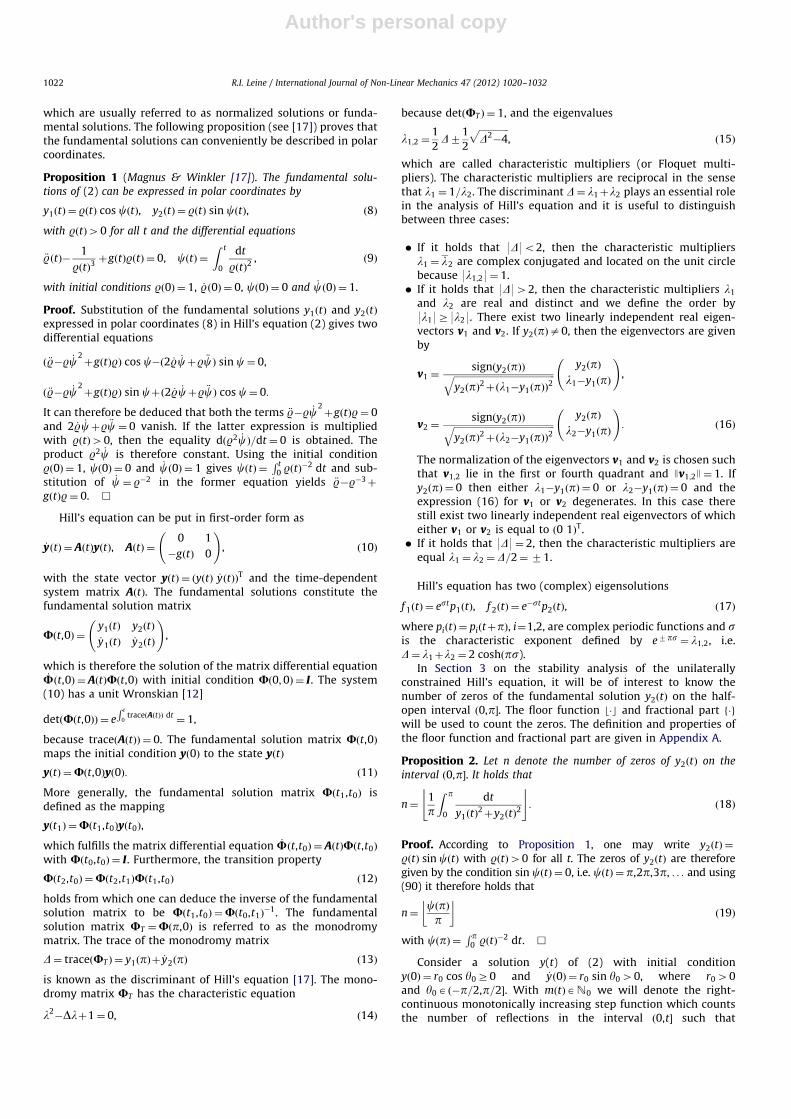
The stability of the unconstrained Mathieu equation (3)depends on the value of D, being a function of the parameters aand b. The stability boundaries in the parameter plane ða,bÞ aregiven by Dða,bÞ ¼ 72, i.e. 9y1ðpÞ9¼ 1. The unity of the determi-nant, detðUT Þ ¼ y1ðpÞ2�y2ðpÞ _y1ðpÞ ¼ 1, implies that either y2ðpÞ ¼0 and/or _y2ðpÞ ¼ 0 at a stability boundary. In other words, one candistinguish between stability boundaries for which y2ðpÞ ¼ 0 andstability boundaries for which _y2ðpÞ ¼ 0. The value of the dis-criminant Dða,bÞ and the number nða,bÞ, i.e. the number of zerosof the function y2ðtÞ on the interval ð0,p�, have been computedusing direct numerical integration on a grid of 1000�1000 pointsfor the intervals a¼�8 . . .32 and b¼ 0 . . .12. The stabilityboundaries Dða,bÞ ¼ 72 of the unconstrained Mathieu equationare depicted in Fig. 4, which is often called the Ince–Strutt

diagram. The number n changes its value in the parameter planeða,bÞ if y2ðpÞ changes sign. The boundary of the domains where n

is constant therefore agrees with those stability boundaries of theunconstrained Mathieu equation for which y2ðpÞ ¼ 0, see Fig. 5.Fig. 4 indicates the number m1 in the instability domains of theunconstrained Mathieu equation. Apparently, m1 ¼ k in the k-thinstability domain.

The stability of the equilibrium of the unilaterally constrainedMathieu equation is dependent on the number nða,bÞ and thediscriminant Dða,bÞ, which both depend on the system para-meters a and b, and the restitution coefficient e. The numericalresults for the critical restitution coefficient are depicted in Fig. 6,being the Ince–Strutt diagram for the unilaterally constrainedMathieu equation. The level curves for ec ¼ 0, 0.2, 0.4, 0.6, 0.8 and1 are shown in Fig. 6. The grey areas, being the stability domainsof the unconstrained Hill’s equation, have a critical restitutioncoefficient ec ¼ 1. It can be seen that a decrease in the restitutioncoefficient enlarges the stability domain in those regions of theparameter space for which n40, especially when n is large. Thevalue of n is zero in the so-called zeroth instability domain [30](the lower left part of Fig. 6 labeled with ec ¼ 0) and D42. Asfollows from Theorem 2, the value of the restitution coefficienthas no influence in the zeroth instability domain as the long-termbehaviour is governed by non-impacting motion. The zerothinstability domain of the unconstrained Mathieu equation istherefore also unstable for the constrained Mathieu equation.

As the stability of the constrained Mathieu equation dependson the number n and D, which characterize the unconstrainedMathieu equation, one can use common approximation methodsto investigate the stability properties of the unilaterally con-strained Mathieu equation with e¼ 0.

5.2. Averaging

A standard averaging technique [28] can be used to give anapproximation for Dða,bÞ if b=a is small. The averaging techniquecan be applied to the dynamics expressed in amplitude and phasecoordinates (polar coordinates), see for instance [21], but thistype of averaging results in an averaged system consisting of non-linear differential equations. Here, the averaging is done on the

Fig. 4. Ince–Strutt diagram and discriminant D of the unconstrained Mathieu

equation (3). In the grey stability domains holds 9D9o2. The instability domains

are white.



dynamics in comoving coordinates [27] which yields a linear setof differential equations allowing for a closed form solution of theaveraged equations.

Let o¼ 1;2,3, . . . be a resonant frequency of the Mathieuequation (3) and let b¼ Eo2 where E is a small parametermeasuring the relative intensity of the parametric excitation.Due to symmetry we know that Dða,�bÞ ¼Dða,bÞ and it thereforesuffices to consider EZ0. Furthermore, we consider the value of ato be close to resonance and set

a¼o2ð1�EdÞ, ð63Þ

where d is a detuning parameter. Following [27], comovingcoordinates z1ðtÞ and z2ðtÞ are introduced such that

yðtÞ ¼ z1ðtÞ cos otþz2ðtÞ sin ot,

_yðtÞ ¼�z1ðtÞo sin otþz2ðtÞo cos ot: ð64Þ

Differentiation of y(t) gives the relationship

_z1 cos otþ _z2 sin ot¼ 0: ð65Þ

Substitution of (64) and (65) in (3) yields the Mathieu equation incomoving coordinates:

_z1 ¼�Eoðd�2 cos 2tÞðz1 cos otþz2 sin otÞ sin ot,

_z2 ¼ Eoðd�2 cos 2tÞðz1 cos otþz2 sin otÞ cos ot: ð66Þ

The system (66) can be averaged over one period of oscillation,keeping z1 and z2 constant, i.e.

_z1 ¼�Eop

Z p

0ðd�2 cos 2tÞ cos ot sin ot dt z1

�Eop

Z p

0ðd�2 cos 2tÞ sin2ot dt z2,

_z2 ¼Eop

Z p

0ðd�2 cos 2tÞ cos2ot dt z1

þEop

Z p

0ðd�2 cos 2tÞ cos ot sin ot dt z2: ð67Þ

Consider the first resonance at o¼ 1. Evaluation of the averagedequation (67) gives

_z1 ¼�E2ð1þdÞz2,

_z2 ¼�E2ð1�dÞz1: ð68Þ

The linear planar system (68) has the general solution

z1ðtÞ ¼ c1 cosh mtþc2 sinh mt,

z2ðtÞ ¼ �

ffiffiffiffiffiffiffiffiffiffiffiffi1�d2

p1þd

ðc1 sinh mtþc2 cosh mtÞ: ð69Þ

with

m¼ E2


q: ð70Þ

In order to find an approximation for y1ðtÞ we set z1ð0Þ ¼ 1and z2ð0Þ ¼ 0 giving c1 ¼ 1, c2 ¼ 0. Hence, we obtain the approx-imation

y1ðtÞ ¼ cosh mt cos t�


p1þd

sinh mt sin t ð71Þ

for the first fundamental solution and the approximation

D¼ 2y1ðpÞ ¼�2 coshEp2


q� �ð72Þ

for the discriminant. Using E¼ b and Ed¼ 1�a for o¼ 1, we canexpress the determinant as a function of a and b

Dða,bÞ ¼�2 coshp2

ffiffiffiffiffiffiffiffiffiffiffiffiffiffiffiffiffiffiffiffiffiffiffiffib2�ð1�aÞ2

q� �: ð73Þ

Near the first resonance, it therefore holds that Do�2 if 9d9o1,or, correspondingly, if 91�a9o9b9. From (72) we calculate thelargest characteristic multiplier

l1 ¼1

2D�

1

2


p¼�cosh

Ep2


q� ��sinh

Ep2


q� �

¼�eðEp=2Þffiffiffiffiffiffiffiffiffi1�d2p

: ð74Þ

Similarly, we obtain an approximation for y2ðtÞ by setting z1ð0Þ ¼0 and z2ð0Þ ¼ 1, i.e. c1 ¼ 0 and c2 ¼�ð1þdÞ=ð


pÞ, which yields

y2ðtÞ ¼�1þdffiffiffiffiffiffiffiffiffiffiffiffi1�d2

p sinh mt cos tþcosh mt sin t: ð75Þ

Clearly, if E¼ 0, then it holds that y2ðtÞ ¼ sin t and the value of n ison the verge of turning from zero to one. Evaluation of y2ðpÞ gives

y2ðpÞ ¼1þdffiffiffiffiffiffiffiffiffiffiffiffi1�d2

p sinhEp2


q� �, ð76Þ

Fig. 6. Ince–Strutt diagram of the unilaterally constrained Mathieu equation with

critical value ec of the restitution coefficient.

Fig. 5. Diagram with the value of n of the Mathieu equation.



which is slightly larger than zero for 9d9o1. We therefore infer thatn¼0 holds around the resonance frequency o¼ 1 for small valuesof E.

The stability criterion for n¼0 and Do�2 reads as (seeTheorem 2)

eoec ¼ 9l19�1: ð77Þ

Using the approximation (74) for l1, the critical coefficient ofrestitution is approximated near the first resonance by

ec ¼ e�ðEp=2Þffiffiffiffiffiffiffiffiffi1�d2p

¼ e�ðp=2Þffiffiffiffiffiffiffiffiffiffiffiffiffiffiffiffiffib2�ð1�aÞ2

p

: ð78Þ

Inversely, for a given value of a and e one can calculate the criticalvalue of b as

bc ¼

ffiffiffiffiffiffiffiffiffiffiffiffiffiffiffiffiffiffiffiffiffiffiffiffiffiffiffiffiffiffiffiffiffiffiffiffiffiffiffiffiffiffið1�aÞ2þ 2

pln e

� �2s

ð79Þ

from which we see that a small value of the restitutioncoefficient e is beneficial for the stability of the unilaterallyconstrained Mathieu equation in the vicinity of the firstresonance.

A comparison of the approximation (79) obtained with theaveraging method and the (almost exact) numerical results isshown in Fig. 7. For a given value of ec , which has been chosen tobe 0.4, 0.6 and 0.8, the value of b has been computed using (79)and is shown as dashed lines in Fig. 7. The approximationagrees fairly well with the numerical results for ec ¼ 0:8. Signi-ficant differences can be seen for ec ¼ 0:4 and ec ¼ 0:6 becauseE¼ b can no longer considered to be small in the upper half ofFig. 7.

5.3. Approximation using Hill’s determinant

A much better approximation of the discriminant Dða,bÞ andthe critical restitution coefficient can be obtained by using Hill’sinfinite determinant as discussed in Section 4.

The function gðtÞ ¼ aþ2b cos 2t of the Mathieu equation canbe represented by gðtÞ ¼ aþbðe2itþe�2itÞ and the Fourier coeffi-cients are therefore g0 ¼ a and g1 ¼ g�1 ¼ b whereas all otherFourier coefficients are zero. The determinant Dð0Þ, see (59),therefore reads as

Dð0Þ ¼

� � � � � � � � � � � � � � � � � � � � �

� � � 1 ba�42 0 0 0 � � �

� � �b

a�22 1 ba�22 0 0 � � �

� � � 0 ba 1 b

a 0 � � �

� � � 0 0 ba�22 1 b

a�22 � � �

� � � 0 0 0 ba�42 1 � � �

� � � � � � � � � � � � � � � � � � � � �

: ð80Þ

The value of Dð0Þ can be approximated by the determinant of thecentral 5�5 block

Dð0Þ � 1�4a�32

aða�4Þða�16Þb2þ

3a�32

aða�4Þ2ða�16Þ2b4: ð81Þ

This approximation can be improved by calculating larger centralk� k blocks in (80). However, the coefficients of b2 and b4 in (81)slightly change if larger central blocks are considered. Using (61)the discriminant D can be approximated by

Dða,bÞ ¼ 2�4 sin2 1

2pffiffiffiap

� �

� 1�4a�32


3a�32

aða�4Þ2ða�16Þ2b4

!: ð82Þ

Hence, the critical restitution coefficient is determined by theequation

em1c þ

1

em1c

¼�2þ4 sin2 1

2pffiffiffiap

� �

� 1�4a�32


3a�32

aða�4Þ2ða�16Þ2b4

!, ð83Þ

or equivalently by (62). Inversely, for a given value of a and e onecan calculate an approximation of the critical value of b, based onthe terms in (82) up to order b2, as

b2c ¼

aða�4Þða�16Þ

4a�321�

em1þ2þ1

em1

4 sin2 1

2pffiffiffiap

� �0BB@

1CCA: ð84Þ

This approximation is valid (for small b) in each of the instabilitydomains but the value of m1 should be a priori known. For theMathieu equation, however, it holds that m1 ¼ k in the k-thinstability domain.

A comparison of the approximation (84) in the first instabilityregion (m1 ¼ 1) obtained with Hill’s determinant (dash-dot lines)and the approximation (79) obtained with the averaging methodand the (almost exact) numerical results is shown in Fig. 7.Clearly, the approximation (84) is much better than the approx-imation (79). However, using the averaging method one is able toestimate the value of n (and therefore m1) as a function of a and b,which cannot (easily) be done by using the method of Hill’sdeterminant.

6. Conclusions and discussion

In this paper the stability conditions of the unilaterally con-strained Hill’s equation have been addressed in detail usingFloquet theory and Lyapunov techniques. It has been shown thatthe stability of the equilibrium of the unilaterally constrainedHill’s equation depends on the discriminant D and the number n

(i.e. the number of zeros of the second fundamental solutionwithin one period) of the unconstrained Hill’s equation and on therestitution coefficient e. The remarkable simplicity of the uni-laterally constrained Hill’s equation stems from the fact that,although the system can be considered to be strongly non-lineardue to the presence of the unilateral constraint, its Poincare mapis cone-wise linear. The cone-wise linearity originates from the

Fig. 7. Approximate Ince–Strutt diagram around the first resonance by using

averaging (dashed lines) and Hill’s determinant (dash-dot lines).



homogeneity of the linear differential equation and the homo-geneity of the impact map.

The practical merit of the paper is that a precise estimation ofthe critical restitution coefficient can be obtained by calculatingthe fundamental solutions of the unconstrained Hill’s equationusing direction numerical integration methods (ODE-solvers). Inaddition, two approximation methods are proposed which giveclosed form expressions for the critical restitution coefficient: theaveraging method (Section 5.2) and the method of Hill’s infinitedeterminant (Sections 4 and 5.3). A comparison of the approx-imation techniques applied to the unilaterally constrainedMathieu equation has been given in Section 5.

The averaging method in comoving coordinates, which isemployed in Section 5.2, gives the same approximation of thecritical restitution coefficient as obtained by the averagingmethod in [21], Section 2.2.2. In [21], a two-dimensional impactevent map is constructed for the first instability domain using theaveraging method in amplitude and phase coordinates andassuming that the time difference between consecutive impactsequals tiþ1�ti ¼ pþOðEÞ. In Section 5.2, the averaging method incomoving coordinates is used to obtain an approximation of thetwo-dimensional Poincare map. This approximate Poincare mapis cone-wise linear as opposed to the approximate impact eventmap of [21] which is fully non-linear. The use of higher-orderaveraging methods to improve the approximation for largervalues of E becomes cumbersome as it takes a much larger effortand, in addition, an improved approximation for tiþ1�ti needs tobe obtained for averaging in amplitude and phase coordinates.

The approximation of the critical restitution coefficient usingHill’s infinite determinant, see Sections 4 and 5.3, is very accurateand can easily be improved by considering larger central blocks forthe determinant Dð0Þ. However, the method using Hill’s infinitedeterminant gives no direct way to determine the number n.

The analysis has shown that the impact time instants aredefined by the zero-crossings of the solution of the unconstrainedHill’s equation, which are always separated in time. Accumulationpoints of impacts can therefore not exist in the unilaterallyconstrained Hill’s equation (4) as has been proven in Theorem 1.If, however, the location of the constraint is moved to a non-zero position, which does not agree with the equilibrium of theunconstrained system, i.e. xðtÞZxc 40, then accumulation pointsare possible. The unilaterally constrained Hill’s equation withxc 40 does not have an equilibrium and the contact force l in Eq.(5) does not vanish. The framework of non-smooth dynamics istherefore needed to describe and understand the dynamics of theunilaterally constrained Hill’s equation with non-zero constraintposition. Moreover, the non-linear dynamics becomes far morecomplicated because the homogeneity of the impact conditions(27), and also the cone-wise linearity of the Poincare map, is lost.

The present paper gives more insight in the stability properties ofHill’s equation with unilateral constraint, being an archetype of aparametrically excited non-smooth dynamical system with impulsivemotion. Further research will focus on the application and extensionof the obtained results to the stability analysis of multi-degree-of-freedom autoparametric systems with unilateral constraints.

Appendix A. Floor function and fractional part

Definition 1 (Floor function and fractional part). With bxc wedenote the floor function defined by

bxc ¼ fmax kAZ9krxg ð85Þ

and with fxg the fractional part defined by

fxg ¼ x�bxc: ð86Þ

The fractional part can be expressed in trigonometric functions as

fxg ¼1

2�

1

parctanðcotðpxÞÞ, ð87Þ

where cotðpkÞ ¼ þ1 for kAZ. The floor function has the follow-ing property:

bxcþbycrbxþycrbxcþbycþ1, ð88Þ

and the equality bxcþbyc ¼ bxþyc holds only if fxgþfygo1, orusing (87), if cotðpxÞþcotðpyÞ40. More precisely, the relations(88) can be formulated as

bxþyc ¼bxcþbyc if cotðpxÞþcotðpyÞ40,

bxcþbycþ1 if cotðpxÞþcotðpyÞr0:

(ð89Þ

The floor function can be used to count the number of zeros ofsinusoidal functions. The function f 1ðxÞ ¼ sinðxÞ has the zeros kpwith kAZ and the number of zeros on the interval ð0,a� thereforeamounts to

m1 ¼a

p

j k: ð90Þ

The function f 2ðxÞ ¼ sinðxþbÞ has the number of zeros

m2 ¼aþb

p

� ��

b

p

� �, ð91Þ

which, using (89), can be expressed as

m2 ¼m1 if cotðaÞþcotðbÞ40,

m1þ1 if cotðaÞþcotðbÞr0:

(ð92Þ

References

[1] M.V. Bartuccelli, J.H.B. Deane, G. Gentile, S.A. Gourley, Global attraction to theorigin in a parametrically driven nonlinear oscillator, Applied Mathematicsand Computation 153 (1) (2004) 1–11.

[2] M.V. Bartuccelli, G. Gentile, K.V. Georgiou, On the stability of the upside-down pendulum with damping, Proceedings of the Royal Society A: Mathe-matical, Physical and Engineering Sciences 458 (2018) (2002) 255–269.

[3] T. Birkandan, M. Hortac-su, Examples of Heun and Mathieu functions assolutions of wave equations in curved spaces, Journal of Physics A: Mathe-matical and Theoretical 40 (2007) 1105–1116.

[4] H.W. Broer, I. Hoveijn, M. Van Noort, C. Simo, G. Vegter, The parametricallyforced pendulum: a case study in 1 1

2 degree of freedom, Journal of Dynamicsand Differential Equations 16 (4) (2004) 897–947.

[5] H.W. Broer, I. Hoveijn, M. Van Noort, G. Vegter, The inverted pendulum: asingularity theory approach, Journal of Dynamics and Differential Equations157 (1) (1999) 120–149.

[6] H.W. Broer, M. Levi, Geometrical aspects of stability theory for Hill’sequations, Archive for Rational Mechanics and Analysis 131 (1995) 225–240.

[7] B. Brogliato, Absolute stability and the Lagrange–Dirichlet theorem with mono-tone multivalued mappings, Systems & Control Letters 51 (2004) 343–353.

[8] M. Cartmell (Ed.), Introduction to Linear, Parametric and Nonlinear Vibra-tions, Chapman and Hall, London, 1990.

[9] B.J. Daiuto, T.T. Hartley, S.P. Chicatelli, The Hyperbolic Map and Applicationsto the Linear Quadratic Regulator, Lecture Notes in Control and InformationSciences, vol. 110, Springer, Berlin, 1989.

[10] Ch. Glocker, Set-Valued Force Laws, Dynamics of Non-Smooth Systems,Lecture Notes in Applied Mechanics, vol. 1, Springer-Verlag, Berlin, 2001.

[11] A.P. Ivanov, The stability of mechanical systems subjected to impulsive actions,Journal of Applied Mathematics and Mechanics 65 (4) (2001) 617–629.

[12] D.W. Jordan, P. Smith, Nonlinear Ordinary Differential Equations, OxfordUniversity Press, New York, 2007.

[13] J.P. LaSalle, The Stability and Control of Discrete Processes, Applied Mathe-matics Sciences, vol. 62, Springer, New York, 1961.

[14] R.I. Leine, T.F. Heimsch, Global uniform symptotic attractive stability of thenon-autonomous bouncing ball system, Physica D (2011), http://dx.doi.org/10.1016/j.physd.2011.04.013.

[15] R.I. Leine, H. Nijmeijer, Dynamics and Bifurcations of Non-Smooth Mechan-ical Systems, Lecture Notes in Applied and Computational Mechanics, vol. 18,Springer Verlag, Berlin, 2004.



[16] R.I. Leine, N. van de Wouw, Stability and Convergence of Mechanical Systems,with Unilateral Constraints, Lecture Notes in Applied and ComputationalMechanics, vol. 36, Springer Verlag, Berlin, 2008.

[17] W. Magnus, S. Winkler, Hill’s Equation, Dover Publications, New York, 1979.[18] A.H. Nayfeh, D.T. Mook, Nonlinear Oscillations, Wiley-Interscience, Chichester,

1979.[19] W. Paul, Electromagnetic traps for charged and neutral particles, Reviews of

Modern Physics 62 (1990) 531–540.[20] F. Pellicano, A. Fregolent, A. Bertuzzi, F. Vestroni, Primary and parametric

non-linear resonances of a power transmission belt: experimental andtheoretical analysis, Journal of Sound and Vibration 244 (4) (2001) 669–684.

[21] D.D. Quinn, The dynamics of two parametrically excited pendula with impacts,International Journal of Bifurcations and Chaos 15 (6) (2005) 1975–1988.

[22] S.W. Shaw, R.H. Rand, The transition to chaos in a simple mechanical system,International Journal of Nonlinear Mechanics 24 (1) (1989) 41–56.

[23] A. Tondl, Quenching of Self-Excited Vibrations, Elsevier, Amsterdam, 1991.

[24] A. Tondl, T. Ruijgrok, F. Verhulst, R. Nabergoj, Autoparametric Resonance inMechanical Systems, Cambridge University Press, New York, 2000.

[25] S.R. Valluri, R. Biggs, W. Harper, C. Wilson, The significance of the Mathieu–

Hill differential equation for Newton’s apsidal precession theorem, CanadianJournal of Physics 77 (5) (1999) 393–407.

[26] M. van Noort, The Parametrically Forced Pendulum, A Case Study in 1 12 Degree

of Freedom, Ph.D. thesis, Rijksuniversiteit Groningen, The Netherlands, 2001.[27] F. Verhulst, Nonlinear Differential Equations and Dynamical Systems, Springer,

Berlin, 1996.[28] F. Verhulst, Parametric and auto-parametric resonance, Acta Applicandae

Mathematicae 70 (2002) 231–264.[29] E.T. Whittaker, G.N. Watson, A Course of Modern Analysis, Cambridge

University Press, Cambridge, 1927.[30] V.A. Yakubovich, V.M. Starzhinskii, Linear Differential Equations with Periodic

Coefficients 1 and 2, Wiley, New York, 1975.


(This is a sample cover image for this issue. The actual ... vertically forced pendulum or the...

Documents

Transcript of (This is a sample cover image for this issue. The actual ... vertically forced pendulum or the...