This document gives a detailed summary of the new features...
146
This document gives a detailed summary of the new features and improvements of FEM-Design version 17. We hope you will enjoy using the program and its new tools and possibilities. We wish you success. StruSoft, Developer Team StruSoft AB www.strusoft.com May 4th, 2018
Transcript of This document gives a detailed summary of the new features...

This document gives a detailed summary of the new features and improvements of FEM-Design version
17.
We hope you will enjoy using the program and its new tools and possibilities. We wish you success.
StruSoft,
Developer Team
StruSoft AB www.strusoft.com May 4th, 2018

2
Legend
Pay attention / Note
Useful hint
Example
Clicking left mouse button
Clicking right mouse button
Clicking middle mouse button

3
What is new in FEM-Design 17?
The list of all new major features and improvements is following:
- Correct model tool
- Plastic calculation of trusses, supports and connections
- Post-tensioned cable
- Fire design for steel bars
- Pile
- Composite sections for beams, columns and piles
- Wall buckling
- Properties dialogs available from the quick menu
- Joint stiffness calculation
- Displaying relevant load combination for max. of combinations results
- Fully rigid diaphragm
- Colour palette for displacement-like results in 3D modules
- New tables to list and new listing options
- Wall corbel
- Joint library and many more improvements of steel joints
- Notional load
- Manual position numbering
- Improved documentation module
What is new in FEM-Design 17.1?
- Construction stages (Phase 1)
- Improved storey management
- Run Script
- Option to hide extra information in the numeric results

4
Table of contents
1. TOOLS ............................................................................................................................................. 7
1.1. CORRECT MODEL ................................................................................................................................ 7
1.2. SCRIPTING ....................................................................................................................................... 24
1.3. POSITION NUMBERING TOOL............................................................................................................... 25
1.4. SECTION LIST .................................................................................................................................... 28
1.5. LOAD COMBINATION ANALYSIS SETUP LIST ............................................................................................. 30
1.6. ARRANGING TABLES WHEN LISTING TO EXCEL ........................................................................................ 31
1.7. “FILL ALL CELLS” OPTION FOR LISTING TABLES ........................................................................................ 31
1.8. DISPLAYING NAME OF LOAD CASE/COMBINATION FOR LOAD CASE/COMBINATION RESULT TABLES .................. 32
1.9. GET GUID (GLOBALLY UNIQUE IDENTIFIER) .......................................................................................... 33
2. USER INTERFACE ........................................................................................................................... 35
2.1. PROPERTIES DIALOG AVAILABLE FROM QUICK MENU FOR OBJECTS ............................................................. 35
2.2. DIFFERENT MODES TO DISPLAY STOREYS ............................................................................................... 36
2.3. VISUALISATION OF EDGE CONNECTION IS IMPROVED ............................................................................... 37
2.4. RESTORE VIEW RETURNING TO INPUT ................................................................................................... 38
2.5. LEADING LINE FOR NUMERIC VALUES AND LABELS ................................................................................... 39
2.6. ALIGN REGION TO PLANE .................................................................................................................... 41
2.7. VERTICAL DIMENSION LINES ................................................................................................................ 41
2.8. PHYSICAL VIEW ................................................................................................................................. 42
2.9. PHYSICAL ALIGNMENT FOR INTERMEDIATE SECTION ................................................................................ 43
2.10. BLINKING LAYERS .............................................................................................................................. 43
3. STRUCTURE ................................................................................................................................... 45
3.1. IMPROVED STOREY DIALOG ................................................................................................................. 45
3.2. REFERENCE PLANE ............................................................................................................................. 45
3.3. COMPOSITE SECTIONS ....................................................................................................................... 47
3.4. PILE ................................................................................................................................................ 48
3.5. HORIZONTAL BEDDING MODULI OF FOUNDATION SLAB ............................................................................ 57
3.6. CAMBER SIMULATION OPTION FOR BEAMS AND PROFILED PLATES ............................................................. 58
3.7. EASIER DEFINITION OF COLUMN CORBEL’S LOAD POSITION ....................................................................... 59
3.8. POST-TENSIONED CABLE..................................................................................................................... 60
3.8.1. General ........................................................................................................................................ 60
3.8.2. Layout wizard .............................................................................................................................. 75
3.9. “NO SHEAR” EDGE MACRO FOR PLANE WALLS ....................................................................................... 76
3.10. WALL CORBEL .................................................................................................................................. 77
3.11. EDITABLE SURFACE CONNECTION (SOIL) ................................................................................................ 79
4. LOAD ............................................................................................................................................. 80
4.1. CONSTRUCTION STAGES ..................................................................................................................... 80
4.2. PRE DEFINED PSI VALUES FOR TEMPORARY LOAD GROUPS ........................................................................ 86
4.3. IGNORED TEMPORARY LOAD CASES ...................................................................................................... 86
4.4. DEVIATION LOAD IMPROVED ............................................................................................................... 86
5
4.5. NOTIONAL LOAD ............................................................................................................................... 88
4.6. LOAD COMMENTS ............................................................................................................................. 90
4.7. LOAD EXPORT / IMPORT VIA CLIPBOARD ................................................................................................ 91
5. ANALYSIS ....................................................................................................................................... 92
5.1. PLASTIC TRUSSES, SUPPORTS AND CONNECTIONS .................................................................................... 92
5.2. MODIFIED BEHAVIOUR OF TRUSSES IN NON-LINEAR ELASTIC (NLE) AND NON-LINEAR ELASTIC + PLASTIC (PL)
CALCULATIONS ................................................................................................................................. 93
5.3. CHECK FOR IDENTICAL COPIES OF STRUCTURAL OBJECTS AND LOADS .......................................................... 95
5.4. FULLY RIGID DIAPHRAGM ................................................................................................................... 96
5.5. SELECTING ALL RELEVANT SHAPES IN MODAL ANALYSIS ........................................................................... 97
6. RC DESIGN ..................................................................................................................................... 98
6.1. RC BAR DETAILED RESULT REINFORCEMENT EXPORT TO DWG/DXF .......................................................... 98
6.2. RC BAR DETAILED RESULT DRAWING IMPROVEMENTS ............................................................................. 99
6.3. RC SHELL BUCKLING ........................................................................................................................ 100
6.4. RC SHELL – EN 1992-1-1, ANNEX F ................................................................................................. 104
7. STEEL DESIGN .............................................................................................................................. 106
7.1. FIRE DESIGN ................................................................................................................................... 106
7.2. STEEL JOINT STIFFNESS ..................................................................................................................... 111
7.3. COLUMN BASE JOINT CONCRETE TENSION FAILURES .............................................................................. 114
7.4. “ROTATED” OPTION FOR HOLLOW SECTIONS ....................................................................................... 119
7.5. JOINT LIBRARY ................................................................................................................................ 120
7.6. STEEL JOINTS ADDED TO FILTER ......................................................................................................... 123
7.7. USER INTERFACE IMPROVEMENTS IN STEEL JOINTS MODULE ................................................................... 123
7.7.1. Tooltip for joint bars ................................................................................................................. 123
7.7.2. Joint bar display option ............................................................................................................. 124
7.7.3. Navigation buttons for steel joints ............................................................................................ 124
7.8. STEEL JOINT UTILIZATION IN DOCUMENTATION .................................................................................... 125
8. RESULTS ...................................................................................................................................... 125
8.1. DOMINANT LOAD COMBINATION SHOWN ON RESULTS FOR MAXIMUM OF LOAD COMBINATIONS .................. 125
8.2. DISPLACEMENT-LIKE RESULTS IMPROVED ............................................................................................ 125
8.3. SHEAR CENTER RESULT ..................................................................................................................... 129
8.4. MASS RESULT ................................................................................................................................. 131
8.5. MINIMUM AND MAXIMUM VALUES OF SOIL RESULTS IN COLOUR PALETTE VIEW ......................................... 133
8.6. LOCAL STABILITY RESULTS WITH MORE DETAILS .................................................................................... 134
8.7. COLOURS OF PRINCIPAL STRESSES, MOMENTS AND NORMAL FORCES ....................................................... 134
8.8. OPTION TO HIDE FINITE ELEMENTS FOR COLOUR PALETTE RESULTS ........................................................... 137
8.9. SCALE TO VIEW OPTION FOR COLOUR PALETTE RESULTS ......................................................................... 138
9. DOCUMENTATION ...................................................................................................................... 139
9.1. OPTION TO HIDE SECTIONS ............................................................................................................... 139
9.2. APPEND TEMPLATES ........................................................................................................................ 139
9.3. DOCGRAPH WINDOWS ARE CREATED ACCORDING TO THE SAVED WINDOW SETTINGS ................................. 140

6
10. OTHERS ....................................................................................................................................... 142
10.1. FEM-DESIGN CENTER ..................................................................................................................... 142
10.2. DRAG AND DROP ............................................................................................................................ 143
10.3. FEM-DESIGN SUPPORT TOOL ........................................................................................................... 144
10.4. COMPANY SETTINGS ........................................................................................................................ 145
10.5. GRAPHIC ENGINE SETTINGS AND DRAFT MODE ..................................................................................... 146
10.6. TIMESAVE ...................................................................................................................................... 146

7
1. Tools
1.1. Correct model
Correct model tool is a revolutionary function to fix the models having geometrical errors, in semi-
automatic way, with supervision of the user. This tool helps to fix the following types of errors in the
model:
- object multiplication and overlap
- geometrically incorrect objects (very small region parts, very small angles, divided region edges,
etc.)
- incorrectly positioned objects
Correct model tool is the replacement of Object merge (in earlier versions), which is no more available in
version 17. Correct model tool is a semi-automatic system which necessarily needs user-interaction.
It draws attention to the possible errors of the model and in most cases also offers solution(s), but the
User has to decide whether it is really an error or not, and if it is, how to fix it.
Correct model can be launched from Tools/Correct model or from the toolbar ( ).
After launching Correct model, User needs to select the elements to be checked.

8
Then in the pop-up dialog, task(s) should be selected. Using the buttons Select all and Clear all, all
correction tasks can be selected or cleared in one click.
After pressing Start, the correcting process begins. It runs row by row and the current step turns green.
The view is focused on the incorrect object (part).
Fix object multiplication and overlap
Fix geometrically incorrect objects
Fit objects to storeys, axes and reference planes
Fit objects to each other
9
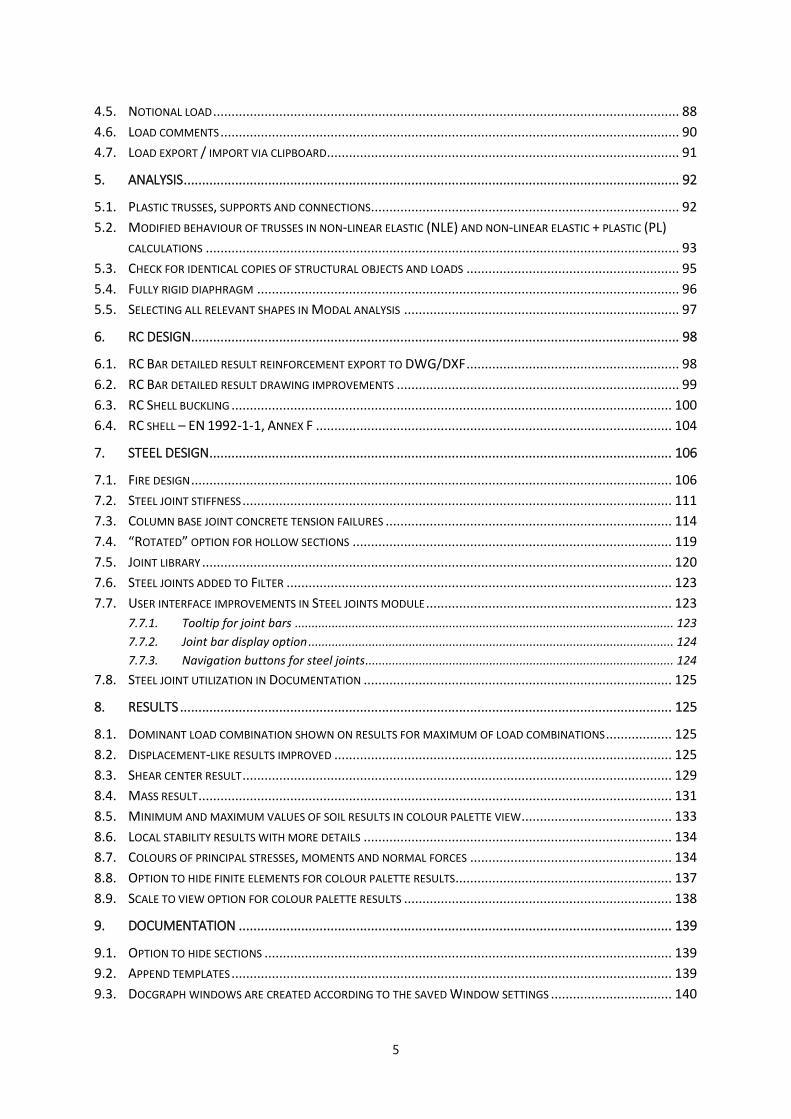
The table below contains the meaning of the flashing red object depending on the current correction
task:
Correction task (type) What is flashing?
Delete identical copies object to be deleted
Fix overlap current object and its modified version
are both flashing
Chamfer sharp angles the part of the region to be removed
Fix small areas and lines the part of the line/region to be removed
Merge region lines the region line to be merged
Fixing geometrically incorrect objects the object to be fixed
Fit objects to storeys, axes and reference planes the suggested new position of the
incorrectly placed object Fit objects to each other
In order to decide what to do with each object, the User has the following choices:
- Ignore: the object will not be modified
- Mark: the object will be marked according to the colour and text set in the Marker dialog
- Fix: the object will be deleted/modified according to the program’s suggestion. The number
in the table in Fixed cell of the current correction task’s row is increased by one. The fixed
object turns into green.

10
Ignore all, Mark all, Fix all acts on all further incorrect objects found by the current correction task
(highlighted by green in the table).
After one of the abovementioned buttons is pressed, the next incorrect object – if exists – gets into focus
and is highlighted
Show again focuses on the current objects. It can be useful if the User gets lost in a large model.
Break cancels the correction process but the previously performed modifications are kept.
Once the correction process is finished (or cancelled) the modifications can be applied to the model by
pressing either Apply or OK. In case of OK the dialog closes. All modifications can be discarded by
pressing Reset if they were not yet applied on the model.
Settings commands let the user save/load the selected correction tasks and their tolerances. A small
but quite complex example at the end of this chapter shows in detail how to use Correct model tool.
Using Auto button and applying its modification on the model is not recommended, because in practice
in most cases there is no exact solution:
- fixing an error may generate or eliminate other problems
- fixing the same error in different ways may generate/eliminate different problems
- consequently, the correcting process can be iterative
However, Auto is useful to get an estimation of errors and their type in the model.
See detailed description of each correction task as follows.

11
Delete identical copies
If more identical element exists in the same position, it deletes all
identical copies, and counts as one correction in the Fixed column on
the Correct model dialog.
This is not working for intermediate sections, post-tensioned cables and corbels.
Fix overlaps
It fixes overlapping regions and lines. Existing objects can be shrunk
or erased, but function will not generate new objects (e.g. a region
can not fall apart).
Overlapping is allowed for the Loads.
This is not working for isolated and wall foundations’ regions and corbels.
Sharp angles
Sharp corners under 10° will be fixed according to the given tolerance. The
highlighted part of object will be removed. If an element has smaller
dimension than the given tolerance, the whole element will be removed.
Fix small areas and lines
Objects within the tolerance range will be removed. It will fix small holes,
long narrow areas etc.
Merge region lines
Merge region lines function merges two lines/curves of a region into one
line/curve if they are in the range of tolerance. Too flat curves may be
replaced by line. The figure below shows examples how the tolerance is
measured.
Align to structural grid

12
This function aligns objects to structural grids (axes, storeys or reference planes). Alignment is done by
orthogonal projection of object’s checkpoints to the structural grid within the tolerance. The check-
points are shown below for line, arc and circle:
Once an object is placed on a grid by Correct model tool, it will not be detached from it
by any next correction step.
Correct model tool does not check structural grid for possible errors, like axes too close
to each other or not perfectly parallel.
Stretch to structural grid
This function will stretch regions and lines to the intersection of axes
within given tolerance.
If the geometry of the object is incorrect (e.g. shell is not laying in plane) this function
cannot be performed.
Align regions
It aligns a region (projection) to other region’s plane that is within the
given tolerance both in direction perpendicular to and parallel with the
region’s plane.
Stretch to crossing regions
This function will stretch objects to the crossing regions within given
tolerance.

13
Stretch regions in plane
Regions laying in same plane will be stretched to each other within
given tolerance.
Stretch regions in plane
Lines laying within given tolerance to other objects will be stretched.
Align points
Points (objects) will be aligned to closest object within tolerance.
Restrictions
- Correct model cannot handle:
• peak smoothing regions
• connections (point, line, surface)
• bar, shell components
• building cover
• it doesn’t work in Analysis and Design tabs
- Only the visible objects can be modified.
- Columns and walls need to be vertical and will stay vertical after the modifications
as well.
- Isolated, wall foundation and foundation slab need to be and remain horizontal.
- Pile can be placed in any direction, but cannot be horizontal.
- Corbel is not handled by Correct model and cannot be used as an object to fit
other objects to.
Correct model works in multiple-window mode as well.
Example

14
The following example shows the process of fixing geometrical errors of a small model with different
types of errors:
The example file can be downloaded from here.
Let’s launch Correct model tool. Select all structural elements by Ctrl+A (or box), then all correction tasks
in the dialog by clicking on Select all. To get a quick overview of what kind of problems occur in the
model, just click on Auto button.

15
The process searches for all errors and fixes them in a way that most probably is not always the way that
the user intends to fix them However, this way User can get a good estimation on the type and amount
of errors (by looking at the values in the Fixed column).
So, in this case, all together about 15 errors should be fixed.
Now click on Reset to discard all modifications done by the automatic process.
Now click on Start to see and decide about all the errors one by one.

16
The doubled support in the bottom left corner is found first. Now click on Fix to eliminate it.
The number in the Fixed column of “Delete identical copies” task is set to 1.
Overlap of the large plate and the small plate over the column is found as next error. The large plate is
blinking, so by clicking on Fix, that one would be modified. However, we know that it is the small region
that is incorrect, so this time let’s click on Ignore instead.

17
Now the small plate is blinking, so by clicking on Fix, it is modified and fit into the large plate.
The corrected small plate is displayed in green contour. The number in the Fixed column of “Fix overlaps”
task is set to 1.

18
The next problem is found by “Fix small areas and lines” task: a very small region part. Let’s remove it by
clicking on Fix.
The removed small region part is displayed by dashed line, and number of fixed objects for “Fix small
areas and lines” task is set to 1.
The next problem, a very small hole is highlighted. We decide not to delete it but deal with it later, so
let’s mark it. First let’s click on the Marker and set the marking text, colour and font type. After clicking
OK in the Marker dialog, let’s click on the Mark.
19
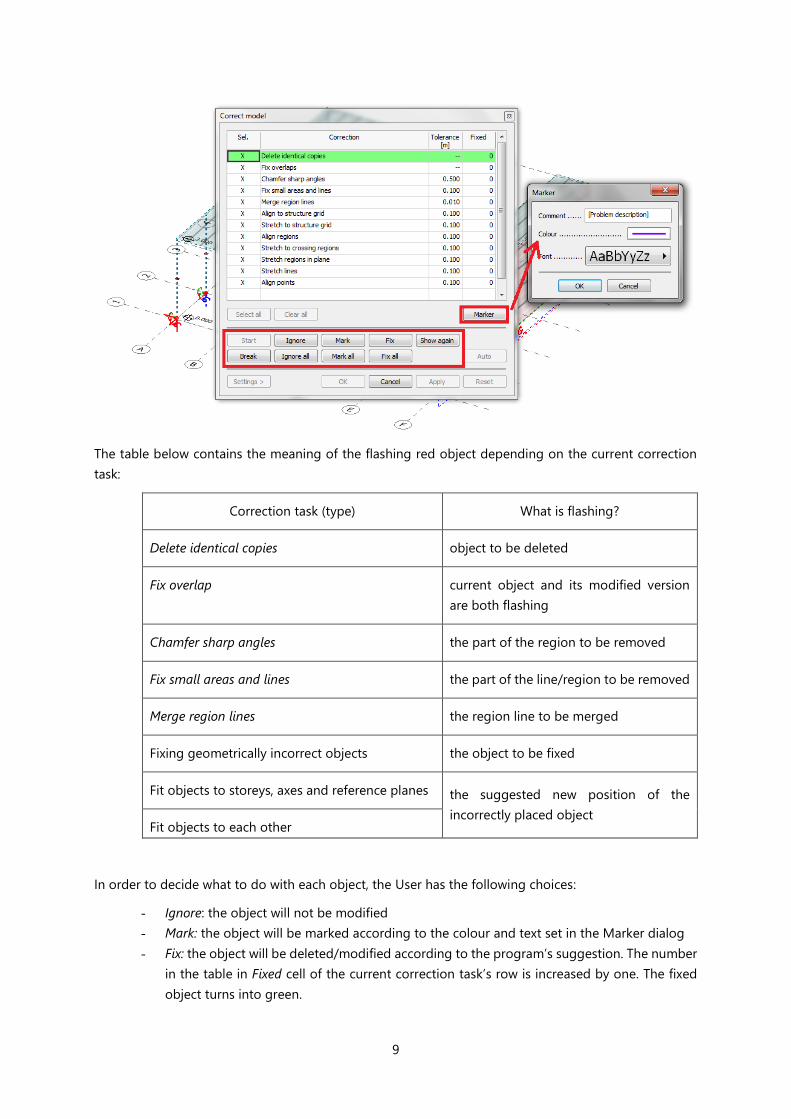
The wall with very small hole will be marked for later investigation.
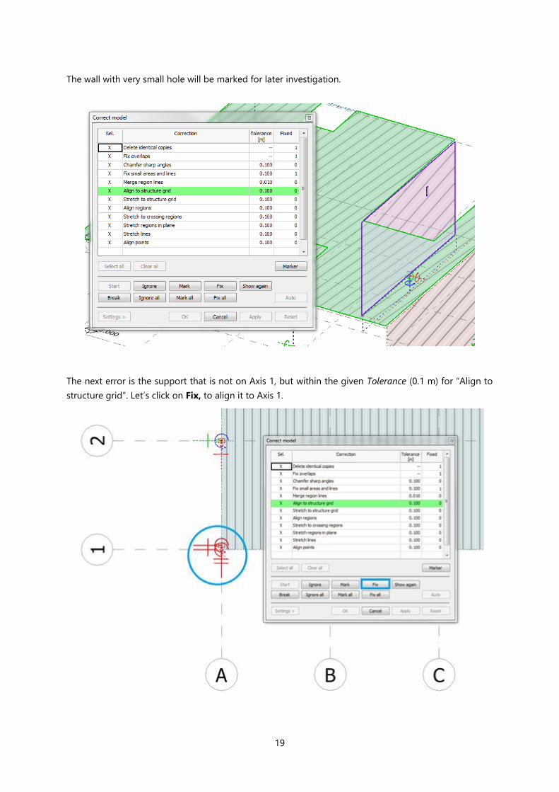
The next error is the support that is not on Axis 1, but within the given Tolerance (0.1 m) for “Align to
structure grid”. Let’s click on Fix, to align it to Axis 1.

20
The number in the Fixed column of “Align to structure grid” task is set to 1. The corrected support is
green on the next picture. The next misplaced object - the column, above it - is blinking. Let’s fix it too.
The number in the Fixed column of “Align to structure grid” task is increased to 2. The corrected column
is green on the next picture, and the next misplaced object - the large plate - is blinking (since it is
slightly above Storey 1). Let’s fix it as well and do the same for the next blinking small plate.
Finally, four objects are fixed by “Align to structure grid” task (one support, one column and two plates)
and the next incorrect object is the line support that is just a bit short to reach to Axis 1. Let’s click Fix
to stretch it to Axis 1.

21
The number for the Fixed objects in the “Stretch to structure grid” task is set to 1. The next object to be
fixed is the wall above the previously fixed line support, which is also too short to reach Axis 1. Let’s click
Fix to stretch it, too.
The next error is found by the “Stretch to crossing regions” task: the plate edge does not fit to the wall
below.

22
Then “Stretch lines” task finds a line support that is not connected to the wall above it. Let’s click on Fix
to move it under the wall.
The next incorrect object is a column that is not exactly above the point support. But we decide that the
column is at the right place, so click Ignore to skip it.
23
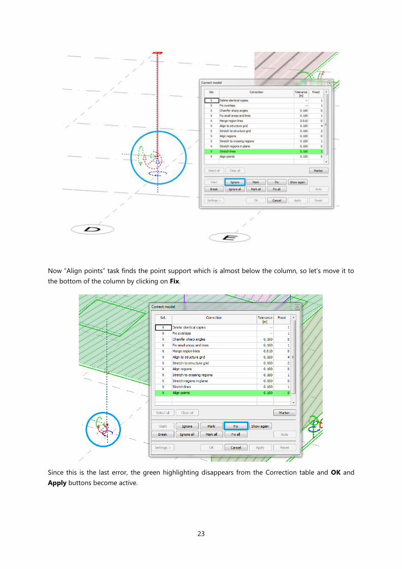
Now “Align points” task finds the point support which is almost below the column, so let’s move it to
the bottom of the column by clicking on Fix.
Since this is the last error, the green highlighting disappears from the Correction table and OK and
Apply buttons become active.

24
By clicking on OK, the corrections will be applied to the model. The objects that were marked in the
dialog are displayed with the marker text.
1.2. Scripting
We support a basic automation workflow through scripting. It is capable to load/save file, execute
analysis calculation and create outputs as .csv list or .docx documentation. With that you can batch-
analyze models created in other programs or directly in .struxml. Or execute long calculations during the
night.
The script commands approximate the usual interface, as if you filled inputs on the dialog and press the
OK button. So for the meaning of the parameters look at the corresponding panel in the UI.
25
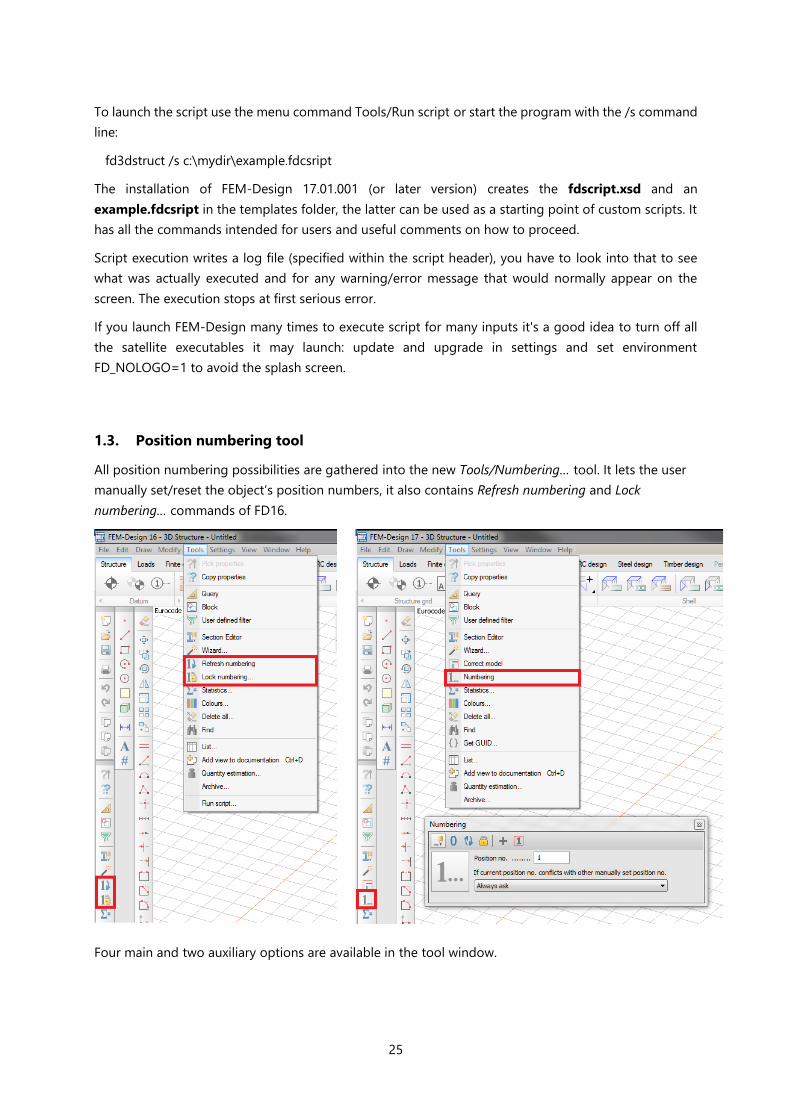
To launch the script use the menu command Tools/Run script or start the program with the /s command
line:
fd3dstruct /s c:\mydir\example.fdcsript
The installation of FEM-Design 17.01.001 (or later version) creates the fdscript.xsd and an
example.fdcsript in the templates folder, the latter can be used as a starting point of custom scripts. It
has all the commands intended for users and useful comments on how to proceed.
Script execution writes a log file (specified within the script header), you have to look into that to see
what was actually executed and for any warning/error message that would normally appear on the
screen. The execution stops at first serious error.
If you launch FEM-Design many times to execute script for many inputs it's a good idea to turn off all
the satellite executables it may launch: update and upgrade in settings and set environment
FD_NOLOGO=1 to avoid the splash screen.
1.3. Position numbering tool
All position numbering possibilities are gathered into the new Tools/Numbering… tool. It lets the user
manually set/reset the object’s position numbers, it also contains Refresh numbering and Lock
numbering… commands of FD16.
Four main and two auxiliary options are available in the tool window.

26
Manual position numbering
1. type required position number into the Position no. textbox
2. select option for handling position number conflict
3. select object(s) to set position number for
In case more objects are selected, the first one gets the position number typed by the user
and for the next ones it is increased automatically.
To set position number of component objects, like edge connections, corbels, post-tensioned cables,
punching regions, the Select component (…) auxiliary option has to be checked.
Objects with manually set position number can be highlighted by checking the last option of the tool
window.
27
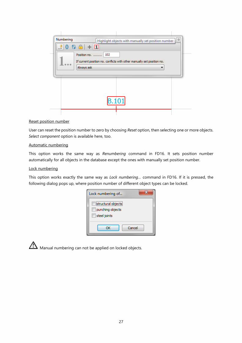
Reset position number
User can reset the position number to zero by choosing Reset option, then selecting one or more objects.
Select component option is available here, too.
Automatic numbering
This option works the same way as Renumbering command in FD16. It sets position number
automatically for all objects in the database except the ones with manually set position number.
Lock numbering
This option works exactly the same way as Lock numbering… command in FD16. If it is pressed, the
following dialog pops up, where position number of different object types can be locked.
Manual numbering can not be applied on locked objects.

28
1.4. Section list
A new type of table – Sections – can be listed. It contains all sectional data (width, height, area, inertias,
etc.)
In the List tables dialog select Tables/ Structures/ Sections, then click on the List table button.
In the generated Section table, the last column – Other - contains the detailed dimensions of the section.
Currently it is filled only for RHS, I and composite sections.
3
2
1

29
30
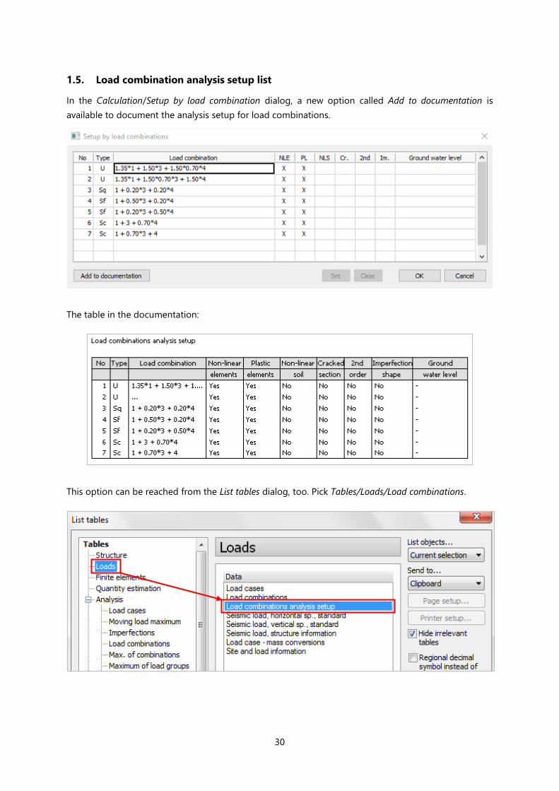
1.5. Load combination analysis setup list
In the Calculation/Setup by load combination dialog, a new option called Add to documentation is
available to document the analysis setup for load combinations.
The table in the documentation:
This option can be reached from the List tables dialog, too. Pick Tables/Loads/Load combinations.

31
1.6. Arranging tables when listing to Excel
New options have been implemented into the feature List to Excel. From now on User can choose, if the
tables should be placed into different Excel-worksheets or into the same worksheet under or next to
each other.
1.7. “Fill all cells” option for listing tables
In order to ease sorting data in Excel after exporting tables, User can fill the empty cells by turning on
the “Fill all table cells” option. This option is also available in the Documentation, in the Table properties
dialog in the Option tab.
The left part of table on figure below shows the result if the checkbox is off, and right part shows when
it is on.

32
1.8. Displaying name of load case/combination for load case/combination result
tables
In FD 17 the name of the load combinations and load cases can be displayed for the load case and load
combination result tables.
Check Show hidden columns checkbox in Table properties dialog:
1.

33
1.9. Get GUID (Globally Unique Identifier)
The Get GUID function enables the query of the GUID of elements. This can be useful for identification
of structural objects imported/exported via Struxml.
The function-button can be found in the Tools menu, but it is not on the Toolbar ( ) by default.User
can put it there by using Customize… command which is available by right clicking on the toolbar.
2.

34
After launching Get GUID, pick the element(s). The pop-up window shows the Globally Unique Identifiers
of selected element(s). They can be sent to the clipboard by clicking on “Send to clipboard” button.
GUIDs for analytical and physical model of a bar are different.
Analytical view:
Physical view:
If the bar is saved in struxml format, these GUIDs can be found there as well.

35
2. User interface
2.1. Properties dialog available from Quick menu for objects
Simply select any object by right click, or more objects of the same type by box selection, then click
“Properties ” in the Quick menu to check/modify its/their properties. This function works for structural
objects, loads or design elements.
Objects that are part of other object (e.g. edge connections, corbels, reinforcement regions, etc.)usually
can be selected by left-to-right (blue) box selection only, because right clicking always selects the main
object (shell, bar).

36
2.2. Different modes to display storeys
In Settings/Display/Storey dialog User can choose from three options for the appearance of the given
storey.
All objects that are in the plane of the storey, or crossing the storey above or below according to the
selected setting, are displayed
The pictures below show the whole structure and how it is displayed according to the selected option.
37
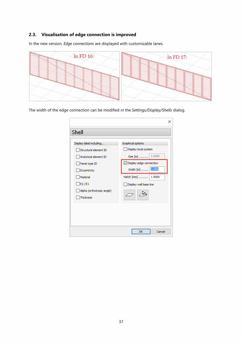
2.3. Visualisation of edge connection is improved
In the new version, Edge connections are displayed with customizable lanes.
The width of the edge connection can be modified in the Settings/Display/Shells dialog.

38
2.4. Restore view returning to input
Once a view set in an input tab gets modified in the Analysis or in a design tab, User can return into an
input tab while automatically restoring the original view. See an example in the following figures.
Using Ctrl:
Input tabs Analysis and design tabs
CTRL +
1.
3.
2.
Original view New view in RC design
Back to original view

39
Without pressing Ctrl the view doesn’t switch back:
2.5. Leading line for numeric values and labels
If a numeric value or a label is moved away from the referred point, a thin leading line appears.
1.
3.
2.
Original view New view in RC design
Back to original view

40

41
2.6. Align region to plane
This function will align regions to selected plane in any direction with two clicks. The feature can be
found in Modify/Modify region.
Click the icon , select regions to be aligned, and then select the reference plane.
All selected object will be projected to the reference plane.
2.7. Vertical dimension lines
From now vertical dimension lines can be placed without modifying the user coordinate-system.
In the Dimensioning dialog select the parallel direction with global Z axis or with z axis of UCS.

42
2.8. Physical view
In FEM-Design 17 the analytical and physical view of an object is clearly separated. The physical view
shows the real position of the physical element, while the analytical view shows the calculation model.
Analytical Physical
Analytical Physical
43
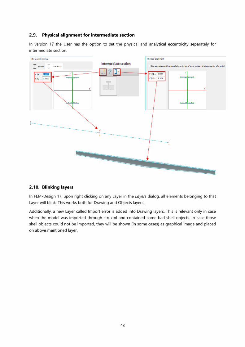
2.9. Physical alignment for intermediate section
In version 17 the User has the option to set the physical and analytical eccentricity separately for
intermediate section.
2.10. Blinking layers
In FEM-Design 17, upon right clicking on any Layer in the Layers dialog, all elements belonging to that
Layer will blink. This works both for Drawing and Objects layers.
Additionally, a new Layer called Import error is added into Drawing layers. This is relevant only in case
when the model was imported through struxml and contained some bad shell objects. In case those
shell objects could not be imported, they will be shown (in some cases) as graphical image and placed
on above mentioned layer.

44
Geometry error on this wall
Right clicking the layer will blink every objects in this layer
45
3. Structure
3.1. Improved storey dialog
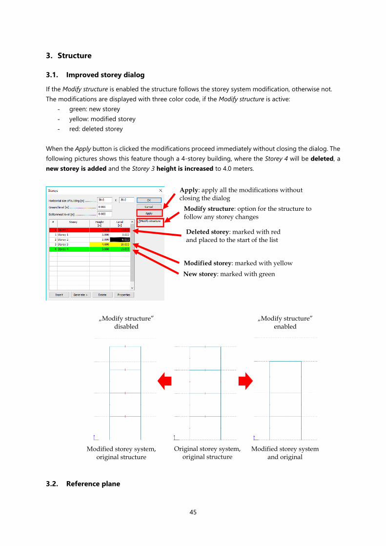
If the Modify structure is enabled the structure follows the storey system modification, otherwise not.
The modifications are displayed with three color code, if the Modify structure is active:
- green: new storey
- yellow: modified storey
- red: deleted storey
When the Apply button is clicked the modifications proceed immediately without closing the dialog. The
following pictures shows this feature though a 4-storey building, where the Storey 4 will be deleted, a
new storey is added and the Storey 3 height is increased to 4.0 meters.
3.2. Reference plane
Modify structure: option for the structure to follow any storey changes
Apply: apply all the modifications without closing the dialog
Deleted storey: marked with red and placed to the start of the list
Modified storey: marked with yellow
New storey: marked with green
Original storey system, original structure
„Modify structure” enabled
„Modify structure” disabled
Modified storey system and original
Modified storey system, original structure

46
Reference plane is an auxiliary object, which allows User to align elements to it. It can be found in the
Structure tab.
As is it shown below, Description of Reference plane can be typed in the tool palette or after clicking on
the Default properties button, it can be set in the new dialog.
Reference plane can be drawn in any plane. It is displayed by the region contours and its description
given by the user.
The Reference plane can be used with the feature Align region to plane. (Modify/Modify region/Align
region to plane/Pick region to align/Select Reference plane - See chapter 2.6) and it also can be used
by Correct model tool to fit structural objects to.
Reference planes can be exported into/imported from Autodesk Revit via struxml
format.
47
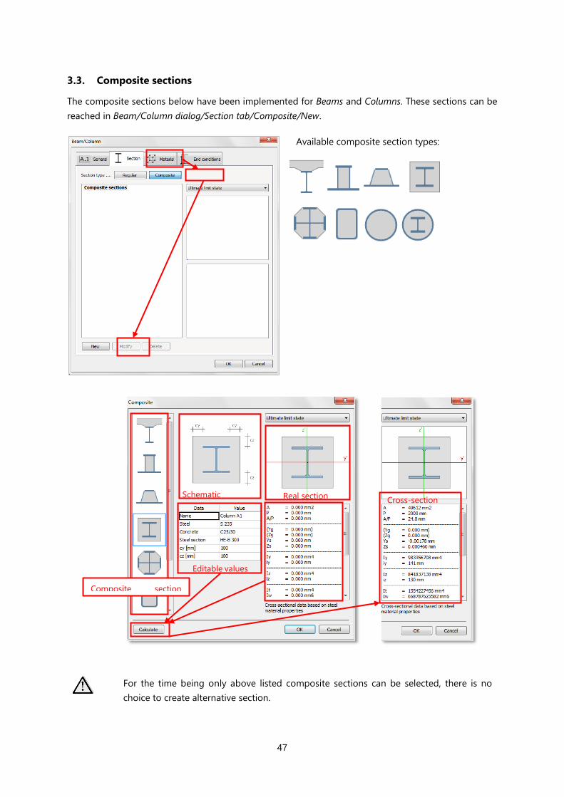
3.3. Composite sections
The composite sections below have been implemented for Beams and Columns. These sections can be
reached in Beam/Column dialog/Section tab/Composite/New.
Available composite section types:
For the time being only above listed composite sections can be selected, there is no
choice to create alternative section.
Schematic Real section
Composite section
Editable values
Cross-section

48
3.4. Pile
In FEM-Design 17, a new structural element is added - the pile. Its main purpose is to calculate pile
internal forces in either linear or non-linear way (e.g. limited shaft friction, only compression behaviour
at the tip of pile can be considered).
The basic concept is that the soil surrounding the pile is modelled with continuous line supports along
it. These supports stand for the supporting effect of the soil together with a vertical point support at the
tip of pile. The new plastic element feature offers a more precise way to calculate the internal forces by
considering the nonlinear characteristic of the soil-structure interaction.
This feature can be found among the Foundation objects on Structure tab.
Piles can be placed either one by one, or in groups using the “Array rectangular”/ “Array polar” options.
In the Tool window User can declare the Height of the pile and set the array options as Column distance,
Row distance and Angle of array.
If choosing Array rectangular define option, at first User needs to set the Column and Row distances,
before placing the piles. By clicking these textboxes turn active.

49
If choosing Array polar, two more options become available according to the following figure:
To open Pile dialog click Default settings.
On General tab User can give an identifier and a rotation angle.
Regular and certain types of composite sections can be selected in Section tab/Composite/ New.

50
The available composite sections for simple pile are the followings:
The material can be selected in the same way as for Beams/Columns.

51
On the End conditions tab User can set the top release of the pile, which can be useful in case piles are
connected to a foundation slab. The connection can be either fixed or hinged.
The program generates a set of line support groups
for the pile (at least one for each stratum with an
additional breakpoint at the highest water level) and
one point support at the tip of the pile. If the pile is
edited or some changes happen in the input data
(e.g. changing of the material of a stratum), these
stiffness and plastic limit values will be recalculated.
The automatic calculation can be switched off in Pile
dialog/Soil springs tab/Auto calculate checkbox.
The Soil springs tab will be active only after placing the pile and its properties is displayed
in the dialog.
From the previously defined strata, FEM-Design calculates the stiffness and plastic limit values for both
the line and point supports.

52
The line support groups along the pile have only translational stiffness, Kx’ vertical (shear) and Ky’, Kz’
horizontal stiffness [kN/m/m]. For the horizontal spring stiffness, it does not have any practical sense to
define compression and tension stiffness, thus for the horizontal directions (y’, z’) one value defines each
direction. The horizontal stiffness of the line support in y’ direction (similar in z’ direction):
𝐾𝑦′ = 𝑘𝑠,𝑦′ ∙ 𝐵 [
𝑘𝑁
𝑚2]
where B is the width of the pile and ks,y’ is the horizontal coefficient of subgrade reaction. According to
Vesic (1961), it can be calculated by using both soil and pile properties:
𝑘𝑠,𝑦′ =0.65 ∙ 𝐸𝑠
𝐵 ∙ (1 − 𝜇𝑠2)
∙ [𝐸𝑠 ∙ 𝐵4
𝐸𝑝 ∙ 𝐼𝑝,𝑧′]
112
[𝑘𝑁
𝑚3]
where Es and µs is the Young’s modulus and Poisson’s ratio of the soil, Ep and Ip,z’ are the Young’s modulus
and moment of inertia of the pile.
The vertical behaviour, thus the vertical spring stiffness might be different for compression and tension,
so both spring stiffness are available for the User to define (for example One may want to neglect the
friction forces for tensioned piles). Based on the analytical solution of Zhang Q. et al. (2014), the vertical
stiffness of the line support is:
𝐾𝑥′ = 𝑘𝑠 ∙ 𝑃 = 𝐺𝑠
𝑟0 ∙ 𝑙𝑛 (𝑟𝑚
𝑟0)
∙ 𝑃 [𝑘𝑁
𝑚2]
where Gs is the shear modulus of the soil, r0 is the pile radius (or equivalent radius for noncircular piles),
rm is the radial distance at which shear stresses in the soil become negligible and P is the perimeter of
the cross section of the pile. In the different soil layers, rm distance can be calculated as the following:
𝑟𝑚 = 2.5 ∙ 𝐿 ∙ 𝜌𝑚 ∙ (1 − 𝜇𝑠)
where L is the (total) length of the pile, ρm is the factor of vertical homogeneity of soil stiffness and µs is
the Poisson’s ratio of soil layer around the pile. The value of ρm can be calculated in the following way:
𝜌𝑚 =𝐺𝑠,𝑚𝑖𝑑𝑑𝑙𝑒
𝐺𝑠,𝑏𝑜𝑡𝑡𝑜𝑚
where Gs,middle is the shear modulus at the middle of the layer and Gs,bottom is the shear modulus at the
bottom of the layer (relevant only in case of soils with variable material properties with height).
The point support at the tip of the pile has only vertical (or in case of skew piles only x’ directional)
stiffness. The tension stiffness is set to zero by default as tension forces are not transmitted between the
soil and the tip of the pile. Zhang Q. et al. (2014) suggest the following formulae to use for the
compression stiffness:
𝐾𝑥′ =4 ∙ 𝐺𝑠 ∙ 𝑟0
(1 − 𝜇𝑠) [
𝑘𝑁
𝑚]
Besides the spring stiffness, plastic limit values are also calculated for both line and point supports. For
the vertical line support the plastic limit value is based on the shaft friction, for the point support at the
tip of the pile it depends on the end bearing of the pile. In both cases the calculation is affected by the
behaviour of the soil (drained/undrained), as it is summarized by Wrana B (2015).

53
In case of undrained soil the limit value is based on the undrained shear strength (cuk). The limit value of
the line support:
𝑃𝑙𝑖𝑚,𝑥′ = 𝑞𝑠 ∙ 𝑃 = 𝛼 ∙ 𝑐𝑢𝑘 ∙ 𝑃 [𝑘𝑁
𝑚]
where qs is the shaft friction and α is the adhesion coefficient. The latter one is calculated according to
the proposition of the NAVFAC DM 7.2 (1984), the corresponding details can be found in the literature.
The limit value of the point support (for compression):
𝑃𝑙𝑖𝑚,𝑥′ = 𝐴𝑏𝑎𝑠𝑒 ∙ 𝑐𝑢𝑘 ∙ 𝑁𝑐 [𝑘𝑁]
where Abase is the cross-sectional area of the pile (at the tip), Nc is the bearing capacity coefficient that
can be assumed equal 9.0 according to Skempton (1959).
In case of drained soil the resistances are based on the internal friction angle (φk) and cohesion (ck) of
the soil layers. The limit value of the line support:
𝑃𝑙𝑖𝑚,𝑥′ = 𝑞𝑠 ∙ 𝑃 = 𝛽 ∙ 𝜎𝑣′ ∙ 𝑃 [
𝑘𝑁
𝑚]
where σv’ is the vertical effective stress and β is a friction coefficient multiplier. As the vertical stresses
are increases with the depth, an average value of the current layer is used in the equation. At water level
vertical stresses have a break point, thus at the generation of line supports this point is always considered
in such a way that it is the start/endpoint of the neighbouring line supports.
Only the highest water level is considered in the calculation of plastic limit values and
negative shaft friction forces.
The value of β is taken according to the NAVFAC DM 7.2 (1984). The limit value of the point support (for
compression):
𝑃𝑙𝑖𝑚,𝑥′ = 𝐴𝑏𝑎𝑠𝑒 ∙ 𝑞𝑏 = 𝐴𝑏𝑎𝑠𝑒 ∙ (𝜎𝑣′ ∙ 𝑁𝑞 + 𝑐𝑘 ∙ 𝑁𝑐) [𝑘𝑁]
Where
𝑁𝑐 = (𝑁𝑞 − 1) ∙ cot 𝜙𝑘
where Nq is the bearing capacity factor, and according to the NAVFAC DM 7.2 (1984), its value depends
on the fabrication technology of the pile and the internal friction angle of the soil.
54
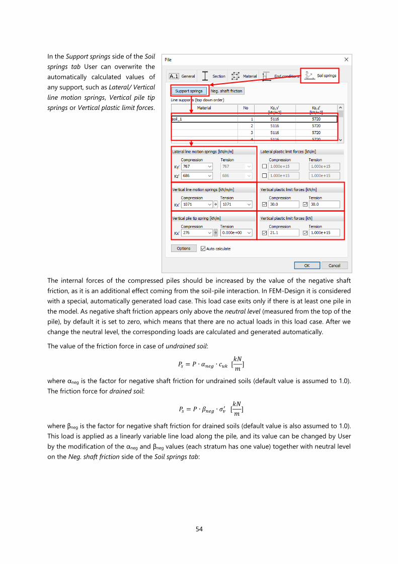
In the Support springs side of the Soil
springs tab User can overwrite the
automatically calculated values of
any support, such as Lateral/ Vertical
line motion springs, Vertical pile tip
springs or Vertical plastic limit forces.
The internal forces of the compressed piles should be increased by the value of the negative shaft
friction, as it is an additional effect coming from the soil-pile interaction. In FEM-Design it is considered
with a special, automatically generated load case. This load case exits only if there is at least one pile in
the model. As negative shaft friction appears only above the neutral level (measured from the top of the
pile), by default it is set to zero, which means that there are no actual loads in this load case. After we
change the neutral level, the corresponding loads are calculated and generated automatically.
The value of the friction force in case of undrained soil:
𝑃𝑠 = 𝑃 ∙ 𝛼𝑛𝑒𝑔 ∙ 𝑐𝑢𝑘 [𝑘𝑁
𝑚]
where αneg is the factor for negative shaft friction for undrained soils (default value is assumed to 1.0).
The friction force for drained soil:
𝑃𝑠 = 𝑃 ∙ 𝛽𝑛𝑒𝑔 ∙ 𝜎𝑣′ [
𝑘𝑁
𝑚]
where βneg is the factor for negative shaft friction for drained soils (default value is also assumed to 1.0).
This load is applied as a linearly variable line load along the pile, and its value can be changed by User
by the modification of the αneg and βneg values (each stratum has one value) together with neutral level
on the Neg. shaft friction side of the Soil springs tab:

55
If User clicks on Option, the Pile option dialog opens. Here User can select the Type of pile, declare the
Surface surcharge (affecting the vertical stresses in case of drained soils), the division length of line
supports and can decide the method of the Section perimeter’s calculation. Division length becomes a
very important setting in case on plastic analyses. The plastic limit forces are increasing with depth, but
along a line support it is constant. Consequently, the more line supports are created along the pile (with
the automatically calculated, increasing limit values) the more accurate plastic distribution of internal
forces we get.
56
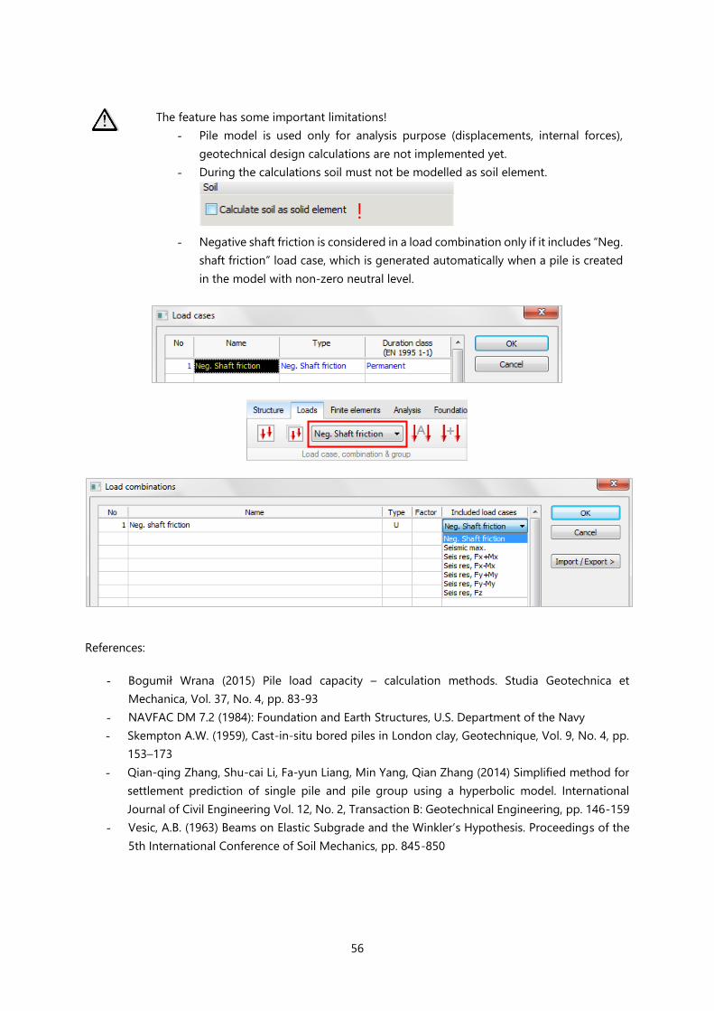
The feature has some important limitations!
- Pile model is used only for analysis purpose (displacements, internal forces),
geotechnical design calculations are not implemented yet.
- During the calculations soil must not be modelled as soil element.
- Negative shaft friction is considered in a load combination only if it includes “Neg.
shaft friction” load case, which is generated automatically when a pile is created
in the model with non-zero neutral level.
References:
- Bogumił Wrana (2015) Pile load capacity – calculation methods. Studia Geotechnica et
Mechanica, Vol. 37, No. 4, pp. 83-93
- NAVFAC DM 7.2 (1984): Foundation and Earth Structures, U.S. Department of the Navy
- Skempton A.W. (1959), Cast-in-situ bored piles in London clay, Geotechnique, Vol. 9, No. 4, pp.
153–173
- Qian-qing Zhang, Shu-cai Li, Fa-yun Liang, Min Yang, Qian Zhang (2014) Simplified method for
settlement prediction of single pile and pile group using a hyperbolic model. International
Journal of Civil Engineering Vol. 12, No. 2, Transaction B: Geotechnical Engineering, pp. 146-159
- Vesic, A.B. (1963) Beams on Elastic Subgrade and the Winkler’s Hypothesis. Proceedings of the
5th International Conference of Soil Mechanics, pp. 845-850
!

57
3.5. Horizontal bedding moduli of foundation slab
In the properties dialog of the Foundation slab a new option has been added.
From now, besides the vertical bedding modulus, the horizontal one can be specified by the User, instead
of making them equal to the vertical one. These three values define the motion spring stiffness of the
automatically created surface support group under the foundation slab. By default, the horizontal values
are the half of the vertical one.
This modification has a strong connection with the recently added Pile element. If User would like to
model a pile group connected to a foundation slab, the reduction of the horizontal stiffness of the
foundation slab can be reasonable. As piles have horizontal supporting directly by the surrounding
soil, they are able to carry either the total or a portion of the total horizontal loading.
58
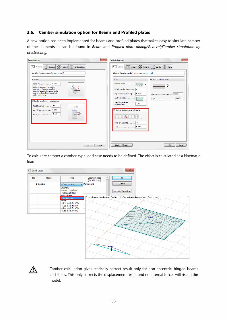
3.6. Camber simulation option for Beams and Profiled plates
A new option has been implemented for beams and profiled plates thatmakes easy to simulate camber
of the elements. It can be found in Beam and Profiled plate dialog/General/Camber simulation by
prestressing.
To calculate camber a camber-type load case needs to be defined. The effect is calculated as a kinematic
load.
Camber calculation gives statically correct result only for non-eccentric, hinged beams
and shells. This only corrects the displacement result and no internal forces will rise in the
model.

59
3.7. Easier definition of column corbel’s load position
The column corbel’s load position is measured from the column axis, instead of the edge of the corbel,
which is easier to define.
In version 16:
In version 17:

60
3.8. Post-tensioned cable
3.8.1. General
Modelling
Post-tensioned cable object (hereinafter PTC) is a structural component, modelled by equivalent load
system.
Currently the unbonded structural design modelling is available.
The object contains of the shape (continuous line), the reference line (dashed line) and an arrow marking
the active end.
The following figure shows a post-tensioned beam after jacking: the actions on the cable a), the actions
on the structure b) and the modelled forces acting on the reference line c).
Besides the equivalent forces in
the local z direction from the
angular deviation, the
neglected x’ component of the
angular deviation, the friction
force, and moment caused by
the friction force - cable
eccentricity (relative to the
reference line) could be
significant along the reference
line.
The plane of the shape can be modified by using “Change direction” or “Rotation”
functions.
The definition of a PTC automatically creates two load cases:
- PTC T0: Initial stress state (after the jacking process, it contains the short term stress losses)
- PTC T8: At the end of the design lifetime (it contains the time-depenedent stress losses)
61
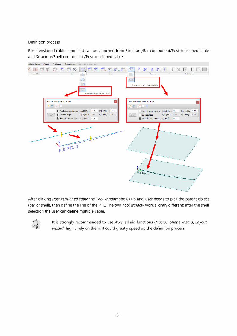
Definition process
Post-tensioned cable command can be launched from Structure/Bar component/Post-tensioned cable
and Structure/Shell component /Post-tensioned cable.
After clicking Post-tensioned cable the Tool window shows up and User needs to pick the parent object
(bar or shell), then define the line of the PTC. The two Tool window work slightly different: after the shell
selection the user can define multiple cable.
It is strongly recommended to use Axes: all aid functions (Macros, Shape wizard, Layout
wizard) highly rely on them. It could greatly speed up the definition process.
62
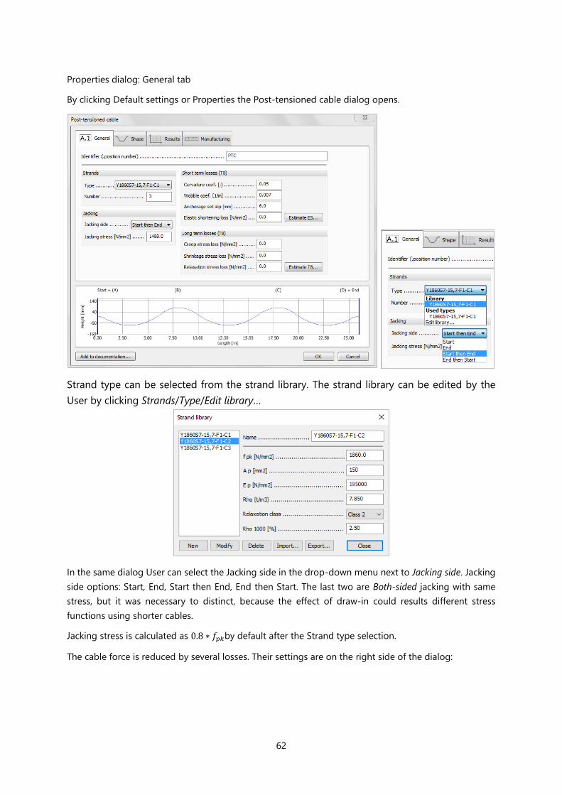
Properties dialog: General tab
By clicking Default settings or Properties the Post-tensioned cable dialog opens.
Strand type can be selected from the strand library. The strand library can be edited by the
User by clicking Strands/Type/Edit library…
In the same dialog User can select the Jacking side in the drop-down menu next to Jacking side. Jacking
side options: Start, End, Start then End, End then Start. The last two are Both-sided jacking with same
stress, but it was necessary to distinct, because the effect of draw-in could results different stress
functions using shorter cables.
Jacking stress is calculated as 0.8 ∗ 𝑓𝑝𝑘by default after the Strand type selection.
The cable force is reduced by several losses. Their settings are on the right side of the dialog:

63
Short term losses (initial, T0):
- friction: It is estimated by EN 1992-1-1 5.10.5.2 (1) (formula 5.45) using the Wobble (k)
and Curvature coefficients (µ):
∆𝑃𝜇(𝑥) = 𝑃𝑚𝑎𝑥 + (1 − 𝑒−𝜇(𝜃+𝑘𝑥))
- anchorage set slip
- elastic shortening
Long term, time dependent losses (final, T8):
- shrinkage of structure
- creep of structure
- relaxation of post-tensioned cable
The Elastic shortening loss and Long term losses can be estimated by the specific dialog.
Elastic shortening loss can be estimated by Estimate ES… button. This dialog is automatically filled with
the parent object’s data. Calculate stress values are the result of the estimation and the Elastic shortening
stress loss field is applied on the General tab if the User accepts. It uses modified EN 1992-1-1 5.10.5.1.
(2) (formula 5.44) to handle sparsely placed cables:
∆𝜎𝑒𝑙 = 𝐸𝑝 ∑ [𝑗∆𝜎𝑐
𝐸𝑐𝑚
]
𝑖𝑓 𝑛 ≥ 2 𝑡ℎ𝑎𝑛 𝑗 =𝑛 − 1
2𝑛𝑒𝑙𝑠𝑒 𝑗 = 0.5𝑛
Where n is the Number of strand.

64
Average stress in the structure (𝜎𝑐) is informative only.
Long term losses can be estimated by the Estimate T8… This dialog works as the previous one: fields are
filled with the parent object’s data and the calculated results are at the bottom (Relaxation information
is in the Strand library). It uses EN 1992-1-1 5.10.6 (2) (formula 5.46). The summation of the calculated
long term losses is equal to the result of this interaction formula.
Estimation dialogs calculate cross section data for 1m wide stripes if plate object is the parent.
Both estimation dialog is available during the Default settings editing, edit fields are filled with zeros.
Properties dialog: Shape tab
On the Shape tab there are settings related to the geometry of the cable.
The Shape table can contain Base points and Inflection places: these determine whether linear or
parabolic shape is applied.
Base point: A point with exact position, user known x’ – z’ coordinates and the angle of the
tangent. Usually minimum and maximum places and end points. (Black rectangles in the
preview.)
Inflection place: A function connection place (xinf), where user defines x coordinate only. Using it between
Base points determines two parabolic function: fn and fn+1 where C1 continuity is fullfilled: fn(xinf) =
fn+1(xinf), f’n(xinf) = f’n+1(xinf). (Blue circles in the preview.)
65
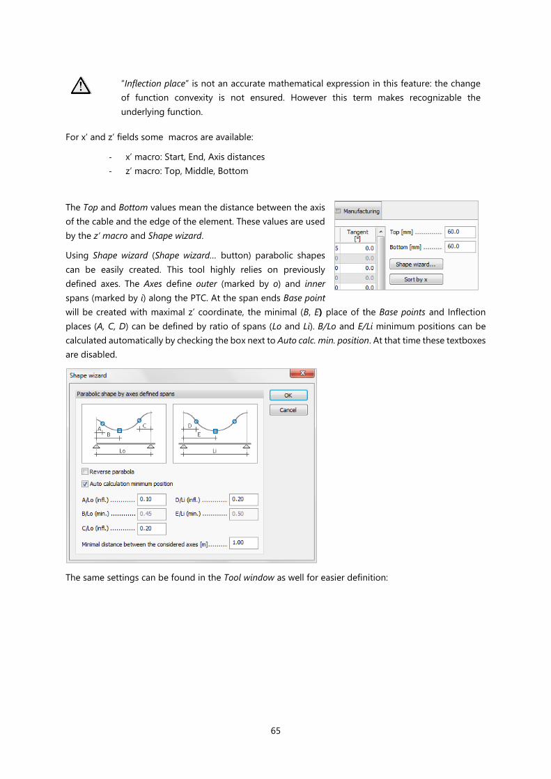
“Inflection place” is not an accurate mathematical expression in this feature: the change
of function convexity is not ensured. However this term makes recognizable the
underlying function.
For x’ and z’ fields some macros are available:
- x’ macro: Start, End, Axis distances
- z’ macro: Top, Middle, Bottom
The Top and Bottom values mean the distance between the axis
of the cable and the edge of the element. These values are used
by the z’ macro and Shape wizard.
Using Shape wizard (Shape wizard… button) parabolic shapes
can be easily created. This tool highly relies on previously
defined axes. The Axes define outer (marked by o) and inner
spans (marked by i) along the PTC. At the span ends Base point
will be created with maximal z’ coordinate, the minimal (B, E) place of the Base points and Inflection
places (A, C, D) can be defined by ratio of spans (Lo and Li). B/Lo and E/Li minimum positions can be
calculated automatically by checking the box next to Auto calc. min. position. At that time these textboxes
are disabled.
The same settings can be found in the Tool window as well for easier definition:

66
It is not recommended to use Beam/Apply default physical alignment option for beam
containing PTC, since it can cause unnecessary eccentricity in the shape because Shape
wizard uses the physical element.
By allowing the Display physical element optionthe section of the cross-sectioned element is shown.
Display physical element option shows all cross-sectioned element, the parent object is
signed by dark-grey, the non-parents are signed by light-grey.
The Equilibrium status and Minimal radius of curvature are also displayed.
67
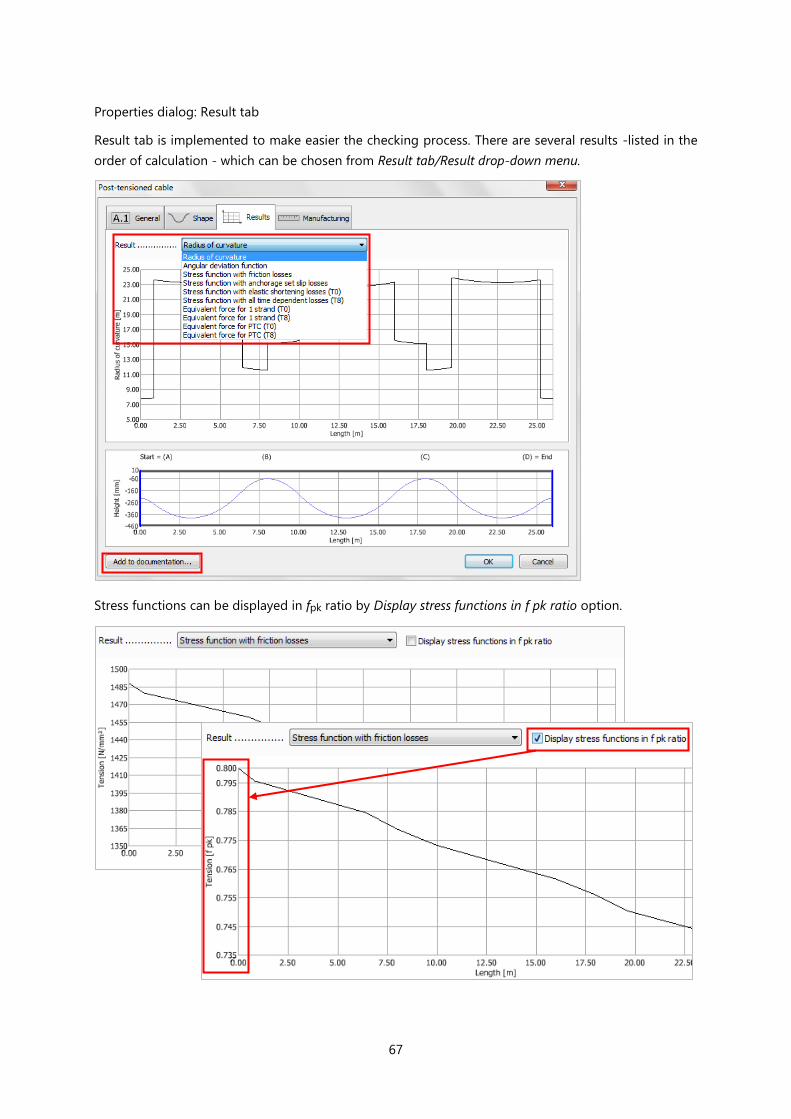
Properties dialog: Result tab
Result tab is implemented to make easier the checking process. There are several results -listed in the
order of calculation - which can be chosen from Result tab/Result drop-down menu.
Stress functions can be displayed in fpk ratio by Display stress functions in f pk ratio option.

68
The example shows a typical Stress function in the T8 state and an Equivalent force at T0
state.

69
Properties dialog: Manufacturing tab
On this tab the Manufacture drawing can be set with proper x’ and z’ shift.
The Manufacture drawing can be exported into AutoCAD by clicking Export…

70
To fine the division section points can be inserted along the cable. Click Generate points to open the
dialog. At the third option the division-distance can be set by the User.

71
The position of each point can be edited with Edit points button. By clicking Sort button the points will
be sorted by their x’ value in increasing order.
72
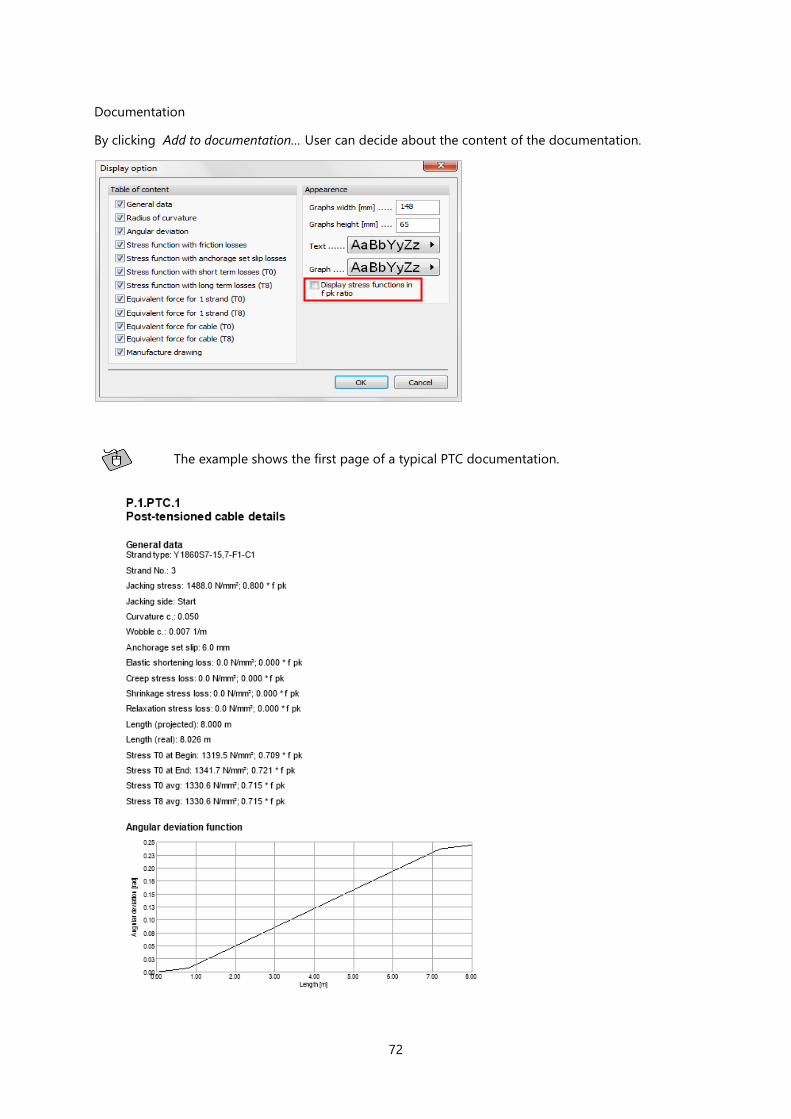
Documentation
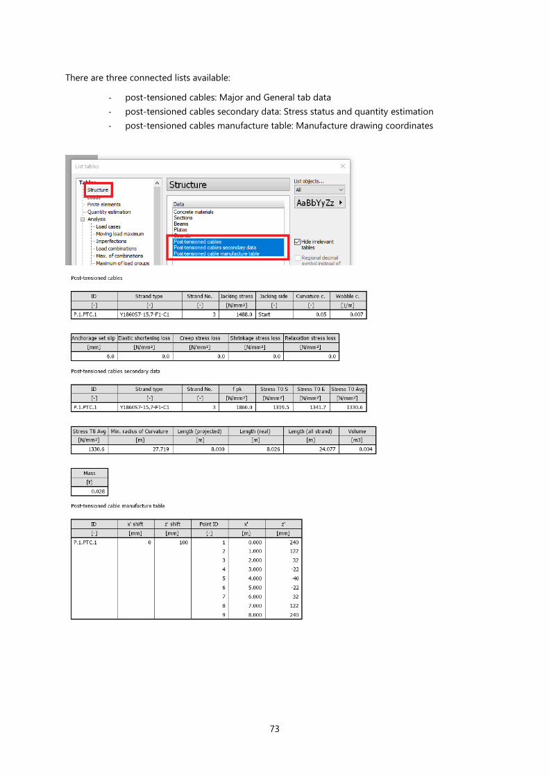
By clicking Add to documentation… User can decide about the content of the documentation.
The example shows the first page of a typical PTC documentation.
73
There are three connected lists available:
- post-tensioned cables: Major and General tab data
- post-tensioned cables secondary data: Stress status and quantity estimation
- post-tensioned cables manufacture table: Manufacture drawing coordinates

74
Handling multiple PTCs properties
If the PTC-s have the same settings, length and shape, all features of properties dialog are available,
otherwise only the common properties appear.
Add to documentation… and Manufacture tab/Export… functions are available at multiple
selection and they document all selected cables at the same time.
Others
Post-tensioned cable option is added to the Colour schema. Available colour modes: ID, Strand type,
Strand number, Jacking side.
PTCs can be selected by several option of the Filter: Structural element, Identifier, Strands
PTCs have detailed tooltips supplemented by length and Stress status (connected chapters from the EN
1992-1-1: 5.10.2.1 (1) and 5.10.3 (2)).

75
3.8.2. Layout wizard
It is a parametric tool to create a set of PTCs in a specific layout at the same time. It can be launched
from Structure/Shell component/Post-tensioned cable/Layout wizard.
The Layout wizard searches the closest solution to the Unequal loading settings from the PTC layout
variations which fulfilled the following conditions:
- difference between the sum of the PTC’s forces acting in local z+ direction and the
product of Considered load and Balance ratio is less than the Maximal deviation
- geometrical requirements
The Layout calculation process shows the currently calculated layout parameters and a few indicator
values. After the calculation it shows the parameters of the best found solution.
Select
plate

76
The function uses Axes to divide the selected structural element to stripes (Mid span and Column span)
assuming columns in the axes cross points.
The algorythm can handle the holes of the plate regions.
At least two Axes crossing the plate are needed to use this function.
Checking Shape wizard using height [mm] instead of physical model option could highly
reduce the runtime if the selected plate’s thickness is constant.
3.9. “No shear” edge macro for Plane walls
“No shear” macro has been added to the Edge list of Plane wall edit tools. Using it defines edge
connection with predefined “No shear” rigidity type on the defined wall’s bottom edge.
It is the recommended wall definition method to create a non-bracing system element.
The following example shows a displacement graph of a multi-storey building where W.4
wall is not part of the bracing system.
77
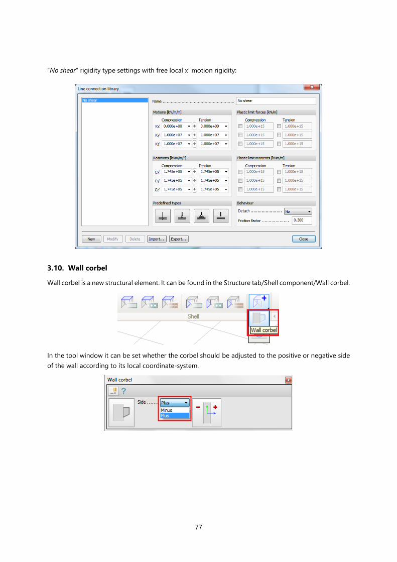
“No shear” rigidity type settings with free local x’ motion rigidity:
3.10. Wall corbel
Wall corbel is a new structural element. It can be found in the Structure tab/Shell component/Wall corbel.
In the tool window it can be set whether the corbel should be adjusted to the positive or negative side
of the wall according to its local coordinate-system.

78
Wall corbel can be placed on Plane wall only.

79
3.11. Editable surface connection (soil)
Stiffness properties of automatically generated surface connections are editable.
The example shows a settled foundation slab into soil.
Right click on the surface connection, then select Properties (see chapter 2.1.).
1.
2
.

80
4. Load
4.1. Construction stages
The Construction stages function helps to model and design the different building phases, and it helps
to determine the construction process affected displacement/internal force distribution of the finished
structure. Currently we implemented this feature for high-rise buildings, making the structural
element separation by the storey system, but it will be generalized to a user-defined stage system
in the near future.
Storeys must be defined to use Construction stages, since currently one storey is considered as one
Stage.
Construction stages can be defined under the load tab. Click “Generate” button to create stages with
the correspondent storey name.
Columns in the table mean the following:
- No: Number of the stage
- Stage description: Name of storey which is built in the stage
- I (Initial stress): if checked, in calculation of the stage displacements will be reset to zero, but
other results (internal forces) are accumulated
- Activated load cases: Activated load cases for the stage
- Partitioning:
This defines for each load from the load cases that how and when it is activated during the
construction stage calculation.
o only in this stage: Load case is activated in the specified construction stage and acts only
in this stage.
Adding loads to stages
Loads in each stage

81
o from this stage on: Load case is activated in the specified construction stage and acts in
this and also in the remaining stages – the parts of the loads that act on the previous
storeys are also activated in the specified stage
o shifted from first stage: Load case is activated in the specified construction stage and
acts in this and also in the remaining stages – the parts of the loads that act on the first
storey will act in this specified stage and the remaining parts of the loads that act on
the second storey will act in the next stage and so on (e.g.: flooring and covers)
Remaining loads from these load cases will not activate in other
stages.
q1
q2
q3
q4
q1
q2
Only in this stage (applied in 2nd stage)
CS.1 CS.2 CS.3 CS.4
q1
q2
q3
q4
CS.1 CS.2 CS.3 CS.4
From this stage on (applied in 2nd stage)
q1
q2
q3
q4

82
It is possible to add any construction stage to any load combination with the following limitations:
- Only one construction stage is allowed in one combination.
- Cannot combine a construction stage and a load case which is already activated in a construction
stage
- The fire and/or seismic load cases can be combined with only the final construction stage
For load groups only the final construction stage can be added too.
The construction stages automatically follow all storey modifications.
User can start the construction stage calculation at Analysis/Calculation/Construction stages. There are
two calculation methods, so called Incremental “Tracking” method and “Ghost” structure method.
When incremental method is chosen, the model is built stage-by-stage. In case of “ghost” structure
method the full structure is in the calculation, but stiffness of those structural parts which aren’t in the
specific stage is highly reduced.
Incremental “Tracking” method
q1
q2
q3
CS.1 CS.2 CS.3 CS.4
Shifted from first stage (applied in 2nd stage)
q4
q3
q4
q2
q1

83
“Ghost” structure method
The construction stage results can be found in the New results/Analysis/Construction stages. For every
stage result the method name and the displayed construction stage (e.g. CS.1 Storey 1) appears in the
information panel.
Adding any new Construction stage result will open a "Construction stages" (result-display) tool to make
easier the navigation between the stage results and to animate the Construction process if it is needed.
It’s also possible to choose the construction stage in detailed results.

84
The equilibrium dialog contains the construction stages, too.
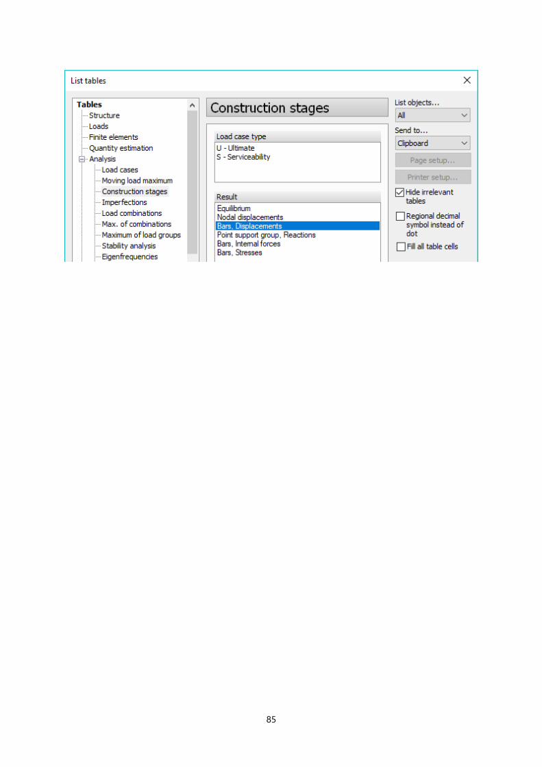
It’s possible to list the construction stages result, which can be found under Analysis/Construction stages.
85

86
4.2. Pre defined Psi values for temporary load groups
There is an option for temporary load groups to choose predefined ψ0, ψ1 and ψ2 values.
4.3. Ignored temporary load cases
Temporary load groups has an option to ignore in SLS combinations in Load group maximum results
and in Generating load combinations by load groups.
4.4. Deviation load improved
There are changes in deviation load macro.
- User can set the value of “m” instead of “alpha m”, which is calculated automatically from “m”.
The applied values can be given for each storey, which will be stored.
- A checkbox has been implemented, which allows generation of surface load instead of point
load.

87
- Loads can be defined in positive and/or negative direction, which can be applied with the
plus/minus buttons next to the icons , in the bottom-right corner of the dialog.
As many load cases will be generated as many buttons are checked.
1.
2.
3.

88
4.5. Notional load
This function generates horizontal load from non-horizontal loads using a conversion factor.
It can be reached in Load tab/Macro/Notional load.
- For the notional load case a name can be given by typing it into the textbox on top of the dialog
- After clicking EC seismic notional load button, Load case factor will be set according to
parameters of Load groups the Load case belongs to. It uses EN 1990-1-1 A1.3.2 DK NA: 𝐴𝑑 =
1.5%(∑ 𝐺𝑘,𝑗" + " ∑ 𝜓2,𝑖𝑄𝑗,𝑖𝑖≥1 )
- After clicking on the Generate button, as many Notional Load cases will be created, as many
directions are chosen above the Generate button
The generated Notional Load Cases appear in the Load Cases dialog and they can be selected from Loads
tab/Current load case drop-down list.
The process of the load generation by Notional load macro is shown on the picture below.
1.
2.
3.

89

90
4.6. Load comments
A new property – Comment - has been added to all load types. With this new feature the User can label
every single load in order to easily identify them.
The comments can be set for every load types in the Default settings/Properties dialog.
Load comments can be turned on/off by Settings/Display/Load dialog’s Display comment option.
Load comments appear in the Filter dialog and also in the listed load tables.

91
4.7. Load export / import via clipboard
Load Export and Import via clipboard is implemented, to let the user easily and quickly modify loads.
In order to export loads, User has to click to Export to send the load information to the clipboard. Then
User can paste to Excel or any editor program and modify them.
Only comments and the load intensities can be modified. We suggest NOT to edit other
columns to avoid errors in Importing.
After changing attributes, User can choose whether to import some. or all of the loads by selecting the
desired rows and copying them to clipboard, then in FEM-Design clicking on Import.
If the User exported constant surface load, only changing the first intensity value will have
effect on the surface load.
Export Import
Editable columns

92
5. Analysis
5.1. Plastic trusses, supports and connections
Plastic calculation has been implemented for trusses, supports and connections.
It is also available for edge connections of all shell elements (Plane plate and wall, Profiled plate and
wall, Timber plate and wall, Fictitious shell)
The plastic data can be set in the Default settings/Data tab of each above mentioned options. The figures
show where the feature is placed in the three types of dialogs of these items.
Some examples with detailed calculations can be found in the verification book.
The options above are considered only for load combinations calculated as non-linear elastic. Plastic
behaviour is considered for load combinations calculated as non-linear elastic + plastic. See more details
in the next chapter.
For further information check the documentation.

93
5.2. Modified behaviour of trusses in non-linear elastic (NLE) and non-linear elastic +
plastic (PL) calculations
Limited tension capacity is available for trusses from now on. In the former versions only limited
compression capacity was implemented.
In the earlier versions of FEM-Design in case of NLE (so-called uplift) calculation, if maximal compression
capacity of a truss was set to zero, and in the first iteration step compression arose in the truss due to
the external loads, the calculation method did not allow tension to arise during the further iteration
steps, even if it was theoretically possible. Now it has been implemented that compression and
tension are changing during the iteration in case of NLE calculation.

94
However the actual effect of the two behaviour options (brittle or plastic) depends on the setup of the
specific load combination.
Load
combination
calculation
setup
NLE
NLE + PL
Properties
dialog settings
Behaviour Brittle, independently on which
behaviour is selected in the properties
dialog
Brittle or plastic, depending on which
behaviour is selected in the properties
dialog

95
5.3. Check for identical copies of structural objects and loads
A new option is added to the Settings/All…/Calculation/Analysis dialog. User can set if the program
should check the identical copies of structural elements and/or loads.
For example, let’s take the following example for object multiplication in a model:
- point support: 2 identical supports (1 unnecessary copy)
- line support: 3 identical supports (2 unnecessary copies) 3 objects, 5 unnecessary copies
- beam: 3 identical beams (2 unnecessary copies)
Having this option ON, during pre-processing of calculation, the following question pops up:
The program informs about the number of unnecessary copies. User has three options to select:
- clicking “Yes”, FEM-Design will delete all unnecessary copies automatically,
- clicking “No” will ignore this check, and the calculation will runs without any modification,
- clicking “Cancel” will abort the calculation and allows User to fix the unnecessary objects with the
new feature called Correct model – Delete identical copies, described in Chapter 1.1.

96
5.4. Fully rigid diaphragm
There is a new type of diaphragm calculation: Fully rigid.
Fully rigid diaphragm will ensure the rigid movement of the all objects lying in diaphragm’s region and
move them all together in one plane in any direction (as rigid body). For further information check the
documentation.

97
5.5. Selecting all relevant shapes in Modal analysis
This new feature helps to select all the relevant shapes in the Modal analysis. By clicking the “Select all”
button the program selects all the shapes with non zero modal mass percentage.
This feature is not selecting the dominant shapes, it has to be selected manually.
98
6. RC design
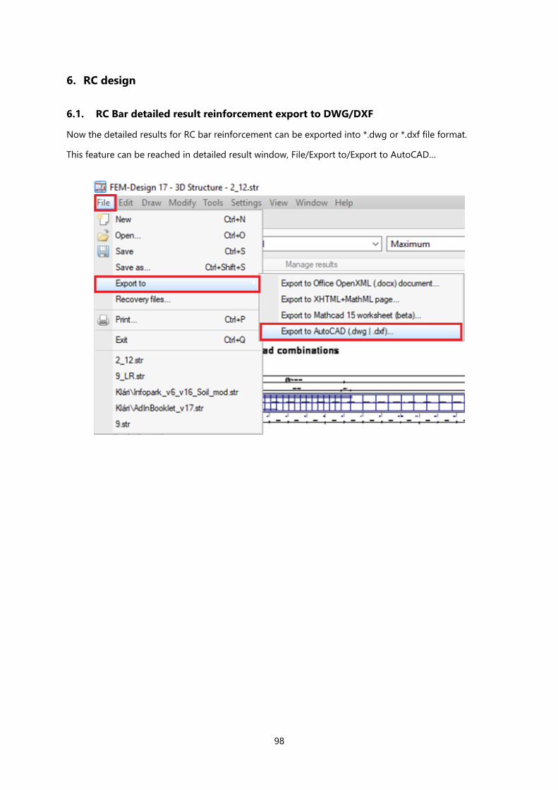
6.1. RC Bar detailed result reinforcement export to DWG/DXF
Now the detailed results for RC bar reinforcement can be exported into *.dwg or *.dxf file format.
This feature can be reached in detailed result window, File/Export to/Export to AutoCAD…
99
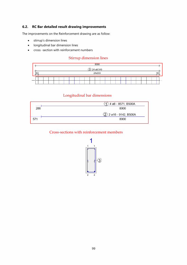
6.2. RC Bar detailed result drawing improvements
The improvements on the Reinforcement drawing are as follow:
• stirrup’s dimension lines
• longitudinal bar dimension lines
• cross -section with reinforcement numbers
Stirrup dimension lines
Longitudinal bar dimensions
Cross-sections with reinforcement members

100
6.3. RC Shell buckling
For the consideration of buckling failure of walls and plates, a new checking criterion is available for RC
shells, the shell buckling. The buckling problem of the shell is transformed to the buckling of equivalent
columns made from the shell, on which the second order resistance and utilization is calculated.
Only RC Plane plates and Plane walls with straight reinforcement and uniform thickness
are suitable for shell buckling calculation.
The calculation process is based on so-called buckling regions, which can be defined at RC
design/Surface reinforcement/Buckling length.
Each buckling region on the shell has a corresponding buckling factor (beta) and a direction vector in
the plane of the shell. The former will be used to calculate the buckling length of the equivalent column,
while the latter one specifies the x’ longitudinal axis of this column. By default, FEM-Design generates
one buckling region on each RC wall and plate. Default buckling direction is vertical on walls, and parallel
with the local x axis on plates. Buckling factor is set to 0.0 on all shells in order to let the User decide
whether this calculation is needed or not, since it is quite time consuming.
Shells with zero buckling factor will not be considered for shell buckling calculation, but
zero utilization is set for them.
The default buckling regions can be modified by adding new regions to the shell. One shell may have
more buckling regions with different beta factor and direction vector, but the shell must be completely
covered by these regions.
During the checking process, the program generates equivalent bar(s) from the shell based on its
material, thickness and reinforcement. This bar is checked as an RC bar: Its utilization is calculated by
determining its second order internal forces and resistance.
The calculation process consists of the following steps:

101
1. As other shell design calculations, the shell buckling is also calculated in every node of the shell
(only where there is a buckling region with non-zero beta value).
2. An equivalent bar is generated for the examined node as follows. The edges of the shell are
intersected by the ray determined by the node and the direction vector of the corresponding
buckling region. The two intersection points are taken as the start and the end point of the
equivalent bars.
Note that this intersection is always made with the edges of the shell and not with the
edges of the buckling region corresponding to the node! If a node is on the border of
two or more buckling regions, it is calculated with both different beta values and direction
vectors, and the higher utilization will be used.
3. The cross section of the equivalent bar is 1 m wide and its height equals to the thickness of the
shell. Along the bar, the applied reinforcement of the shell is transformed into the direction of
the bar and placed into it.
The checking process is executed section by section along the bar. The distance between these
sections is given by Division length of substitute column parameter in Calculation parameter
dialog (see the lower figure). Internal forces acting at these sections are calculated by
β=2
β=2
β=1

102
transforming shell internal forces at the section point into the coordinate system of the column.
As the buckling direction of shells is perpendicular to its plane, we need the equivalent bar’s
normal force and moment vector in the plane of the shell for the calculation.
4. Once the first order internal forces are obtained in every section, the second order internal forces
are calculated based on the nominal stiffness or nominal curvature method, according to the
configuration settings. The only difference in the checking process of a real bar and this
equivalent bar is that now the eccentricity coming from the second order effects are applied
only perpendicularly to the plane of the shell. In other words, the out-of-plane normal force has
eccentricity only along the z’ axis of the shell. This modification is in harmony with the fact that
the buckling direction of the shell is perpendicular to the plane.
5. Finally, based on the second order internal forces, the utilization is calculated for every cross
section of the equivalent bar (based on the interaction curve), and the highest section utilization
is assigned to the node.
Shell buckling calculations are available for Load combinations, Maximum of load combinations and
Maximum of load groups. The utilization results can be displayed in the New result/RC shell/Shell
buckling/Utilization
0.5 m
0.5 m
0.5 m
0.5 m
0.5 m
0.5 m
1.0 m
NEd
MEd,I
NEd
MEd,II

103
Some details of the calculation can be obtained by listing RC design/Load combinations/Shell, buckling
table. Also, wall buckling utilization appears in the Shell, Utilization list.
Every plate and wall has one result, containing the coordinates of the dominant section, the
corresponding reinforcement, first and second order internal forces together with the capacity and
buckling factor.

104
6.4. RC shell – EN 1992-1-1, Annex F
A new checking criterion is added for RC shells according to EN 1992 Annex F.
This feature is meant to inform the user whether the shell reinforcement is optimal or not according to
the EN 1992-1-1, Annex F. The reinforcement is optimal, if the cracks for serviceability limit state are
acceptable and the required deformation capacity for ultimate limit state is provided. This method only
works for in-plane stress state. FEM-Design calculates the stresses in the reinforcement plane. The
program uses the F1.(4) formulas for both the applied and required reinforcement.
Compression is positive in the formulas.
The results can be listed in the RC design for Load Combinations, Max. of combinations and Maximum
of load groups.
If the Danish national annex set in code selection the calculation is based by the 1992-1-
1 DK NA:2007.

105
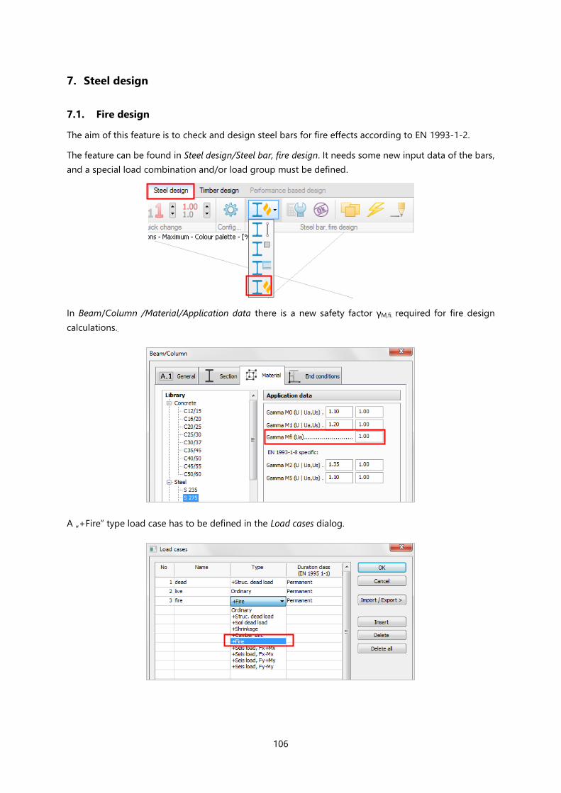
106
7. Steel design
7.1. Fire design
The aim of this feature is to check and design steel bars for fire effects according to EN 1993-1-2.
The feature can be found in Steel design/Steel bar, fire design. It needs some new input data of the bars,
and a special load combination and/or load group must be defined.
In Beam/Column /Material/Application data there is a new safety factor γM,fi. required for fire design
calculations..
A „+Fire” type load case has to be defined in the Load cases dialog.
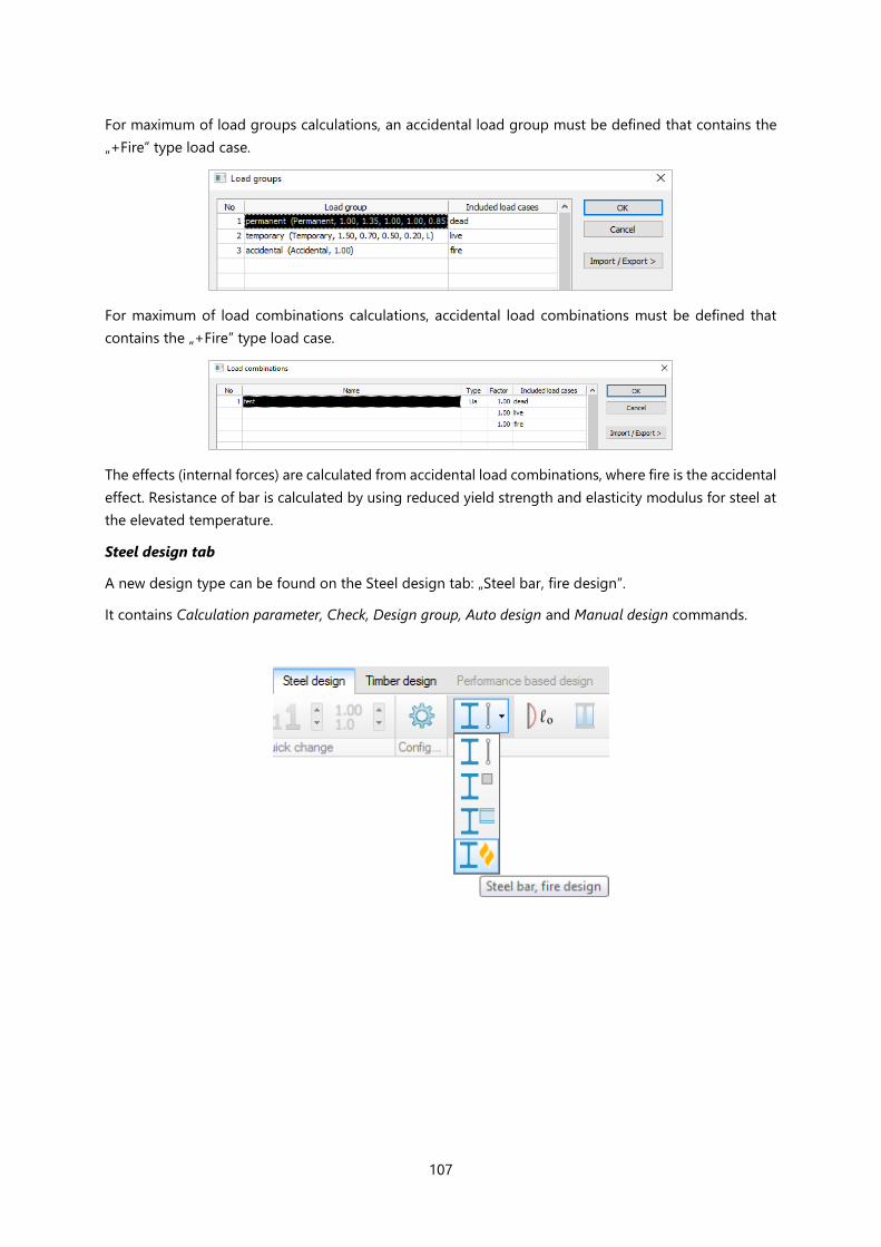
107
For maximum of load groups calculations, an accidental load group must be defined that contains the
„+Fire” type load case.
For maximum of load combinations calculations, accidental load combinations must be defined that
contains the „+Fire” type load case.
The effects (internal forces) are calculated from accidental load combinations, where fire is the accidental
effect. Resistance of bar is calculated by using reduced yield strength and elasticity modulus for steel at
the elevated temperature.
Steel design tab
A new design type can be found on the Steel design tab: „Steel bar, fire design”.
It contains Calculation parameter, Check, Design group, Auto design and Manual design commands.
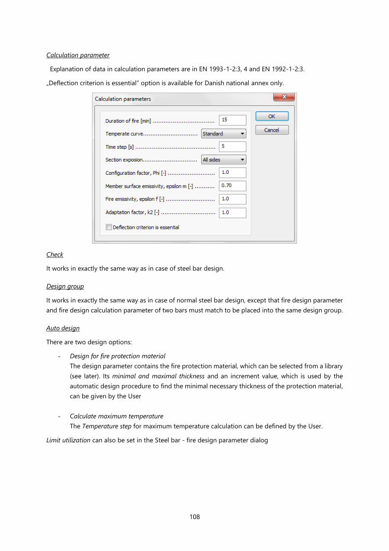
108
Calculation parameter
Explanation of data in calculation parameters are in EN 1993-1-2:3, 4 and EN 1992-1-2:3.
„Deflection criterion is essential” option is available for Danish national annex only.
Check
It works in exactly the same way as in case of steel bar design.
Design group
It works in exactly the same way as in case of normal steel bar design, except that fire design parameter
and fire design calculation parameter of two bars must match to be placed into the same design group.
Auto design
There are two design options:
- Design for fire protection material
The design parameter contains the fire protection material, which can be selected from a library
(see later). Its minimal and maximal thickness and an increment value, which is used by the
automatic design procedure to find the minimal necessary thickness of the protection material,
can be given by the User
- Calculate maximum temperature
The Temperature step for maximum temperature calculation can be defined by the User.
Limit utilization can also be set in the Steel bar - fire design parameter dialog

109
Manual design
Fire protection material (from a library, see later), its thickness, or the Maximum member temperature
can be selected in Steel bar, fire protection dialog for Manual Design..
Fire protection material library
It is available by clicking on „Edit library…” item in the material list of fire protection parameter in Auto
and Manual design dialogs.

110
Results
Utilization results are available to display on the model and to list.
A new result “Max. of combinations/Bar, Combined utilization summary” is available, where the
maximum utilization of steel bars for both normal and fire check is displayed

111
7.2. Steel joint stiffness
FEM-Design 17 gives the opportunity to set the rotation stiffness of Steel Joints automatically or
manually, and apply it to the structure. This feature is available for Steel Joints, where at least one of the
attached bars is connected with its end point by definition.
1. By clicking on the Steel design/Stiffness button, the Steel joint stiffnesses dialog appears.
2. Selecting a joint or joint group in the list will highlight the elements with thick red lines.
3. After that User can double click on the name of a joint/group in the list or just left click on the joint
in the model to open the Set joint stiffness dialog.
Stiffness can be set only for previously calculated Steel Joints!
1.
2.
3.

112
FD 17 uses the calculation method described in the Eurocode 3-8 for calculating joint stiffnesses. This
method is valid only for joints with bolted endplate and column base of I section bars.
The program sets the stiffness of a joint by default as:
- hinged, if it can’t take moment,
- semi-rigid with the calculated value, if it can take moment and stiffness can be calculated
according to EC3-8,
- rigid, if it can take moment but the stiffness cannot be calculated according to EC3-8.
As the calculated stiffness value depends on the load of the joint, FEM-Design 17 by default uses the
load combination that gives the highest utilization for moment. User however, can select another load
combination, or can set stiffness manually.
The details of the calculation can be found in the Detailed result and in the Manual design calculation
dialog.

113
Once the stiffnesses of the joints are set, when leaving design tabs the following dialog will pop up:
Selecting „Yes” will apply the new stiffnesses of joints to the attached bars, if „Apply stiffness to model…”
box is checked in the Set joint stiffness dialog of the joint, or Apply column is checked in the Steel joint
stiffnesses dialog next to the joint/group.
Before joint stiffness calculations
After joint stiffness applied on bar

114
7.3. Column base joint concrete tension failures
New verification is implemented for Column base joints that:
- calculates anchor forces and maximum concrete stress with nonlinear steel and concrete
material behaviour,
- calculates capacities for adhesive and headed anchors for tension failure modes,
- works for both I and RHS sections.
The new parameters required for the new calculations can be found in Design tab.

115
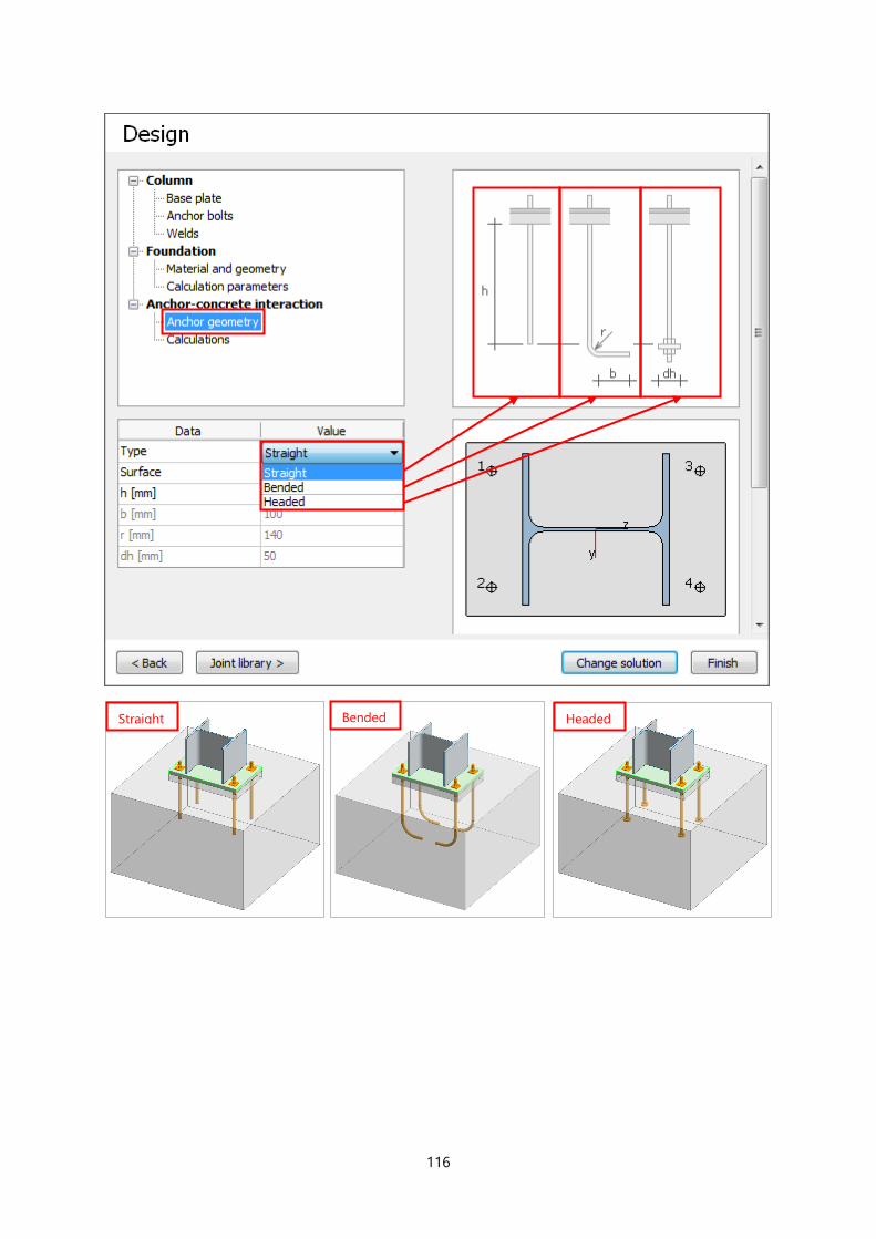
116
Straight Bended Headed
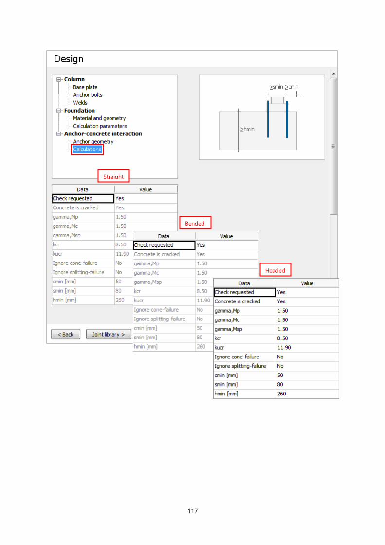
117
Straight
Bended
Headed

118
The picture below shows the output for adhesive (straight or bended) and headed anchorage.
The verification is carried out according to:
- The Swedish Institute of Steel Construction, Detail Handbook, Publication 183, 2.4.1 for the
Straight and Bended type of anchors.
- CEN/TS 1992-4-2: [6.2] for the Headed type of anchors.

119
7.4. “Rotated” option for hollow sections
Hollow sections can be rotated separately in all joints where they are available.

120
7.5. Joint library
Both in Steel joint module and in Steel joint manual design window of 3D Structure module the
customized joint types can be saved into/loaded from a library.
By clicking Save joint, the Save joint to library… dialog opens. In the dialog, in the bottom-left corner an
arbitrary name can be typed for the joint. After clicking Save in the top-right corner, the saved joint
appears in the library.
Library
1
2
.
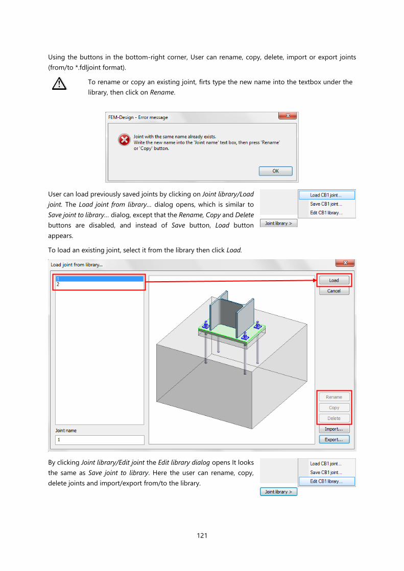
121
Using the buttons in the bottom-right corner, User can rename, copy, delete, import or export joints
(from/to *.fdljoint format).
To rename or copy an existing joint, firts type the new name into the textbox under the
library, then click on Rename.
User can load previously saved joints by clicking on Joint library/Load
joint. The Load joint from library… dialog opens, which is similar to
Save joint to library… dialog, except that the Rename, Copy and Delete
buttons are disabled, and instead of Save button, Load button
appears.
To load an existing joint, select it from the library then click Load.
By clicking Joint library/Edit joint the Edit library dialog opens It looks
the same as Save joint to library. Here the user can rename, copy,
delete joints and import/export from/to the library.

122
In 3D Structure module at Steel design tab/Steel joint/Define joint User can select a joint from the joint
library by checking the Select joint from library checkbox.
In the Load joint from library dialog, only those joints can be chosen thatare compatible with the selected
bar(s). Those joints are shown active (black) in the library.
If User selects a non-appropriate joint for the selected element(s), FEM-Design sends a
warning and automatically creates a joint fitting for the selected item.
Each joint solution has to be saved to its own library. There is no possibility to save all joint
types and solutions into one library.

123
7.6. Steel joints added to Filter
In 3D Structure module steel joints can be filtered either as Joint component, or by their identifier.
7.7. User interface improvements in Steel joints module
7.7.1. Tooltip for joint bars
Tooltip for joint bars has been implemented for easier identification in Steel joint module and Manual
design window in 3D Structure module.

124
7.7.2. Joint bar display option
The positive directions of loads can be displayed on the joint by checking the Display positive direction
of loads option in the Settings/Bars…/Display/Bars dialog in the Steel joint module and in the Manual
design window in the 3D Structure module. The size of the arrows can be set, too.
7.7.3. Navigation buttons for steel joints
In FEM-Design 17, while using Steel joint Manual Design in 3D Structure module, User can switch
between Previous or Next joint by clicking up and down arrows next to the drop-down list.
This feature can be found in Steel Joint module, too.
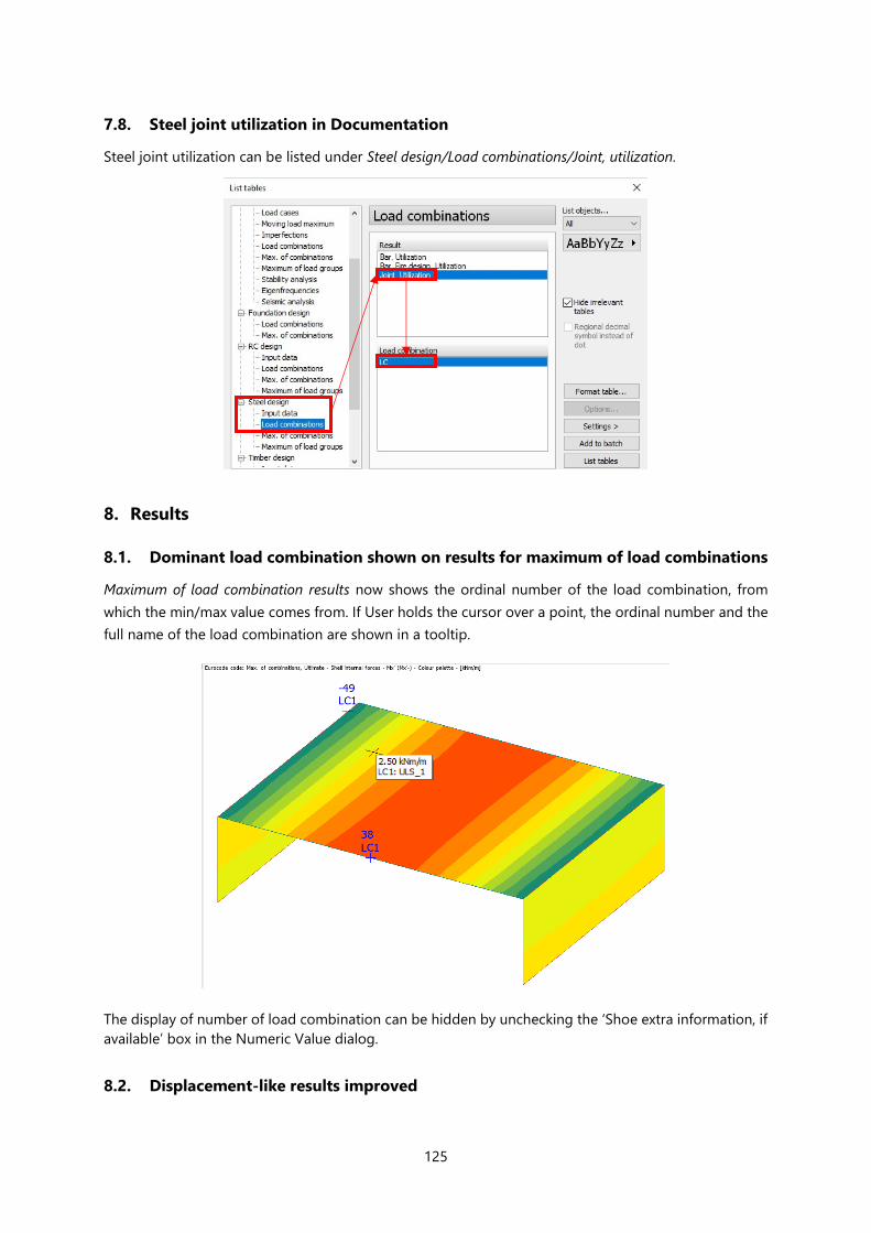
125
7.8. Steel joint utilization in Documentation
Steel joint utilization can be listed under Steel design/Load combinations/Joint, utilization.
8. Results
8.1. Dominant load combination shown on results for maximum of load combinations
Maximum of load combination results now shows the ordinal number of the load combination, from
which the min/max value comes from. If User holds the cursor over a point, the ordinal number and the
full name of the load combination are shown in a tooltip.
The display of number of load combination can be hidden by unchecking the ‘Shoe extra information, if
available’ box in the Numeric Value dialog.
8.2. Displacement-like results improved
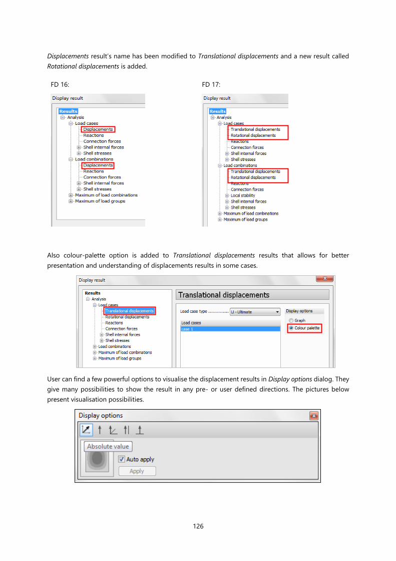
126
Displacements result’s name has been modified to Translational displacements and a new result called
Rotational displacements is added.
FD 16: FD 17:
Also colour-palette option is added to Translational displacements results that allows for better
presentation and understanding of displacements results in some cases.
User can find a few powerful options to visualise the displacement results in Display options dialog. They
give many possibilities to show the result in any pre- or user defined directions. The pictures below
present visualisation possibilities.

127
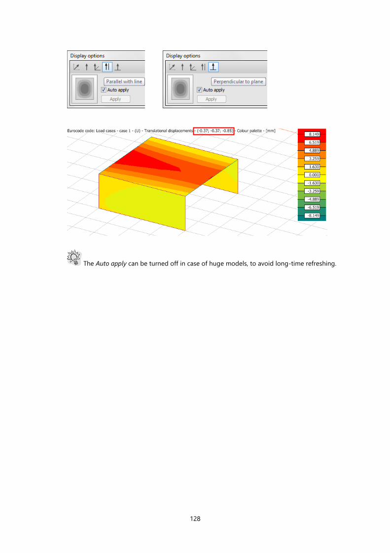
128
The Auto apply can be turned off in case of huge models, to avoid long-time refreshing.

129
8.3. Shear center result
In FD 17, the shear center can be displayed for every storey.
Each displayed shear center represents the result of a calculation based on the storeys
below that storey. For example, the calculation of the center displayed on “Storey 2” takes
also “Storey 1” and “Foundation” into account.
For displaying shear center, diaphragms are
needed for every storey.
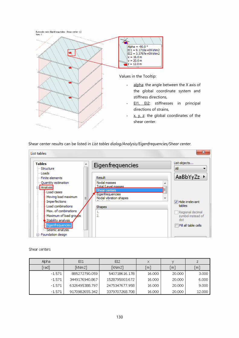
130
Shear center results can be listed in List tables dialog/Analysis/Eigenfrequencies/Shear center.
Values in the Tooltip:
- alpha: the angle between the X axis of
the global coordinate system and
stiffness directions,
- EI1, EI2: stiffnesses in principal
directions of strains,
- x, y, z: the global coordinates of the
shear center.

131
8.4. Mass result
In FEM-Design 17, Masses result is renamed to Nodal masses, and new result types: Nodal masses and
Total / Level masses are available,
Loads:
In FD 16:
In FD 17:

132
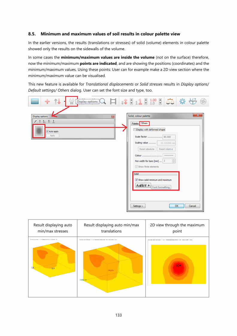
133
8.5. Minimum and maximum values of soil results in colour palette view
In the earlier versions, the results (translations or stresses) of solid (volume) elements in colour palette
showed only the results on the sidewalls of the volume.
In some cases the minimum/maximum values are inside the volume (not on the surface) therefore,
now the minimum/maximum points are indicated, and are showing the positions (coordinates) and the
minimum/maximum values. Using these points: User can for example make a 2D view section where the
minimum/maximum value can be visualised.
This new feature is available for Translational displacements or Solid stresses results in Display options/
Default settings/ Others dialog. User can set the font size and type, too.
Result displaying auto
min/max stresses
Result displaying auto min/max
translations
2D view through the maximum
point

134
8.6. Local stability results with more details
The maximum value and detailed calculation of the result is displayed.
The detailed calculation can be hidden by unchecking the ‘Show extra information, if available’ box in
the Numeric Value dialog.
8.7. Colours of principal stresses, moments and normal forces
Colouring of principal stress, moment and normal force results of shells has been modified to make the
result more clear. The algebraically larger value will be the first principal value, by default indicated
with green colour. The algebraically smaller value will be the second principal value, by default
indicated with red colour. Difference in the Display options dialogs and the results is shown on the
picture below.
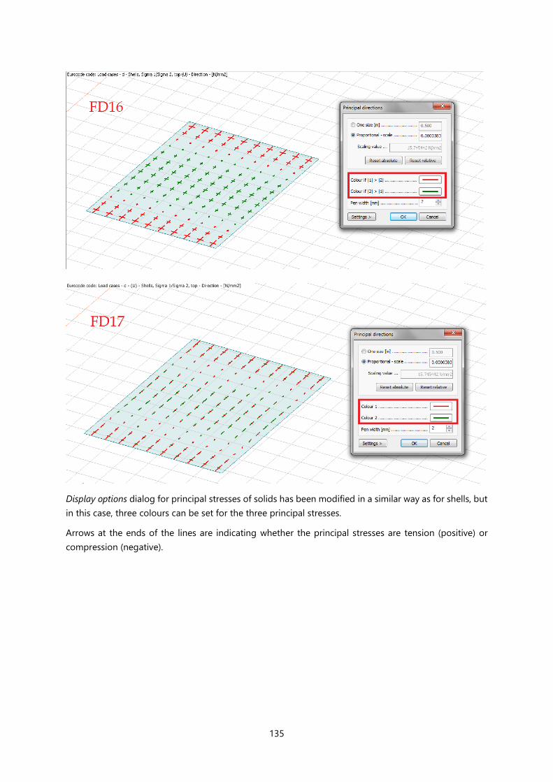
135
Display options dialog for principal stresses of solids has been modified in a similar way as for shells, but
in this case, three colours can be set for the three principal stresses.
Arrows at the ends of the lines are indicating whether the principal stresses are tension (positive) or
compression (negative).

136
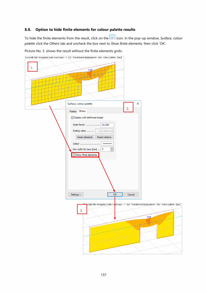
137
8.8. Option to hide finite elements for colour palette results
To hide the finite elements from the result, click on the icon. In the pop-up window, Surface, colour
palette click the Others tab and uncheck the box next to Show finite elements, then click ’OK’.
Picture No. 3. shows the result without the finite elements grids.
1.
2.
3.

138
8.9. Scale to view option for colour palette results
In FEM-Design 17 for results displayed by colour palette, a new option is available in the Display options
dialog. It automatically rescales the results considering the maximum and minimum values of the current
view.
With Scale to view option turned ON, if User hides part of the structure, the palette will be rescaled
automatically:
If the result to be displayed needs wider scaling than the customized has, the program
overwrites the scaling to the view.
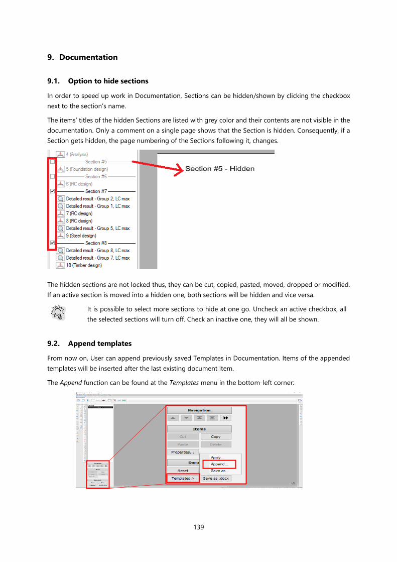
139
9. Documentation
9.1. Option to hide sections
In order to speed up work in Documentation, Sections can be hidden/shown by clicking the checkbox
next to the section’s name.
The items’ titles of the hidden Sections are listed with grey color and their contents are not visible in the
documentation. Only a comment on a single page shows that the Section is hidden. Consequently, if a
Section gets hidden, the page numbering of the Sections following it, changes.
The hidden sections are not locked thus, they can be cut, copied, pasted, moved, dropped or modified.
If an active section is moved into a hidden one, both sections will be hidden and vice versa.
It is possible to select more sections to hide at one go. Uncheck an active checkbox, all
the selected sections will turn off. Check an inactive one, they will all be shown.
9.2. Append templates
From now on, User can append previously saved Templates in Documentation. Items of the appended
templates will be inserted after the last existing document item.
The Append function can be found at the Templates menu in the bottom-left corner:

140
9.3. Docgraph windows are created according to the saved Window settings
User can save the Window settings for Docgraphs as default by clicking the Save as default button in the
Settings dialog.
Pictures 1 and 2 show that, if User turns off the grid but doesn’t save that setting as default, the next
inserted docgraph will be displayed as the first one was displayed originally.
If User saves the customized settings as default, every next inserted docgraph, will be displayed
according to the saved properties. (See picture 3. and 4.)
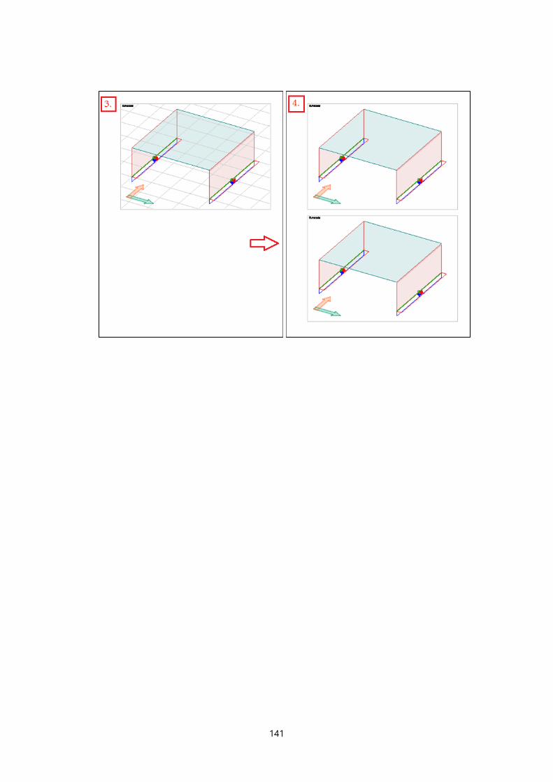
141

142
10. Others
10.1. FEM-Design Center
FEM-Design systray has been removed and replaced with a new, more informative tool called FEM-
Design Center. All the modules, useful links, updates and links to the add-ins are now in one place.
At the end of FEM-Design installation, user can select an option to launch the FEM-Design Center and
pin it to the taskbar for easier access, if necessary.
CTRL+Left mouse button will open the last model.
Shitf + Left mouse button will open history in a jumplist.
We highly suggest the User to pin the command center so right clicking the icon on the tray will open a
jumplist where all the modules are listed.

143
10.2. Drag and drop
In FEM-Design 17 “drag and drop” function is implemented. Files in all supported formats can be now
simply dragged and dropped to the FEM-Design.
Drag and drop

144
10.3. FEM-Design Support tool
This tool helps the User to reach the Support team easily and get answers for specific model dependant
questions. This can be found at Help/FEM-Design Support menu.
User can decide how to receive answer, via email or phone and/or TeamViewer (remote desktop
If the Attach current model is active, the current, saved model will be send to the support along with the
report. If the model includes linked DWG files, those files will be attached as well.
Add Files allows to add more files (e.g. pictures) to the report.
The Help button links to a guide on how to use this tool. There, one can find more detailed explanation
of the tool functionality and its limitation.

145
10.4. Company settings
It is a very fast way to export all FEM-Design settings and libraries to any other computer. With this
feature User can deliver their company preferences from one computer to another very easy and quickly.
.
Export and import settings can be found in the FEM-Design Center. The company settings file has
*.fdcs format.
Export Import
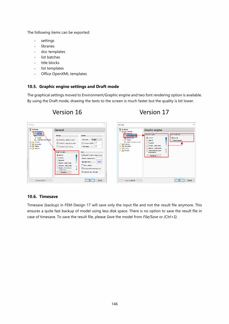
146
The following items can be exported:
- settings
- libraries
- doc templates
- list batches
- title blocks
- list templates
- Office OpenXML templates
10.5. Graphic engine settings and Draft mode
The graphical settings moved to Environment/Graphic engine and two font rendering option is available.
By using the Draft mode, drawing the texts to the screen is much faster but the quality is bit lower.
10.6. Timesave
Timesave (backup) in FEM-Design 17 will save only the input file and not the result file anymore. This
ensures a quite fast backup of model using less disk space. There is no option to save the result file in
case of timesave. To save the result file, please Save the model from File/Save or (Ctrl+S).
Version 16 Version 17