FCT/POSC/EIA/57671/2004

ABSES: Agent Based Simulation of Ecological Systems

Third Year Report

ABSES: Agent Based Simulation of Ecological

Systems

Luís Paulo Reis, Pedro Duarte, António Pereira

LIACC – Artificial Intelligence and Computer Science Laboratory

CIAGEB - Global Change, Energy, Environment and Bioengineering R & D Unit

FEUP – Faculty of Engineering of the University of Porto

UFP - University Fernando Pessoa, Porto

March of 2008

2

Table of Contents

ABSTRACT ........................................................................................................................................................... 5

1 INTRODUCTION ....................................................................................................................................... 7

2 CASE STUDIES ......................................................................................................................................... 10

2.1 CARLINGFORD LOUGH ........................................................................................................................ 10

2.2 SUNGO BAY ........................................................................................................................................ 11

2.3 RIA FORMOSA LAGOON ...................................................................................................................... 12

3 DATA AND MODEL GATHERING ....................................................................................................... 14

4 MULTI-AGENT SIMULATION SYSTEM ............................................................................................ 17

5 ECODYNAMO – ECOLOGICAL SIMULATOR DEVELOPMENT ................................................. 19

6 ECOLANG – DEVELOPMENT OF AN ECOLOGICAL MODELLING LANGUAGE................... 22

7 INTELLIGENT AGENT DEVELOPMENT .......................................................................................... 24

8 SEASHELL FARMER AGENT DEVELOPMENT ............................................................................... 31

8.1 SHEASHELL FARMING AGENT ............................................................................................................. 31

8.2 ALGORITHM IMPLEMENTATION ........................................................................................................... 32

8.3 TACTICS SYSTEM ................................................................................................................................ 35

8.4 OPTIMIZATION RESULTS ..................................................................................................................... 36

9 CONCLUSIONS AND FUTURE WORK ............................................................................................... 38

REFERENCES .................................................................................................................................................... 40

3

List of Figures

Figure 1: Carlingford Lough, showing the oyster cultivation areas and compartments used in

the model of Ferreira et al [Ferreira et al., 1998]. .................................................................. 11

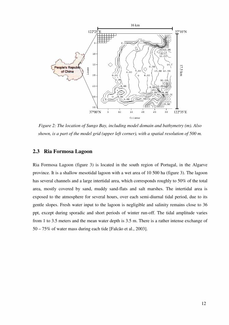
Figure 2: The location of Sungo Bay, including model domain and bathymetry (m). Also

shown, is a part of the model grid (upper left corner), with a spatial resolution of 500 m. .... 12

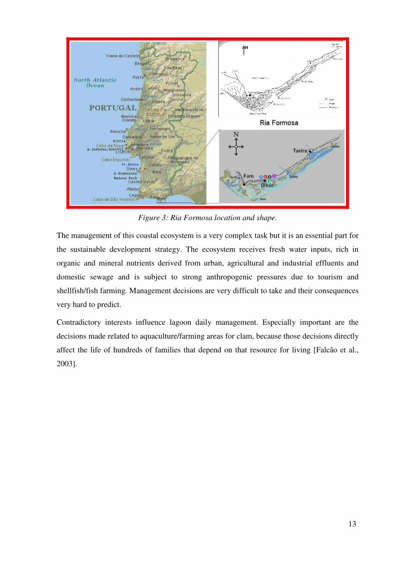
Figure 3: Ria Formosa location and shape.............................................................................. 13

Figure 4: Layout of the Carlingford Lough model. .................................................................. 14

Figure 5: Layout of the Sungo Bay model. ............................................................................... 15

Figure 6: Layout of Ria Formosa (Algarve) model .................................................................. 16

Figure 7: System Architecture (adapted from [Pereira et al., 2004]) .................................... 17

Figure 8: Experimental system for the different pieces of software [Pereira et al., 2005] ..... 18

Figure 9: EcoDynamo main window [Pereira & Duarte, 2005] ............................................. 20

Figure 10: 2D window of the development agent with farming areas visible ......................... 24

Figure 11: Farming areas and benthic species visible ............................................................ 24

Figure 12: Zoom option in the first level .................................................................................. 25

Figure 13: Farming areas and benthic species zoomed ......................................................... 25

Figure 14: Available commands from development agent ...................................................... 26

Figure 15: Classes Available from model ................................................................................ 26

Figure 16: Get Variables from TRiaF2DPhytoplankton class ................................................. 27

Figure 17: Get variable value .................................................................................................. 28

Figure 18: Set variable value ................................................................................................... 28

Figure 19: Get parameters from one class ............................................................................... 29

Figure 20: Select variables from model ................................................................................... 29

Figure 21: Selecting variables (second phase) ........................................................................ 30

Figure 21: Two different configurations of farming areas: five farming areas are selected

from the wide available area in each example. ........................................................................ 32

4

List of Tables

Table 1: EcoDynamo class names and simulated variables .................................................... 21

Table 2: Results of the tactics tested ........................................................................................ 36

Table 2: Best solutions achieved .............................................................................................. 37

Abstract

This report presents the research developed during the first three civil years of project

ABSES: Agent Based Simulation of Ecological Systems (FCT/POSC/EIA/57671/2004).

During this period the project predicted chronogram was followed with about six months of

delay and thus this period of delay was asked to FCT in order for the project to be completed.

The delay was mainly on some of the final tasks, due to some difficulty in contracting

qualified manpower for scholarships and services and concluding the final experiments.

In the first two civil years of ABSES the following tasks were completed:

• Data and model data gathering for three different ecosystems (Carlingford Lough,

Sungo Bay, and Ria Formosa Lagoon).

• Development of a multi-agent simulation system for ecological simulations;

• Development of a realistic ecological simulator – EcoDynamo integrated on the multi-

agent simulation system.

• Development of a visualization system for the ecological simulations enabling simple

visualization and analysis of the simulations executed.

• Development of an ecological modelling language – ECOLANG –and its integration

in the simulation system, enabling high-level communication of all the simulation

system applications.

• Development of one special software component (TECDPForm) to facilitate the

integration of any new agent or application in the simulation system. This component

is composed by four fundamental components: one complete multi-threaded TCP

server, one complete TCP client, one cyclic timer for communications control and one

multiline edit control for display messages received and transmitted. All applications

that belong to the EcoSimNet must include one component that inherits from

TECDPForm (it is used for as an ancestor class for ECOLANG specific protocol

implementation).

• Development of a simple calibration agent, capable of calibrating the simulation

models. This calibration agent that intends to optimise the fit between observed and

simulated results.

• Development of simple aquaculture agents capable of interacting with the simulation

system and perform seeding and harvesting operations of bivalves.

6

In the third year, more complex aquaculture agents were developed capable of optimizing the

production of distinct bivalves in a realistic costal ecosystem. First experiments were

performed with Sungo Bay model, due to its simplicity when compared with Ria Formosa

model, to validate the approach. A more elaborated visualization system was also developed

enabling attractive visualization and better analysis of the simulations executed. The

development of aquaculture agents was continued and finalized. Aquaculture agents were

developed capable of not only optimizing bivalve’s production in the aquatic systems but also

optimizing more complex evaluation functions, including not only the production, the water

quality and phytoplankton concentration. The aquaculture agents developed were tested in the

simulation system, using Sungo Bay scenarios for optimizing bivalves production in the

aquatic systems and optimize other more elaborated evaluation functions.

The Multi-Agent Simulation System developed enables decision-makers and stakeholders in

the ecological system simulation to be modelled as intelligent agents that communicate using

ECOLANG with the simulation tool (EcoDynamo) building a multi-agent community system.

The intelligent agents, each one with some goals about the simulation results of the simulated

system, have perception of their environment, reason, using their knowledge and are able to

change the simulated environment by using a given set of configurable actions.

During 2008, experiments are being performed with the calibration agent and aquaculture

agents developed and the EcoDynamo simulator system, using the coastal system's models

previously developed. These experiments will enable to validate the complete system and

further validate the agent-based methodologies developed.

7

1 Introduction

Coastal lagoons always performed an important role in the life of the human beings. They

represent a small part of the area and volume of the oceans but, because they are the interface

between land and sea, they allow an enormous amount of possible activities for work and

leisure and guarantee several basic services to humanity.

In the last century, human population migrates intensively from inland to coastal boundaries

and, nowadays, at least 60% of the human population lives within 60km from the sea [Duarte

et al. 2007a]. In recent decades, after the observation of some ecological disasters, scientists

and stakeholders become aware that they must work together to ensure the appropriate

management of those areas in order to maintain the overall quality of the ecosystems

compatible with development strategies – that’s what is commonly called ecosystem

management for sustained development.

Aquaculture, touristic and harbour activities, urban development and human leisure converge

to the coastal ecosystems, forcing loads of fresh water inputs, rich in organic and mineral

nutrients derived from agricultural, urban and industrial effluents and domestic sewage

[Duarte et al. 2007b].

The sustainable development strategies for these ecosystems must include all the known

interests in each region and should explain, undoubtedly, why some decisions must be taken

and the benefits achieved in the medium or long term for each ecosystem. These strategies

may include targets for short-term (when the ecosystem threats with immediate collapse in

terms of ecological balance), but should be designed for future generations. The inclusion of

the system stakeholders’ in the decision-making process is crucial to ensure the commitment

of the population to the decisions taken even if their consequences may have some immediate

negative effect on the day life of each one.

The use of simulation and ecological models is becoming a widespread tool in the

management of coastal ecological systems towards a sustainable development strategy.

Therefore, it is important to integrate in the models the human reasoning, decisions and

actions over the ecological systems. This task is very hard to include and none of the

traditional simulation processes and models include “human behaviour” because it is not easy

to predict, even if the human decisions are limited by legal regulations and laws.

The fragmented legal framing of the administration responsibilities facilitates an overlap of

abilities between two or more entities, leaving simple questions like: “Is it advisable to

8

enlarge an opened navigation channel (due to tourism pressure and boat navigation

demands)?” without an immediate answer. A positive answer to the previous question raises

another complex one: “What will be the future consequences and/or benefits?”

The huge number of possible combinations, generated by the different management decisions

and options, the opposite interests of the stakeholders and the institutional authorities, and the

slowness of the decision processes, increases the difficulty to implement automatic real-time

management policies [Pereira et al. 2007].

There has been a significant increase in the usage of mathematical models across almost all

fields of science over the last decades, certainly related to the rapid progresses in hardware

and software development. Models are now intensively used in theoretic and applied Ecology.

Recently, a new field of research has been emerging from the linkage of Artificial Intelligence

(AI) techniques like Machine Learning (ML) and Autonomous Agents with Environmental

Sciences, as reflected in several international workshops.

After a model is implemented, the first round of simulations is generally designed to test its

internal logic against common sense knowledge. Once this task is accomplished, it is

necessary to calibrate the model, i.e., to perform a second round of simulations and to tune

model parameters in order to reproduce observed data. In every mathematical model,

parameters regulate the behaviour of equations describing temporal and spatial changes of

model state variables and their interactions.

Generally, there is some uncertainty associated with each parameter. This “tuning” procedure

is a hard and “tedious” work requiring a good understanding of the effects of different

parameters over the available variables. A third round of simulations is generally performed

to validate the model, i.e., to compare predicted with observed results that were not used in

the calibration process. Once the model is validated it may be used as a predictive tool and

simulations may be set up depending on the purposes for which it was developed. When the

goal is to find some optimal solutions, a large number of trial and error simulations may be

required.

Some of the learning processes associated with model implementation may be automated to

save man power and increase the performance of some tasks, such as model calibration and

search for optimum solutions. Automatic calibration procedures already exist, based on

systematic and exhaustive generation of parameter vectors and using several convergence

methods. However, they require a large number of model runs and are, therefore, not

applicable to complex ecosystem models demanding large computational times. A possible

9

alternative may be to develop a self-learning tool that simulates the learning process of the

modeller about the simulated system. A similar approach may be used to find optimal

solutions to environmental problems. In both cases, Autonomous Agents may be a sound way

to implement the self-learning tools. Autonomous Agents also enable to introduce in the

simulations, in a very natural way, the human element, whose reasoning process is very

difficult to model by traditional simulation processes.

This project aimed at developing a complete ecosystem multi-agent simulation system,

including a realistic ecological simulator, a calibration agent based on machine learning

techniques capable of calibrating complex ecological models, autonomous agents representing

the intelligent entities present in the simulation capable of performing aquaculture operations

in the developed simulation system and a specific language enabling the communication

between all the system applications.

The simulation system is applied to several ecological models of coastal ecosystems

developed for the project, including Sungo Bay (in China), Ria Formosa Lagoon (in Algarve)

and Carlingford Lough (Ireland and Northern Ireland). The simulation system may be used

for aquaculture optimization and simulating the effects of several types of changes in the

ecosystem at short and long term.

The rest of the report is organized as follows. Section 2 describes the three case studies

selected for this project (Carlingford Lough, Sungo Bay and Ria Formosa) and section 3

describes the data and model gathering process used. Section 4 briefly describes the multi-

agent simulation system developed while the next sections describe the ecological simulator .

EcoDynamo (section 5) and the communication language – ECOLANG – used between all

the system applications (section 6). Section 7 presents an overview of the agent development

process used. Section 8 analyses in more detail the development of specific agents with

emphasis on the seashell farming agent. Section 9 presents detailed project conclusions and

future work.

10

2 Case studies

Three case studies were selected for this project: Carlingford Lough (Ireland), Sungo Bay

(People’s Republic of China) and Ria Formosa (Portugal) – representing three coastal

ecosystems where aquaculture is a relatively important economic activity, for which

mathematical models were already developed in former European union projects, with the

participation of some of the researchers involved in the current project:

(i) Development of an ecological model for mollusc rearing areas in Ireland and

Greece - Program FAR/CEE (finished in 1994);

(ii) Carrying capacity assessment and impact of aquaculture in Chinese bays -

Program INCO – UE, contract nº: ERB IC18 – CT98 – 0291 (finished in 2002).

(iii) DITTY – Development of information technology tools for the management of

Southern European coastal lagoons under the influence of river runoff, EESD

Project EVK3-CT-2002-00084 (finished in 2006).

Another common feature of these ecosystems is that implemented models were designed to

help optimising bivalve aquaculture. Accumulated experience shows that this optimization is

a very complex problem depending, among other things, on the way aquaculture areas are

distributed in space and suggesting that there is no one optimum solution, but a “family” of

good solutions. In fact, this complexity was one of the motivations for the current project.

2.1 Carlingford Lough

Carlingford Lough is a small embayment on the Irish east coast, forming part of the border

between the Republic of Ireland and Northern Ireland (figure 1). It is 16.5 km long and 5.5

km wide at its widest point, with an area of approximately 40 km2 and an average depth of 5

m. The mean tidal prism corresponds to about 50% of the mean Lough volume. It has

important intertidal areas in the north and south margins that correspond to almost half of the

total area. The main freshwater discharge is from the Newry (Clanrye) river, with a small flow

rate that can vary from 1 m3s-1 in Summer to 9 m3s-1 in Winter (roughly 105-106 m3d-1).

This ecosystem as become a oyster cultivation area. An estimate of its carrying capacity for

oyster culture was obtained by Ferreira et al. [Ferreira et al. 1998].

11

N

Carlingford

NorthernIreland

IrelandRiver Newry (Clanrye)

3 km

Box 1 Box 2 Box 3

Intertidal area Oyster areas Model boxes

Irish Sea

Figure 1: Carlingford Lough, showing the oyster cultivation areas and compartments used in

the model of Ferreira et al [Ferreira et al., 1998].

2.2 Sungo Bay

Sungo bay is located in Shandong province of People’s Republic of China (Fig. 2). With an

area of 180 km2 and depths varying gradually until approximately 20 m at the sea boundary

(figure 2), it has been used for aquaculture for more than 20 years [Guo et al., 1999]. The

main cultivated species include kelp (Laminaria japonica), oyster (Crassostrea gigas) and

scallop (Chlamys farreri). Scallops and oysters are mostly contained in lantern nets and kelps

are tied to ropes. One of the most limiting factors for bivalve culture in Sungo bay is scallop

mortality. High summer mortalities in recent years have led to changed aquaculture practices,

including shifting the rearing periods.

12

16 km

17

.5 k

m

122º35’E

122º25’E

37º00’N

37º10’N

Figure 2: The location of Sungo Bay, including model domain and bathymetry (m). Also

shown, is a part of the model grid (upper left corner), with a spatial resolution of 500 m.

2.3 Ria Formosa Lagoon

Ria Formosa Lagoon (figure 3) is located in the south region of Portugal, in the Algarve

province. It is a shallow mesotidal lagoon with a wet area of 10 500 ha (figure 3). The lagoon

has several channels and a large intertidal area, which corresponds roughly to 50% of the total

area, mostly covered by sand, muddy sand-flats and salt marshes. The intertidal area is

exposed to the atmosphere for several hours, over each semi-diurnal tidal period, due to its

gentle slopes. Fresh water input to the lagoon is negligible and salinity remains close to 36

ppt, except during sporadic and short periods of winter run-off. The tidal amplitude varies

from 1 to 3.5 meters and the mean water depth is 3.5 m. There is a rather intense exchange of

50 – 75% of water mass during each tide [Falcão et al., 2003].

13

Figure 3: Ria Formosa location and shape.

The management of this coastal ecosystem is a very complex task but it is an essential part for

the sustainable development strategy. The ecosystem receives fresh water inputs, rich in

organic and mineral nutrients derived from urban, agricultural and industrial effluents and

domestic sewage and is subject to strong anthropogenic pressures due to tourism and

shellfish/fish farming. Management decisions are very difficult to take and their consequences

very hard to predict.

Contradictory interests influence lagoon daily management. Especially important are the

decisions made related to aquaculture/farming areas for clam, because those decisions directly

affect the life of hundreds of families that depend on that resource for living [Falcão et al.,

2003].

14

3 Data and Model Gathering

The main objective of this task was to synthesise available data and implement/improve

models already developed for different ecosystems. Priority was given to case studies where

elements of the project team participated and that have been published in specialized literature

– the ecological models for Carlingford Lough (Ireland) [Ferreira et al., 1998], for Sungo Bay

(People’s Republic of China) [Duarte et al., 2003] and Ria Formosa (Algarve) [Duarte et al,

2006a] [Duarte et al. 2006b]. All data necessary to initialize and parameterise these models is

available to the authors of this project, from the above mentioned references, from local

providers at Ria Formosa, and from databases produced during several projects, where

members of the research team took part.

These models were implemented with the modelling software described below – EcoDynamo

(cf. – 4.). Some improvements were included based on previous experience. For example, the

Carlingford model was implemented as a coupled physical-biogeochemical model instead of a

box model following the approach described in [Duarte et al., 2003]. A spatial staggered grid

[Vreugdenhil, 1989] was used for each model with a resolution of 356, 500 and 100 m and a

total of c.a. 900, 1120 and 132540 cells, for the Carlingford, the Sungo and the Ria Formosa

models, respectively. At each time step, gain and loss processes are computed for all model

state variables.

N

Carlingford

NorthernIreland

IrelandRiver Newry (Clanrye)

3 km

Box 1Box 2 Box 3

Intertidal area Oyster areas Model boxes

Irish Sea

N

Carlingford

NorthernIreland

IrelandRiver Newry (Clanrye)

3 km

Box 1Box 2 Box 3

Intertidal area Oyster areas Model boxes

Irish Sea

ms-1

Figure 4: Layout of the Carlingford Lough model.

15

Hydrodynamic processes are explicitly simulated using the equations described in [Duarte et

al., 2003]. The resulting current velocity fields at each model time step are used to calculate

transport of all dissolved and particulate water properties, such as nutrient concentrations,

suspended matter, phyto- and zooplankton. Also, the growth of cultivated species (bivalves

and kelps) is computed for all aquaculture areas. The general layout of the models is shown

together with some result outputs in figures 4 - 6. These models are being used as case studies

to run and test the Multi-Agent Simulation System (cf. – 3). Currently, simulations are being

carried out with different aquaculture scenarios (e.g. virtual creation of new aquaculture areas

or redistribution of existing ones) with the objective of maximizing production. These

simulations are controlled by a “farmer” intelligent agent described below (cf. – 7).

Figure 4 displays the location of Carlinford Lough in Ireland – an oyster rearing area. The

bottom left panel of figure shows the bathymetry and the bottom right panel displays a

velocity field calculated by the model during the ebb.

mg m-3m s-1

Figure 5: Layout of the Sungo Bay model.

Figure 5 displays the characteristics of Sungo Bay in China. The upper left figure shows the

location of Sungo Bay. The upper right panel shows the location of oyster, clams and kelps

16

(dark green) aquaculture areas. The bottom left panel shows an example of a current velocity

field calculated by the model and the bottom right panel shows an example of simulated

chlorophyll concentration (a surrogate for phytoplankton biomass – one of the major bivalve

food items).

-1

Flood Flood

Tavira-Cabanas

Tavira-Clube Naval

Fuzeta-Canal

Olhão –

Canal de Marim

Faro-Harbour

Ancão

Olhão

Faro –

main channel

m s-1

Figure 6: Layout of Ria Formosa (Algarve) model

Figure 6 shows Ria Formosa in Portugal and stations used for model validation. The bottom

panel shows an example of a current velocity field calculated by the model.

17

4 Multi-Agent Simulation System

During the first year of ABSES project a complete architecture for a multi-agent simulation

system for ecological simulations was developed. The architecture proposed here for the

simulation system (figure 7) is based on the use of Intelligent Agents” [Weiss, 1999],

[Wooldridge, 2002], [Norvig and Russel, 2003], [Reis, 2003] to represent system entities in

the context of a multi-agent system.

Each intelligent entity involved with the ecological system is included in the simulation

system as an agent (Natural Park Directorate Agent, Shellfish Farmer Agent, Official Tourism

Manager Agent, City Council Agent, Navy Command Agent …). Any action planned by the

agents that influences the ecosystem is previously communicated to the model database; the

simulation system runs and the results are presented to a decision support system to help

managers’ decisions [Pereira et al., 2004].

Figure 7: System Architecture (adapted from [Pereira et al., 2004])

18

All the communications between entities are done using ECOLANG [Pereira et al., 2005] - a

communication language developed especially for this project and acting as a common

framework to exchange information between the software applications.

Although each application has its own user interface, the user can access the different

components’ information via the visualisation system, a common entry for the system.

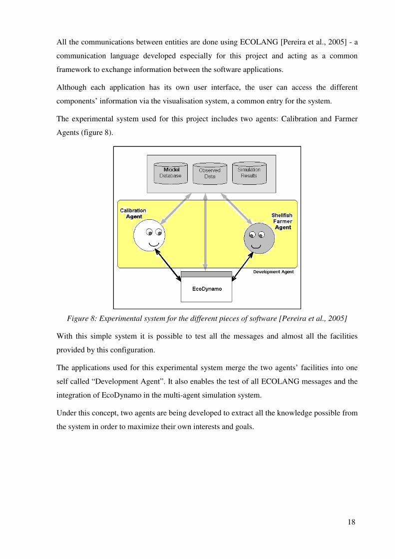
The experimental system used for this project includes two agents: Calibration and Farmer

Agents (figure 8).

Figure 8: Experimental system for the different pieces of software [Pereira et al., 2005]

With this simple system it is possible to test all the messages and almost all the facilities

provided by this configuration.

The applications used for this experimental system merge the two agents’ facilities into one

self called “Development Agent”. It also enables the test of all ECOLANG messages and the

integration of EcoDynamo in the multi-agent simulation system.

Under this concept, two agents are being developed to extract all the knowledge possible from

the system in order to maximize their own interests and goals.

19

5 EcoDynamo – Ecological Simulator Development

The main expected result from this task was to finalise an user-friendly simulation software

enabling the simulation of aquatic ecosystems and to implement it to some case studies. The

software (initially called EcoDyn, hereafter referred as EcoDynamo – Ecological Dynamics

Model) was partially developed within the scope of the European project DITTY

(www.dittyproject.org). It has been further developed to accommodate several functionalities,

such as a communication interface with intelligent agents using ECOLANG – A

communication language for simulations of complex ecological systems [Pereira et al., 2005]

(cf. – 5).

EcoDynamo (figure 9) is an object-oriented software for hydrodynamic and biogeochemical

modelling of aquatic ecosystems. The source code is written in C++. It consists of a “shell” in

an windows environment to manage the graphical interface, the communication between the

user and several output devices and between the various objects (or classes) that simulate

ecosystem processes.

Different classes simulate different variables and processes, with proper parameter and

process equations (table 1). Classes can be selected or deselected from shell dialogs

determining its inclusion or exclusion in each simulation run of the model.

The simulated processes include:

• Hydrodynamics of aquatic systems: current speeds and directions;

• Thermodynamics: energy balances between water and atmosphere and water

temperature;

• Biogeochemistry: nutrient and biological species dynamics;

• Anthropogenic pressures, such as biomass harvesting.

The ecosystem characteristic properties are described in a model database (Configuration

Files): morphology - geometric representation of the model, dimensions, number of cells -

classes, variables, parameter initial values and ranges.

The communication between different objects representing different variables and processes

is made through the shell. This allows keeping a logbook of the interactions between different

objects which is an important tool in the machine-learning process referred below (cf. – 7).

20

Simulation activity can be followed with the help of log files, activated previously before each

simulation run.

The user can choose between file, chart or table to store the simulation results. These output

formats are compatible with some commercial software (like MatLab®

) products, enabling

their posterior treatment.

Figure 9: EcoDynamo main window [Pereira & Duarte, 2005]

This application has an interface module (implementing the EcoDynamo Protocol) that

enables communications with other programs for external control. For example, the

simulations can be controlled by commands such as start / stop / pause / step.

Each class is contained in one DLL (Dynamic Link Library) that is included in the application

package. This approach enables the inclusion of new classes without the need of rebuilding all

the software.

21

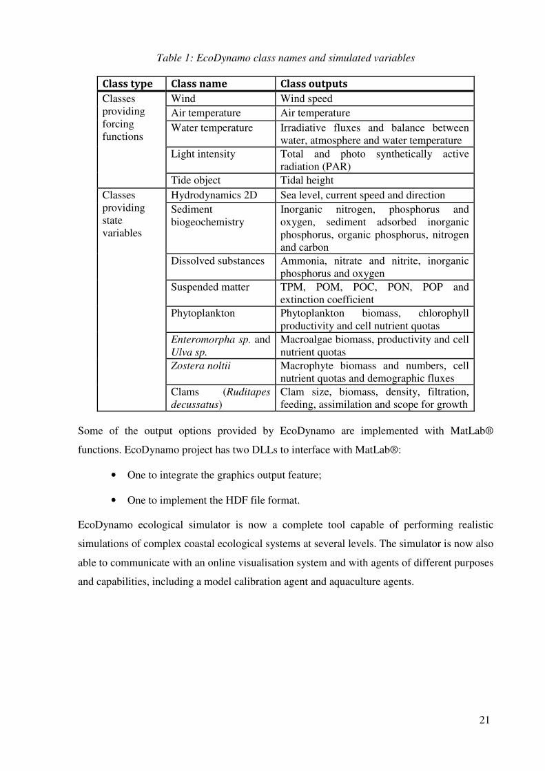
Table 1: EcoDynamo class names and simulated variables

Class type Class name Class outputs

Classes

providing

forcing

functions

Wind Wind speed

Air temperature Air temperature

Water temperature Irradiative fluxes and balance between

water, atmosphere and water temperature

Light intensity Total and photo synthetically active

radiation (PAR)

Tide object Tidal height

Classes

providing

state

variables

Hydrodynamics 2D Sea level, current speed and direction

Sediment

biogeochemistry

Inorganic nitrogen, phosphorus and

oxygen, sediment adsorbed inorganic

phosphorus, organic phosphorus, nitrogen

and carbon

Dissolved substances Ammonia, nitrate and nitrite, inorganic

phosphorus and oxygen

Suspended matter TPM, POM, POC, PON, POP and

extinction coefficient

Phytoplankton Phytoplankton biomass, chlorophyll

productivity and cell nutrient quotas

Enteromorpha sp. and

Ulva sp.

Macroalgae biomass, productivity and cell

nutrient quotas

Zostera noltii Macrophyte biomass and numbers, cell

nutrient quotas and demographic fluxes

Clams (Ruditapes

decussatus)

Clam size, biomass, density, filtration,

feeding, assimilation and scope for growth

Some of the output options provided by EcoDynamo are implemented with MatLab®

functions. EcoDynamo project has two DLLs to interface with MatLab®:

• One to integrate the graphics output feature;

• One to implement the HDF file format.

EcoDynamo ecological simulator is now a complete tool capable of performing realistic

simulations of complex coastal ecological systems at several levels. The simulator is now also

able to communicate with an online visualisation system and with agents of different purposes

and capabilities, including a model calibration agent and aquaculture agents.

22

6 ECOLANG – Development of an Ecological

Modelling Language

ECOLANG [Pereira et al., 2005] was developed with the purpose of exchange information

between one simulation application of aquatic ecosystems and external agents. It is a high-

level language capable of describing ecological systems in terms of regional characteristics,

living agent’s perceptions and actions and is independent from any hardware or software

platform.

ECOLANG development was based on COACH UNILANG work from Reis and Lau [Reis

and Lau, 2002]. This language, along with a specific communication protocol, will enable the

agents in the multi-agent system to understand each other in the ecological domain. Some pre-

requisites were enounced before its development:

• It must be a high-level language understood by software agents and by humans;

• It must have simple syntax validation;

• Its ontology must be oriented to aquatic systems;

• It must be easily adaptable to new actors included in the system;

• It must be independent from any hardware or software platform, including operating

system or programming language.

ECOLANG messages describe regional characteristics of the ecological systems, translate

agents’ actions and perceptions and enable different levels of communication:

• Execution: commands over the simulation model (run, stop, pause…);

• Configuration: select sub-domain, select classes, change variables and parameters’

initial values, choose which variables output, simulation period and time step before

the model runs;

• Definitions: aggregate cells into named regions according to some common

properties, define sub-domains based in the named regions;

• Statistics: collect results from simulation experiments, either online or offline

operation, compare results with previous simulation experiments or observed data and

advise the configuration module the expected actions to take;

23

• Events: spontaneous messages that agents generate to inform some important events

or results.

Message definitions used by ECOLANG follow the BNF formalism. Backus-Naur Form

(BNF) is the best-known meta-language (a language used for describing languages) in the

field of computer science. It was invented by John Backus and Peter Naur [Naur, 1960] to

describe the syntax of Algol 60 in an unambiguous manner. ECOLANG notation is an

extension to the original BNF formalism adding the following meta-symbols:

{ } used for repetitive items (one or more times);

[ ] encloses types of values;

Terminal symbols use bold face letters.

The basic message structure is:

<MESSAGE> ::= message (<ID> <SENDER> <RECEIVER> <MSG_CONTENT>)

<ID> ::= [integer]

<SENDER> ::= [string]

<RECEIVER> ::= [string]

<MSG_CONTENT> ::= <DEFINITION_MSG> | <ACTION_MSG> |

<PERCEPTION_MSG> | <CONNECTION_MSG>

Where <ID> is the identifier of the message sent by sender (it’s managed by each agent that

defines its own numbering system); <SENDER> is the name of the agent that sends the message;

<RECEIVER> is the name of the agent target of the message and <MSG_CONTENT> is the body of

the message with the relevant information.

Messages can be from four basic types: definitions, actions, perceptions and connection.

Definitions and connection messages are generic (used by anyone of the communication

partners); actions and perceptions are specific to each kind of agents involved in the system.

Connection messages are used to identify host computer and server port used in the

communication and must precede the dialog between applications.

For example, one message defining one region could be:

message (3 Develop_Agent EcoDynamo define(Kelp_1 intertidal

excellent (sandy excellent)(rect(point 21 27)(point 17 15))

(rect(point 1 1)(point(10 15)))

A complete description of the language’s syntax and examples may be found in [Pereira et al.,

2005].

24

7 Intelligent Agent Development

In order to test the multi-agent simulation system, a simple agent (Development Agent) was

developed and integrated in the experimental system. The agent has some graphical facilities

that will also be available in the visualisation application in order to facilitate the simulation

system testing and debugging process. With this agent the user can test all the messages

defined in the EcoDynamo protocol following the ECOLANG specification.

Figure 10: 2D window of the development agent with farming areas visible

Figure 11: Farming areas and benthic species visible

Its manipulation is very intuitive. The user must select the desired model enabling the “World

View” window. The morphology of the modelled system and the configured bivalves and

benthic species’ implantation areas are read. The user can see one 2D image of the model’s

25

domain with the areas of bivalves and benthic species implantation represented in different

colours (figures 10 and 11).

When the domain of the model is large (like Ria Formosa) it is difficult for the user to see

clearly individual cells and to define particular regions. One zoom option was included in the

application (figure 12) for readability of the model domain. This option can be applied

consecutively to produce a better visualisation of the model domain.

Figure 12: Zoom option in the first level

Zooming in several times can produce a display like the one showed in figure 13. With this

image the user can interact more accurately with the simulation model.

Figure 13: Farming areas and benthic species zoomed

Application menus enable the user to act over EcoDynamo. Figure 14 shows some of the

Development Agent menus and submenus.

26

Figure 14: Available commands from development agent

For instance, if the user wants to know what the available classes are configured in the model,

it selects the command “Classes Available” in the Specifications menu. Figure 15 shows one

example of the command and the result window. The command is translated to the

corresponding ECOLANG message and sent to the EcoDynamo application; EcoDynamo

answers with the names of the available classes in another message; the result is shown in the

“Classes Available” window.

Figure 15: Classes Available from model

The user can also see the variables existent in each class: selecting the “Get Variables…”

command from the Specifications menu; the result is shown in figure 16. In this figure the

Development Agent main window is also visible; in this window all the messages, sent and

27

received, are logged. This enables the user to follow the messages exchanged between the

applications.

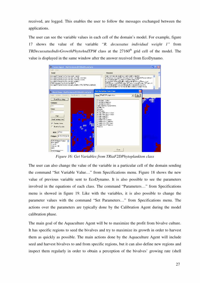
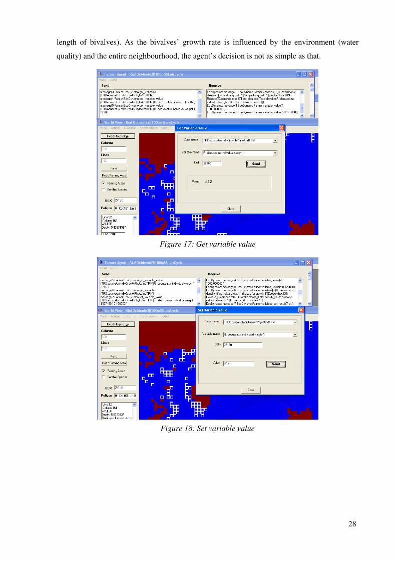
The user can see the variable values in each cell of the domain’s model. For example, figure

17 shows the value of the variable “R. decussatus individual weight 1” from

TRDecussatusIndivGrowthPhytoAndTPM class at the 27160th

grid cell of the model. The

value is displayed in the same window after the answer received from EcoDynamo.

Figure 16: Get Variables from TRiaF2DPhytoplankton class

The user can also change the value of the variable in a particular cell of the domain sending

the command “Set Variable Value…” from Specifications menu. Figure 18 shows the new

value of previous variable sent to EcoDynamo. It is also possible to see the parameters

involved in the equations of each class. The command “Parameters…” from Specifications

menu is showed in figure 19. Like with the variables, it is also possible to change the

parameter values with the command “Set Parameters…” from Specifications menu. The

actions over the parameters are typically done by the Calibration Agent during the model

calibration phase.

The main goal of the Aquaculture Agent will be to maximize the profit from bivalve culture.

It has specific regions to seed the bivalves and try to maximize its growth in order to harvest

them as quickly as possible. The main actions done by the Aquaculture Agent will include

seed and harvest bivalves to and from specific regions, but it can also define new regions and

inspect them regularly in order to obtain a perception of the bivalves’ growing rate (shell

28

length of bivalves). As the bivalves’ growth rate is influenced by the environment (water

quality) and the entire neighbourhood, the agent’s decision is not as simple as that.

Figure 17: Get variable value

Figure 18: Set variable value

29

Figure 19: Get parameters from one class

The agent can select variables related with the environment (all model simulated variables are

available), collect their values (total or medium) and relate them with some kind of qualitative

importance to rank the options assumed.

Figure 20: Select variables from model

30

Each change in the cultivation area of bivalves, or in their density distribution, will generate a

new scenario. Each run of the model with different configuration of the site generates

different results that must be saved to posterior analysis.

Figure 20 shows one example of variables selection from one simulation run. The selection

must be done before the simulation. After clicking on the “Select Variables” button, another

window pops-up (figure 21) to specify which of the variables will be time integrated. In this

dialog, the user (in this case the aquaculture farmer) can choose from which regions the

variable values will be collected.

Figure 21: Selecting variables (second phase)

The development of this simple agent enabled us to test and validate the multi-agent

simulation system, the models developed and the ecological simulator application. It also

enabled to fine tune ECOLANG that will evolve in a near future to a new version including

the experience gained by its first real application.

31

8 Seashell Farmer Agent Development

The development of agents with capabilities to interact in an intelligent manner with the

Multi-Agent simulation system is one of the main originalities of ABSES projects. Thus,

several distinct types of agents were developed capable of interacting with the simulator,

including agents with optimization capabilities capable of Seashell farming optimization

[Cruz, 2006] [Cruz et al., 2007] and several other agents capable of generic optimization of

dynamic scenarios [Restivo, 2006] [Restivo & Reis, 2006], simple agents with emotional

capabilities [Barteneva et al., 2006], [Barteneva et al., 2007] and a calibration agent for

ecological simulations [Valente et al., 2008]. The rest of this section describes in more detail

the seashell farmer agent developed capable of optimizing bivalve production in the context

of EcoDynamo, using meta-heuristics [Osman, 1995].

8.1 Sheashell Farming Agent

A seashell farmer agent was developed to discover by itself the best combinations of locations

to seed and harvest seashell species. The seashell farming agent interacts with the simulator

application in order to run a series of test simulations seeking to find the optimum, or very

near optimum, combination of lagoon seashell farming regions where the seashell farming

results would be maximized. Taking into account the heavy time and processor power

required to perform full length realistic simulations it was a requirement of the seashell farmer

agent to intelligently choose its test combinations of regions, smart enough to prevent any

unnecessary simulations.

The tests were carried out using one validated model for Sungo Bay, Popular Republic of

China [Duarte et al., 2003]. The idea is to find the best combination area of five regions where

juvenile bivalves may be seeded towards maximizing production. It is important to refer, at

this point, that due to the realistic characteristics of the ecological simulation, the existence of

seashells in one location will affect the growth of seashells in other areas. So that, placing

many regions together could negatively affect the potential profitability of those regions. The

extent of the influence depends on many factors such as current velocities and water quality,

somewhat substantially increasing the complexity of the problem. Figure 22 shows two

different regions’ combinations to test.

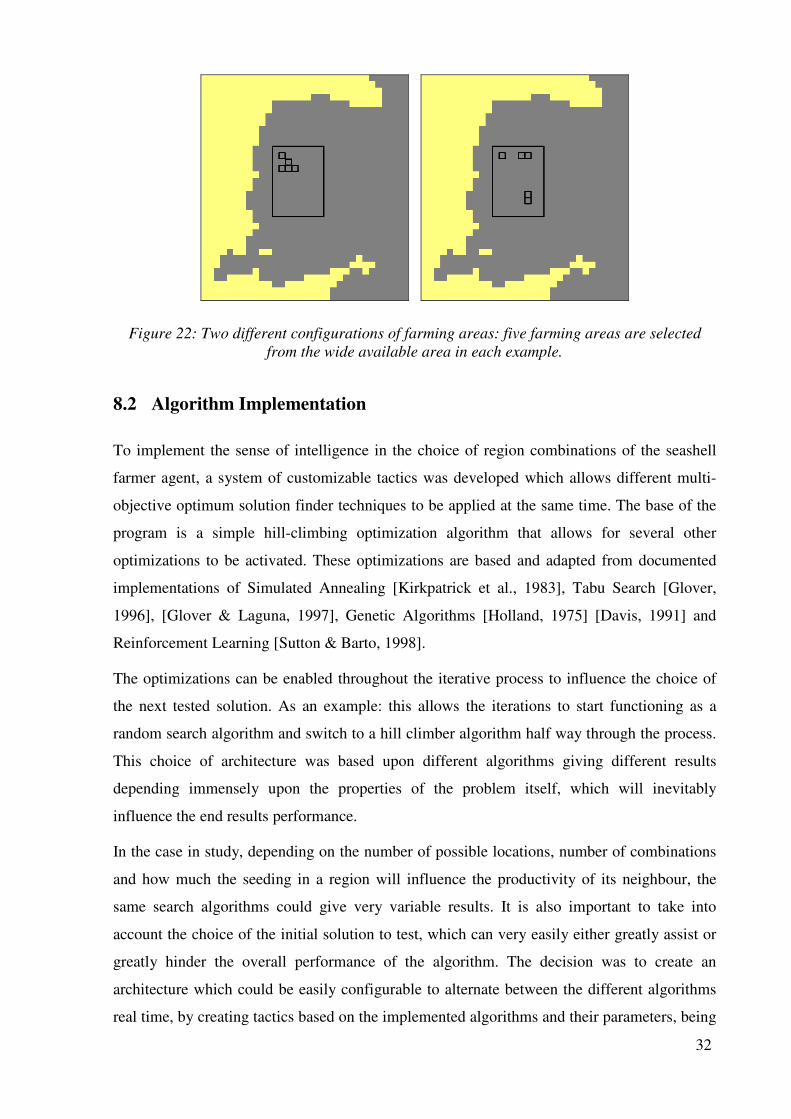
32

Figure 22: Two different configurations of farming areas: five farming areas are selected

from the wide available area in each example.

8.2 Algorithm Implementation

To implement the sense of intelligence in the choice of region combinations of the seashell

farmer agent, a system of customizable tactics was developed which allows different multi-

objective optimum solution finder techniques to be applied at the same time. The base of the

program is a simple hill-climbing optimization algorithm that allows for several other

optimizations to be activated. These optimizations are based and adapted from documented

implementations of Simulated Annealing [Kirkpatrick et al., 1983], Tabu Search [Glover,

1996], [Glover & Laguna, 1997], Genetic Algorithms [Holland, 1975] [Davis, 1991] and

Reinforcement Learning [Sutton & Barto, 1998].

The optimizations can be enabled throughout the iterative process to influence the choice of

the next tested solution. As an example: this allows the iterations to start functioning as a

random search algorithm and switch to a hill climber algorithm half way through the process.

This choice of architecture was based upon different algorithms giving different results

depending immensely upon the properties of the problem itself, which will inevitably

influence the end results performance.

In the case in study, depending on the number of possible locations, number of combinations

and how much the seeding in a region will influence the productivity of its neighbour, the

same search algorithms could give very variable results. It is also important to take into

account the choice of the initial solution to test, which can very easily either greatly assist or

greatly hinder the overall performance of the algorithm. The decision was to create an

architecture which could be easily configurable to alternate between the different algorithms

real time, by creating tactics based on the implemented algorithms and their parameters, being

33

customizable enough to allow proper fine tuning allowing for even better possible results. The

base algorithm is an adaptation of the common and heavily documented Simulated Annealing

with Monte Carlo probability.

The implemented Agents were [Cruz et al., 2007]:

• FarmerSA. The implemented Simulated Annealing (SA) algorithm follows the usual

guidelines of Kirkpatrick [Kirkpatrick et al., 1983], allowing the user to define some

common parameters like the initial temperature, final temperature and its rate of

descent. As documented amply over the literature, SA is based on a solution quality

evaluation threshold temperature formula, which increases the probability of choosing

the current test solution when it's better than the previous saved solution by passing

iteration of lowered temperature. The generic idea behind the algorithm is to allow the

system to explore enough of itself whilst the entropy of the search algorithm is high

enough to allow full (or plenty enough, at least) neighbour solution exploration and

then slowly start restricting it more and more, thus hopefully avoiding getting stuck in

local maximums instead of the global maximum (leading to the optimum solution). In

critic terms, it can work very well on some cases, but it can also take forever to find a

good solution only to fail in delivering the actual optimum. It depends on the

complexity/linearity of the solution search area itself, on how the neighbour solutions

are defined, on the speed of the temperature drop and on a hefty amount of luck with

the Monte Carlo probabilities. All in all, too many factors, which justify the decision

of not using exclusively this algorithm. A special parameter was added allowing the

algorithm to ignore the Monte Carlo probability comparisons if the user so desires to

always approve a new solution when it's quality is higher.

• FarmerTabu. The adaptation of Tabu Search [Glover, 1996], [Glover & Laguna,

1997], was called FarmerTabu and its implementation is based on maintaining a hash

list of all the previously tested solutions, so that when it is toggled on, it simply

prevents the simulation from choosing a previously tested solution as the next solution

to test, also keeping a counter of how many times the algorithm has taken to choose a

new and previously untested option from its choice of neighbours. The user can define

a threshold value for the counter of refused solutions to activate a special mutation

factor that serves to stir the process into other solution search paths after a certain path

has apparently overly explored without much success.

34

• FarmerGA. The FarmerGA implementation maintains a list of best solutions found so

far and crossbreeds them to form new combinations of regions. The user can define

the number of solutions to take into account as parents and the number of new breeds.

Unlike common Genetic Algorithms [Holland, 1975] [Davis, 1991], this FarmerGA

does not account for any mutation factor, which deems imperative that the list of

solutions used as parents contains combinations of regions as spread out through the

solution area as possible in order to achieve results that guarantee a solution not

restricted to a local maximum. The way the FarmerGA crossbreeds the parents list is

based on the quality hierarchy and one parameter configurable by the user. In crass

terms, it attempts to breed the best solution with all others in the tops list, the second

best with half of all the others, the third best with a third of all the others and so on.

The child genes are selected as the best individual locations amongst both parents, as

seen in Figure 23. The child is either listed to be tested or rejected depending on its

presence on the FarmerTabu list.

Figure 23: FarmerGA breeding result

• FarmerRL. The FarmerRL optimization is somewhat far from what is usually

referred to as Reinforcement Learning [Sutton & Barto, 1998]. This implementation

maintains a neighbours list for each possible region, containing information on its

neighbour locations quality for farming. As the test iterations occur, calculated

weights are summed to the quality of the areas selected in the tested solution,

increasing or decreasing its value. The value of the weight depends on the geometric

distance between the farming result of an individual zone and the average amongst all

the zones of the tested solution. The farming quality value of each region is taken into

account when the next selection of other neighbouring solutions for testing is

performed. So that, as more iterations occur the quality values of good seashell

farming regions gets higher and the quality values of bad seashell farming regions gets

lower, thus restraining the scope of search to the better regions. The strength of the

weight is configurable by the user and can vary in real-time. The definition of

neighbour solutions also influences greatly on how this optimization will perform.

There are 8 implemented types of choosing the next neighbour solution of FarmerRL:

15 – 0.345

16 – 0.346

24 – 0.332

25 – 0.339

34 – 0.341

9 – 0.345

11 – 0.341

24 – 0.342

27 – 0.341

33 – 0.347

9

15

16

24

33

35

1. Choosing the best neighbours of each position, using Monte Carlo probability factor.

2. Choosing the best neighbours of each position, only using Monte Carlo probability

factor for the positions below average quality.

3. Choosing the best neighbours of each position, without using Monte Carlo probability

factor.

4. Choosing the best neighbours of each position, without using Monte Carlo probability

factor, but changing only one of the positions.

5. Randomly shift all positions to their neighbours.

6. Randomly shift positions to their neighbours of only one of the positions.

7. Random search new position in positions below average quality.

8. All new positions completely randomly selected.

8.3 Tactics System

As previously mentioned a tactics system was developed to allow the users to configure the

real-time parameter reconfiguration of the implemented algorithms.

The base algorithm FarmerSA is always being applied and can be configured/parameterized

through a config.cfg text file. The parameters on this file will define the number of iterations

that the process will take to finish. This file also states which tactics file to use during the

process.

The other three remaining algorithms can be configured through the specific tactics file used.

This tactics file contains text lines which are referred to as toggles lines. These lines contain

the parameterization of the algorithms described previously. If these algorithms are not

toggled in this file to start at a given time frame of the process, they will not be used.

FarmerTabu and FarmerRL can be toggled on, re-parameterized or toggled off at any point in

time of the process. However, FarmerGA functions in a different manner as each toggle line

for FarmerGA will trigger the process of running the genetic crossing itself, it is expected to

only be toggled a few steps into the process so that it has time to build a large and wide spread

enough list of good results for its cross breeding.

Toggles for the same algorithm can be defined more then once per tactics file, typically

representing reconfigurations of the parameters at different time frames of the process. Each

line of the file contains several parameters: the algorithm it is configuring (Farmer SA,

FarmerTabu, FarmerGA, 2 for FarmerRL), the time frame in percentage during which it shall

be activated and the other values refer to the parameters of the specific algorithm.

36

8.4 Optimization Results

Several different tactics were tested on the Sungo Bay model to assist on determining the

optimum combination of 5 seashell farming regions out of the allowed seashell farming area.

Table 2 shows results of the best solution encountered by each of them after the fixed steps

iteration process was concluded for each different tactic.

Table 2: Results of the tactics tested

Tactic Result (Ton)

hillclimber 01 8019.14239 hillclimber 02 8027.93047

neigh 01 8051.82402

neigh 02 8053.85186 3GA 01 8049.96074 3GA 02 8050.86797

neighrand 01 8056.11995

neighrand 02 8055.06329 neighrand 03 8053.14825

totrand 01 8051.82402 totrand 02 8051.82402

Figure 24 shows the development throughout the iterations of tactic neighrand 01. As an

example, this tactic was scripted to have FarmerTabu on at all times, had 2 instances of

FarmerGA occurring once at half way through the simulation and again at 80%. Its FarmerRL

changed three times through the process to alter its neighbour selection parameters.

Testing the different tactics under the same conditions in short time period simulation

provided us with several different combinations of locations which can later be tested in long

time period simulations for validation of results.

7920

7940

7960

7980

8000

8020

8040

8060

8080

1 11 21 31 41 51 61 71 81 91 101 111 121 131 141 151 161 171 181 191 201 211 221 231 241 251 261 271 281 291 301 311 321 331 341

Iterations

We

igh

t

Figure 24: Neighrand 01 optimization results evolution

37

The best results from our tests can be seen in Table 3. Analyzing the test results we could

conclude that the best farming regions of the area are located on the lower bottom of our

global search area of 90 zones. There is a strong possibility that other, more optimum

combinations could be found by re-analyzing the problem concentrating on that area alone.

Table 3: Best solutions achieved

Location Weight (Ton)

81 1613.490035 82 1612.912944 83 1612.423538 72 1611.792726

80 1613.570428 Total weight 8056.11995

A reminder must be added that our program is based on a random initial search solution. The

fact that all of the tactics converged to similar solutions (containing a majority of elements in

early 80s locations) reassures us the quality of the location as a most profitable zone to

explore seashell farming.

38

9 Conclusions and Future Work

Considering the work plan of the ABSES project, the objectives programmed for the first

three years of the project were achieved. Several papers were published during the third year

concerning the models developed for our test sites, the calibration agent developed and the

aquaculture agents and their use to optimize bivalve production in aquaculture scenarios. A

PhD thesis and a MSc thesis are almost finished containing most of the project final results

and several papers are under evaluation for international journals and conferences containing

the project final results.

The execution of this project throws several important conclusions. The first conclusions are

related with the ecological modelling process and ecological simulator development:

• Ecological modelling is a complex process and model calibration is a very hard and

cumbersome task.

• EcoDynamo enables very realistic coastal ecological simulations including most of the

physical, chemical and biological processes of the ecosystem.

Some of the main conclusions are related with the benefits gained by using a multi-agent

simulator system:

• Separation of the visualisation into a different application enable to run the simulations

faster and to perform online and offline viewing of the simulation process whenever it

is desired.

• The use of an independent Calibration agent makes the system much more flexible.

Also, generic calibration agents may be constructed to be used in these type or other

types of simulations.

• New agents representing other entities that influence the ecological simulation may be

added in a very natural way. This process makes the simulation realism concerning the

human factor an incremental process. This enables the execution of simulations in

which humans are modelled by very simple rules but, progressively, introduce human

complex reasoning in the simulation process.

• The use of optimization and machine learning techniques may be a sound approach to

implement iterative procedures that may help to find optimal management scenarios.

Intelligent agents are a sound way to implement optimization and machine-learning

techniques both for calibration and optimization proposes.

39

Also, the development of a specific ecological simulation language brings several benefits:

• Complex simulation ecosystems are made much more comprehensible to the end

users. ECOLANG makes simulation experiments of complex ecosystems more

comprehensible to the humans and facilitates the interface with other applications.

• High-level messages facilitate the construction of agents that intermediate the

simulation and users by changing the system configuration between simulation

experiments or performing online supervision.

Regarding the use of optimization techniques for optimizing bivalve production the main

conclusion is that the management of coastal ecosystems may be performed in many different

ways and there is hardly one optimal solution, but most likely a “family” of “good”

management options. Giving the large complexity of these systems and the numerous

synergies between environmental conditions and management options, finding “good”

choices cannot be reduced to simple optimization algorithms, assuming linear or some defined

form of non-linear relationship between a set of parameters, variables and goal seeking

functions. Mathematical models may be very useful in finding “good” management solutions.

However, finding these may require many trial and error simulations and this is why using

agents that may look automatically for the mentioned solutions may be advantageous. This

requires the a priori definition of “good” solutions and constraints. For example, one may

wish to increase aquaculture production but keeping water quality within certain limits for

other uses. The approach followed for shellfish aquaculture optimization in coastal

ecosystems was based on the development of a seashell farming agent interacting with

EcoDynamo. The farmer agent optimizes seashell production by using known optimization

techniques for solving the problem of selecting the best farming regions’ combinations,

maximizing the productivity of the zone. This approach enabled to improve results achieved

by traditional approaches, improving the global profit achieved with bivalve production in the

ecosystem.

There is still plenty of research to be accomplished within the combined fields of ecological

simulation and multi-agent systems. There are many scenarios where intelligent programs

acting as agents could emulate and enhance the realistic behaviour of many different factors

within simulation systems. Decision support systems based on realistic ecological simulator

have much to gain with the inclusion of multi-agent systems interaction in their architecture

enabling its use for correct management of environmental resources towards sustainable

development.

40

References

[Barteneva et al., 2006] Daria Barteneva, Nuno Lau, Luis Paulo Reis, 2006. Implementation of

Emotional Behaviors in Multi-Agent System using Fuzzy Logic and Temperamental Decision

Mechanism, Proceedings of EUMAS 2006, Fourth European Workshop on Multi-Agent Systems,

Lisbon, Portugal.

[Barteneva et al., 2007] Daria Barteneva, Luis Paulo Reis & Nuno Lau, 2007. Bilayer Agent-Based

Model Of Social Behavior: How Temperament Influence On Team Performance, In: I. Zelinka, Z.

Oplatková and A. Orsoni (eds), Proceedings of the 21st European Conference on Modelling and

Simulation, pp. 181-187, Prague, Czech Republic. ISBN: 0-9553018-2-3 (978-0-9553018-2-7).

[Cruz et al., 2007] Filipe Cruz, António Pereira, Pedro Valente, Pedro Duarte & Luís Paulo Reis, 2007.

Intelligent Farmer Agent for Multi-Agent Ecological Simulations Optimization. In: J. Neves, M.

Santos and J. Machado (eds): EPIA 2007, LNAI 4874, pp.593-604. Springer-Verlag, Berlin

Heidelberg. ISBN: 978-3-540-77000-8 (978-3-540-77002-2_50)

[Cruz, 2006] Filipe Cruz, 2006. Desenvolvimento de Agente Aquicultor Inteligente, Relatório de

Estágio/Projecto de Fim de Curso em Engenharia Informática e Computaçao, Faculdade de

Engenharia da Universidade do Porto.

[Davis, 1991] L. Davis, 1991, Handbook of Genetic Algorithms, Van Nostrand Reinhold, NY

[Duarte et al., 2003] Pedro Duarte, R. Meneses, A. J. S. Hawkins, M. Zhu, J. Fang, & J. Grant, 2003.

Mathematical Modelling to Assess the Carrying Capacity for Multi-Species Culture Within

Coastal Water. Ecological Modelling, Vol. 168, pp. 109-143.

[Duarte et al., 2006a] Pedro Duarte, B. Azevedo, M. Guerreiro, C. Ribeiro, R. Bandeira, A. Pereira, M.

Falcão, D. Serpa, & J. Reia, Biogeochemical Modelling of Ria Formosa (South Portugal).

Hydrobiology

[Duarte et al., 2006b] Pedro Duarte, M. J. Guerreiro, J. Reia, L. Cancela da Fonseca, A. Pereira B.

Azevedo, M. Falcão, D. Serpa, C. Ribeiro & R. Bandeira, 2006. Ferramentas de Gestão de Zonas

Costeiras: Aplicação à Ria Formosa (Sul de Portugal). Proceedings do 2º Seminário sobre

Sistemas Lagunares Costeiros, Vila Nova de Santo André.

[Duarte et al., 2007a] Pedro Duarte, Maria J. Guerreiro, João Reia, Luis Cancela da Fonseca, António

Pereira, Bruno Azevedo, Manuela Falcão & Dalila Serpa, 2007. Gestão de zonas costeiras:

aplicação à Ria Formosa (Sul de Portugal). Revista Ciência Agronômica, v.38, n.1, pp.118-128.

ISSN 0045-6888.

41

[Duarte et al., 2007b] Pedro Duarte, Bruno Azevedo, C. Ribeiro, António Pereira, Manuela Falcão,

Dalila Serpa, Rui Bandeira & João Reia, 2007. Management Oriented Mathematical Modelling of

Ria Formosa (South Portugal). Transitional Water Monographs. 1:1. pp. 13-51.

[Falcão et al., 2003] M. Falcão, ,L. Fonseca, D. Serpa, D. Matias, S. Joaquim, P. Duarte, A. Pereira,, C.

Martins & M. J. Guerreiro, 2003. Synthesis report. EVK3-CT-20022-00084.

[Ferreira et al., 1998] J. Ferreira, P. Duarte, & B. Ball, 1998. Trophic Capacity of Carlingford Lough

for Aquaculture - Analysis by Ecological Modelling. Aquatic Ecology, Vol. 31 (4), pp. 361–379.

[Glover & Laguna, 1997] F. Glover, M. Laguna, 1997, Tabu Search, Kluwer Academic Publishing

[Glover, 1996] F. Glover, 1996, Tabu Search and Adaptive Memory Programming: Advances,

Applications and Challenges, Interfaces in Computer Science and Operational Research, Kluwer

Academic Publishing, pp. 1-75

[Guo et al., 1999] X. Guo, ,S. Ford & F. Zhang, 1999. Molluscan Aquaculture in China. Journal of

Shellfish Research, Vol. 18, pp. 19-32.

[Holland, 1975] J. H. Holland, 1975, Adaptation in Natural and Artificial Systems, University of

Michigan Press, AnnArbor

[Kirkpatrick et al., 1983] S. Kirkpatrick, C. D. Gelatt Jr & M. P. Vecchi, 1983, Optimization by

Simulated Annealing, Science, Vol. 220, No. 4598, pp. 671–680

[Naur, 1960] P. Naur, (ed.). 1960. Revised Report on the Algorithmic Language ALGOL 60,

Communications of the ACM, Vol. 3 No.5 (May), pp. 299-314.

[Norvig & Russel, 2003] P. Norvig & S.J. Russel. 2003. Artificial Intelligence: a Modern Approach,

2nd

edition, Prentice Hall.

[Osman, 1995] I. H. Osman, 1995. An introduction to Meta-Heuristics. In: Lawrence M, Wilsdon C

(eds). Operational Research Tutorial 1995. Operational Research Society: Birmingham, pp. 92-

122

[Pereira et al., 2004] António Pereira, Pedro Duarte & Luís Paulo Reis. 2004. Agent-Based Simulation

of Ecological Models. In: H. Coelho and B. Espinasse (eds), Proceedings of the 5th Workshop on

Agent-Based Simulation, pp. 135-140, Lisbon, Portugal, May. ISBN: 3-639150-31-1.

[Pereira et al., 2005a] António Pereira, Luis Paulo Reis & Pedro Duarte, 2005. ECOLANG - A

Communication Language for Simulations of Complex Ecological Systems. In Y. Merkuriev, R.

Zobel and E. Kerckhoffs (eds.) Proceedings of the 19th European Conference Modelling and

Simulation, ECMS’2005, pp. 493-500, Riga Latvia, 2005, ISBN: 1-84233-112-4

[Pereira et al., 2005b] António Pereira & Pedro Duarte, 2005 EcoDynamo – Ecological Dynamics

Model Application. University Fernando Pessoa – Centre for Modelling and Analysis of

Environmental Systems, Technical Report.

42

[Pereira et al., 2007] António Pereira, Pedro Duarte & Luís Paulo Reis, 2007. An Integrated Ecological

Modelling and Decision Support Methodology. In: I. Zelinka, Z. Oplatková and A. Orsoni (eds),

Proceedings of the 21st European Conference on Modelling and Simulation, pp.497-502, Prague,

Czech Republic. ISBN: 0-9553018-2-3 (978-0-9553018-2-7).

[Reis & Lau, 2002] Luís Paulo Reis & Nuno Lau, COACH UNILANG – A Standard Language for

Coaching a (Robo) Soccer Team, in Andreas Birk, Silvia Coradeschi and Satoshi Tadokoro,

editors, RoboCup-2001: Robot Soccer World Cup V, Springer Verlag Lecture Notes in Artificial

Intelligence, Vol. 2377, pp.183-192, Berlin, 2002

[Reis, 2003] Luís Paulo Reis, Coordenação em Sistemas Multi-Agente: Aplicações na Gestão

Universitária e Futebol Robótico, PhD Thesis/Tese de Doutoramento, Faculdade de Engenharia

da Universidade do Porto, June, 2003

[Restivo & Reis, 2006] André Restivo & Luis Paulo Reis, 2006. Clustering Agent Optimization

Results in Dynamic Scenarios, Proceedings of EUMAS 2006, Fourth European Workshop on

Multi-Agent Systems, Lisbon, Portugal.

[Restivo, 2006] André Restivo, 2006 . Dynamic Scenario Simulation Optimization, MSc Thesis,

Mestrado em Inteligência Artificial e Sistemas Inteligentes, Faculdade de Engenharia da

Universidade do Porto.

[Sutton & Barto, 1998] Richard Sutton & Andrew Barto, 1998, Reinforcement Learning: An

Introduction, MIT Press, Cambridge, MA, A Bradford Book

[Valente et al., 2008] Pedro Valente, António Pereira & Luís Paulo Reis, 2008, Calibration Agent for

Ecological Simulations: A Metaheuristic Approach, In: Oliveira, E., Sousa, A. (eds) Proceedings

of DSIE '08 — Doctoral Symposium on Informatics Engineering, FEUP Edições, Colecção

Colectâneas, pp. 64-75, February 7-8, Porto

[Vreugdenhil, 1989] C. B. Vreugdenhil, 1989. Computational Hydraulics, An Introduction. Springer-

Verlag, 183 pp.

[Weiss, 1999] G. Weiss, 1999. ed., Multi-Agent Systems: A Modern Approach to Distributed Artificial

Intelligence, MIT Press.

[Wooldridge, 2002] M. Wooldridge, 2002. An Introduction to Multi-Agent Systems, John Wiley &

Sons, Ltd.