Comprehensive Summaries of Uppsala Dissertationsfrom the Faculty of Science and Technology 622

_____________________________ _____________________________

Thin Films and Deposition Processes Studied by Soft X-Ray Spectroscopy

BY

BJÖRN GÅLNANDER

ACTA UNIVERSITATIS UPSALIENSISUPPSALA 2001

Dissertation for the Degree of Doctor of Philosophy in Solid State Physics presentedat Uppsala University in 2001

AbstractGålnander, B. 2001. Thin Films and Deposition Processes Studied by Soft X-RaySpectroscopy. Acta Universitatis Upsaliensis. Comprehensive Summaries of UppsalaDissertations from the Faculty of Science and Technology 622. 80 pp. Uppsala.ISBN 91-554-5006-7.

This thesis deals with studies of thin films using soft x-ray emission spectroscopy.Thin films are frequently used in optical, semiconductor and magnetic applications,and along with the development of thin film deposition techniques, there is a growingneed for thin film characterisation and production control. Soft x-ray spectroscopyprovides elemental as well as chemical bonding information and has the advantage ofbeing relatively insensitive to electric and magnetic fields. It may thus be used in-situduring deposition for monitoring sputtering deposition.

Thin films of TiVN were reactively co-sputtered using two targets, and soft x-ray spectroscopy and optical emission spectroscopy were used to determine the filmcomposition in-situ. These measurements were compared with ex-situ elementalanalysis as well as with computer simulations. The results agree qualitatively andindicate that soft x-ray spectroscopy can be used for in-situ determination of filmcomposition. In another study, the composition of chromium nitride was studied in-situ under varying deposition conditions. The fraction of different stoichiometricphases in the deposited films as a function of nitrogen flow was determined in-situ.

The thesis also deals with the angular dependence of soft x-ray emissionspectroscopy. The angular dependence of the emission was measured and comparedto simulations for layered samples consisting of different transition metals, onesample consisting of Fe(50Å)/Cu(100Å)/V(100Å)/Si and another set of samplesconsisting of Fe(XÅ)/V(100Å)/MgO, where X = 25, 50 and 100 Å. The measuredangular variation can be described qualitatively by calculations including refractiveeffects. For measurements below the critical angle of reflection, only the top layercorresponding to the evanescent wave region of 20–50 Å is probed, whereas forlarger grazing angles the probe depth reaches thousands of Å. This demonstrates thefeasibility of using the angular dependence as a way of studying composition andlayer thickness of thin films.

Björn Gålnander, Department of Materials Science, The Ångström Laboratory,Uppsala University, Box 534, SE-751 21 Uppsala , Sweden

© Björn Gålnander 2001

ISSN 1104-232XISBN 91-554-5006-7

Printed in Sweden by Lindbergs Grafiska HB, Uppsala 2001

"…But soft! what light through yonder windowbreaks?It is the east, and Juliet is the sun…"

ShakespeareRomeo and Juliet, Act II. Scene II

Papers included in the thesis

I Nyberg T., Skytt P., Gålnander B., Nender C., Nordgren J., Berg S.In situ diagnostic studies of reactive co-sputtering from two targets bymeans of soft x-ray and optical emission spectroscopyJ. Vac. Sci. Technol. A 15, 145-148 (1997).

II Nyberg T., Skytt P., Gålnander B., Nender C., Nordgren J., Berg S.Studies of reactive sputtering of multi-phase chromium nitrideJ. Vac. Sci. Technol. A 15, 248-252 (1997).

III Skytt P., Gålnander B., Nyberg T., Nordgren J., Isberg P.Probe depth variation in grazing exit soft-X-ray emission spectroscopy.Nucl. Instr. and Meth. in Phys. Res. A 384, 558-562 (1997).

IV Gålnander B., Käämbre T., Blomquist P., Nilsson E., Guo J., Rubensson J.-E., Nordgren J.Non-destructive chemical analysis of sandwich structures by means of softX-ray emission.Thin Solid Films 343-344, 35-38 (1999).

V Gålnander B., Saleem F, Tesfamichael T, Rubensson J. -E., Guo J. -H.,Butorin S. M., Såthe, C., Nordgren, J.Anodized aluminum oxide films studied by soft x-ray spectroscopy.In manuscript.

TABLE OF CONTENTS

1 Introduction 72 Theoretical considerations 10

2.1 Soft x-ray emission and absorption spectroscopy 102.2 Scattering and dispersion theory 11

2.2.1 Scattering cross sections 112.2.2 Dispersion and refractive index 16

2.3 Optical constants in the soft x-ray region 263 Experimental 29

3.1 Soft x-ray emission spectroscopy 293.1.1 Dispersion of radiation 293.1.2 Concave grating spectrometers 30

3.2 Radiation sources 343.2.1 Electron beam excitation 343.2.2 Synchrotron radiation sources 35

3.3 Soft x-ray absorption spectroscopy 373.4 Thin film deposition by reactive sputtering 39

3.4.1 General 393.4.2 Sputtering 403.4.3 Reactive sputtering 42

4 In-situ thin film analysis using soft x-ray spectroscopy 484.1 Two-target sputtering 484.2 Chromium nitride 51

5 Angular dependence of soft x-ray emission 545.1 Related grazing angle techniques 54

5.1.1 Grazing incidence techniques 545.1.2 Grazing exit techniques 565.1.3 X-ray emission studies using electron excitation 56

5.2 Grazing exit studies on layered samples 575.3 Discussion 615.4 Summary 67

6 Aluminium and nickel oxide films studied with soft x-ray spectroscopy 696.1 Anodised aluminium oxide 696.2 Nickel oxide for electrochromic applications 69

7 Concluding remarks 72References 74

1 INTRODUCTION

Thin films are used in many applications and for different purposes, such as glasscoatings, optically selective coatings and in magnetic and semiconductor structures.Single as well as multilayer thin films are important both for scientific and industrialpurposes.

There are a number of different techniques for producing thin films, with depositionconditions varying from ultra-high vacuum to atmospheric pressures. Along with thedevelopment of different deposition techniques there is an increasing demand forproduction control and characterisation of materials, both in-situ and ex-situ. There are anumber of different techniques for analysing thin films to obtain structural and chemicalinformation. Standard methods for analysing thin films, such as Auger electronspectroscopy and x-ray photoelectron spectroscopy, require ultra-high vacuum conditionsand can be difficult to use in-situ in a deposition environment. The electronspectroscopies are also sensitive to the high fields and charged particles associated with adeposition process such as sputtering and therefore cannot be used in-situ duringdeposition. Soft x-ray emission spectroscopy is another spectroscopic technique withincreasing usage both in fundamental and more applied research. It has the inherentadvantage of probing photons, which are not as sensitive to the environment as chargedparticles.

Process control is crucial in high-rate deposition of many compound materials in order tocontrol the composition. Another important issue is computer modelling of the sputteringprocess, which can be used to predict the behaviour of the reactive sputtering process. Inthis thesis the soft x-ray technique is used for analysing the growing thin film in-situ andfor comparison with modelling results. Soft x-ray spectroscopy probes photons fromelectronic transitions involving the valence band, and since the valence band isinfluenced by the neighbouring atoms this gives chemical sensitivity. This means that theemission from, for instance, a metal and a metal-oxide are different, something which isvery valuable when studying thin films. In this thesis, the chemical sensitivity is used forinstance in a study of reactively sputtered CrN, a material with different stoichiometricphases that can be distinguished in soft x-ray emission.

When analysing thin films it is in many cases important to have control over the probedepth of the analysis method. In soft x-ray emission spectroscopy this can be achieved byvarying the excitation parameters, such as the angle or energy of the electrons in case of

8

electron excitation. Another way is to change the angle of detection. When detecting theemitted photons in a small grazing angle from the sample, almost parallel to the samplesurface, only emission from a very thin surface layer of about one nanometer is detected.On the other hand, when detecting the radiation at larger grazing angles, or almostperpendicular to the sample surface, the technique becomes bulk sensitive, with emissiondetected from a depth of about one-hundred nanometers or more. This means that the softx-ray emission spectroscopy technique has a potential for depth profiling.

Historical notes

The technique used in this study, soft x-ray spectroscopy, saw its light in 1895 whenWilhelm Conrad Röntgen, then a professor in Würzburg, discovered the mysteriousx-rays.1 Almost immediately x-rays were used in medical imaging due to theirpenetrating nature. In 1905 Barkla demonstrated the polarisability of x-rays, implyingtheir transverse wave nature, and later also discovered the different K and L series of theradiation through absorption measurements. The big step towards x-ray spectroscopycame with the discovery by von Laue in 1912 and by Bragg, father and son, in 1913, thatx-rays could be diffracted in crystals. Bragg diffraction could be used to select thewavelength of x-rays and, taking advantage of this, Moseley found that the characteristiclines in the x-ray spectrum varied systematically with the atomic number of the element.The systematic study of x-ray emission and absorption spectra was continued and refinedby Manne Siegbahn and co-workers in Lund and later in Uppsala—Manne Siegbahnmoved to Uppsala in 1922 where he continued the work on x-rays until about 1935. Themeasurements were also extended to longer wavelengths, the soft x-ray region, by usinggratings instead of crystals to select the wavelength [3]. The systematic measurements ofMoseley and Siegbahn provided important experimental support for the development ofatomic theory by Bohr and Sommerfeld.

Soft x-ray spectroscopy was important also in the development of solid state physics. Inthe 1930s O'Bryan and Skinner [4,5] reported soft x-ray emission spectra of metals suchas beryllium and aluminium, showing a relatively broad band with a sharp cut offcorresponding to the Fermi edge, supporting the theory of metals developed bySommerfeld. Later Skinner also made studies of the temperature dependence of thebroadening of the edge, supporting the Fermi-Dirac theory [6].

Summary outline

This thesis summary is outlined as follows: This introductory chapter is followed inChapter 2 by a general background to the theory of soft x-ray spectroscopy and of theoptical properties in the soft x-ray region. In Chapter 3 some experimental details of softx-ray spectroscopy are presented, as well as a description of the reactive sputteringprocess. In Chapter 4, results from studies of thin films deposited by reactive sputteringare presented. In Chapter 5 an overview of different techniques using angular

1 For an historical introduction to x-rays see Refs. [1,2]

9

dependence of emission is presented along with results on layered samples studied usingsoft x-ray spectroscopy with varying exit angle. In Chapter 6, preliminary results frommeasurements on anodised, porous aluminium films and on sputtered nickel oxide filmsfor electrochromic applications are presented. In Chapter 7, some concluding remarks arepresented.

2 THEORETICAL CONSIDERATIONS

This chapter gives an introduction to the spectroscopic methods used in this thesis. Thetheoretical background to the soft x-ray emission and absorption processes are brieflydiscussed in section 2.1. A more thorough background to the optical properties and waysof measuring optical constants in the soft x-ray region is given in sections 2.2 and 2.3.

2.1 Soft x-ray emission and absorption spectroscopy

The transition probability for an emission process is given by quantum mechanicalperturbation theory and the result is often referred to as Fermi's Golden rule [7]. For(spontaneous) emission the transition probability within the dipole approximation can bewritten

Wfi (ω ) ∝ (hω )3 f er i2ρ f (Ei − hω) (2.1)

where er is the dipole operator. The initial state, i, corresponds to a core hole (coreionised or core-excited) state, and the final state, f, in a one-electron approximationcorresponds to a hole in the valence band. ρf, thus corresponds to the occupied density of

states in the valence band.2 The one-electron approximation means we see the transitionas involving only one electron, the electron which performs the transition from a valencelevel to the empty core-level. This approximation neglects the interaction between thecore-hole and the valence electrons and the dynamic interaction (correlation) between thevalence electrons as well as satellites due to multiple excitations [8]. This approximation,however, works well in the study of the band structure of solids [9].

From Eq. (2.1) we thus see that the transition probability is proportional to the occupieddensity of valence states if we neglect the ω3 dependence. However, the dipole matrixelement also gives us symmetry selectivity through the dipole selection rule, ∆l = ±1.Since the core-hole has a specific orbital symmetry, this means an initial core hole of s-symmetry will probe the p-density of states and an initial core-hole of p-symmetry willprobe the s-, and d-density of states.

2 Valence electrons here refers to the outermost occupied electron orbitals and we do not distinguishbetween conduction electrons in a metal or valence electrons in an insulator or semi-conductor.

11

If the valence orbitals are expanded into atomic-orbitals, or spherical harmonics, withspecific orbital quantum number, l,

ψ v = csϕs + cpϕp + cdϕd + ...

the dipole selection rule will probe the fraction of p-density of states, cp, for an s-corehole state and the cs and cd fractions for a p core-hole state. This is usually referred to as

the probing of partial density of states. This approach is well known for molecules,known as LCAO (linear combination of atomic orbitals) [10] but works also for solidswith quasi-free valence electrons, since a plane wave can be expanded in sphericalharmonics [7].This approach was already used in the early days [11] for explaining solid-state band spectra.

The symmetry selection of the dipole transitions together with the localised nature of thecore-hole means that the soft x-ray emission process probes the occupied local partialdensity of states, occupied LPDOS.

In x-ray absorption the transition probability is given by a similar expression as foremission Eq. (2.1), only the initial state corresponds to the ground state and the final statecorresponds to a vacancy in a core level and an electron added in an unoccupied valencestate. ρf in Eq. (2.1) then corresponds to the unoccupied density of states and XAS thus

probes the unoccupied LPDOS. If the incoming photon energy is large enough the core-electron can be ejected as a free electron (promoted to the continuum). This correspondsto x-ray photoemission.

2.2 Scattering and dispersion theory

2.2.1 Scattering cross sections

Scattering by an electron—scattering cross section

In scattering of light one assumes that the incoming light is a monochromatic,electromagnetic plane wave, with a specific phase dependence:

E(r ,t) = E0εei (k⋅r−ωt ) ,

where k is the wave vector of the incoming plane wave and ε is the polarisation vector.An electron can be accelerated by this incoming electric field and reradiate in a sphericalelectromagnetic wave. This process is thus generally referred to as scattering.

Consider a monochromatic linearly polarised electromagnetic plane wave incident on anelectron. From classical electromagnetism it can then be shown [12,13] that the scalar

12

electric field scattered by a free electron in a non-relativistic case is emitted in a dipolarmanner and can be written as

′ E (r,t) = −reEi

r(ε ⋅ ′ ε )ei( ′ k r−ω t ) (2.2)

where Ei is the incident electric field, ε and ε' are the polarisation vectors of the incoming

and scattered radiation respectively, and re =e2

4πε0mc2 is the classical electron radius3..

Figure 2.1. Illustration of the scattering process.

The scattering process is illustrated in Fig. 2.1. The polarisation dependence is given bythe factor ε ⋅ ′ ε in Eq. (2.2). If we consider the polarisation component in the scatteringplane (xz-plane), there is a cosϕ dependence in the scattered field. For the polarisation

component perpendicular to the scattering plane, i. e. in the y-direction, the polarisationfactor equals unity. Thus for unpolarised incoming radiation and if the polarisation of thescattered radiation is not measured we get an average contribution of

12 (1+ cos2 ϕ) from

the polarisation dependence to the scattered intensity .

The scattering cross section, σ, is defined as the ratio between scattered power and the

incoming power per unit area (intensity), σ = PscIi

, and is a measure of the scattering

efficiency of the incoming and scattered radiation is proportional to the absolute squared

field amplitudes, so that σ ∝ ′ E

2

E 2 . The differential cross section, dσdΩ

(θ ,φ ), is the fraction

of radiation intensity scattered into the solid angle dΩ(θ , φ) .

3 The classical electron radius is defined in the following way: The electrostatic energy of a sphere withradius R and charge e equal the rest mass of the electron, mc2 when R = re.

13

The differential scattering cross section for elastic scattering by a free electron, orThomson scattering, is then essentially given by squaring Eq. (2.2) and normalising with

the incoming intensity [12]

dσdΩ

= re2 ε ⋅ ′ ε 2 = re

2 12 (1+ cos2 ϕ) , (2.3)

where the last step is valid for the case of unpolarised incident radiation.

The total scattering cross section for a free electron, the Thomson cross section, is givenby integrating the differential scattering cross section, Eq. (2.3), over all solid angles

σ =8π3

re2 . (2.4)

It can be noted that the scattering Thomson cross section for a free electron, Eq. (2.4), isindependent of wavelength.4

Scattering from an atom—a collection of electrons

For an atom which is a collection of electrons bound to the nucleus with different bindingenergies, the elastic scattering becomes more complicated than for free electrons. In asimple classical model, an electron in an atom can be seen as a harmonic oscillator with aresonance frequency ωs corresponding to a certain binding energy. We also introduce adamping factor γ to account for dissipative losses such as radiation damping and othernon-radiative processes. The scattered electric field then has a specific frequencydependence, dispersion, and can be written [13]

′ E (r,t) = −

reEi(ε ⋅ ′ ε )r

ω 2

ω 2 − ωs2 + iγω

ei( ′ k r−ω t ) . (2.5)

The corresponding scattering cross section for a bound electron with resonantfrequency ω s is then

σ(ω) =8π3

re2 ω4

(ω 2 − ωs2 )2 + (γω)2 (2.6)

From the expression for the scattering factor for a bound electron, Eq. (2.6), we see thatfor low frequencies, ω <<ωs , the scattering can be approximated as

σ(ω) =8π3

re2 ω

ωs

4

=8π3

re2 λs

λ

4

(2.7)

4 There are limitations for higher energies where the photon momentum is high enough to cause recoil ofthe electron, resulting in inelastic, Compton, scattering.

14

which is the frequency dependence of Rayleigh scattering used by Lord Rayleigh toexplain the blue colour of the sky. Blue light with a wavelength of about 380 nm (3.3 eV)is scattered about 16 times as much in the atmosphere as red light with a wavelength ofabout 760 nm (1.6 eV). This explains both the blue appearance of the sky and the redcolour of the setting sun. The latter is an effect of blue light being preferentially scatteredaway during the propagation of the sunlight through the atmosphere. In the limit of highfrequencies, ω >>ωs , we see from Eq. (2.6) that the scattering cross section approaches

the Thomson scattering cross section and the bound electron scatters as if it were free.

If we consider elastic light scattering from an atom with more than one electron wegenerally also have to take the phase difference between scattering from differentelectrons into account. In this case the scattered electric field amplitude can be written

E(r,t) = −

reEi(ε ⋅ ′ ε )r

ω 2e−iQ⋅∆rs

ω 2 − ωs2 + iγωs=1

Z

∑

ei ( ′ k r −ω t ) (2.8)

The term in the bracket of Eq. (2.8) is the atomic scattering factor, which is a complexquantity defined as the ratio between the scattered electric field from an atom relative tothe scattered field from a free electron:

f (Q,ω ) =

ω 2e−iQ⋅∆rs

ω 2 − ωs2 + iγωs=1

Z

∑ . (2.9)

where Q ≡ ′ k − k is the momentum transfer, i. e. the difference between the incomingand scattered wave-vector and ∆rs is the position of the electron labelled s, relative to areference position which is most conveniently chosen at the nucleus. The scatteringfactor depends on the positions of the individual electrons through the phase factorQ ⋅ ∆rs which gives the scattering a certain angular dependence since

Q = 2k sin

ϕ2 =

4πλ

sinϕ2 (2.10)

where ϕ is the scattering angle, i. e. the angle between the incoming wavevector k andthe scattered wavevector k', see Fig. 2.2.

Figure 2.2. Illustration of momentum transfer in the scattering process.

15

If the wavelength, λ, is of the order of the size of the atom or less, the phase termsbecome significant since k = 2π

λ , but for longer wavelengths some simplifications are

possible as will be seen below. In general f (Q,ω) is a complex function and can be

written as

f (Q,ω) = f1 − if2 (2.11)

and the atomic scattering cross section can then be written

σat (ω ) =8π3

re2 f

2 =8π3

re2 f1

2 + f22( ) (2.12)

Looking closer at the phase term, Q ⋅ ∆rs , it can be estimated by

Q ⋅ ∆r ≤

4πλ

sinϕ2 ⋅ a (2.13)

where Q is given from Eq. (2.10) and ∆rs ≤ a where a is the dimension of the atom

which is of the order of the Bohr radius, a0 = 0.529 Å.

The case when Q ⋅ ∆rs << 1, and is called the forward scattering, or coherent scattering

region. The scattering factor f (Q,ω) then becomes independent on scattering angle

(momentum transfer) and can be written

f 0(ω ) =ω 2

ω2 −ωs2 + iγωs=1

Z

∑ (2.14)

where f 0(ω ) is called the forward scattering factor. From Eq. (2.13) we see that f 0(ω )can be used if ϕ << 1 and/or a λ <<1, that is for small scattering angles and/or

sufficiently long wavelengths (dipole approximation). For the soft x-ray and VUV regionwhere λ ranges from about 2 Å to 2000 Å, the forward scattering cross section can beused in most cases. For the very special case of high enough frequencies so that thedispersion in Eq. (2.14) can be neglected (ω <<ωs ), but still sufficiently long

wavelengths so that the forward scattering factor can be used, we see that f 0(ω ) → Z andthe total scattering cross section can be written

σat (ω ) =8π3

re2 f

2 →8π3

re2 Z2 . (2.15)

The square dependence of the number of electrons means that the electrons scattercoherently, i. e. the scattering from each of the electrons in the atom has a definite phaserelation with the other electrons so that amplitudes rather than intensities are added. Thisexplains the name coherent scattering.

16

The limit for the forward scattering region is, according to Eq. (2.13) above,approximately

4πa

λsin

ϕ2 ≈ 1 (2.16)

so that for scattering angles less than

ϕc ≈ 2arcsin

λ4πa

(2.17)

the forward scattering approximation is valid. (For small angles Eq. (2.17) gives

ϕc ≈

λ2πa

). In order to get a numeric estimation of this critical angle the Thomas-Fermi

approximation of the atomic radius can be used [7]; a ≈ 0.5Z −1 3 Å. From this we canestimate the critical scattering angle as

ϕc ≈

Z1 3

hω(keV), (2.18)

using the small angle approximation. For angles much larger than those given byEq. (2.17), the electrons in the atom will scatter incoherently, so that intensities are addedrather than amplitudes, giving an atomic scattering cross section proportional to Z insteadof Z2. This means that for shorter wavelengths the elastic scattering is strongly peaked inthe forward direction for atoms with many electrons.

2.2.2 Dispersion and refractive index

Dispersion—classical treatment

As shown in section 2.2.1 above, the forward scattering factor can be used in most casesin the soft x-ray region, and as we will see later, the forward scattering factor is directlyconnected with the index of refraction in the x-ray region. In the following we willtherefore consider only the forward scattering factor and concentrate on the frequencydispersion.

When discussing the dispersion it is customary to introduce the concept of oscillatorstrengths, gs, which in a simple semi-classical model correspond to the number ofelectrons with resonance frequency, ωs. The oscillator strengths in this simple model thustrivially obey the sum rule gs

s∑ = Z . The forward scattering factor, Eq. (2.14) can then

be written as

f 0(ω ) =gsω

2

ω 2 − ωs2 + iγωs

∑ (2.19)

17

As an adaptation to a more realistic behaviour as described from spectroscopicmeasurements, we have to introduce fractional oscillator strengths, gkn, having non-

integer values. As we shall see, these arise naturally as transition probabilities, or matrixelements, between different atomic states in a quantum mechanical treatment. Thesetransition probabilities correspond to transitions between different atomic energy states,or in a simple one-electron model we may say transition between different electronicenergy levels. The forward scattering then can be expressed as

f 0(ω ) =gknω 2

ω 2 − ω kn2 + iγωk≠n

∑ (2.20)

were ωkn corresponds to the energy difference between two atomic energy states;

hωkn

= En

− Ek. These fractional oscillator strengths obey a sum rule known as the

Thomas-Reiche-Kuhn sum rule [14,15]:

gknn=1

∞

∑ = Z . (2.21)

In our case we have assumed that the initial state is the ground state, k = 0, but the sumrule is valid also for excited initial states, k ≠ 0, allowing for the possibility of absorption.Again, we see from Eq. (2.20) and Eq. (2.21), that, f

0(ω ) → Z , when the frequency ismuch higher than the resonance frequencies.

Dispersion-quantum mechanical description

For a quantum mechanical description, the scattering amplitude in a non-relativistic caseis given by the Kramers-Heisenberg formula, which was first derived from thecorrespondence principle [16]. If we use modern quantum mechanics the derivation ismost easily carried out using perturbation theory, with the incoming radiation field as aperturbation to the atomic system.

Consider the non-relativistic Hamiltonian for the unperturbed atomic electron:

H0 =p2

2m+ V (r). (2.22)

The electromagnetic field perturbation is introduced via the standard prescription [17]

p → p − qA = p + eA

18

where A is the electromagnetic vector potential5. The total Hamiltonian for the chargedparticle interacting with the electromagnetic field is then

H = H0 + Hint =1

2m(p + eA)2 + V(r) = (2.23)

1

2m(p2 + ep ⋅ A + eA ⋅ p + e2A ⋅ A) + V(r)

and the interaction Hamiltonian can thus be identified with

Hint =1

2m(ep ⋅ A + eA ⋅ p + e2A ⋅ A) . (2.24)

If we use the Coulomb gauge, ∇⋅ A = 0, which allows only transverse waves, Eq. (2.24)can be rewritten as6

Hint =1

2m(2eA ⋅p + e2A ⋅ A) . (2.25)

According to time-dependent perturbation theory for a harmonic perturbation, thetransition rate from the initial state, i , to the final state, f , is given by the so-called

Fermi golden rule [7,17]

Wf ←i =

2πh

M f i2δ (E f − Ei − h( ′ ω −ω )) (2.26)

where Et and Ei are the energy values of the final and initial atomic states respectively, ωis the frequency of the incoming photon and ω' the frequency of the outgoing, scatteredphoton. In the transition amplitude matrix element, Mfi , contributions from first and

second order perturbations are treated, M fi = M fi1 + M fi

2 + ... . In first order perturbation

only the A·A term in the interaction Hamiltonian, Eq. (2.25), contributes and the firstorder transition amplitude can be written

M fi(1) =

e2

2mf A ⋅ A i (2.27)

In second order perturbation the p·A term contributes, giving

M fi

(2) = −e2

m2f A ⋅ p n n A ⋅ p i

En − Ei + hωn∑ +

f A ⋅p n n A ⋅ p i

En − Ei + h ′ ω (2.28)

5 The electric and magnetic fields are related to A by E = −∇φ −

∂A∂t

; B = ∇ ×A6 If ∇⋅ A = 0 , then ∇⋅ Aψ = (∇ ⋅A)ψ + (A ⋅∇ )ψ = (A ⋅ ∇)ψ .

19

In these equations i , f and n represent the initial, final and intermediate states

respectively.

In general, the matrix elements in Eq. (2.27) and Eq. (2.28) should be evaluated using thequantised field version of the vector potential, A, which is then a quantum mechanicaloperator [17] The state vectors i , f and n then also should be interpreted as

including both the photon state and the atomic state, e. g. i = k ,ε( photon) ψ i(atom) ,

where the incoming photon is characterised by the wavevector k and the polarisationvector ε. The matrix elements can then be evaluated using the second quantisationformalism. It can be shown [17], however, that it is possible to use the followingequivalent classical vector potentials:

A = A0εeik⋅r− iω t = cN kh2ωV εeik⋅r−iω t

for absorption and

A = ′ A 0 ′ ε ei ′ k ⋅r− i ′ ω t = c(Nk +1)h

2 ′ ω V ′ ε e− i ′ k ⋅r+ i ′ ω t

for scattering or emission, where V is the quantisation volume, and Nk the photonoccupation number. In the following i , f and n represent only the atomic state

vectors. If we use these expressions the transition amplitudes, Eq. (2.27) and Eq. (2.28),can be evaluated giving [17,18]

M fi

(1) = ′ A 0A0ε ⋅ ′ ε f e i(k− ′ k )r i δ fi (2.29)

and

M fi

(2 ) = −e2

m2 ′ A 0A0f e−i ′ k ⋅r ′ ε ⋅ p n n e ik⋅rε ⋅ p i

En − Ei − hω+

f e ik⋅rε ⋅ p n n e−i ′ k ⋅r ′ ε ⋅ p i

En − Ei + h ′ ω

n∑

(2.30)

where k', and ω' corresponds to scattered photons and k, ω to incoming (absorbedphotons), compare Fig. 2.1. The first term in Eq. (2.30) is called the resonant term andcorresponds to the normal time ordering with absorption first and emission later. Thesecond term is non-resonant and corresponds to emission before absorption. This can beseen in the light of Heisenberg's uncertainty relation, ∆E ⋅ ∆t ≥ h 2, which allows such a

reversed time-ordering. For most practical cases, however, the second non-resonant termcan be neglected compared to the resonant term since the denominator is much larger forthe non-resonant term.

In the soft x-ray region it is customary to use the dipole approximation, i. e. to keep onlythe first, constant, term in the expansion e

ik⋅r ≅1 + ik ⋅r + (ik ⋅ r)2 2 +K. This is justified

20

as long as the wavelength is (much) larger than the atomic size, so that kr <<1. If we use

this approximation, Eqs. (2.29) and (2.30) above can be rewritten as

M fi

(1) = ′ A 0A0ε ⋅ ′ ε f i δ fi = ′ A 0A0 ε ⋅ ′ ε δ fi (2.31)

M fi

(2 ) = −e2

m2 ′ A 0A0f ′ ε ⋅ p n n ε ⋅ p i

En − Ei − hω+

f ε ⋅ p n n ′ ε ⋅p i

En − Ei + h ′ ω

n∑ (2.32)

If we consider a measurement of the scattering cross section in a solid angle dΩ, andfrequency range ω , ω + dω , we have to consider the density of photon states, or

radiation density, for the scattered photons. For a scattered photon in the range k, k+dk,the density of states is dNk = V

8π3 k2dkdΩ, where V is the quantisation volume, which in

terms of energy density can be written as dNh ′ ω = V

8π 3 c3′ ω 2

h d(h ′ ω )dΩ = ρhω d(h ′ ω )dΩ .

If this is used in the Golden rule expression, Eq. (2.26) and integration over scatteredphoton energy is performed, we obtain

dW fi

dΩdΩ =

2πh

M f i2δ (Ef − Ei − h( ′ ω −ω ))ρh ′ ω d(h ′ ω )dΩ

′ ω ∫

=

2πh

M f i2

ρh ′ ω dΩh ′ ω =hω −(E f −Ei )(2.33)

for the transition probability (photon/s) into a solid angle dΩ. In this integration we haveassumed that Ef and Ei are "sharp" non-degenerate stationary states, and that the

incoming photon beam is monochromatic. For continuum states or for extended,degenerate states in a solid we should also consider the electronic density of states in theintegration. Furthermore, if the final state, f, is an excited state with finite lifetime, weshould also take into account the lifetime broadening of the final state, Γf.

Writing out the transition matrix element, Mfi, we find that the differential scattering

cross section within the dipole approximation is

dσdΩ

= re2 ′ ω

ω

′ ε ⋅ εδ fi −

1

m

f ′ ε ⋅ p n n ε ⋅ p i

En − Ei − hω + iΓn+

f ε ⋅ p n n ′ ε ⋅p i

En − Ei + h ′ ω

n∑

f∑

2

h ′ ω =hω −(E f −Ei )

(2.34)

Equation (2.34) is the modified Kramers-Heisenberg equation since we have introduced alife-time broadening, Γn, for the intermediate state in the resonant term. This expression

is given for the case of a one-electron atom. Since the cross section is defined as the ratiobetween the scattered and incoming radiation intensities we have normalised to the

21

incoming intensity in Eq. (2.34). This is reflected in the factor ′ ω ω which is the ratio

between the scattered and incoming photon energies.

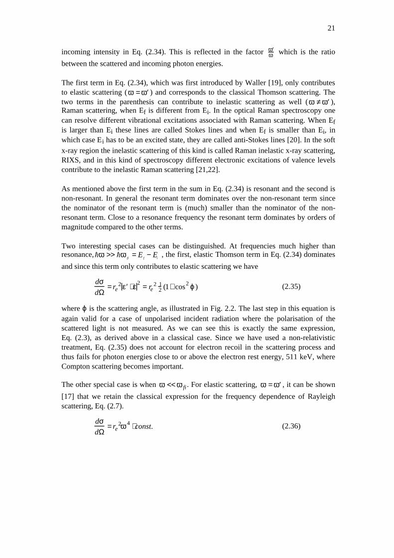
The first term in Eq. (2.34), which was first introduced by Waller [19], only contributesto elastic scattering (ω = ′ ω ) and corresponds to the classical Thomson scattering. Thetwo terms in the parenthesis can contribute to inelastic scattering as well (ω ≠ ′ ω ),Raman scattering, when Ef is different from Ei. In the optical Raman spectroscopy onecan resolve different vibrational excitations associated with Raman scattering. When Efis larger than Ei these lines are called Stokes lines and when Ef is smaller than Ei, inwhich case Ei has to be an excited state, they are called anti-Stokes lines [20]. In the soft

x-ray region the inelastic scattering of this kind is called Raman inelastic x-ray scattering,RIXS, and in this kind of spectroscopy different electronic excitations of valence levelscontribute to the inelastic Raman scattering [21,22].

As mentioned above the first term in the sum in Eq. (2.34) is resonant and the second isnon-resonant. In general the resonant term dominates over the non-resonant term sincethe nominator of the resonant term is (much) smaller than the nominator of the non-resonant term. Close to a resonance frequency the resonant term dominates by orders ofmagnitude compared to the other terms.

Two interesting special cases can be distinguished. At frequencies much higher thanresonance, hω >> hω

fi= E

f− E

i , the first, elastic Thomson term in Eq. (2.34) dominates

and since this term only contributes to elastic scattering we have

dσdΩ

= re2 ′ ε ⋅ ε 2 = re

2 12 (1+ cos2 ϕ) (2.35)

where ϕ is the scattering angle, as illustrated in Fig. 2.2. The last step in this equation isagain valid for a case of unpolarised incident radiation where the polarisation of thescattered light is not measured. As we can see this is exactly the same expression,Eq. (2.3), as derived above in a classical case. Since we have used a non-relativistictreatment, Eq. (2.35) does not account for electron recoil in the scattering process andthus fails for photon energies close to or above the electron rest energy, 511 keV, whereCompton scattering becomes important.

The other special case is when ω << ω fi . For elastic scattering, ω = ′ ω , it can be shown

[17] that we retain the classical expression for the frequency dependence of Rayleighscattering, Eq. (2.7).

dσdΩ

= re2ω 4 ⋅ const. (2.36)

22

Relation between forward scattering factor and refractive index

We now return to the forward scattering factor mentioned above. The importance of theforward scattering factor can be seen from its relation to the optical refraction index,n(ω). The relation between the forward scattering factor is seen by the fact that in ahomogeneous material, the scattered spherical waves recombine to form a secondaryplane wave in the forward direction. In all other scattering directions the scattered wavescancel in a homogeneous material.7 The secondary wave lags in phase 90˚ compared tothe incoming, primary, wave [23]. The secondary and primary waves will interfere andthe resultant wave is the refracted wave with the phase velocity c/n. This was shownrigorously at the beginning of the last century by Ewald [24] and Oseen [25] and is calledthe Ewald-Oseen extinction theorem [26].

The use of macroscopic material constants, such as the index of refraction, when theperturbing field has a wavelength close to the size of the scatterers is not entirelyobvious. In the soft x-ray region where the dipole approximation is still valid (λ > 1Å)this is acceptable, but for harder x-rays with λ < 1Å it is less obvious. The validity of theEwald-Oseen extinction theorem also for harder x-rays has been shown [27] using thefact that the electrons respond as free electrons for frequencies much higher than theircharacteristic frequency. This is the basis for using macroscopic indexes of refractionalso for shorter wavelengths.

The relation between the forward atomic scattering factor, f0(ω ), and refractive index,

n, can be shown by considering transmission through a slab of finite thickness consistingof atoms with a certain forward scattering factor f

0(ω ).The derivation was done byDarwin in 1914 [28] and is recapitulated in books by James [29] and Compton [14] andalso more recently by Henke et al [30]. A formally similar derivation for scattering bymacroscopic particles in the optical region is found in books on light scattering [31,32].8

The derivation will not be given in detail here, and the reader is referred to the referencesgiven above for more details. The scattered amplitude from a slab of thickness l which isthin compared to the scattering cross section so that multiple scattering can be neglected,is considered. (In the original treatment of Darwin one atomic plane in a crystal wasconsidered). The scattered radiation amplitude is considered at a distance z in thedirection of propagation, where it is assumed that z >> λ. If the scattered amplitude fromall the atoms, with scattering factor f

0(ω ), in the slab are added with its phase, it can beshown that the resulting amplitude corresponds to the contribution of scattered light fromhalf the first Fresnel zone, since adjacent Fresnel zones have different sign and thereforealmost cancel each other [23]. (The slab is considered infinite in the x and y directionsand uniformly illuminated). There is a resulting phase shift of –π/2 and the relation

7 Except for the case of Bragg scattering in crystals where scattered waves can interfere constructively inother directions as well.8 Note that in the literature of particle scattering the scattering factor is usually written S, and is related tothe atomic scattering factor by the relation S(0) = ikf (0) , for the forward scattering amplitudes [31,32].

23

between the amplitude, Esc, of the scattered wave and the amplitude, Ein, of the incoming

wave can be shown to be

Esc = Einλ Nat l f0(ω)ree−i π

2 = −iEinq (2.37)

where Nat is the atomic volume density. If we add the amplitudes of the scattered and the

incoming waves we get the amplitude of the resulting wave as

Etot = Ein + Esc = (1− iq)Ein ≈ Eine− iq .

The introduction of the slab of thickness l thus can be interpreted as having produced aphase change

∆φ = −q = −λNat l f 0(ω)re . (2.38)

This expression can be compared to the phase shift that we would get from consideringthe phase retardation due to a slab of thickness l with the macroscopical index ofrefraction n

∆φ = kln − kl = kl(n −1), (2.39)

i. e., the phase difference between a wave propagating a distance l through a medium ofrefractive index n, and a wave propagating a distance l through vacuum.

If we compare the expressions (2.38) and (2.39) we have

kl(n − 1) = −Natlλre f 0(ω)

so that

n1 + in2 =1− δ + iβ = 1−

λ2Natre

2π( f1

0 (ω) − if20(ω))

and

δ = λ2Natre

2πf1

0 (ω)

β = λ2Natre

2πf2

0 (ω)

(2.40)

which is the relation we obtain between the optical constants and the forward scatteringfactors.

24

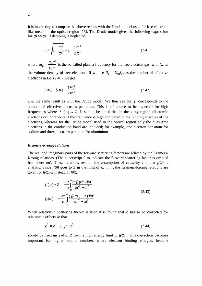
It is interesting to compare the above results with the Drude model used for free electron-like metals in the optical region [15]. The Drude model gives the following expressionfor ω >> ωp if damping is neglected:

n = 1 −ω p

2

ω2 ≈1 −1

2

ω p2

ω 2 (2.41)

where ω p2 =

Nee2

ε0m is the so-called plasma frequency for the free electron gas, with Ne as

the volume density of free electrons. If we use Ne = Natf1 , as the number of effective

electrons in Eq. (2.40), we get

n = 1− δ = 1−1

2

ω p2

ω 2 (2.42)

i. e. the same result as with the Drude model. We thus see that f1 corresponds to the

number of effective electrons per atom. This is of course to be expected for highfrequencies where f

0(ω ) → Z . It should be noted that in the x-ray region all atomicelectrons can contribute if the frequency is high compared to the binding energies of theelectrons, whereas for the Drude model used in the optical region only the quasi-freeelectrons in the conduction band are included; for example, one electron per atom forsodium and three electrons per atom for aluminium.

Kramers-Kronig relations

The real and imaginary parts of the forward scattering factors are related by the Kramers-Kronig relations. (The superscript 0 to indicate the forward scattering factor is omittedfrom here on). These relations rest on the assumption of causality and that f(ω) isanalytic. Since f(ω) goes to Z in the limit of ω → ∞ , the Kramers-Kronig relations aregiven for f(ω)–Z instead of f(ω):

f1(ω ) − Z = −2

π′ ω f2 ( ′ ω )d ′ ω

′ ω 2 − ω20

∞

∫

f2(ω) = −2ωπ

( f1( ′ ω ) − Z)d ′ ω ′ ω 2 − ω2

0

∞

∫(2.43)

When relativistic scattering theory is used it is found that Z has to be corrected forrelativistic effects so that

Z∗ = Z − Etot / mc2 (2.44)

should be used instead of Z for the high energy limit of f(ω) . This correction becomesimportant for higher atomic numbers where electron binding energies become

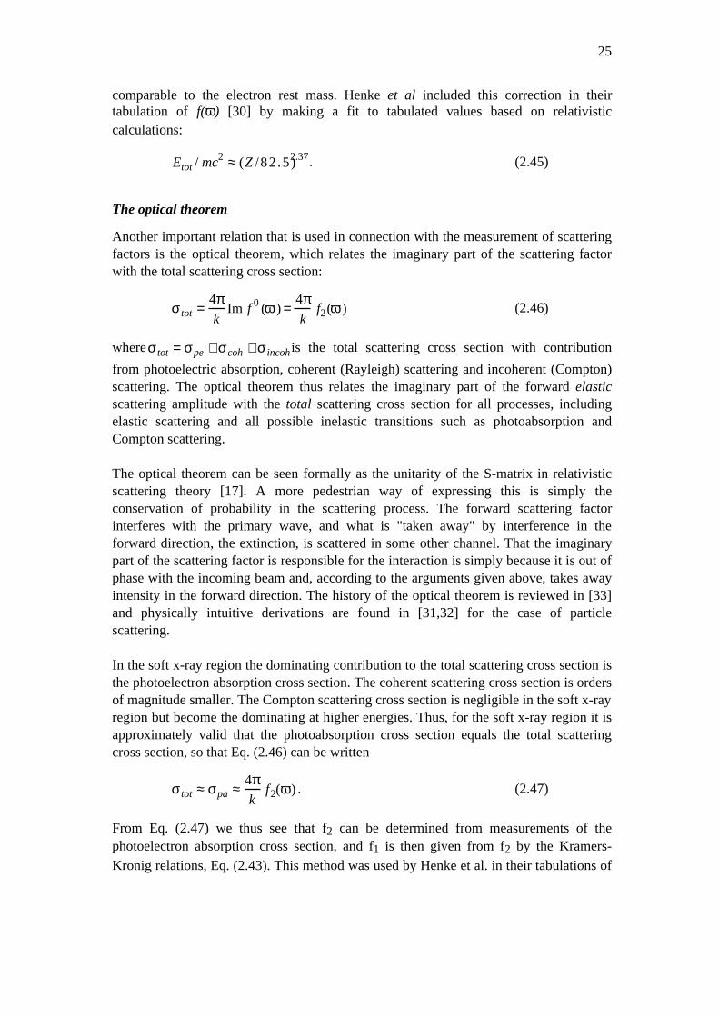
25

comparable to the electron rest mass. Henke et al included this correction in theirtabulation of f(ω) [30] by making a fit to tabulated values based on relativisticcalculations:

Etot / mc2 ≈ (Z /82 .5)2.37. (2.45)

The optical theorem

Another important relation that is used in connection with the measurement of scatteringfactors is the optical theorem, which relates the imaginary part of the scattering factorwith the total scattering cross section:

σ tot =

4πk

Im f 0 (ω ) =4πk

f2(ω ) (2.46)

whereσ tot = σpe + σcoh + σ incohis the total scattering cross section with contribution

from photoelectric absorption, coherent (Rayleigh) scattering and incoherent (Compton)scattering. The optical theorem thus relates the imaginary part of the forward elasticscattering amplitude with the total scattering cross section for all processes, includingelastic scattering and all possible inelastic transitions such as photoabsorption andCompton scattering.

The optical theorem can be seen formally as the unitarity of the S-matrix in relativisticscattering theory [17]. A more pedestrian way of expressing this is simply theconservation of probability in the scattering process. The forward scattering factorinterferes with the primary wave, and what is "taken away" by interference in theforward direction, the extinction, is scattered in some other channel. That the imaginarypart of the scattering factor is responsible for the interaction is simply because it is out ofphase with the incoming beam and, according to the arguments given above, takes awayintensity in the forward direction. The history of the optical theorem is reviewed in [33]and physically intuitive derivations are found in [31,32] for the case of particlescattering.

In the soft x-ray region the dominating contribution to the total scattering cross section isthe photoelectron absorption cross section. The coherent scattering cross section is ordersof magnitude smaller. The Compton scattering cross section is negligible in the soft x-rayregion but become the dominating at higher energies. Thus, for the soft x-ray region it isapproximately valid that the photoabsorption cross section equals the total scatteringcross section, so that Eq. (2.46) can be written

σ tot ≈ σpa ≈

4πk

f2(ω) . (2.47)

From Eq. (2.47) we thus see that f2 can be determined from measurements of thephotoelectron absorption cross section, and f1 is then given from f2 by the Kramers-

Kronig relations, Eq. (2.43). This method was used by Henke et al. in their tabulations of

26

scattering factors [30], where they used the average of available photoabsorption crosssection data together with calculated data for some energy regions.

2.3 Optical constants in the soft x-ray region

As already mentioned, the real part of the index of refraction in the soft x-ray region isusually less than unity and can be written n = 1–δ, where δ > 0 in general. We thus canexpect total reflection below a certain critical angle, θc ≈ 2δ . This is, however notstrictly valid close to the absorption edges where the coherent scattering factor, f(ω),decreases and occasionally becomes less than zero so that δ <0 and 1–δ >1, so that onecan expect "normal optical behaviour" there. Typical examples are the Si K and C K-edges [34,35].

Early measurements of the index of refraction in the x-ray region.

Already Röntgen tried to detect refraction of x-rays in solids. He used prisms of e. g.glass and aluminum, but did not discover anything since he was looking for a refractiveindex of the same order as in the optical region [14]. Stenström made measurements ofthe deviations from Bragg's law of x-ray diffraction in 1919. These deviations indicatedthe existence of a refractive index for x-rays and were in such a direction that the indexof refraction should be less than one. The measurements were performed on crystals ofgypsum and sugar in Siegbahn's laboratory in Lund [3]. These results led Compton to theinvestigation of total reflection at small glancing angles, which should follow by anindex of refraction less than one. Compton made measurements on crown glass andsilver "mirrors" using W L-emission of λ = 1.3 Å. The measurements confirmed totalreflection below a certain critical angle and from the relation θc ≈ 2δ he gave values ofδ of the order of 10–6 which is in agreement with a simple Drude-Lorentz theory [36].

In 1924 Larsson, Siegbahn and Waller [37] made measurements of the refraction of x-rays in a glass prism. Waller, who worked with the theory of the dispersion and influenceof heat motion on x-ray diffraction, suggested this type of measurement [37,38]. Theresults were in agreement with dispersion theory and gave δ = const ⋅ λ2 since themeasurements were carried out with wavelengths far away from any absorption edges ofthe atoms in the glass prism. This was a direct confirmation of the refraction of x-rays.Larsson later made more precise measurements of the refraction in a prism of quartzwhich were presented in his thesis [39]. The measurements were carried out at severaldifferent wavelengths, corresponding to the characteristic radiation of different targets ofthe x-ray tube, centred around the K-absorption edge of Si at 6.7 Å (1.8 keV). This wasin order to investigate the effects on the refractive index close to an absorption edge. Themeasurements were performed with great care and the results confirmed the "anomalous"dispersion effect close to the absorption edge, i. e. that δ deviates from the δ = const ⋅ λ2

behaviour expected from a free electron gas. It can be mentioned that the prism methodhas also been used more recently, for instance for the determination of dispersion inGaAs [40].

27

Modern methods used to determine optical constants

Measurements of optical constants/scattering factors are important, for instance, forpredicting the behaviour of optical elements such as mirrors in the soft x-ray region.Some measurement methods are mentioned here, and the reader is referred to othersources for more information: general overviews of optical constants are found forinstance in [41-43]. Different ways of measuring f1 in the x-ray region are reviewed in

[44]. The subject of x-ray dispersion corrections in general, calculations as well asmeasurements, for instance, are treated in [45,46].

The most common methods to determine optical constants, δ and β, and the relatedscattering factors, f1 and f2 , see Eq. (2.40), in the soft x-ray region are the following:

a) Transmission measurements to determine photoabsorption coefficients, (β)b) Measurements of reflection vs. angle and/or energy (δ, β).c) Interferometric methods to determine phase shift (δ).

There are other methods which can briefly be mentioned: in the lower energy region(VUV), ellipsometry can be used for the determination of δ and β up to ≈ 35 eV [47], andEELS can be used up to about 30 eV [48]. Angular dependent measurements ofphotoemission have also been used for the determination of optical constants [49,50].

a) Transmission measurements can be used to measure β and Kramers-Kronig transformsapplied to obtain the real part, δ. Transmission measurements for attenuation coefficientsin the x-ray region in general are reviewed in Ref. [51] and tabulations of attenuationcoefficients for different energies can, for instance, be found in Ref. [30,52,53]. In theEUV and soft x-ray region the absorption is relatively high and there is an experimentalproblem in producing sufficiently thin, free standing films for transmissionmeasurements. The films should be pin-hole free and homogeneous and of well-knownthickness. Measurements using carbon/metal multilayer films have been reported [54].The method of using co-evaporated carbon films for support and oxidation protection hasalso been used [55,56]. As an example, transmission measurement using free-standingfilms of C/Mo/C of different thickness for determination of the absorption coefficient ofMo in the energy range 60–930 eV was recently reported [55]. The thickness of the Molayer of different films varied between 300–1900 Å and the C layers were 145 Å thick.The authors used Kramers-Kronig analysis for the determination of δ and sum-rules tocheck for consistency.

b) Measurements of specular reflectivity vs. angle and/or energy at grazing angles aroundthe total reflection region can be used for the determination of δ and β [57]. The criticalangle in the case of small absorption can be used directly to determine δ through therelation θc ≈ 2δ . By fitting the reflectivity measurements to Fresnel calculations both δand β can be determined. Reflectance measurements suffer from the problem ofcontamination and surface roughness. Usually the surface roughness has to be known and

28

a contamination layer included in the evaluation of δ and β. The advantages are thatreflectance measurements can be used for determination of both δ and β and thatmeasurements can be performed on bulk samples which are applicable in cases wheresufficiently thin free standing films are hard to manufacture. As an example, opticalconstants of Si were recently determined by reflectivity measurements in the region50 eV–180 eV, since stress-free Si films for transmission measurements are hard tofabricate, and for the reason that highly polished and clean Si surfaces can be obtainedrelatively easily [58].

c) Interferometric methods are used mainly for harder x-rays (> 3 keV) since absorptionis lower here [44], but have also been applied in the soft x-ray region [59,60]. The firstmeasurements using interferometry were performed by Bonse and Hart [61]. Aninterferometer measures the phase shift by the propagation through a slab of a material,which can be used directly for the determination of δ.

In the comprehensive tabulation of f1 and f2 by Henke et al. [30], covering the energy

range 50 eV–30 keV, the authors used a compilation of available experimentalphotoabsorption data, together with theoretical calculations where experimental data issparse, in order to produce values for the best fit between different sources. In thesetabulations, f2 is given directly from photoabsorption data, Eq. (2.47) above, and f1 from

the Kramers-Kronig relations, Eq. (2.43). Updated versions of these tables are availableon-line [62]. Data from the Henke-tables were used in this thesis to calculate the angulardependence of soft x-ray emission, Chapter 5.

It should be noted, though, that the Henke-tables represent data of atomic scatteringfactors in the independent atomic approximation, i. e. that the atoms interact withradiation as if they were isolated atoms. This approximation is not valid close toabsorption edges where the local environment of the atom gives rise to a fine structure[63] in the absorption edge. The independent atom approximation also breaks down forlow energies (generally below 50 eV) where the band structure may influence the opticalbehaviour of materials.

3 EXPERIMENTAL

This chapter gives the experimental details of soft x-ray spectroscopy as applied to themeasurement in the thesis. It also treats the sputtering technique for thin film production.

3.1 Soft x-ray emission spectroscopy

Air at atmospheric pressure shows high absorption of electromagnetic radiation in thewavelength range 2000 Å to 2 Å, corresponding roughly to the energy range 6 eV to6 keV. A spectrometer in this region must therefore operate under vacuum. The range 50eV to 6 keV is called the soft x-ray region, SX, as opposed to the hard (penetrating) x-rays in the energy range above 6 keV. The region 6 eV to 50 eV is called the vacuumultraviolet, VUV, and the energy range 50 eV to 1000 eV is usually called the ultra softx-ray region, USX, or extreme ultraviolet, EUV, region. These boundaries are somewhatarbitrary and sometimes one finds alternative definitions, for instance is VUV sometimesused for the entire range 6 eV to 6 keV. The measurements in this thesis are carried out inthe ultra soft x-ray region, from about 70 eV (Al L-emission) up to 930 eV (Cu L-emission).

3.1.1 Dispersion of radiation

X-ray spectrometers designed for higher energies traditionally use crystals as dispersiveelements. In the (ultra) soft x-ray region for wavelengths longer than 20 Å the distancebetween crystallographic planes in most natural crystals is too small for the crystal to beused as a dispersive element. Artificial crystals such as molecular multilayers of leadstearate have a plane distance of 2d ≈ 100 Å. They give relatively high efficiency but theresolution is limited to above 1 eV [64]. Gratings generally give higher resolution,especially in the lower energy range, but at the expense of efficiency. Another advantagewith gratings as opposed to crystals is that the groove distance can be measuredindependently, either with a microscope or with a well-known optical wavelength. Thiswas historically important for absolute wavelength measurements [65].

In the early days the gratings were ruled mechanically with a diamond tip. Importantsteps for soft x-ray gratings were taken in the 1920s when the ruling-engine of Siegbahnwas developed, allowing gratings of high precision and shallow grooves to be produced

30

[66]. The shallow grooves were important for reducing shadowing effects since thegratings are used in grazing incidence. Nowadays, however, the common method is toproduce the gratings by holography and ion etching. The holographic method gives veryhigh accuracy of the groove periodicity, avoiding problems with grating "ghosts" andstray light. Furthermore, it allows control over the groove profile and so-called blazedgratings with saw tooth groove shapes can be produced. The blaze angle is chosen inorder to optimise the reflectivity for a certain angle in correspondence with the use of thegrating in a certain wavelength region. The principle of a blazed grating is shown in Fig.3.1 b). The ion etching is used to transfer the grating profile from the photoresist to thesubstrate, which is subsequently covered with a thin layer of gold (or other high Z metalsuch as Pt) in order to enhance the reflectance. Gratings produced in this way can havehigh groove densities and reach relatively high efficiencies [67]

Figure 3.1. a) The principle of a Rowland spectrometer, where radiation from the source (slit) isdiffracted at the grating and focussed on the image (detector). b) The principle of a blazed reflectiongrating with radiation diffracted in different orders, m. The blaze angle is normally chosen foroptimum efficiency in first order diffraction, i. e. the first order is specularly reflected against thefacets.

In the soft x-ray region most materials have a refractive index, n, less than (but close to)unity (n < 1). This results in total external reflection below a certain angle, called thecritical angle of total reflection, θc. Since n is quite close to 1, e. g. n = 0.995 for Au at

500 eV, the near normal reflectivity is very low in the soft x-ray region. Therefore thegrazing angle region, taking advantage of the total reflection, is in practice the onlyusable angle range for gratings in the soft x-ray region.

3.1.2 Concave grating spectrometers

The concave grating spectrometers were developed for optical measurements at the endof the 19th century by Rowland [68] and others. Rowland made important contributionsboth to the development of the theory of the concave grating as well as by developingprecise ruling engines [69,70]. The theory for concave gratings at grazing incidence wasfurther developed in the 1930s by Mack, Steen and Edlén [71], who derived an optimum

31

illumination width of the grating for best resolution. The concave grating combinesfocussing and dispersion in one element. The advantage of focussing is that theluminosity is increased, since a higher angle of acceptance can be used compared to non-focussing instruments where the incoming beam is collimated by narrow slits [14]. Thefocussing could be done by separate mirrors, as is normally the case for opticalspectrometers, but the addition of extra mirrors reduces the throughput since thereflectivity is low in the VUV and soft x-ray region except for very small grazingincidence angles. The principle of the grazing incidence mounting is shown inFig. 3.1 a). The slit and the detector are both mounted on the Rowland circle (focussingcircle). The spherical concave grating has a radius twice the radius of the Rowland circleand is mounted tangent to the circle. As Rowland discovered, for this geometry a point atthe slit is focussed on the detector, and to first order the same diffraction equation as for aplane grating holds:

sinα − sinβ =mλd

(3.1)

where α and β are the angles in and out respectively, m the order of diffraction, d = 1/Nthe groove separation and λ the wavelength. The diffraction of grating is illustrated inFig. 3.1 b) in the case of a blazed grating. The focussing condition of a spherical surface,however, only holds strictly for the ray reflected at the tangent point of the grating andaberrations (image defects) distort the image. The most important aberration isastigmatism [23] which become severe at grazing incidence. This means a source pointon the slit is actually imaged on a curved line at the detector, resulting in an intensity losswhich in principle can be handled by using a two-dimensional detector (see below).Spherical aberration and coma are also present and in practice this limits the usable widthof the grating, see below. It can also be shown that the best focus is actually foundslightly off the Rowland circle [72].

Resolution of a concave grating spectrometer

The resolution of the concave grating spectrometer depends on the illumination of thegrating, the slit width and the resolution of the detector. The resolving power of a planegrating in a simple model is proportional to the order of diffraction and to the number ofilluminated grooves of the grating;

Rpl = λ∆λ = mN (3.2)

where λ is the wavelength, ∆λ, the smallest wavelength separation that can be resolved,m the order of diffraction, and N is the number of illuminated grooves. In this simplemodel the resolving power is thus only limited by the size of the grating. However, for aconcave grating, due to the aberrations of the spherical surface mentioned above, whichincreases with illumination of the grating, the optimal resolution is found at an optimalillumination width, Wopt; a trade-off between focussing properties and number ofilluminated grooves [71]. Wopt is different for different geometries, i. e. for different

32

wavelengths. The plane grating resolution is thus only valid up to a limited illuminationwidth and the best theoretical resolution is given by

RT = λ∆λ =

mWopt

d. (3.3)

This also means that the angle of acceptance, and thus the throughput of thespectrometer, is limited by the illumination width if optimal resolution is desired.

There is yet another limitation to the resolution, namely the finite slit width. Thetheoretical resolution given by Eq. (3.3) is only valid for an infinitesimal slit width,w → 0 . First, purely geometrical considerations show that the difference between raysfrom the two opposite edges limit the resolution. Secondly, diffraction at the slit alsolimits the resolution. For an infinitesimal slit width, and for monochromatic light, acircular wavefront of coherent light is formed and the slit acts as a virtual point source.For a finite slit width, w ≠ 0, a coherent beam of angular width approximately [23] 2λ/wis formed. Together, the geometrical and diffraction aspects of the finite slit width limitthe wavelength resolution to [71]

∆λ =

wd

mρ1.1 (3.4)

where ρ is the radius of the grating. This puts an upper limit to the resolution and for slitwidths used in practice (> 5 µm) the resolution of the spectrometer presented below isslit width limited. This resolution requires a well-adjusted spectrometer, where theillumination of the grating is set to Wopt. From Eq. (3.4) we can see that for a certaingrating where d and ρ are given, the only way to increase the resolution is to use a higherorder of diffraction or a smaller slit width—both ways give lower intensity. There isobviously a trade-off in intensity if one wants to obtain high resolution. Note thataccording to Eq. (3.4) the resolution in terms of wavelength separation, ∆λ, isindependent of wavelength, which implies that the energy resolution is better at longerwavelengths (lower energies).

The angular resolution of the grating is of little use if the detector is not able to spatiallyresolve the spectral lines. For the spectrometer presented below the resolution limit of thedetector is about 100 µm and thus for most cases the resolution is limited by the detectorif the slit is below 10 µm. The best trade-off between resolution and throughput isobtained when the slit and the detector contribute equally to the spectral broadening andthis resolution is about 0.03 eV at 50 eV and about 0.5 eV at 1000 eV [73]. Theseresolution numbers are given with the assumption of a well-adjusted spectrometer whichdoes not contribute to any misalignment broadening, something which can be hard toachieve in practice.

33

The spectrometer

The instrument used in these studies is a spectrometer built at Uppsala University whichis described in detail in Refs. [73,74]. The instrument uses spherically concave,holographic, ion-etched gratings. In Fig. 3.2 a schematic picture of the instrument isshown. Three different gratings for three different energy ranges are used. The gratingshave the groove density 300, 400 and 1200 lines/mm with radii 3, 5 and 5 m respectively.Together, these three gratings cover the energy range 50–1000 eV (250–10 Å). The slithas adjustable width and consists of two knife-edges slightly displaced from each other.The effective slit width can be adjusted by rotation of the slit around the symmetry axisand is continuously adjustable between zero and 100 µm [75].

Figure 3.2. Schematic picture of the spectrometer used in the experiments.

The detector is two-dimensional, of effective size 40×40 mm, and is based on a stack ofmultichannel plates (MCP) and a resistive anode for position read-out. It is mounted insuch a way that it can be moved in two spatial directions X and Y, with translationalstepping motors in order to move the detector to different focussing points correspondingto different wavelengths and different choices of gratings. The detector can also berotated around an axis at the surface of the detector in order to adjust the detectortangentially to the Rowland circle.

The efficiency of the detector is enhanced by covering the front MCP with a thin layer ofCsI. A front electrode connected to negative voltage is used to prevent electronsproduced at the surface of the CsI from being lost. This is important since the detector is

34

used at grazing incidence and most of the electrons are created near the surface. Thephotons are converted into electrons in the CsI layer and the electrons are then multipliedin the "channels" of the MCP and a burst of electrons is created for each photon that isdetected. This charge burst is then collected at a resistive anode where the position can bedetermined by measuring the current at four corners of the resistive anode. After manyphotons have been detected, the detector image, a two-dimensional spectrum, can beseen. As mentioned above, the image of the slit at the detector is a curved line due toastigmatism, and after setting the "curvature" in a measurement computer the two-dimensional spectrum can be converted into a one-dimensional spectrum.

3.2 Radiation sources

Historically x-ray glass tubes were used as emission sources for x-rays. Skinner, forinstance, used a glass x-ray tube designed for soft x-rays [6] which consisted of a heatedfilament for electron emission and the possibility of evaporating a fresh layer of anodematerial periodically. In the x-ray tube, the x-rays are excited by electrons that areaccelerated towards the target (anode or anticathode). The intensity that can be obtainedfrom a small spot is clearly limited by melting of the target material. Different means ofhandling this, such as cooling and using a rotating anode, can increase the power densitylimit by an order of magnitude. However, the real "revolution" in intensity was with theadvent of synchrotron radiation sources. The advantages of the synchrotron as a source ofelectromagnetic radiation for x-ray spectroscopy and other experimental techniques aredescribed in more detail below.

3.2.1 Electron beam excitation

Electron beam excitation is used in most of the studies included in this thesis. This wayof exciting is similar to an x-ray tube in the sense that the electrons bombard the sample(target) that is going to be studied. However, in electron beam excitation the electrons areemitted, accelerated and focussed to a beam in a separate electron gun. This has theadvantage that the electron beam can be focussed to a spot at the sample near thespectrometer, which is advantageous for intensity reasons. The ionisation cross-sectionfor producing core-holes has its maximum at about 3 to 5 times the core-level bindingenergy [76] and typical electron energies used in this work are 2 keV to 4 keV. An x-raytube can also be used as a "primary" excitation source for secondary soft x-rays. Sincethe fluorescence yield is fairly low in the soft x-ray region, around 0.1 % at 1 keV, thisgives low intensities of secondary, fluorescence x-rays.

The electron impact also gives rise to ionisation of valence electrons with lower bindingenergy, which means that chemical bonds can be broken, resulting in deterioration of thesample. This can result in chemical decomposition of the sample with time [77]. Onetherefore needs to take precautions against this and check so that the typicaldecomposition time scale is longer than what is needed for recording the spectrum. For

35

gas phase studies of molecules the decomposition problem can be solved by establishinga certain gas-flow through the excitation volume to make sure "fresh" gas is probed. Puremetals are generally more stable than compounds due to the more delocalised valenceelectrons. The heating of the sample may be a problem when using electron beamexcitation since a large part of the electron beam energy is transferred to heat in thesample. Since the heating per se may introduce chemical changes or deterioration in thesample, cooling might be needed. Fluorescence excitation (using photons) is generallybetter with respect to sample deterioration but precautions have to be taken, especially instudies of organic compounds [64]. One advantage with synchrotron radiation (seebelow) is that the excitation can be done selectively so that more or less only the core-level of interest is excited or ionised. The heating is also less in this case.

3.2.2 Synchrotron radiation sources

Synchrotron radiation was first seen as an unwanted energy loss from particles inaccelerators for nuclear and particle physics. In the 1950s it was realised that thisradiation was a useful source of electromagnetic radiation and in the 1970s came the firstdedicated sources for synchrotron radiation. The so-called third generation synchrotronsources are now in operation and one of these is MAX-lab in Lund, Sweden, where someof the measurements in this thesis were performed. The importance of high intensityx-ray sources can be seen in the light of the fact that the fluorescence yield in the softx-ray energy range is only about 0.1 %, the competing Auger decay channel being muchmore probable at these core hole energies.

The physical background to synchrotron radiation is that charged particles emitelectromagnetic radiation when accelerated, for instance in the bending magnets of acircular storage ring. The radiation in the reference frame of the particle is emitted in adipole pattern. As the particle has a highly relativistic energy (in the GeV range) theradiation pattern as observed in the laboratory frame is Lorentz' transformed and appearsin a narrow "search light" cone in the forward direction. This is advantageous since theradiation is concentrated in a small solid angle and can quite easily be made available forexperiments.

The so-called bending magnet radiation, which is generated when the electron beam isdeflected in a dipole magnetic field that is used to bend the electron beam around thestorage ring, has a continuous spectral range from IR to hard x-rays up to a cut offfrequency that is determined by the energy of the electrons. The electrons can also beaccelerated in a periodic magnetic structure, a wiggler or an undulator. The undulator is aperiodic structure of magnets; an array of about 50–100 dipole magnets. As the electronstravel through this array of magnets they form an oscillatory (undulating) path9, andradiation from each oscillation interferes constructively and combines into a narrowforward light cone. The radiation from an undulator is not spectrally continuous, as in thebending magnet case, but concentrated into narrow spectral peaks, undulator peaks 9 Undulating means wave-like.

36

(fundamental and harmonics). The wavelength (photon energy) of these peaks can beadjusted by changing the magnetic field strength at the electron beam. In practice thistuning of energy is performed by changing the vertical gap between the magnets of theundulator. The undulator can be used for generating photons of energies 5 eV to 1500 eVand thus is a very useful source for soft x-rays.

The main advantages with synchrotron radiation are the energy tunability and the highphoton flux combined with a large degree of collimation. The intensity is several ordersof magnitude higher than that obtained from an x-ray tube. The divergence of the beam istypically only 0.1–1 mrad.10 This can be compared with an x-ray tube, which emitsalmost isotropically, leading to a rapid decreasing intensity with distance from thesource. The ideal source for spectroscopy is one which emits infinite intensity at a singlefrequency from an infinitesimal spot into a single ray. The figure of merit describing thisis the brilliance (or spectral brightness), which is an important concept in the design ofsynchrotron radiation sources.

The photon energy is usually selected in a monochromator before the radiation is used inan experiment. Since the radiation is spectrally continuous (bending magnet radiation) orcan be selected (wiggler, undulator) this gives energy tunability. The energy tunabilitycomes in as a new feature compared to other sources in the soft x-ray region, since thecontinuous bremsstrahlung radiation is very weak in this region. The tunability is used inseveral spectroscopies such as x-ray absorption spectroscopy (XAS), where the tunabilityis used to study the absorption edge in detail. In resonant x-ray emission spectroscopy(RXES) the tunability is used for selective excitation of the core-level of interest. RXESgives detailed information about the electronic structure that was not accessible withearlier types of sources [21,78]. The tunability and intensity of synchrotron radiation isalso crucial in x-ray diffraction (XRD), allowing more information to be collected fromsmaller samples. This is important for instance when resolving the structure of largebiomolecules. The tunability is also exploited in MAD (multiwavelength anomalousdiffraction) for phase evaluation in structure analysis of macromolecules [79,80].

Other important properties of synchrotron radiation are the polarisation properties andthe time-structure. The time-structure of synchrotron radiation comes from the fact thatthe electrons come in regular bunches so that the radiation comes in "flashes" with aseparation of the order of nano-seconds. This can be used for time dependent studies ofdissociation processes as well as time-of-flight measurements. It is also possible to usethe time-structure for background suppression by gating the detector to avoid backgroundcounts between the bunches. The fact that synchrotron radiation is linearly polarised inthe plane of the electron orbit and elliptically polarised slightly off that plane (circular-helical) is used in x-ray magnetic circular dichroism (XMCD), for probing magneticmoments [81,82].

10 Corresponding to 0.1–1 mm at a distance of 1 m.

37

3.3 Soft x-ray absorption spectroscopy

In x-ray absorption (XAS) one is interested in measuring the absorption coefficient,µ(ω), of the sample. This can be done either by measuring the transmission of x-raysthrough thin foils or by measurement of secondary processes following the absorption(yield measurements). Transmission measurements were used historically [14] and aresimilar to measurement of the optical transmission in the visible region. This is feasiblefor hard x-rays where the absorption is weaker and the absorption lengths are ofmacroscopic sizes. In the soft x-ray region the interaction is generally stronger and thusvery thin foils have to be used and in practice yield measurements are used in this region.Furthermore, absorption measurements of samples which are not possible to measure intransmission mode can be carried out [83]. For absolute measurements of the absorptioncross section, however, transmission measurements on thin foils of known area densitystill have to be used [55].

There are different types of yield techniques, electron yield (EY) measuring secondaryelectrons, fluorescence yield (FY) measuring emitted photons and ion yield (IY)measuring secondary ions from surface adsorbates or a gas. In solid state studies EY andFY are the most common and will be discussed in more detail here. A more thoroughtreatment of the subject is found in [63].

The principle behind EY and FY is the following: when an x-ray photon is absorbed acore-hole is created creating an x-ray photoelectron (if the energy is higher than theionisation potential). The excited core-hole state decays either radiatively, emitting aphoton, or non-radiatively, emitting an Auger electron. The intensity of these decaychannels are proportional to the number of core-holes created in the absorption of x-rayphotons and thus to the absorption cross section. The primary photoelectrons and Augerelectrons are scattered inelastically on their way out from the sample, creating a cascadeof secondary electrons. In the total electron yield (TEY) mode, electrons of all energiesare collected but the signal is dominated by the secondary electrons of energy below 10eV. The mean free path for these is about 50–100 Å, limiting the origin of the TEYsignal to a surface layer of about the same thickness, see Fig. 3.3. The surface sensitivitycan be enhanced even further by detecting Auger electrons and primary valencephotoelectrons only, partial electron yield (PEY), since the mean free path of theseelectrons of higher energy is only about 10 Å.

The surface sensitivity of EY can be desirable in surface science studies but if one isinterested in bulk properties the surface sensitivity can be a problem, for instance if thesurface is contaminated or oxidised. The FY technique, on the other hand, is less surfacesensitive since the emitted photons interact less strongly with matter than electrons. Inparticular, the absorption is low since the emitted photon is just below the absorptionedge in energy. The mean free path for emitted photons is of the order of magnitude1000 Å and for the incoming (exciting) photons about 500 to 1000 Å and thus FY ismore bulk sensitive than EY. This is illustrated in Fig. 3.3.

38

Figure 3.3. Difference between probe depth in electron yield and fluorescence yield techniques forabsorption measurement. After [63].

The yield-mode measurements rest on the assumption that the thickness of the layerwhere the measured electrons or photons are generated is much less than the absorptionlength of the incoming photons. In EY this is generally satisfied due to the short meanfree path of the electrons, but in FY this can be a problem. If all the generated photonsare able to penetrate to the surface and be detected, the signal will simply reflect theincoming x-ray intensity and not the absorption cross section. This is called saturation.At an intermediate level, saturation is seen in the absorption spectrum as a decreasedsignal-to-background ratio and a smearing out of sharp details [84]. The effect ofgeometry on saturation is seen in Fig. 3.4. For case a), grazing in, normal out, theabsorption is largely taking place near the surface and thus nearly all the fluorescencephotons generated are detected and saturation occurs. In b), normal in, grazing out, thedetected photons come from a layer closer to the surface and photons generated deeper inthe sample are absorbed and do not reach the surface and the detector. This gives a bettersignal-to-background ratio and a signal which is more proportional to the absorptioncross section than in case a) [84].

Figure 3.4. Illustration of the influence of the geometry in fluorescence measurements: a) grazingincidence, normal out. b) normal incidence, grazing out. After [84].

In practice EY measurements are carried out either by collecting electrons leaving thesample with a channeltron or a multichannel stack [63] or by measuring the current from

39

the sample. Charging effects might be a problem if the sample has low conductivity, buta controlled bias can be used in order to enhance the surface sensitivity even more,collecting only Auger electrons and valence photoelectrons of higher energy. FYmeasurements of emitted photons can be done with an energy resolving x-ray detector ora channeltron with a negatively charged grid in front of it in order to reject electrons. ForFY, charging is not a problem. Both in FY and TY the measurements are normalised bymeasuring the incoming photon intensity, I0, usually by measuring the electron yield

from a gold-coated grid.

3.4 Thin film deposition by reactive sputtering

3.4.1 General

Thin films and multilayers can be produced in many different ways. The main categoriesare Chemical Vapour Deposition (CVD), Physical Vapour Deposition (PVD) and wetchemical processes [85].

In CVD, thin films are produced in a reactor from a gaseous precursor. In order for thesynthesis of the thin film to take place, the gases have to be activated, either by thermalactivation or in some other way, for instance by irradiation [85]. A variety of CVD isspray pyrolysis, which, for example, can be used for producing doped Sn2O films onarchitectural and automotive glass, sometimes also called atmospheric pressure CVD(APCVD) [86].

Among the wet chemical methods, anodisation can be mentioned. Anodisation is anelectrolytic process where a metal is used as an anode in an electrolyte (acid). Thecathode can be graphite or a metal. Aluminium can be anodised in order to form analuminium-oxide film at the surface. The aluminium-oxide film can be a homogeneousbarrier layer or a porous layer depending on process conditions. The barrier-type coatingsare used for protective reasons and porous coatings are used for solar absorberapplications [87]. In Chapter 6, results from measurements on anodised aluminiumcoatings are presented.

In PVD, the thin film growth takes place by transferring atoms from a source to asubstrate. The most frequently used PVD techniques are evaporation and sputtering. Inevaporation the source material is heated up, either resistively or by using an electronbeam, in order to induce the evaporation. In sputtering, atoms are expelled from the solidsource material (the target) by ion bombardment. The sputtering technique is used for themajority of the thin films studied in this thesis and will be described in more detail in thenext subsection.

40

3.4.2 Sputtering

Sputtering is one of the most widely used thin film deposition techniques. It is used inboth industrial and scientific work and among the applications can be mentionedsemiconductor manufacturing, multilayer production and glass coating. One advantagewith sputtering as compared to evaporation is that high melting point materials such asceramics and refractory metals can easily be deposited by sputtering. There are a numberof related plasma techniques: dc and rf diode sputtering, dc and rf magnetron sputtering,ion beam sputtering and reactive sputtering [85]. Magnetron sputtering is the mostcommonly used technique of these and also the one used in this thesis. Here I will focuson dc magnetron sputtering and reactive sputtering as well as on process control. Thereader is referred to other sources for more details about the sputtering process [88-90].

Basic principle

The general principle behind sputtering is that ions in a plasma close to the targetbombard the target and knock loose atoms that can condense and form a film at thesubstrate. The general principle is shown in Fig. 3.5. The sputtering process takes placein a vacuum chamber and an inert gas (normally argon) is let in so that the pressure is inthe 10 mTorr (≈10–2 hPa) range. In the case of dc sputtering the target is put at a negativevoltage (a few hundred volts) so that a glow discharge starts and a plasma is created. Theplasma is basically a conducting gas with free electrons that are accelerated away fromthe target and positively charged ions that are accelerated towards the target. When thepositive (argon) ions impinge on the target, atoms (molecules) are expelled from thetarget by momentum transfer. This process is known as sputtering. Details about theignition and operation of a self-sustained dc-plasma can be found, for example, in Ref.[91].

41

Figure 3.5. Schematic picture of the sputtering process. Argon ions impinge on to the target surfaceand sputter away target atoms that can form a film at the substrate. Compound formation takes placeby reaction with reactive gas atoms both at the target and at the substrate. From [91].

The plasma used in sputtering is formed by partly ionising a gas well below atmosphericpressure. The plasma is weakly ionised, with an ionisation fraction of 10–5 to 10–1 [85].In some cases, the term glow discharge is used instead of plasma. This stems from thefact that in the plasma there are also excited atoms that decay by emitting photons in theoptical region, i. e. the plasma "glows". The two terms can, for all practical purposes, beused interchangeably.

The material that is sputtered away from the target traverses the vacuum chamber andcondenses on the surfaces, including the substrate. A thin film is thus formed on thesubstrate. The film growth rate is essentially determined by two factors: i) The sputteringrate, i.e. the rate at which material is sputtered away from the target. ii) The stickingcoefficient, i.e. the rate at which the film is formed from the gaseous parts in thechamber. The sputtering rate is the product of the ion current density in the plasma andthe sputtering yield. The sputtering yield is an important quantity of the sputteringprocess and is defined as the number of atoms sputtered away from the target perincident ion. It is dependent on a number of parameters such as the energy, mass andatomic number of the bombarding ion and the target composition. More details about thesputtering yield and the sputtering mechanism can be found in Refs. [92,93].

Most of the energy from the ions bombarding the target is deposited as heat, and only asmall fraction is transferred to the sputtered atoms. This means that the target will heat upand therefore an efficient cooling system is needed to avoid melting of the target.

42

Dc-magnetron sputtering

In magnetron sputtering a magnetic field is generated by magnets placed behind thetarget. The magnetic field thus produced forces the electrons to move in spiraltrajectories in the plasma. This means that every electron will "see" more gas moleculesand the probability for ionisation increases, see Fig. 3.6. The main advantage with this isthat the gas pressure (the number 10 mTorr given above is for magnetron sputtering) andtarget voltage can be lower than without the magnetic field. The plasma will also beconfined closer to the target which further increases the current density and thus thesputtering rate. A disadvantage with magnetron sputtering is the rather low targetmaterial utilisation. The target will not erode evenly over the area but much faster wherethe magnetic field is strong, and an erosion track or "race-track" is formed at the target,leaving some of the material unsputtered. Furthermore, sputtering with magnetic targetmaterials, such as iron or nickel, can be difficult since the magnetic field tends to "stayinside" the target.

Figure 3.6 target. Schematic figure of a planar magnetron target showing the plasma confinement in themagnetic field. From [88].

3.4.3 Reactive sputtering

In reactive sputtering, a reactive gas, such as N2 or O2, is introduced in the chamber inaddition to the inert (argon) gas. The reactive gas reacts with the sputtered target materialand a compound material, such as an oxide or a nitride, can form at the substrate. Thetarget is in most cases elemental but also reactive sputtering with compound targetmaterial has been used [88]. Reactive sputtering is used extensively for the deposition of,for example,. nitrides, oxides and carbides, for different applications such as optical thinfilms, magnetic films and hard coatings [85].

Sputtering of compounds can also be done by using a compound target. In the case of aninsulating compound, however, rf sputtering must be used. The compound is likely to

43

disintegrate during the sputtering process, and therefore the composition of the filmmight not end up the same as that of the target. In that case, a reactive gas is needed torestore the stoichiometry of the film [88].

There are a number of advantages of using a metallic target and reactive sputtering:–The metallic target has high thermal conductivity and therefore the cooling is efficient.–The high conductivity of a metallic target enables the use of dc sputtering.–Sputtering in metallic mode (see below) gives a high sputtering rate, which is importantfor industrial applications.

Reactive sputtering with a metallic target can be divided in essentially two modes, themetallic mode and the compound mode (poisoned target mode) [94]. If the partialpressure of reactive gas is low and the compound formation rate is lower than thesputtering rate, all the compound formation takes place at the substrate and the chamberwalls. This is called the metallic mode since the target surface remains metallic. Whenthe partial pressure of the reactive gas is increased so that the compound formation rateexceeds the sputtering rate, compound formation will take place at the target and atransition to the compound mode will take place. The compound mode is usuallyassociated with a much lower sputtering rate than the metallic mode, due to the lowersputtering yield in the compound mode [85].

The relationship between the partial pressure, sputtering rate and gas flow of the reactivegas is complicated and normally involves hysteresis effects, i. e. the sputtering rate andthe reactive gas partial pressure depend on the history of the process. Basically, this hasto do with the fact that metal sputtered away from a target in the metallic mode acts as apumping source (getter pumping) since reactive gas is consumed in the compoundformation at the surfaces. The hysteresis effects are described in more detail below, in themodelling section.

Process control

In many applications it is important to get the right stoichiometry of the growing film.For example, the conductivity and refractive index of ITO (In2O3:Sn) [95,96] and the

mechanical [97] and optical [98] properties of TiN are sensitive to the stoichiometry ofthe film and thus to the partial pressure in the chamber. There is also a challenge inhaving as high a sputtering rate as possible and still have a fully stoichiometriccompound on the substrate, i. e. the growing film should be fully reacted while the targetshould be in the metallic mode [97]. In order to achieve that, process control is in manycases necessary, due to the hysteresis and instability of the process. In principle, it ispossible to get rid of the hysteresis by increasing the pumping speed so that the getterpumping from the surfaces becomes comparatively small. Then the transition frommetallic mode to compound mode becomes smooth and no high speed control isnecessary [99,100]. However, for large vacuum chambers, used for industrialapplications, the pumping speed requirements become extensive and therefore expensive.

44

Therefore, process control is an important part of reactive sputtering processes, both forcontrolling film stoichiometry and for maximising the sputtering rate.

Several ways of controlling the sputtering process have been used [95]:—Separation of the reactive gas from the target by mechanical means such as slits orbaffles.—Pulsing of the reactive gas flow, so that the target periodically cycles through themetallic mode and the compound mode.—Target voltage or current can be used for control, since plasma conditions vary withtarget composition [95,101].—The partial pressure of the reactive gas can be measured by a differentially pumpedmass spectrometer and the reactive gas flow controlled by feedback.—The optical emission from the plasma can also be used for monitoring the partialpressure and used for feedback control of the reactive gas flow.

The method of using optical emission from the plasma for control is the method used intwo articles included in this thesis and is therefore described in more detail here. Theoptical emission method has been used by several authors [95,100,102,103]. Oneadvantage of the optical emission method over mass spectrometry is the faster responsetime, which is important when controlling the process in the unstable transition region. Inthe plasma there are several characteristic optical emission lines, originating from thedecay of excited atoms and molecules (and atomic and molecular ions). When sputterdepositing for instance TiN, the emission from N2 (e.g. from excited N2

+ ions) can beused to probe the partial pressure of N2 and emission lines from Ti to probe the Tisputtering rate [104]. The optical emission lines are conveniently probed with an OpticalMultichannel Analyser (OMA) equipped with an optical fibre for directly probing theplasma through a viewport in the chamber. An example of a set-up is shown inChapter 4. The OMA is essentially a spectrometer with an array of diodes as detector.This enables simultaneous read out in real time of emission lines at differentwavelengths. The intensity of the emission peaks (e.g. Ti) can be used as feedback forcontrolling the reactive gas flow via a computer control program (PID regulationsystem). This makes it possible to control the sputter deposition process also in theunstable transition, or hysteresis, region. With this type of control, it is possible for theprocess to follow closely to the solid curve in Fig. 3.7, as described in the modellingsection below. Without the process control it is not possible to reach stable operatingconditions in the transition region.

Modelling

We have seen that the sputtering process is quite complicated. To vary all the parametersto evaluate the behaviour of the sputtering process experimentally takes a long time. Ifone has access to a reliable model, computer simulations can be used in order to get anunderstanding of the process. One such model for predicting the reactive sputteringprocess has been developed by Berg et al [105,106]. This model is based on basic gaskinetics and consists of a number of steady-state balance equations, and it has been

45

shown to agree well with experimental findings [107,108]. The model has also beenmodified for the case of reactive sputtering with two different targets [109] and tworeactive gases [110]. For details, the reader is referred to other sources [91,111].

Figure 3.7. Schematic drawing of the sputtering model illustrating the gas flows and material flows. Seetext for explanation of symbols. After [91].

The basic parameter when modelling the reactive sputtering process is the fractionalsurface coverage, Θ. This is the fraction of a surface area covered with a compound.1–Θt, is then the fraction covered with unreacted target material (in most cases a metal).The basics of the sputtering model are schematically shown in Fig. 3.7. Here At is thetarget area and As is the collecting surface area, i.e. the area of the substrate and thechamber walls receiving sputtering material from the target. Θt is the fractional coverageof the target surface and Θs is the fractional coverage of the collecting surface. The

parameter J represents the argon-ion current at the target surface.

The incoming reactive gas flow, Q, can be separated into three different parts Qt, Qs andQp. Here, Qt is the part gettered by the unreacted target area, Qs is the part gettered bythe collecting surface area and Qp is the part pumped away by the vacuum pump of the

system. The reactive gas is thus either pumped out or consumed at the target andreceiving areas. Indicated in the figure is also the flux of sputtered target metal andsputtered compound material to the collecting surfaces. The model then basically consistsof one balance equation for the gas flow and one balance equation for the material flow.

In Paper I an extended model is applied to a reactive sputtering process with two targetsand used for comparison with experimental results. In Paper II another extended model isused for studying reactive sputtering of a material with two different compound phases(CrN and Cr2N).

46

Figure 3.8. Reactive gas partial pressure vs. reactive gas flow (top) and sputtering rate vs. gas flow(bottom) calculated with the sputtering model described in the text. The behaviour without partial pressurecontrol is indicated by the dashed lines. After [91].

The behaviour of the sputtering process is illustrated in Fig. 3.8. The dashed linesindicate the behaviour if no feedback control is available and the reactive gas flow ischanged. When going from zero to higher reactive gas flow, the target starts in metallicmode until at a certain flow rate it "avalanches" over into the compound mode. Thepoints P1 and P2 indicate this transition. Similarly, when going from a high reactive gasflow to a low value a transition from compound target mode (small Θt) to metallic mode

takes place at P3 to P4.

The region between the dashed lines is called the hysteresis region or transition regionand operation along the section P1 to P3 is generally not possible. However, if partialpressure control is applied, it is possible to operate following the solid line. The processis then set for a certain partial pressure, P, (or sputtering rate) and the mass flow ofreactive gas, Q, is adjusted through a regulation system until steady state is reached.

The reason for the instabilities at P1 and P3 is basically due to the fact that the getterpumping from the collecting area, Qs, and the target, Qt, are dependent in a non-linear

way on the partial pressure of the reactive gas, P [91]. This can be seen in the followingway: Qs is large as long as the target covering, Θt, is small, i.e. as long as a large fraction

of metal is sputtered from the target. Therefore most of the reactive gas in the chamber is

47

consumed at the target and collecting surfaces, At and As respectively, and the partialpressure, P, will stay small, see Fig. 3.7 and 3.8. As Θt increases, more compound andless metal is sputtered away from the target and the getter pumping, Qs, will decrease. Atthe pressure P1, the balance conditions change drastically. A further increase in Q willincrease P and consequently Θt will increase. A larger Θt also means a lower sputtering

rate and in turn lower gas consumption. Both these effects co-operate in driving theprocess to the next stable point P2. A similar argument can be used going in the otherdirection from higher to lower gas flows [111].

As can be seen in Fig. 3.8, in the hysteresis region there are three possible values of thepartial pressure for each value of the gas flow (two if partial pressure control is notapplied) depending on the history of the sputtering process. It can be added that processparameters close to P1 are often advantageous for high rate reactive sputtering since it ispossible to get a stoichiometric film at the substrate at the same time as having low targetcoverage which means a high sputtering rate. However, since P1 is an unstable workingpoint it can be hard to stay there without partial pressure control since the process easilygoes over into compound mode, P2.

4 IN-SITU THIN FILM ANALYSIS USING SOFT X-RAYSPECTROSCOPY

As mentioned in Chapter 3, the sputtering process can be monitored and controlled byoptical emission spectroscopy (OES) of the plasma. However, it should be noted that(OES) probes the sputtering plasma and not directly the growing film. Other commonlyused spectroscopic methods such as photoelectron spectroscopy and Auger electronspectroscopy cannot be used during deposition due to the strong electric and magneticfields and charged particles associated with the sputtering plasma. SXES gives elementalselectivity, due to the difference in core-electron binding energy, as well as chemicalbonding information, since valence electrons are involved. The SXES technique has beenused in studies by us and others for analysing the growing film in-situ during sputtering,either by excitation with an auxiliary e-gun [112,113] or by excitation of high voltagesecondary electrons from the sputtering process [114].

4.1 Two-target sputtering

In one of the articles included in this thesis, Paper I, we made a study of the complexbehaviour when two targets of different elements were used in reactive sputtering ofTiVN. The film composition was studied when using Ti and V metal targets and nitrogenas reactive gas. The behaviour of the process is quite complicated, as predicted frommodelling [109], and this study serves as an experimental verification for the model interms of film composition.

The experimental set-up, see Fig. 4.1, includes an electron gun for excitation of x-raysand a specially designed compact soft x-ray spectrometer [115] (goes under the namemini-grace). The spectrometer uses a grating with groove density 300 lines/mm and aradius of 3 m, giving a resolution of about 2.5 eV in first order diffraction for the energyrange used. Two OMA:s were used, one for each target, in order to monitor and controlthe process. The optical emission lines originating from sputtered metal atoms were usedas input signals for feedback control of the nitrogen flow.

49

Figure 4.1. The experimental set-up for the TiVN experiment.

In Figure 4.2, the normalised sputtering rates as estimated from OMA measurements foreach target, Ti and V respectively, are shown as a function of nitrogen flow. The processwas started from zero nitrogen flow, i. e. in metallic target mode with high sputteringrates. The sputtering rate is then set for successively lower values (higher nitrogen partialpressure corresponds to higher nitride coverage of the target and correspondingly lowersputtering rate as was discussed in section 3.5 and at each point the nitrogen flow iscontrolled until steady state is reached.

1.0

0.8

0.6

0.4

0.2

0.01.41.21.00.80.60.40.20.0

Flow of Nitrogen (sccm)

Ti V

Figure 4.2. The normalised sputtering rates vs. nitrogen flow rate as measured with optical emissionspectroscopy (OMA)

The difference in sputtering rate between V and Ti seen in the hysteresis region in Fig.4.2 is reflected in the complex behaviour of the ratio between V and Ti, see Fig. 4.3. TheOMA curve reflects the fraction of V in the sputtering plasma and the SXES curve the

50

fraction of V in the growing film. This fraction is defined as x if the stoichiometry of thefilm is defined as Ti1–xVxNy. As the dependence of the sputtering rates of Ti and V are

different, the ratio between Ti and V shows a loop-like behaviour. It should be noted thatthe SXES analysis showed that the deposited films were fully nitrided for all samples aslong as there was reactive gas in the chamber. This is probably related to the lowdeposition rates in this set-up where rather small targets (1") are used.

A comparison with ex-situ measurement of the V-fraction using energy dispersive x-rayanalysis (EDS), is also shown in Fig. 4.3. The same qualitative behaviour is seen for allthe three methods: OMA-measurements of the plasma, SXES in-situ of the grown film,and EDS ex-situ. In Fig. 4.4 results from modelling, are shown and it can be seen that themodel predicts qualitatively the loop-like behaviour of the sputtering process.

The SXES curve is formed by fitting spectra to reference spectra of Ti, V, TiN and VNand thereby estimating the composition. The OMA curves are integrated peak areas, andthe Ti and V signals are normalised to the Ar-signal which is assumed to be constant forthe measurement series. This is done in order to compensate for deposition on theviewports which gradually decreases the optical transmission with deposition time.

The measurements serve as validation of the sputtering model extended for two targetsand also show that the OMA measurements and the SXES measurements agree in termsof the Ti/V ratio. They also show that SXES is a very valuable tool for analysing filmcomposition when co-sputtering with two targets.

0.4

0.3

0.2

0.1

0.0

Frac

tion

of V

anad

ium

Mat

eria

l

1.21.00.80.60.40.2Flow of Nitrogen (sccm)

SXES OMA EDS

Figure 4.3. The fraction of vanadium as measured in-situ with optical emission spectroscopy (OMA), softx-ray spectroscopy (SXES) and ex-situ with energy dispersive x-ray spectroscopy (EDS).

51

0.4

0.3

0.2

0.1

0.01.21.00.80.60.40.2

Flow of Nitrogen (sccm)

Figure 4.4. The fraction of vanadium material in the film vs. nitrogen flow from computer modelling.

4.2 Chromium nitride

In Paper II, reactive sputtering of chromium nitride was studied. Chromium nitride is amulti-phase material which essentially exhibits two stoichiometric phases, Cr2N and

CrN. Since SXES provides chemical bonding information it enables estimations of Cr,Cr2N and CrN contents in the deposited films. A simulation model extended for the case

of multi-phase materials was used for comparison with SXES data in terms of filmcomposition.

The set-up is basically the same as in the TiVN-study, with an electron gun for excitationand a soft x-ray spectrometer for analysis of the deposited films. In the chromium nitridestudy, hysteresis effects in the sputtering process were avoided by using a high pumpingspeed compared to the sputtering rate of the target and therefore no OMA was needed forprocess control. The flow of Ar was 100 sccm and the nitrogen flow was varied between0 and 100 sccm. The substrate was heated to 550˚ C during deposition. After thedeposition of each film, SXES spectra were recorded in-situ in order to analyse the filmcomposition.

As can be seen in Fig. 4.5, the resolution of the spectrometer is sufficient fordetermination of the chemical state of the Cr atoms. The transitions shown here are Cr Llines where a valence electron fills a 2p vacancy. The spectra are here taken in secondorder of diffraction, giving a resolution of about 1.5 eV. The lower part shows spectrataken from reference samples of Cr, Cr2N and CrN respectively, and the upper part

shows a spectrum from the film deposited at 20 sccm. It is also illustrated how the filmcomposition is estimated from fitting the spectrum to the reference spectra in the least-square sense. We thus get an estimation of the fraction of Cr, Cr2N and CrN in the film.

52

The nitrogen flow was successively increased from 0 up to 100 sccm and for eachdeposition the fraction of each of the phases was estimated. The results for differentvalues of the nitrogen flow are shown in Fig. 4.6. It can be seen that for low nitrogenflows Cr dominates and for high flows CrN dominates. The maximum amount of Cr2N,

corresponding to a fraction of 0.4, is found for flows around 12 sccm. The same generaltrend is seen in the simulations, but the corresponding flows are considerably lower.

The results from TiVN and CrxN studies clearly show the potential of SXES as a tool for

in-situ studies of sputtering deposition processes. The method can be used to monitor andanalyse the deposited film in situ, and can also be used during sputtering with thepotential of feedback and control of the deposition process. The resolution with the fairlycompact instrument we have used is clearly high enough to allow chemical analysis ofthe deposited films.

300295290285280275Emission energy (eV)

Cr Cr2N CrN

20 sccm N2 0.24Cr + 0.17Cr2N+0.59CrN

Figure 4.5. Cr L-emission for different phases. The reference spectra are shown (lower part) and a leastsquares fit of a typical spectrum to estimate the fraction of different phases. (The spectra are recorded insecond order of diffraction but the energy scale refers to first order diffraction.)

53

1.0

0.8

0.6

0.4

0.2

0.0

50403020100Nitrogen flow (sccm)

Cr Cr2N CrN

Figure 4.6. The fractions of Cr, Cr2N and CrN vs. nitrogen flow from SXES. The lines are added as aguide for the eye.

5 ANGULAR DEPENDENCE OF SOFT X-RAY EMISSION

There are a number of related x-ray techniques using either grazing incidence or grazingexit geometry for enhanced surface sensitivity and/or related to depth profiling. A few ofthese techniques will briefly be mentioned here. Among the grazing incidence techniquescan be mentioned x-ray specular reflectometry, x-ray diffuse scattering, total reflectionx-ray fluorescence (TXRF) and grazing incidence diffraction. The grazing exittechniques include grazing exit x-ray fluorescence (GEXRF) using photon excitation andgrazing exit x-ray emission spectroscopy (GEXES) using electron excitation, which isthe technique we have used in our studies. All these methods use the effect ofenhancement of surface sensitivity below the critical angle of total external reflection forx-rays. In section 5.1 an overview of different related techniques are given, and in section5.2 results from grazing exit studies of layered samples are presented. In section 5.3, amore general background to the effects we observe is given.

5.1 Related grazing angle techniques

5.1.1 Grazing incidence techniques

X-ray specular reflectometry was used in 1954 by Parratt to study surface oxidation[116]. The technique has grown in popularity since then and can be used to determinelayer thickness, surface and layer density profiles and surface and interface roughness[117]. The technique is treated in several reviews, see for instance [118-122] . The x-rayand neutron reflectometry techniques are compared in [117,122]. X-ray specularreflectometry has been used at soft x-ray wavelengths for monitoring layer thickness inthe production of multilayer mirrors for soft x-ray applications [123].

A complementary technique is x-ray diffuse scattering [117], which can be used to probesurface roughness and determine different parameters such as correlation lengths,fractality and correlation between roughness at different interfaces. Recent reviews of thetechnique can be found in [118-120]. Diffuse scattering has been used, for instance, tocharacterise the interface roughness from multilayer structures [124]. It has also beencompared with non-specular scattering in the EUV region (using normal incidence) forthe characterisation of surface and interface roughness of multilayer mirror coatings[125,126].

55

In grazing incidence diffraction (GID), the diffraction from surface and interface layerscan be studied. By using grazing incidence the signal from the surface is enhanced andthe crystallographic structure in the surface layer can be determined [120,121]. Thetechnique has been used to study the structure of, for instance, Al-GaAs interfaces [127-129]. Varying incidence angle has also been used for determination of structural depthprofiles of different crystallographic phases [130,131].

There are a number of related techniques combining spectroscopy and grazing incidencegeometry. The most commonly used technique is total reflection x-ray fluorescence(TXRF) where hard x-rays from an ordinary x-ray tube or from a synchrotron radiationsource are used for excitation in grazing incidence below the critical angle of reflection,thereby achieving surface sensitivity. The fluorescent radiation is most often detected atnormal or near normal exit from the sample. The detector can be energy dispersive orwavelength dispersive. The reason to use grazing incidence (total reflection) is to obtainhigher surface sensitivity, which means the background from the substrate will be lowerand that the detection limit of a substance can be enhanced. TXRF is used for traceanalysis of particles on a flat substrate or for chemical analysis of surfaces. For moreinformation on TXRF, there are several recent reviews and books on the subject[118,132,133]. In the semiconductor industry TXRF has become a standard technique fortrace analysis of surface contamination of silicon wafers [118,134]. There are evendedicated synchrotron beamlines for such purposes where detection limits for transitionmetal atoms of 5·108 at/cm2 have been reported [135,136]. The combination of TXRFand imaging using an x-ray sensitive CCD camera for x-ray fluorescence imaging of asurface has been reported recently [137].

X-ray standing waves have also been used for surface and interface studies. Theinterference between the incoming and reflected x-ray beams creates a standing wave inthe sample and the intensity of the electric field thus varies with depth. By varying theangle of incidence the interference pattern will change and so will the intensity as afunction of depth in the sample. In this way the intensity at a specific layer or interface inthe sample can be optimised and consequently the fluorescence from that layer orinterface [138,139].The technique of creating a standing wave has also been used forstudying fluorescence from surface impurities and adsorbed surface layers [140-142].Recently, an extension of standing waves in thin films for waveguide applications hasbeen proposed [143].

There are also other spectroscopic techniques which are used in combination withgrazing incidence [121]. Grazing incidence X-ray photoelectron spectroscopy has beenused for the determination of electron mean-free path values and optical constants [50].Recently this technique has been used for the thickness determination of semiconductoroxide layers [144]. In soft x-ray emission studies of surface adsorbates, surfacesensitivity was achieved by using synchrotron radiation in grazing incidence [145].

56

5.1.2 Grazing exit techniques

Another way of achieving surface sensitivity is to use grazing exit geometry. In this caseonly the part of the radiation which is emitted in grazing angles is detected. The grazingexit and grazing incidence techniques are related to each other by the optical reciprocitytheorem [26].11 The equivalence between grazing incidence and grazing exit wasdemonstrated experimentally in 1983 by Becker et al [147] by studying fluorescencefrom a Ge crystal. Since then there have been a number of studies in this field. Bokx andUrbach have presented a wavelength dispersive spectrometer for grazing exit x-rayfluorescence (GEXRF) with an x-ray tube as excitation source [148]. The spectrometeruses crystals and multilayers as dispersive elements and was used in the soft x-ray regionto study the angular dependence of Fe L-emission (≈700 eV). They have also published adirect approach for calculating the angular dependence of emission intensity, without useof the optical reciprocity theorem [149]. Their model is based on an asymptotic planewave expansion, allowing for a direct solution of Maxwell's equations for the intensityfrom a radiating point source in a layered sample. This model is discussed more in detailbelow in section 5.3.

Using a synchrotron source and high angular resolution Noma et al. [150] showed thatthere is a similar interference effect as in grazing incidence also in GEXRF, anotherindication of the equivalence of grazing incidence and grazing exit conditions. Thecombination of grazing incidence and varying grazing exit angle have been used fordepth profiling of a Co/Ti bilayer on Si [151]. By varying both the grazing incidence andexit angles Tsuji et al. studied an Au/Si interface [152]. The combination of amicrofocused (5 µm) synchrotron x-ray beam and grazing emission was used for surfaceanalysis with spatial resolution [153].

GEXRF has also been used complementary to TXRF for the analysis of contaminationon silicon wafers and for the trace analysis of for instance environmental samples[154,155]. Wavelength-dispersive detection, which is an advantage when analysing thesofter x-rays of low-Z elements (Z < 14), can easily be used in combination with grazingexit angles. A combination with electron probe microanalysis for simultaneous spatialand surface resolution has been used for surface and particle analysis [156,157].

In the soft x-ray region, varying grazing exit angle has been used in x-ray fluorescencestudies of oxidation of transition metals [158,159]. The authors considered self-absorption only, ignoring refraction effects, in the angular dependence of the Lα/Lβintensity ratio for the determination of oxide layer thicknesses.

5.1.3 X-ray emission studies using electron excitation

In electron excited SXES, the energy of the exciting electrons can be varied in order toincrease the surface sensitivity [160,161]. When lowering the energy the excitation depth

11 The reciprocity theorem stems from the microreversibility/time invariance of physical processes[12,146].

57

becomes smaller [162]. This was used by Szasz and Kojnok [161] for depth profiling ofan Al2O3 layer on Al using a diffraction grating SXES spectrometer and for the studies ofmetal ion implantation profiles in Si [163]. This method, however, has the disadvantagein that the ionisation cross section becomes lower with lower energy and so does theintensity of the emission. In addition, for SXES in-situ studies during deposition, therecan be an experimental problem in using lower electron energies at deposition processessince the mean free path decreases with decreasing energy. Another way of varying theprobe depth is to vary the incidence angle of the incoming electrons. This method hasbeen employed in depth profiling studies of a NiSi2 layer on Si [164]. A recent review onsolid interfaces studied by electron excited SXES can be found in [163].

5.2 Grazing exit studies on layered samples

Measurements on a layered sample of Fe/V/Cu on a Si-substrate

In one of the studies included in this thesis, Paper III, the angular dependence of the softx-ray emission from a layered sample was studied. The experimental set-up is shown inFigure 5.1. An electron gun was used for excitation, providing electrons of energy3.5 keV. The excitation depth was considered the same throughout the measurement andthe angle of the sample was varied in such a way so that the emission in different anglesfrom the sample could be measured. The energy resolution of the spectrometer was about2.5 eV at 400 eV (in 1st order), and the angular resolution about 0.5˚ in the present set-up.

Figure 5.1. Schematic drawing of the experimental set-up.

In order to study the information depth, a layered sample with different elements indifferent layers was prepared by sputtering. The sample layers consisted ofFe 50Å/Cu 100Å/V 100Å/Si. Typical spectra for two different grazing exit angles areshown in Figure 5.2 a). The spectrum at 2.5˚ grazing exit angle is recorded below thecritical angle of total external reflection and is dominated by the signal from the top Felayer. The spectrum at 20˚, on the other hand, is taken above the critical angle and at thisangle characteristic x-ray lines are seen from all the layers. This indicates that there is alarge difference in depth sensitivity for the different angles. The elemental separation ofthe x-ray lines enables us to monitor the angular variation of the emission intensity fromthe different layers. This is shown in Figure 5.2 b). The intensity for each angle is the

58

integrated area of the emission line. The Ll, η (3s–2p) transitions were used in these

studies since the optical constants are more easily determined for these transitions thanfor the Lα,β (3d–2p) transitions which are closer to the absorption edges where the

tabulated scattering factors are more uncertain [30], see section 2.3.

600500400300

Energy (eV)

2.5°

Fe L

Cu L

V L

O K

V Ll

Cu Ll Fe Ll

Cu L20°

Fe 50Å/ Cu 100Å/ V 100 Å/ Si

2520151050

θ (degrees)

Fe Ll

Cu Ll

V Ll

a) b)

Figure 5.2. a) Spectra below (2.5˚) and above (20˚) the critical angle illustrating the difference ininformation depth at different angles. b) The angular variation (measured data only) for therespective Ll-emission of the different elements in the different layers.

Results on Fe/V/MgO samples with varying top layer thickness.

In another study, Paper IV, the angular dependence of the emission intensity wasinvestigated when varying the thickness of the top layer. Three different layered sampleswith the same elemental composition, X Å Fe/100 Å V/MgO were studied, where X wasof thickness 25, 50 and 100 Å respectively. The aim was to study the influence of the toplayer on the angular emission "profile".

The experimental set-up was similar to the one used in Paper III except that aspectrometer with higher resolution was used (Grace). The resolution in first order withthis spectrometer was about 0.8 eV in the energy window used, and the angularresolution was estimated to be around 0.12˚.

In Fig. 5.3 spectra for the case of 50 Å thickness of the Fe top layer are shown. We seeagain that the spectrum at θ = 2.5˚, which is below the angle of total reflection, isdominated by the top layer Fe signal and that the spectrum at θ = 14˚ containscontributions from both the Fe-layer and the deeper lying V-layer, as well as from the

59

MgO-substrate. The V L-lines are recorded in 1st order, the Fe L-lines in 2nd order andthe Mg K-lines are seen in 3rd and 4th order.

450400350300

Emission energy (eV)

V-L l, η Fe-L l, η Fe-L α, β

Fe 50 Å/ V 100 Å/ MgO

Θ = 2.5˚

Θ = 14˚ Mg-K

Mg-K

Fe 50 Å

V 100 Å

MgO

Θ

Figure 5.3. Spectra taken at different angles illustrating the difference in information depth. The V-L peaks are recorded in 1st order, the Fe-L peaks in 2nd order and the Mg-K peaks are seen in 3 rd and4th order.

2520151050 θ (degrees)

Fe 25Å/ V 100Å/ MgO Fe 50Å/ V 100Å/ MgO Fe 100Å/ V 100Å/ MgO

Figure 5.4. Angular variation of the V Ll-emission from the V-layer for different top Fe-layerthickness. All curves are normalised at 20˚. Markers represent measurements and lines representcalculations.

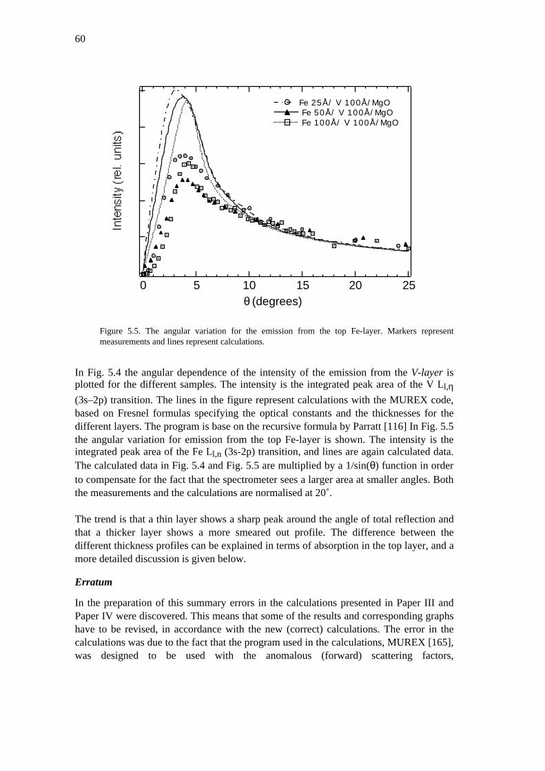
60

2520151050 θ (degrees)

Fe 25Å/ V 100Å/MgO Fe 50Å/ V 100Å/MgO Fe 100Å/ V 100Å/MgO

Figure 5.5. The angular variation for the emission from the top Fe-layer. Markers representmeasurements and lines represent calculations.

In Fig. 5.4 the angular dependence of the intensity of the emission from the V-layer isplotted for the different samples. The intensity is the integrated peak area of the V Ll,η(3s–2p) transition. The lines in the figure represent calculations with the MUREX code,based on Fresnel formulas specifying the optical constants and the thicknesses for thedifferent layers. The program is base on the recursive formula by Parratt [116] In Fig. 5.5the angular variation for emission from the top Fe-layer is shown. The intensity is theintegrated peak area of the Fe Ll,n (3s-2p) transition, and lines are again calculated data.The calculated data in Fig. 5.4 and Fig. 5.5 are multiplied by a 1/sin(θ) function in orderto compensate for the fact that the spectrometer sees a larger area at smaller angles. Boththe measurements and the calculations are normalised at 20˚.

The trend is that a thin layer shows a sharp peak around the angle of total reflection andthat a thicker layer shows a more smeared out profile. The difference between thedifferent thickness profiles can be explained in terms of absorption in the top layer, and amore detailed discussion is given below.

Erratum

In the preparation of this summary errors in the calculations presented in Paper III andPaper IV were discovered. This means that some of the results and corresponding graphshave to be revised, in accordance with the new (correct) calculations. The error in thecalculations was due to the fact that the program used in the calculations, MUREX [165],was designed to be used with the anomalous (forward) scattering factors,

61

f 0 = Z + ′ f (ω ) − i ′ ′ f (ω) , as parameters, whereas we used the atomic (forward)

scattering factors, f 0 = f1 − if2 , given in the tabulations by Henke et al. [30], seeChapter 2. This results in an error in the real part of the refractive index, 1–δ, used in thecalculations. The corrected results are given in Fig. 5.4 and Fig. 5.5 . In Fig. 5.2 onlymeasurement data are presented.

Since the measurements and the calculations were normalised with respect to the peakstructure corresponding to the critical angle, θc, which is affected by a change in δ, the

measurement data presented in Paper III and Paper IV are given with an incorrect anglescale. The angles given here in the corrected Fig. 5.4 and Fig. 5.5 are the anglesestimated from intensity to be the correct absolute values. The error in the measuredabsolute angle is estimated to be within ± 2˚. The other difference is that the ratiobetween β and δ changes, which means that the forms of the curves are changed slightly.This, however, does not change the qualitative results and the calculations are now foundto agree much better with the measurements.

5.3 Discussion

The angular dependence can be discussed in terms of the different optical constants forthe different layers and application of Fresnel formulas.

Reflection and transmission

At x-ray frequencies the phase velocity of electromagnetic radiation exceeds c by a smallamount, since n < 1. Thus an x-ray wave will increase its wavelength when passing aninterface from vacuum to another solid material. When the angle to the substratebecomes very small, so that the direction of the incoming beam is almost parallel to thesurface, the phases of the shorter wavelength vacuum wave and the longer wavelengthwave in the medium can no longer match along the interface. The only way of matchingis then an exponentially damped, evanescent wave in the medium, propagating along theinterface but exponentially damped perpendicular to the interface. This is reflected inSnell's law which describes the phase matching between the different waves in aquantitative way.

Snell's law relates the incoming and refracted angles and can be derived from the phasematching at the interface, see Fig 5.6:

ki,x = kt ,x ⇒ 1 ⋅ cos(θ ) = n ⋅ cos(θt ) (5.1)

from which we can derive the following relation

nsin(θt) = n2 − cos2θ . (5.2)

62

Here θ is the grazing angle of incidence and ki,z = ki sin(θ) and kt,z = kt sin(θt) are the

perpendicular components of the wavevector of the incident and transmitted waves, seeFig. 5.6.

The reflection and transmission at a perfectly smooth interface are given by the well-known Fresnel formulas [26], based on Maxwell's formulas and the continuity of the Eand H fields across an interface. The Fresnel amplitude transmission and reflectionfactors which are related to the fields on either side of the surface are given for the caseof a plane wave in vacuum impinging on a medium with refractive index n:

ts = Et

Ei=

2ki,z

ki,z + kt ,z= 2sinθ

sinθ + n2 − cos2 θ

rs = Er

Ei=

ki ,z − kt,z

ki ,z + kt ,z= sinθ − n2 − cos2 θ

sinθ + n2 − cos2 θ

(5.3)

where we have used Snell's law, Eq. (5.2), in the second step. The case for polarisationperpendicular to the plane of refraction (s-polarisation)12 is given here. The relations forparallel polarisation, p-polarisation, are similar and can be found for instance in [26].Since n is almost unity for x-rays, in practice there is very little difference between the sand p-polarised cases, and in the following only the s-polarised case is considered.

Figure 5.6. Schematic picture of the reflection and transmission at an interface between vacuum anda medium with n < 1 for the case of s-polarisation.

The Fresnel reflection factor, Rs = rs2 , and the Fresnel transmission factor, Ts = ts

2 are

shown in Fig. 5.7 and Fig. 5.8 respectively for various β/δ ratios. Rs shows the expectedtotal reflection below the critical angle of total reflection, θc, given by cos(θc) = n fromSnell's law. It is seen that the reflection is less than total for finite β, and that for β/δ = 1,the total reflection effect has disappeared. The transmission factor shows a pronouncedmaximum for angles around θc. This is related to the fact that the reflected and

transmitted waves add in phase at this angle, since the phase shift for the reflected waveis zero for reflection against an optically less dense medium (for the case of β ≈ 0) [119].This peak in the transmittance is, as we shall see, important for the angular properties of

12 s is from the German word senkrecht meaning perpendicular or vertical, c. f. Swedish sänke, lod.

63

x-ray emission for grazing exit angles around θc. This is the background to the prominent

peak close to the critical angle. It should be noted though that Fig. 5.8 does not show theenergy transmittance, and an analysis using the Poynting vectors shows that the energy isconserved, so that the energy transmittance still does not exceed unity.

1.0

0.8

0.6

0.4

0.2

0.0

3.02.52.01.51.00.50.0

Θ/Θc

β/δ = 0 β/δ = 1/50 β/δ = 1/10 β/δ = 1/5 β/δ = 1

Figure 5.7. The reflectance for grazing angles around the critical angle of reflection for differentratios of β and δ.

4

3

2

1

0

3.02.52.01.51.00.50.0

Θ/Θc

β/δ = 0 β/δ = 1/50 β/δ = 1/10 β/δ = 1/5 β/δ = 1

Figure 5.8. The Fresnel transmission factor for grazing angles around the critical angle of reflectionfor different ratios of β and δ.

Angular dependence—calculations

The angular dependence of the emission can be explained by looking at the reciprocalsituation, namely the grazing incidence case, where the transmission from a wave invacuum into the medium is considered. As was mentioned earlier, Becker et al. verifiedthis approach experimentally [147]. The calculations are then carried out as if an

64

absorption experiment had been carried out, considering an imaginary source at theposition of the detector. Assuming a plane wave incident on the sample, the field inside amultilayer can be calculated using recursion formulas [116]. The program used in ourstudies, MUREX [165], uses such an approach. There is an approximation in therecursion formulas for small angles, sin(θ) ≈ θ, which can be justified up to about 15˚,but is a source of errors above that angle. However, this should not affect the resultsqualitatively since the most interesting range is below 15˚.

Below the critical angle of total reflection the refracted angle, θt, becomes imaginary

corresponding to an imaginary k in the z-direction:

kz =2πλ

nsin(θt) =2πλ

n2 − cos2(θ)

where the last step follows from Snell's law, Eq. (5.2). Since the critical angle is given bycos(θc ) = n , it follows directly that kz is imaginary for θ < θc. This imaginary k

corresponds to an evanescent wave that propagates along the interface but isexponentially damped in the z-direction. This means that a wave impinging on thesurface at a smaller grazing angle than θc will penetrate only the evanescent wave region,

corresponding to a depth of about 50 Å in the wavelength range used here. In an idealcase without damping, β = 0, the evanescent wave, will not transport any energy in the z-direction, and this is also seen in the total reflection properties, Fig. 5.7. For finite β,however, energy will be dissipated in the evanescent field so that kz will have also a real

part, and there will be a finite energy transport in the z-direction [13]. This is also seen inthe reflectance properties, see Fig. 5.7, in that the reflectance is less than total below θcfor finite β.

The reciprocity theorem now states that the grazing incidence and grazing exit cases aresimilar so that for an exit angle below θc only emission from a layer corresponding to the

evanescent wave region is seen by the detector. Thus, the penetration depth in the grazingincidence case and the information depth in the grazing exit case are the same.

From the plane wave equation, E = E0ei(kr−ωt ) , it can be seen that the intensity decays as

I = I0e−2Im(k z )z .

and from this equation it is seen that the depth at which the intensity has decreased to 1/etimes the intensity at the surface is given by

z1 /e =1

2 I m (kz ), (5.4)

that is, the 1/e penetration depth.

For small angles, θ ≈ 0˚, the penetration depth, Eq. (5.4) is given by the decay of theevanescent field in the medium and becomes approximately,

65

z1 /e (0) ≈λ

2π 2δ= δ =

2πλ

reNat f1

=

const

Nat f1

where the definitions are as given in Chapter 2. The penetration depth for the evanescentwave thus becomes smaller for higher density and larger f1. Typical values are found inFig. 5.9 for the case of vanadium and iron to be around 40 Å. As f1 can bee seen as thenumber of effective free electrons at a certain wavelength it follows that, Natf1 ≈ Neff. el.,

the number of effective electrons per unit volume. The penetration depth for theevanescent wave region can thus be interpreted as an effective screening length for thefield, similar to the Debye screening length [12].

10

2

4

6

8100

2

4

6

81000

20151050

θ (degrees)

Vanadium Iron sin(θ)/µ

θc

Figure 5.9. The penetration/information depth vs. angle. The case of vanadium and iron at awavelength 27.8 Å (V Ll) is shown.

For larger grazing angles, the penetration depth is given by the linear attenuation

(absorption) coefficient, µ =4πβλ

. The penetration at normal incidence is thus given by

the linear absorption length

z1 /e (90˚) =1

µ=

λ4πβ

.

At large angles, θ >> θc , the penetration depth is to a good approximation given by the

geometrical projection of the linear absorption length:

z1 /e (θ) ≈sinθ

µ(5.5)

66

This approximation is valid as long as refraction can be neglected as is seen from the useof the incidence angle, θ, in the expression. For illustration, Eq. (5.5) is plotted togetherwith the correct expression, Eq. (5.4), in Fig. 5.9. From this example it is seen that Eq.(5.5) is a valid approximately for angles, θ ≥ 3θc , i. e. for these angles refraction effectscan approximately be neglected. We briefly mention that the penetration depth at θ = θc

can be shown to be given by [13] z1 /e (θc) ≈ λ2π β

.

Angular intensity profiles

Neglecting multiple reflections, the intensity of emission generated in a surface layerranging from z=z0 to z=z0+d is given by [149]

I(θ) = const ⋅ t 2e−2Im( kz )(z−z0 )ps(z)dzz0

z0 +d

∫ (5.6)

where ps(z) is the emission intensity at depth z. The two first factors in this integral is

ts2 , the Fresnel transmission factor for the surface interface and e−2Im(kz )(z−z0 ) ,

corresponding to the attenuation of radiation generated at a depth z along its path to thesurface, z0. In the derivation of Eq. (5.6), Urbach and de Bokx [149] considered thedirect problem of a source in a thin layer and the detector in vacuum, and usedasymptotical plane wave expansions for the solution.

It is somewhat surprising that the factor ts2 , the Fresnel transmittance factor for

refraction from vacuum into the medium, is involved in the result and not thetransmission factor from the medium into vacuum. As has been pointed out [149] theoccurrence of this factor in the solution of the direct problem is an illustration of thereciprocity theorem. In Eq. (5.6) multiple reflection effects was not considered. If theabsorption in the layer is not too high there will also be interference effects due tomultiple reflections at the interfaces which should then also be taken into account.

The multiple reflection effects are actually illustrated by the results in the emission fromthe V-layer, Fig. 5.4 since the peak at 4.5˚ corresponds to the angle of total reflection ofthe MgO-substrate. This is possible since the V-layer has a slightly larger index ofrefraction than the MgO-layer for the wavelength used. This was simulated withcalculations, using different values of the index of refraction for the MgO-substrate sothat the total reflection angle changes. The peak then changes position and disappears forrefractive indices equal to or larger than the refractive index for V.

67

3.02.52.01.51.00.50.0Θ/Θc

25 Å 100 Å 500 Å 1000 Å

β/δ = 0.01

3.02.52.01.51.00.50.0Θ/Θc

25 Å 100 Å 500 Å 1000 Å

β/δ = 0.2

Figure 5.10. Illustration of the angular variation of the emission from layers of different thicknessfrom MUREX calculations. The data is presented relatively to the critical angle and are normalisedat θ = 3θc. Left and right panels show different ratio between β and δ.

The influence of β on the angular emission profile is shown in Fig. 5.10 wherecalculations are shown for layers of varying thickness and for β/δ = 0.01, left panel, andβ/δ = 0.2, right panel. The differences are an effect of the difference in self absorption fordifferent β. This can be seen by comparing with the penetration depth in Fig. 5.9.Another interesting feature is the differences between different depths in the case withoutabsorption. For larger depths, less of the "tunnelling" phenomenon, the emission forangles less than θc, is seen This corresponds to a larger fraction of the emission coming

from depths larger than the evanescent wave penetration depth. Fig. 5.10 can becompared with the results presented in Fig. 5.4 and 5.5. For instance the case of 100 Å inFig. 5.4 shows the influence of the absorption in the Fe-layer that is on top. Thevariations in Fig 5.5 for different top layer thickness show the same trends as in Fig.5.10, left panel.

5.4 Summary

In summary the angular variation properties in soft x-ray emission can be seen as thereciprocal of the reflection properties; a small grazing angle corresponds to highreflection and a short penetration depth into the sample—this then corresponds,reciprocally, to a small information depth in emission.

The variation in information depth can, in principle, be used for depth profiling, althoughthe information depth changes very rapidly with angle around θc, so a high angular

resolution is then needed. As we have seen, Figs. 5.4, 5.5 and 5.10, there are differentangular profiles for different thicknesses, depending essentially on the absorption in thelayer, or in the layers above. This suggests that the angular profile could be used formeasurement of β for a known thickness. Since the peak position depends essentially onthe critical angle, θc = 2δ , one could also think of using angular resolved emission as a

68

method for determining δ, complementary to or instead of reflection measurements. Thesame deficiencies as with reflection measurements such as the influence of surfaceroughness and surface contamination are likely to be present in emission since the peakstructure around θc is largely dependent on the sample/vacuum interface (i. e. the

surface) properties.

For a wavelength dispersive instrument, such as the concave grating instrument we haveused, with a relatively small angle of acceptance, it is furthermore an advantage to usegrazing exit angles in that the match between the spectrometer acceptance and the spotsize in most cases becomes better. As an example, the instrument we have used typicallyhas an acceptance angle of 7 mrad. If the sample-slit distance is 20 mm, the spectrometerthen "sees" a spot size of 0.15 mm. If the electron beam excites a spot of 1 mm, thesample should be tilted to a grazing exit angle of 0.15 rad ≈ 8.5˚ for the spectrometer tosee the whole spot.13 Another way of obtaining matching with the spectrometeracceptance is to use a microfocused electron beam (or photon beam) for excitation. Whenusing electron excitation, a more spread out excitation can sometimes be advantageous,however, since this decreases the risk for sample damage. For intensity reasons alone it isalso interesting to note that the intensity is highest around θc.

13 In our studies we used a smaller angular acceptance of 0.12˚ for angular resolution reasons, and a spotsize of approximately 4 mm, corresponding to an optimum tilt angle as low as 10 mrad ≈ 0.6˚.

6 ALUMINIUM AND NICKEL OXIDE FILMS STUDIEDWITH SOFT X-RAY SPECTROSCOPY

6.1 Anodised aluminium oxide

In Paper V, some results on anodised aluminium oxide films are presented.

Aluminium oxide films have important technical applications. They can be used asprotective coatings on reflector plates and porous aluminium oxide films can be used as amatrix for metallic particles with the application as selective coatings for solar absorbers.

In this study the Al Lα,β emission from different Al2O3 coatings, non-porous, porous and

Ni-pigmented porous were compared. Both synchrotron radiation and electron emissionexcitation were used. Since the Al Lα,β emission spectra in Al2O3 and Al are

characteristically different, the emission spectra can give information about the chemicalstate of aluminium. The different samples show different character. The non-porous andthe Ni-pigmented samples show oxide character, whereas the porous oxide film shows asuperposition of oxide and metallic character. Measurements at different exit anglesshow that the metallic Al-signal either comes from the substrate or from deep-lyingparticles in the film. Different possibilities such as an enhanced substrate signal by oxidepores acting as waveguides are discussed.

6.2 Nickel oxide for electrochromic applications

In this section some preliminary results on x-ray absorption studies of NiO will bepresented.

XAS was used to study reactively sputtered NiO-films [166] for electrochromicapplications. The films are polycrystalline and have a relatively small grain size (about20 nm) as shown from x-ray diffraction measurements [166,167]. The films are sputteredon glass substrates precoated with a conductive ITO-layer. The film thickness is about200 nm.

Two different samples were compared; one sample which was highly absorbing in thevisible, here called coloured, and one almost transparent in the visible, here called

70

transparent. The coloured sample was prepared by exposing the sputtered film to UV-light in air atmosphere. The UV-light produces some ozone, which is suspected to reactwith the film. Especially, reactions are suspected to take place at the grain boundaries.The transparent samples were prepared by exposing the deposited films to UV-light inAr-atmosphere [167].

The absorption measurements were carried out at MAX-lab, beamline I511, using totalelectron yield (TEY) and photon yield (FY) techniques, see Chapter 3. The TEY-measurements were performed by measuring the sample current from the conductiveITO-layer, and the FY measurements by using a channeltron with a negative bias voltageto repel electrons. As was mentioned in section 2.1, XAS probes the unoccupied LPDOS.It should be noted however, that there is a core-hole in the final state, and we aretherefore not probing the ground state.

The results are presented in Fig. 6.1 and Fig. 6.2. Absorption scans of the O K-absorptionedge is shown in Fig. 6.1 and scans of the Ni L-edge in Fig. 6.2. The measurements arenormalised to the incoming intensity.

570560550540530520

Photon energy (eV)

NiO_transp_O1s_TFYNiO_coloured_O1s_TFYNiO_transp_O1s_TEY NiO_coloured_O1s_TEY

Figure 6.1. Fluorescence yield (TFY) and electron yield (TEY) measurements of the O K-absorption edge.

71

880875870865860855850845

Photon energy (eV)

NiO_Coloured_Ni2p_TEY

NiO_Transp_Ni2p_TEY

Figure 6.2. Total electron yield measurements of the Ni L-edge.

The most prominent feature in the spectra is the pre-peak at 528 eV in the O absorptionspectra, Fig 6.1. This peak is present in the coloured sample, but not in the transparentsample. Similar XAS-spectra for NiO doped with Li has been presented [168]. In thissystem the charge compensating holes are mainly of O 2p character. A possibleinterpretation for our samples is that the coloured films are slightly over-stoichiometric,where the reactions are suspected to take place at the grain boundaries. If this is the case,the excess oxygen introduce holes, or unoccupied electronic states, in the valence band ofO 2p character. These empty states are probably also related to the colouring in thevisible.

The spectra in Fig. 6.2 do not show such large differences between the two samples, butthe spectra can be compared with similar Ni absorption spectra of Li-doped NiO [169]which show changes in the same direction.

The present analysis is very preliminary and a more thorough discussion will follow in aforthcoming publication.

7 CONCLUDING REMARKS

In this thesis, various applications of soft x-ray spectroscopy have been presented. Instudies of deposition processes it is shown to be a valuable tool for analysing the growingfilm in-situ. The method provides both elemental and chemical information and isrelatively insensitive to electric and magnetic fields and can therefore be used in-situduring sputter deposition. For example, different stoichiometric phases of a compoundcan be identified and monitored in-situ.

By varying the angle of detection in emission spectroscopy, depth information can beobtained. At small grazing exit angles, for example, only emission from the surface layeris probed. The variation in information depth can, in principle, be used for depthprofiling, although the information depth changes very rapidly with angle, so that highangular resolution is needed to obtain such information.

The surface sensitivity of soft x-ray emission spectroscopy in grazing exit can be of greatinterest per se, for instance in studies of thin film growth. For studies of depositionprocesses it is of obvious importance to be surface sensitive when monitoring thedeposition process. The probe depth of the analysis technique should preferably besmaller or at least of the same order as the film deposition rate. The time scale forfeedback is then short and the analysis method can be used for real-time monitoring ofthe film growth, and even as feedback for controlling the process; perhaps not forcontrolling the reactive sputtering process as such, but when choosing the correctworking point. Further development is needed for actually applying the SXES in-situduring deposition, but since it actually probes the growing film the method has a greatpotential for such applications.

Soft x-ray spectroscopy was also applied for studies of anodised Al2O3 films for solarabsorber applications and for studies of electrochromic NiO-films. The results from thex-ray absorption studies of electrochromic NiO show the potential of the method forstudying the electronic structure of these materials.

73

Acknowledgements

First I would like to thank my supervisors: Claes-Göran Granqvist, for your patience andsupport and for helping me see the possibilities instead of the problems. Arne Roos, forhelping me to get to the point where I am now. Your comments, careful reading and greathelpfulness have been invaluable to me.

I am very grateful to Jan-Erik Rubensson for his enthusiasm, for showing such greatinterest in my work and for many interesting scientific discussions. Thanks also for manyvaluable comments on my manuscript and for carrying on the "last-night tradition".Many thanks to all my co-workers, especially Per Skytt, who taught me the experimentalbusiness, and Tanel Käämbre, the hard-working guy, for great help with many things andfor never giving up. Tomas Nyberg is thanked for answering all my sputtering questions.Joseph Nordgren is thanked for giving me the opportunity to work in the field of soft x-ray spectroscopy and C-G Ribbing, a truly good teacher, for introducing me to solid statephysics and to the field of sputtering and soft x-ray spectroscopy. Thanks also to: AndrisAzens for help with preparing samples; Roberta Roos, for help with proof reading themanuscript; Esbjörn, for help with many practical matters and for valuable commonsense; Tuquabo, for help with editing and for being such a nice fellow. I wish you all thebest "Down under".

All colleagues and friends, former and present, at the solid state physics group arethanked for the social activities and for providing a nice environment to work in. At therisk of forgetting someone, I especially mention, Monica, Monika, Richard, Ewa,Annette, Jan, Jacob, Per and Lisen. All members of the soft x-ray group are also greatlyacknowledged.

Finally I would like to mention my wife and children, who had to put up with myabsence for a long time:Maria—without all your support this thesis would not have been completed!Max and Moa—next winter there will certainly be more time for skiing!

Uppsala, March 2001

Björn Gålnander

REFERENCES

1. G. Landwehr in Röntgen Centennial: X-rays in Natural and Life Sciences, Eds. A.Haase, G. Landwehr, and E. Umbach, (World Scientific, 1997).

2. A. Pais, Inward Bound (Oxford University Press, Oxford, 1986).

3. M. Siegbahn, Spektroskopie der Röntgenstrahlen , 2, (Springer, Berlin, 1931).

4. H. M. O'Bryan and H. W. B. Skinner, Phys. Rev. 44, 602 (1933).

5. H. M. O'Bryan and H. W. B. Skinner, Phys. Rev. 45, 370 (1934).

6. H. W. B. Skinner, Phil. Trans. Roy. Soc. London A 239, 95 (1940).

7. B. H. Bransden and C. J. Joachain, Physics of Atoms and Molecules (Longman,Harlow, 1983).

8. C.-O. Almbladh and L. Hedin in Handbook on Synchrotron Radiation, Vol 1, Ed. E.E. Koch, (North-Holland, Amsterdam, 1983).

9. D. J. Fabian, Ed. Soft X-Ray Band Spectra (Academic Press, London, 1968)

10. R. Manne, J. Chem. Phys. 52, 5733 (1970).

11. H. Jones, N. F. Mott, and H. W. B. Skinner, Phys. Rev. 45, 379 (1934).

12. J. D. Jackson, Classical Electrodynamics , 3rd ed., (Wiley, New York, 1998).

13. D. Attwood, Soft X-rays and Extreme Ultraviolet Radiation: Principles andApplications (Cambridge University Press, Cambridge, 2000).

14. A. H. Compton and S. K. Allison, X-Rays in Theory and Experiment , 2nd. ed.,(Van Nostrand, New York, 1935).

15. F. Wooten, Optical Properties of Solids (Academic Press, New York, 1972).

16. H. A. Kramers and W. Heisenberg, Z. Physik 31, 681 (1925).

17. J. J. Sakurai, Advanced Quantum Mechanics (Addison-Wesley, Redwood City, CA,1985).

18. W. Heitler, The Quantum Theory of Radiation (Dover, New York, 1984).

19. I. Waller, Phil. Mag. 4, 1228 (1927).

20. P. W. Atkins and R. S. Friedman, Molecular Quantum Mechanics , 3, (OxfordUniversity Press, Oxford, 1997).

21. Special issue "RIXS", Applied Physics A 65 (1997).

22. F. Gel'mukhanov and H. Ågren, Physics Reports 312, 87 (1999).

23. E. Hecht, Optics , 3rd. ed., (Addison-Wesley, Reading, MA, 1998).

24. P. P. Ewald, Ann. der Physik 49, 1 (1917).

75

25. W. Oseen, Ann. der Physik 48, 1 (1915).

26. M. Born and E. Wolf, Principles of Optics (Pergamon, Oxford, 1993).

27. D. W. Oxtoby, F. Novak, and S. A. Rice, J. Chem. Phys. 76, 5278 (1982).

28. C. G. Darwin, Phil. Mag. 27, 315 (1914).

29. R. W. James, The Optical Principles of the Diffraction of X-Rays (Bell, London,1967).

30. B. Henke, E. M. Gullikson, and J. C. Davis, At. Data Nucl. Data Tables 54, 181(1993).

31. H. C. van de Hulst, Light Scattering by Small Particles (Dover, New York, 1981).

32. C. F. Bohren and D. R. Huffman, Absorption and Scattering of Light by SmallParticles (Wiley, New York, 1983).

33. R. G. Newton, Am. J. Phys. 44, 639 (1976).

34. E. Spiller, Applied Optics 29, 19 (1990).

35. D. Y. Smith and J. H. Barkyoumb, Phys. Rev. B 41, 11529 (1990).

36. A. H. Compton, Phys. Rev. 20, 84 (1922).

37. A. Larsson, M. Siegbahn, and I. Waller, Naturwiss. 12, 1212 (1924).

38. K. Grandin, Ph. D. Dissertation, Uppsala University, 1999.

39. A. Larsson, Ph. D. Dissertation, Uppsala University, UUÅ, 1929.

40. W. K. Warburton and K. F. Ludwig, Phys. Rev. B 33, 8424 (1986).

41. E. D. Palik, Ed. Handbook of Optical Constants of Solids (Academic Press,Orlando, 1985)

42. E. D. Palik, Ed. Handbook of Optical Constants of Solids II (Academic Press, SanDiego, CA, 1991)

43. D. W. Lynch in Handbook on Synchrotron Radiation, Ed. G. V. Marr, Vol. 2,(North-Holland, Amsterdam, 1987).

44. B. Lengeler in Resonant Anomalous X-Ray Scattering, Eds. G. Materlik, C. J.Sparks, and K. Fischer, (North-Holland, Amsterdam, 1994).

45. D. C. Creagh and W. J. McAuley in International Tables for Crystallography, Vol.C, Ed. A. J. C. Wilson, (Kluwer, Dordrect, 1992).

46. D. C. Creagh, Rad. Phys. Chem. 56, 61 (1999).

47. J. Barth, R. L. Johnson, and M. Cardona in Handbook of Optical Constants ofSolids II, Ed. E. D. Palik, (Academic Press, San Diego, CA, 1991).

48. J. Pflüger and J. Fink in Handbook of Optical Constants of Solids II, Ed. E. D.Palik, (Academic Press, San Diego, CA, 1991).

49. H. G. Birken, C. Blessing, and C. Kunz in Handbook of Optical Constants of SolidsII, Ed. E. D. Palik, (Academic Press, San Diego, CA, 1991).

76

50. B. L. Henke, Phys. Rev. A 6, 94 (1972).

51. D. C. Creagh in International Tables for Crystallography, Vol. C, Ed. A. J. C.Wilson, (Kluwer, Dordrecht, 1992).

52. E. B. Saloman, J. H. Hubbell, and J. H. Scofield, At. Data Nucl. Data Tables 38, 1(1988), See also the www-page: physics.nist.gov/PhysRefData.

53. J. J. Yeh and I. Lindau, At. Data Nucl. Data Tables 32, 1 (1985).

54. N. K. Del Grande, Physica Scripta 41, 110 (1990).

55. R. Soufli and E. M. Gullikson, Applied Optics 37, 1713 (1998).

56. H. J. Hagemann, W. Gudat, and C. Kunz, J of Opt. Soc. Am. 65, 742 (1975).

57. R. L. Blake, J. C. Davis, D. E. Graessle, T. H. Burbine, and E. M. Gullikson inResonant Anomalous X-Ray Scattering, Eds. G. Materlik, C. J. Sparks, and K.Fischer, (North-Holland, Amsterdam, 1994).

58. R. Soufli and E. M. Gullikson, Applied Optics 36, 5499 (1997).

59. J. Svatos, D. Joyeux, D. Phalippou, and F. Polack, Optics Letters 18, 1367 (1993).

60. R. Tatchyn in Handbook of Optical Constants of Solids II, Ed. E. D. Palik,(Academic Press, San Diego, CA, 1991).

61. U. Bonse and M. Hart, Appl Phys. Lett 7, 238 (1965).

62. www-cxro.lbl.gov

63. J. Stöhr, NEXAFS Spectroscopy (Springer-Verlag, New York, 1992).

64. B. L. Henke, Nucl. Instr. Meth. 177, 161 (1980).

65. E. Bäcklin, Z. Physik 93, 450 (1934).

66. M. Siegbahn and T. Magnusson, Z. Physik 62, 435 (1930).

67. See manufacturers of holographic ion-etched gratings such as Spectrogon,www.spectrogon.com or Jobin-Yvon, www.jobinyvon.com

68. H. A. Rowland, Phil. Mag. 13, 469 (1883).

69. R. A. Sawyer, Experimental Spectroscopy (Chapman & Hall, London, 1944).

70. J. A. R. Samson, Techniques of Vacuum Ultraviolet Spectroscopy (PiedPublications, Lincoln, 1967).

71. J. E. Mack, J. R. Stehn, and B. Edlén, J of Opt. Soc. Am. 22, 245 (1931).

72. R. J. Speer, Space Science Instrumentation 2, 463 (1976).

73. J. Nordgren, G. Bray, S. Cramm, R. Nyholm, J.-E. Rubensson, and N. Wassdahl,Rev. Sci. Instr. 60, 1690 (1989).

74. J. Nordgren and R. Nyholm, Nucl. Instr. Methods A 246, 242 (1986).

75. L. Duda, Ph. D. Dissertation, Uppsala University, 1996.

76. M. Gryzinski, Phys. Rev. 138, A 336 (1965).

77

77. G. Wiech in X-ray emission spectroscopy, Ed. P. Day, 103, (D. Reidel PublishingCompany, 1981).

78. J. Electron Spectrosc. Relat. Phenom. 110-111 (2000).

79. W. A. Hendrickson, Science 254, 51 (1991).

80. R. Kahn, P. Carpentier, C. Berthet-Colominas, and M. Capitan, J. Synchrotron Rad.7, 131 (2000).

81. G. Schütz, M. Knülle, and H. Ebert in Resonant Anomalous X-Ray Scattering, Eds.G. Materlik, C. J. Sparks, and K. Fischer, (North-Holland, Amsterdam, 1994).

82. T. Eimüller, P. Fischer, G. Schütz, P. Guttman, G. Schmal, K. Pruegl, and G.Bayreuther, J. of Alloys Comp. 286, 20 (1999).

83. J. Jaklevic, J. A. Kirby, M. P. Klein, A. S. Robertson, G. S. Brown, and P.Eisenberger, Solid State Commun. 23, 679 (1977).

84. S. Eisebitt, T. Böske, J.-E. Rubensson, and W. Eberhart, Phys. Rev. B 47, 14103(1992).

85. J. L. Vossen and W. Kern, Eds., Thin Film Processes II (Academic Press, SanDiego, 1991)

86. R. Gordon, Journal of Non-Crystalline Solids 218, 81 (1997).

87. T. Tesfamichael, Ph. D. Dissertation, Uppsala University, 2000.

88. B. Chapman, Glow Discharge Processes (Wiley, San Diego, 1980).

89. D. A. Glocker and S. I. Shah, Eds., Handbook of Thin Film Process Technology(IOP Publishing, Bristol, 1995)

90. L. I. Maissel and R. Glang, Eds., Handbook of Thin Film Technology (Mc GrawHill, New York, 1970)

91. T. Nyberg, Ph. D. Dissertation, Uppsala University, 1997.

92. W. Wasa and S. Hayakawa, Handbook of Sputter Deposition Technology (Noyes,Park Ridge, NJ, 1992).

93. P. Sigmund in Sputtering by Particle Bombardment I, Ed. R. Behrisch, Topics inApplied Physics, Vol. 47, (Springer, Berlin, 1981).

94. S. I. Shah in Handbook of Thin Film Process Technolgy, Eds. S. I. Shah and D. A.Glocker, (IOP Publishing, Bristol, 1995).

95. J. M. Schneider and W. D. Sproul in Handbook of Thin Film Process Technology,Eds. S. I. Shah and D. A. Glocker, (IOP Publishing, Bristol, 1998).

96. M. I. Ridge and R. P. Howson, Thin Solid Films 96, 121 (1982).

97. W. D. Sproul, Thin Solid Films 107, 141 (1983).

98. A. Skerlavaj, Y. Claesson, and C.-G. Ribbing, Thin Solid Films 186, 15 (1990).

78

99. T. Larsson, H.-O. Blom, C. Nender, and S. Berg, J. of Vac. Sci. Technol. A 6, 1832(1987).

100. R. P. Howson, A. G. Spencer, K. Oka, and R. W. Lewin, J. of Vac. Sci. Technol. A7, 1230 (1989).

101. T. Nyberg, C. Nender, and S. Berg, J. of Vac. Sci. Technol. A 16, 1868 (1998).

102. J. Chapin and C. R. Condon, US Patent No: 4,116,784 (1979).

103. S. Berg, H.-O. Blom, M. Moradi, and C. Nender, J. of Vac. Sci. Technol. A 7, 1225(1989).

104. S. Berg, T. Larsson, and H.-O. Blom, J. of Vac. Sci. Technol. A 4, 594 (1986).

105. S. Berg, H.-O. Blom, T. Larsson, and C. Nender, J. of Vac. Sci. Technol. A 5, 202(1987).

106. S. Berg, T. Larsson, C. Nender, and H.-O. Blom, J. Appl. Phys. 63, 887 (1988).

107. H. Sekiguchi, A. Kanzawa, T. Imai, and T. Honda, J. of Vac. Sci. Technol. A 12,3176 (1994).

108. M. Moradi, C. Nender, H.-O. Blom, and S. Berg, Vacuum 41, 1974 (1990).

109. M. Moradi, C. Nender, S. Berg, H.-O. Blom, A. Belkind, and Z. Orban, J. of Vac.Sci. Technol. A 9, 619 (1991).

110. P. Carlsson, C. Nender, H. Barankova, and S. Berg, J. of Vac. Sci. Technol. A 11,1534 (1993).

111. S. Berg, T. Nyberg, H.-O. Blom, and C. Nender in Handbook of Thin Film ProcessTechnology, Eds. S. I. Shah and D. A. Glocker, (IOP Publishing, Bristol, 1998).

112. M. Georgson, G. Bray, Y. Claesson, J. Nordgren, C.-G. Ribbing, and N. Wassdahl,J. of Vac. Sci. Technol. A 9, 638 (1991).

113. M. J. Romand, F. Gaillard, and M. Charbonnier, Adv. in X-Ray. Anal. 35, 819(1992).

114. P. B. Legrand, J. P. Dauchot, M. Hecq, M. Charbonnier, and M. Romand, J. of Vac.Sci. Technol. A 12, 1551 (1994).

115. P. Skytt, C.-J. Englund, N. Wassdahl, D. Mancini, and J. Nordgren, Proc. SPIE2283, 141 (1994).

116. L. G. Parratt, Phys. Rev. 95, 359 (1954).

117. S. K. Sinha, E. B. Sirota, S. Garoff, and H. B. Stanley, Phys. Rev. B 38, 2297(1988).

118. K. N. Stoev and K. Sakurai, Spectrochimica Acta B 54, 41 (1999).

119. M. Tolan, X-Ray Scattering from Soft-Matter Thin Films (Springer, Berlin, 1999).

120. V. Holy, U. Pietsch, and T. Baumbach, High-Resolution X-Ray Scattering fromThin Films and Multilayers (Springer, Berlin, 1999).

79

121. P. H. Fuoss, K. S. Liang, and P. Eisenberger in Synchrotron Radiation Research:Advances in Surface and Interface Science, Ed. R. Z. Bachrach, Vol. 1, (PlenumPress, New York, 1992).

122. H. Zabel, Appl. Phys. A 58, 159 (1994).

123. E. Spiller, Proc. SPIE 563, 367 (1985).

124. J. B. Kortright, J. Appl. Phys. 70, 3620 (1991).

125. E. Spiller, D. Stearns, and M. Krumrey, J. Appl. Phys. 74, 107 (1993).

126. E. M. Gullikson and D. G. Stearns, Phys. Rev. B 59, 13273 (1999).

127. W. C. Marra, P. Eisenberger, and A. Y. Cho, J. Appl. Phys. 50, 6927 (1979).

128. G. H. Vineyard, Phys. Rev. B 26, 4146 (1982).

129. P. L. Cowan, Phys. Rev. B 32, 5437 (1985).

130. M. F. Toney, T. C. Huang, S. Brennan, and Z. Rek, J. Mater. Res 3, 351 (1988).

131. J. Luo, K. Tao, H. Yin, and Y. Du, Rev. Sci. Instr. 67, 2859 (1996).

132. I. Szalóki, B. T. Szabina, R. Chul-Un, J. Injuk, and R. E. Van Grieken, Anal. Chem.72, 211R (2000).

133. R. Klockenkämper, Total-Reflection X-Ray Fluorescence Analysis (Wiley, NewYork, 1997).

134. Manufacturers of equipment e g www.atomika.com

135. Beamline ID 27 at ESRF, www.esrf.fr/exp_facilities/ID27

136. F. Comin, M. Navizet, P. Mangiagalli, and G. Apostolo, Nucl. Inst. Methods B 150,538 (1999).

137. K. Sakurai, Spectrochimica Acta B 54, 1497 (1999).

138. D. K. G. de Boer, Phys. Rev. B 44, 498 (1991).

139. K. Sakurai and A. Iida, Adv. in X-Ray. Anal. 39, 695 (1997).

140. P. L. Cowan, J. A. Golovchenko, and M. F. Robbins, Phys. Rev. Lett. 44, 1680(1980).

141. M. J. Bedzyk, G. M. Bommarito, and J. S. Schildkraut, Phys. Rev. Lett. 62, 1376(1989).

142. G. Materlik, A. Frahm, and M. J. Bedzyk, Phys. Rev. Lett. 52, 441 (1984).

143. W. Jark, S. Di Fonzo, A. Cedola, and S. Lagomarsino, Spectrochimica Acta B 54,1487 (1999).

144. T. Jach, J. Gormley, and S. Thurgate, Spectrochimica Acta B 54, 1539 (1999).

145. N. Wassdahl, A. Nilsson, T. Wiell, H. Tillborg, L.-C. Duda, J. H. Guo, N.Mårtensson, J. Nordgren, J. N. Andersen et al., Phys. Rev. Lett. 69, 812 (1992).

146. A. Messiah, Quantum Mechanics (Wiley, New York, 1962).

80

147. R. S. Becker, J. A. Golovchenko, and J. R. Patel, Phys. Rev. Lett. 50, 153 (1983).

148. P. K. de Bokx and H. P. Urbach, Rev. Sci. Instr. 66, 15 (1995).

149. H. P. Urbach and P. K. de Bokx, Phys. Rev. B 53, 3752 (1996).

150. T. Noma, A. Iida, and K. Sakurai, Phys. Rev. B 48, 17524 (1993).

151. T. A. Roberts, D. H. Ko, K. E. Gray, Y. Y. Wang, R. P. H. Chang, and S. Ogawa,Appl. Phys. Lett. 66, 2054 (1995).

152. K. Tsuji, S. Sato, and K. Hirokawa, Rev. Sci. Instrum. 66, 4847 (1995).

153. T. Noma and A. Iida, Rev. Sci. Instrum. 65, 837 (1994).

154. M. Claes, P. de Bokx, and R. Van Grieken, X-Ray Spectrom. 28, 224 (1999).

155. Z. M. Spolnik, M. Claes, R. E. Van Grieken, P. K. de Bokx, and H. P. Urbach,Spectrochimica Acta B 54, 1525 (1999).

156. K. Tsuji, K. Wagatsuma, R. Nullens, and R. Van Grieken, Anal. Chem. 71, 2497(1999).

157. K. Tsuji, R. Nullens, K. Wagatsuma, and R. E. Van Grieken, J. Anal. At. Spectrom.14, 1711 (1999).

158. T. Scimeca, G. Andermann, and W. K. Kuhn, Appl. Surf. Sci 37, 167 (1989).

159. T. Scimeca and G. Andermann, Appl. Surf. Sci. 52, 199 (1991).

160. A. S. Shulakov, Cryst. Res. Technol. 23, 835 (1988).

161. A. Szasz and J. Kojnok, Applied Surface Science 24, 34 (1985).

162. C. Feldman, Phys. Rev. 117, 455 (1960).

163. E. Z. Kurmaev, V. R. Galakhov, and S. N. Shamin, Critical Reviews in Solid Stateand Materials Sciences 23, 65 (1998).

164. S. Yamauchi, M. Hirai, M. Kusaka, M. Iwami, H. Nakamura, S. Minomura, H.Watabe, M. Kawai, and H. Soezima, Jpn. J. Appl. Phys 31, 395 (1992).

165. MUREX, ftp://ftp.nrim.go.jp/pub/murex

166. A. Azens, L. Kullman, G. Vaivars, H. Nordborg, and C. G. Granqvist, Solid StateIonics 113-115, 449 (1998).

167. Dr. Andris Azens, personal communication.

168. P. Kuiper, G. Kruizinga, J. Ghijsen, G. A. Sawatzky, and H. Verweij, Phys. Rev.Lett. 62, 221 (1989).

169. M. A. van Veenendaal and G. A. Sawatzky, Phys. Rev. B 50, 11326 (1994).