Thick Presentism and Newtonian Mechanics

Ihor LubashevskyUniversity of Aizu, Ikki-machi, Aizu-Wakamatsu, Fukushima, 965-8580 Japan

e-mai: i-lubash@u-aizu.ac.jp

March 8, 2016

Abstract

In the present paper I argue that the formalism of Newtonian me-chanics stems directly from the general principle to be called the princi-ple of microlevel reducibility which physical systems obey in the realmof classical physics. This principle assumes, first, that all the prop-erties of physical systems must be determined by their states at thecurrent moment of time, in a slogan form it is “only the present mat-ters to physics.” Second, it postulates that any physical system isnothing but an ensemble of structureless particles arranged in somewhose interaction obeys the superposition principle. I substantiate thisstatement and demonstrate directly how the formalism of differentialequations, the notion of forces in Newtonian mechanics, the concept ofphase space and initial conditions, the principle of least actions, etc.result from the principle of microlevel reducibility. The philosophicalconcept of thick presentism and the introduction of two dimensionaltime—physical time and meta-time that are mutually independent oninfinitesimal scales—are the the pivot points in these constructions.

Contents

1 Principle of microlevel reducibility 2

2 Presentism and the time flow 5

3 Thick presentism with moving window of existence 10

4 Steady-state laws of system dynamics 15

5 Variational formulation of steady-state dynamics 16

1

arX

iv:1

603.

0180

6v1

[ph

ysic

s.hi

st-p

h] 6

Mar

201

6

6 Notion of phase space 17

7 Energy conservation and Newton’s second law 21

8 Conclusion 28

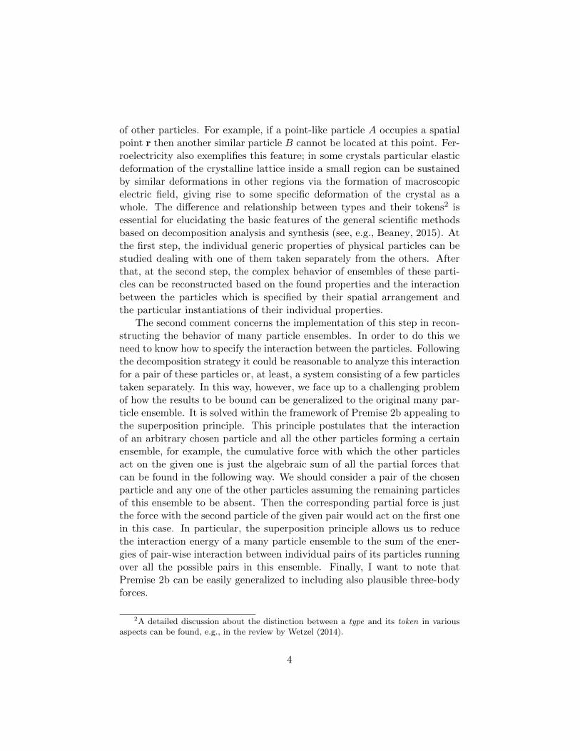
1 Principle of microlevel reducibility

Dealing with objects of the inanimate world in the frameworks of classicalphysics, we admit the existence of the microscopic (elementary) level of theirdescription. It means that in modeling such physical systems one can makeuse of the following premises to be referred further as to the principle ofmicrolevel reducibility.1

1. For any physical system there can be found a level of its microleveldescription at which the system at hand is composed of individualstructureless entities. The term ‘structureless’ is used to emphasize thefact that either these entities are really structureless or their internalstructure does not change in time during analyzed phenomena and socan be treated as a fixed characteristic of the entities.

2. All the properties exhibited by the given system can be explainedbased on or derived from

(a) the individual properties of these entities which (properties) existindependently of the presence of the other entities,

(b) the properties of pairwise interaction between entities meetingthe superposition principle.

Further these structureless entities will be called particles for short.Premise 2b may be replaced by another one using the concept of fields.

Namely, instead of a long-distance interaction of particles a certain field, forexample, electromagnetic field is introduced. This field is locally generated

1The two premises may be regarded as a particular version of reductionism, a philo-sophical concept about the relationship between complex systems as whole entities andtheir constituent parts. In actual fact the concept of reductionism is more complicatedand contradictory, for example, there are various versions of reductionism deserving anindividual consideration. Nevertheless, it should be noted that the principle of microlevelreducibility may be treated as one of the cornerstones in the research paradigm of physics,namely, it is a particular implementation of the general scientific methods based on de-composition analysis and synthesis (see, e.g., Beaney, 2015).

2

by particles, propagates in space, and, in turn, affects them. In these termsPremise 2b is read as

2. All the properties exhibited by the given system can be explainedbased on or derived from the individual properties of its constituentstructureless particles (item 2a) and

(b′) the own properties of some fields freely propagating through spaceas well as the properties of the local particle-field interactionobeying the superposition principle and being responsible for thefield generation by the particles and in turn the effects producedby these fields on the particles.

It should be noted that the concept of particle interaction based on Premise 2b′

is much reacher in properties and potentiality in describing complex systemsin comparison with that based on Premise 2b. However, if the dynamics ofa certain system is characterized by time scales much longer then the meantime during which the corresponding fields propagate in space over distancesabout the system size, Premise 2b′ is approximately reduced to Premise 2b.It will be used, for the sake of simplicity, in the following sections, althoughthe results to be obtained can be generalized to theories turning directly toPremise 2b′. Besides, strictly speaking, the use of the fields leads to thenecessity of modifying Premise 1 too because in this case a given physicalsystem is decomposed not only into structureless particles but also fieldsexisting on their own and which have to be treated as its constituent enti-ties. However various aspects of these fields regarded as individual objectson their own, i.e., beyond the scope of the interaction between the particlesthat is implemented via these fields, do not belong to the subject-matter ofthis paper.

The following two comments are also worthy of noting before passingdirectly to various consequences of the principle of microlevel reducibility.First, Premise 2a concerns the properties that are ascribed to particles indi-vidually, i.e. independently of the presence or absence of other particles. Inthis sentence by the term “properties” I actually mean a certain collectionof types of properties ascribed to the particles individually. For example,“being located at a spatial point” is a property type of point-like particlesin classical physics, it characterizes a generic feature of all these objects.“Being able to restore its previous form once the forces are no longer ap-plied” exemplifies another generic property which as a type is ascribed toall elastic springs. I noted this fact here to emphasize that particular in-stantiations of these properties, their tokens, can depend on the presence

3

of other particles. For example, if a point-like particle A occupies a spatialpoint r then another similar particle B cannot be located at this point. Fer-roelectricity also exemplifies this feature; in some crystals particular elasticdeformation of the crystalline lattice inside a small region can be sustainedby similar deformations in other regions via the formation of macroscopicelectric field, giving rise to some specific deformation of the crystal as awhole. The difference and relationship between types and their tokens2 isessential for elucidating the basic features of the general scientific methodsbased on decomposition analysis and synthesis (see, e.g., Beaney, 2015). Atthe first step, the individual generic properties of physical particles can bestudied dealing with one of them taken separately from the others. Afterthat, at the second step, the complex behavior of ensembles of these parti-cles can be reconstructed based on the found properties and the interactionbetween the particles which is specified by their spatial arrangement andthe particular instantiations of their individual properties.

The second comment concerns the implementation of this step in recon-structing the behavior of many particle ensembles. In order to do this weneed to know how to specify the interaction between the particles. Followingthe decomposition strategy it could be reasonable to analyze this interactionfor a pair of these particles or, at least, a system consisting of a few particlestaken separately. In this way, however, we face up to a challenging problemof how the results to be bound can be generalized to the original many par-ticle ensemble. It is solved within the framework of Premise 2b appealing tothe superposition principle. This principle postulates that the interactionof an arbitrary chosen particle and all the other particles forming a certainensemble, for example, the cumulative force with which the other particlesact on the given one is just the algebraic sum of all the partial forces thatcan be found in the following way. We should consider a pair of the chosenparticle and any one of the other particles assuming the remaining particlesof this ensemble to be absent. Then the corresponding partial force is justthe force with the second particle of the given pair would act on the first onein this case. In particular, the superposition principle allows us to reducethe interaction energy of a many particle ensemble to the sum of the ener-gies of pair-wise interaction between individual pairs of its particles runningover all the possible pairs in this ensemble. Finally, I want to note thatPremise 2b can be easily generalized to including also plausible three-bodyforces.

2A detailed discussion about the distinction between a type and its token in variousaspects can be found, e.g., in the review by Wetzel (2014).

4

In the next sections I present some arguments about why Newtonianmechanics is based on the mathematical formalism of second order differ-ential equations. At the first step appealing to the principle of microlevelreducibility let us try to elucidate what general mathematical form the lawsgoverning the dynamics of physical systems should have within the frame-work of classical physics.

2 Presentism and the time flow

The possibility of reducing a description of a physical system to structure-less particles and interaction between them has an important consequence.These particles cannot remember their history or foresee their future; theyjust have no means to do this, so only the present matters to them. There-fore all the plausible quantities Qα that can be used to describe the lawsgoverning the motion of a given particle α have to be taken at the currentmoment of time. Naturally there should be other characteristics of the par-ticles such as mass, charge, spin magnitude, etc. which, however, are treatedas their internal properties not changing in time. Let us regard the dynam-ics of these particles as their motion in a certain N -dimensional space RN ;for our world treated in the realm of classical physics N = 3. So the spatialposition (spatial coordinates) xα of the particle α has to enter the collectionQα. The motion of this particle is represented by the time dependencexα(t) of its position showing the points occupied previously and the pointsto be got in future according to prediction of its dynamics. However, forsuch particles

• the past no longer exists,

• the future does not exist yet,

• only the present matters to them and determines everything.

Thereby solely instantaneous characteristics of the particle motion trajec-tory xα(t) may also enter the collection Qα. They are time derivativesof xα(t) taken at the current moment of time t. In particular, it is the parti-cle velocity vα(t) = dxα(t)/dt, its acceleration aα(t) = d2xα(t)/dt2, the timederivative of third order called usually the jerk or jolt jα(t) = d3xα(t)/dt3,and so on. However, in order to construct a time derivative we have to con-sider not only the current position xα(t) of a particle but also its positionxα(t−∆) in the immediate past separated from the present by an infinitelyshort time interval ∆ → +0. Indeed, for example, the particle velocity is

5

defined as vα(t) = lim∆→+0[xα(t) − xα(t −∆)]/∆. At this place an atten-tive reader may find some contradiction, in speaking about the present weactually deal with a certain kind of instants including not only the point-like current moment of time but also other time moments belonging to someneighborhood of the current time whose size may be an infinitely small value.It causes us to speak about the thick present.

The concept of thick present is worthy of special attention because itleads directly to the formalism of differential equations and the principle ofleast action playing a crucial role in modern physics. Therefore let us focusout attention on the philosophical doctrine usually referred to as presentismwhich can be employed to penetrate deeper into the concept of thick present.

Broadly speaking, presentism is the thesis that only the present exists. Inthe given form it is a rather contradictory and ambiguous proposition beingone of the subjects of ongoing debates about the nature of time tracingtheir roots in ancient Greece. In particular, the problems of presentism aremet in the famous paradoxes of motion (see, e.g., Huggett, 2010) devisedby the Greek philosopher Zeno of Elea (circ. 490–430 BC). Unfortunately,none of Zeno’s works has survived and what we know about his paradoxescomes to us indirectly, through paraphrases of them and comments on them,primarily by Aristotle (384–322 BC), however, by Plato (428/427–348/347BC), Proclus (circ. 410–485 AD), and Simplicius (circ. 490–560 AD) savedthem for us. The names of the paradoxes were created by commentators,not by Zeno (Dowden, 2016).

We confine ourselves to the arrow paradox primarily mentioned in thecontext of the time problem. This paradox is designed to prove formallythat the flying arrow cannot move, it has to be at the rest and, so, themotion is merely an illusion. Citing Aristotle’s Physics VI,

[t]he third is . . . that the flying arrow is at rest, which result followsfrom the assumption that time is composed of moments . . . . He saysthat if everything when it occupies an equal space is at rest, and if thatwhich is in locomotion is always occupying such a space at any moment,the flying arrow is therefore motionless.

Focusing our attention on the issue in question I want to interpret the arrowparadox as three logical steps:

• time is composed of instants—point-like moments of time—and thepresent is the current moment;

• only the present matters, i.e., all the properties of the flying arrowincluding its motion at a certain velocity are determined completely

6

by its current state, i.e., the spatial point where it is currently located;

• whence it follows that the arrow motion is impossible because the stateof any arrow—flying from the left to the right, in the opposite direc-tion, or just being at the rest—is the same if at the current momentof time it is located at the same spatial point; the arrow just does not“know” in which direction it has to move.

Aristotle was the first who proposed, in his book Physics VI (Chap. 5,239b5–32), a certain solution to the arrow paradox. Since that time thisparadox having been attacked from various points of view (see, e.g., reviewsby Lepoidevin, 2002; Huggett, 2010; Dowden, 2016), a detailed analysis ofAristotle’s solution and its modern interpretation can be found in works byVlastos (1966); Lear (1981); Magidor (2008).

A naıve solution to the arrow paradox could be the proposal to includethe instantaneous velocity in the list of basic properties characterizing thecurrent arrow state. Unfortunately the instantaneous velocity, as well as therate of time changes in any quantity, cannot be attributed to an instant—a point-like moment of time. The velocity is a characteristic of a certain,maybe, infinitesimal neighborhood of this time moment (Arntzenius, 2000).For this reason Russell (1903;1937) rejects the instantaneous velocity at agiven moment to be the body’s intrinsic property having some causal power.Arguments for and against this view have been analyzed, e.g., by Arntzenius(2000); Lange (2005).

As a plausible way to overcoming this causation problem of instanta-neous velocity, a special version of presentism admits the present to havesome duration (e.g., Craig, 2000; Dainton, 2010; McKinnon, 2003). Follow-ing Hestevold (2008) it is called thick presentism. On the contrast, thinpresentism takes the present to be durationless, which, however, immedi-ately gives rise to logical puzzles like Zeno’s arrow.

In the framework of thick presentism there has been put forward a ratherpromising solution to the arrow paradox turning to the formalism of nonstan-dard analysis; for an introduction to this discipline a reader may be referredto Goldblatt (1998). Following (White, 1982; McLaughlin and Miller, 1992;McLaughlin, 1994; Arntzenius, 2000; Easwaran, 2014; Reeder, 2015) let usequip each point-like time moment t with some neighborhood of infinitesi-mal thickness 2ε, i.e., t → t = (t − ε, t + ε) and understand time events assome objects distributed inside t. Here ε is an infinitesimal—infinitely smallhyperreal number of nonstandard analysis. Below I will use the term boldinstants in order to address to such objects and not to mix them with timesintervals of finite thickness also conceded in some particular versions of thick

7

presentism. It is worthy of noting that there is no contradiction betweenthe notion of bold instants and the intuitive separability of time momentsbecause for any two moments t1 and t2 separated by arbitrary small butfinite interval the infinitesimal regions t1 and t2 do not overlap.

The notion of bold instants t opens, in particular, a gate to endowingthe instant velocity with causal power just attributing the instant velocityto the left part (t− ε, t) of t and assuming that its effect arises in the rightpart (t, t + ε) (Easwaran, 2014, a similar view was also defended by Lange(2002)). In this case, as it must, a cause and its effect are ordered in time;a cause precedes its effect.

Introducing the concept of bold instants we have to accept a specialtopological connectedness of time which is non-local on infinitesimal scales.Namely, for a time moment t at least all the previous time moments in theinfinitesimal interval (t − ε, t) are to coexist, otherwise they cannot havecausal power on it. Exactly this connectedness paves the way for propertiesthat can be attributed only to time intervals including infinitesimals to havecausal power (Lange, 2002, 2005; Harrington, 2011). Allowing the givenmultitude of time moments to exist we actually accept a special version ofthick presentism called the degree presentism proposed by Smith (2002).His account assumes that all events have past and future parts whose exis-tence degree (degree of reality) decreases to zero as their time moments goaway from the present. Baron (2015b) has developed a related account oftime called priority presentism according to which only the present entitiesexist fundamentally, whereas the past and future entities also existing aregrounded in the present.

Any version of presentism has to explain how the flow of time is im-plemented in dynamical phenomena. In the framework of thick presentismBaron (2012) puts forward the step-wise model for the flow of time consistingin temporally extended (thick) instants. Each of these instants comes intoand going our of existence in such a manner that successive thick instantspartially overlap.

At the next step in describing dynamical processes in terms of thickpresentism we face up to a problem of giving the meaning to time changesin the properties of some object for which its present partially containsits past and future parts. As a natural way to overcoming this problem,Smart (1949) introduces a complex structure of time containing in additionto the physical time a certain meta-time. Meta-time is necessary to dealwith temporal properties of events embedded into the “river of time” whenthese properties themselves change in time and a meta-time is a place wherethese changes can occur. It should be emphasized that the introduction of

8

human time

current stimuli

currentreaction

a gi

ven

indi

vidu

al

subjective component

physical timeobjective component

complex present

past of individual imaginary future

current time

bold presentcurrent time

Figure 1: Illustration of a plausible mechanism synchronizing the time flowsin the subjective and objective components of human nature.

two-dimensional time for thick presentism with bold instants does not leadto paradoxes arising in the time travel problem and used often as argumentsagainst the possibility of two-dimensional time structure. A review of thesearguments is given, e.g., by Richmond (2000); Oppy (2004); Baron (2015a).The matter is that the difference between the physical time and meta-timebecomes essential only within bold instants—the infinitesimal intervals—wherein time travels with non-zero length quantified by standard numbersare impossible.

Below I will outline my account of dynamical processes consisting inbold instants which is developed for explaining the use of differential equa-tions for modeling dynamical phenomena in classical mechanics and thevariational technique as a fundamental law governing dynamics of physicalobject. Before this, however, let me elucidate the further constructions usingthe relationship of human and physical time as a characteristic example.

As noted previously (Lubashevsky and Plawinska, 2009), two compo-nents of human nature, objective and subjective ones (Fig. 1) should bediscriminated in modeling human behavior. The objective component rep-resents the world external for a given individual and embedded in the flow ofthe physical time. The subjective component representing the internal worldof this individual is equipped with a more complex structure of time to be

9

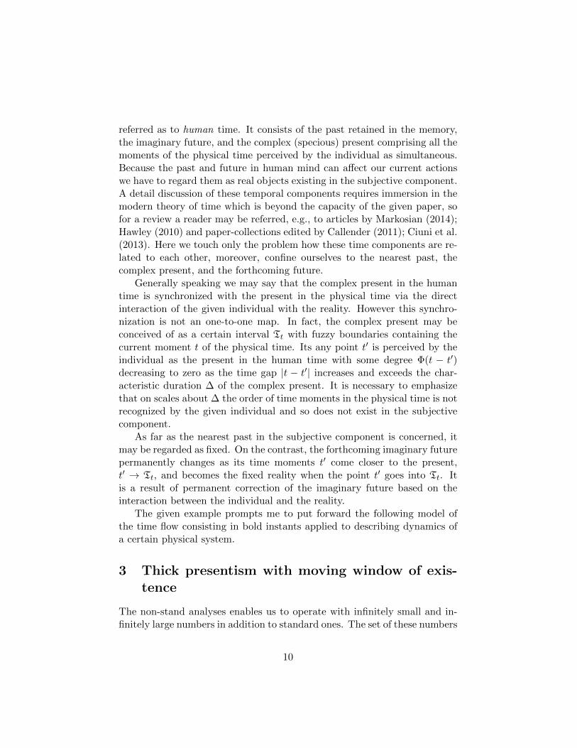
referred as to human time. It consists of the past retained in the memory,the imaginary future, and the complex (specious) present comprising all themoments of the physical time perceived by the individual as simultaneous.Because the past and future in human mind can affect our current actionswe have to regard them as real objects existing in the subjective component.A detail discussion of these temporal components requires immersion in themodern theory of time which is beyond the capacity of the given paper, sofor a review a reader may be referred, e.g., to articles by Markosian (2014);Hawley (2010) and paper-collections edited by Callender (2011); Ciuni et al.(2013). Here we touch only the problem how these time components are re-lated to each other, moreover, confine ourselves to the nearest past, thecomplex present, and the forthcoming future.

Generally speaking we may say that the complex present in the humantime is synchronized with the present in the physical time via the directinteraction of the given individual with the reality. However this synchro-nization is not an one-to-one map. In fact, the complex present may beconceived of as a certain interval Tt with fuzzy boundaries containing thecurrent moment t of the physical time. Its any point t′ is perceived by theindividual as the present in the human time with some degree Φ(t − t′)decreasing to zero as the time gap |t − t′| increases and exceeds the char-acteristic duration ∆ of the complex present. It is necessary to emphasizethat on scales about ∆ the order of time moments in the physical time is notrecognized by the given individual and so does not exist in the subjectivecomponent.

As far as the nearest past in the subjective component is concerned, itmay be regarded as fixed. On the contrast, the forthcoming imaginary futurepermanently changes as its time moments t′ come closer to the present,t′ → Tt, and becomes the fixed reality when the point t′ goes into Tt. Itis a result of permanent correction of the imaginary future based on theinteraction between the individual and the reality.

The given example prompts me to put forward the following model ofthe time flow consisting in bold instants applied to describing dynamics ofa certain physical system.

3 Thick presentism with moving window of exis-tence

The non-stand analyses enables us to operate with infinitely small and in-finitely large numbers in addition to standard ones. The set of these numbers

10

degree of existence

meta-time

physical time

physical

time, t

meta-time, T moving windowof existence

position inspace, x

forward

causation backward

causation

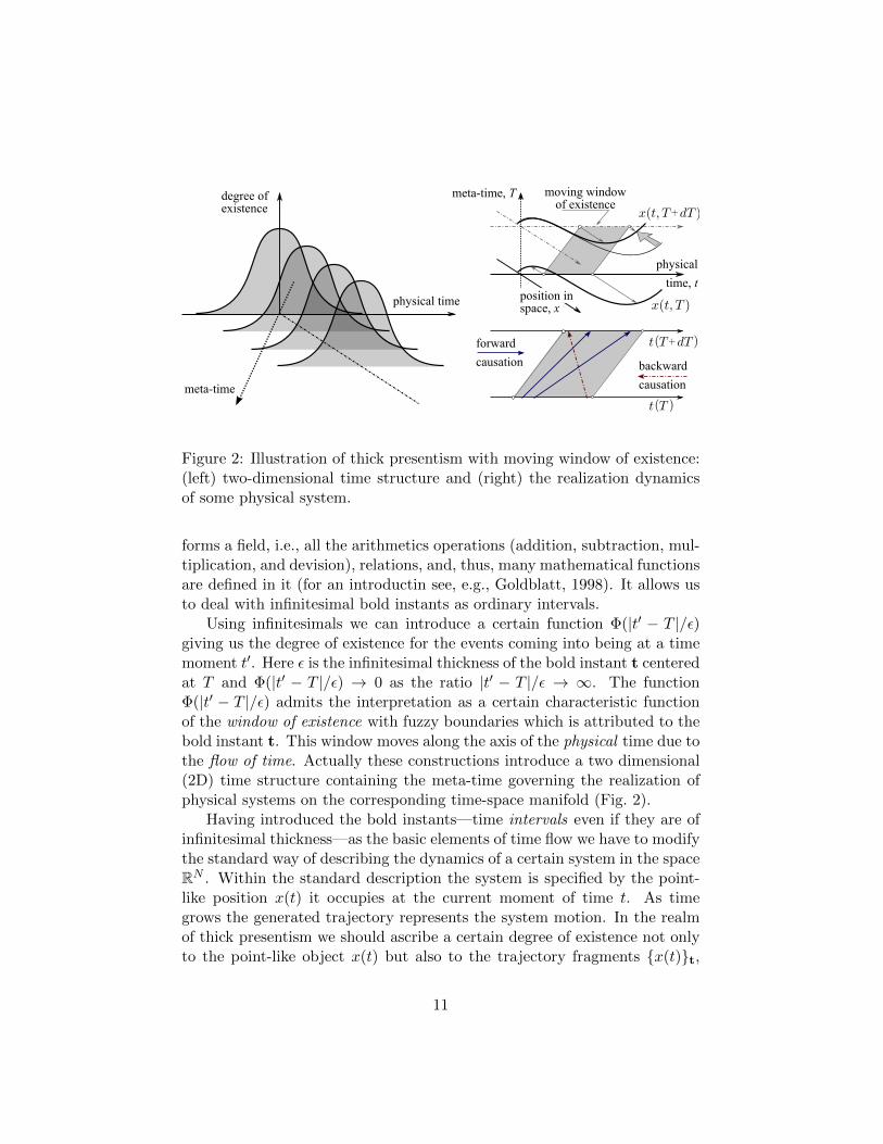
Figure 2: Illustration of thick presentism with moving window of existence:(left) two-dimensional time structure and (right) the realization dynamicsof some physical system.

forms a field, i.e., all the arithmetics operations (addition, subtraction, mul-tiplication, and devision), relations, and, thus, many mathematical functionsare defined in it (for an introductin see, e.g., Goldblatt, 1998). It allows usto deal with infinitesimal bold instants as ordinary intervals.

Using infinitesimals we can introduce a certain function Φ(|t′ − T |/ε)giving us the degree of existence for the events coming into being at a timemoment t′. Here ε is the infinitesimal thickness of the bold instant t centeredat T and Φ(|t′ − T |/ε) → 0 as the ratio |t′ − T |/ε → ∞. The functionΦ(|t′ − T |/ε) admits the interpretation as a certain characteristic functionof the window of existence with fuzzy boundaries which is attributed to thebold instant t. This window moves along the axis of the physical time due tothe flow of time. Actually these constructions introduce a two dimensional(2D) time structure containing the meta-time governing the realization ofphysical systems on the corresponding time-space manifold (Fig. 2).

Having introduced the bold instants—time intervals even if they are ofinfinitesimal thickness—as the basic elements of time flow we have to modifythe standard way of describing the dynamics of a certain system in the spaceRN . Within the standard description the system is specified by the point-like position x(t) it occupies at the current moment of time t. As timegrows the generated trajectory represents the system motion. In the realmof thick presentism we should ascribe a certain degree of existence not onlyto the point-like object x(t) but also to the trajectory fragments x(t)t,

11

where t ∈ t. It means that the very basic level of the system descriptionmust consist in the trajectories, at least, their parts rather than point-likeobjects and causal power may be attributed only to these basic elements.We should to do this at each moment T of meta-time, otherwise, evolutionand emergence as dynamical phenomena are merely a mirage—everything isfixed beforehand. In other words, the basic element of the system descriptionin the 2D-time structure is given by the trajectory x(t, T ) or, speakingmore strictly, its partition specified by bold instants t. I have used the termtrajectory to emphasize that these basic elements are certain functions ofthe argument t running from −∞ to +∞ rather than points of the spaceRN ; here the meta-time T plays the role of a parameter.

In these terms the system dynamics at any moment T of meta-time ischaracterized by the following components:

• the past of the system: x(t, T ) matching t < T and t /∈ tT ,

• the thick present of the system: x(t, T ) where t ∈ tT ,

• the future of the system: x(t, T ) matching t > T and t /∈ tT

depending on T . It is worthy of noting that involving the past and furtherinto consideration of causal processes affecting the system dynamics doesnot contradict the previous statement about their absence for structurelessparticles of classical physics. Such particles have no means to rememberindividually their past or to predict their future. However in the case underconsideration the causal power of the past and future is due to the physicalproperties of the time flow itself rather than that of the particles and spendsover temporal intervals of infinitesimal thickness only.

In the framework of thick presentism all the properties of the given sys-tem at the current moment T of meta-time must be determined completelyby the trajectory x(t, T ), whereas the presence of its points in the reality isdetermined by the current position of the window of existence. It concernsalso the property I call the sensitivity of the given system to the flow ofmeta-time or simply meta-time sensitivity. It quantifies the variation of thetrajectory x(t, T ) caused by the meta-time flow provided the correspond-ing part of the trajectory is present in the reality. The partial existence ofa trajectory fragment in the reality decreases its variation so the governingequation for these trajectory variations can be written as

∂x(t, T )

∂T= P

(|t− T |ε

)Ω [x(t, T )] , (1)

12

4 2 0 2 4time difference t, in ε

0.1

0.0

0.1

0.2

0.3

0.4

0.5

time

kern

el K

i(t)

, in ε−

(i+

1)

i=0

4 2 0 2 4time difference t, in ε

0.3

0.2

0.1

0.0

0.1

0.2

0.3

i=1

4 2 0 2 4time difference t, in ε

0.4

0.3

0.2

0.1

0.0

0.1

0.2

i=2

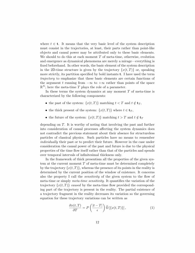
Figure 3: Typical forms of kernels determining nonlocal contribution ofdifferent time moments to the system meta-time sensitivity.

where the operator Ω [x(t, T )] specifies the meta-time sensitivity of thegiven system with the trajectory x(t, T ). Figure 2 (right fragment) illus-trates the variations of the system trajectory as the meta-time grows. Itshould be noted that within the bold instant tT the time moments may notbe ordered in their effects, i.e., the variation of the system trajectory atmoment t ∈ tT can be partially caused by time moments preceding as wellas succeeding it. In the latter case we can speak about backward causation(for a general discussion on the backward causation problem a reader maybe referred to Faye, 2010).

Equation (1) can relate to one another only the trajectory fragmentscorresponding to bold instants t that either contain the time moment T orare distant from it over scales about ε. So terms similar to

+∞∫−∞

dt′Ki

(t− t′

ε

)x(t′, T ) (2)

should mainly contribute to the variation of the trajectory x(t, T ) at thepoint t ∈ tT and the typical forms of the kernels Ki (. . .) are exemplified inFig. 3. Such nonlocal effects can connect only time moments separated byinfinitely small time lags whereas the motion trajectory of systems at handare to be smooth curves. In this case the nonlocal operator Ω [x(t, T )]should reduce to a certain local function ω whose arguments are the currentsystem position x and its various derivatives taken at the current moment t

Ω [x(t, T )] =⇒ ω

[x(t, T ),

∂x(t, T )

∂t,∂2x(t, T )

∂t2,∂3x(t, T )

∂t3, . . .

]. (3)

13

physical

time, t

posi

tion

in s

pace

, x

current bold instant

emerged past

"initial" future

Figure 4: Emergence ofthe system past match-ing the system dynam-ics governed by stablelaws which are deter-mined completely by thesystem physics.

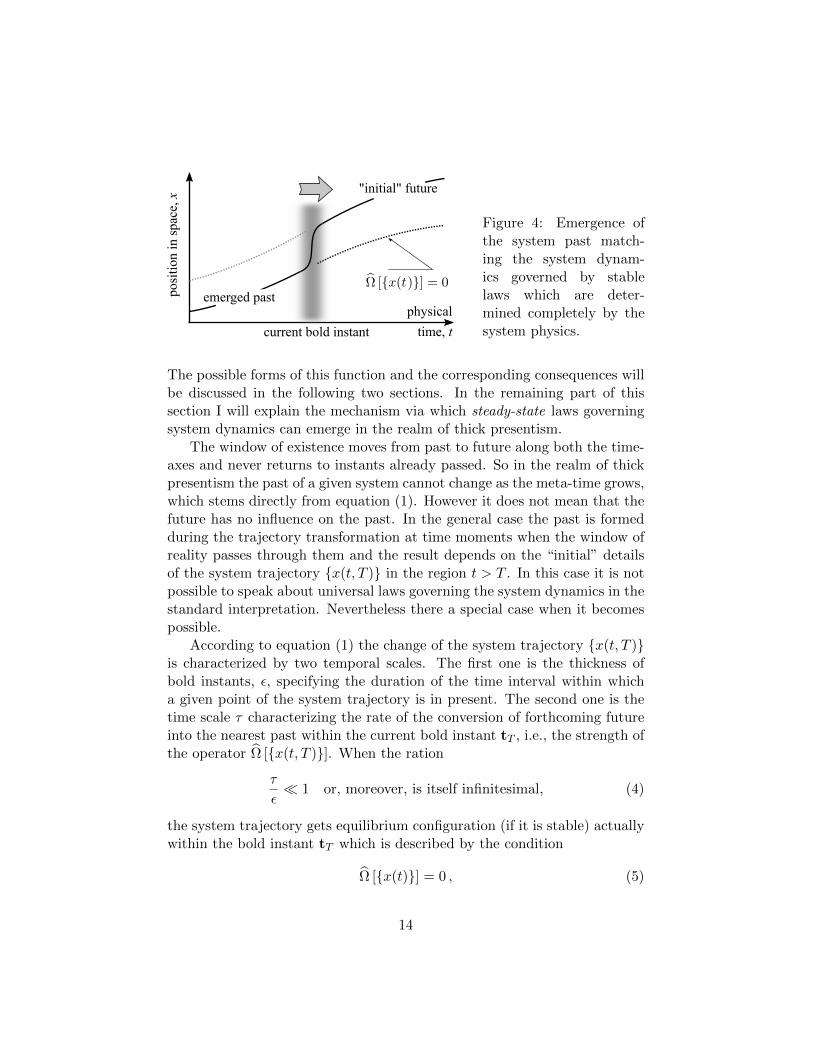
The possible forms of this function and the corresponding consequences willbe discussed in the following two sections. In the remaining part of thissection I will explain the mechanism via which steady-state laws governingsystem dynamics can emerge in the realm of thick presentism.

The window of existence moves from past to future along both the time-axes and never returns to instants already passed. So in the realm of thickpresentism the past of a given system cannot change as the meta-time grows,which stems directly from equation (1). However it does not mean that thefuture has no influence on the past. In the general case the past is formedduring the trajectory transformation at time moments when the window ofreality passes through them and the result depends on the “initial” detailsof the system trajectory x(t, T ) in the region t > T . In this case it is notpossible to speak about universal laws governing the system dynamics in thestandard interpretation. Nevertheless there a special case when it becomespossible.

According to equation (1) the change of the system trajectory x(t, T )is characterized by two temporal scales. The first one is the thickness ofbold instants, ε, specifying the duration of the time interval within whicha given point of the system trajectory is in present. The second one is thetime scale τ characterizing the rate of the conversion of forthcoming futureinto the nearest past within the current bold instant tT , i.e., the strength ofthe operator Ω [x(t, T )]. When the ration

τ

ε 1 or, moreover, is itself infinitesimal, (4)

the system trajectory gets equilibrium configuration (if it is stable) actuallywithin the bold instant tT which is described by the condition

Ω [x(t)] = 0 , (5)

14

where the steady-state trajectory x(t) does not depend on meta-time T .In this case the system past is mainly determined by equality (5) and

“forgets” completely the “initial” future of the system. As a result the lawsdescribing the newly emerged past as the present may be of a universalform reflecting only the physics of a given system. Figure 4 illustrates thissituation.

4 Steady-state laws of system dynamics

I will call condition (4) the limit of steady-state laws and will assume it tohold in our reality. In this case the system dynamics described in terms ofthe position x(t) in the space RN occupied by the system in the immediatepast obeys the equation

ω

[x(t),

dx(t)

dt,d2x(t)

dt2,d3x(t)

dt3, . . .

]= 0 (6)

by virtue of (3).Expression (6) is the key point determining further constructions in the

present paper. In particular, it explains why the laws governing the dynam-ics of systems in the framework of classical physics admits a representationin the form of some formulas joining together the time derivatives of themotion trajectory taken at the current moment of time. Thereby the for-malism of differential equations is actually the native language of physicsor, speaking more strictly, Newtonian mechanics. Naturally the question onwhether differential equations are the very basic formalism of physics hasbeen in the focus of long-term debates and attacked from various points ofview, for a short review see, e.g., Stoltzner (2006) and references therein.

Causal relations can be also attributed to law (6), at least, when thelist of arguments of the function ω(. . .) is finite. In this case resolving equa-tion (6) with respect to the highest order m time derivative of x(t) we obtainthe expression

dmx

dtm= Φ

(x,dx

dt,d2x

dt2, . . . ,

dm−1x

dtm−1

)(7)

which admits interpretation as a causal relationship between the lower ordertime derivatives

x,dx

dt,d2x

dt2, . . . ,

dm−1x

dtm−1(8)

playing the role of causes and the highest time derivative dmx/dtm beingtheir effect. Indeed, when the system trajectory undergoes sharp variations

15

inside the bold instant tT the highest derivative demonstrates changes mostdrastically and it is possible to say that the collection of quantities (8) finallycause the highest derivative to take value (7).

The accepted hypothesis on the finite number of arguments in the func-tion ω(. . .) can be directly justified if the field of hyperreal numbers is ex-tended to a ring including nilpotent infinitesimals. Nilpotents are nonzeroinfinitely small numbers that yield zero when being multiplied by themselvesfor a certain number of times. So if the kernels Ki(. . .) contain nilpotentcofactors, the meta-time sensitivity operator Ω[x(t, T )] can comprise onlyfinite order power terms with respect to quantities similar to (2). In a sim-ilar way Reeder (2015) uses nilpotents for constructing a novel solution toZeno’s arrow.

5 Variational formulation of steady-state dynam-ics

There is a special case worthy of individual attention that admits the intro-duction of a certain functional

L[x(t, T )]

to be call action following the traditions accepted in physics. This functionalspecifies the operator of meta-time sensitivity as its functional derivative

Ω[x(t, T )] = −δS[x(t, T )]δx(t, T )

. (9)

Because bold instants can couple only infinitely close time moments theaction functional in the general form can be written as

L[x(t, T )] =

+∞∫−∞

dtL

[x(t, T ),

∂x(t, T )

∂t,∂2x(t, T )

∂t2,∂3x(t, T )

∂t3, . . .

], (10)

where function

L

[x(t, T ),

∂x(t, T )

∂t,∂2x(t, T )

∂t2,∂3x(t, T )

∂t3, . . .

](11)

is called the Lagrangian of a given system.In the limit of stead-state laws the trajectory x(t) meeting condi-

tion (5) should be stable with respect to small (infinitesimal) variations

x(t, T ) = x(t) + δx(t, T ) .

16

It means that the variations δx(t, T ) have to fade as meta-time T grows. Thisstability condition directly gives rise to the following requirement which hasto be imposed on the corresponding form of the action functional and itsLagrangian.

Principle of Least Actions: Let a physical system admit the introduction of theaction functional (10) describing its dynamics in meta-time. Then its steady-statetrajectory x(t) describing the system motion in the past including the immedi-ate past matches the minimal value of the action functional among all the otherpossible trajectories

x(t) =⇒ min

+∞∫−∞

dtL

[x(t),

dx(t)

dt,d2x(t)

dt2,d3x(t)

dt3, . . .

]. (12)

Actually this principle is in one-to-one correspondence with the principleof least actions well-known in physics provided the Lagrangian L(x, dx/dt)depends only on the system position x and the velocity dx/dt.

6 Notion of phase space

In the previous sections we have considered the general description of systemdynamics in the framework of thick presentism and the limit of steady-statelaws has been assumed to hold in our world. In this case the dynamics of aphysical system conceived of as the motion of a point x in a certain spaceis governed by equation (6) joining together all the time derivatives of thetrajectory x(t) taken at the current moment of time t.

In what follows, first, we will confine ourselves to the case where thenumber of the time derivatives entering the right-hand side of (6) is finitefor any physical object. Second, we will consider an ensemble of structurelessparticles whose individual motion can be represented as the motion of a pointxα in the space RN ; in our world N = 3. This ensemble may be described asa point x = xα of the space RNM , where M is the number of particles inthe given ensemble. Besides, for the sake of simplicity we will assume thatfor all the particles only the first (m− 1) derivatives of their coordinates xαenter equation (6).3

3The further constructions can be easily generalized to the case when the state of differ-ent particles is characterized by different parameters mα, which, however, over-complicatesthe mathematical expressions without any reason required for understanding the subject.

17

Under these conditions equation (6) treated as some equality can be re-served with respect to the highest derivative dmx/dtm which gives us expres-sion (7). This expression may be interpreted as a causal type relationshipbetween the time derivatives of order less than m (including the zero-th or-der derivative just being the particle positions) and the derivative dmx/dtm.For individual particles formula (7) takes the form

dmxαdtm

= Φα

(x,dx

dt,d2x

dt2, . . . ,

dm−1x

dtm−1

), (13)

where the particle index α is omitted at the list of arguments in the right-hand side of (13), which denotes that all the particles of a given ensembleshould be counted here because of the particle interaction.

The fact that the right-hand side of equation (13) contains only thetime derivatives of order less than m does not mean the mutual indepen-dence of these quantities. There could be conceived of some additional con-strains imposed on this system such that one of these derivatives, mainly,dm−1x/dtm−1 is completely determined by the others. It actually reducesthe number of arguments in (13). Therefore below we may assume thecollection of quantities

Qα =

x,dx

dt,d2x

dt2, . . . ,

dm−1x

dtm−1

α

, (14)

to be mutually independent for all the particles α. It means that forarbitrary chosen values there can be found an instantiation of this systemsuch that during its motion these time derivatives take the given values ata given moment of time t.

Now we can introduce the notion of the phase space

P =

x,dx

dt,d2x

dt2, . . . ,

dm−1x

dtm−1

(15)

for the system at hand regarded as a whole. If we know the position of thesystem in the space P treated as a point θ with the coordinates

θ =

(x,dx

dt,d2x

dt2, . . . ,

dm−1x

dtm−1

), (16)

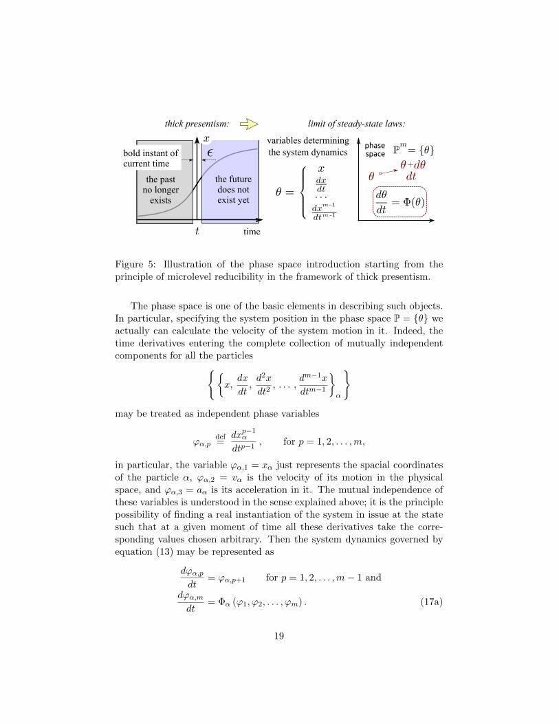
then the rate of the system motion in the phase space P is completely de-termined via relationship (13). Solving this equation we can construct thetrajectory of the system motion. The aforesaid is illustrated in Fig. 5.

18

the future does not exist yet

phasespace

time

variables determiningthe system dynamics

the past no longer

exists

thick presentism: limit of steady-state laws:

bold instant of current time

Figure 5: Illustration of the phase space introduction starting from theprinciple of microlevel reducibility in the framework of thick presentism.

The phase space is one of the basic elements in describing such objects.In particular, specifying the system position in the phase space P = θ weactually can calculate the velocity of the system motion in it. Indeed, thetime derivatives entering the complete collection of mutually independentcomponents for all the particles

x,dx

dt,d2x

dt2, . . . ,

dm−1x

dtm−1

α

may be treated as independent phase variables

ϕα,pdef=

dxp−1α

dtp−1, for p = 1, 2, . . . ,m,

in particular, the variable ϕα,1 = xα just represents the spacial coordinatesof the particle α, ϕα,2 = vα is the velocity of its motion in the physicalspace, and ϕα,3 = aα is its acceleration in it. The mutual independence ofthese variables is understood in the sense explained above; it is the principlepossibility of finding a real instantiation of the system in issue at the statesuch that at a given moment of time all these derivatives take the corre-sponding values chosen arbitrary. Then the system dynamics governed byequation (13) may be represented as

dϕα,pdt

= ϕα,p+1 for p = 1, 2, . . . ,m− 1 and

dϕα,mdt

= Φα (ϕ1, ϕ2, . . . , ϕm) . (17a)

19

Here, as previously, omitting the index α at the arguments of the functionΦα. . . denotes that its list of arguments should contain the phase variablesϕα,p of all the particles. These differential equations which symbolicallymay be written as

dθ

dt= Φ(θ) (17b)

determine all the laws of the system dynamics.The existence of equations (17) endows the inanimate world in the realm

of classic physic with a fundamental property described by two notions re-flecting its different aspects. One of them is the notion of initial conditions.4

Namely, if we know the system position θ0 in the phase space P at an ar-bitrary chosen moment of time t0 then, generally speaking, equations (17)possess the unique solution for t > t0

θ = θ(t, θ0) such that at t = t0 θ(t0, θ0) = θ0 . (18)

In other words, if the “forces” Φ(θ) and the initial system position θ0 areknown, then the system dynamics can be calculated, at least, in principle.It means that inanimate systems have no memory; if we know what is goingon with such a system at a given moment of time, then its “history” doesnot matter, which was claimed previously appealing to Premise 1.

The other one is the notion of the determinism of physical systems; ifwe repeat the system motion under the same conditions with respect to theinitial position θ0 and the “forces” Φ(θ) acting on the system, then the sametrajectory of system motion will be reproduced. Drawing this conclusion weactually have assumed implicitly that the “forces” Φ(θ) do not depend onthe time t. If it is not so, then we can expand the system to include externalobjects causing the time dependence of these “forces.” The feasibility ofsuch an extension is justified by the principle of microlevel reducibility. Infact it claims that at the microslevel describing completely a given systemthere are only structureless constituent particles and the interaction betweenthem. So there no factors that can cause the time dependence of the “forces”Φ(θ) and, in particular, endow them with random properties.

Brief digression: It should be noted that this determinism does not exclude highlycomplex dynamics of nonlinear physical systems manifesting itself in phenomenausually referred to as dynamical chaos. Dynamical chaos can be observed when themotion of a system in its phase space is confined to a certain bounded domain andthe motion trajectories are unstable with respect to small perturbations. This insta-bility means that two trajectories of such a system initially going in close proximity4Actually the range of applicability of notion of initial conditions is much wider than

Newtonian mechanics, which however is beyond the scope of our discussion.

20

to each other diverge substantially as time goes on, and, finally, the initial proximityof the two trajectories becomes unrecognizable. These effects make the dynamics ofsuch systems practically unpredictable. For example, in numerical solution of equa-tions (17) the discretization of continuous functions and round-off errors play the roleof disturbing factors responsible for a significant dependence of the found solutionson the selected time step in discretization and particular details of arithmetic oper-ations at a used computer. In studying systems with dynamical chaos in laboratoryexperiments the presence of weak uncontrollable factors is also inevitable. Moreover,there is a reason arguing for the fact that the notion of dynamical chaos is a funda-mental problem rather than a particular question about practical implementations ofsystem dynamics. The determinism of physical systems implies the reproducibilityof their motion trajectories provided the same initial conditions are reproduced eachtime. However, in trying to control extremely small variations in the system phasevariables we can face up to effects lying beyond the range of applicability of classicalphysic. So in studding various instantiations of one system it can be necessary toassume that each time the initial conditions are not set equal but distributed randomlyinside a certain, maybe, very small domain. So determinism and dynamical chaosare not contradictory but complementary concepts reflecting different aspects of thedynamics of physical systems in the realm of classical physics.

7 Energy conservation and Newton’s second law

Appealing to the concepts of thick presentism it is not possible to find outthe order m − 1 of the derivative dm−1x/dtm−1 that determines how manycomponents collection (14) contains, i.e. to specify the structure of the phasespace P (15). From physics we know that m = 2, i.e., for any ensemble ofclassical particles the phase space consists of the spatial coordinates andvelocities of the particles making up it. Let us try to elucidate whether thistype phase space endows the corresponding systems with unique propertiesvia which such systems stand out against the other objects.

In the simplest case, i.e., when the value m = 1, the phase space con-tains only the spatial positions of particles P1 = x. In this instance therespective systems tend to go directly to spacial “stationary” points xeq suchthat

dxαdt

= Φα,1 (xeq) = 0 for all α,

if, naturally, they are stable. This class of models, broadly speaking, isthe heart of Aristotelian physics assuming, in particular, that for a bodyto move some force should act on it. There are many examples of realphysical objects exhibiting complex behaviour that are effectively describedusing the notions inherited from Aristotelian physic. The complexity of

21

their dynamics is due to the fact that all their stationary points turn out tobe unstable and, instead, some complex attractors, i.e., multitudes towardwhich systems tend to evolve, arise in the phase space P1. Nevertheless, ifour inanimate world were governed solely by Aristotelian physics it wouldbe rather poor in properties. For example, if the motion of planets of a solarsystem obeyed such laws then they would drop to its sun and the galaxiescould not form.

The next case with respect to the simplicity of phase spaces matchesm = 2. It is our world; the phase space of physical particles, at least, withinNewtonian mechanics consists of their spatial coordinates and velocities,

P2 =

x, v =

dx

dt

, (19)

which together determine the next order time derivative, the particle accel-eration,

aα =d2xαdt2

= Φα,2 (x, v) . (20)

In other words, in Newtonian physics for a body to accelerate some forcesshould act on it, whereas in Aristotelian physics for a body to move someforces should act on it. The systems whose dynamics is described by thephase space P2 possess two distinctive features.

One of them, usually called the dynamics reversibility, is exhibited bysystems where the regular “force” Φα,2 (x) depends only on the particlepositions x. In this case the governing equation (20) is symmetrical withrespect to changing the time flow direction, i.e. the replacement t → −t.This symmetry is responsible for the fact that if at the end of motion thevelocities of all the particles are inverted, vα → −vα, then they should moveback along the same trajectories.

The other one is the possibility of introducing the notion of energy forthe real physical systems. At the microlevel the energy, comprising thecomponents of the kinetic and potential energy, is a certain function

H(x, v) (21)

whose value does not change during the system motion. Namely, if x(t) is atrajectory of system motion then the formal function on t

H(t)def= H

[x(t), v(t) =

dx(t)

dt

](22)

in fact does not depend on the time t. Such systems are called conserva-tive. The existence of the energy H(x, v) does not necessary stem from the

22

governing equation (20) but is actually an additional assumption about thebasic properties of physical systems at the microlevel. Naturally, it imposessome conditions on the possible forms of the function Φα,2(x, v).

The two features endow physical systems with rich properties and com-plex behavior. For example, although in a solar system the planets areattracted by the sun, they do not drop on it because when a planet comescloser to the sun its kinetic energy grows, preventing the direct fall on thesun. Naturally, this planet should not move initially along a straight linepassing exactly through the sun. The reversibility is responsible for thisplanet to tend to return to the initial state or its analogy after passing thepoint at the planet trajectory located at the shortest distance to the sun.Broadly speaking, the existence of energy endows physical objects with acertain analogy of memory. Certainly, if the initial conditions for a givensystem are known, its further dynamics is determined completely, at least,in principle, so the previous system history does not matter. Nevertheless,the conservative systems “do not forget” their initial states in the meaningthat the motion trajectories matching different values of the energy cannotbe mixed.5

Summarizing this discussion about the systems with the phase spaceP2 we may claim that it is the simplest situation when the correspondingphysical world is reach in properties.

As far as systems with a phase space containing time derivatives of higherorders are concerned, they seem not to admit the introduction of the energyat all in a self-consistent way. In order to explain this fact we reproduce theconstruction of the governing equations for such systems of particles usingLagrangian formulation of Newtonian mechanics based on the principle ofleast actions. It is worthy of noting that in some sense Lagrangian formu-lation of mechanics is more general than its formulation directly appealingto Newton’s laws. Indeed in the latter case the existence of energy is anadditional assumption imposing certain conditions on the forces with whichphysical particles interact with one another. In Lagrangian formulation the

5First, it should be noted that a many-particle ensemble can exhibit so complex dy-namics that it could be impossible to track its motion from a given initial state withinphysically achievable accuracy. In this case it possible to speak about the effective for-getting of the initial conditions. The latter also concerns extremely weak perturbations.Second, there are systems with highly complex dynamics whose description does not ad-mit any energy conservation and their motion is irreversible; the term dynamical chaosnoted before is usually used to refer to these phenomena. Nevertheless it does not con-tradict to the present argumentation because the corresponding irreversible descriptionis obtained via the reduction of equation (20) and assuming the presence of a certainexternal environment weakly interacting with a system at hand.

23

existence of some function, the Lagrangian L, reduced then to the systemenergy is the pivot point and the derived equation governing the systemdynamics originally contain the forces meeting the required conditions.

As the general case, let us consider a system with the phase space

Pm = θm =

x,dx

dt,d2x

dt2, . . . ,

dm−1x

dtm−1

,

where m is a certain number not necessary equal to 2. The pivot pointof Lagrangian formalism is the introduction of a certain functional Lx(t)determined for any arbitrary trajectory x(t)t=tet=ts starting and ending atsome time moments t = ts and t = te, respectively. The notion of functionalmeans that for any given trajectory x(t) we can calculate a certain numberLx(t) which is treated as a measure of its “quality” in the realm of theLagrangian mechanics. Since the systems at hand do not possess memoryand cannot predict their future, all their significant characteristics includingthe “quality” of motion have to be determined by the local properties ofthe trajectory x(t). In the given case, it is the collection θn of the phasevariables x, dx/dt, . . . , dm−1x/dtm−1. Therefore the functional Lx(t) hasto be of the integral form

Lx(t) =

te∫ts

L

(x,dx

dt,d2x

dt2, . . . ,

dm−1x

dtm−1

)dt , (23)

where L(. . .) is some function of these n phase variables. The principleof least actions implies that “the Nature chooses the best trajectories toimplement” the dynamics of mechanical systems. In other words, a realtrajectory of system motion matches the minimum of functional (23) (orits maximum within the replacement L → −L) with respect to all possiblevariations near this real trajectory (Fig. 6).

It is worthy of noting that in spite of its long-term history the funda-mentality of the principle of least actions is up to now a challenging problemand there are a number of arguments for and against it from various pointsof view. Their brief review can be found, e.g., in Stoltzner (2006) as well asa detailed analysis of its ontological roots has be given by Stoltzner (2003,2009); Katzav (2004); Smart and Thebault (2015); Terekhovich (2015). Nev-ertheless its high efficient in many different branches of physics strongly ar-gues for its real fundamentality. In Section 5 I have demonstrated that thisprinciple can be derived based on the concepts of thick presentism for sys-tems whose phase space contains hight order time derivatives as individualphase variables.

24

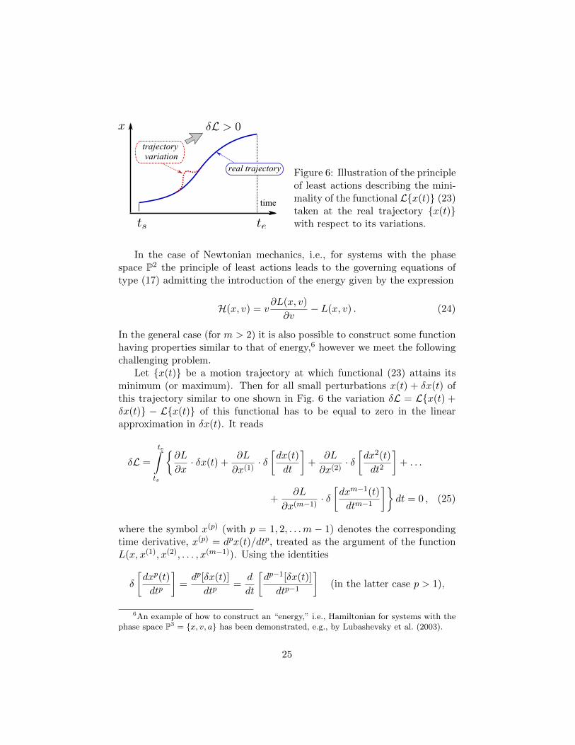
Figure 6: Illustration of the principleof least actions describing the mini-mality of the functional Lx(t) (23)taken at the real trajectory x(t)with respect to its variations.

In the case of Newtonian mechanics, i.e., for systems with the phasespace P2 the principle of least actions leads to the governing equations oftype (17) admitting the introduction of the energy given by the expression

H(x, v) = v∂L(x, v)

∂v− L(x, v) . (24)

In the general case (for m > 2) it is also possible to construct some functionhaving properties similar to that of energy,6 however we meet the followingchallenging problem.

Let x(t) be a motion trajectory at which functional (23) attains itsminimum (or maximum). Then for all small perturbations x(t) + δx(t) ofthis trajectory similar to one shown in Fig. 6 the variation δL = Lx(t) +δx(t) − Lx(t) of this functional has to be equal to zero in the linearapproximation in δx(t). It reads

δL =

te∫ts

∂L

∂x· δx(t) +

∂L

∂x(1)· δ[dx(t)

dt

]+

∂L

∂x(2)· δ[dx2(t)

dt2

]+ . . .

+∂L

∂x(m−1)· δ[dxm−1(t)

dtm−1

]dt = 0 , (25)

where the symbol x(p) (with p = 1, 2, . . .m − 1) denotes the correspondingtime derivative, x(p) = dpx(t)/dtp, treated as the argument of the functionL(x, x(1), x(2), . . . , x(m−1)). Using the identities

δ

[dxp(t)

dtp

]=dp[δx(t)]

dtp=

d

dt

[dp−1[δx(t)]

dtp−1

](in the latter case p > 1),

6An example of how to construct an “energy,” i.e., Hamiltonian for systems with thephase space P3 = x, v, a has been demonstrated, e.g., by Lubashevsky et al. (2003).

25

the rule of integration by parts

te∫ts

U(t)dV (t)

dtdt =

[U(t)V (t)

]t=tet=ts−

te∫ts

V (t)dU(t)

dtdt ,

and choosing the trajectory perturbations δx(t) such that (it is our right)

δx(t)|t=ts,tp = 0 ,dp[δx(t)]

dtp

∣∣∣∣t=ts,tp

= 0 (for p = 1, 2, . . . ,m− 1)

equality (25) is reduced to

δL =

te∫ts

∂L

∂x− d

dt

∂L

∂x(1)+

(d

dt

)2 ∂L

∂x(2)− . . .

+ (−1)m−1

(d

dt

)m−1 ∂L

∂x(m−1)

δx(t) dt = 0 . (26)

Because equality (26) must hold for any particular perturbation of the tra-jectory x(t) this trajectory has to obey the equation

∂L

∂x− d

dt

∂L

∂x(1)+

(d

dt

)2 ∂L

∂x(2)− . . .+(−1)m−1

(d

dt

)m−1 ∂L

∂x(m−1)= 0 . (27)

The time derivative of the highest order contained in equation (27) is

d2(m−1)x/dt2(m−1) ;

it enters this equation via the last term as the item

(−1)m−1 ∂2L

∂[x(m−1)]2· d

2(m−1)x

dt2(m−1).

When the derivative ∂2L/∂[x(m−1)]2 is not equal to zero,7 i.e., the Lagran-gian L(. . .) is not a linear function with respect to its argument dm−1x/dtm−1,equation (27) can be directly resolved with respect to the derivative

d2(m−1)x

dt2(m−1)

7In the case of Newtonian mechanics with the phase space P2 the corresponding termis just the mass m of a given particle, ∂2L/∂[x(2)]2 = m.

26

and rewritten as

d2(m−1)x

dt2(m−1)= Φ∗

(x,dx

dt,d2x

dt2, . . . ,

d2m−3x

dt2m−3

), (28)

where Φ∗(. . .) is a certain function. Equation (28) governs the dynamics ofthe system in issue and can be regarded as its basic law written in the formof differential equation.8

When the number of the phase variables forming the phase space Pm islarger than two, m > 2, the obtained governing equation (28) comes in con-flict with the initial assumption about the properties of the given physicalsystem. The matter is that the number of the arguments of the functionΦ∗(. . .) exceeds the dimension of the phase space Pm because 2(m− 1) > mfor m > 2. Thereby we cannot treat equation (28) as a law governing the de-terministic motion of a certain dynamical system in the phase space Pm. In-deed, to do this we need that the point θm = x, dx/dt, . . . , dm−1x/dtm−1of the phase space Pm determine completely the rate of the system motionin it, in other words, the corresponding governing equation should be ofform dθm/dt = Φ(θm) (see equation (17)). However, the obtained equa-tion (28) stemming from the principle of least actions contradicts this re-quirement because its right hand side contains the time derivatives higherthan d(m−1)x/dt(m−1) for m > 2. Therefore in order to construct a solu-tion of equation (28) dealing with only the phase space Pm we need someadditional information about, for example, the terminal point of the ana-lyzed trajectory. The latter feature, however, contradicts the principle ofmicrolevel reducibility because according this principle the current state ofsuch a system should determine its further motion completely.

Summarizing this discussion we see that only in the case of m = 2equation (28) following from the principle of least actions for trajectories inthe phase space Pm admits the interpretation in terms of a certain dynamicalsystem whose motion is completely specified within this phase space. Ifm = 1 the minimality of functional (23) does not describe any dynamics.Therefore, it is likely that the notion of the energy H(x, v) can be introduced

8Lagrangian mechanics with higher order time derivatives is well known and was de-veloped during the middle of the XIX century by Ostrogradski (1850). So here I havepresented the results in a rather symbolic form emphasizing the features essential for ourconsideration. Mechanics dealing with equation (28) with m > 2 as one describing someinitial value problem faces up to the Ostrogradsky instability (see, e.g., Woodard, 2007;Stephen, 2008; Smilga, 2009), which can be used for explaining why no differential equa-tions of higher order than two appear to describe physical phenomena (Motohashi andSuyama, 2015). There are also arguments for the latter conclusion appealing to meta-physical aspects of time changes in physical quantities (Easwaran, 2014).

27

in a self-consistent way only for systems with the phase space P2 = x, vwhere the governing laws can be written as differential equations of thesecond order.

8 Conclusion

In the given paper I have presented arguments for the relationship betweenthe notions and formalism used in the basic laws of classical physics andthe existence of the microlevel of description of the corresponding physicalsystems which obeys the principle of microlevel reducibility.

According to this principle, first, any system belonging to the realm ofclassical physics admits the representation as an ensemble of structurelessparticles with certain properties ascribed to them individually. Second, theinteraction between these particles is supposed to be determined completelyby their individual properties and to meet the superposition principle. In thegiven case the superposition principle is reduced either to (i) the model oflong-distant pair-wise interaction between particles or (ii) the model of localinteraction between particles and some fields with linear properties. Withinthe former model the dynamics of any system is determined completely bythe current values taken by the individual properties of its particles. Withinthe latter model this statement also holds provided the particle propertiesinstantiated withing some time interval are taken into account.

Whence I have drawn the following conclusions, where, for short, theparticle long-distant interaction is implied to be the case if a specific modelof particle interaction is not noted explicitly.

• Laws governing the dynamics of such systems can be written within theformalism of ordinary differential equations dealing with time deriva-tives of the particle’s individual properties. It has been justified (i)appealing to the concepts of thick presentism regarding the flow oftime as a sequence of bold instants and (ii) introducing two dimen-sional time—the physical time and the meta-time.

• There is a limit in the two-dimensional time dynamics called the limitof steady-state laws that admits the introduction of governing lawsdescribing the system motion in the form of differential equations re-lating the time derivatives of order less than a certain integer m to thetime derivative of order m. Moreover in this case it is possible to in-troduce the notion of Lagrangian—a function depending on the timederivatives of order less than m. Its integral over a trial trajectory

28

takes the minimum at the real trajectory, which justifies the principleof least actions well known in physics.

• Dynamics of such systems can be described as their motion in thecorresponding phase space Pm. A point of this phase space admitsinterpretation as a collection of all time derivatives of the particles’individual properties whose order is less than a certain integer m;naturally, this collection includes these properties too. The positionof a given system in its phase space Pm determines the rate of systemmotion in this phase space, which enables us to introduce the notion ofinitial conditions and the concept of determinism of physical systems.

• The energy conservation should be a consequence of some general lawsgoverning various systems of a given type rather than particular cir-cumstances. Within this requirement, for a system to admit the in-troduction of energy, its phase space P2 must comprise only the in-dividual properties of the constituent particles and the correspondingtime derivatives of the fist order. The dynamics of such systems isdescribed by differential equations of the second order with respect totime derivatives, which is exactly the case of Newtonian mechanics.In these sense the systems belonging to the realm of classical physicstake the unique position among the other plausible models.

References

Arntzenius, F.: 2000, Are There Really Instantaneous Velocities?, TheMonist 83(2), 187–208.URL: http://www.jstor.org/stable/27903678

Baron, S.: 2012, Presentism and Causation Revisited, Philosophical Papers41(1), 1–21.

Baron, S.: 2015a, Back to the Unchanging Past, Pacific Philosophical Quar-terly p. online first.URL: http://dx.doi.org/10.1111/papq.12127

Baron, S.: 2015b, The Priority of the Now, Pacific Philosophical Quarterly96(3), 325–348.

29

Beaney, M.: 2015, Analysis, in E. N. Zalta (ed.), The Stanford Encyclopediaof Philosophy, spring 2015 edn.

Callender, C. (ed.): 2011, The Oxford Handbook of Philosophy of Time,Oxford University Press, Oxford.

Ciuni, R., Miller, K. and Torrengo, G. (eds): 2013, New Papers on thePresent: Focus on Presentism, Philosophia Verlag GmbH, Munick.

Craig, W.: 2000, The extent of the present, International Studies in thePhilosophy of Science 14(2), 165–185.

Dainton, B.: 2010, Time and Space, 2nd edn, Acumen, Durham.

Dowden, B.: 2016, Zeno’s Paradoxes, The Internet Encyclopedia of Philos-ophy, http://www.iep.utm.edu access on Jan. 13, 2016.

Easwaran, K.: 2014, Why Physics Uses Second Derivatives, The BritishJournal for the Philosophy of Science 65(4), 845–862.

Faye, J.: 2010, Backward Causation, in E. N. Zalta (ed.), The StanfordEncyclopedia of Philosophy, spring 2010 edn.

Goldblatt, R.: 1998, Lectures on the Hyperreals: An Introduction to Non-standard Analysis, Springer-Verlag, New York.

Harrington, J.: 2011, Instants and Instantaneous Velocity, PhilSci-ArchiveIID: 8675, http://philsci-archive.pitt.edu/id/eprint/8675.

Hawley, K.: 2010, Temporal Parts, in E. N. Zalta (ed.), The Stanford En-cyclopedia of Philosophy, winter 2010 edn.

Hestevold, H. S.: 2008, Presentism: Through Thick and Thin, Pacific Philo-sophical Quarterly 89(3), 325–347.

Huggett, N.: 2010, Zeno’s Paradoxes, in E. N. Zalta (ed.), The StanfordEncyclopedia of Philosophy, winter 2010 edn.

Katzav, J.: 2004, Dispositions and the principle of least action, Analysis64(283), 206–214.

Lange, M.: 2002, Introduction to the Philosophy of Physics: Locality, Fields,Energy, and Mass, Blackwell Publishers, Oxford, UK.

Lange, M.: 2005, How Can Instantaneous Velocity Fulfill Its Causal Role?, The Philosophical Review 114(4), 433–468.

30

Lear, J.: 1981, A Note on Zeno’s Arrow, Phronesis 26(2), 91–104.

Lepoidevin, R.: 2002, Zeno’s Arrow and the Significance of the Present,in C. Callender (ed.), Time, Reality & Experience, Vol. 50, CambridgeUniversity Press, Cambridge UK, pp. 57–72.

Lubashevsky, I. and Plawinska, N.: 2009, Mathematical formalism of physicsof systems with motivation, e-print: arXiv.org: 0908.1217v2 pp. 1–25.

Lubashevsky, I., Wagner, P. and Mahnke, R.: 2003, Rational-driver approx-imation in car-following theory, Physical Review E 68(5), 056109.

Magidor, O.: 2008, Another Note on Zeno’s Arrow, Phronesis 53(4), 359–372.

Markosian, N.: 2014, Time, in E. N. Zalta (ed.), The Stanford Encyclopediaof Philosophy, spring 2014 edn.

McKinnon, N.: 2003, Presentism and Consciousness, Australasian Journalof Philosophy 81(3), 305–323.

McLaughlin, W. I.: 1994, Resolving Zeno’s Paradoxes, Scientific American271(5), 84–89.

McLaughlin, W. I. and Miller, S. L.: 1992, An epistemological use of non-standard analysis to answer Zeno’s objections against motion, Synthese92(3), 371–384.

Motohashi, H. and Suyama, T.: 2015, Third order equations of motion andthe Ostrogradsky instability, Physical Review D 91(8), 085009.

Oppy, G.: 2004, Can we Describe Possible Circumstances in which wewould have Most Reason to Believe that Time is Two-dimensional?, Ratio17(1), 68–83.URL: http://dx.doi.org/10.1111/j.1467-9329.2004.00237.x

Ostrogradski, M.: 1850, Memoires sur les equations differentielles relativesau probleme des isoperimetres, Mem. Acad. St. Petersbourg VI(4), 385–517.

Reeder, P.: 2015, Zeno’s arrow and the infinitesimal calculus, Synthese192(5), 1315–1335.

Richmond, A. M.: 2000, Plattner’s Arrow: Science and Multi-DimensionalTime, Ratio 13(3), 256–274.

31

Russell, B.: 1903;1937, The Principles of Mathematics, 2nd edn, GeorgeAllen & Unwin LTD, London.

Smart, B. T. H. and Thebault, K. P. Y.: 2015, Dispositions and the principleof least action revisited, Analysis 75(3), 386–395.

Smart, J. J. C.: 1949, The River of Time, Mind 58(232), 483–494.

Smilga, A. V.: 2009, Comments on the dynamics of the Pais–Uhlenbeckoscillator, SIGMA 5(017), 1–13.

Smith, Q.: 2002, Time and Degrees of Existence: A Theory of ‘Degree Pre-sentism’, in C. Callender (ed.), Time, Reality & Experience, CambridgeUniversity Press, Cambridge UK, pp. 119–136. Royal Institute of Philos-ophy Supplement, V. 50.

Stephen, N. G.: 2008, On the Ostrogradski instability for higher-orderderivative theories and a pseudo-mechanical energy, Journal of Sound andVibration 310(3), 729–739.

Stoltzner, M.: 2003, The principle of least action as the logical empiricist’sShibboleth, Studies in History and Philosophy of Science Part B: Studiesin History and Philosophy of Modern Physics 34(2), 285–318.

Stoltzner, M.: 2006, Classical Mechanics, in S. Sarkar and J. Pfeifer (eds),The Philosophy of Science: An Encyclopedia, Vol. 1-2, Routledge, Taylor& Francis Group, New York, pp. 115–123.

Stoltzner, M.: 2009, Can the Principle of Least Action Be Considered aRelativized A Priori?, in M. Bitbol, P. Kerszberg and J. Petitot (eds),Constituting Objectivity: Transcendental Perspectives on Modern Physics,Springer Science + Business Media B.V., pp. 215–227.

Terekhovich, V.: 2015, Metaphysics of the Principle of Least Action, e-print:arXiv:1511.03429 pp. 1–33.

Vlastos, G.: 1966, A Note on Zeno’s Arrow, Phronesis 11(1), 3–18.

Wetzel, L.: 2014, Types and Tokens, in E. N. Zalta (ed.), The StanfordEncyclopedia of Philosophy, spring 2014 edn.

White, M. J.: 1982, Zeno’s Arrow, Divisible Infinitesimals, and Chrysippus,Phronesis 27(3), 239–254.

32

Woodard, R.: 2007, Avoiding Dark Energy with 1/R Modifications of Grav-ity, in L. Papantonopoulos (ed.), The Invisible Universe: Dark Matter andDark Energy, Vol. 720 of Lecture Notes in Physics, Springer Berlin Hei-delberg, pp. 403–433.

33