Thesis Paola Caprile - COnnecting REpositories · Dissertation submitted to the Combined Faculties...
105
Dissertation submitted to the Combined Faculties for the Natural Sciences and for Mathematics of the Ruperto-Carola University of Heidelberg, Germany for the degree of Doctor of Natural Sciences presented by Paola Caprile Born in Santiago, Chile Oral examination: 08 July, 2009
Transcript of Thesis Paola Caprile - COnnecting REpositories · Dissertation submitted to the Combined Faculties...

Dissertation
submitted to the
Combined Faculties for the Natural Sciences and for Mathematics
of the Ruperto-Carola University of Heidelberg, Germany
for the degree of
Doctor of Natural Sciences
presented by
Paola Caprile
Born in Santiago, Chile
Oral examination: 08 July, 2009


Development of a Dose Calculation Model
as a Supplemental Quality Assurance Tool for
TomoTherapy
Referees: Prof. Dr. Gunther H. Hartmann
Prof. Dr. Wolfgang Schlegel


to Timo...


Zusammenfassung
Entwicklung eines Modells zur Dosisberechnung als zusatzliches Werkzeug furdie Qualitatssicherung in der TomoTherapie
Die helikale TomoTherapieR© ist eine moderne Technik in der Strahlentherapie mit Pho-tonen. Das System beruht auf der Uberlagerung einer Vielzahl kleiner Felder um dieverordnete Dosisverteilung mit hoher Genauigkeit am Patienten zu applizieren. In dervorliegenden Arbeit wurde ein neues Modell entwickelt, mit dem die bei der TomoTher-apie applizierte Dosisverteilung vorhergesagt wird. Das Modell kann im Rahmen derQualitatssicherung fur die Verifikation von Dosisverteilungen verwendet werden. DasModell basiert auf einem sogenannten “Energiedepositions-Kernel” und kann die Do-sisverteilung in einem homogenen Medium fur Felder bis zu einer Große von nur ∼2mm Durchmesser mit hoher Genauigkeit vorhersagen. Das Modell berucksichtigt zweiwesentliche Einflusse auf die Dosisverteilung kleiner Felder: (i) die raumliche Ausdehnungder Strahlenquelle und (ii) den Verlust des Sekundarelektronengleichgewichts (SEG) inner-halb des Feldes. Die Form der Strahlenquelle wurde mittels der “Schlitz-Methode” unterzusatzlicher Anpassung eines Kollimator-Faktors rekonstruiert. Das fehlende SEG wirddurch einen poly-energetischen Pencil-Beam Kernel berucksichtigt. Das Modell wurde fureinen 6 MV Photonenstrahl an einem konventionellen Linearbeschleuniger erfolgreich vali-diert. Das Werkzeug fur die Dosisverifikation wurde fur einfache Strahlanordnungen unter-sucht. Zusatzlich wurde es verwendet um den Einfluss der zeitabhangigen Bestrahlungspa-rameter auf die Integraldosis zu bestimmen. Das entwickelte Modell ermoglicht die Anal-yse der Leistungsfahigkeit von Bestrahlungsgeraten beim applizieren kleiner Bestrahlungs-felder in der Strahlentherapie. Daruber stellen die Modellberechnungen eine Alternativezur konventionellen Dosimetrie in kleinen Feldern dar.
Abstract
Development of a dose calculation model as a supplemental quality assurancetool for TomoTherapy
Helical TomoTherapyR© is a state-of-the-art delivery technique used in photon radiother-apy. This system relies on the superposition of many small fields to precisely administerthe prescribed dose to the patient. This thesis presents a new model that predicts dose dis-tributions delivered by TomoTherapy. The model may be used within a dose verificationtool for quality assurance purposes. It is based on so-called “energy deposition kernels”and can accurately predict dose distributions in a homogeneous medium for a broad rangeof field sizes, down to ∼2 mm in diameter. The model takes into account the two maineffects that influence the dose distribution in small fields: (i) the spatial extension of theradiation source and (ii) the loss of charged particle equilibrium (CPE) within the field.The shape of the source is determined by a combination of a “slit-method” reconstructionand a collimator factor fitting procedure, whereas the loss of CPE is taken into accountby the use of a poly-energetic pencil beam kernel. The model was successfully validatedfor a 6 MV photon beam produced by a conventional linear accelerator. The dose verifi-cation tool was evaluated for simple beam configurations and used to study the influenceof temporal beam parameter variations on the integral dose. The developed model allowsto evaluate the performance of devices applying narrow photon beams in the treatmentdelivery. Furthermore, it can be used as an alternative to the conventional dosimetry ofsmall fields.

Contents
1 Introduction 1
2 Materials and Methods 52.1 Clinical photon beams: basics of energy deposition . . . . . . . . . . . . . . 5
2.1.1 Energy deposition mechanism . . . . . . . . . . . . . . . . . . . . . . 62.1.2 Charge particle equilibrium . . . . . . . . . . . . . . . . . . . . . . . 7
2.2 Dose calculation methods: general aspects . . . . . . . . . . . . . . . . . . . 72.2.1 Factor-based calculations . . . . . . . . . . . . . . . . . . . . . . . . 82.2.2 Model-based calculations . . . . . . . . . . . . . . . . . . . . . . . . 92.2.3 Uncertainty considerations . . . . . . . . . . . . . . . . . . . . . . . 11
2.3 Dose calculation method: establishment of a model applicable to small beams 132.3.1 Determination of the spatial extension of the source . . . . . . . . . 142.3.2 Determination of the pencil beam kernel . . . . . . . . . . . . . . . . 172.3.3 Planar dose calculations . . . . . . . . . . . . . . . . . . . . . . . . . 182.3.4 Test of the model . . . . . . . . . . . . . . . . . . . . . . . . . . . . . 20
2.4 Application to TomoTherapy: dose delivery verification tool . . . . . . . . . 222.4.1 Independent dose verification . . . . . . . . . . . . . . . . . . . . . . 222.4.2 The Hi·ART TomoTherapy System . . . . . . . . . . . . . . . . . . . 232.4.3 TomoTherapy dosimetry and quality assurance . . . . . . . . . . . . 252.4.4 Dose verification using the small-field model as a supplemental qual-
ity assurance test . . . . . . . . . . . . . . . . . . . . . . . . . . . . . 322.4.5 Test of the tool . . . . . . . . . . . . . . . . . . . . . . . . . . . . . . 352.4.6 Parameter variations . . . . . . . . . . . . . . . . . . . . . . . . . . . 37
3 Results 393.1 Beam model . . . . . . . . . . . . . . . . . . . . . . . . . . . . . . . . . . . . 39
3.1.1 Extended source . . . . . . . . . . . . . . . . . . . . . . . . . . . . . 393.1.2 Pencil beam kernel . . . . . . . . . . . . . . . . . . . . . . . . . . . . 433.1.3 Validation tests . . . . . . . . . . . . . . . . . . . . . . . . . . . . . . 45
3.2 TomoTherapy dose verification tool . . . . . . . . . . . . . . . . . . . . . . . 483.2.1 Model components . . . . . . . . . . . . . . . . . . . . . . . . . . . . 483.2.2 Test results . . . . . . . . . . . . . . . . . . . . . . . . . . . . . . . . 523.2.3 Parameter variations . . . . . . . . . . . . . . . . . . . . . . . . . . . 55
4 Discussion 594.1 First part: The beam model . . . . . . . . . . . . . . . . . . . . . . . . . . . 59
4.1.1 On the slit-method and the determination of the source . . . . . . . 604.1.2 On the pencil beam determination . . . . . . . . . . . . . . . . . . . 634.1.3 On the individual effects of the source and pencil beam kernel . . . . 64
i

Contents
4.1.4 On the validation and field size considerations . . . . . . . . . . . . . 664.1.5 On the advantages and limitations of the model . . . . . . . . . . . . 70
4.2 Second part: The dose verification tool for TomoTherapy . . . . . . . . . . 714.2.1 On the implementation of the model into the tool . . . . . . . . . . 714.2.2 On the evaluation of the tool . . . . . . . . . . . . . . . . . . . . . . 734.2.3 On the parameter variations . . . . . . . . . . . . . . . . . . . . . . . 744.2.4 On the implementation of the tool into the quality assurance program 74
5 Concluding Remarks 775.1 Summary . . . . . . . . . . . . . . . . . . . . . . . . . . . . . . . . . . . . . 775.2 Perspectives . . . . . . . . . . . . . . . . . . . . . . . . . . . . . . . . . . . . 78
Bibliography 81
List of Figures 89
List of Tables 91
Acknowledgements 93
ii

List of Acronyms
3DCRT Three-Dimensional Conformal Radiotherapy
AAPM American Association of Physicists in Medicine
CF Collimator Factor
CAX Central AXis
CPE Charged Particle Equilibrium
CT Computed Tomography
DDK Dose Deposition Kernel
DQA Delivery Quality Assurance
DTA Distance To Agreement
ESTRO European Society for Therapeutic Radiology and Oncology
FFT Fast Fourier Transform
FWHM Full Width at Half Maximum
HU Hounsfield Units
IAEA International Atomic Energy Agency
IC Ionization Chamber
IMRT Intensity-Modulated Radiation Therapy
IGRT Image-Guided Radiation Therapy
KERMA Kinetic Energy Released to MAtter
LAC Large Area Chamber
MLC Multi-Leaf Collimator
MVCT Mega-Voltage Computed Tomography
OAR Off-Axis Ratio
OF Output Factor
PDD Percentage Depth Dose
iii

Contents
PBK Pencil Beam Kernel
QA Quality Assurance
SAD Source-Axis Distance
SCD Source-Collimator Distance
SD Standard Deviation
SSD Source-Surface Distance
TAR Tissue Air Ratio
TERMA Total Energy Released to MAtter
TG Task Group
TPR Tissue Phantom Ratio
TPS Treatment Planning System
TRS Technical Report Series
iv
“The important thing in science is not so much toobtain new facts as to discover new ways of thinkingabout them.”
Sir William Bragg (1862-1942)
1Introduction
In the year 2008, 12.4 million new cancer cases were diagnosed worldwide (Boyle andLevin, 2008). About 50% of these patients will require radiation therapy at a certainpoint of their illness, either alone or in combination with other cancer treatments (Delaneyet al., 2003). The use of therapeutic radiation dates back to more than 100 years ago,shortly after the German physicist Wilhelm Conrad Rontgen discovered the “x-rays”, in1895. In the early 1920s, the treatment of patients with x-ray radiation was alreadyincorporated into the clinical routine. During the first half of the twentieth century,radiotherapy treatments were almost exclusively targeted at (mostly superficial) inoperabletumors. Even though the science behind radiation was sound, the technological barrierat that time did not allow deep and accurate radiation treatments. Later on, the useof high energy photons from radioactive isotopes (60Co, 137Cs) and linear accelerators inmedicine, together with the introduction of the Computed Tomography (CT) by GodfreyHounsfield in 1971, opened a new era in radiation therapy. CT allowed the replacement ofthe two dimensional treatments by accurate Three-Dimensional Conformal Radiotherapy(3DCRT), which permits a better targeting of the tumor while minimizing the dose to theadjacent healthy tissues. Perhaps one of the most important developments in the field wasthe advent of Intensity-Modulated Radiation Therapy (IMRT). This concept, developedin the early 1980s (Brahme et al., 1982), conforms the prescribed dose to any shape ofthe target in a three dimensional way, taking the concept of 3DCRT to the next level.This new technique opened the possibility to safely escalate the prescribed dose to thetumor and to re-treat patients that were previously irradiated (a comprehensive review onIMRT can be found in Webb 2001). Nowadays, the latest revolution in radiotherapy is theso-called Image-Guided Radiation Therapy (IGRT), which uses CT (dynamic) imaging tocompensate for the inter- (or intra-) fractional tumor motion.
It has been recommended that the uncertainty in the dose delivered to a patient shouldremain below 3-5% (1 standard deviation, Wambersie 2001). Considering that the un-certainties associated with target delineation are still large (Giraud et al., 2002), theserecommendations set high demands on the modeling of the beam.
Modern radiation therapy techniques make use of different beam modifiers (e.g., Multi-
1

Chapter 1. Introduction
Leaf Collimators (MLCs), micro-MLCs and stereotactic collimators) in order to achievethe desired geometrical accuracy in the delivered dose to the target. One of the drawbacksin the use of such techniques, is that the treatment is typically based on the superpositionof many small fields that define very sharp dose gradients, which carries a number ofissues that need to be considered from the dosimetric and modeling points of view. Themost important effects to consider under these conditions are: the partial occlusion of theradiation source and the loss of Charged Particle Equilibrium (CPE) within the field.
Under small field conditions the dosimetric methods used to acquire the input data for aparticular Treatment Planning System (TPS) must be carefully selected in order to reducethe uncertainties in the dose calculation. The dosimeter used for this purpose should havean adequate lateral resolution and tissue equivalence (Calcina et al., 2007). Moreover,it is recommended this data should be measured with more than one dosimetric system(Pappas et al., 2008). The use of small fields is also demanding in the modeling aspect.The factor-based calculation methods that do not model secondary particle transportare not well suited for accurate beam characterization in these conditions. This typeof models are also limited in terms of flexibility, due to the impossibility of handling thealmost unlimited number of possible field shapes used in IMRT. The small field conditionsrequire that the dose calculation is able to include the source extension and the secondaryparticle transport.
Another component to be considered is the planning technique. Nowadays, the op-timal patient treatment is obtained using the inverse-planning technique (instead of thetraditional forward planning) that uses user defined constraints (“cost functions”) for thedose to the target and to the structures at risk, in an iterative process, to obtain the “best”plan. Inverse planning makes the planning process much more efficient, but the optimizedparameters obtained for the treatment are no longer intuitive. This entails the requirementof a better understanding of the beam delivery and Quality Assurance (QA) processes as-sociated, underlining the importance of independent dose calculation methods to verifythe output of a planned treatment. International organizations, such as the EuropeanSociety for Therapeutic Radiology and Oncology (ESTRO) (Belletti et al., 1996) and theAmerican Association of Physicists in Medicine (AAPM) (Kutcher et al., 1994; Fraasset al., 1998), have recommended the inclusion of this practice as part of a comprehensiveclinical QA program. An independent dose calculation should be performed prior to thetreatment in order to detect and prevent possible flaws in it. Ideally, these calculationsshould rely on input data that is independent from the planning system.
The aforementioned issues motivated the development a beam model applicable toa broad range of field sizes (including narrow beams), that could be used to provide asupplemental dose verification procedure for the QA program of a TomoTherapy unit.
Hi·ART TomoTherapyR© is an innovative IMRT dedicated system that integrates in-verse treatment panning, image-guided patient positioning and dose delivery. It has ashort linac, mounted in a ring gantry that allows to deliver the dose to the patient ina helical pattern (analogous to a spiral CT). The first clinical use of TomoTherapy wasregistered in 2002 (Mackie, 2006). Four years later, the University Hospital of Heidelbergacquired the first TomoTherapy unit in Germany, treating the first patient in July 2006.Therefore, it is of particular interest to study this delivery system and the challengesrelated to the use of small fields and to the implementation of a QA program for it.
This work is mainly focused on the implementation of a dose verification tool applica-ble to the Hi·ART TomoTherapy System, based on a dose model (algorithm) developed to
2

yield highly accurate dose distributions in water for narrow beams. Within this frame, thedosimetric challenges and the demands in dose modeling and QA, posed by the advent ofnon-standard beams in radiotherapy, are discussed; with particular interest in TomoTher-apy. A summary of the dosimetric QA program for the TomoTherapy unit, applied at theUniversity Hospital of Heidelberg, is also included in this document.
The independent dose calculation tool presented in this thesis does not only help toensure the patient safety and the success of the treatment, as being part of the compre-hensive QA of the system, but can also be used to study the uncertainties related to thesingle processes involved in the helical delivery technique. The importance of such inde-pendent calculations in complex delivery techniques used in modern radiotherapy shouldbe underlined, as the success of the treatment in these cases depends on the performanceand synchrony of many individual components.
Following this introductory chapter, Chapter 2 presents the basic physical conceptsused in this thesis together with a description of the development and validation of anindependent dose verification tool for TomoTherapy. The presented dose calculation algo-rithm especially focuses in the main effects to be considered for narrow beams (the spatialextension of the source and the loss of secondary charged particle equilibrium). There-fore, a detailed description on how these effects are taken into account is also given. Themain results of this work are presented in Chapter 3: starting from the basic parametersrequired by the model, followed by the validation results in a conventional linac, to finishwith the application to TomoTherapy delivered dose distributions. A study of the overalluncertainty associated to random and systematic variations of specific parameters withinthe treatment is also included. In Chapter 4, a critical assessment of the dose verificationtool, regarding its usability and limitations, is given. The individual results of the valida-tion and implementation processes are also discussed throughout this chapter. At last, asummary and outlook for this work are presented in Chapter 5.
3

“Theory guides. Experiment decides.”
An old saying in science
2Materials and Methods
This dissertation, deals with modern dose delivery techniques used in photon radiotherapyand the challenges associated with the clinical implementation of these state-of-the-arttechniques. In particular, the case of TomoTherapy was studied. To prepare a frameworkfor this work, this chapter begins with an overview of the basic physical concepts, methodsand considerations related to the determination of dose delivered by clinical photon beams.Then, the development of a beam model that can handle small field conditions commonlyused in modern radiotherapy, is described. The methods used to validate such a model arealso included. Later in this chapter, a description of the TomoTherapy system and of itscurrent clinical QA program, carried out at the University Hospital of Heidelberg, is given.Finally, the implementation of the model into a dose verification tool for TomoTherapydelivered distributions is presented.
2.1 Clinical photon beams: basics of energy deposition
The energy deposited (by ionizing radiation) in a medium per unit mass is called absorbeddose and has the unit J/kg or Gray (Gy). In general, the calculation of absorbed dose isperformed in water (considering that the human body is composed by ∼60% of water).The absorbed dose in different tissues is determined as a correction to the dose in water(Schneider et al., 2000), depending on their electron densities.
Photons are indirectly ionizing particles, therefore, they do not deposit their energy inthe patient directly, but through interactions with the atoms in the medium encounteredin their paths. Most of the energy of the primary photons is transferred to secondaryelectrons. These secondary electrons are the ones that release the energy to the medium,mainly by scattering interactions.
In the ideal case, the photons would first interact with the patient. However, thepresence of many components of the linear accelerator in the vicinity of the x-ray source(e.g., collimators) or directly between the source and the patient (e.g., flattening filter),leads to charged particle contamination of the photon beam and dose scattering, which canrepresent 5-15% of the total dose, as shown by Ahnesjo (1994). As these head-scattered
5
Chapter 2. Materials and Methods
photons differ in energy and direction from the primary beam photons, it is useful tointroduce the concepts of primary and scatter dose, associated with the dose deposited byprimary and head-scattered photons, respectively.
2.1.1 Energy deposition mechanism
The energy imparted to matter from a clinical photon beam can be characterized as a two-step process: (1) the transfer of energy from photons to charged particles in the mediumand (2) the charged particles transfer their energy to the medium along their tracks.
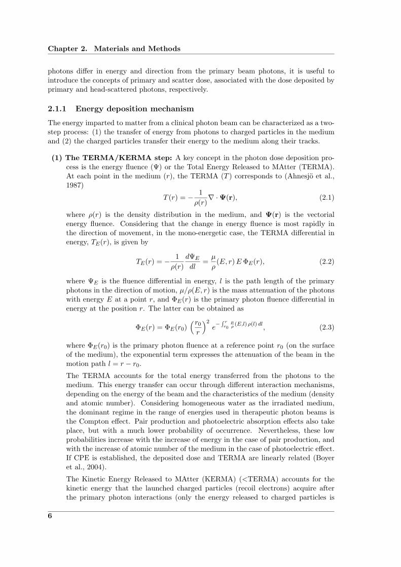
(1) The TERMA/KERMA step: A key concept in the photon dose deposition pro-cess is the energy fluence (Ψ) or the Total Energy Released to MAtter (TERMA).At each point in the medium (r), the TERMA (T ) corresponds to (Ahnesjo et al.,1987)
T (r) = − 1ρ(r)∇ ·Ψ(r), (2.1)
where ρ(r) is the density distribution in the medium, and Ψ(r) is the vectorialenergy fluence. Considering that the change in energy fluence is most rapidly inthe direction of movement, in the mono-energetic case, the TERMA differential inenergy, TE(r), is given by
TE(r) = − 1ρ(r)
dΨE
dl=µ
ρ(E, r)E ΦE(r), (2.2)
where ΨE is the fluence differential in energy, l is the path length of the primaryphotons in the direction of motion, µ/ρ(E, r) is the mass attenuation of the photonswith energy E at a point r, and ΦE(r) is the primary photon fluence differential inenergy at the position r. The latter can be obtained as
ΦE(r) = ΦE(r0)(r0r
)2e−∫ rr0
µρ(E,l) ρ(l) dl
, (2.3)
where ΦE(r0) is the primary photon fluence at a reference point r0 (on the surfaceof the medium), the exponential term expresses the attenuation of the beam in themotion path l = r − r0.
The TERMA accounts for the total energy transferred from the photons to themedium. This energy transfer can occur through different interaction mechanisms,depending on the energy of the beam and the characteristics of the medium (densityand atomic number). Considering homogeneous water as the irradiated medium,the dominant regime in the range of energies used in therapeutic photon beams isthe Compton effect. Pair production and photoelectric absorption effects also takeplace, but with a much lower probability of occurrence. Nevertheless, these lowprobabilities increase with the increase of energy in the case of pair production, andwith the increase of atomic number of the medium in the case of photoelectric effect.If CPE is established, the deposited dose and TERMA are linearly related (Boyeret al., 2004).
The Kinetic Energy Released to MAtter (KERMA) (<TERMA) accounts for thekinetic energy that the launched charged particles (recoil electrons) acquire afterthe primary photon interactions (only the energy released to charged particles is
6
2.2. Dose calculation methods: general aspects
accounted). Most of this energy is deposited quasi-locally due to multiple Coulombcollisions with neighboring orbital electrons or atomic nuclei (collision KERMA).However, a small fraction of the energy will be carried away from the primary in-teraction site through radiative events such as bremsstrahlung and electron-positronannihilation (radiative KERMA). The collision KERMA accounts for the first partof the energy deposition mechanism: the energy transfer from non-charged particlesto charged particles.
(2) The DOSE step: The inelastic collisions, in which a secondary electron transferssome of its energy to an orbital electron, represent the final mechanism of dosedeposition in matter. The amount of energy transferred to the orbital electron willproduce the excitation or ionization of the atom. If ionization occurs, the liberatedelectron will continue the process of excitation/ionization of atoms in its track untilit stops, when all its kinetic energy is lost.
2.1.2 Charge particle equilibrium
By definition, CPE exists for a volume v if every charged particle of a given type andenergy leaving v is replaced by an identical particle of the same energy entering it (Bergerand Seltzer, 1982). Under these conditions, the primary dose becomes exactly equal tothe collision KERMA.
To achieve a perfect CPE state using clinical photon beams is virtually impossible.The condition of CPE is lost in regions very close to the radiation source, the fluence willnot be uniform due to the 1/r2 factor accounting for the divergence of the beam, or closeto the interface between two materials of very different densities (e.g., tissue/air or soft-tissue/bone). The CPE is also lost when there is a magnetic or electric field induced thatdeviates the charged particles from their original path (valid for some radiation detectors)or for high energy radiation, as used in therapeutic photon beams (Hobbie and Roth, 2007).Easier to achieve is a state of transient-CPE that occurs when the energy deposited in themedium is proportional to the kinetic energy transferred to it. This condition is fulfilledin regions deeper than zmax, which corresponds to the forward range of the secondaryelectrons liberated from the primary photon interactions. From here on, the state oftransient-CPE will be referred to just as CPE.
Dose calculation algorithms often assume a state of CPE simplify the calculations.The simplification is achieved by performing a so-called KERMA-approximation. In con-ventional 3DCRT, this assumption is valid in most of the cases as the field sizes used arebig enough to provide this condition within the treated volumes. However, for narrowphoton beams this approximation can be too coarse and may produce calculated distribu-tions that do not reflect the delivered dose. As discussed by Das et al. (2008), the criticalparameter to CPE condition is, rather than the forward range of the secondary electrons,their lateral range (corresponding to approximately 1/3 to 1/2 of the forward range forenergies lower than 10 MV, Boyer et al. 2004).
2.2 Dose calculation methods: general aspects
In this section, a summary of the dose calculation concepts relevant to this thesis ispresented. For a comprehensive review on dose calculation methods see Ahnesjo andAspradakis (1999) or Boyer et al. (2004).
7
Chapter 2. Materials and Methods
In order to anticipate the outcome of a radiation treatment, it is necessary to performdose calculations. This should allow to determine the geometrical distribution and homo-geneity of the dose to be delivered to the patient, ensuring a good coverage of the targetand sparing of the organs at risk. The main requirements of the dose calculation algo-rithms are: high reliability, precision and accuracy in the determination of the dose, andhigh calculation speed (Schlegel and Mahr, 2007), if the purpose is treatment planning.
In earlier times, physicists manually calculated the dose to be delivered to the patient.These calculations were based on a set of beam parameters measured at different depthsin a water phantom for quadratic fields and in the use of empirical formulas (Day, 1950)to correct for the differences between the water tank and the patient. These methods werecalled factor-based methods (also called correction-based methods).
The use of computerized methods to calculate dose distributions, started with theadvent of CT. CT allows to obtain quantitative data on the anatomy of the patient, par-ticularly on the different electron densities of the tissues (associated with the HounsfieldUnits (HU)), which yielded an improvement on the geometrical accuracy of the calcula-tions. With the increase of computing power, more sophisticated calculation methods weredeveloped based on physical models. They are therefore called model-based algorithms.These methods, handle the primary and scatter components of the beam separately, usingphysical models of the beam and the deposition of energy in matter. Hence, they providea good description of the changes in scattering due to variations in the beam shape andpatient anatomy (Jelen, 2007).
2.2.1 Factor-based calculations
In the factor-based algorithms (Cunningham, 1972; Thames, 1973; Sontag and Cunning-ham, 1977; Sontag et al., 1977; Sontag and Cunningham, 1978; El-Khatib and Battista,1984) the dose is calculated by the multiplication of different factors that account forvariations from the reference conditions (beam modifications and patient-related mod-ifications) without explicit modeling of the transport of secondary electrons. The fac-tors used for the determination of the dose include: Off-Axis Ratios (OARs), OutputFactors (OFs), Percentage Depth Doses (PDDs), Tissue Air Ratios (TARs) and TissuePhantom Ratios (TPRs), among others.
Factor based methods offer a conceptually simple approach to calculate dose distribu-tions that has been widely used over the years for independent dose verification. However,there are some practical issues concerning this approach. The most important of themis that it is time consuming to measure all the parameters required to obtain a completetabulated data set, which covers the entire range of possible configurations to be evalu-ated. Nevertheless, if the intended use of the method is to evaluate the dose in regionsclose to the central axis for simple field shapes, this approach can certainly be used. Onthe other hand, if one wants to evaluate the dose at arbitrary positions using complexfield configurations (as commonly used in IMRT), the amount of data to be measured inorder to cover the complete range of possible configurations becomes prohibitively large(Olofsson, 2006).
Facing the huge flexibility in the dose delivery of TomoTherapy, it was decided not touse the correction-based method for the dose calculations. Instead, a more sophisticatedmodel-based method was used.
8

2.2. Dose calculation methods: general aspects
2.2.2 Model-based calculations
Within the model-based algorithms to calculate dose, two categories can be distinguished:the Monte Carlo calculations (highest accuracy, but long computation time) and the so-called kernel-based or convolution/superposition algorithms (Mackie et al., 1985). Kernel-based methods can model dose distributions very accurately and have the advantage ofbeing faster than the Monte Carlo methods. In kernel-based methods, the delivered dose isassumed to be equal to the sum (or superposition) of elementary photon beam components.The distribution of energy imparted to a medium after the interaction with an elementarybeam is called “kernel”, hence, the name of the method. In this kind of calculations, twocomponents are defined: (i) a primary (or ray tracing) component, which considers theenergy transferred to the medium by photons and (ii) a secondary component, which bringsinto effect the transport and deposition of energy by the secondary particles. The primarycomponent contains all the information regarding the beam shape and modulation, forwhich the geometry of the radiation system needs to be known. The other component isassumed to be independent from the geometric configuration of the system; it only dependson the spectrum of the photons and on the composition of the irradiated medium.
Depending on the “geometry” of the elementary beam, the kernel can receive differentnames. The most frequently used kernels are: the point-kernel (Figure 2.1(a)), whichdescribes the deposition of energy after a single (mono-energetic) photon interaction in thecenter of an infinite medium, and the pencil-beam-kernel (Figure 2.1(b)), which describesthe deposition of energy after the interaction of an infinitely narrow beam (or a finite sizeelementary beam) with a semi-infinite homogeneous medium.
The first step in the point-kernel calculations is to obtain the energy released in themedium due to the primary photon interactions considering the attenuation of the beam(this step is applicable to every model-based calculation). The second step is to calculatethe dose by superposing the contributions of energy deposited around each interaction sitedescribed by the kernel. The kernels are usually calculated for mono-energetic beams, soknowledge on the beam spectrum is required. Although this concept is simple, there aremany issues related to the implementation of this algorithm, including: long computationtimes, spectral variations, kernel variations due to heterogeneities and interpolation prob-lems. Some of these problems (particularly the computation time) are solved by parame-terizing point-kernels into conical sectors; this is the so-called “collapsed cone convolutionapproximation” (Ahnesjo, 1989).
A simpler and faster approach is used in the pencil-kernel calculations. The problemis reduced by one dimension, as the point kernels are already pre-summed in the direc-tion of the incident beam. Using this method, the dose is computed by obtaining thefluence/TERMA (Figure 2.1(c)) over the field opening and then integrating the kernelcontributions (Figure 2.1(d)). If the spectrum of the beam is not available, broad beamdata can be used for the determination of the correct weighting of the mono-energeticcomponents of the kernel.
The major limitation of the pencil beam kernel approach is the poor modeling ofdelivered dose distributions in the presence of lateral inhomogeneities. The pencil beammethod can correct for the presence of inhomogeneities only in the forward directionby re-scaling the kernel. For the purpose of this work (implementation of a verificationtool for dose distributions delivered in a homogeneous phantom), this limitation does notpresent a problem. Therefore, due to the theoretical simplicity, the pencil beam kernelapproximation has been used as the dose calculation engine. All the distributions were
9

Chapter 2. Materials and Methods
(a) (b)
(c) (d)
Figure 2.1: Pencil beam kernel based dose calculation. (a) Mono-energetic point-kernel. (b) Poly-energetic pencil beam kernel, obtained after cumulating the point-kernels in depth, considering beam attenuation and spectrum weighting. (c) Fluencedistribution for an open field, considering beam divergence. (d) Dose distribution,considering the transport of the secondary particles (convolution between the fluenceand the pencil beam).
calculated using water as the absorbing medium.The Pencil Beam Kernel (PBK) can be obtained using different methods. These include
experimental approaches (Ceberg et al., 1996; Storchi and Woudstra, 1996), a parameter-ized form (Nyholm et al., 2006) and Monte Carlo methods (Mohan and Chui, 1987; Ahnesjoand Trepp, 1991; Ahnesjo et al., 1992; Bourland and Chaney, 1992). In this work, a MonteCarlo based method was used. As the direct integration of the kernel over the field can becomputationally exhaustive, it is assumed that the kernel distribution is space-invariant.Under this assumption, the calculation can be carried out using convolution techniquessuch as the Fast Fourier Transform (FFT) (Boyer and Mok, 1985), reducing significantlythe number of operations to be performed. The details of the implementation of the PBKinto the dose calculations are given in Sections 2.3.2 and 2.3.3.
PBK-based dose calculations (as any other model-based method) require an accuratedetermination of the lateral fluence distributions for the different field configurations. Toobtain these distributions, there is an important effect to consider: the presence (or ab-sence) of a flattening filter, used in most of the conventional linacs. This filter, as suggestedby its name, is designed to produce a “flat” dose distribution at a certain depth in a water
10
2.2. Dose calculation methods: general aspects
phantom for a reference field size. This is accomplished by reducing the photon fluence inthe central part of the beam, as a function of the off-axis distance, producing the so-called“horn-effect” (due to the resulting shape of the lateral fluence profiles for large fields, seeFigure 3.8(b)). The absence of flattening filter (applicable to the TomoTherapy system,see Section 2.4.2), on the other hand, will leave the fluence for an open field unmodified,producing a cone-shaped lateral fluence distribution, as shown in Figure 2.11(a). A sim-ple way to account for these filtering effects is to obtain a fluence profile for the biggestfield size available and assume radial symmetry on the fluence distribution. The lateralphoton fluence can be determined by taking into account, besides the filtering effect, thegeometrical shape of the beam (for a given MLC/Jaws configuration), the effect of thespatial extension of the source and the head scatter contributions.
The scatter fraction coming from the treatment head can significantly contribute tothe treatment beam. In this work, the head scatter contribution has been considered inthe implementation of the “extended source” (that takes into account the focal spot sizeand the head scatter contributions, see Section 2.3.1). Nilsson and Brahme (1981) werethe first to identify the sources of such contributions. These are: the scatter from primarycollimators, the flattening filter, back-scatter to the monitor and forward-scatter from thesecondary collimators.
Second order effects in the dose calculation engine are the spectral changes of the beam(e.g., off-axis softening) and kernel tilting to account for the beam divergence. The mainreason for the spectral variations at off-axis positions is the flattening filter. Even though aconventional linac (which has a flattening filter) was used to validate the dose calculations,no corrections to account for this effect have been done. The justification of this decisionis based on the consideration that this work aims to verify dose distributions delivered bythe TomoTherapy system which lacks a flattening filter. It has been shown by Sharpe andBattista (1993) that the assumption of a parallel kernel can lead to significant errors in thedetermination of the dose for extreme configurations (large field size, high energy and shortSource-Surface Distance (SSD)). However, they also found that this approximation wasaccurate enough in most of the clinically relevant configurations. Hence, no correctionsare applied to account for this effect either.
2.2.3 Uncertainty considerations
The formal definition of the “uncertainty” of a measurement is: parameter associatedwith the result of a measurement that characterizes the dispersion of a value that couldreasonably be attributed to the measurand (BIPM et al., 1995). Uncertainties are classifiedeither as type A, if they can be assessed by statistical methods, or type B, if the assessmentcan not be done in a statistical way. Regardless of the method used for the determinationof the uncertainties, if there is more than one parameter involved in the determination ofa process, the individual uncertainties are usually combined in quadrature to estimate theoverall value.
The accuracy requirements of the delivered dose in radiotherapy are related to thetumor and normal tissue reactions. It has been recommended that the overall uncertaintyin the delivered dose to the patient should be less than 3-5% (1 Standard Deviation (SD))(ICRU, 1976; Dutreix, 1984; Mijnheer et al., 1987). Many analyzes have shown that thisis not an easy goal to achieve. From this fact arises the importance of the QA program,responsible for maintaining every step of the process within an acceptable tolerance.
Recent developments in external radiation therapy such as IMRT and IGRT allow
11

Chapter 2. Materials and Methods
a very high conformity of the delivered dose to the target. However, large geometricaluncertainties are still associated to the delineation of the target volume and organs at risk(Leunens et al., 1993; Giraud et al., 2002). Therefore, very high demands on the precisedosimetric and geometrical determination of the dose delivered to the patient are set.Uncertainties in the dose determination can originate either from the (measured) inputdata required by the dose calculation algorithm, or from the algorithm itself, i.e., poormodeling, inadequate approximations, coarse calculation grid size and other limitationsassociated with either the basic algorithm or its use (Fraass et al., 1998).
In order to estimate the uncertainty requirements specifically for the dose calculationprocess, two approaches can be used. In the ideal case, the requirement should be derivedfrom radiobiological data, according to the effect of dose variations in tumoral and normalcells. However, it is difficult to obtain quantitative data that can be used for this purpose,due to insufficient experiments and the variability in the tumor/tissue response to radi-ation (Boyer et al., 2004) among others. A more practical way to estimate the accuracyrequirements of the dose calculation by itself is to identify and quantify the uncertaintiesassociated with the dose delivery chain (Mijnheer et al., 1987; Ahnesjo and Aspradakis,1999; Boyer et al., 2004), which results in a variety of criteria. Given the complexity ofthe plans and the dosimetric issues, there are no specific dose accuracy recommendationsfor IMRT. The AAPM guidelines (Ezzell et al., 2003) suggest that for single beams in lowgradient regions, the agreement with measurements should be as good as it is required forconventional treatments (i.e., 2-4%). For typical complete treatment plans, the agreementwith the measurement should be within 3-4% in high dose low gradient regions.
The acceptance criteria used in radiotherapy are often expressed (in terms of 1 SD) asa combination of dose deviation, in low dose gradient regions, and Distance To Agreement(DTA), in high dose gradient regions. These criteria are adopted simply because in re-gions with high dose gradients a small displacement results in a large dose deviation. Theconverse is valid for the geometrical DTA criterion. One way to asses these criteria isto calculate both of them individually and then select the smaller value for each evalua-tion point. A more practical approach, widely used in the evaluation of calculated dosedistributions, is the gamma index concept developed by Low, Harms, Mutic and Purdy(1998). This concept combines the dose difference (global or local, as desired) and thespatial distance between the measured and evaluated points in a dose-distance space. Themeasure of acceptance is the multidimensional distance between measured and calculatedvalues in the dose-distance space, scaled by the individual acceptance criteria. In the caseof a 2-dimensional distribution, the acceptance criterion corresponds to the surface of anellipsoid in the dose-distance space centered in the measured value to be evaluated. Theresolution of the evaluated distribution should be 1/3 of the DTA criterion according toLow and Dempsey (2003), implying that the evaluation data may need to be interpolated.For clinical dose verification a combination of 3-5% dose difference and 3 mm DTA iscommonly used (Low, Harms, Mutic and Purdy, 1998; Low and Dempsey, 2003; Winkleret al., 2005; Childress et al., 2005; Thomas et al., 2005; van Zijtveld et al., 2006).
The dosimetric uncertainties can be associated with the detector/readout system’ssensitivity and response issues, output stability of the radiation system and geometricalinaccuracies in the alignment of the beam with the detector and/or the phantom.
12

2.3. Dose calculation method: establishment of a model applicable to smallbeams
2.3 Dose calculation method: establishment of a model ap-plicable to small beams
Small fields, i.e., fields with a size comparable or smaller than the lateral range of asso-ciated secondary electrons, are increasingly used in radiotherapy. The most prominentexample is their application in stereotactic radiosurgery. However, this statement alsoapplies to larger fields that are composed of small beams, as used in IMRT. This has beenparticularly promoted by the clinical availability of recent developments, such as mini- ormicro- MLCs on conventional accelerators and treatment units specifically designed forstereotaxy (GammaKnife, CyberKnife) or intensity modulated treatments (TomoTher-apy).
A versatile model of small beams needs to overcome two problems:
(1) As long as the number of possible shapes of different small fields remains small (as itis the case for radiosurgery using a set of cylindrical collimators), the beam modelrequired for dose calculation can simply be based on experimental input data suchas PDDs, profiles or output factors for a small set of small fields. However, forIMRT, with an almost unlimited number of different small field shapes (patterns),it is difficult to apply the same approach.
(2) A beam model for small fields must be validated by experimental results, however,dosimetry of small fields is still a challenge. High dose gradients set constraints on thedetector size, furthermore, composition effects and small positioning errors becomerelevant (Pappas et al., 2008; Das et al., 2008; Alfonso et al., 2008). Therefore,the use of new techniques has increased the uncertainty in clinical dosimetry. Oneexample of this is the introduction of systematic errors in the treatment planningimplementation, due to inaccuracies in the small field measurements (Crop et al.,2007). Additionally, for certain techniques, it has become very difficult, or even notpossible (e.g., TomoTherapy), to perform reference dosimetry based on the availabledosimetry protocols. These issues have concerned international organizations suchas the International Atomic Energy Agency (IAEA). Indeed, efforts are currentlybeing made by the IAEA to set the basis of new international recommendations inorder to standardize the dosimetry for the new delivery techniques (Alfonso et al.,2008).
The model presented in this section explicitly takes into account the two main effectsaffecting the dose distributions for small field sizes. These are: (i) the fact that the sourceof radiation is not point-like but extended in space and that the partial blocking of it willhave an impact on the penumbra of the field and beam output (Scott et al., 2008) and(ii) the lack of CPE conditions within the field when its size is comparable to the lateralrange of the secondary electrons in the medium (Das et al., 2008). Considering the knowngeometry of the system and these two effects, lateral dose distributions and output factorsin water can be well modeled by convolution techniques (Mackie et al., 1985).
The validation of the beam model was performed using a 6 MV photon beam of aSiemens Primus linac. Comparisons of measured versus calculated output factors anddose profiles are presented as tests of the algorithm.
This section is based on an article that has been published in a peer-reviewed journal(Caprile and Hartmann, 2009).
13

Chapter 2. Materials and Methods
2.3.1 Determination of the spatial extension of the source
Several techniques for the determination of the intensity distribution of the radiationsource have been used in the past (Munro et al., 1988; Treuer et al., 1993; Yang et al.,2002; Treuer et al., 2003; Yan et al., 2008), but perhaps the only one out of these thatallows a quantitative and direct reconstruction of the source distribution is the “slit-method” presented by Munro et al. in 1988. This technique, coupled with an analysis ofCollimator Factors (CFs) (output factors measured free in air), was used to reconstructthe “extended source” of the linac.
The extended source is defined as the projection of all primary photons and head scattercontributions into a common plane, perpendicular to the axis of the beam and located atthe source position. This two-dimensional distribution is composed of an “inner” andan “outer” part. The inner part (focal spot) can be reconstructed by the slit-method.The outer part cannot be directly obtained from such measurements due to its very lowcontribution compared with the inner part. Therefore, it was indirectly determined fromCFs measurements, assuming that the observed increase of the CFs with the field size canbe attributed to photons originating from the extended source.
Inner part
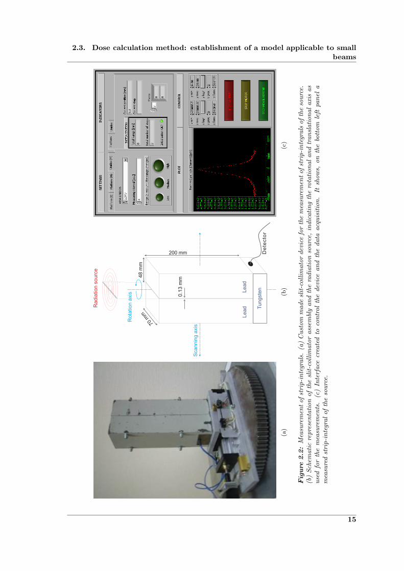
The reconstruction of the focal spot is based on the measurement of strip-integrals ofthe source and the use of image reconstruction techniques (Munro et al., 1988). Theprinciple is that using a slit-collimator and a radiation detector, it is possible to measurethe radiation coming from a very small slit of the source (emitted in the forward direction).If this measurement is repeated at different positions, by linearly moving the collimator anddetector in the direction perpendicular to the slit, a strip-integral of the source is obtained(an example strip-integral can be seen in the scatter plot shown in Figure 2.2(c)). Now,by measuring strip-integrals of the source at different angles (with the center of rotationaligned with the central axis of the beam) and making use of the central slice theorem(Gaskill, 1978) or other CT image reconstruction technique, it is possible to obtain theshape and size of the source.
The device used for the measurement of the strip-integrals (shown in Figure 2.2(a))is composed of two slabs of lead/antimony of 200x70x48 mm3 separated by a distance of130 µm, forming a slit-collimator. A block of tungsten, with a drilled hole and an openingonly in the direction towards the slit, is attached under the slit-collimator. It contains asolid state detector (diode type p, Model 6008, PTW Freiburg, Germany). The assemblyis mounted on a dynamic base that can be moved linearly in steps of 0.05 mm with atotal range of 4 cm. The base is fixed to a platform that can rotate 180◦ on its own axisin 3◦ steps. The field of view of the detector, as seen in Figure 2.2(b), is limited to theprojection of the slit into the source plane.
The device was remotely controlled by a portable computer using a tool programmedwith LabVIEW 8.2 (National Instruments Corporation, Austin, TX, USA) in the “G”programming language. This tool can synchronize the movement of the stage with themeasurement of the diode for the selected integration time (Figure 2.2(c)). The detectorposition, the integration time and the measured charge at each scanning point are storedin an ASCII file for later processing and analysis. A scanning range of 40 mm, a stepsize of 0.1 mm and an integration time of 1 s were used for the measurement of the strip-integrals. The collimator was positioned with the top side at a distance of approximately
14
2.3. Dose calculation method: establishment of a model applicable to smallbeams
(a)
(b)
(c)
Fig
ure
2.2
:M
easu
rem
ent
ofst
rip-
inte
gral
s.(a
)C
usto
mm
ade
slit
-col
limat
orde
vice
for
the
mea
sure
men
tof
stri
p-in
tegr
als
ofth
eso
urce
.(b
)Sc
hem
atic
repr
esen
tati
onof
the
slit
-col
limat
oras
sem
bly
and
the
radi
atio
nso
urce
,in
dica
ting
the
rota
tion
alan
dtr
ansl
atio
nala
xis
asus
edfo
rth
em
easu
rem
ents
.(c
)In
terf
ace
crea
ted
toco
ntro
lth
ede
vice
and
the
data
acqu
isit
ion.
Itsh
ows,
onth
ebo
ttom
left
pane
la
mea
sure
dst
rip-
inte
gral
ofth
eso
urce
.
15

Chapter 2. Materials and Methods
50 cm from the source. The radiation field was set to a nominal value of 10x10 cm2 (atthe isocenter) for the linac and of 10x5 cm2 for TomoTherapy.
There are many algorithms used in CT image reconstruction (Kopka and Daly, 1977).All of them yield a representation of the object, from which the strip-integrals were taken,that is not exempt of artifacts. For the reconstruction of the two-dimensional distributionof the focal spot, an iterative algorithm was selected. With this algorithm, it was easierto constrain the results to be physically valid, i.e., no negative values were allowed. Thealgorithm minimizes the function:
χ2(X) =∑km
(∑ij F
kmij Xij − pkm
)2
σ2km
, (2.4)
where pkm is the measured projection value at the mth angle and kth position with anuncertainty of σkm, Xij is the intensity of the focal spot in the pixel (i, j) at the sourceplane and F kmij is the fraction of Xij projected into pkm.
Even though the detector is embedded in a tungsten block, scattered radiation comingfrom parts other than the slit (e.g., room scatter) is detected by the diode, increasing themeasured signal from the source by an unknown amount. This effect is not negligible atthe “wings” of the strip-integral. Therefore, the reconstructed distribution was consideredto be part of the focal spot only down to ∼0.1% of the maximum intensity. The section ofthe reconstructed distribution where the intensity was less than ∼0.1% of the maximumwas considered to belong to the outer part of the source.
Outer part.
The outer part of the source was obtained by fitting the calculated CFs, or collimatorscatter factors (Sc) in Khan’s notation (Khan et al., 1980), to the measured values. Theunnormalized CFs were calculated simply as the integral of the “visible” part of the ex-tended source from the point of view of the detector, as follows
CF (Fx, Fy, lm) =∫ +limx
−limx
∫ +limy
−limyS(x′, y′) dx′ dy′, (2.5)
where Fx and Fy indicate the field size at the measurement plane in x and y directionrespectively, lm is the distance from the source to the detector (located on the central axisof the beam) and S is the two-dimensional intensity distribution of the extended source.limx and limy are the integration limits, defined by the projection of the collimator edgesto the source plane. This projection requires that the positions of the collimators used toproduce the field are known. They are obtained simply as
limx =Fx2· lcxlm − lcx
limy =Fy2· lcylm − lcy
,
where lcx and lcy are the distances from the source to the closer edges of the MLC andthe Y-Jaws respectively.
16
2.3. Dose calculation method: establishment of a model applicable to smallbeams
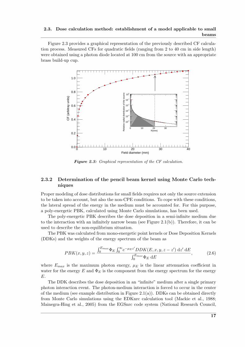
Figure 2.3 provides a graphical representation of the previously described CF calcula-tion process. Measured CFs for quadratic fields (ranging from 2 to 40 cm in side length)were obtained using a photon diode located at 100 cm from the source with an appropriatebrass build-up cup.
1.0
0.8
0.6
0.4
0.2
0.0403020100
CF
(ar
bitr
ay u
nits
)
Field diameter (mm)
100
10-1
10-2
10-3
10-4
10-5
3020100
Rel
ativ
e ra
dial
dis
trib
utio
n of
the
sour
ce
R(mm)
Figure 2.3: Graphical representation of the CF calculation.
2.3.2 Determination of the pencil beam kernel using Monte Carlo tech-niques
Proper modeling of dose distributions for small fields requires not only the source extensionto be taken into account, but also the non-CPE conditions. To cope with these conditions,the lateral spread of the energy in the medium must be accounted for. For this purpose,a poly-energetic PBK, calculated using Monte Carlo simulations, has been used.
The poly-energetic PBK describes the dose deposition in a semi-infinite medium dueto the interaction with an infinitely narrow beam (see Figure 2.1(b)). Therefore, it can beused to describe the non-equilibrium situation.
The PBK was calculated from mono-energetic point kernels or Dose Deposition Kernels(DDKs) and the weights of the energy spectrum of the beam as
PBK(x, y, z) =
∫ Emax0 ΦE
∫∞0 e−µEz
′DDK(E, x, y, z − z′) dz′ dE∫ Emax
0 ΦE dE, (2.6)
where Emax is the maximum photon energy, µE is the linear attenuation coefficient inwater for the energy E and ΦE is the component from the energy spectrum for the energyE.
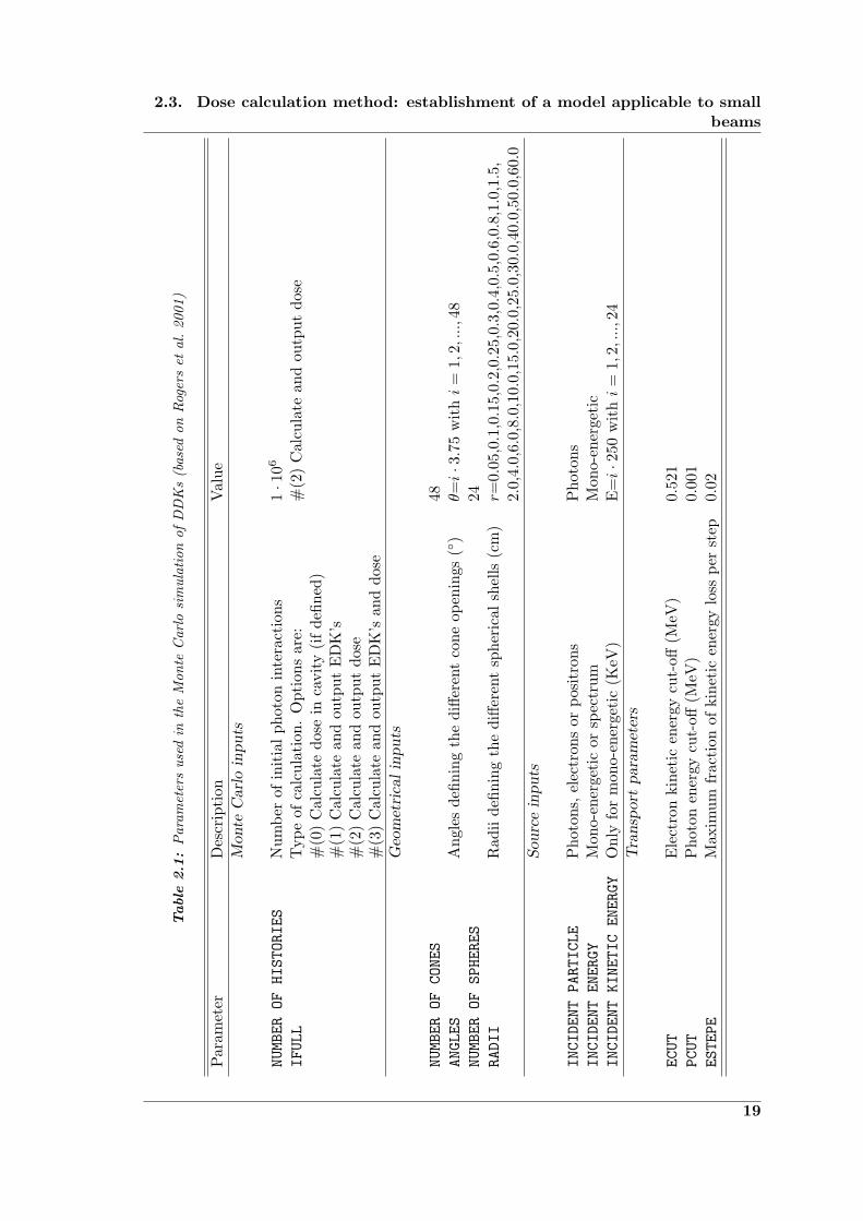
The DDK describes the dose deposition in an “infinite” medium after a single primaryphoton interaction event. The photon-medium interaction is forced to occur in the centerof the medium (see example distribution in Figure 2.1(a)). DDKs can be obtained directlyfrom Monte Carlo simulations using the EDKnrc calculation tool (Mackie et al., 1988;Mainegra-Hing et al., 2005) from the EGSnrc code system (National Research Council,
17
Chapter 2. Materials and Methods
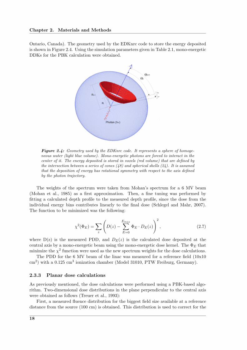
Ontario, Canada). The geometry used by the EDKnrc code to store the energy depositedis shown in Figure 2.4. Using the simulation parameters given in Table 2.1, mono-energeticDDKs for the PBK calculation were obtained.
Figure 2.4: Geometry used by the EDKnrc code. It represents a sphere of homoge-neous water (light blue volume). Mono-energetic photons are forced to interact in thecenter of it. The energy deposited is stored in voxels (red volume) that are defined bythe intersection between a series of cones (48) and spherical shells (24). It is assumedthat the deposition of energy has rotational symmetry with respect to the axis definedby the photon trajectory.
The weights of the spectrum were taken from Mohan’s spectrum for a 6 MV beam(Mohan et al., 1985) as a first approximation. Then, a fine tuning was performed byfitting a calculated depth profile to the measured depth profile, since the dose from theindividual energy bins contributes linearly to the final dose (Schlegel and Mahr, 2007).The function to be minimized was the following:
χ2(ΦE) =∑z
(D(z)−
Emax∑E=0
ΦE ·DE(z)
)2
, (2.7)
where D(z) is the measured PDD, and DE(z) is the calculated dose deposited at thecentral axis by a mono-energetic beam using the mono-energetic dose kernel. The ΦE thatminimize the χ2 function were used as the new spectrum weights for the dose calculations.
The PDD for the 6 MV beam of the linac was measured for a reference field (10x10cm2) with a 0.125 cm3 ionization chamber (Model 31010, PTW Freiburg, Germany).
2.3.3 Planar dose calculations
As previously mentioned, the dose calculations were performed using a PBK-based algo-rithm. Two-dimensional dose distributions in the plane perpendicular to the central axiswere obtained as follows (Treuer et al., 1993):
First, a measured fluence distribution for the biggest field size available at a referencedistance from the source (100 cm) is obtained. This distribution is used to correct for the
18
2.3. Dose calculation method: establishment of a model applicable to smallbeams
Table
2.1
:P
aram
eter
sus
edin
the
Mon
teC
arlo
sim
ulat
ion
ofD
DK
s(b
ased
onR
oger
set
al.
2001
)
Par
amet
erD
escr
ipti
onV
alue
Mon
teC
arl
oin
pu
ts
NUMBEROFHISTORIES
Num
ber
ofin
itia
lph
oton
inte
ract
ions
1·1
06
IFULL
Typ
eof
calc
ulat
ion.
Opt
ions
are:
#(2
)C
alcu
late
and
outp
utdo
se#
(0)
Cal
cula
tedo
sein
cavi
ty(i
fde
fined
)#
(1)
Cal
cula
tean
dou
tput
ED
K’s
#(2
)C
alcu
late
and
outp
utdo
se#
(3)
Cal
cula
tean
dou
tput
ED
K’s
and
dose
Geo
met
rica
lin
pu
ts
NUMBEROFCONES
48ANGLES
Ang
les
defin
ing
the
diffe
rent
cone
open
ings
(◦)
θ=i·3.7
5w
ithi
=1,
2,...,
48NUMBEROFSPHERES
24RADII
Rad
iide
finin
gth
edi
ffere
ntsp
heri
cal
shel
ls(c
m)
r=0.
05,0
.1,0
.15,
0.2,
0.25
,0.3
,0.4
,0.5
,0.6
,0.8
,1.0
,1.5
,2.
0,4.
0,6.
0,8.
0,10
.0,1
5.0,
20.0
,25.
0,30
.0,4
0.0,
50.0
,60.
0S
ourc
ein
pu
ts
INCIDENTPARTICLE
Pho
tons
,el
ectr
ons
orpo
sitr
ons
Pho
tons
INCIDENTENERGY
Mon
o-en
erge
tic
orsp
ectr
umM
ono-
ener
geti
cINCIDENTKINETICENERGY
Onl
yfo
rm
ono-
ener
geti
c(K
eV)
E=i·2
50w
ithi
=1,
2,...,
24T
ran
spor
tp
aram
eter
s
ECUT
Ele
ctro
nki
neti
cen
ergy
cut-
off(M
eV)
0.52
1PCUT
Pho
ton
ener
gycu
t-off
(MeV
)0.
001
ESTEPE
Max
imum
frac
tion
ofki
neti
cen
ergy
loss
per
step
0.02
19
Chapter 2. Materials and Methods
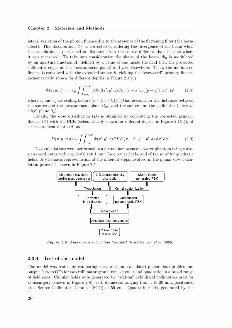
lateral variation of the photon fluence due to the presence of the flattening filter (the horn-effect). This distribution, Φ0, is corrected considering the divergence of the beam whenthe calculation is performed at distances from the source different than the one whereit was measured. To take into consideration the shape of the beam, Φ0 is modulatedby an aperture function A: defined by a value of one inside the field (i.e., the projectedcollimator edges at the measurement plane) and zero elsewhere. Then, the modulatedfluence is convolved with the extended source S, yielding the “corrected” primary fluence(schematically shown for different depths in Figure 2.1(c))
Φ(x, y, z) = cxcy
∫ ∫ +∞
−∞[AΦ0](x′, y′, z)S(cx[x− x′], cy[y − y′]) dx′ dy′, (2.8)
where cx and cy are scaling factors (c = (lm−lc)/lc) that account for the distances betweenthe source and the measurement plane (lm) and the source and the collimator (effectiveedge) plane (lc).
Finally, the dose distribution (D) is obtained by convolving the corrected primaryfluence (Φ) with the PBK (schematically shown for different depths in Figure 2.1(d)), ata measurement depth (d) as
D(x, y, z; d) =∫ ∫ +∞
−∞Φ(x′, y′, z)PBK(x− x′, y − y′, d) dx′ dy′. (2.9)
Dose calculations were performed in a virtual homogeneous water phantom using carte-sian coordinates with a grid of 0.1x0.1 mm2 for circular fields, and of 1x1 mm2 for quadraticfields. A schematic representation of the different steps involved in the planar dose calcu-lation process is shown in Figure 2.5.
Figure 2.5: Planar dose calculation flowchart (based on Yan et al. 2008).
2.3.4 Test of the model
The model was tested by comparing measured and calculated planar dose profiles andoutput factors OFs for two collimator geometries: circular and quadratic, in a broad rangeof field sizes. Circular fields were generated by “add-on” cylindrical collimators used forradiosurgery (shown in Figure 2.6), with diameters ranging from 1 to 20 mm, positionedat a Source-Collimator Distance (SCD) of 59 cm. Quadratic fields, generated by the
20
2.3. Dose calculation method: establishment of a model applicable to smallbeams
inherent system (i.e., the MLC collimation in X direction and Y -jaws in the perpendiculardirection), ranged from 0.5 to 40 cm in side length. Measurements were performed in awater tank (Model MP3, PTW Freiburg, Germany) using a photon diode. Dose profilesand OFs were measured at a SSD of 100 cm, at 1.5 cm depth in water.
(a) (b)
(c) PTW c© (d) PTW c©
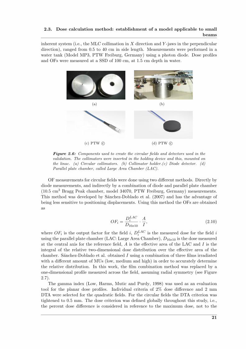
Figure 2.6: Components used to create the circular fields and detectors used in thevalidation. The collimators were inserted in the holding device and this, mounted onthe linac. (a) Circular collimators. (b) Collimator holder.(c) Diode detector. (d)Parallel plate chamber, called Large Area Chamber (LAC).
OF measurements for circular fields were done using two different methods. Directly bydiode measurements, and indirectly by a combination of diode and parallel plate chamber(10.5 cm3 Bragg Peak chamber, model 34070, PTW Freiburg, Germany) measurements.This method was developed by Sanchez-Doblado et al. (2007) and has the advantage ofbeing less sensitive to positioning displacements. Using this method the OFs are obtainedas
OFi =DLACi
D10x10· AI, (2.10)
where OFi is the output factor for the field i, DLACi is the measured dose for the field i
using the parallel plate chamber (LAC: Large Area Chamber), D10x10 is the dose measuredat the central axis for the reference field, A is the effective area of the LAC and I is theintegral of the relative two-dimensional dose distribution over the effective area of thechamber. Sanchez-Doblado et al. obtained I using a combination of three films irradiatedwith a different amount of MUs (low, medium and high) in order to accurately determinethe relative distribution. In this work, the film combination method was replaced by aone-dimensional profile measured across the field, assuming radial symmetry (see Figure2.7).
The gamma index (Low, Harms, Mutic and Purdy, 1998) was used as an evaluationtool for the planar dose profiles. Individual criteria of 2% dose difference and 2 mmDTA were selected for the quadratic fields. For the circular fields the DTA criterion wastightened to 0.5 mm. The dose criterion was defined globally throughout this study, i.e.,the percent dose difference is considered in reference to the maximum dose, not to the
21

Chapter 2. Materials and Methods
(a) (b)
Figure 2.7: OF measurement procedure using a combination of parallel plate cham-ber and diode. (a) Representation of the chamber positioning within the field (circle)and a cross-field profile (dashed line). (b) Representation of a cross-field profile mea-sured over the chamber area, used for the determination of the 2-D distribution (radialsymmetry).
local value.
2.4 Application to TomoTherapy: dose delivery verificationtool
A dose calculation tool to be used in the verification of TomoTherapy delivered dosedistributions was developed. The aim of this tool is for it to be implemented into the QAprogram of the system. It can also be used to study in depth the delivery technique andthe influence of the different parameters in the final distribution. For this, it is necessaryto understand the main characteristics of the delivery system that distinguish it fromconventional teletherapy units. Furthermore, the dosimetric issues and QA challengespresented by the novel components of helical TomoTherapy need to be described in orderto provide the context of this dose verification tool’s usefulness.
2.4.1 Independent dose verification
The main reason to implement a dose verification tool is to have a method, in addition tothe commercial TPS, to predict the outcome of a treatment. It is recommended (Kutcheret al., 1994) to verify the treatment parameters with an independent method, especiallywhen the modality of treatment is complex (e.g., TomoTherapy). In such cases, smallerrors in the treatment parameters could lead to more serious consequences in the per-formance of the overall treatment than in the case of simpler techniques. Moreover, it issuggested that the patient verification should include both dose calculations and deliveryverification measurements(Ezzell et al., 2003).
There are commercially available solutions for this purpose that can be used for con-ventional IMRT. However, the differences between the TomoTherapy delivery systemand conventional IMRT (see Section 2.4.2) make them inadequate to be used for doseverification in TomoTherapy(Gibbons et al., 2009).
22
2.4. Application to TomoTherapy: dose delivery verification tool
The dose verification tool developed allows to calculate distributions delivered by theTomoTherapy system to a homogeneous phantom, using input data that is independentof the TPS. This tool provides a supplemental QA procedure to verify the overall per-formance of the Hi·ART TomoTherapy system. Additionally, it allows to vary individualtreatment parameters. This feature is particularly useful to study the influence on theoverall treatment that the variation of parameters, such as output, gantry speed or couchvelocity, would have. The calculated results were compared to measurements in static anddynamic modes. The performance of this method in inhomogeneous media has not beeninvestigated yet and escapes from the scope of the presented work.
2.4.2 The Hi·ART TomoTherapy SystemR©
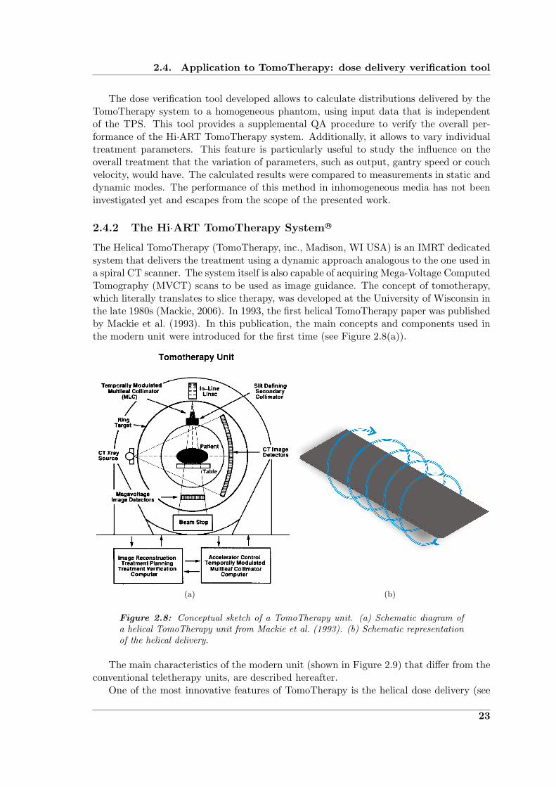
The Helical TomoTherapy (TomoTherapy, inc., Madison, WI USA) is an IMRT dedicatedsystem that delivers the treatment using a dynamic approach analogous to the one used ina spiral CT scanner. The system itself is also capable of acquiring Mega-Voltage ComputedTomography (MVCT) scans to be used as image guidance. The concept of tomotherapy,which literally translates to slice therapy, was developed at the University of Wisconsin inthe late 1980s (Mackie, 2006). In 1993, the first helical TomoTherapy paper was publishedby Mackie et al. (1993). In this publication, the main concepts and components used inthe modern unit were introduced for the first time (see Figure 2.8(a)).
(a) (b)
Figure 2.8: Conceptual sketch of a TomoTherapy unit. (a) Schematic diagram ofa helical TomoTherapy unit from Mackie et al. (1993). (b) Schematic representationof the helical delivery.
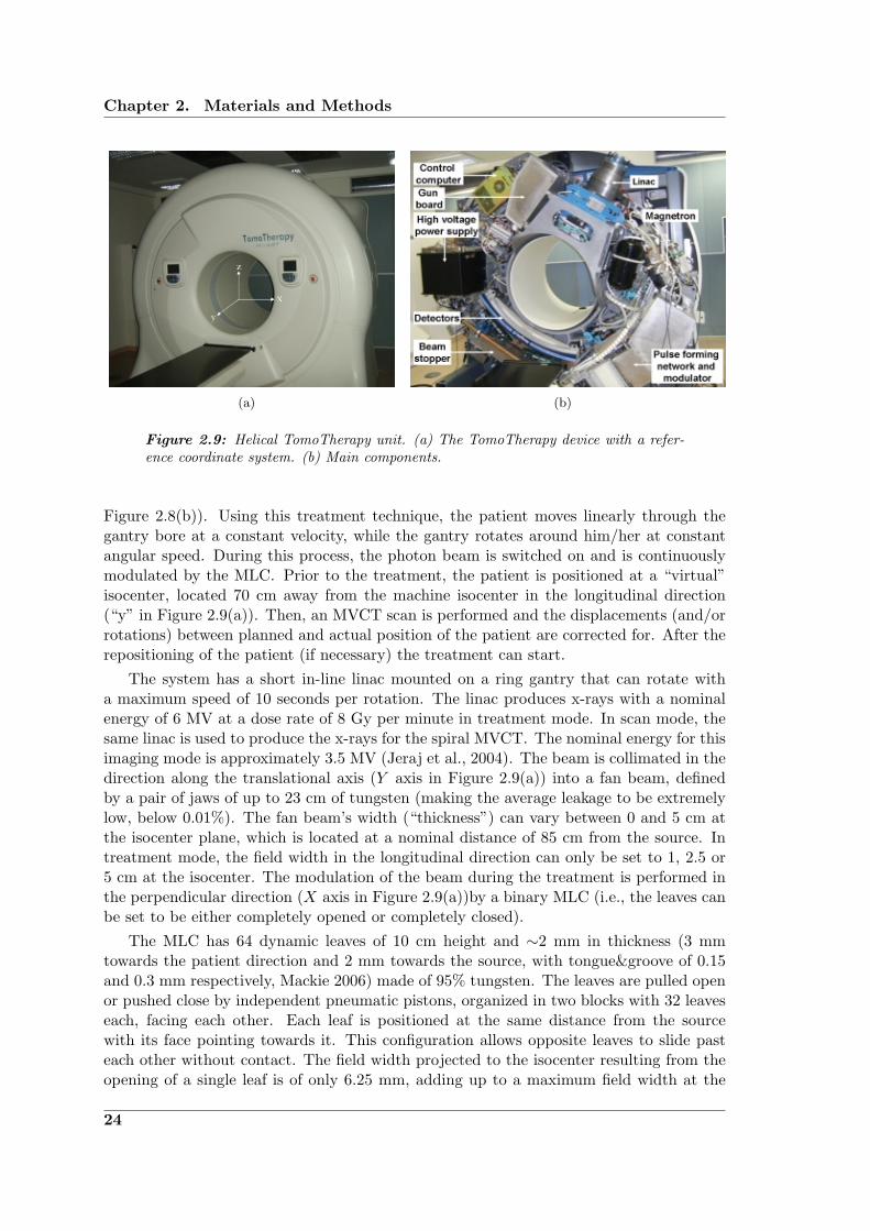
The main characteristics of the modern unit (shown in Figure 2.9) that differ from theconventional teletherapy units, are described hereafter.
One of the most innovative features of TomoTherapy is the helical dose delivery (see
23
Chapter 2. Materials and Methods
(a) (b)
Figure 2.9: Helical TomoTherapy unit. (a) The TomoTherapy device with a refer-ence coordinate system. (b) Main components.
Figure 2.8(b)). Using this treatment technique, the patient moves linearly through thegantry bore at a constant velocity, while the gantry rotates around him/her at constantangular speed. During this process, the photon beam is switched on and is continuouslymodulated by the MLC. Prior to the treatment, the patient is positioned at a “virtual”isocenter, located 70 cm away from the machine isocenter in the longitudinal direction(“y” in Figure 2.9(a)). Then, an MVCT scan is performed and the displacements (and/orrotations) between planned and actual position of the patient are corrected for. After therepositioning of the patient (if necessary) the treatment can start.
The system has a short in-line linac mounted on a ring gantry that can rotate witha maximum speed of 10 seconds per rotation. The linac produces x-rays with a nominalenergy of 6 MV at a dose rate of 8 Gy per minute in treatment mode. In scan mode, thesame linac is used to produce the x-rays for the spiral MVCT. The nominal energy for thisimaging mode is approximately 3.5 MV (Jeraj et al., 2004). The beam is collimated in thedirection along the translational axis (Y axis in Figure 2.9(a)) into a fan beam, definedby a pair of jaws of up to 23 cm of tungsten (making the average leakage to be extremelylow, below 0.01%). The fan beam’s width (“thickness”) can vary between 0 and 5 cm atthe isocenter plane, which is located at a nominal distance of 85 cm from the source. Intreatment mode, the field width in the longitudinal direction can only be set to 1, 2.5 or5 cm at the isocenter. The modulation of the beam during the treatment is performed inthe perpendicular direction (X axis in Figure 2.9(a))by a binary MLC (i.e., the leaves canbe set to be either completely opened or completely closed).
The MLC has 64 dynamic leaves of 10 cm height and ∼2 mm in thickness (3 mmtowards the patient direction and 2 mm towards the source, with tongue&groove of 0.15and 0.3 mm respectively, Mackie 2006) made of 95% tungsten. The leaves are pulled openor pushed close by independent pneumatic pistons, organized in two blocks with 32 leaveseach, facing each other. Each leaf is positioned at the same distance from the sourcewith its face pointing towards it. This configuration allows opposite leaves to slide pasteach other without contact. The field width projected to the isocenter resulting from theopening of a single leaf is of only 6.25 mm, adding up to a maximum field width at the
24
2.4. Application to TomoTherapy: dose delivery verification tool
isocenter of 40 cm (64 leaves opened) in the transverse (X) direction. The transit time ofthe MLC leaves is of only 20 ms.
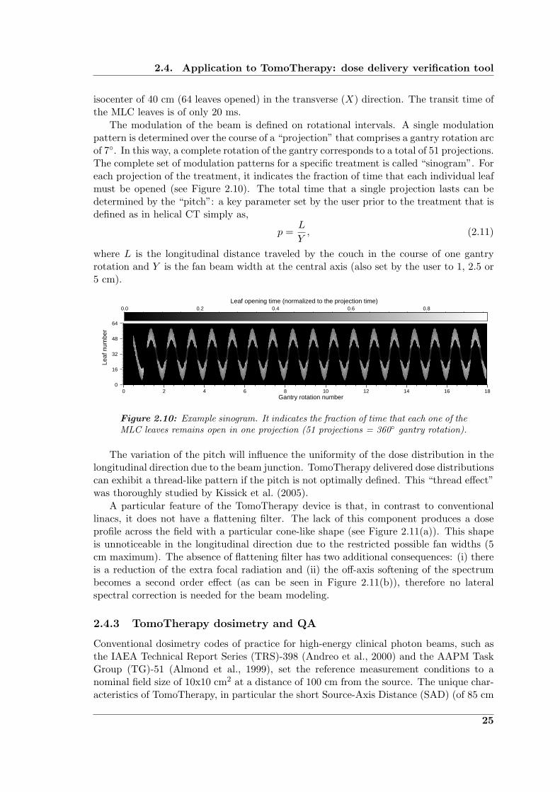
The modulation of the beam is defined on rotational intervals. A single modulationpattern is determined over the course of a “projection” that comprises a gantry rotation arcof 7◦. In this way, a complete rotation of the gantry corresponds to a total of 51 projections.The complete set of modulation patterns for a specific treatment is called “sinogram”. Foreach projection of the treatment, it indicates the fraction of time that each individual leafmust be opened (see Figure 2.10). The total time that a single projection lasts can bedetermined by the “pitch”: a key parameter set by the user prior to the treatment that isdefined as in helical CT simply as,
p =L
Y, (2.11)
where L is the longitudinal distance traveled by the couch in the course of one gantryrotation and Y is the fan beam width at the central axis (also set by the user to 1, 2.5 or5 cm).
64
48
32
16
0181614121086420
0.80.60.40.20.0Leaf opening time (normalized to the projection time)
Leaf
num
ber
Gantry rotation number
Figure 2.10: Example sinogram. It indicates the fraction of time that each one of theMLC leaves remains open in one projection (51 projections = 360◦ gantry rotation).
The variation of the pitch will influence the uniformity of the dose distribution in thelongitudinal direction due to the beam junction. TomoTherapy delivered dose distributionscan exhibit a thread-like pattern if the pitch is not optimally defined. This “thread effect”was thoroughly studied by Kissick et al. (2005).
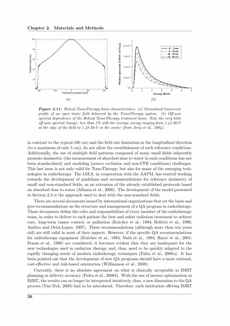
A particular feature of the TomoTherapy device is that, in contrast to conventionallinacs, it does not have a flattening filter. The lack of this component produces a doseprofile across the field with a particular cone-like shape (see Figure 2.11(a)). This shapeis unnoticeable in the longitudinal direction due to the restricted possible fan widths (5cm maximum). The absence of flattening filter has two additional consequences: (i) thereis a reduction of the extra focal radiation and (ii) the off-axis softening of the spectrumbecomes a second order effect (as can be seen in Figure 2.11(b)), therefore no lateralspectral correction is needed for the beam modeling.
2.4.3 TomoTherapy dosimetry and QA
Conventional dosimetry codes of practice for high-energy clinical photon beams, such asthe IAEA Technical Report Series (TRS)-398 (Andreo et al., 2000) and the AAPM TaskGroup (TG)-51 (Almond et al., 1999), set the reference measurement conditions to anominal field size of 10x10 cm2 at a distance of 100 cm from the source. The unique char-acteristics of TomoTherapy, in particular the short Source-Axis Distance (SAD) (of 85 cm
25
Chapter 2. Materials and Methods
100
80
60
40
20
2001000-100-200
Rel
ativ
e do
se [%
]
Transverse position [mm]
(a) (b)
Figure 2.11: Helical TomoTherapy beam characteristics. (a) Normalized transverseprofile of an open static field delivered by the TomoTherapy system. (b) Off-axisspectral dependence of the Helical TomoTherapy treatment beam. Note the very littleoff-axis spectral change: less than 5% with the average energy ranging from 1.43 MeVat the edge of the field to 1.49 MeV in the center (from Jeraj et al., 2004).
in contrast to the typical 100 cm) and the field size limitation in the longitudinal direction(to a maximum of only 5 cm), do not allow the establishment of such reference conditions.Additionally, the use of multiple field patterns composed of many small fields inherentlypresents dosimetric (the measurement of absorbed dose to water in such conditions has notbeen standardized) and modeling (source occlusion and non-CPE conditions) challenges.This last issue is not only valid for TomoTherapy, but also for many of the emerging tech-nologies in radiotherapy. The IAEA, in cooperation with the AAPM, has started workingtowards the development of guidelines and recommendations for reference dosimetry ofsmall and non-standard fields, as an extension of the already established protocols basedon absorbed dose to water (Alfonso et al., 2008). The development of the model presentedin Section 2.3 is the approach used to deal with the non-standard fields.
There are several documents issued by international organizations that set the basis andgive recommendations on the structure and management of a QA program in radiotherapy.These documents define the roles and responsibilities of every member of the radiotherapyteam, in order to deliver to each patient the best and safest radiation treatment to achievecure, long-term tumor control, or palliation (Kutcher et al., 1994; Belletti et al., 1996;Andreo and Ortiz-Lopez, 1997). These recommendations (although more than ten yearsold) are still valid in most of their aspects. However, if the specific QA recommendationsfor radiotherapy equipment (Kutcher et al., 1994; Nath et al., 1994; Boyer et al., 2001;Fraass et al., 1998) are considered, it becomes evident that they are inadequate for thenew technologies used in radiation therapy and, thus, need to be quickly adapted to therapidly changing needs of modern radiotherapy techniques (Palta et al., 2008a). It hasbeen pointed out that the development of new QA programs should have a more rational,cost-effective and risk-based orientation (Williamson et al., 2008).
Currently, there is no absolute agreement on what is clinically acceptable in IMRTplanning or delivery accuracy (Palta et al., 2008b). With the use of inverse optimization inIMRT, the results can no longer be interpreted intuitively, thus, a new dimension to the QAprocess (Van Dyk, 2008) had to be introduced. Therefore, each institution offering IMRT
26

2.4. Application to TomoTherapy: dose delivery verification tool
must develop its own QA protocols and acceptance criteria for the treatment planningdelivery.
The use of a helical delivery technique by the TomoTherapy system suggests thatthe QA procedures should also include dynamic tests performed in treatment conditionsin order to verify the correct synchrony and performance of its components. The firstguidelines for a QA program dedicated to helical TomoTherapy were written by Fenwicket al. (2004). These guidelines were based on the conventional linac QA schedule from theAAPM TG-40 and on procedures for sequential TomoTherapy QA previously described(Low, Chao, Mutic, Gerber, Perez and Purdy, 1998; Woo et al., 2003). They suggesteddaily, monthly, three-monthly and yearly schedules, gave detailed descriptions of the pro-cedures testing the distinctive characteristics of the delivery system and discussed possiblemodification in the schedules once the technology would reach a more mature state. Twoyears later Balog et al. (2006) presented multifaceted daily and monthly QA proceduresthat were able to test most of the novel TomoTherapy features (MVCT image quality anddynamic delivery accuracy), besides the traditional beam output. These tests required theuse of equipment (phantom and electrometer) with specific characteristics (offered by thevendor). To evaluate the performance (alignment, leakage, timing and leaf positioning er-ror) of the binary MLC, Sarkar et al. (2007) developed a QA toolkit. This toolkit includedthe evaluation of seven MLC patterns that allow the users to test many of the mechanicaland dosimetric properties of the TomoTherapy MLC. Broggi et al. (2008) studied thestability and constancy of the mechanical, dosimetric and geometrical performance of thesystem. The analysis of the temporal variation of the controlled parameters allowed themto propose modifications to the schedules of specific tests (mostly reducing the frequency ofalignment tests and energy checks that showed good reproducibility) of their implementedclinical QA program. In most cases, the reference values of tolerance and action levelsproposed by Fenwick et al. (2004) were found to be consistent with their experience. Inthe framework of “Quality Assurance of Radiation Therapy: The Challenges of AdvancedTechnologies” Symposium, Balog and Soisson (2008) proposed a detailed QA program fordaily, monthly, and annual testing of the system.
In 2006, the University Hospital of Heidelberg in Germany acquired the first Hi-ARTHelical TomoTherapy unit in the country. Since July 2006, more than 500 patients havebeen treated with this system. The use of TomoTherapy was justified by the followingreasons: (i) complex tumor geometry, (ii) proximity of organs at risk or (iii) the need forimage guidance for cases when the immobilization of the patient was problematic or wheninter-fractional variations should be minimized (Sterzing et al., 2007). The QA programdeveloped at this center is a dynamic process that continues evolving. In fact, in the frameof a cooperation agreement with the TomoTherapy company, new and more effective QAprocedures are being developed. Currently, they are focused in making use of the detectordata to evaluate the performance of the system. A summary of the current QA schedule ispresented in Table 2.2. The program was divided into a daily, weekly, monthly, semestral,yearly and patient specific schedule. Here, a short description of the program, highlightingthe “non-conventional” procedures, is presented.
Patient specific checks
The patient specific Delivery Quality Assurance (DQA) is performed by using a specialfeature included in the TPS platform. With this feature the user can replace the patientgeometry, in which the planned dose was calculated, by a previously scanned verification
27
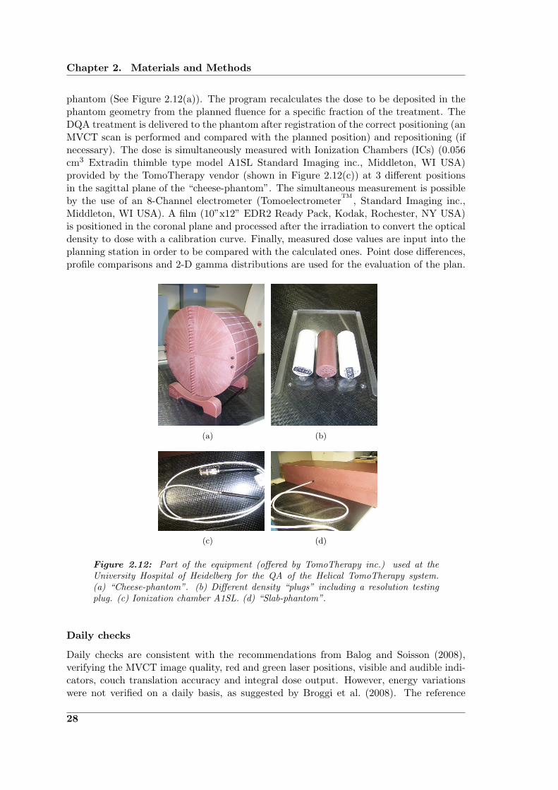
Chapter 2. Materials and Methods
phantom (See Figure 2.12(a)). The program recalculates the dose to be deposited in thephantom geometry from the planned fluence for a specific fraction of the treatment. TheDQA treatment is delivered to the phantom after registration of the correct positioning (anMVCT scan is performed and compared with the planned position) and repositioning (ifnecessary). The dose is simultaneously measured with Ionization Chambers (ICs) (0.056cm3 Extradin thimble type model A1SL Standard Imaging inc., Middleton, WI USA)provided by the TomoTherapy vendor (shown in Figure 2.12(c)) at 3 different positionsin the sagittal plane of the “cheese-phantom”. The simultaneous measurement is possibleby the use of an 8-Channel electrometer (Tomoelectrometer
TM, Standard Imaging inc.,
Middleton, WI USA). A film (10”x12” EDR2 Ready Pack, Kodak, Rochester, NY USA)is positioned in the coronal plane and processed after the irradiation to convert the opticaldensity to dose with a calibration curve. Finally, measured dose values are input into theplanning station in order to be compared with the calculated ones. Point dose differences,profile comparisons and 2-D gamma distributions are used for the evaluation of the plan.
(a) (b)
(c) (d)
Figure 2.12: Part of the equipment (offered by TomoTherapy inc.) used at theUniversity Hospital of Heidelberg for the QA of the Helical TomoTherapy system.(a) “Cheese-phantom”. (b) Different density “plugs” including a resolution testingplug. (c) Ionization chamber A1SL. (d) “Slab-phantom”.
Daily checks
Daily checks are consistent with the recommendations from Balog and Soisson (2008),verifying the MVCT image quality, red and green laser positions, visible and audible indi-cators, couch translation accuracy and integral dose output. However, energy variationswere not verified on a daily basis, as suggested by Broggi et al. (2008). The reference
28

2.4. Application to TomoTherapy: dose delivery verification tool
plan alluded in test D3, was performed for QA purposes using the CT scan images ofthe cheese-phantom as “patient”. In this geometry, a simulated cylindrical target volumein the upper part of the phantom and an organ at risk in the central part of it (alsocylindrical) were delineated and then, a treatment plan was calculated.
Weekly checks
Test W2 is performed using the slab-phantom (Figure 2.12(d)) and two ICs measuringsimultaneously at depths of 10 and 20 cm. W4 is performed using the set-up shown inFigure 2.12(b). The resolution is tested visually by identifying the last “resolvable” rowof the resolution plug. The fiducial marks in the acrylic base are used to check the spatialaccuracy of the imaging system and the position of the virtual isocenter. The test W5,developed by Balog et al. (2006), lasts only 100 s and allows the testing of many of theunique features of the system. Analyzing the charge collected (every 100 ms) by twoICs positioned inside the cheese-phantom (at 5 mm from the center and 14 cm radiallyoutwards in the most distal hole from the couch), parameters like the gantry period, couchoffset, integral dose, energy and table velocity, can be tested. This test requires the use ofthe vendor supplied QA equipment.
Monthly checks
Many of the monthly tests recommended by Balog and Soisson (2008) such as imagequality check, the D20/D10 test and the measurement of the couch speed among othersare performed on a more regular basis (weekly) at the University Hospital of Heidelberg.Tests M1, M2 and M3 are performed using EDR2 films and the slab phantom for differentMLC, gantry and couch configurations. These procedures and the evaluation software(TomoTherapy Film Analyzer) are provided with the system. Test M4 also uses the slabphantom and an EDR2 film. M5, M6 and M7 are performed using the same patient planand the cheese-phantom. Test M8 is performed using an IC, which is positioned directlyat the isocenter in a phantom that only provides the necessary build-up material. The ICremains static, measuring the collected charge every 100 ms, while the gantry constantlyrotates around it with a period of 60 s for a time lapse of 30 min. The MLC leaves areopen during the complete process.
Semestral checks
Semestral checks are basically the ones described by Balog and Soisson (2008) to betested on an annual basis. These checks include most of the commissioning tests andshould reproduce the respective values. The water tank measurements were not strictlyperformed in 6-month intervals, but every time the target was replaced.
Yearly checks
The correct functioning of all security systems and the vertical accuracy of the table weretested on a yearly basis.
As many of the dosimetric tests included in the QA program are proposed and evalu-ated by the system itself and/or require specific equipment supplied by the same company,the implementation of a supplemental QA procedure, is proposed. This procedure, based
29

Chapter 2. Materials and Methods
on the dose calculation method presented in Section 2.3, would serve to test the overallperformance of the system and the effect of individual parameter variations (e.g., out-put, gantry speed, and table velocity) within the treatment. Once the patient treatmentsinograms are available, it can also be used as a patient specific delivery verification test.
Table 2.2: Schedule of the QA program for the TomoTherapy unit at the UniversityHospital of Heidelberg (Kai Schubert, private communication).
Patient specific checks
P1 Patient DQA:Film, coronal 2-D dose distribution (Gamma index<1, 3%/3mm)IC measurements (3 simultaneous points)target volume(s) and organ(s) at risk (±3%)
Daily checks
D1 Visible and audible indicators (working)D2 MVCT air scan (no artifacts)D3 Reference plan:
MU constancy (±1%)Table position before and after the plan (±1mm)Laser position (±1mm)
Weekly checks
W1 Lasers:Red (movable) relative laser position (±1mm)Green (static) absolute laser position (±1mm)
W2 Absolute dosimetry:Dose at 10 cm depth in a virtual-water phantom (±1%)Dose at 20 cm depth in a virtual-water phantom (±1%)D20/D10 (±1%)
W3 Reference plan:IC measurement, high dose (±2%)IC measurement, low dose (±2%)Film, coronal 2-D dose distribution (Gamma index<1, 2%/2mm)Film, longitudinal profile (optic agreement)
W4 MVCT image quality:Transverse distance between markers (±1mm)Longitudinal distance between markers (±1mm)Virtual isocenter (±1mm)Hounsfield Units, low, medium and high densityResolution (1 mm)
W5 Dynamic test:Energy (±1%)
Continued on next page...
30

2.4. Application to TomoTherapy: dose delivery verification tool
Table 2.2 – Continued from previous page
Gantry period (±0.2s)Table velocity, FWHM of lateral profile (±1mm)Table offset (±1mm)Integral dose (±2%)
Monthly checks
M1 Virtual isocenter offset in x,y and z (±1mm)M2 MLC center/gantry isocenterM3 Central axis-Y axis misalignmentM4 Longitudinal field, uniformity and size (Gamma index<1, 1%/1mm)M5 MVCT dose (<2 cGy)M6 Patient plan:
IC measurement, high dose (±3%)IC measurement, medium dose (±3%)IC measurement, low dose (±3%)Film, coronal 2-D dose distribution (Gamma index<1, 3%/3mm)
M7 Patient plan with interruption, compared with the non-interrupted:IC measurement, high dose (±2%)IC measurement, medium dose (±2%)IC measurement, low dose (±2%)Film, coronal 2-D dose distribution (Gamma index<1, 1%/1mm)
M8 Rotational test:Output constancy (±2%)Output angular dependence (±2%)
Semestral checks
S1 Transverse profile at different gantry angles (Gamma index<1, 2%/2mm)S2 Hounsfield UnitsS3 Water tank static IC measurements (after target replacement):
PDDsLongitudinal and transverse profiles at different depths
Yearly checks
Y1 Security systems (working)Y2 Table vertical position accuracy (±1mm)
31

Chapter 2. Materials and Methods
2.4.4 Dose verification using the small-field model as a supplementalquality assurance test
The beam model presented in Section 2.3 has been validated to ensure that it can ac-curately reproduce dose distributions in water using small fields. Therefore, it has beenimplemented as the central engine of the calculation algorithm used for the TomoTherapydose verification tool.
Using this verification tool, three-dimensional dose distributions were obtained in ahomogeneous (water equivalent) virtual cylindrical phantom, coaxially aligned with thegantry rotation axis. A schematic representation of this phantom, indicating the mainevaluation planes (where the results were obtained and visualized), is shown in Figure2.13. The axis of the cylindrical phantom has a length of 20 cm and a radius is of 10 cm.The calculation voxels were defined to be of 1x1x1 mm3.
Figure 2.13: Virtual cylindrical phantom and main evaluation planes.
Static Mode
The input data required to implement the model into the dose calculation tool was col-lected using, in principle, the same methods as described in Section 2.3. Only a fewmodifications regarding the reference conditions were introduced. The reference field, inthe TomoTherapy case, corresponded to a 40x5 cm2 field defined at 85 cm from the source.The weights of the spectrum used for the determination of the poly-energetic PBK wereobtained by fitting the calculated PDD to the one measured for this new reference condi-tion. As mentioned before, the absence of a flattening filter makes the mean energy changeat off-axis positions to be less than 5% (Jeraj et al., 2004). Therefore, no correction forlateral spectral changes was applied.
As the table sunk (∼1-2 mm) while it was moved from the virtual isocenter (where theslit-collimator device was positioned) to real isocenter (70 cm apart in the longitudinaldirection), it was not possible to determine the exact position of the source with respectto the Central AXis (CAX) (i.e., the slit was not perfectly aligned with it). Therefore, it
32

2.4. Application to TomoTherapy: dose delivery verification tool
could only be assumed that the source was centered. The validity of this assumption canbe evaluated by the comparison between measured and calculated penumbras.
Planar dose distributions were obtained according to 2.3.3, although some small dif-ferences from the method described previously had to be considered. The first one is thefact that, in the case of TomoTherapy, the “envelope profile” obtained does not correctfor the horn-effect produced by the flattening filter. On the contrary, it accounts for thecharacteristic cone shaped distribution of the fluence (see Figure 2.11(a)), due to the ab-sence of a flattening filter. The second one is that, in this case, the leakage contributionto the final dose calculation has been included as an additive component to the 2-D dosedistributions obtained. The leakage was taken into account by a cross-profile measured inthe X direction with all the leaves of the MLC closed and the Y -jaws set to their maximumopening (relative to the maximum dose when all leaves are open and the jaws project a 5cm field at the isocenter plane). To obtain the 2-D distribution needed for the planar dosecalculations, the profile was replicated and weighted by the envelope distribution in theperpendicular direction. The specific shape of the collimators and other (second order)effects related with the MLC hardware have not been explicitly modeled. These include:the tongue&groove effects and the fact that the leaves are not perfectly back-focused tothe source, thus, the fluence at a certain position under a leaf is influenced by the state(open/closed) of neighboring leaves.
Dynamic Mode
Three dynamic modes of the system can be identified. These are:
• Topographic: the couch moves longitudinally while the gantry angle is fixed duringthe complete beam-on time.
• Rotational: the couch is fixed while the gantry continuously rotates around it untilthe procedure is finished.
• Helical: both couch and gantry move simultaneously throughout the treatment.
All patients are treated in helical mode. The first two modes are used only for QApurposes. The verification tool presented here can calculate dose distributions for any ofthese modes including, of course, the static mode.
The final dose distributions were obtained as follows:
1. Beamlet calculation: The dose delivered to the virtual cylindrical phantom (centeredin the longitudinal direction) was calculated using the static mode of the system(with the CAX perpendicular to the couch plane), for each one of the leaves openedindividually and for each one of the three possible openings of the Y -jaws (the fieldwidth in the Y direction is fixed during the treatment to either 1, 2.5 or 5 cmprojected to the isocenter plane). Each “beamlet” distribution was stored for lateruse. After this step, the model is no longer needed.
2. Input of basic treatment parameters: The algorithm requires, as a first step forthe determination of the integral dose (after the beamlet distributions have beendetermined), the input of the main treatment parameters. These include: (i) theopening of the Y -jaws (1, 2.5 or 5 cm), (ii) the number of projections used in acomplete rotation of the gantry (the default is 51, as this is the value used by the
33
Chapter 2. Materials and Methods
TPS to plan patient treatments), (iii) the gantry period (between 10 and 60 s) and(iv) the displacement of the couch after a 360◦ gantry rotation. If the number ofprojections per gantry rotation is fixed to 51 and the jaw setting is given, the onlyextra treatment parameter needed is the pitch (see Equation 2.11). Typical pitchvalues used in patient treatments range from 0.25 to 0.5 (Kissick et al., 2005).
3. Initial conditions: Before starting the calculation process, the initial longitudinalposition of the center of the phantom and the gantry angle need to be set.
4. Sinogram “filtering”: The sinogram, described in Section 2.4.2, contains all the infor-mation related to the modulation of the beam (performed in the transverse direction,perpendicular to the patient movement). The optimized modulation patterns foreach patient treatment obtained by the TPS, are subject to some modifications be-fore the data is transferred to the delivery system. Even though currently the patientspecific sinograms cannot be directly extracted from the TPS and implemented intothe calculation tool. Here, the dynamic effects that introduce modifications into thecalculated sinograms (and the corrections that account for them) to be implementedas part of a patient specific QA procedure, are pointed out. The first sinogram fil-tering, done projection by projection, is related to the latency of the MLC leaves. Ittakes approximately 10 ms to open/close each leaf. The opening time of each leaf ina projection is obtained by multiplying the opening fraction by the gantry period,and dividing it by the number of projections per rotation. If any of the leaves is pro-grammed to be open in a specific projection for a period of time equal or less than 20ms, the leaf is set to be closed during the complete projection time. Also dependingon the projection time and latency, the opening fractions of the leaves are recalcu-lated by a linear transform that accounts for the effective opening with respect to theprogrammed time. A transform function for a specific projection time is obtainedby fitting straight lines to measured values of the effective opening time with respectto the programmed one (this behavior is similar within leaves). This process is donefor different projection times, between 200 ms (although the minimum projectiontime allowed for patient treatments is of 294 ms, corresponding to 51 projectionsper gantry rotation with a rotation period of 15 s) and 1000 ms (where the linearrelation between programmed and effective opening time has a slope of ∼1). If theprojection time does not coincide with the ones used to obtain the transforms, thetransform is obtained by simple linear interpolation (if the projection time is largerthan 1000 ms, then the transform obtained for 1000 ms is used). This process hasbeen described by Balog et al. (2003).
5. Projection dose: The dose deposited in the phantom by the delivery of a singleprojection (Dp) is calculated in the following way: The pre-calculated beamlets(bY,ln) corresponding to each leaf (ln) and to the nominal opening of the Y -jaws (Y )are weighted by their opening time (Ot,p,ln) and summed. Then, the distribution isrotated (interpolation is needed) and shifted; according to the gantry angle (θp) andthe longitudinal position of the phantom (yp), both corresponding to the projection(p). i.e.,
Dp(x, y, z) =64∑ln=0
Ot,p,ln · bY,ln(x cos(θp) + z sin(θp), y − yp,−x sin(θp) + z cos(θp)),
(2.12)
34

2.4. Application to TomoTherapy: dose delivery verification tool
where the coordinates (x, y, z) refer to the coordinate system shown in Figure 2.9(a).The opening time Ot,p,ln, angle θp and phantom position yp are determined as
Ot,p,ln = Of,p,ln ·T
pr, (2.13)
θp = θi +(p
pr· 360◦
)mod 360◦ (2.14)
andyp = yi +
p
pr· yr, (2.15)
respectively, where x mod y returns the least common residue of the division x/y1,Of,p,ln is the fraction of the projection time that the leaf ln remains open for theprojection p, T is the gantry period, pr is the number of projections per gantryrotation, θi is the initial gantry angle, yi is the initial longitudinal position of thecenter of the phantom and yr is the couch displacement per gantry rotation. Therotation angle is defined clockwise starting from the Z direction.
6. Integral dose: The final dose distribution (Df ) is obtained by superposing the dis-tributions calculated for each projection of the treatment as
Df (x, y, z) =pf∑p=0
Dp(x, y, z), (2.16)
where pf is the total number of projections of the (filtered) sinogram.
2.4.5 Test of the tool
The dose verification tool was evaluated in the static and dynamic modes by comparingmeasured and calculated values.
Static tests
Using the static mode of the system, measurements were carried out by a diode detector ina water tank at 15 mm depth with a SSD of 85 cm. The tests consisted in the comparisonof measured and calculated OFs and dose profiles for different collimator configurations.
Output factors were determined for a fixed Y -jaws opening (5 cm at the isocenter)varying the field size in the perpendicular direction (MLC) from 1.25 to 40 cm definedat the surface. Only symmetric openings were considered. The performance of the toolregarding the modeling of dose distributions in the plane perpendicular to the CAX (par-allel to the couch plane) was tested in the X and Y directions for different rectangularfields and also for a more complex MLC pattern (where every other pair of leaves was setto be open).
Figure 2.14 shows the sinogram used for the measurement of OFs and planar doseprofiles for different field openings in the X direction. It has, initially, 30 projectionswhere all the leaves remain close (to provide sufficient time for the stabilization of the
1Weisstein, Eric W. “Modulus”. From MathWorld–A Wolfram Web Resource.http://mathworld.wolfram.com/Modulus.html.
35

Chapter 2. Materials and Methods
beam output before starting the measurements). Then, every 10 projections, an additionalamount of leaves were open (symmetrically) until all of them were open (during the timecorresponding to 10 projections, starting from the projection number 160). A differentprojection time was used for each set of measurements, as the scanning of the profilesrequired a longer time than the measurement of OFs.
60
50
40
30
20
10
0
15010050060
50
40
30
20
10
0150100500
Leaf
num
ber
Projection number
Figure 2.14: Sinogram used to measure the OFs and the rectangular dose profiles.
Dynamic tests
The three dynamic modes (topographic, rotational and helical) of the system were testedfor a simple MLC configuration, in which the four central leaves (projecting a field widthof 2.5 cm at the isocenter) were set to be open during the complete irradiation time.The Y -jaws opening was fixed to 2.5 cm (projected to the isocenter). The measurementswere performed using the cheese-phantom (see Figure 2.12(a)) and a film positioned inthe coronal plane that divided the cheese-phantom in two equal halves. Transverse andlongitudinal profiles were compared. The treatment parameters (described in Section2.4.4) used for each treatment mode are displayed in Table 2.3.
Table 2.3: Parameters used for the evaluation of the dose verification tool in thedifferent dynamic modes. (∗)Even though the gantry remains fixed in the topographicprocedure, it is necessary to input the values for every parameter in order to assignthe absolute projection time and couch velocity.
Parameter Unit Topographic(∗) Rotational Helical
θi◦ 0 0 0
yi cm -5 0 -5
T s 10 10 10
pr - 10 10 10
yr cm 1 1 1
pf - 100 20 100
36
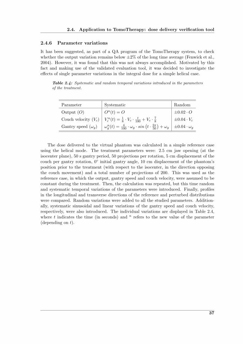
2.4. Application to TomoTherapy: dose delivery verification tool
2.4.6 Parameter variations
It has been suggested, as part of a QA program of the TomoTherapy system, to checkwhether the output variation remains below ±2% of the long time average (Fenwick et al.,2004). However, it was found that this was not always accomplished. Motivated by thisfact and making use of the validated evaluation tool, it was decided to investigate theeffects of single parameter variations in the integral dose for a simple helical case.
Table 2.4: Systematic and random temporal variations introduced in the parametersof the treatment.
Parameter Systematic Random
Output (O) On(t) = O ±0.02 ·OCouch velocity (Vc) V n
c (t) = 18 · Vc ·
t100 + Vc · 7
8 ±0.04 · VcGantry speed (ωg) ωng (t) = 4
100 · ωg · sin(t · 2π
50
)+ ωg ±0.04 · ωg
The dose delivered to the virtual phantom was calculated in a simple reference caseusing the helical mode. The treatment parameters were: 2.5 cm jaw opening (at theisocenter plane), 50 s gantry period, 50 projections per rotation, 5 cm displacement of thecouch per gantry rotation, 0◦ initial gantry angle, 10 cm displacement of the phantom’sposition prior to the treatment (with respect to the isocenter, in the direction opposingthe couch movement) and a total number of projections of 200. This was used as thereference case, in which the output, gantry speed and couch velocity, were assumed to beconstant during the treatment. Then, the calculation was repeated, but this time randomand systematic temporal variations of the parameters were introduced. Finally, profilesin the longitudinal and transverse directions of the reference and perturbed distributionswere compared. Random variations were added to all the studied parameters. Addition-ally, systematic sinusoidal and linear variations of the gantry speed and couch velocity,respectively, were also introduced. The individual variations are displayed in Table 2.4,where t indicates the time (in seconds) and n refers to the new value of the parameter(depending on t).
37


“We can have facts without thinking but we cannothave thinking without facts.”
John Dewey (1859-1952)
3Results
The results of this work are presented in this chapter. They are divided into two parts:First, the establishment and validation of the dose calculation engine and second, the useof this model in a dose verification tool for TomoTherapy. The concepts and specific meth-ods and materials employed for the determination of these results have been previouslydescribed in Chapter 2. Their discussion and interpretation will be presented separatelyin Chapter 4.
3.1 Beam model
The developed dose calculation algorithm aims at modeling accurately the dose depositionin homogeneous media for narrow beams. For this purpose, a kernel-based method (PBK),which allows handling the non-CPE conditions within narrow fields by explicitly modelingthe energy transport of the secondary particles, was used. The other effect that has beentaken into account in the modeling of small fields is the partial blocking of the source.For this, the effect of an experimentally determined extended source was included into themodeling of the fluence distribution. This extended source distribution not only includesthe focal spot, but also the head scatter contributions.
In this section, the results of each step in the determination of the extended sourceare presented, followed by the determination of the poly-energetic PBK based on pre-calculated mono-energetic DDKs. Then, the results of the validation tests for the modelare given. The tests have included the comparison between measured and calculatedplanar dose profiles and OFs for quadratic and circular fields of different sizes. Most ofthe results presented in the first part of this chapter can also be found in Caprile andHartmann (2009).
3.1.1 Extended source
As described in Section 2.3.1, the extended source is defined as the projection of all pri-mary photons and head scatter contributions into a common plane. This two-dimensional
39
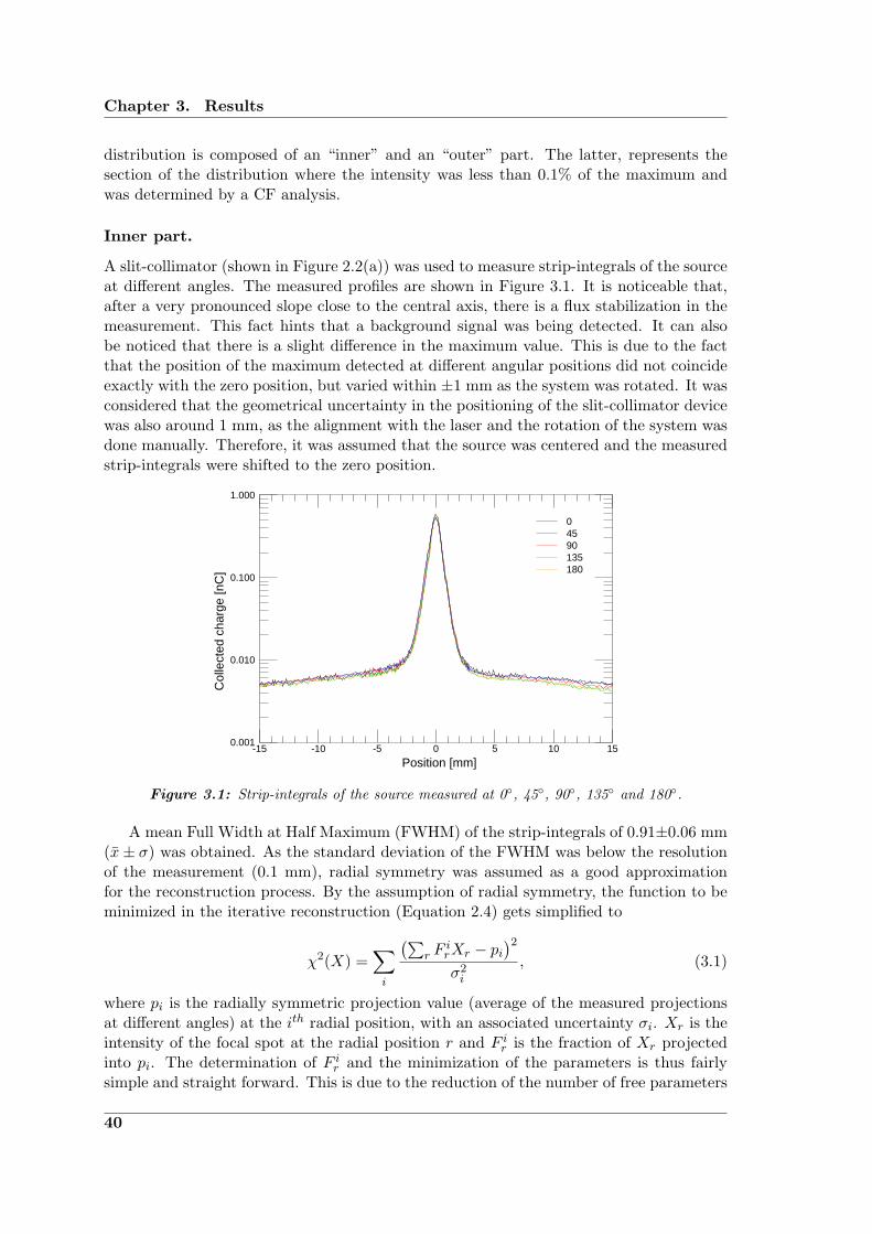
Chapter 3. Results
distribution is composed of an “inner” and an “outer” part. The latter, represents thesection of the distribution where the intensity was less than 0.1% of the maximum andwas determined by a CF analysis.
Inner part.
A slit-collimator (shown in Figure 2.2(a)) was used to measure strip-integrals of the sourceat different angles. The measured profiles are shown in Figure 3.1. It is noticeable that,after a very pronounced slope close to the central axis, there is a flux stabilization in themeasurement. This fact hints that a background signal was being detected. It can alsobe noticed that there is a slight difference in the maximum value. This is due to the factthat the position of the maximum detected at different angular positions did not coincideexactly with the zero position, but varied within ±1 mm as the system was rotated. It wasconsidered that the geometrical uncertainty in the positioning of the slit-collimator devicewas also around 1 mm, as the alignment with the laser and the rotation of the system wasdone manually. Therefore, it was assumed that the source was centered and the measuredstrip-integrals were shifted to the zero position.
1.000
0.100
0.010
0.001151050-5-10-15
Col
lect
ed c
harg
e [n
C]
Position [mm]
18013590450
Figure 3.1: Strip-integrals of the source measured at 0◦, 45◦, 90◦, 135◦ and 180◦.
A mean Full Width at Half Maximum (FWHM) of the strip-integrals of 0.91±0.06 mm(x± σ) was obtained. As the standard deviation of the FWHM was below the resolutionof the measurement (0.1 mm), radial symmetry was assumed as a good approximationfor the reconstruction process. By the assumption of radial symmetry, the function to beminimized in the iterative reconstruction (Equation 2.4) gets simplified to
χ2(X) =∑i
(∑r F
irXr − pi
)2σ2i
, (3.1)
where pi is the radially symmetric projection value (average of the measured projectionsat different angles) at the ith radial position, with an associated uncertainty σi. Xr is theintensity of the focal spot at the radial position r and F ir is the fraction of Xr projectedinto pi. The determination of F ir and the minimization of the parameters is thus fairlysimple and straight forward. This is due to the reduction of the number of free parameters
40
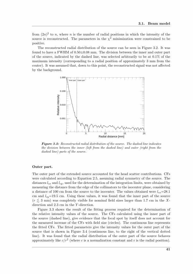
3.1. Beam model
from (2n)2 to n, where n is the number of radial positions in which the intensity of thesource is reconstructed. The parameters in the χ2 minimization were constrained to bepositive.
The reconstructed radial distribution of the source can be seen in Figure 3.2. It wasfound to have a FWHM of 0.50±0.08 mm. The division between the inner and outer partof the source, indicated by the dashed line, was selected arbitrarily to be at 0.1% of themaximum intensity (corresponding to a radial position of approximately 3 mm from thecenter). It was assumed that, down to this point, the reconstructed signal was not affectedby the background.
1.000
0.100
0.010
0.001
20151050
Outer partInner part
Radial distance [mm]
Rel
ativ
e in
tens
ity
Figure 3.2: Reconstructed radial distribution of the source. The dashed line indicatesthe division between the inner (left from the dashed line) and outer (right from thedashed line) parts of the source.
Outer part.
The outer part of the extended source accounted for the head scatter contributions. CFswere calculated according to Equation 2.5, assuming radial symmetry of the source. Thedistances lcx and lcy, used for the determination of the integration limits, were obtained bymeasuring the distance from the edge of the collimators to the isocenter plane, consideringa distance of 100 cm from the source to the isocenter. The values obtained were lcx=28.1cm and lcy=19.5 cm. Using these values, it was found that the inner part of the source(r . 3 mm) was completely visible for nominal field sizes larger than 1.7 cm in the X-direction and 2.3 cm in the Y -direction.
Figure 3.3 shows the result of the fitting process required for the determination ofthe relative intensity values of the source. The CFs calculated using the inner part ofthe source (dashed line), give evidence that the focal spot by itself does not account forthe measured increase of the CFs with field size (circles). The continuous line representsthe fitted CFs. The fitted parameters give the intensity values for the outer part of thesource that is shown in Figure 3.4 (continuous line, to the right of the vertical dottedline). It was found that the radial distribution of the outer part of the source behavesapproximately like c/r2 (where c is a normalization constant and r is the radial position).
41
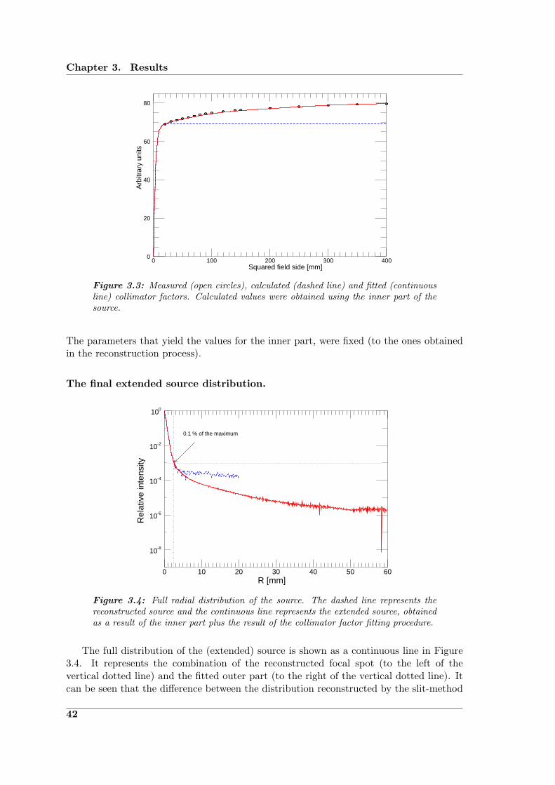
Chapter 3. Results
80
60
40
20
04003002001000
Squared field side [mm]
Arb
itrar
y un
its
Figure 3.3: Measured (open circles), calculated (dashed line) and fitted (continuousline) collimator factors. Calculated values were obtained using the inner part of thesource.
The parameters that yield the values for the inner part, were fixed (to the ones obtainedin the reconstruction process).
The final extended source distribution.
100
10-2
10-4
10-6
10-8
6050403020100
0.1 % of the maximum
Rel
ativ
e in
tens
ity
R [mm]
Figure 3.4: Full radial distribution of the source. The dashed line represents thereconstructed source and the continuous line represents the extended source, obtainedas a result of the inner part plus the result of the collimator factor fitting procedure.
The full distribution of the (extended) source is shown as a continuous line in Figure3.4. It represents the combination of the reconstructed focal spot (to the left of thevertical dotted line) and the fitted outer part (to the right of the vertical dotted line). Itcan be seen that the difference between the distribution reconstructed by the slit-method
42
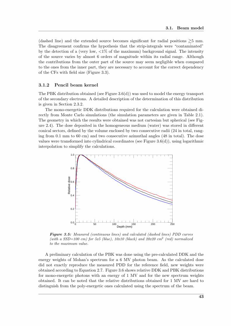
3.1. Beam model
(dashed line) and the extended source becomes significant for radial positions &5 mm.The disagreement confirms the hypothesis that the strip-integrals were “contaminated”by the detection of a (very low, <1% of the maximum) background signal. The intensityof the source varies by almost 6 orders of magnitude within its radial range. Althoughthe contributions from the outer part of the source may seem negligible when comparedto the ones from the inner part, they are necessary to account for the correct dependencyof the CFs with field size (Figure 3.3).
3.1.2 Pencil beam kernel
The PBK distribution obtained (see Figure 3.6(d)) was used to model the energy transportof the secondary electrons. A detailed description of the determination of this distributionis given in Section 2.3.2.
The mono-energetic DDK distributions required for the calculation were obtained di-rectly from Monte Carlo simulations (the simulation parameters are given in Table 2.1).The geometry in which the results were obtained was not cartesian but spherical (see Fig-ure 2.4). The dose deposited in the homogeneous medium (water) was stored in differentconical sectors, defined by the volume enclosed by two consecutive radii (24 in total, rang-ing from 0.1 mm to 60 cm) and two consecutive azimuthal angles (48 in total). The dosevalues were transformed into cylindrical coordinates (see Figure 3.6(d)), using logarithmicinterpolation to simplify the calculations.
1.0
0.8
0.6
0.4
0.2
0.0250200150100500
Rel
ativ
e do
se
Depth (mm)
Figure 3.5: Measured (continuous lines) and calculated (dashed lines) PDD curves(with a SSD=100 cm) for 5x5 (blue), 10x10 (black) and 20x20 cm2 (red) normalizedto the maximum value.
A preliminary calculation of the PBK was done using the pre-calculated DDK and theenergy weights of Mohan’s spectrum for a 6 MV photon beam. As the calculated dosedid not exactly reproduce the measured PDD for the reference field, new weights wereobtained according to Equation 2.7. Figure 3.6 shows relative DDK and PBK distributionsfor mono-energetic photons with an energy of 1 MV and for the new spectrum weightsobtained. It can be noted that the relative distributions obtained for 1 MV are hard todistinguish from the poly-energetic ones calculated using the spectrum of the beam.
43
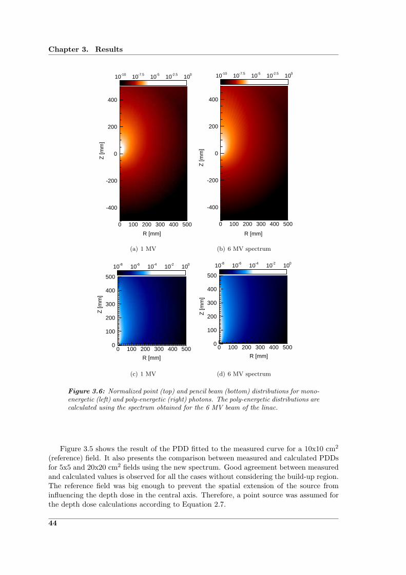
Chapter 3. Results
400
200
0
-200
-400
5004003002001000
10-10 10-7.5 10-5 10-2.5 100
Z [m
m]
R [mm]
(a) 1 MV
400
200
0
-200
-400
5004003002001000
10-10 10-7.5 10-5 10-2.5 100
R [mm]
Z [m
m]
(b) 6 MV spectrum
500
400
300
200
100
05004003002001000
10-8 10-6 10-4 10-2 100
Z [m
m]
R [mm]
(c) 1 MV
500
400
300
200
100
05004003002001000
10-8 10-6 10-4 10-2 100
Z [m
m]
R [mm]
(d) 6 MV spectrum
Figure 3.6: Normalized point (top) and pencil beam (bottom) distributions for mono-energetic (left) and poly-energetic (right) photons. The poly-energetic distributions arecalculated using the spectrum obtained for the 6 MV beam of the linac.
Figure 3.5 shows the result of the PDD fitted to the measured curve for a 10x10 cm2
(reference) field. It also presents the comparison between measured and calculated PDDsfor 5x5 and 20x20 cm2 fields using the new spectrum. Good agreement between measuredand calculated values is observed for all the cases without considering the build-up region.The reference field was big enough to prevent the spatial extension of the source frominfluencing the depth dose in the central axis. Therefore, a point source was assumed forthe depth dose calculations according to Equation 2.7.
44

3.1. Beam model
3.1.3 Validation tests
The model was validated for a 6 MV photon beam using a variety of field sizes, includingcircular and quadratic fields. Since the stereotactic collimators (formed by tungsten cylin-ders of 10 cm in height with different internal radii) were positioned at a SCD of 59 cm(distance from the source to the distal edge of the collimator), the circular fields projectedat the measurement plane had a diameter dm = 1.72 · dc (where dc is the collimator di-ameter). Conversely, the field of view of the detector projected to the source plane had adiameter ds = 1.93 · dc. Therefore, the inner part of the source (r . 3 mm) was uncoveredfrom the detector’s point of view for collimators with dc & 3 mm, as the detector waspositioned at 1015 mm from the source.
To test the performance of the model in a homogeneous medium (as the aim was touse it for dose delivery verification in a homogeneous phantom), calculated OFs and doseprofiles (at 15 mm depth with a SSD of 100 cm) were compared with measured values inthe same conditions. These measurements were obtained using a diode in a water tank.
Output factors
Two methods to determine the OFs for the circular fields have been used: (i) directdiode measurements in the central axis and (ii) indirect determination by measurementof the relative 2-D distribution and use of a parallel plate chamber (see Section 2.3.4).Both results are shown in Figure 3.7(a) as circles and triangles, respectively. It can beseen that both methods agree well with each other, although some small (non-systematic)differences can be found. The continuous line represents the calculated OFs for the sameconditions using the extended source in a calculation grid of 0.1x0.1 mm2. They show aremarkable agreement with the diode measurements. The dashed line shows the effect ofconsidering a point-like source in the determination of the dose. This calculation indicatesthe strong effect of the integration of the PBK within the field opening for the small fields,shaping the curve with the characteristic shoulder. It is also evidence of the importanceof considering the spatial extension of the source to accurately model the OFs for smallfields. This is particularly evident for the collimators with smaller apertures (dc =1, 2 and3 mm), which partially block the inner part of the source. For these cases, the difference inoutput between the point-source calculations and the measured values reaches 22.4% (forthe smallest collimator aperture) with respect to the normalization value (correspondingto the collimator with dc=20 mm). The difference in the same case, but considering theextension of the source, is 1.4%. The calculated OFs agreed with the (diode) measuredvalues within ±2% of the normalization value (except for the value corresponding to thecollimator with dc=2 mm, for which the difference was of 2.07%).
Figure 3.7(b) shows the measured and calculated OFs for the quadratic fields. Con-sidering the extension of the fields (maximum field size of 40x40 cm2) and the fact thatthe uncertainty in the field size compared with the nominal value is on the order of 1mm, a coarser calculation grid (of 1x1 mm2) was used in order to reduce the calculationtime. The same trend already shown for the circular fields is observed here, demonstrat-ing that the approximation of the source as a point (considering the phantom scatter bythe integration of the PBK contribution within the field) is not sufficient to model theincrease of dose deposited on the central axis with increasing field size (see dashed line).The OFs calculated using the extended source appear to be in good agreement with thevalues measured with the diode. The discrepancies observed for the first three measure-
45

Chapter 3. Results
ments (corresponding to quadratic field sides of 5, 10 and 20 mm in length) should bejudged considering that the corresponding (visible) section of the extended source has avery steep slope, and thus, a small deviation in the field size (the uncertainties associatedwith the field size are of the order of 1 mm) leads to an important variation in output.
1.0
0.8
0.6
0.4
0.2
0.020151050
OF
Collimator diameter [mm]
(a)
0
1.2
1.0
0.8
0.6
0.4
0.2
0.04003002001000
Field side [mm]
OF
(b)
Figure 3.7: Output factors: measured with a diode (open circles), measured witha combination of diode and parallel plate chamber (open triangles), calculated usingthe extended source (continuous lines) and using a point source (dashed lines). (a)Circular fields. (b) Quadratic fields.
In general, the combination of PBK and extended source showed to be appropriate tomodel OFs from very small field sizes (the smallest field size evaluated corresponded to acircular field with dm = 1.7 mm at the measurement plane) to the biggest available (40x40cm2 at the isocenter).
46

3.1. Beam model
Dose profiles
The final test of the model consisted in the evaluation of its performance modeling lateraldose profiles (Figure 3.8), with particular interest in the penumbra (i.e., the region betweenthe 90% and 10% dose points on the beam profile) of the small circular fields.
100
90
80
70
60
50
40
30
20
10
03020100−10−20−30
Rel
ativ
e do
se
Position [mm]
(a)
100
90
80
70
60
50
40
30
20
10
0150100500−50−100−150
Position [mm]
Rel
ativ
e do
se
(b)
Figure 3.8: Relative dose profiles measured (continuous lines) and calculated (dashedlines) for different field sizes. The dotted lines represent 10 ∗ γ (gamma index value,γ < 1 : pass, γ > 1 : fail) for each profile. (a) Circular fields. (b) Quadratic fields.
Figure 3.8(a) shows the comparison between measured and calculated dose profiles forthe fields generated by the cylindrical collimators. The dotted lines represent the gammaindex value (amplified by 10 for better visualization) with individual acceptance criteriaof 2% dose difference and 0.5 mm DTA. This evaluation indicates that the calculationshave passed the test in all the cases shown in the figure (corresponding to collimators with
47

Chapter 3. Results
dc =1, 2, 10 and 20 mm). The good agreement indicates that the criteria could have beenfurther tightened. The only regions presenting minor discrepancies (slight overestimationof the dose with respect to the measured values) corresponded to the central part of theprofile for the collimator with dc = 2 mm, and to the tails of the profile measured for thecollimator with dc = 20 mm.
Although the capacity of the pencil beam method to accurately model dose distribu-tions for homogeneous media under conditions of CPE has already been widely studiedand confirmed (Mohan et al., 1986; Bourland and Chaney, 1992; Ahnesjo et al., 1992;Storchi and Woudstra, 1996; Bortfeld, 2006), the modeled and measured lateral profilesfor quadratic fields covering the complete range of possible field sizes were compared inorder to have a complete validation of the model. Figure 3.8(b) shows the result of thiscomparison for (quadratic) field sides of s =1, 5, 10 and 20 cm length measured in theY -direction.
For the quadratic fields the gamma index test (dotted lines) has been used again withthe same dose difference criterion as for the evaluation of the circular fields (2%), butthe DTA criterion has been changed to a value of 2 mm (considering that the calculationgrid used for these calculations was of 1x1 mm2 and that the uncertainty in the field sizewas higher than for the circular fields). The calculations presented here lie within theseacceptance criteria in every case, the agreement is particularly good in the penumbraregion. Small differences can be seen for the fields with s =10 and 20 cm on the leftside of the central axis, in the region close to the “horns” of the profile. There, thecalculated distributions slightly overestimated the measured dose at the correspondingoff-axis position. It can be noted that the measured profiles for these field sizes are notperfectly symmetric with respect to the central axis of the beam. As the measured fieldspresented a systematic asymmetry with respect to the CAX of approximately 1 mm, thecalculations were shifted for better comparison. A justification and analysis of this shiftis given in Section 4.1.4.
3.2 TomoTherapy dose verification tool
In this section the results related to the integration of the model into a dose verificationtool applicable to TomoTherapy delivered dose distributions and to the performance ofthe tool itself are presented. First, the input distributions necessary to apply the model tothis system are presented. Then, the results of the evaluation of the model in its static anddynamic modes are shown. Finally, the comparison between a reference helical treatmentcalculation and the result of the same treatment, modified by temporal variations of thecouch and gantry positions and of the beam output, is presented.
3.2.1 Model components
The components needed to implement the developed dose calculation model (described inSection 2.3) into a TomoTherapy dose calculation tool are the following: the determinationof the extended source and the poly-energetic PBK, and the obtainment of the profilesused to correct the calculated planar dose distributions for the lateral fluence variation(envelope profile) and for the leakage contributions (see Section 2.4.4).
48

3.2. TomoTherapy dose verification tool
Source distribution
The extended source distribution of the TomoTherapy treatment beam (6 MV) was de-termined using the same combination of methods as in the validation of the model (slit-method and CF fitting, see Section 2.3.1).
1.000
0.100
0.010
0.00120100-10-20
Position [mm]
Col
lect
ed c
harg
e [n
C/s
]
90450
(a)
100
10-1
10-2
10-3
10-4
10-5
10-6
20151050
Outerpartpart
Inner
Radial distance [mm]R
elat
ive
inte
nsity
(b)
Figure 3.9: Slit-method TomoTherapy source reconstruction. (a) Strip-integral ofthe source measured at 0◦, 45◦ and 90◦. (b) Reconstructed distribution.
Figure 3.9(a) shows the unnormalized strip-integrals of the source measured at differentangular positions, with the detector positioned at a distance of approximately 65 cm fromthe source. The jaws and MLC openings were set to provide a nominal field size of 10x5cm2 at the isocenter plane. The 0◦ measurement corresponds to a scan of the source in thetransverse direction (X axis). It can be seen that the shape of the measured distributions,with a FWHM of 1.37±0.02 mm (x±σ), are virtually indistinguishable from the maximumvalue down to ∼1% of the maximum intensity (corresponding to a off-axis distance of ∼3mm). Therefore, radial symmetry of the focal spot was assumed for the reconstruction.The radial distribution of the reconstructed source is shown in Figure 3.9(b). It has aFWHM of 0.72±0.05 mm. The dashed line shows the division between the inner andouter parts of the source (at 0.1% of the maximum intensity), this point corresponds to aradial distance of approximately 3.4 mm.
As the nature of the discrepancies in the strip-integrals, corresponding to intensityvalues lower tan 1% of the maximum, was not certain (most probably due to an unde-termined amount of scatter radiation coming not directly from the source), it was onlypossible to assume radial symmetry also for the outer part. The outer part was obtainedfollowing the procedure described in Section 2.3.1 and according to this, it was foundthat the inner part of the source was completely visible from the isocenter point for fieldopenings greater than 1.67 cm in the X direction and 2.80 cm in the Y direction. Figure3.10(b) shows the result of the least-squares fitting process, for which the reconstructeddistribution (and a c/r2 distribution for the missing values) was used as a first guess. Thefitted parameters produced a very good agreement between the measured (interpolated)and modeled CFs. However, it can be seen in Figure 3.10(a) that the fitted parametersare subject to some artifacts of the fitting process (related to interpolation issues andthe non-negativity constraint), which are accentuated due to the fact that, after the firstthree evaluated fields, the increase of CF with increasing field size is almost negligible.
49
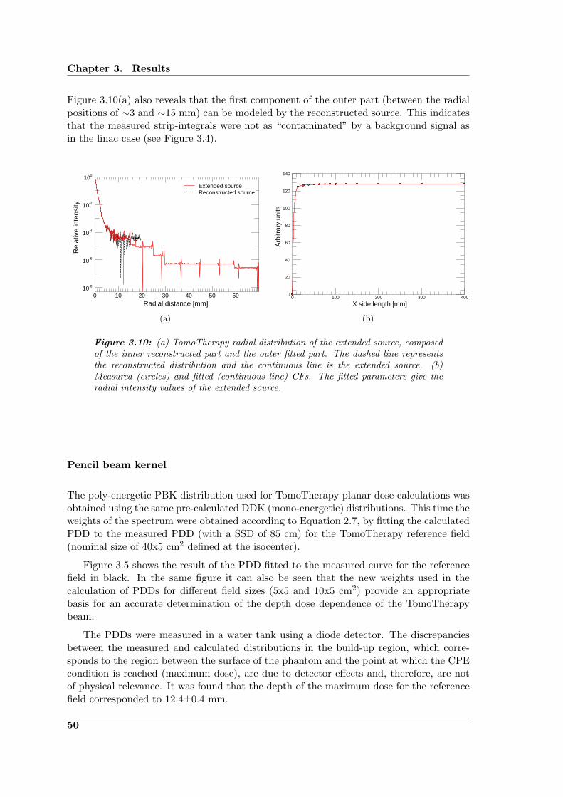
Chapter 3. Results
Figure 3.10(a) also reveals that the first component of the outer part (between the radialpositions of ∼3 and ∼15 mm) can be modeled by the reconstructed source. This indicatesthat the measured strip-integrals were not as “contaminated” by a background signal asin the linac case (see Figure 3.4).
100
10-2
10-4
10-6
10-8
6050403020100
Radial distance [mm]
Rel
ativ
e in
tens
ity
Reconstructed sourceExtended source
(a)
140
120
100
80
60
40
20
04003002001000
X side length [mm]
Arb
itrar
y un
its
(b)
Figure 3.10: (a) TomoTherapy radial distribution of the extended source, composedof the inner reconstructed part and the outer fitted part. The dashed line representsthe reconstructed distribution and the continuous line is the extended source. (b)Measured (circles) and fitted (continuous line) CFs. The fitted parameters give theradial intensity values of the extended source.
Pencil beam kernel
The poly-energetic PBK distribution used for TomoTherapy planar dose calculations wasobtained using the same pre-calculated DDK (mono-energetic) distributions. This time theweights of the spectrum were obtained according to Equation 2.7, by fitting the calculatedPDD to the measured PDD (with a SSD of 85 cm) for the TomoTherapy reference field(nominal size of 40x5 cm2 defined at the isocenter).
Figure 3.5 shows the result of the PDD fitted to the measured curve for the referencefield in black. In the same figure it can also be seen that the new weights used in thecalculation of PDDs for different field sizes (5x5 and 10x5 cm2) provide an appropriatebasis for an accurate determination of the depth dose dependence of the TomoTherapybeam.
The PDDs were measured in a water tank using a diode detector. The discrepanciesbetween the measured and calculated distributions in the build-up region, which corre-sponds to the region between the surface of the phantom and the point at which the CPEcondition is reached (maximum dose), are due to detector effects and, therefore, are notof physical relevance. It was found that the depth of the maximum dose for the referencefield corresponded to 12.4±0.4 mm.
50

3.2. TomoTherapy dose verification tool
100
80
60
40
20
0120100806040200
PD
D [%
]
Depth [mm]
Figure 3.11: Measured (continuous lines) and calculated (dashed lines) TomoTher-apy PDD curves (with SSD=85 cm) for 5x5 (blue), 10x5 (red) and 40x5 cm2 (black)normalized to the maximum value.
Envelope and leakage
Figure 3.12(a) shows transverse profiles measured with a diode detector at 15 mm depthin a water tank with a SSD of 85 cm. The fields were defined by the maximum Y -jawsopening and a variable number of open MLC leaves, ranging from 0 to 64 (symmetric withrespect to the CAX). Two important characteristics of the beam can be identified fromthis figure: (i) the cone shape of the beam, product of the unmodulated photon fluence(absence of flattening filter); and (ii) the low increase of the relative beam output withincreasing field size, again related to the absence of a flattening filter and the subsequentreduction of head scatter contributions. For the calculation process described in Section2.3.3, the profile measured for the biggest field size of 40x5 cm2 was used as the radiallysymmetric envelope profile (after a deconvolution with the PBK at 15 mm depth to accountfor the relative fluence variation instead of dose variation).
A zoom into Figure 3.12(a) is presented in Figure 3.12(b) to visualize better the cross-profile measured when all the MLC leaves were set to be closed (relative to the dose in thecentral axis measured for the largest field available). It can be seen that the TomoTherapysystem produces very low additional dose contributions (below 0.4%) outside the radiationfield, which are due to intra- or inter-leaf leakage (in most of the distribution was of evenless than 0.3%, with a mean of 0.14%). This is due to the design of the tungsten MLCleaves (10 cm long) coupled with an effective tongue and groove design. Even thoughsmall, the leakage contributions were considered in the calculations (see Section 2.4.4).The transmission through the Y -jaws was negligible, as in this direction the jaws arecomposed of up to 23 cm of tungsten.
These two distributions are the last components necessary to implement the dosecalculation engine into the dose verification tool for TomoTherapy (as the source andPBK were already characterized).
51

Chapter 3. Results
100
80
60
40
20
02001000-100-200
Rel
ativ
e do
se [%
]
Position [mm]
(a)
0.5
0.4
0.3
0.2
0.1
0.02001000-100-200
Leak
age
[%]
Position [mm]
(b)
Figure 3.12: Helical TomoTherapy cross-profiles. (a) Transverse profiles for differ-ent MLC openings. (b) MLC leakage.
3.2.2 Test results
The capability of the dose verification tool to reproduce dose distributions delivered by theTomoTherapy system to a homogeneous phantom was evaluated using each of its modes(static, topographic, rotational and helical). In this section, the comparisons betweenmeasured and calculated beam profiles and OFs are presented.
Static mode
The measurements performed to test the model were done in a water tank using a diodein the plane parallel to the couch with the linac pointing straight downwards. The dosewas calculated for the same conditions, using a calculation grid of 1x1 mm2.
20
15
10
5
150100500-50-100-150Position [mm]
Arb
itrar
y un
its
Figure 3.13: TomoTherapy static calculation: X profiles. Measured (continuousline) and calculated (dashed line) profiles in the X direction for different MLC open-ings.
52

3.2. TomoTherapy dose verification tool
Figure 3.13 shows the comparison of measured and calculated profiles in theX directionfor different MLC openings, the Y -jaws projected a field size of 5 cm to the isocenterplane for every evaluated field. Consistent with the validation results, the profiles arefound to be in good agreement with the values measured with a diode. All studied casespass the acceptance criteria of 2%/2mm globally defined (with respect to the maximumdose). However, small differences were observed. For example, the maximum dose wasunderestimated by the calculation method in the smaller field size evaluated (1.25 cm atthe isocenter in the X direction). Another mild disagreement is found in the “tail” of thebiggest field shown (corresponding to a nominal field of 20 cm in the X direction), forwhich the measured dose was also slightly underestimated.
The modeling of OFs (shown as the solid line in Figure 3.14) shows a very good agree-ment with the measured values. The differences remain under ±2% of the normalizationvalue (corresponding to a nominal field size of 10x5 cm2). The maximum deviation was-1.98%, corresponding to the smallest field size evaluated of only 1.25 cm in the X direc-tion. The differences between modeled and measured OFs for the rest of the evaluatedfields remain below 1%.
1.0
0.8
0.6
0.4
0.2
0.04003002001000
OF
X side length [mm]
Figure 3.14: TomoTherapy static calculation: Output factors. Measured (circles)and calculated (continuous line) OFs.
Even though subtle, as the CF and OF distributions (Figures 3.10(b) and 3.14, respec-tively) exhibit almost no increase for field sizes larger than 5x5 cm2, the OFs show a morepronounced increase due to the spread of the dose in water (phantom scatter), accountedfor by the PBK.
Planar dose profiles using the static mode of the system were evaluated in both direc-tions (X and Y ) for simple MLC configurations (symmetric rectangular fields). Figure3.15 shows the performance of the tool in the modeling of dose profiles in the main axisof the plane perpendicular to the CAX. The relative intensity of the profiles is displayedon a logarithmic scale. From this figure, it can be seen that the shape of the penumbrasand the tails of the profile in the different directions are not the same. Although somedeviations between the modeled and measured profiles (within the acceptance criteria)can be observed, the tool is able to predict correctly the shape of the different penumbrasof the field in the complete scanned range (down to ∼0.5% of the maximum).
53

Chapter 3. Results
Figure 3.15: TomoTherapy static calculation: X v/s Y profiles. Measured (continu-ous lines) and calculated (dashed lines) profiles in the X (blue) and Y (red) directionsof a 5x5 cm2 field.
1.0
0.8
0.6
0.4
0.2
0.02001000-100-200
Position [mm]
Rel
ativ
e do
se
Figure 3.16: TomoTherapy static calculation: Cross-profile of an MLC dose pattern.Measured (continuous line) and calculated (dashed line) profile. The Y -jaws are attheir maximum opening and the MLC has every other pair of leaves open.
Good agreement (below 2%/2mm) between the measured and calculated profile canalso be seen in Figure 3.16, indicating that the tool is also well suited to predict dose dis-tributions in asymmetric configurations for different MLC patterns. The maximum doseunder each pair of open leaves was predicted very accurately, however, some small differ-ences were observed for positions where the beam was blocked by the closed leaves (mini-mum dose). There, the dose was slightly overestimated by the calculation tool (∼1.5%).Also, it can be seen that certain penumbra regions within the pattern (specially on theright side with respect to the CAX) appear to be “shifted” from the measured positions(with a maximum shift corresponding to ∼2 mm). It is not clear if these discrepancies area result of detector effects, interpolation and voxel averaging issues or inaccuracies related
54
3.2. TomoTherapy dose verification tool
to the MLC position and shape.
Dynamic mode
The dose verification tool was tested in the three dynamic modes (topographic, rotationaland helical) for a simple MLC/jaws configuration (projecting a square field size to theisocenter plane of 2.5x2.5 cm2) that was fixed during the complete treatment time. Thedifferent treatment parameters used for the evaluation of each mode can be seen in Table2.3. The integral dose was calculated in the virtual cylindrical phantom (Figure 2.13) anddelivered to the cheese-phantom (Figure 2.12(a)) using the same parameters and the sameMLC configuration. The dose was measured with a film positioned at the coronal planeof the cheese phantom.
Figure 3.17 shows the results of the dynamic test. All the evaluated cases show goodagreement (better than 2%/2mm) with the measured profiles in the longitudinal direction.The distributions were normalized to the dose at the center of the phantom. It can be seenthat the measured profiles are not smooth and flat in the “plateau” region (Figures 3.17(a)and 3.17(g)), but show some discrepancies from the calculated results. This indicates thatthere is a temporal variation of one or more of the treatment parameters within theirradiation procedure. Although less evident (because of the narrower plateau region),this effect is also observed in the rotational case (Figure 3.17(d)). The second and thirdcolumns of the figure show the calculated relative 2-D dose distributions in the transverseand sagittal planes of the virtual phantom for the three dynamic modes. In Figures3.17(b) and 3.17(c), some artifacts related with interpolation and grid size of the beamletcalculation can be seen.
3.2.3 Parameter variations
As seen in Figure 3.18, variations in the output of the beam (obtained in the staticmode) were in general within the recommended ±2% (see Section 2.4.6) of the long termaverage. However, this was not always the case (see yellow line), thus, the impact ofsimilar variations (and additional ones) in the integral dose of a simple helical case wasinvestigated. The variations included systematic and random components.
In Section 2.4.6 the specific variations introduced to the beam output, the speed of thegantry and the couch velocity are given. These can also be visualized on the left side ofFigure 3.19. On the right side of the figure, the result of introducing these variations canbe seen. The reference helical distribution was calculated using the treatment parametersdescribed in Section 2.4.6. The output, couch velocity and gantry speed were constantduring the complete irradiation procedure. The distributions were compared (referenceprofiles are shown as continuous lines and the variation results as dashed lines) in thecoronal plane of the virtual cylindrical phantom (shown in Figure 2.13) on the X and Yaxis. Figure 3.19(b) shows that a random variation of ±2% in the output of the beamthroughout the treatment does not introduce any considerable influence to its final out-come. Similar results are obtained by considering an uncertainty in the table velocity of4% of the nominal value and a constant acceleration (of 0.001 mm/s2). In this case thediscrepancies on the longitudinal axis are greater than for the output variation, never-theless, they still remain within ±2% of the maximum dose. The gantry speed variation,corresponding to a systematic sinusoidal variation (reducing the velocity by an amplitudeof 4% of the nominal value as the linac moves upwards and increasing as the linac moves
55

Chapter 3. Results
100
80
60
40
20
06040200-20-40-60
Rel
ativ
e do
se
Position [mm]
(a)
100
80
60
40
20
0Z
X
(b)
100
80
60
40
20
0Z
Y
(c)
100
80
60
40
20
06040200-20-40-60
Rel
ativ
e do
se
Position [mm]
(d)
100
80
60
40
20
0
X
Z
(e)
100
80
60
40
20
0Z
Y
(f)
100
80
60
40
20
06040200-20-40-60
Rel
ativ
e do
se
Position [mm]
(g)
100
80
60
40
20
0Z
X
(h)
100
80
60
40
20
0Z
Y
(i)
Figure 3.17: TomoTherapy dynamic calculation: Longitudinal (first row), rotational(second row) and helical (third row) modes. The first column (from left to right)shows the comparison between the measured (black lines) and calculated (red lines)relative dose profiles in the longitudinal direction of the coronal plane at the cylindricalphantom. The gamma value (blue lines) with acceptance criteria of 2%/2mm is shownamplified by 10 for better visualization. Dashed lines indicate the limit of acceptancefor the gamma index. The second column shows the distributions calculated in thetransverse plane of the virtual cylindrical phantom and the third column shows thedistributions obtained for the sagittal plane.
56
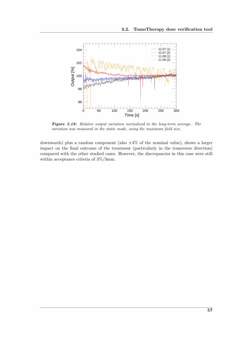
3.2. TomoTherapy dose verification tool
104
102
100
98
96
300250200150100500Time [s]
Out
put [
%]
11.08 (2)11.08 (1)12.07 (2)12.07 (1)
Figure 3.18: Relative output variation normalized to the long-term average. Thevariation was measured in the static mode, using the maximum field size.
downwards) plus a random component (also ±4% of the nominal value), shows a largerimpact on the final outcome of the treatment (particularly in the transverse direction)compared with the other studied cases. However, the discrepancies in this case were stillwithin acceptance criteria of 3%/3mm.
57

Chapter 3. Results
104
102
100
98
96
200150100500
Bea
m o
utpu
t [%
]
Time [s]
(a)
100
80
60
40
20
0100500-50-100
Position [mm]
Rel
ativ
e do
se(b)
1.2
1.1
1.0
0.9
0.8200150100500
Time [s]
Cou
ch v
eloc
ity [m
m/s
]
(c)
100
80
60
40
20
0100500-50-100
Rel
ativ
e do
se
Position [mm]
(d)
0.022
0.021
0.020
0.019
0.018200150100500
Gan
try
rota
tiona
l spe
ed [1
/s]
Time [s]
(e)
100
80
60
40
20
100500-50-100
Rel
ativ
e do
se
Position [mm]
(f)
Figure 3.19: Effect of random and systematic parameter variations on a test heli-cal case. Left: variation introduced. Right: Comparison between calculated coronalprofiles X (red) and Y (blue), with (dashed line) and without (continuous line) theinclusion of the variation.
58
“Research is the process of going up alleys to see ifthey are blind.”
Marston Bates (1906-1974)
4Discussion
The rationale and methodology employed in the development of a dose verification tool forTomoTherapy were presented in Chapter 2. The main parameters of the dose calculationmodel have been determined and used to produce dose distributions delivered by theTomoTherapy system (using its different modes) in a homogeneous phantom. Additionally,variations in some of the delivery parameters were introduced. The integral dose obtainedunder these circumstances was compared with a reference distribution. These results werepresented in the previous chapter. In this chapter, these results are analyzed in theircontext; addressing issues related to the establishment and implementation of the dosecalculation model. A critical evaluation of the performance and usability of the proposeddose verification tool is also presented.
4.1 First part: The beam model
The dose calculation model presented in this study is a PBK-based algorithm that includesa detailed description of the extended source (focal spot + outer part, see Section 2.3.1).The determination of the poly-energetic PBK is based on pre-calculated mono-energeticDDK distributions obtained from Monte Carlo simulations (see Section 2.3.2).
The validation of this algorithm was performed using the 6 MV beam of a SiemensPrimus linac for circular and quadratic fields. The focus of the model was set to accuratelyreproduce OFs and dose profiles for small fields, i.e., fields with sizes in the order of twotimes the range of the secondary electrons in the medium, or smaller. Considering thatfor a 6 MV clinical beam the forward range of the electrons corresponds approximatelyto 1.5 cm, CPE conditions will be present in the center of fields with diameters largerthan 3 cm. This limit can be tightened to about 1.5 cm when considering, as discussedby Das et al. (2008), not the forward but rather the lateral range of the secondary par-ticles (corresponding to approximately half of the forward range) as the key parameterdefining the CPE conditions. The validation results, shown in Section 3.1.3, demonstratethat the model presented in this work provides an adequate approach to determine dosedistributions in water for both small and large fields.
59

Chapter 4. Discussion
Within this section, an analysis of the extended source and of the methods used toreconstruct it, is presented. In particular, the effects observed in the measured strip-integrals, used for the focal spot reconstruction, are analyzed. With the source fullycharacterized, the individual influences of the source and the PBK on the final dose calcu-lations (penumbra and output) for different collimator configurations are compared. Then,the results of the validation tests are discussed in detail, in order to assess the advantagesoffered by the approach presented here and also the current limitations of the model.
4.1.1 On the slit-method and the determination of the source
When performing slit-collimator measurements with the unshielded detector, it becameclear that a part of the radiation detected by the diode was due to background radiation.Therefore, a shielding was added to the diode, particularly effective in the lateral direction(perpendicular to the slit).
Figure 4.1(a) shows measured strip-integrals of the source using two different shieldingmaterials for the diode. The first attempt to reduce the background signal was madeusing a brass shielding, which resulted in an immediate reduction of the background. Thisconfirmed the assumption that the signal was enhanced by radiation coming from partsother than the slit and served as a motivation to further reduce this effect by implementinga more effective shield made of tungsten. Even though the new shielding reduced thebackground signal even more (∼4.5% with respect to the brass shielding), a small detectorflux (of less than 1% compared to the maximum) was still observed at distances of 5mm and larger. This flux presented a constant contribution to the measured slit. Asit turned out that the associated (calculated) increase of the output factor free in airwas still too large compared with the measured CFs, it became clear that it was notpossible to reconstruct the complete source distribution (for distances larger than 5 mmfrom the source center) using the data of the slit measurement. The small discrepanciesobserved in the central part of the strip-integrals do not correspond to the backgroundeffect, but rather to the different SCDs used. The measurement taken the brass shieldingwas performed at an SCD that was 20 cm larger than the one used for tungsten, thus, theresolution of the slit at the source plane (projection of the slit-collimator opening) wascoarser for a larger SCD.
To further understand the nature of the background signal detected by the diode, a slit-integral was measured varying the openings of the secondary collimators. It was found thatthe intensity of the background signal was field size dependent: increasing with increasingfield size (though the effect was more subtle than the variations observed for the changein shielding material). As the field size was reduced, it could be noticed, that at certainscanning positions, the measured signal did not correspond to radiation coming from thesource plane: the slit was blocked by the collimators. Figure 4.1(b) shows strip-integralsmeasured in the Y direction for the same experimental setup, but with a varying openingof the secondary collimators. It can be seen that the reproducibility of the measurementsin the central part of the distribution is remarkably good. Also, as mentioned before, areduction in the signal at the wings of the distribution is observed for the smaller fieldopening. It is interesting to see how the point where the collimator structure begins isclearly defined, as the collimator starts “eclipsing” the source plane from the detector’spoint of view. The distance from the source to the effective edge of the Y -jaws was lcy=19.5cm measured (obtained by manually measuring the distance from the collimator to theisocenter position and assuming an SAD of 100 cm), thus, a nominal field side of 6 cm
60

4.1. First part: The beam model
100
10
1
1086420-2-4-6-8-10
4.5%
Position [mm]
Rel
ativ
e in
tens
ity
(a)
100
10
1
1086420-2-4-6-8-10
5.8 mm6.1 mm
Position [mm]
Rel
ativ
e in
tens
ity
(b)
Figure 4.1: Effects observed in the measurement of strip-integrals of the source. (a)Strip-integrals of the source measured for a nominal field size of 10x10 cm2 in the Ydirection using different shielding materials for the diode: brass (black circles) andtungsten (red circles). (b) Strip-integrals of the source measured in the Y directionusing the tungsten shielding for different nominal field sizes: 6x6 cm2 (black circles)and 10x10 cm2 (red circles.)
length (symmetric with respect to the central axis) in the Y direction, requires a collimatoropening of 1.17 cm (5.85 mm to each side). It was found (as indicated in Figure 4.1(b))that the collimator was blocking the slit from the starting position of the measurement(-10 mm) to a position of -6.1 mm from the central axis. The next blocking occurred at+5.8 mm (in very good agreement with the calculations). These openings, projected tothe isocenter plane correspond to 3.13 and 2.97 cm respectively. As shown in Table 4.1,this analysis was later confirmed by the measurement of field sizes in the Y direction,showing a systematic CAX deviation of ∼1 mm and also a systematic deviation from thenominal size corresponding to ∼1 mm. The same analysis in the perpendicular directionwas not performed because it was impossible to clearly resolve the exact point where thecollimators first blocked the slit (it was a rather smooth change, perhaps associated withincrease in the background scatter, interleaf leakage and transmission contributions). Thisis an example of an alternative use of the slit-method, which serves not only to reconstructthe source shape but also to study the fine details of the radiation field.
Besides the background effects, the radial variations of the source were also investigatedby obtaining strip-integrals at different angles (see Figure 3.1). The first finding from thisanalysis was that the maximum value was not exactly the same for different angularpositions, furthermore, it did not always correspond to the central axis position but wasslightly deviated (within ±1 mm). This indicates either that the source was not centered orthat the device was not positioned correctly. As the stability of the slit measuring device(after manual rotation) and the precision of the alignment of the slit with the centralaxis (also done manually) yield an estimated uncertainty of the position of the detectorof ∼1 mm, it was not possible to untangle these possibilities. Hence, it was assumedthat the source was aligned with the central axis and the measured strip-integrals were
61

Chapter 4. Discussion
shifted in order to establish a coincidence between the maximum and the zero position.As the standard deviation of the FWHMs of the distributions was less than 0.1 mm,radial symmetry of the source was assumed as a good approximation for the focal spotreconstruction process.
Focal spots (inner part of the source) of medical linear accelerators have been deter-mined in the past using different methods, such as slit-collimators (Munro et al., 1988),deconvolution techniques (Treuer et al., 1993) and the analysis of OFs (Zhu et al., 1995).As stated before, the slit-collimator method was selected for being the most direct andquantitative among them. Jaffray et al. (1993) studied the focal spots of several linacs(including Varian, Siemens and AECL) for different energies, obtaining focal spots withFWHMs in the range of 0.6 to 2.9 mm with deviations from rotational symmetry varyingfrom 0 to 1.3 mm. In the work presented here, a symmetric focal spot, with a FWHM of0.50±0.08 mm was obtained. This result is similar to that found by Jaffray et al. (1993)for a Siemens KD-2 linac using the 6 MV beam (major axis: 0.7 mm, minor axis: 0.5mm), as shown in Figure 3.2.
(a) (b)
Figure 4.2: Comparison of focal spots. Dashed lines divide the plane in regionsof 1x1 mm2. The contour lines indicate the 10%, 30%, 50%, 70% and 90% of themaximum intensity. (a) Focal spot of a a Siemens KD-2 linac using the 6 MV beamfrom Jaffray et al. (1993). (b) Focal spot of a Siemens Primus linac for the 6 MVbeam, obtained for the validation of the beam model using the slit-method.
Due to the aforementioned limitations of the slit-method to accurately determine thedistribution of the source at off-axis positions, the outer part of the extended source wasdetermined using the same concept as in the numerical single source model described byChui et al. (2003). This method obtains the (symmetric) shape of the radiation source byfitting the head scatter factors (or CFs) of quadratic fields of different sizes. Therefore,the accuracy on the determination of the source distribution using this method dependsdirectly on the accuracy of the CFs. It was assumed that the measured CFs using thediode detector (with an appropriate build-up cup) were reliable (i.e., sufficiently accurate)for field sizes larger than 2x2 cm2 and, thus, were used for the determination of the outerpart of the source (shown in Figure 3.4). Although this method presents a much simplerapproach to determine the radial distribution of the source, its usefulness to obtain theinner part is limited by its resolution (it would require a huge amount of CFs measuredfor very small fields to map the steep slope of the inner part of the source) and accuracy(large uncertainties are associated with small field measurements).
62

4.1. First part: The beam model
The method to construct a radial distribution of the source by the combination ofthe slit-method for the focal spot and the CFs analysis for the outer part, provides asufficiently accurate and flexible tool to calculate dose distributions and OFs in water fora broad range of field sizes (from a few millimeters up to 40 cm), as shown in Section3.1.3.
4.1.2 On the pencil beam determination
Since the introduction of the concept of pencil beam kernels for photon dose calculations,many ways of obtaining the PBK have been used. These include: deconvolution tech-niques (Chui and Mohan, 1988), experimental methods (Ceberg et al., 1996; Storchi andWoudstra, 1996), Monte Carlo based techniques (Mohan and Chui, 1987; Ahnesjo andTrepp, 1991; Bourland and Chaney, 1992) and analytic/parametric approaches (Ahnesjoet al., 1992; Bortfeld et al., 1993; Nyholm et al., 2006). As stated in Section 2.3.2, aMonte Carlo based technique was used to obtain the final PBK from pre-calculated pointkernel distributions (appropriately weighted to fit a measured PDD curve in a broad beamconfiguration). Once the mono-energetic point kernels (DDKs) are obtained, getting theweights of the spectrum (from the fitting procedure) is conceptually a straight forwardprocedure. This simplicity provides the approach with the flexibility of reusing the samepoint kernels in the calculation of PBKs for any beam (if the nominal energy is includedin the calculated DDKs).
In Figure 3.5, an example of how the Monte Carlo based PBK accurately reproducesthe depth dependence of the absorbed dose in the CAX for quadratic fields in the rangeof 5x5 cm2 to 20x20 cm2 for a 6 MV beam of a Siemens Primus linac can be seen.
Although the concept of obtaining the poly-energetic PBK is clear, the method is notexempt of implementation issues. The most prominent are: (i) the interpolation of theDDK distributions (which originally come in a spherical geometry, not very practical forplanar dose calculations) and (ii) finding the correct weights of the spectrum by means ofthe minimization.
The raw DDK data coming directly out of the Monte Carlo simulations needed someprocessing before being ready to be used for the determination of the PBK and as the con-volution kernel distribution in the final dose calculation (here, interpolation into cartesiancoordinates is needed for the use of FFT). As these distributions are symmetric aroundthe polar angle (see Figure 2.4), they were transformed into cylindrical coordinates (afterassigning the dose of each voxel to an effective radius and an azimuthal angle). Thisprocess required interpolation of the data. It was found that a bilinear interpolation on alogarithmic base was an appropriate method. It was also found that the result of the finalPBK was strongly influenced by the value of the central bin in the DDK distributions,because close to the origin the slopes of the distributions are very steep. Therefore, theinterpolation/rebinning process required a careful consideration of these effects. Theseissues have been discussed by Eklof et al. (1990); Rathee et al. (1993) and Ahnesjo andAspradakis (1999).
From the pre-calculated DDK distributions for 24 energy bins (between 250 KeV and6 MeV), 24 mono-energetic depth dose profiles were calculated. These were used in theleast-squares minimization process to obtain the spectrum weights (see Equation 2.7). Itwas found that the dependence of the final dose on the weights was not very strong (i.e.,many different combinations yield the same or at least a very similar solution), therefore,some constraints were set in order to force the parameters (energy weights) to vary only
63

Chapter 4. Discussion
little with respect to the first guess (Mohan’s spectrum for 6 MV, Mohan et al. 1985).It was also necessary to constrain the parameters so they could only take positive values(Scholz et al., 2003), as otherwise the solution would have not been physically valid.
4.1.3 On the individual effects of the source and pencil beam kernel
The convolution-based method to calculate planar dose distributions has been presentedin Section 2.3.3. Here, the individual characteristics of the convolution kernels (source andpencil beam) that shape the penumbra of the field and are responsible for the increase ofthe output with the increase of field size are analyzed.
The individual influence of these effects on the OF is presented in Figure 3.7. It canbe seen that none of the effects by themselves would account for the precise increase ofoutput with field size, but the combination of both yield a very good agreement withthe measurements for both circular and quadratic configurations. In the latter, greaterdiscrepancies in the small field section of the curve were observed due to the uncertaintiesassociated to the field size and the increase of the calculation grid size from 0.1x0.1 (forthe circular fields) to 1x1 mm2. It can be noticed that the PBK by itself (point sourceapproximation) already provides the basic shape of the curve by reducing the output as thefield sizes decrease and steepening the curve as we enter the regime of non-CPE conditionswithin the field (for s .2 cm or dc .10 mm). However, it cannot model the “eclipsing” ofpart of the radiation source, which is particularly important for the very small fields, wheresections of the inner part of the source (steepest part of the extended source distribution)are being blocked. Even though the outer part of the source does not have an importantinfluence on the OFs for the circular fields, it is very important for the large quadraticfields, as it accounts for the head scatter contribution (projected into the source plane)that represents an important part of the total increase in output for larger field sizes.The major contribution to the head scatter comes from the flattening filter. This can bededuced comparing the increase of CFs with field size for the linac (Figure 3.3) with theone for the TomoTherapy system (Figure 3.10(b)), which does not use flattening filter.
Figure 4.3 shows the individual 2-D convolution functions, scaled source and PBK atthe measurement depth as used in the determination of the planar dose distributions forthe two field configurations used in the validation of the model (circular fields, shaped byadd-on cylindrical collimators and quadratic fields shaped by the Y -jaws and the MLC ofthe linac). The field penumbra modeled by the different effects (individually and combined)is also included. The effects on the cylindrical configuration will be analyzed first.
It can be seen from Figures 4.3(a), 4.3(b) and 4.3(c) that the source and pencil beamkernel distributions are very similar in shape and intensity. However, the scaled sourcedisplays a steeper slope than the PBK at the measurement depth. As the circular fieldswere defined by single cylindrical collimators located at a fixed distance from the source,the presented model produces radially symmetric distributions. This is due to the addi-tional facts that the PBK is defined to be radially symmetric (see Section 2.3.2) and thatthe reconstructed source was assumed to be centered and radially symmetric (see Sections3.1.1 and 4.1.1). This symmetry was confirmed by diode measurements performed in theX and Y directions, for which the discrepancies in the penumbra were within ±0.1 mm,indicating that the assumptions on the source were appropriate. Figure 4.3(d) shows thepenumbra of a field of 8.6 mm in diameter (corresponding to the collimator with a diameterdc=5 mm), measured (red) and modeled (black): by the combined effect (dot-dashed line)and considering the source (dashed line) and PBK (dotted line) effects individually. The
64

4.1. First part: The beam model
20 10 0
-10
-20
2010
0-1
0-2
0
20 10 0
-10
-20
2010
0-1
0-2
0
0-1
-2-3
-4-5
X [m
m]
Y [mm]
(a)
20 10 0
-10
-20
2010
0-1
0-2
0
20 10 0
-10
-20
2010
0-1
0-2
0
0-1
-2-3
-4-5
Y [mm]
X [m
m]
(b)
100
10-1
10-2
10-3
10-4
10-5
10-6
2010
0-1
0-2
0
Relative intensity
Y [m
m]
(c)
1.0
0.8
0.6
0.4
0.2
0.0
86
42
0
Relative intensity
Y [m
m]
(d)
200
100 0
-100
-200
200
100 0
-100
-200
200
100
0-1
00-2
00
200
100
0-1
00-2
00
0-2
-4-6
-8
X [m
m]
Y [mm]
(e)
200
100
0-1
00-2
00
200
100
0-1
00-2
00
200
100 0
-100
-200
200
100 0
-100
-200
0-2
-4-6
X [m
m]
Y [mm]
(f)
100
10-2
10-4
10-6
10-8
200
100
0-1
00-2
00
Relative intensity
Y [m
m]
(g)
1.0
0.8
0.6
0.4
0.2
0.0
5040
3020
100
Relative intensity
Y [m
m]
(h)
Fig
ure
4.3
:T
heex
tend
edso
urce
(con
side
ring
the
rela
tive
dist
ance
sbe
twee
nth
eco
llim
ator
s,th
eso
urce
and
the
mea
sure
men
tpl
ane)
,th
eus
edpo
ly-e
nerg
etic
PB
K(a
tth
em
easu
rem
ent
dept
h)an
dth
eir
indi
vidu
aleff
ects
onth
eca
lcul
atio
nof
plan
ardo
sedi
stri
buti
ons
for
the
circ
ular
(top
)an
dqu
adra
tic
(bot
tom
)fie
lds.
From
left
tori
ght:
(a,e
)sc
aled
2-D
sour
cedi
stri
buti
ons
at15
mm
.(b
,f)
2-D
PB
Kdi
stri
buti
ons.
(c,g
)C
ross
-pro
files
ofth
eso
urce
(con
tinu
ous
lines
)an
dP
BK
(das
hed
lines
)di
stri
buti
ons.
(d,h
)R
elat
ive
dose
profi
les
mea
sure
d(c
onti
nuou
sre
dlin
es)
for
afie
ldpe
rfor
med
byth
eci
rcul
arco
llim
ator
wit
hd
c=
5m
m(d
)an
dfo
ra
quad
rati
cfie
ldof
side
leng
ths=
5cm
(h).
The
non-
solid
lines
indi
cate
the
calc
ulat
edpr
ofile
sfo
ra
poin
tso
urce
(onl
yth
eP
BK
effec
tw
asco
nsid
ered
,do
tted
lines
),fr
ee-i
n-ai
r(o
nly
the
sour
ceeff
ect
was
cons
ider
ed,
dash
edlin
es)
and
usin
gth
eex
tend
edso
urce
(bot
heff
ects
wer
eco
nsid
ered
,do
t-da
shed
lines
).
65

Chapter 4. Discussion
combination of both effects can almost perfectly model the drop of the dose at the edgeof the field. Although the point source approximation reproduces the penumbra of thefield slightly better than the case in which no energy transport of the secondary electronsis considered, neither of the individual effects by themselves can model the penumbra ofthe small circular fields as good as the combination of them. It should be noticed thatthe point source approximation would be sufficient to fulfill an acceptance criteria for thedose circular dose profiles of 2%/0.5 mm (as they are normalized to the maximum here),but it would not reproduce the correct output variation with field size.
The planar dose calculations for the quadratic fields show a different scenario. Here, thefields are shaped by independent collimators (in X and Y ) located at different distancesfrom the source. Therefore, even though the source is radially symmetric, the scalingrequired to perform the fluence calculations (cx and cy in Equation 2.8) makes the sourceunevenly rebinned with respect to the X and Y axis as shown in Figure 4.3(e). This effectwill naturally yield different penumbras for theX and Y directions of the field as it is shownin Figure 4.5. Figure 4.3(f) shows the 2-D PBK distribution at the measurement depth(15 mm). It is actually the same distribution already shown in Figure 4.3(b), but this timea longer range of the distribution was considered in the calculation (the distributions weretruncated at the total extent of the calculation plane, which corresponded to 5x5 cm2 witha calculation grid of 0.1x0.1 mm2 for the circular fields and to 50x50 cm2 with a calculationgrid of 1x1 mm2 for the quadratic fields). It can be seen from Figure 4.3(g) that, in thiscase, the dominant effect is the extended source and, in contrast to the circular case, theslope of the kernel in this configuration is much steeper than the slope of the scaled sourcein the Y direction. Figure 4.3(h) allows us to analyze the performance of the developedmodel regarding the penumbra of a 5x5 cm2 field measured with a diode in the Y direction(shown in red). As expected, the PBK by itself (point source approximation, dotted line)is not enough to provide an accurate modeling of the penumbra of the field, althoughthe agreement is in the verge of the acceptance criteria of 2%/2mm (globally defined forthe dose difference criterion). The agreement presented by the complete dose calculation(dot-dashed line) and by considering only the extended source effect (dashed line), is muchbetter than for the point source. It can be noticed that here the predominant effect is theextended source and that the inclusion of the PBK into the calculation, does not cause animportant improvement of the result. In fact, in this particular case, the extended sourceeffect by itself can already model the shape of the penumbra (plus the tail). This result iseven slightly better than the one for which the PBK is included. However, the differencesin the tail of the distribution can be attributed to the averaging within one pixel (1x1 mm2)or to convolution effects and not to physical effects, thus, they can be neglected. In thepenumbra itself (defined in the area between 10%-90% of the maximum) the distributionsare almost indistinguishable (i.e., within 1 mm). Finally, it can be confirmed that theconsideration of the extended source improves the result with respect to the point source(the PBK needs to be considered on the planar dose calculations in water because, aspreviously discussed, it also contributes to the correct increase in output with field size).
4.1.4 On the validation and field size considerations
The selection of a diode for the validation of the method was based on the fact that thistype of detector has shown good agreement with Monte Carlo simulations for small fields(Sanchez-Doblado et al., 2007; Scott et al., 2008). Although no attempt was made tomodel possible detector specific effects (composition or size) that could affect the dose dis-
66
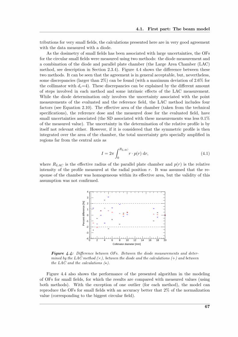
4.1. First part: The beam model
tributions for very small fields, the calculations presented here are in very good agreementwith the data measured with a diode.
As the dosimetry of small fields has been associated with large uncertainties, the OFsfor the circular small fields were measured using two methods: the diode measurement anda combination of the diode and parallel plate chamber (the Large Area Chamber (LAC)method, see description in Section 2.3.4). Figure 4.4 shows the difference between thesetwo methods. It can be seen that the agreement is in general acceptable, but, nevertheless,some discrepancies (larger than 2%) can be found (with a maximum deviation of 2.6% forthe collimator with dc=4). These discrepancies can be explained by the different amountof steps involved in each method and some intrinsic effects of the LAC measurement.While the diode determination only involves the uncertainty associated with the pointmeasurements of the evaluated and the reference field, the LAC method includes fourfactors (see Equation 2.10). The effective area of the chamber (taken from the technicalspecifications), the reference dose and the measured dose for the evaluated field, havesmall uncertainties associated (the SD associated with these measurements was less 0.1%of the measured value). The uncertainty in the determination of the relative profile is byitself not relevant either. However, if it is considered that the symmetric profile is thenintegrated over the area of the chamber, the total uncertainty gets specially amplified inregions far from the central axis as
I = 2π∫ RLAC
0r · p(r) dr, (4.1)
where RLAC is the effective radius of the parallel plate chamber and p(r) is the relativeintensity of the profile measured at the radial position r. It was assumed that the re-sponse of the chamber was homogeneous within its effective area, but the validity of thisassumption was not confirmed.
4
3
2
1
0
-1
-2
-3
-420181614121086420
Per
cent
diff
eren
ce [%
]
Collimator diameter [mm]
Figure 4.4: Difference between OFs. Between the diode measurements and deter-mined by the LAC method (×), between the diode and the calculations (+) and betweenthe LAC and the calculations (?).
Figure 4.4 also shows the performance of the presented algorithm in the modelingof OFs for small fields, for which the results are compared with measured values (usingboth methods). With the exception of one outlier (for each method), the model canreproduce the OFs for small fields with an accuracy better that 2% of the normalizationvalue (corresponding to the biggest circular field).
67

Chapter 4. Discussion
Table 4.1: Measured field sizes and deviations from the CAX for quadratic fieldsin the X and Y directions. The sizes of the fields were determined for 50% of themaximum value. CAX deviations and field sizes were obtained using Mephysto mc2.
Nominal side length Direction Measured size Size difference CAX deviation
[cm] [cm] [cm] [mm]
0.5 X 0.42 -0.08 0.21
0.5 Y 0.72 0.22 0.76
1.0 X 0.73 -0.27 0.18
1.0 Y 1.09 0.09 0.75
5.0 X 4.72 -0.28 0.31
5.0 Y 5.07 0.07 0.76
10.0 X 9.74 -0.26 0.27
10.0 Y 10.06 0.06 0.79
20.0 X 19.79 -0.21 0.13
20.0 Y 20.05 0.05 0.81
30.0 X 29.74 -0.26 0.00
30.0 Y 30.09 0.09 0.89
As seen in Figure 3.7(b), the method also performed well in the modeling of OFs forthe quadratic fields. It was already mentioned that the discrepancies in the small fieldsection of the curve are not due to poor modeling, but rather related to a combination ofeffects: (i) the coarse grid of 1x1 mm2 (in the context of the fields of 5, 10 and 20 mmbeing evaluated), (ii) the uncertainty in the field size (which will be discussed later in thistext) and (iii) the fact that, for these fields, the inner part of the source started to beoccluded by the collimators: due of the steepness of its distribution in this part, a smallvariation in the field size has a great impact on the output variation.
As shown in Section 3.1.3, calculated profiles in water were within the acceptancecriteria of 2%/2mm for the quadratic fields in the Y direction and 2%/0.5mm for thecircular fields. The agreement on the small field penumbras was especially good, as a veryfine calculation grid was used and accurate information on the position and geometry ofthe collimators (aperture and length) for every evaluated field was available. There weretwo sectors with discrepancies of moderate relevance: (i) the central section of the profileusing the collimator with a diameter dc=2 mm (difference ∼2%) and (ii) the tail of thelargest collimator profile (difference ∼2%). The first could be explained by a possiblemisalignment of the diode with the CAX (implying a lower maximum value). A possibleexplanation for the second discrepancy may be related to the interpolation of the PBKor to inaccuracies in the determination of the outer part of the source, more specifically,in the interface section between the inner and the outer part (where the slope is stillpronounced and was obtained from the CF analysis for relatively small fields, thus moreprone to uncertainties). Another explanation could be the spectral variation at off-axis
68
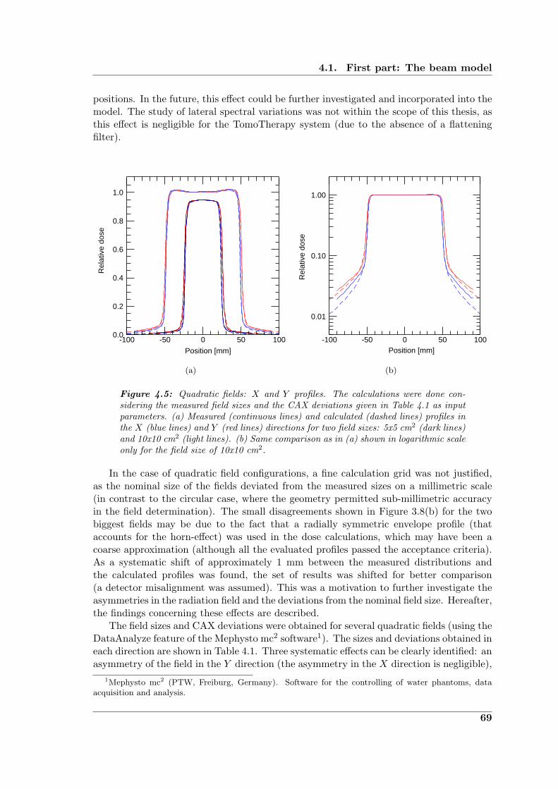
4.1. First part: The beam model
positions. In the future, this effect could be further investigated and incorporated into themodel. The study of lateral spectral variations was not within the scope of this thesis, asthis effect is negligible for the TomoTherapy system (due to the absence of a flatteningfilter).
1.0
0.8
0.6
0.4
0.2
0.0100500-50-100
Rel
ativ
e do
se
Position [mm]
(a)
1.00
0.10
0.01
100500-50-100
Rel
ativ
e do
se
Position [mm]
(b)
Figure 4.5: Quadratic fields: X and Y profiles. The calculations were done con-sidering the measured field sizes and the CAX deviations given in Table 4.1 as inputparameters. (a) Measured (continuous lines) and calculated (dashed lines) profiles inthe X (blue lines) and Y (red lines) directions for two field sizes: 5x5 cm2 (dark lines)and 10x10 cm2 (light lines). (b) Same comparison as in (a) shown in logarithmic scaleonly for the field size of 10x10 cm2.
In the case of quadratic field configurations, a fine calculation grid was not justified,as the nominal size of the fields deviated from the measured sizes on a millimetric scale(in contrast to the circular case, where the geometry permitted sub-millimetric accuracyin the field determination). The small disagreements shown in Figure 3.8(b) for the twobiggest fields may be due to the fact that a radially symmetric envelope profile (thataccounts for the horn-effect) was used in the dose calculations, which may have been acoarse approximation (although all the evaluated profiles passed the acceptance criteria).As a systematic shift of approximately 1 mm between the measured distributions andthe calculated profiles was found, the set of results was shifted for better comparison(a detector misalignment was assumed). This was a motivation to further investigate theasymmetries in the radiation field and the deviations from the nominal field size. Hereafter,the findings concerning these effects are described.
The field sizes and CAX deviations were obtained for several quadratic fields (using theDataAnalyze feature of the Mephysto mc2 software1). The sizes and deviations obtained ineach direction are shown in Table 4.1. Three systematic effects can be clearly identified: anasymmetry of the field in the Y direction (the asymmetry in the X direction is negligible),
1Mephysto mc2 (PTW, Freiburg, Germany). Software for the controlling of water phantoms, dataacquisition and analysis.
69
Chapter 4. Discussion
a negative deviation from the nominal field size in the X direction and a positive deviationfrom the nominal field size in the Y direction. The field size variation in the X directionis quite significant; of the order of -2 to -3 mm. The rest of the variations are within 1 mmand can be explained by detector positioning effects. However, it is interesting to notethe concordance of the CAX and size deviations in the Y direction with the predictionsmade in Section 4.1.1, which were based on the analysis of a strip-integral measured fora 6x6 cm2 field in the Y direction (see Figure 4.1(b)). The slit-method predicted a 1 mmincrease from the nominal field size in the Y direction, shifted 0.8 mm from the CAX,which is in very good agreement with the measured field size deviation (0.97±0.06 mm,x± σ) and CAX deviation (0.79±0.05 mm, x± σ).
Figure 4.5(a) shows the comparison between measured and calculated profiles in the Xand Y directions for two different quadratic fields (5x5 and 10x10 cm2 in size) consideringsize and symmetry effects, which can be clearly identified. In general, a very good agree-ment between measured and calculated distributions can be seen. Now, looking at theprofiles in a logarithmic scale (Figure 4.5(b)), it can be seen that the umbra region of theprofiles (low dose region, outside the radiation field) is not perfectly modeled. This canbe explained on the basis that transmission and leakage effects have not been consideredin the calculation algorithm, as perfect collimators were assumed. It can be seen that thedeveloped model reproduces the umbra better in the Y direction. This is not a surprise,as the Y -jaws are thicker than the MLC (which shapes the field in the X direction) andthere is no contribution from interleaf leakage.
4.1.5 On the advantages and limitations of the model
After a thorough evaluation of most of the aspects concerning the implementation andvalidation process for the presented model, a critical view on the strengths and weaknessesof this algorithm can be presented.
Advantages
The algorithm was successfully validated, predicting accurately OFs and planar dose dis-tributions in water from very small to large field sizes, making it a useful QA tool for theperformance of the linac. As the complete range of evaluated field sizes was well repro-duced, the transformation of relative values into absolute dose becomes straightforward(only a dose conversion factor measured in a reference field is needed), which enables thismethod to be used as an alternative to the conventional dosimetry of small fields. As aby-product of the slit-method (used for the reconstruction of the source), accurate infor-mation on the disposition of the components in the linac head (collimators) that can beused to predict the exact geometry of the radiation field was obtained. This by itself canbe used as a supplemental QA test.
Recently, Djouguela et al. (2009) have investigated an analytical approach to reproducedose profiles of narrow photon beams. They have used an analytic/parametric convolutionkernel based on the Lorentz function that can account for both, the source extensionand the energy transport of secondary electrons in a single radially symmetric function.They found a very good agreement between a set of measured and calculated profilesin the range of 10 to 30 mm in side length (at three different depths for two differentenergies). Even though they present an attractive, purely mathematical approach, themodel described throughout this thesis provides a more general and physically meaningful
70
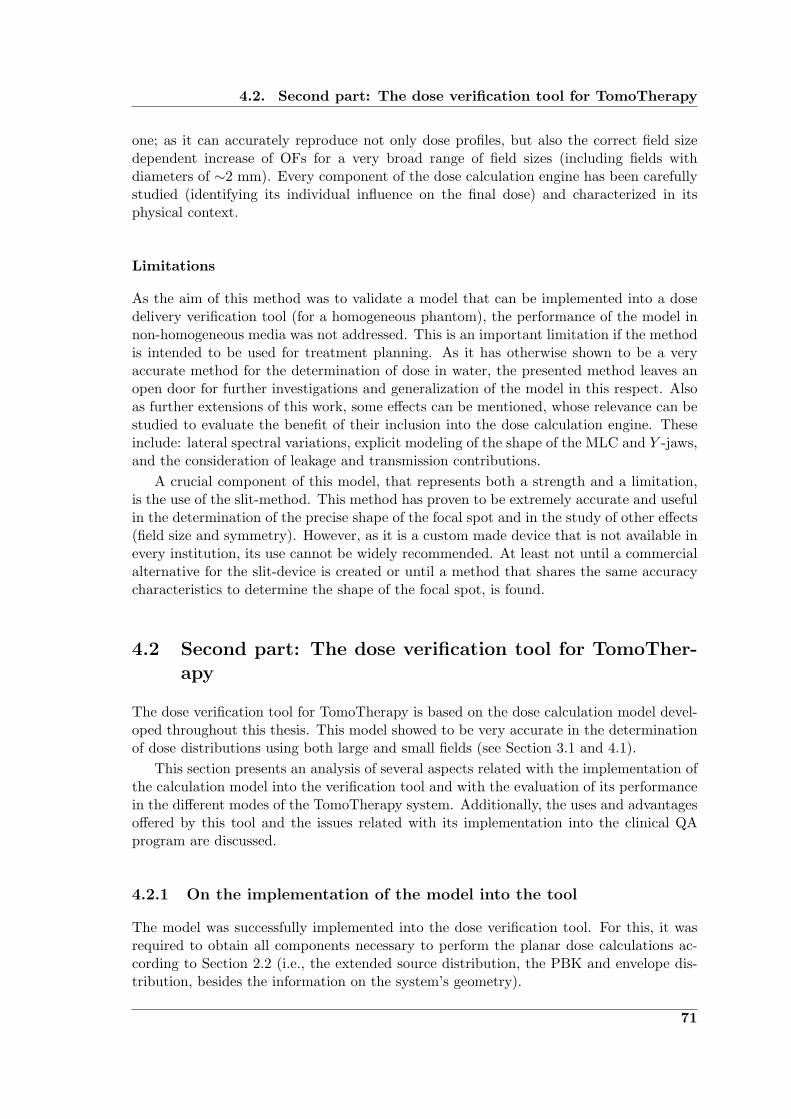
4.2. Second part: The dose verification tool for TomoTherapy
one; as it can accurately reproduce not only dose profiles, but also the correct field sizedependent increase of OFs for a very broad range of field sizes (including fields withdiameters of ∼2 mm). Every component of the dose calculation engine has been carefullystudied (identifying its individual influence on the final dose) and characterized in itsphysical context.
Limitations
As the aim of this method was to validate a model that can be implemented into a dosedelivery verification tool (for a homogeneous phantom), the performance of the model innon-homogeneous media was not addressed. This is an important limitation if the methodis intended to be used for treatment planning. As it has otherwise shown to be a veryaccurate method for the determination of dose in water, the presented method leaves anopen door for further investigations and generalization of the model in this respect. Alsoas further extensions of this work, some effects can be mentioned, whose relevance can bestudied to evaluate the benefit of their inclusion into the dose calculation engine. Theseinclude: lateral spectral variations, explicit modeling of the shape of the MLC and Y -jaws,and the consideration of leakage and transmission contributions.
A crucial component of this model, that represents both a strength and a limitation,is the use of the slit-method. This method has proven to be extremely accurate and usefulin the determination of the precise shape of the focal spot and in the study of other effects(field size and symmetry). However, as it is a custom made device that is not available inevery institution, its use cannot be widely recommended. At least not until a commercialalternative for the slit-device is created or until a method that shares the same accuracycharacteristics to determine the shape of the focal spot, is found.
4.2 Second part: The dose verification tool for TomoTher-apy
The dose verification tool for TomoTherapy is based on the dose calculation model devel-oped throughout this thesis. This model showed to be very accurate in the determinationof dose distributions using both large and small fields (see Section 3.1 and 4.1).
This section presents an analysis of several aspects related with the implementation ofthe calculation model into the verification tool and with the evaluation of its performancein the different modes of the TomoTherapy system. Additionally, the uses and advantagesoffered by this tool and the issues related with its implementation into the clinical QAprogram are discussed.
4.2.1 On the implementation of the model into the tool
The model was successfully implemented into the dose verification tool. For this, it wasrequired to obtain all components necessary to perform the planar dose calculations ac-cording to Section 2.2 (i.e., the extended source distribution, the PBK and envelope dis-tribution, besides the information on the system’s geometry).
71

Chapter 4. Discussion
Extended source and head scatter effects
In Figure 4.6(a), the reconstructed distribution of the TomoTherapy source (blue line),obtained using the slit-method, is compared with the distribution found for the linac’sbeam (red line). It can be seen that the TomoTherapy focal spot has a larger FWHM (of0.72±0.05 mm) than the one obtained for the linac and that the intensity (for the sameradial positions) remains higher at radial positions .5 mm (that approximately coincideswith the position from which a background signal can be identified on the red line).From this position on, the intensity of the TomoTherapy source continues to decreaseuntil a background signal can be identified (of almost one order of magnitude lower thanfor the linac case). This difference in the background intensity is related to the factthat the absence of flattening filter in the TomoTherapy system reduces significantly thehead scatter contributions and thus, the detector signal used for the reconstruction (strip-integral) is less “contaminated” by scatter radiation.
The influence of the background signal in the determination of the correct extendedsource (able to reproduce the field size dependence of the CFs) can be better understoodfrom Figure 4.6(b), where CFs were calculated (according to Equation 2.5) using thedifferent reconstructed distributions and assuming the same geometric configuration (thedetector is positioned at 100 cm from the source and the circular fields are producedby perfect collimators located at 20 cm from the source). It can be seen that the CFdistribution using the TomoTherapy reconstructed source (blue line) already resemblesthe expected field size dependence (Figure 3.14), whereas using the linac’s distribution(red) the distribution shows a clear overestimation of the expected increase of CF withincreasing in field size (Figure 3.7).
100
10-2
10-4
10-6
20151050Radial distance [mm]
Rel
ativ
e in
tens
ity
(a)
1.2
1.0
0.8
0.6
0.4
0.2
0.0140120100806040200
CF
Field diameter [mm]
(b)
Figure 4.6: Comparison of reconstructed focal spots and the associated CF distribu-tions. (a) Reconstructed radial distributions of the linac (red line) and the TomoTher-apy (blue line) sources. (b) Comparison between the variation in CF associated withthe increase in field size using the linac’s (red line) and TomoTherapy’s (blue line)reconstructed source distributions.
72
4.2. Second part: The dose verification tool for TomoTherapy
Pencil beam kernel and percentage depth dose curves
The PBK obtained by the method described in Section 2.3.2, proved to be appropriateto model the depth dependence of the dose in the central axis for different field sizes (asshown in Figure 3.11) and, in combination with the extended source, was also able toreproduce both the increase of the OFs depending on the field size (Figure 3.14) and theshape of the penumbra for different field configurations (see Figure 3.15 and 3.16).
100
80
60
40
20
250200150100500
PD
D [%
]
Depth [mm]
Figure 4.7: Comparison of calculated PDDs for the linac (red line) and for theTomoTherapy system (blue line) considering a nominal field size of 5x5 cm2 andSSDs of 100 and 85 cm respectively.
Although the 6 MV beam of the conventional linac used in the validation of the dosecalculation model and the TomoTherapy beam have the same nominal energy, they havedifferent spectral characteristics (see Section 2.4.2). The energy characteristics of the beamare reflected in its PDD curve. Figure 4.7 shows the comparison between the calculatedPDD distributions for the linac and for the TomoTherapy beam, using the same nominalfield size (of 5x5 cm2). One of the main reasons of the spectral differences is the flatteningfilter, which filters the photons from the low energy end of the spectrum and thus, makesthe linac spectrum harder than the one of the TomoTherapy beam. This, increases the(mean) forward range of the secondary electrons, thus, the depth of maximum dose (wherethe condition of CPE is achieved) is shifted to a deeper position with respect to theTomoTherapy case.
4.2.2 On the evaluation of the tool
After comparing measured and calculated OFs and dose profiles for different field config-urations in the static and dynamic delivery modes, it was found that they were in verygood agreement (within the acceptance criteria of 2%/2mm globally defined).
Most of the small discrepancies between measured and calculated profiles and OFs inthe static mode (see Figure 3.13 and 3.14) can be associated with interpolation, convolutionor voxel averaging effects (the calculation grid was of 1x1x1 mm3). Nevertheless, theinfluence of other effects related to the MLC hardware (i.e., the exact shape and positionof the leaves) could not be discarded as the approximation of perfect collimators was used.
73

Chapter 4. Discussion
Figure 3.15 shows that the penumbras in the X and Y directions are well modeled bythe combination of extended source and PBK effects. Furthermore, the inclusion of theleakage contribution in the X direction was shown to be sufficient to accurately modelthe “umbra” of the distributions down to ∼1% of the maximum dose, in contrast toresults obtained for the linac (see Figure 4.5(b)), were the leakage contributions were notconsidered. The fact that the agreement in the Y direction is very good, is based on the factthat the jaws that define the field size in the longitudinal direction were made of tungstenof up to 23 cm in thickness and, therefore, the contributions due to the transmission ofphotons through the collimators in this direction was negligible. As seen in Figure 3.16,the tool was also found to be well suited to model dose distribution in asymmetric andcomplex field configurations.
From the dynamic tests, it was found that the verification tool was able to reproducemeasured profiles within 2%/2mm for simple beam configurations. By looking at themeasured profiles for this simple configurations, the effect of temporal variations in one ormore of the beam parameters was identified (because the “plateau” regions were not flatas expected for constant parameters). Once the sinograms (and treatment parameters) ofpatients become available, the application of this tool as a patient specific QA test shouldbe evaluated.
4.2.3 On the parameter variations
The dose verification tool is not only useful as a dose verification system, but also can beuse to study more deeply this dynamic delivery technique and identify the individual roleof the different beam parameters in the final outcome of the treatment.
As the overall performance of the system depends on the performance and synchronyof the MLC, gantry, couch and linac. Random and systematic variations were introducedto the parameters that are considered constant in the planning of the treatments (beamoutput, couch velocity and gantry speed). The results of this study were presented inSection 3.2.3.
It was found that none of the variations introduced (see Figure 3.19) yielded deviationsgreater than 3%/3mm from a reference helical distribution (for which the parameters wereassumed to be constant during the complete treatment). It was interesting to see thatrandom variations of the beam output (of ±2%) had almost no influence in the integraldose (with a maximum observed deviation of 0.7% from the reference value). Flynn et al.(2008) investigated the effect of output variations (random and systematic) in the integraldose for different clinical cases. They found that systematic and random variations tendto cancel out throughout the treatment and, therefore, the ±2% threshold of the beamoutput (recommended by Fenwick et al. 2004) was shown to be too conservative. Thisconclusions are in agreement with the presented results.
4.2.4 On the implementation of the tool into the quality assurance pro-gram
As previously described, it was found that the developed tool offers a very useful approachto study the TomoTherapy delivery system and to test its performance using the differentavailable modes (static, topographic, rotational and helical). Therefore, it can be used asa supplemental dosimetric QA procedure for the system. It was possible to visualize thecalculated distributions not only in one and two-dimensional representations (as shown in
74

4.2. Second part: The dose verification tool for TomoTherapy
Figure 3.17), but also in three-dimensional intensity maps and isosurfaces (as shown inFigure 4.8). The availability of this feature is indeed desirable in certain cases (e.g., theuse of isosurfaces to study and identify variations in the “thread” effect by using differentpitch values).
(a) (b)
Figure 4.8: 3-D visualization of an helical dose distribution delivered on the virtualcylindrical phantom. (a) Main planes and contours. (b) Isosurface and 3-D distribu-tion.
The dose verification tool would certainly benefit from the implementation of compari-son tools (e.g., the 2-D gamma index distribution) into a stand alone application, in whichall the input parameters (and output representations) can be interactively controlled bythe user. In this way, its introduction into the routine QA program of the system would beeasier. It was not within the scope of this thesis to address this practical implementationissues. However, considering the usability range of this tool, they should certainly be ad-dressed as a continuation of this work. Also, a recommendation for the further expansionof the presented study, is to increase the flexibility of the phantom shape, positioning andcomposition (once the dose engine is validated for non-homogeneous media).
75

“The universe is full of magical things patiently wait-ing for our wits to grow sharper.”
Eden Phillpotts (1862-1960)
5Concluding Remarks
In this final chapter, the work presented throughout this thesis is summarized. An outlooktogether with suggestions for future research that can extend its scope and address itscurrent limitations is also given.
5.1 Summary
This dissertation presents the implementation of a dose calculation tool for the verificationof dose delivered to a homogenous phantom using the TomoTherapy system. This tool isbased on a dose calculation model developed to accurately reproduce dose distributions forsmall fields. This procedure can be implemented as a supplemental check for the alreadyestablished dosimetric QA program of the TomoTherapy system.
In Chapter 2, the main physical aspects of the energy deposition in matter for clini-cal photons beams and the development of the dose calculation methods, according to thetechnological evolution and the demanding uncertainty requirements, have been presented.The advantages and challenges posed by state-of-the-art techniques used in photon radio-therapy have been pointed out. According to this, a model that serves to account for thenon-conventional conditions imposed by the use of these techniques has been developed.A special focus has been given to TomoTherapy. Within this context, the system hasbeen described and the present QA crisis due to the accelerated technological advanceshas been unveiled. These advances have yielded the commercialization of non-standardsystems, making it impossible (in certain cases, e.g., TomoTherapy) to apply the conven-tional dosimetry protocols, and thus, complicating the establishment of new standardizedrecommendations. A QA program of the TomoTherapy system has been presented and astrategy to study this delivery technique and to verify the dose delivered to a homogeneousphantom was proposed.
The developed model was validated for a 6 MV beam produced by a conventionallinac. In the first part of Chapter 3, the results of the main model parameters and ofthe validation tests were shown. The shape of the extended source, reconstructed using acombination of a slit-method and CF analysis, was found to have a FWHM of 0.50±0.08
77

Chapter 5. Concluding Remarks
mm. The model was successfully validated, as it was able to accurately reproduce planardose profiles and OFs in water with an agreement better than 2%/2mm for quadraticfields (calculation grid of 1x1 mm2) and better than 2%/0.5mm for fields performed bystereotactic collimators (calculation grid of 0.1x0.1 mm2). The second part of Chapter 3included the results of the tests performed to the dose verification tool for TomoTherapy.For simple MLC configurations in static and dynamic modes, the results were found tobe in agreement with the validation of the model (i.e., better than 2%/2mm using acalculation grid of 1x1 mm2). The studied parameter variations revealed that: (i) mostof the random variations cancel out throughout the treatment and (ii) the systematicsproduce variations in the overall treatment that remain below 3%/3mm.
Chapter 4 included the analysis of the results presented in the previous chapter. Itwas found that the reconstructed source size is in agreement with the FWHM foundby Jaffray et al. (1993). The inclusion of the extended source (including head scattercontributions) into the pencil beam kernel calculations proved to be adequate, as themodel was able to provide accurate modeling of the penumbra and output of the beamfor a broad range of field sizes. Thus, making the transformation into absolute dosestraightforward and providing an alternate method to the conventional dosimetry of smallfields. Concerning the TomoTherapy results in static mode, it was confirmed that thelow head scatter contributions due to the absence of a flattening filter result in an almostnegligible intensity of the outer part of the source. The reconstructed source proved tobe efficient in reproducing the measured penumbras. In the dynamic mode, althoughonly simple cases were studied, the tool was found to be particularly useful to study theinfluence of variations in beam output, gantry speed and table position on the uncertaintyof the integral dose. The application of this approach as a supplemental QA procedurewas assessed and the limitations of it were discussed.
One of the main conclusions of this work is that having an independent dose calculationmethod is a useful and feasible supplemental QA procedure for the TomoTherapy deliverysystem. The model presented in this work provides a calculation tool with the capabilityof handling the narrow beam conditions that are present in TomoTherapy delivered treat-ments. Nevertheless, the approach developed in this thesis still has some limitations thatneed to be addressed in future studies. In the next section, suggestions to be consideredas an extension of this project are presented.
5.2 Perspectives
As discussed in Chapter 4, the concepts and methods used in the implementation of thetool are based on simple theoretical considerations, and therefore, straightforward to beperformed (once the input data has been obtained). Although the developed tool provedto be sufficiently accurate and useful for the verification of dose distributions delivered(in a homogeneous medium) by the TomoTherapy system, it would certainly benefit fromfurther developments.
After finishing this project, it was realized that the accuracy of the calculation toolcould be further improved by including more effects that were not explicitly modeled inthis approach. These effects include a complete characterization of the MLC (taking intoaccount that they are not perfectly aligned with the source) and the inclusion of the couchinto the calculation algorithm.
It would be desirable that the dose verification tool was implemented into a stand-alone
78

5.2. Perspectives
application with a user-friendly interface in order to ease its incorporation into the clinicalQA program of the system. Considering the usefulness and potential of the presentedmethod, it would be worth to continue this work by implementing such an application. Inthis way, after inputting the basic parameters (i.e., source shape, PBK distribution andenvelope profile) the user could easily control the treatment parameters and the desiredoutput form (point, profile or plane calculation) in an interactive way. The possibility toinput reference data and the availability of comparison tools, such as the gamma indexcalculation, would also be desirable to ease the integration of this procedure into theworkflow of the QA program.
To extend the application of this tool from its current state of supplemental deliveryverification procedure into a TPS verification system, it is necessary that the model handlesinhomogeneities and performs calculations using the CT data-set of the patient. For thispurpose, the pencil beam approach may not be adequate anymore, as it can only accountfor inhomogeneities in the forward direction by kernel scaling (it can not correct for lateralinhomogeneities). Therefore, it might be appropriate to use a collapsed-cone convolutionapproach, increasing the complexity of the algorithm.
79

Bibliography
Ahnesjo A 1989 Collapsed cone convolution of radiant energy for photon dose calculationin heterogeneous media Med. Phys. 16(4), 577–592.
Ahnesjo A 1994 Analytic modeling of photon scatter from flattening filters in photontherapy beams Med. Phys. 21(8), 1227–1235.
Ahnesjo A, Andreo P and Brahme A 1987 Calculation and application of point spread func-tions for treatment planning with high energy photon beams Acta Oncologica 26(1), 49–56.
Ahnesjo A and Aspradakis M M 1999 Dose calculations for external photon beams inradiotherapy Phys. Med. Biol. 44(11), R99–R155.
Ahnesjo A, Saxner M and Trepp A 1992 A pencil beam model for photon dose calculationMed. Phys. 19(2), 263–273.
Ahnesjo A and Trepp A 1991 Acquisition of the effective lateral energy fluence distributionfor photon beam dose calculations by convolution models Phys. Med. Biol. 36(7), 973–985.
Alfonso R, Andreo P, Capote R, Huq M S, Kilby W, Kjall P, Mackie T R, Palmans H,Rosser K, Seuntjens J, Ullrich W and Vatnitsky S 2008 A new formalism for referencedosimetry of small and nonstandard fields Med. Phys. 35(11), 5179–5186.
Almond P R, Biggs P J, Coursey B M, Hanson W F, Huq M S, Nath R and RogersD W O 1999 AAPM’s TG-51 protocol for clinical reference dosimetry of high-energyphoton and electron beams Med. Phys. 26(9), 1847–1870.
Andreo P, Burns D T, Hohlfeld K, Huq M S, Kanai T, Laitano F, Smyth V and VynckierS 2000 Absorbed dose determination in external beam radiotherapy: An internationalcode of practice for dosimetry based on standards of absorbed dose to water iaea tech-nical report series no 398 Technical report IAEA Vienna, Austria.
Andreo P and Ortiz-Lopez P 1997 Tecdoc-1040: Quality assurance in radiotherapy Tech-nical report IAEA Vienna, Austria.
Balog J, Holmes T and Vaden R 2006 Helical tomotherapy dynamic quality assuranceMed. Phys. 33(10), 3939–3950.
Balog J, Olivera G and Kapatoes J 2003 Clinical helical tomotherapy commissioningdosimetry Med. Phys. 30(12), 3097–3106.
Balog J and Soisson E 2008 Helical tomotherapy quality assurance Int. J. Radiation On-cology Biol. Phys. 71(1, Supplement 1), S113–S117.
81

Bibliography
Belletti S, Dutreix A, Garavaglia G, Gfirtner H, Haywood J, Jessen K A, Lamm I L, Mi-jnheer B, Noel A, Nusslin F, Rosenow U, Schneider P, Seelentag W, Sheriff S, SvenssonH and Thwaites D 1996 Quality assurance in radiotherapy: The importance of MedicalPhysics staffing levels. Recommendations from an ESTRO/EFOMP joint task groupRad. Oncol. 41(1), 89–94.
Berger M J and Seltzer S M 1982 Stopping powers and ranges of electrons and positronsTechnical report National Bureau of Standards Report NBSIR 822550 Washington, DC,United Sates of America.
BIPM, IEC, IFCC, ISO, IUPAC, IUPAP and OIML 1995 Guide to the Expression ofUncertainty in Measurement International Organisation for Standardisation. Geneva,Switzerland.
Bortfeld T 2006 IMRT: A review and preview Phys. Med. Biol. 51(13), R363–R379.
Bortfeld T, Schlegel W and Rhein B 1993 Decomposition of pencil beam kernels for fastdose calculations in three-dimensional treatment planning Med. Phys. 20(2), 311–318.
Bourland J D and Chaney E L 1992 A finite-size pencil beam model for photon dosecalculations in three dimensions Med. Phys. 19(6), 1401–1412.
Boyer A, Biggs P, Galvin J, Klein E, LoSasso T, Low D, Mah K and Yu C 2001 BasicApplications of Multileaf Collimators: Report of AAPM radiation therapy task groupno. 50 Technical report AAPM Madison, WI, United Sates of America.
Boyer A, Biggs P, Galvin J, Klein E, LoSasso T, Low D, Mah K and Yu C 2004 Tissueinhomogeneity corrections for megavoltage photon beams: Report of AAPM radiationtherapy task group no. 65 Technical report AAPM Madison, WI, United Sates of Amer-ica.
Boyer A and Mok E 1985 A photon dose distribution model employing convolution calcu-lations Med. Phys. 12(2), 169–177.
Boyle P and Levin B, eds 2008 World Cancer Report 2008 International Agency for Re-search on Cancer (IARC).
Brahme A, Roos J E and Lax I 1982 Solution of an integral equation encountered inrotation therapy Phys. Med. Biol. 27(10), 1221–1229.
Broggi S, Cattaneo G M, Molinelli S, Maggiulli E, Vecchio A D, Longobardi B, PernaL, Fazio F and Calandrino R 2008 Results of a two-year quality control program for ahelical tomotherapy unit Rad. Oncol. 86(2), 231–241.
Calcina C S G, de Oliveira L N, de Almeida C E and de Almeida A 2007 Dosimetricparameters for small field sizes using fricke xylenol gel, thermoluminescent and filmdosimeters, and an ionization chamber Phys. Med. Biol. 52(5), 1431–1439.
Caprile P and Hartmann G H 2009 Development and validation of a beam model applicableto small fields Phys. Med. Biol. 54(10), 3257–3268.
Ceberg C P, Bjarngard B E and Zhu T C 1996 Experimental determination of the dosekernel in high-energy x-ray beams Med. Phys. 23(4), 505–511.
82
Bibliography
Childress N L, White R A, Bloch C, Salehpour M, Dong L and Rosen I I 2005 Retrospectiveanalysis of 2d patient-specific imrt verifications Med. Phys. 32(4), 838–850.
Chui C, LoSasso T and Palm A 2003 Computational algorithms for independent veri-fication of IMRT. In: A Practical Guide to Intensity-Modulated Radiation Therapy(Madison, WI: Med. Phys. Publishing) pp. 83–101.
Chui C S and Mohan R 1988 Extraction of pencil beam kernels by the deconvolutionmethod Med. Phys. 15(2), 138–144.
Crop F, Reynaert N, Pittomvils G, Paelinck L, Gersem W D, Wagter C D, Vakaet L, NeveW D and Thierens H 2007 Monte Carlo modeling of the moduleaf miniature mlc forsmall field dosimetry and quality assurance of the clinical treatment planning systemPhys. Med. Biol. 52(11), 3275–3290.
Cunningham J R 1972 Scatter-air ratios Phys. Med. Biol. 17(1), 42–51.
Das I J, Ding G X and Ahnesjo A 2008 Small fields: Nonequilibrium radiation dosimetryMed. Phys. 35(1), 206–215.
Day M J 1950 A note on the calculation of dose in x-ray fields Br. J. Radiol. 23, 368–369.
Delaney G, Jacob S, Featherstone C and Barton M 2003 Radiotherapy in cancer care:Estimating optimal utilization from a review of evidence-based clinical guidelines Tech-nical report Collaboration for Cancer Outcomes Research and Evaluation (CCORE)Liverpool Hospital, Sydney, Australia.
Djouguela A, Harder D, Kollhoff R, Foschepoth S, Kunth W, Ruhmann A, Willborn Kand Poppe B 2009 Fourier deconvolution reveals the role of the lorentz function as theconvolution kernel of narrow photon beams Phys. Med. Biol. 54(9), 2807–2827.
Dutreix A 1984 When and how can we improve precision in radiotherapy? Radiother. andOncol. 2(4), 275–292.
Eklof A, Ahnesjo A and Brahme A 1990 Photon beam energy deposition kernels for inverseradiotherapy planning Acta Oncol. 29(4), 447–454.
El-Khatib E and Battista J J 1984 Improved lung dose calculation using tissue–maximumratios in the batho correction Med. Phys. 11(3), 279–286.
Ezzell G A, Galvin J M, Low D, Palta J R, Rosen I, Sharpe M B, Xia P, Xiao Y, XingL and Yu C X 2003 Guidance document on delivery, treatment planning, and clinicalimplementation of IMRT: Report of the IMRT subcommittee of the AAPM radiationtherapy committee Med. Phys. 30(8), 2089–2115.
Fenwick J D, Tome W A, Jaradat H A, Hui S K, James J A, Balog J P, DeSouza C N,Lucas D B, Olivera G H, Mackie T R and Paliwal B R 2004 Quality assurance of ahelical tomotherapy machine Phys. Med. Biol. 49(13), 2933–2953.
Flynn R T, Kissick M W, Mehta M P, Olivera G H, Jeraj R and Mackie T R 2008 Theimpact of linac output variations on dose distributions in helical tomotherapy Phys.Med. Biol. 53(2), 417–430.
83

Bibliography
Fraass B, Doppke K, Hunt M, Kutcher G, Starkschall G, Stern R and Dyke J V 1998 Amer-ican association of physicists in medicine radiation therapy committee Task Group 53:Quality assurance for clinical radiotherapy treatment planning Med. Phys. 25(10), 1773–1829.
Gaskill J D 1978 Linear systems, Fourier transforms, and optics Wiley Series in Pure andApplied Optics, New York: Wiley, 1978.
Gibbons J, Smith K, Cheek D and Rosen I 2009 Independent calculation of dose from ahelical tomotherapy unit J. Appl. Clin. Med. Phys. 10(1), 103–119.
Giraud P, Elles S, Helfre S, Rycke Y D, Servois V, Carette M F, Alzieu C, Bondiau P Y,Dubray B, Touboul E, Housset M, Rosenwald J C and Cosset J M 2002 Conformalradiotherapy for lung cancer: Different delineation of the gross tumor volume (GTV)by radiologists and radiation oncologists Radiother. Oncol. 62(1), 27–36.
Hobbie R and Roth B 2007 Intermediate physics for medicine and biology Springer.
ICRU 1976 Determination of absorbed dose in a patient irradiated by beams of x orgamma rays in radiotherapy procedures Technical report International Commission onRadiation Units and Measurements (ICRU) Washington, DC, United Sates of America.
Jaffray D A, Battista J J, Fenster A and Munro P 1993 X-ray sources of medical linearaccelerators: Focal and extra-focal radiation Med. Phys. 20(5), 1417–1427.
Jelen U 2007 Development and verification of a high-precision dose calculation algorithmfor IMRT treatment planning PhD thesis AGH University of Science and Technology,Poland.
Jeraj R, Mackie T R, Balog J, Olivera G, Pearson D, Kapatoes J, Ruchala K and Reckw-erdt P 2004 Radiation characteristics of helical tomotherapy Med. Phys. 31(2), 396–404.
Khan F M, Sewchand W, Lee J and Williamson J F 1980 Revision of tissue-maximumratio and scatter-maximum ratio concepts for cobalt 60 and higher energy x-ray beamsMed. Phys. 7(3), 230–237.
Kissick M W, Fenwick J, James J A, Jeraj R, Kapatoes J M, Keller H, Mackie T R,Olivera G and Soisson E T 2005 The helical tomotherapy thread effect Med. Phys.32(5), 1414–1423.
Kopka H and Daly P W 1977 Donner Algorithms for Reconstructive Tomography UsersManual Lawrence Berkeley Laboratory, Publication No. 214.
Kutcher G J, Coia L, Gillin M, Hanson W F, Leibel S, Morton R J, Palta J R, Purdy J A,Reinstein L E, Svensson G K, Weller M and Wingfield L 1994 Comprehensive QA forradiation oncology: Report of AAPM radiation therapy committee task group 40 Med.Phys. 21(4), 581–618.
Leunens G, Menten J, Weltens C, Verstraete J and van der Schueren E 1993 Quality as-sessment of medical decision making in radiation oncology: Variability in target volumedelineation for brain tumours Radiother. Oncol. 29(2), 169–175.
84

Bibliography
Low D A, Chao K, Mutic S, Gerber R L, Perez C A and Purdy J A 1998 Quality assuranceof serial tomotherapy for head and neck patient treatments Int. J. Radiation OncologyBiol. Phys. 42(3), 681–692.
Low D A and Dempsey J F 2003 Evaluation of the gamma dose distribution comparisonmethod Med. Phys. 30(9), 2455–2464.
Low D A, Harms W B, Mutic S and Purdy J A 1998 A technique for the quantitativeevaluation of dose distributions Med. Phys. 25(5), 656–661.
Mackie T R 2006 History of tomotherapy Phys. Med. Biol. 51(13), R427–R453.
Mackie T R, Bielajew A F, Rogers D W O and Battista J J 1988 Generation of photonenergy deposition kernels using the EGS Monte Carlo code Phys. Med. Biol. 33(1), 1–20.
Mackie T R, Holmes T, Swerdloff S, Reckwerdt P, Deasy J O, Yang J, Paliwal B andKinsella T 1993 Tomotherapy: A new concept for the delivery of dynamic conformalradiotherapy Med. Phys. 20(6), 1709–1719.
Mackie T R, Scrimger J W and Battista J J 1985 A convolution method of calculatingdose for 15-mv x rays Med. Phys. 12(2), 188–196.
Mainegra-Hing E, Rogers D W O and Kawrakow I 2005 Calculation of photon energydeposition kernels and electron dose point kernels in water Med. Phys. 32(3), 685–699.
Mijnheer B J, Battermann J J and Wambersie A 1987 What degree of accuracy is requiredand can be achieved in photon and neutron therapy? Radiother. Oncol. 8(3), 237–52.
Mohan R, Chui C and Lidofsky L 1985 Energy and angular distributions of photons frommedical linear accelerators Med. Phys. 12(5), 592–597.
Mohan R, Chui C and Lidofsky L 1986 Differential pencil beam dose computation modelfor photons Med. Phys. 13(1), 64–73.
Mohan R and Chui C S 1987 Use of fast fourier transforms in calculating dose distribu-tions for irregularly shaped fields for three-dimensional treatment planning Med. Phys.14(1), 70–77.
Munro P, Rawlinson J A and Fenster A 1988 Therapy imaging: Source sizes of radiother-apy beams Med. Phys. 15(4), 517–524.
Nath R, Biggs P J, Bova F J, Ling C C, Purdy J A, van de Geijn J and Weinhous M S1994 AAPM code of practice for radiotherapy accelerators: Report of AAPM radiationtherapy task group no. 45 Med. Phys. 21(7), 1093–1121.
Nilsson B and Brahme A 1981 Contamination of high-energy photon beams by scatteredphotons. Strahlentherapie 157(3), 181–6.
Nyholm T, Olofsson J, Ahnesjo A, Georg D and Karlsson M 2006 Pencil kernel correctionand residual error estimation for quality-index-based dose calculations Phys. Med. Biol.51(23), 6245–6262.
Olofsson J 2006 Developing and Evaluating Dose Calculation Models for Verification ofAdvanced Radiotherapy PhD thesis Umea University, Sweden.
85

Bibliography
Palta J R, Liu C and Li J G 2008a Current external beam radiation therapy qualityassurance guidance: Does it meet the challenges of emerging image-guided technologies?Int. J. Radiation Oncology Biol. Phys. 71(1, Supplement 1), S13–S17.
Palta J R, Liu C and Li J G 2008b Quality assurance of intensity-modulated radiationtherapy Int. J. Radiation Oncology Biol. Phys. 71(1, Supplement 1), S108–S112.
Pappas E, Maris T G, Zacharopoulou F, Papadakis A, Manolopoulos S, Green S andWojnecki C 2008 Small SRS photon field profile dosimetry performed using a pinpointair ion chamber, a diamond detector, a novel silicon-diode array (DOSI), and polymergel dosimetry. analysis and intercomparison Med. Phys. 35(10), 4640–4648.
Rathee S, McClean B A and Field C 1993 An improved method for rebinning kernels fromcylindrical to cartesian coordinates Med. Phys. 20(5), 1343–1351.
Rogers D, Kawrakow I, Seuntjens J, Walters B and Mainegra-Hing E 2001 NRC usercodes for EGSnrc Technical report National Research Council of Canada Report NoPIRS-702.
Sanchez-Doblado F, Hartmann G H, Pena J, Rosello J V, Russiello G and Gonzalez-Castano D M 2007 A new method for output factor determination in mlc shaped narrowbeams Physica Medica 23(2), 58–66.
Sarkar V, Lin L, Shi C and Papanikolaou N 2007 Quality assurance of the multileaf collima-tor with helical tomotherapy: Design and implementation Med. Phys. 34(7), 2949–2956.
Schlegel W and Mahr A, eds 2007 3D Conformal Radiation Therapy - A MultimediaIntroduction to Methods and Techniques, 2nd revised and enhanced edition. MultimediaDVD. Springer.
Schneider W, Bortfeld T and Schlegel W 2000 Correlation between CT numbers and tissueparameters needed for Monte Carlo simulations of clinical dose distributions Phys. Med.Biol. 45(2), 459–478.
Scholz C, Schulze C, Oelfke U and Bortfeld T 2003 Development and clinical applicationof a fast superposition algorithm in radiation therapy Radiother. Oncol. 69(1), 79–90.
Scott A J D, Nahum A E and Fenwick J D 2008 Using a Monte Carlo model to predictdosimetric properties of small radiotherapy photon fields Med. Phys. 35(10), 4671–4684.
Sharpe M B and Battista J J 1993 Dose calculations using convolution and superpositionprinciples: The orientation of dose spread kernels in divergent x-ray beams Med. Phys.20(6), 1685–1694.
Sontag M, Battista J, Bronskill M and Cunningham J 1977 Implications of computedtomography for inhomogeneity corrections in photon beam dose calculations Radiology124(1), 143–149.
Sontag M and Cunningham J 1978 The equivalent tissue-air ratio method for makingabsorbed dose calculations in a heterogeneous medium Radiology 129(3), 787–794.
Sontag M R and Cunningham J R 1977 Corrections to absorbed dose calculations fortissue inhomogeneities Med. Phys. 4(5), 431–436.
86

Bibliography
Sterzing F, Schubert K, Sroka-Perez G, Kalz J, Debus J and Herfarth K 2007 Helicaltomotherapy. Experiences of the first 150 patients in Heidelberg. Strahlenther. Onkol.184(1), 8–14.
Storchi P and Woudstra E 1996 Calculation of the absorbed dose distribution due toirregularly shaped photon beams using pencil beam kernels derived from basic beamdata Phys. Med. Biol. 41(4), 637–656.
Thames H D 1973 First scatter to off-axis points and the clarkson method (absorbed dosedistributions) Phys. Med. Biol. 18(3), 444–451.
Thomas S D, Mackenzie M, Field G C, Syme A M and Fallone B G 2005 Patientspecific treatment verifications for helical tomotherapy treatment plans Med. Phys.32(12), 3793–3800.
Treuer H, Boesecke R, Schlegel W, Hartmann G H, Muller R P and Sturm V 1993 Thesource-density function: Determination from measured lateral dose distributions anduse for convolution dosimetry Phys. Med. Biol. 38(12), 1895–1909.
Treuer H, Hoevels M, Luyken K, Hunsche S, Kocher M, Muller R P and Sturm V 2003 Ge-ometrical and dosimetrical characterization of the photon source using a micro-multileafcollimator for stereotactic radiosurgery Phys. Med. Biol. 48(15), 2307–2319.
Van Dyk J 2008 Quality assurance of radiation therapy planning systems: Current sta-tus and remaining challenges Int. J. Radiation Oncology Biol. Phys. 71(1, Supplement1), S23–S27.
van Zijtveld M, Dirkx M L, de Boer H C and Heijmen B J 2006 Dosimetric pre-treatmentverification of IMRT using an EPID; clinical experience Radioth. Oncol. 81(2), 168–175.
Wambersie A 2001 What accuracy is required and can be achieved in radiation therapy(review of radiobiological and clinical data) Radiochimica Acta 89(4-5/2001), 255.
Webb S 2001 Intensity-modulated radiation therapy IOP Publishing Bristol and Phiadel-phia.
Williamson J F, Dunscombe P B, Sharpe M B, Thomadsen B R, Purdy J A and DeyeJ A 2008 Quality assurance needs for modern image-based radiotherapy: Recommen-dations from 2007 interorganizational symposium on “quality assurance of radiationtherapy: Challenges of advanced technology” Int. J. Radiation Oncology Biol. Phys.71(1, Supplement 1), S2–S12.
Winkler P, Zurl B, Guss H, Kindl P and Stuecklschweiger G 2005 Performance analysis ofa film dosimetric quality assurance procedure for IMRT with regard to the employmentof quantitative evaluation methods Phys. Med. Biol. 50(4), 643–654.
Woo S Y, Grant W, McGary J E, Teh B S and Butler E B 2003 The evolution of qualityassurance for intensity- modulated radiation therapy (IMRT): Sequential tomotherapyInt. J. Radiation Oncology Biol. Phys. 56(1), 274–286.
Yan G, Liu C, Lu B, Palta J R and Li J G 2008 Comparison of analytic source models forhead scatter factor calculation and planar dose calculation for IMRT Phys. Med. Biol..53(8), 2051–2067.
87

Bibliography
Yang Y, Xing L, Boyer A L, Song Y and Hu Y 2002 A three-source model for the calculationof head scatter factors Med. Phys. 29(9), 2024–2033.
Zhu T C, Bjarngard B E and Shackford H 1995 X-ray source and the output factor Med.Phys. 22(6), 793–798.
88

List of Figures
2.1 Pencil beam kernel based dose calculation . . . . . . . . . . . . . . . . . . . 102.2 Measurement of strip-integrals . . . . . . . . . . . . . . . . . . . . . . . . . 152.3 Graphical representation of the CF calculation . . . . . . . . . . . . . . . . 172.4 Geometry used by the EDKnrc code . . . . . . . . . . . . . . . . . . . . . . 182.5 Planar dose calculation flowchart . . . . . . . . . . . . . . . . . . . . . . . . 202.6 Stereotactic collimators and detectors . . . . . . . . . . . . . . . . . . . . . 212.7 OF determination using a large-area parallel plate chamber . . . . . . . . . 222.8 Conceptual sketch of a TomoTherapy unit . . . . . . . . . . . . . . . . . . . 232.9 Helical TomoTherapy unit . . . . . . . . . . . . . . . . . . . . . . . . . . . . 242.10 Example sinogram . . . . . . . . . . . . . . . . . . . . . . . . . . . . . . . . 252.11 Helical TomoTherapy beam characteristics . . . . . . . . . . . . . . . . . . . 262.12 Helical TomoTherapy QA equipment . . . . . . . . . . . . . . . . . . . . . . 282.13 Virtual cylindrical phantom . . . . . . . . . . . . . . . . . . . . . . . . . . . 322.14 Sinogram used to measure OFs and rectangular dose profiles . . . . . . . . 36
3.1 Linac: Strip-integrals of the source . . . . . . . . . . . . . . . . . . . . . . . 403.2 Linac: Reconstructed radial distribution of the focal spot . . . . . . . . . . 413.3 Linac: Collimator factor fitting . . . . . . . . . . . . . . . . . . . . . . . . . 423.4 Linac: Radial distribution of the source . . . . . . . . . . . . . . . . . . . . 423.5 Linac: Measured and calculated PDD curves . . . . . . . . . . . . . . . . . 433.6 Linac: Point and pencil beam distributions . . . . . . . . . . . . . . . . . . 443.7 Linac: Output factors . . . . . . . . . . . . . . . . . . . . . . . . . . . . . . 463.8 Linac: Relative dose profiles . . . . . . . . . . . . . . . . . . . . . . . . . . . 473.9 TomoTherapy: Source reconstruction . . . . . . . . . . . . . . . . . . . . . . 493.10 TomoTherapy: Extended source . . . . . . . . . . . . . . . . . . . . . . . . . 503.11 TomoTherapy: Measured and calculated PDD curves . . . . . . . . . . . . . 513.12 TomoTherapy: cross-profiles . . . . . . . . . . . . . . . . . . . . . . . . . . . 523.13 TomoTherapy: X profiles (static mode). . . . . . . . . . . . . . . . . . . . . 523.14 TomoTherapy: Output factors (static mode) . . . . . . . . . . . . . . . . . 533.15 TomoTherapy: X v/s Y profiles (static mode) . . . . . . . . . . . . . . . . . 543.16 TomoTherapy: Cross-profile of an MLC dose pattern (static mode) . . . . . 543.17 TomoTherapy: Longitudinal, rotational and helical modes. . . . . . . . . . . 563.18 TomoTherapy: Relative output variation . . . . . . . . . . . . . . . . . . . . 573.19 TomoTherapy: Parameter variation effect . . . . . . . . . . . . . . . . . . . 58
4.1 Strip-integral considerations . . . . . . . . . . . . . . . . . . . . . . . . . . . 614.2 Comparison of focal spots . . . . . . . . . . . . . . . . . . . . . . . . . . . . 624.3 Influence of source and PBK . . . . . . . . . . . . . . . . . . . . . . . . . . 654.4 Output factor difference . . . . . . . . . . . . . . . . . . . . . . . . . . . . . 67
89

List of Figures
4.5 Quadratic fields: X and Y profiles . . . . . . . . . . . . . . . . . . . . . . . 694.6 Comparison of reconstructed source distributions . . . . . . . . . . . . . . . 724.7 Comparison of Percentage Depth Dose curves . . . . . . . . . . . . . . . . . 734.8 3-D visualization of the distributions . . . . . . . . . . . . . . . . . . . . . . 75
90

List of Tables
2.1 Parameters used in the Monte Carlo simulation of DDKs (based on Rogerset al. 2001) . . . . . . . . . . . . . . . . . . . . . . . . . . . . . . . . . . . . 19
2.2 Schedule of the QA program for the TomoTherapy unit at the UniversityHospital of Heidelberg (Kai Schubert, private communication). . . . . . . . 30
2.3 Parameters used for the evaluation of the dose verification tool in the dif-ferent dynamic modes. . . . . . . . . . . . . . . . . . . . . . . . . . . . . . . 36
2.4 Systematic and random temporal variations introduced to the parametersof the treatment. . . . . . . . . . . . . . . . . . . . . . . . . . . . . . . . . . 37
4.1 Measured field sizes and deviations from the central axis for quadratic fieldsin the X and Y directions . . . . . . . . . . . . . . . . . . . . . . . . . . . . 68
91


Acknowledgements
During the last three years working towards my PhD, many people have supported me.Here, I would like to acknowledge them.
First of all, I would like to thank my supervisor Prof. Gunther Hartmann, for acceptingme in his working group, for his guidance, the numerous discussions, and career advice. Iam sincerely grateful for your confidence in my work, for your availability, patience andconstant motivation.
My stay in Heidelberg would not have been possible without the support of Prof.Wolfgang Schlegel, who helped me since the early days of my application to the PhDprogram. Thank you for your advice, for creating a great working atmosphere as Head ofour Department and for agreeing in being the second referee of my dissertation.
I would like to thank the people in the hospital, specially to Dr. Gabriele Soroka-Perezfor easing my work with the TomoTherapy system, to Dr. Kai Schubert for his availabilityand patience to answer all the (many) questions related with the system and QA, to KatjaWagenknecht and Stephan Bader for priceless technical support in the long measurementweekends and to Dr. Florian Sterzing for the camaraderie.
Thanks to my current and former office mates, “Los Topos”: Andres Vasquez, Chris-tine Harting, Ina Niedermayer, Martina Hub, Sarah Fleischhacker, Sonja Lahrmann andTorsten Moser, for providing a friendly environment, for helping me solve all kind of bu-reaucracy related issues, for the “Mittwoch sekts” and all the other activities that weshared. Thanks in particular to Sonja, for being my “complaining pal”, gift advisor andfor proofreading of this thesis.
I would like to acknowledge the DKFZ International Ph.D. Program that awarded me athree-year fellowship to carry out my PhD. To Prof. Iring Bender, Prof. Dirk Dubbers andProf. Wolfgang Schlegel, thank you for kindly agreeing to form part of my examinationcommittee.
Many weekends and holidays were spent with our dear friends Paula Jofre and ManuelAravena. Perhaps being far from home brought us closer as friends. You were reallyimportant during this period of my life, wherever destiny takes us, you will always have aspecial place in my heart.
Special thanks go to my family, in particular to my parents Juan Carlos Caprile andAlejandra Etchart. Papa, mama, gracias por su amor incondicional y por haber creidosiempre en mi. I would also like to thank my acquired family, for the support and sincerecaring, and my old friends back in Chile, specially Constanza Miranda, for many laughsand for making me feel close (thanks to skype).
Finally and most importantly, I would like to thank Timo Anguita. My love, my friend,my life partner; computational assistant, proofreader and so much more. Thank you forbeing there in every step of the way. I could not have done it without you.
93