THESIS

METHODS TO ANALYZE LARGE AUTOMOTIVE FLEET-TRACKING DATASETS

WITH APPLICATION TO LIGHT- AND MEDIUM-DUTY PLUG-IN HYBRID ELECTRIC

VEHICLE WORK TRUCKS

Submitted by

Spencer Vore

Department of Mechanical Engineering

In partial fulfillment of the requirements

For the Degree of Master of Science

Colorado State University

Fort Collins, Colorado

Fall 2016

Master’s Committee:

Advisor: Thomas H. Bradley

Anthony Marchese Siddharth Suryanarayanan Sudeep Pasricha

Copyright by Spencer Elliot Vore 2016

All Rights Reserved

ii

ABSTRACT

METHODS TO ANALYZE LARGE AUTOMOTIVE FLEET-TRACKING DATASETS WITH

APPLICATION TO LIGHT- AND MEDIUM-DUTY PLUG-IN HYBRID ELECTRIC

VEHICLE WORK TRUCKS

This work seeks to define methodologies and techniques to analyze automotive fleet-

tracking big data and provide sample results that have implications to the real world. To perform

this work, vehicle fleet-tracking data from Odyne and Via Plug-in Hybrid Electric Trucks

collected by the Electric Power Research Institute (EPRI) was used. Both CAN-communication

bus signals and GPS data were recorded off of these vehicles with a second-by-second data

collection rate. Colorado State University (CSU) was responsible for analyzing this data after it

had been collected by EPRI and producing results with application to the real world.

A list of potential research questions is presented and an initial feasibility assessment is

performed to determine how these questions might be answered using vehicle fleet-tracking data.

Later, a subset of these questions are analyzed and answered in detail using the EPRI dataset.

The methodologies, techniques, and software used for this data analysis are described in

detail. An algorithm that summarizes second-by-second vehicle tracking data into a list of

higher-level driving and charging events is presented and utility factor (UF) curves and other

statistics of interest are generated from this summarized event data.

In addition, another algorithm was built on the driving event identification algorithm to

discretize the driving event data into approximately 90-second drive intervals. This allows for a

regression model to be fit onto the data. A correlation between ambient temperature and

iii

equivalent vehicle fuel economy (in miles per gallon) is presented for Odyne and it is similar to

the trend seen in conventional vehicle fuel economy vs. ambient temperature. It is also shown

how ambient temperature variations can influence the vehicle fuel economy and there is a

discussion about how changes in HVAC use could influence the fuel economy results.

It is also demonstrated how variations in the data analysis methodology can influence the

final results. This provides evidence that vehicle fleet-tracking data analysis methodologies need

to be defined to ensure that the data analysis results are of the highest quality. The questions and

assumptions behind the presented analysis results are examined and a list of future work to

address potential concerns and unanswered questions about the data analysis process is

presented. Hopefully, this future work list will be beneficial to future vehicle data analysis

projects.

The importance of using real-world driving data is demonstrated by comparing fuel

economy results from our real-world data to the fuel economy calculated by EPA drive cycles.

Utility factor curves calculated from the real-world data are also compared to standard utility

factor curves that are presented in the SAE J2841 specification. Both of these comparisons

showed a difference in real-world driving data, demonstrating the potential utility of evaluating

vehicle technologies using the real-world big data techniques presented in this work.

Overall, this work documents some of the data analysis techniques that can be used for

analyzing vehicle fleet-tracking big data and demonstrates the impact of the analysis results in

the real world. It also provides evidence that the data analysis methodologies used to analyze

vehicle fleet-tracking data need to be better defined and evaluated in future work.

NOTE: This document has been published with permission from the Electric Power

Research Institute (EPRI).

iv

ACKNOWLEDGEMENTS

Much of this work was only possible due to the group efforts of a large number of people.

In addition to my own hard work, many other individuals contributed this body of work and it

would not have been possible without their help.

First of all, I would like to thank the team at The Electric Power Research Institute

(EPRI) who collected and managed the vehicle tracking data that was used to perform this work.

This work would have not been possible without access to their secure dataset, technical support,

and administrative support. Individuals at EPRI I would specifically like to thank who worked

with us closely are Marcus Alexander, Mark Kosowski, Jamie Dunkley, Morgan Davis, and

Norm McCollough.

I would also like to thank Green Mountain Software Company, who is contracted by

EPRI to manage the data, for providing general support and information for the dataset. Much of

this work would not have been possible without their technical support as well.

Next, I would like to thank Zachary Wilkins, who was an undergraduate research

assistant who worked with me on one of our EPRI contracts for the Medium-Duty Truck Data.

He was responsible for developing a large portion of the Driving and Charging events

Identification algorithm described in Section 4. This work was also presented in a paper to the

Electric Vehicle Symposium 29 in Montreal Quebec [1]. In addition, Zack wrote the majority of

the MATLAB code to implement this algorithm, based on framework that I had previously

developed and which is described in Section 2. This part of the work would not have been

successful without his hard work and intellect and he was a major contributor to the work

presented in Section 4.

v

In Section 5, Mike Reid and Joseph Minicucci (aka Joe) were responsible for writing

some of the software to implement the vehicle efficiency calculation algorithm that I developed.

Among other contributions, Mike Reid rewrote much of the data analysis framework that is

described in Section 2 and helped implement my data filtering and splitting algorithm using

MATLAB. Joseph Minicucci did a fantastic job of implementing the MapReduce algorithm I

developed into actual Java code. In addition, both Mike and Joe showed me a ton of new

Computer Science and Java tricks during our class project that I would not have stumbled across

on my own. This part of the project was very challenging and I did not have time to write all of

this code on my own. I am thankful for all of Mike and Joe’s hard work.

In addition, I would like to thank Dr. Sangmi Pallickara in the Computer Science

Department here at Colorado State University for admitting me into her CS435 Big Data class.

This class is where we started the work presented in Section 5 for our class project. I did not

have most of the pre-requisite classes that Computer Science majors are normally required take

before enrolling in this class, but Dr. Pallickara believed in me and helped me get admitted to the

class regardless. Without taking this course, I would not have learned how to develop software

for the Hadoop MapReduce framework that is used for some of the data analysis described in

Section 5. Dr. Pallickara also did not make a mistake by letting me into this class despite my

lack of background knowledge. I earned an A in the course on the same grading scale as

everyone else. I thank Dr. Pallickara for giving me the opportunity to build my own success.

In the Mechanical Engineering Department, I would also like to thank Megan Kosovski

who is the graduate program coordinator. She was a great source of information and support to

resolve pretty much any academic, registration, or other administrative issue while I was at

vi

Colorado State University. She genuinely cares about making sure everyone in her program can

be successful and that is one of the reasons that she is so good at her job.

Finally, I would like to thank my research advisor Dr. Thomas Bradley for supporting me

while I pursued this research. Dr. Bradley gave me the opportunity to conduct this research and

receive the funding to earn my Master’s Degree and for this I am very thankful. In addition to

providing invaluable insight and advice to make this work possible, he is also an extraordinarily

kind and positive human being. It is hard to catch Dr. Bradley without a smile on his face. In

addition, I am also very thankful that Dr. Bradley was able to fill out all of the administrative

paperwork and put up with me for two whole years. It was a pleasure to work under him during

my time here at Colorado State University.

Without collaboration between all of these folks, much of this work would not have been

possible. Although I contributed a large amount of my personal time, energy, and ideas towards

the project, there would have been only so much that I could have accomplished on my own.

vii

AUTOBIOGRAPHY

My name is Spencer Vore and I grew up in Centennial,

Colorado. After my graduation from Heritage High School, I

moved down to Atlanta, Georgia where I attended the Georgia

Institute of Technology. As an undergraduate, I obtained a

Bachelor of Science in Mechanical Engineering and graduated

with highest honors. At Georgia Tech, I was also a member of

the Honors Program and I worked as an undergraduate

teaching assistant in the Math Department. In addition, I studied abroad in Metz, France at the

Georgia Tech Lorraine satellite campus during my junior year where I picked up a little bit of

basic French. During my summers as an undergraduate, I had two summer internships at BASF

in Freeport, Texas and Eli Lilly and Company in Indianapolis, Indiana. I also spent one summer

working as an undergraduate research assistant in the Georgia Tech School of Material Science

and Engineering, where I prepared and tested samples for ballistic impact testing research.

After I graduated from Georgia Tech, I spent two years working for Freudenberg-NOK

Sealing Technologies in a rotational development program called the Emerging Professionals

Program (or EPP). In this program, I was moved to New Hampshire, Michigan, and Indiana

where I worked in different factories and roles. The experience that I gained during this program

with Freudenberg-NOK was targeted towards product engineering.

After spending two years at Freudenberg-NOK, I met my research advisor Dr. Thomas

Bradley. He provided me with an opportunity to attend a fully funded Masters of Science

program in Mechanical Engineering at Colorado State University and write this thesis. While I

viii

was working on the research presented in this thesis at Colorado State University, I also had a

summer internship at the National Renewable Energy Laboratory (NREL) in Golden, Colorado

where I worked as a data analyst.

In my free time over the years, I

have participated in activities ranging from

fencing, hiking, rock climbing, swing

dancing, and playing the flute in band.

Having grown up in Colorado, I especially

enjoy spending time outdoors and in the

mountains. The picture of me on the right

was taken in 2016 on top of Horsetooth

Rock near Fort Collins, Colorado. I also

enjoy traveling to new places, meeting new people, and learning about new cultures.

I hope you’ll enjoy reading about the research that I’ve compiled into this thesis and I

hope that it will be beneficial to your own research work or general knowledge.

ix

TABLE OF CONTENTS

ABSTRACT .................................................................................................................................... ii

ACKNOWLEDGEMENTS ........................................................................................................... iv

AUTOBIOGRAPHY .................................................................................................................... vii

TABLE OF CONTENTS ............................................................................................................... ix

LIST OF TABLES ....................................................................................................................... xiii

LIST OF FIGURES ..................................................................................................................... xiv

SECTION 1: INTRODUCTION .................................................................................................... 1

1.1 What Is Plug-In Hybrid Electric Vehicle Technology? ................................................... 1

1.2 Information About the Specific Vehicle Platforms That Were Monitored By the Data Collection System for This Study...................................................................... 4

1.2.1 Overview of the Odyne Vehicle System ................................................................... 5

1.2.2 Overview of the Via Vehicle System ........................................................................ 8

1.3 What Is the Onboard CAN-Communication Network on a Vehicle? ............................ 10

1.4 Information About the Data Collection System Installed Onboard the Vehicles .......... 10

1.5 Overview of “Big Data” as a Concept Beyond Fleet Data. ........................................... 11

1.6 Research Tasks ............................................................................................................... 13

1.7 Summary of This Document .......................................................................................... 15

SECTION 2: DEVELOPMENT OF MATLAB DATA MANAGEMENT FRAMEWORK ...... 18

2.1 Overview of the MATLAB Data Management Framework Software ........................... 18

2.2 Details of the Data Extraction and Parsing Component ................................................. 21

2.3 Details of the Data Analysis Framework Component .................................................... 27

2.3.1 Instructions for Running the Data Analysis Framework ........................................ 28

2.3.2 Instructions to Add Data Analysis Code Into the Data Analysis Framework ........ 35

2.4 Future Work That Could Improve the MATLAB Big Data Analysis Framework ........ 42

SECTION 3: INITIAL FEASIBILITY ASSESSMENT OF USING THE EPRI VEHICLE TRACKING DATA TO ANSWER POTENTIAL RESEARCH QUESTIONS ......................... 44

3.1 Introduction to the Feasibility Assessment .................................................................... 44

3.2 Category: Questions Related to Energy Usage / Efficiency of the Vehicles ................. 46

3.2.1 How Efficient Are the Vehicles? ............................................................................ 46

3.2.2 What Is the Effective Range of the Vehicles? ........................................................ 49

x

3.2.3 How Much Energy Do the Vehicles Use? .............................................................. 49

3.2.4 What Kinds of Utility Load Shapes Do We See? ................................................... 50

3.2.5 What Is the Utility Factor for the Vehicles? ........................................................... 50

3.2.6 How Does HVAC Affect Vehicle Performance? ................................................... 50

3.3 Category: Questions Related to How the Vehicles Were Used ..................................... 51

3.3.1 How Often Were the Vehicles Charged Over a Certain Period of Time? .............. 51

3.3.2 How Long Did the Vehicles Go Between Charges? How Long Were They Charging? ................................................................................................................ 51

3.3.3 How Often Was the Vehicle Driven? In General, How Far Was a Trip? .............. 51

3.3.4 Investigate Driving Patterns .................................................................................... 52

3.4 Category: Questions Related to Utility Fleet Health Assessment and Performance ................................................................................................................... 53

3.4.1 Define Some Kind of Assessment of Vehicle Performance (Perhaps a Combination of a Couple of Things Such as Efficiency or Use Depleting and Charging of the Battery) ................................................................................... 53

3.4.2 Show a Comparison of the Different Vehicles, Perhaps Highlighting Why They Are or Are Not Different ....................................................................... 54

3.5 Category: Additional Questions That Could Be Interesting to Study ............................ 55

3.5.1 How Much Energy Is Recovered by Regenerative Braking? ................................. 55

3.5.2 How Do Climate and Weather Conditions Affect Vehicle Performance and Driving Patterns? .............................................................................................. 56

3.6 Comments on Data Sampling Frequency ....................................................................... 56

SECTION 4: DATA MANAGEMENT FOR GEOGRAPICALLY AND TEMPORALLY RICH PLUG-IN HYBRID VEHICLE “BIG DATA”............................................................................. 58

4.1 Summary of Work .......................................................................................................... 58

4.2 Introduction .................................................................................................................... 59

4.3 Methods .......................................................................................................................... 61

4.3.1 Dataset and Project Overview ................................................................................. 61

4.3.2 Data Management and Quality ............................................................................... 61

4.3.3 Data Processing and Filtering - Compiling Driving Events List from Raw Data ........................................................................................................ 62

4.3.4 Data Processing and Filtering - Compiling Charging Events List from Raw Data ........................................................................................................ 69

4.3.5 Code Validation ...................................................................................................... 70

4.3.6 Decision Support Tool Development...................................................................... 71

4.3.7 Recommendations for Future Analysis Work ......................................................... 72

xi

4.4 Application of Summarized Dataset and Results ........................................................... 73

4.4.1 Utility Factor Curve Discussion.............................................................................. 74

4.4.2 Charging Summary Statistics Discussion ............................................................... 79

4.5 Conclusions for Event Summary Data ........................................................................... 81

SECTION 5: CALCULATING VEHICLE EFFICIENCY AND CORRELATING IT TO OTHER SIGNALS – METHODS AND RESULTS .................................................................... 83

5.1 Summary of Work .......................................................................................................... 83

5.2 Details of Phase 1 Analysis Implementation – Data Cleaning, Filtering, and Splitting ................................................................................................... 87

5.2.1 Details of the Phase 1 Analysis Algorithm ............................................................. 87

5.2.2 Review of the Validation Tools That Were Built Into the Phase 1 Process and What They Reveal About Data Filtering ............................................ 93

5.3 Details of the Phase 2 Analysis Implementation – Reducing Drive Segments Into Single Data Points ................................................................................................ 105

5.4 Details of the Phase 3 Analysis Implementation – Regression Models ....................... 107

5.5 Sample Results from the Vehicle Efficiency Correlations ........................................... 109

5.5.1 Vehicle Efficiency vs. Ambient Temperature – Linear and Quadratic Models for Odyne ................................................................................................. 109

5.5.2 Vehicle Efficiency vs. Ambient Temperature – Semi-Log Model for Odyne ...... 113

5.5.3 Vehicle Efficiency vs. Kinetic Intensity for Odyne .............................................. 116

5.5.4 Correlations between Vehicle Fuel Economy and Vehicle Drivetrain Calibration for Odyne ........................................................................................... 119

5.5.5 Correlations between Vehicle Efficiency and Other Variables for Odyne ........... 121

5.5.6 Vehicle Efficiency vs. Ambient Temperature for Via .......................................... 121

5.6 Discussion .................................................................................................................... 124

5.6.1 Comparison of Odyne Fuel Economy vs. Ambient Temperature Trends to a Conventional Vehicle ..................................................................................... 124

5.6.2 How Ambient Temperature Could Impact Fuel Economy at Temperature Extremes .......................................................................................... 126

5.6.3 The Potential Impact of HVAC on Fuel Economy ............................................... 126

SECTION 6: DISCUSSION ....................................................................................................... 128

6.1 Why the Methodologies behind Big Transportation Fleet Data Analysis Need to be Better Defined ............................................................................................ 128

6.1.1 The Impact of Outlier Filtering Just before the Regression Model is Calculated .............................................................................................. 128

xii

6.1.2 The Impact of Continuously Evaluating the Drive Condition in the Data Analysis Software ................................................................................... 129

6.1.3 The Impact of Fuel Economy Averaging Techniques and Other Differences between CSU and EPRI Fuel Economy Results ................................................... 132

6.1.4 Conclusion: Why More Data Analysis Methods Need to be Better Defined ....... 135

6.2 Advantages of Making Decisions Based on Real-World Fleet Data ........................... 136

6.2.1 Real-World Data Provides an Alternate Evaluation Method to EPA Drive Cycles ................................................................................................. 136

6.2.2 Real-World Data Can be Used to Calculate Real-World Utility Factors ............. 139

6.3 How Valid Are These Final Data Analysis Results? ................................................... 142

6.3.1 Reasons Why Our Final Results Might Be Valid ................................................. 142

6.3.2 Reasons Why Our Final Results Might NOT Be Valid ........................................ 143

6.3.3 Conclusions About the Overall Level of Confidence in These Results ................ 145

SECTION 7: FUTURE WORK .................................................................................................. 148

CONCLUSION ........................................................................................................................... 153

REFERENCES ........................................................................................................................... 156

APPENDIX A: GENERAL CONSIDERATIONS FOR COLLECTING AND ANALYSING VEHICLE FLEET-TRACKING DATA ............................................................ 163

A.1 Information Reported by the Onboard CAN System May Not Be Entirely Accurate ......................................................................................................... 163

A.2 Additional Background Information, Sometimes Proprietary, Is Needed to Interpret the Raw CAN System Data Collected from Vehicle Platforms ................ 164

A.3 Fleet Data Often Has a Time Dependency, So It Often Needs to Be Processed in Time Order .............................................................................................. 164

A.4 The Privacy of Individual Drivers in the Fleet Could Be Put at Risk .......................... 165

A.5 The Security and Autonomy of the Vehicle CAN System Could Be Compromised by a Third Party .................................................................................... 167

A.6 Data Collected from Real-World Vehicle Tracking Systems Is an Observational Study, Not an Experimental Study ....................................................... 168

A.7 Summary of Our Experiences Working With Different Data Management Software and General Considerations for Determining What Type of Software to Use ............................................................................................................ 169

LIST OF ABBREVIATIONS ..................................................................................................... 173

xiii

LIST OF TABLES

Table 4.1 - Charging Event Summary Statistics for Odyne and Via .............................................. 80

Table 5.1 - Number of Data Points Remaining After Each Individual Data Filtering Step

Before the Time Stamp Interpolation ......................................................................... 99

Table 5.2 - Data File Filtering Summary ...................................................................................... 100

Table 5.3 - Data Filtering Steps After the Linear Interpolation Step .......................................... 100

Table 5.4 - Coefficients and Values for the Linear-Regression Model of Vehicle

Efficiency vs. Ambient Temperature ........................................................................ 111

Table 5.5 - Coefficients and Values for the Quadratic-Regression Model of Vehicle

Efficiency vs. Ambient Temperature ........................................................................ 112

Table 5.6 - Coefficients and Values for the Semi-Log Regression Model of Vehicle

Efficiency vs. Ambient Temperature ........................................................................ 115

Table 5.7 - Coefficients and Values for the Linear-Regression Model of Kinetic

Intensity vs. Ambient Temperature .......................................................................... 118

Table 5.8 - Comparison of the Fuel Economy vs. Ambient Temperature Results ...................... 125

Table 6.1 - Comparison of Fuel Economy and P-Values With and Without Outlier Filtering ..... 129

Table 6.2 - Comparison of Different Odyne Fuel Economies Calculated Using the

Odyne Real-world Data ............................................................................................. 134

xiv

LIST OF FIGURES

Figure 1.1 - Photograph of a 2013 Chevrolet Volt PHEV Connected to Its Charging Station ......... 3

Figure 1.2 - Close up Photographs of an Electric Vehicle Charging Station and Connector ........... 4

Figure 1.3 - Odyne Truck Models (from EPRI Report) [15] ............................................................. 7

Figure 1.4 - Odyne Truck in Digger Derrick Configuration (from EPRI Report) [15] ....................... 7

Figure 1.5 - Via Truck Models (from EPRI Report) [15] ................................................................... 9

Figure 1.6 - Via Truck Towing a Boat (from EPRI Report) [15] ........................................................ 9

Figure 1.7 - High-Level Project Workflow and Project Scope ....................................................... 14

Figure 2.1 - High-Level Data Processing Flow between Modules of the MATLAB Data

Management Framework .......................................................................................... 21

Figure 2.2 - Controlling Variables Section of Code ....................................................................... 24

Figure 2.3 - Format of the Data Extraction Sub-Function for Individual CSV Files ....................... 26

Figure 2.4 - Run Profile Settings in the Controlling Variables Section of Code ............................ 31

Figure 2.5 - Format of the Data Extraction Sub-Function for Individual .mat Files ...................... 34

Figure 2.6 - Controlling Variables Section in Data File Analyze Function ..................................... 35

Figure 2.7 - Step 1 of Adding Additional Data Analysis ................................................................ 36

Figure 2.8 - Step 2 of Adding Additional Data Analysis ................................................................ 37

Figure 2.9 - Step 3 of Adding Additional Data Analysis ................................................................ 38

Figure 2.10 - Step 4 of Adding Additional Data Analysis .............................................................. 38

Figure 2.11 - Step 5 of Adding Additional Data Analysis .............................................................. 39

Figure 2.12 - Sample Error Code Output Code ............................................................................. 40

Figure 2.13 - Step 2 of Adding Additional Error Codes ................................................................. 41

Figure 2.14 - Step 3 of Adding Additional Error Codes ................................................................. 42

Figure 4.1 - Sample MATLAB Code to Illustrate the CD and CS Filtering Process ........................ 66

Figure 4.2 - Sample MATLAB Code to Redefine Driving Modes ................................................... 68

Figure 4.3 - Examples of Data Visualizations in Excel for Decision Support ................................. 72

Figure 4.4 - Odyne Utility Factor Curves ....................................................................................... 77

Figure 4.5 - Via Utility Factor Curves ............................................................................................ 77

Figure 5.1 - High-Level Summary of the Fuel Economy Correlation Software ............................. 84

Figure 5.2 - Speed vs. Time Graph Showing Drive Segment Divisions for a Drive Event ............. 94

Figure 5.3 - Battery SOC Signal (in %) vs. Time ............................................................................. 95

Figure 5.4 - Current from the Main Vehicle Battery (Amps) vs. Time .......................................... 95

Figure 5.5 - Thermal Systems Signals ............................................................................................ 97

xv

Figure 5.6 - Thermal Systems Signals (Zoomed in) ....................................................................... 97

Figure 5.7 - Results Plotted from Table 5.1: Data Points Remaining After

Pre-Interpolation Data Filtration Steps .................................................................... 101

Figure 5.8 - Trend in Equivalent Fuel Economy vs. Ambient Temperature for Odyne Trucks ... 110

Figure 5.9 - R Code Console Output for the Linear Regression Model ....................................... 111

Figure 5.10 - R Code Console Output for the Quadratic Regression Model ............................... 112

Figure 5.11 - Residual and QQ-Plot for the Linear Model of Ambient Temperature

vs. Equivalent Fuel Economy .................................................................................. 113

Figure 5.12 - Semi-Log Regression of Equivalent the Fuel Economy vs.

Ambient Temperature ........................................................................................... 114

Figure 5.13 - Residual and Normal QQ-Plot for the Semi-Log Regression Model of

Ambient Temperature vs. Equivalent Fuel Economy ............................................. 114

Figure 5.14 - R Code Console Output for the Semi-Log Regression Model ................................ 115

Figure 5.15 - Vehicle Equivalent Efficiency vs. Kinetic Intensity ................................................. 117

Figure 5.16 - R Code Console Output for the Linear-Regression Model of Fuel

Economy vs. Kinetic Intensity ................................................................................ 118

Figure 5.17 - Residual and QQ-Plot for the Linear Model of Equivalent Fuel

Economy vs. Kinetic Intensity ................................................................................ 119

Figure 5.18 - Problem With the Via Recorded Gasoline Consumption in Charge

Depleting Mode ..................................................................................................... 123

Figure 6.1 - Raw Battery Current Signal (Amps) Does Not Start at Zero as Seen in the

Interpolation Error ................................................................................................... 130

Figure 6.2 - Event Summary List That is Missing Charging Events Between Driving Events. ..... 132

Figure 6.3 - Real World vs. EPA Drive Cycle Fuel Economy Comparison [15] ............................ 138

Figure 6.4 - Odyne Utility Factor Curves ..................................................................................... 141

Figure 6.5 - Via Utility Factor Curves .......................................................................................... 142

1

SECTION 1

INTRODUCTION

This research involved the development of a software toolset to enable the collection,

processing, and analysis of large amounts of data from the vehicle controller area networks

(CAN) of a fleet of plug-in hybrid electric vehicles. The data is processed using big-data

concepts and software to answer various research questions about the real-world utility of these

novel-limited production vehicles. Sample results, discussion, and recommendations to

improve future data analysis are provided later in the document.

Before an in depth explanation of these research tasks and results is given, the first step

is to define some of the basic technology and systems that are central to this study. The

following introduction section introduces concepts such as Plug-in Hybrid Electric Vehicles

(PHEV’s), what specific vehicle platforms are being monitored for this study, CAN networks,

data collection, and big data. Finally, a brief summary of the research workflow is presented at

the end of this introduction in Subsections 1.6 and 1.7.

1.1 What Is Plug-In Hybrid Electric Vehicle Technology?

Plug-in Hybrid Electric Vehicle (PHEV) Technology is a rapidly growing automotive

technology that expands on the concept of a traditional Hybrid Electric Vehicle (HEV) by

allowing the driver to directly charge the hybrid vehicle battery [2, 3]. PHEV’s use a small

electric battery as the primary form of propulsion and then use a gasoline or diesel engine as a

backup propulsion system when the battery gets low and more driving range is needed [2, 3, 4,

and 5]. PHEV’s can also be thought of as range extending vehicles, which use a less desirable

2

form of fuel to extend the range when the primary fuel runs out [2, 6]. Some well-known

examples of PHEV vehicles that are currently on the market are the Chevy Volt, the Toyota

Prius Plug-in Hybrid, BMW i8, and the Ford Fusion Energi [3, 7, 8, 9, and 10].

PHEV’s typically have two different drive modes: a charge-depleting (CD) mode and a

charge-sustaining (CS) mode [2, 11]. In the charge-depleting mode, the vehicle typically

drains its battery until it reaches a threshold that is commonly around 25% battery state of

charge, as in the Chevy Volt [10]. Once this threshold is reached, the vehicle transitions into a

charge-sustaining mode where it operates in a traditional Hybrid Electric Vehicle (HEV) mode

[12, 13]. In the HEV CS mode, the vehicle still uses battery power, but the battery is also

recharged by HEV control strategies such as regenerative braking so the net energy loss out of

the battery is approximately zero [13]. Hence the battery charge in charge-sustaining mode is

“sustained.” In the charge-depleting mode, there are typically different strategies for charge

depletion [14]. Some vehicles such as the Chevy Volt [3, 10] or Via truck [3, 15] use a pure

Electric-Vehicle (EV) charge depleting mode where the vehicle is solely propelled by the

electric motor and the conventional engine mostly stays off . Other vehicles, such as the Odyne

trucks in our study, use a blended charge-depleting mode [15]. In a blended charge-depleting

mode, gasoline or diesel is still used when the vehicle charge depletes, but the battery is

drained and the electric motor is used to reduce the fuel consumption [2, 14]. A blended

charge-depleting mode is a good strategy when an electric motor cannot provide the raw torque

and power to propel a heavy vehicle, so it makes sense to combine the electric motor torque

with the torque from a conventional engine [14].

Below are some pictures of a 2013 Chevrolet (“Chevy”) Volt PHEV that is plugged

into an electric vehicle charging station. This vehicle is owned by Colorado State University

3

and I took these pictures myself in front of our Powerhouse Energy Campus building. The first

photograph presented in Figure 1.1 shows the entire vehicle plugged into its charging station.

The left photograph in Figure 1.2 shows a closer view of the electric vehicle charging station

and the right photograph in the same figure shows a close up of the charging connector and

port. Note that the Colorado State University Chevy Volt shown in these pictures was not

involved with EPRI’s data collection efforts and it is only show to provide a real-world sense

of what a PHEV and an electric vehicle charging station are.

Figure 1.1 – Photograph of a 2013 Chevrolet Volt PHEV Connected to Its Charging Station

4

Figure 1.2 – Close up Photographs of an Electric Vehicle Charging Station and Connector

1.2 Information About the Specific Vehicle Platforms That Were Monitored By the

Data Collection System for This Study

For the data analysis presented in this document, the EPRI Commercial Truck dataset

was used [15]. This dataset was brought online in January 2015 and most of the data analysis

discussed in this thesis covers data collected through July 2015. There are two different fleets

of vehicles in this dataset. The first fleet consists of 119 medium-duty Odyne electric trucks

and the second fleet consists of 177 light-duty Via electric trucks [15]. Later in this document,

the results for these two fleets of vehicles are analyzed and presented separately.

For more details about EPRI’s project to build and evaluate these Odyne and Via

Trucks, see EPRI’s corporate technical report entitled Plug-In Hybrid Medium Duty Truck

Demonstration and Evaluation [15]. This EPRI report is a great resource for additional,

5

general information about the Odyne and Via truck models and the EPRI Commercial Truck

dataset that used for this research. The EPRI report includes additional information about

program management, program history, vehicle specifications, vehicle design, powertrain

configurations, the data collection system, and vehicle manufacturing among other topics. The

EPRI report also presents additional data analysis on their Commercial Truck dataset that was

conducted at EPRI independently of the data analysis efforts here at CSU. The following two

subsections (1.2.1 and 1.2.2) summarize some basic information about what the Odyne and Via

vehicle platforms are, as these are custom, limited-release vehicles. The summary is mostly

based on the more detailed information that is presented in EPRI’s report [15].

1.2.1 Overview of the Odyne Vehicle System

The Odyne vehicle systems use a parallel powertrain configuration where both the

electric motor and the diesel engine can provide power directly to the driveshaft [2, 3, 11, 13,

15, 16, and 17]. The hybrid system in the vehicle is simply added onto standard OEM

drivetrains manufactured by International, Kenworth, Ford, Freightliner, and FCCC [15]. The

Odyne system was determined to be what is called a “mild hybrid” [3, 16, 18, and 19] by

examining its ratio of fuel to electric consumption and the relative size of its electric motor

compared to its conventional engine [15, 20]. When a vehicle is classified as a mild hybrid, it

means that the vehicle is primarily propelled by a conventional engine and it only uses a small

electric motor to provide assistance when it improves driving efficiency [3, 16, 18, and 19].

Mild hybrids generally cannot propel themselves using only the electric motor. Note that

although some works define a mild-hybrid car as having a 42 V electric motor [19] and the

Odyne has a much higher voltage system [15, 20], the Odyne system can still be classified as a

6

mild hybrid since the Odyne system is a much larger truck application and is not a car. It is

more important to consider the relative size of the electric motor to the conventional engine

than just the absolute size of the electric motor in this situation.

The Odyne system also has three basic operational modes: drive mode, stationary

mode, and charge mode [15]. The drive and charge modes are pretty self-explanatory: they

correlate to when the vehicle is driving and charging. When the vehicle is operating in

stationary mode, it is parked and uses electric power to operate hydraulic equipment,

pneumatic equipment, external equipment, heating, and/or air conditioning. In addition to

these drive modes, the Odyne vehicles are also programmed with either a mild or aggressive

powertrain calibration [15]. When the vehicle is programmed with an aggressive calibration, it

drains the battery energy more quickly when the vehicle is driving. The truck driver cannot

change the calibration of the vehicle [15] so it is basically a preset parameter. Finally, it should

be noted that the Odyne trucks were configured with two different battery sizes: a 14-kWh

battery and a 28-kWh battery [15].

Below in Figure 1.3 is a graphic (originally presented in EPRI’s report [15]) that

contains photographs of the different Odyne body types along with a pie chart that shows the

relative makeup of each body type in the entire Odyne fleet. Note that Odyne was

manufactured with different body types for different purposes. When the Odyne data was

analyzed, these different body types were not separated for the data analysis or the final results.

7

Figure 1.3 – Odyne Truck Models (from EPRI Report) [15]

An additional photograph of an Odyne truck in the digger configuration (originally

from EPRI’s report [15]) is shown below in Figure 1.4.

Figure 1.4 – Odyne Truck in Digger Derrick Configuration (from EPRI Report) [15]

8

1.2.2 Overview of the Via Vehicle System

Unlike Odyne, the Via platforms use a series powertrain configuration [3, 15]. In a

series hybrid powertrain configuration, the electric motor provides all of the propulsion power

that goes directly to the wheels and the conventional engine is only coupled to a generator

which provides electric power for the battery pack and traction motor [2, 3, 15, 16, 21, and 22].

Also, unlike Odyne, the Via systems burn gasoline fuel instead of diesel fuel in their

conventional engines [15]. The all-electric range of a Via hybrid is up to 47 miles [15]. Like

Odyne, the Via hybrid system is an added system that can be installed onto a conventional

truck platform, so Via is just a modified conventional truck. In this case, the trucks are

manufactured by Chevrolet [15]. The Via system can also be built into a van configuration as

well [15]. When the Via is driving in its charge-depleting mode, it will only use battery power

for propulsion [15, 21, and 22]. The engine will only turn on in its charge-sustaining mode

[15]. Since Via can drive in a pure Electric Vehicle (EV) mode due to its series powertrain

configuration, it would be classified as a full-hybrid instead of a mild hybrid [3, 16].

Below in Figure 1.5 is a graphic (originally presented in EPRI’s report [15]) that

contains photographs of the different Via body types along with a pie chart that shows the

relative makeup of each body type in the entire Via Fleet [15]. Note that Via was

manufactured with different body types for different purposes. When Via data was analyzed,

these different body types were not separated for the data analysis or the final results.

9

Figure 1.5 – Via Truck Models (from EPRI Report) [15]

An additional photograph of a Via pickup truck towing a boat (originally from EPRI’s

report [15]) is shown below in Figure 1.6.

Figure 1.6 – Via Truck Towing a Boat (from EPRI Report) [15]

10

1.3 What Is the Onboard CAN-Communication Network on a Vehicle?

Most modern vehicles are equipped with a network of sensors and computers known as

a CAN network [23, 24, and 25]. The CAN network monitors pretty much every function on

the vehicle, ranging from vehicle speed, to engine temperature, to whether the lights are turned

on. In addition, these on board computers are responsible for controlling the vehicle and

transmitting driver requests to the appropriate mechanisms on the vehicle. A mechanic can

also connect to this system to diagnose problems with the vehicle using the OBD-II port.

Many of the CAN signals on a vehicle are documented in published engineering standards [23,

24] but others are proprietary and specific to individual vehicle models or manufacturers.

1.4 Information About the Data Collection System Installed Onboard the Vehicles

To collect vehicle tracking data from these vehicles for this study, the Electric Power

Research Institute (EPRI) connected GSM / CDMA transmitters into the OBD-II ports to

collect and decode the CAN signals [15]. This information was then sent to a central database

and Colorado State University was given access to this central database through its contracts

with EPRI.

Most of the CAN signals were recorded every second while the vehicle was in

operation, so the data-sampling frequency was very high. High-rate data sampling has many

advantages. For example, it provides the capability to investigate short-term events and

improves the overall accuracy of the calculations. However, the high-data sampling frequency

also presents challenges in terms of managing and processing large amounts of data. In total,

about 160GB of CSV data were downloaded from the central Amazon Redshift database and

processed for this analysis work. A MATLAB script running on a single core took multiple

11

days to fully analyze the dataset. In addition, not every CAN-communication bus signal was

utilized for this study and the data that was downloaded from the full database using SQL is

just a subset of the total available fleet data.

Near the very end of this project, a new version of the Odyne and Via datasets became

available. This new version of the dataset was available for download from Amazon Web

Services (AWS) using its command line interface and CSU was told that the new data had

additional pre-cleaning. However, due to time constraints, this new data was only utilized for a

small portion of the data analysis presented in this thesis and the old database that was

downloaded using SQL was used for most of the data analysis presented in this work.

Due to privacy considerations based on the detailed information contained in the

database, this dataset is not publically available and is considered protected information. EPRI

is solely responsible for granting and denying access to this dataset. Please contact EPRI for

questions or inquiries regarding this dataset, or to request access. Mark Kosowski was our

main point of contact at EPRI for the EPRI Commercial Truck dataset [15].

1.5 Overview of “Big Data” as a Concept Beyond Fleet Data.

Recently, as computer networking has enabled data to be collected from an ever larger

number of sensors, users, and sources, “Big Data” has become a rapidly growing field [26, 27,

28, and 29]. As computer, electronic, and networking technology improves and becomes less

expensive, it is increasingly easier to collect vast amounts of data that are orders of magnitude

larger than anything that has ever been collected before. The concept of analyzing huge

datasets can be applied to numerous and diverse applications, such as improving airline

estimated time of arrival predictions [28], online advertising [28], atmospheric science [29],

12

supply chain management [27], health care [27], detecting influenza epidemics by using search

engine query data [30], and analyzing particle accelerator data from the Large Hadron Collider

[31].

However, big data presents many new challenges as well [26, 28, 29, and 32]. For

example, when compared to traditional data analytics and statistics, big data generally has a

record count that is orders of magnitude larger (aka. volume) [28, 29]. It also can have a high

data creation rate (aka velocity) and can have a large variety of different signals and formats

(aka variety) [28, 29]. In addition, these very large datasets often contain numerous errors and

bad records that must be either filtered out or dealt with in some other way. This can create

immense data computation and processing challenges that need to be overcome. Traditional

methods of data analysis such as using Microsoft Excel soon become obsolete. Big data

creates a paradox: we can know so much about so many different variables in our system that

we no longer know what the information represents as a whole. Without new tools and

methods for big data analysis, big data is useless for making decisions.

Some tools and frameworks that are currently popular for managing big data include

Hadoop Distributed File System (HDFS) and MapReduce [29, 33], Google File System [29],

Tableau [31], NoSQL [31], Amazon Web Services [31], Storm [31], and many more. Using

tools designed specifically for large datasets, actionable conclusions can again be derived from

these truly massive datasets. Depending on the situation, custom software solutions can also

be developed. In addition, some big data problems rely on machine learning algorithms and

artificial intelligence to make sense out of the large variety of data [31].

Vehicle fleet-tracking data is considered to be a unique subset of big data analysis

within the full scope of big data problems outlined above. For much of the work in this study,

13

a custom MATLAB framework was used, as well as some Hadoop MapReduce. Since our

team mostly consists of mechanical engineers with experience in automotive technology,

machine learning techniques were not used. Instead, we developed our methods and

calculations by using our knowledge and experience with hybrid and electric vehicle

technology. Having subject area expertise in the application from where big data is being

collected is a huge advantage that can make up for some lack of computer science and

programming experience.

1.6 Research Tasks

Based on this background understanding of the field and the available data, the research

program described in this thesis seeks to develop big-data software tools and techniques to

collect, process, and analyze data from fleets of Odyne and Via PHEVs operating in the real-

world. The research tasks that this project seeks to develop are:

Task 1 - The construction of a MATLAB data analysis software framework that can

meet the goals of preparing the under-structured data output from the vehicles for

research-level analysis. Details are provided in Section 2.

Task 2 - The development of a set of research questions and corresponding

recommendations for data collection, processing, and analysis that can inform the

ongoing EPRI data collection practices and future research. Details are provided in

Section 3.

Task 3 - The development, testing, and validation of a method for processing the raw

data output from the vehicles into “event-based” objects so as to characterize vehicle

events such as charging, driving, etc. Details are provided in Section 4.

14

Task 4 - Based on these outcomes, this work will answer a subset of the research

questions proposed in Task 2 so as to demonstrate the utility of the proposed data

management and decision support systems. Results and details are provided in Sections

4 and 5.

Below in Figure 1.7 is a simple diagram that shows the workflow of the research

project, as well as the scope of the work performed here at CSU. Most of the data collection

and storage work was done outside of CSU and was managed by EPRI.

Figure 1.7 – High-Level Project Workflow and Project Scope

15

1.7 Summary of This Document

This work discusses methodologies for analyzing this vehicle fleet-tracking data after

data is collected and presents results derived from the EPRI Commercial Truck datasets.

Section 2 discusses a MATLAB framework that was initially constructed to manage

data processing and analysis and which served as a foundation for future work in the later

sections of this thesis. This section corresponds to Task 1 which was defined in the previous

Subsection 1.6.

Section 3 provides an overview of some research questions that were reviewed to

determine if they were feasible to answer and a high-level analysis to determine what data and

analysis methodologies might be needed to answer the question. This provided a basis to

determine what research questions were possible to answer and later sections of this thesis

discuss some of these results. This section corresponds to Task 2 which was defined in the

previous Subsection 1.6.

Section 4 provides a description of a drive and charge event identification algorithm

that summarizes second-by-second sensor data into a list of higher-level drive and charge

“events.” This work was also presented at the Electric Vehicle Symposium 29 (EVS29) in

Montreal, Quebec in June 2016 [1]. In this study, a drive event is considered to be a single trip

taken by a driver, starting when the vehicle began moving and ending when it stopped moving.

Similarly, a charge event is considered to be the time starting when the vehicle was plugged in

and power was being transmitted to the vehicle and ending when the power transmission

terminated. After the data is summarized into these “event-based” objects, it is much easier to

analyze and produce meaningful results for a significant number of research questions. Sample

results created using the summarized data are also presented. This section corresponds to Task

16

3 which was defined in the previous Subsection 1.6. Some of the presented results also

correspond to Task 4 in the same subsection.

Section 5 discusses an algorithm that correlates vehicle fuel economy to other variables

such as ambient temperature. The drive event identification algorithm presented in Section 4 is

used as a component in the algorithm presented in Section 5. Sample results from this

algorithm are also presented. This section corresponds to Task 4 which was defined in the

previous Subsection 1.6.

Section 6 provides a high-level discussion about the real-world impacts of fleet-level

data collection and analysis. This discussion covers topics such as why fleet data analysis

methodologies need to be better defined, how real-world fleet data can complement standard

tests such as EPA drive cycles, and how fleet data analysis can influence policy related to

electric vehicles. In addition, the assumptions and potential pitfalls behind our data analysis

project are discussed. Examples to support these claims are provided.

Section 7 outlines future work that can be taken to answer some of the additional

questions raised by this thesis and to address some of the assumptions and pitfalls discussed in

Section 6. The proposed future work should help further validate and refine the techniques

proposed by this thesis and generate additional results.

Finally, conclusions are presented at the end of this document.

In addition, after the bibliography, there is an Appendix that provides some additional,

general discussion that might be useful to anyone who is trying to collect and analyze data

from fleets of vehicles. Topics discussed here include data security, privacy, problems

encountered working with CAN network data, and considerations for choosing the right

software and/or programming language for a data analysis framework. The purpose of the

17

Appendix is not to provide scientific conclusions or solutions, but instead to just provide some

general considerations and advice that should be accounted for when implementing this type of

vehicle data collection and analysis project.

18

SECTION 2

DEVELOPMENT OF MATLAB DATA MANAGEMENT FRAMEWORK

2.1 Overview of the MATLAB Data Management Framework Software

Before any assessment of the dataset or analysis could be performed, the first obstacle

was determining how to manage the large quantity of data. For example, the Odyne Medium-

Duty Truck dataset at CSU had 140 GB’s of data and the Via Light-Duty Truck dataset at CSU

had 17 GB’s of data. In addition, the Odyne and Via datasets at CSU were not complete

datasets and only contained a subset of the total signals that were available in EPRI’s main

database. In addition, these datasets are stored in a collection of multiple CSV files and the

data files contained errors and formatting problems that required robustness in the data analysis

tools. CSU was also contracted by EPRI to analyze some other datasets collected from other

vehicle platforms, but due to confidentiality agreements those unfortunately cannot be

discussed in this document. However, the software and methods described in this section are

just tools that can in theory be applied to any vehicle fleet-tracking dataset. There were

slightly different versions of this software designed for the specifics of each dataset, but the

fundamentals were basically the same.

My first project was to figure out how to manage these datasets in MATLAB. The

solution was to create a data analysis framework that separated the data analysis code that

might be later added to generate scientific results from the data management code. Tasks that

can be managed by the data analysis framework include:

1) Automating the loading process of hundreds of individual CSV files for analysis.

19

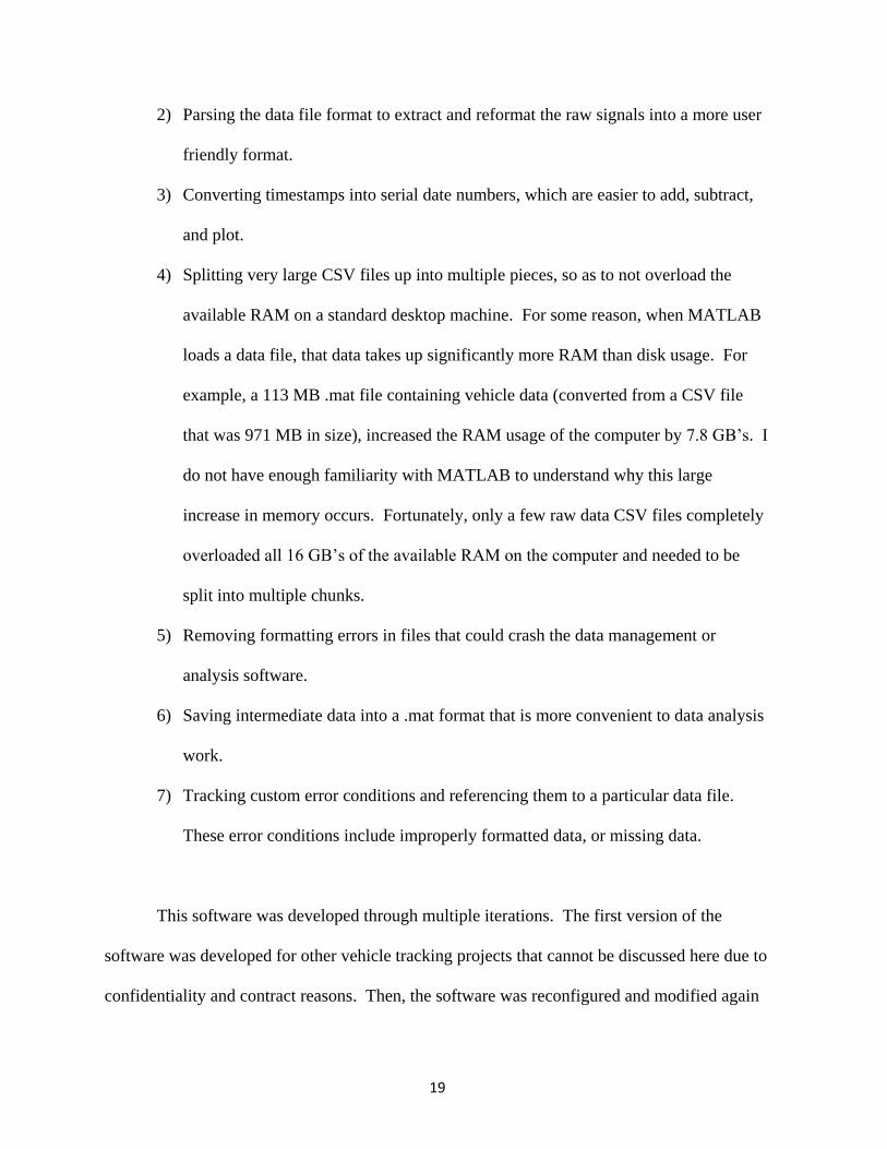
2) Parsing the data file format to extract and reformat the raw signals into a more user

friendly format.

3) Converting timestamps into serial date numbers, which are easier to add, subtract,

and plot.

4) Splitting very large CSV files up into multiple pieces, so as to not overload the

available RAM on a standard desktop machine. For some reason, when MATLAB

loads a data file, that data takes up significantly more RAM than disk usage. For

example, a 113 MB .mat file containing vehicle data (converted from a CSV file

that was 971 MB in size), increased the RAM usage of the computer by 7.8 GB’s. I

do not have enough familiarity with MATLAB to understand why this large

increase in memory occurs. Fortunately, only a few raw data CSV files completely

overloaded all 16 GB’s of the available RAM on the computer and needed to be

split into multiple chunks.

5) Removing formatting errors in files that could crash the data management or

analysis software.

6) Saving intermediate data into a .mat format that is more convenient to data analysis

work.

7) Tracking custom error conditions and referencing them to a particular data file.

These error conditions include improperly formatted data, or missing data.

This software was developed through multiple iterations. The first version of the

software was developed for other vehicle tracking projects that cannot be discussed here due to

confidentiality and contract reasons. Then, the software was reconfigured and modified again

20

to run on both the Odyne and Via Truck data from EPRI. Numerous improvements were

implemented during each of the software iterations. This thesis only focuses on the final

version of the software that I developed. For the Electric Vehicle Symposium 29 (EVS29)

conference paper, Zachary Wilkins further modified the framework described in this document

to better suit his needs, but his work on the data management framework will not be heavily

described in this document. In addition, much of this framework was rewritten by Mike Reid

for the analysis work presented in Section 5 and Subsection 5.2 and it served as a foundation to

develop new versions of the analysis software.

There are two main components in this framework that run as separate scripts. The first

is a data extraction and parsing framework which runs through the script titled

Extract_all_Truck_data_v1.m. This first component was responsible for parsing the raw CSV

data files, reformatting the data, removing any obvious formatting errors, and then resaving the

data into a .mat file format. By resaving the data, subsequent data analysis would not have to

rerun this initial data parsing and validation step. All data analysis can be run directly out of

the .mat files.

The second main component of the framework is where scientific data analysis code

can be added later, which runs through the script titled Analyze_all_truck_data_v1.m. The raw

code is mostly just a framework that additional analysis code can be added into. This empty

framework is responsible for keeping track of all the data files to be processed and then passing

the file names to a sub-function where each data file is loaded and processed independently.

The framework also includes a custom error tracking system, where the future data analysis

code can flag custom error conditions when it is processing certain data files. These error

codes are then summarized for all data files at the end of the script run. Finally, the framework

21

can reduce each data file into a single Excel spreadsheet row, so information such as fuel

consumption, total distance traveled, etc. can be compiled by vehicle. All the spreadsheet rows

are then combined into a single Excel spreadsheet. The idea was that fleet-level analysis could

be performed on this output spreadsheet using Excel and no additional MATLAB development

would be needed to combine vehicle results into fleet results.

The below flowchart summarizes the data processing flow inside of this framework as

the data moves through the data extraction and analysis software modules:

Figure 2.1 – High-Level Data Processing Flow between Modules of the MATLAB Data

Management Framework

2.2 Details of the Data Extraction and Parsing Component

This section describes in more detail how the data extraction script works for the EPRI

Commercial Truck data.

Raw CSV data files

Data Extraction

Script:

Parses raw CSV files, reformats, validates, and resaves into .mat format

Data Analysis Script:

Empty framework into

which data analysis code can be added.

Results:

Summarized data for each vehicle data file in Excel

Spreadsheet format.

22

The Extract_all_Truck_data_v1.m data extraction script is a preprocessing step for the

Analyze_all_truck_data_v1.m script, which is explained next in Subsection 2.3. The goal of

the Extract_all_Truck_data_v1.m script is to perform data reformatting, data validation, and

save the data into a .mat format that is faster to load and process during data analysis. This

way, when the data analysis needs to be run multiple times for development and debugging, all

of this up front work will not need to be rerun.

Data validation is built into the software, to identify any corrupt data. For example, the

software checks that each line of CSV data has the proper number of delimiters, each file has a

proper header, and after the data is parsed from the CSV file it again checks the size of the data

to ensure that all of the data was properly imported. If there are corrupt lines of data, the

process will attempt to remove these lines so the non-corrupt lines can still be used. When

corrupt data is encountered, an error code will be generated, a summary of errors will be

displayed in the command window when the script completes, and the command window

output can be continuously appended into a text file (if runlog is activated).

The code is structured into two main levels. The highest level script tracks all of the

data files to be processed and collects error codes, while the

epri_truck_data_file_extract_fcn_v1.m sub-function, which is called from the high-level script,

processes individual data files. Multiple .mat data files may be created for a single CSV file if

the data size is too large so available RAM is not overloaded. This sub-function also contains

data validation tools that will prevent the loading of corrupt CSV data. In addition, if the

function header is commented out and the input variables are defined explicitly in the function

(there is a commented out section of code just for this), it can be run as a script for testing

purposes.

23

All of the parameters needed to adjust the performance of the

Extract_all_Truck_data_v1.m are in a Controlling Variables section near the top of the script.

Comments provide additional explanation of these variables. For example, these variables

define which directories data should be read from and saved to, and define switches that can

turn on and off certain script functions.

%% CONTROLLING VARIABLES - Use the controlling values to adjust the performance of the script. % This section is used to initialize the script, point it towards the % appropriate file directories, etc. % % Be sure to save this script after changes if it will be launched by % another script. % SET CURRENT DIRECTORY cd('T:\projects\EPRI2014\MATLAB\Odyne Data and Analysis') % Windows % cd('/net/projects/data/projects/EPRI2014/MATLAB') ;% Linux Server % RUN PROFILES. % Each run profile is a branch of an if statement, and the control_profile % variable controls with branch is run to initialize the script. % This allows the user to quickly switch between different commonly used run settings. % Additional elseif statements can be added to create new run profiles if % needed. % % Values: % 1 - Actual Data (Test) % 2 - Data Validation Test control_profile = 2 ; % ------------------------------------------------------------------------------- % PROFILE 1 - ACTUAL DATA VIA TEST if control_profile == 1; % DIRECTORY TO LOAD - CSV DATA control_filedir_load = 'T:\projects\EPRI2014\MATLAB\Odyne Data and Analysis\Data\CSV\Via_Join_Test/' ; % Test Data % Location of files to be extracted relative to CD. Be sure to include \ at end of string. % DIRECTORY TO SAVE EXTRACTED MAT DATA control_filedir_save = 'T:\projects\EPRI2014\MATLAB\Odyne Data and Analysis\Data\MAT\Via_Join_Test_MAT/' ; % Test Data % Location of where to save processed .mat file relative to CD. Be sure to include \ at end of string. % DO YOU WANT TO CREATE A RUNLOG FOR TROUBLESHOOTING? % This is recommended when large amounts of data are being processed to

24

% help troubleshoot a system crash, or verify the accuracy of results. It also provides documentation of the % conversion process. control_create_runlog = 1 ; % 0 - do not create a runlog when script executes. % 1 - save runlog in designated location. control_runlog_nameandloc = [control_filedir_save 'Extract_all_Truck_data_v1_runlog' ] ; % Test Data % Specify runlog file name and location in relation to the CD as a % text string. Note that script start time and .txt will be appended % onto the end of the runlog file name specified. % DEFINE MAX NUMBER OF DATA LINES PER .MAT FILE control_max_number_of_datalines = 1250000 ; % This value defines the maximum number of data lines that can be loaded and saved % into a .mat file at a time. This is to prevent RAM from being maxed % out and crashing the machine when very large data files need to be % processed, so they can be processed on a regular computer. CSV files % with more data lines than the maximum will automatically be split up % into multiple .mat files. % ------------------------------------------------------------------------------- % PROFILE 2 - DATA VALIDATION TEST elseif control_profile == 2; % DIRECTORY TO LOAD - CSV DATA

Figure 2.2 - Controlling Variables Section of Code

The first section of MATLAB code (Figure 2.2 above) shows the controlling variables

section. Since the user may have multiple configurations that they frequently run, such as a

configuration for testing and a configuration for actual data analysis, different profiles can be

created to save these settings so they do not need to be constantly adjusted. To create a new

profile, copy all of the variables from an existing profile and put the copy into a new branch of

the if-else statement. The control_profile variable is just a number that tells the script which

section of the if-statement to execute for a given configuration. The goal of this system is to

make it very easy to switch between different settings to reduce setup errors.

25

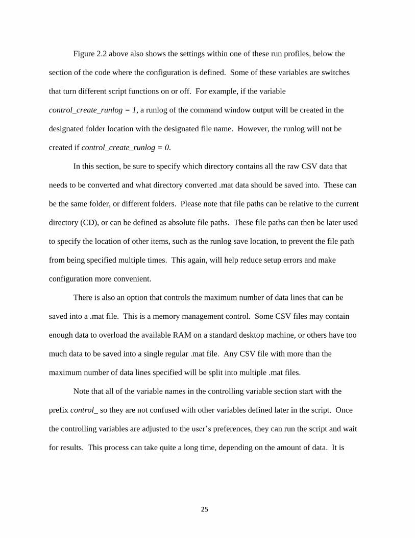
Figure 2.2 above also shows the settings within one of these run profiles, below the

section of the code where the configuration is defined. Some of these variables are switches

that turn different script functions on or off. For example, if the variable

control_create_runlog = 1, a runlog of the command window output will be created in the

designated folder location with the designated file name. However, the runlog will not be

created if control_create_runlog = 0.

In this section, be sure to specify which directory contains all the raw CSV data that

needs to be converted and what directory converted .mat data should be saved into. These can

be the same folder, or different folders. Please note that file paths can be relative to the current

directory (CD), or can be defined as absolute file paths. These file paths can then be later used

to specify the location of other items, such as the runlog save location, to prevent the file path

from being specified multiple times. This again, will help reduce setup errors and make

configuration more convenient.

There is also an option that controls the maximum number of data lines that can be

saved into a .mat file. This is a memory management control. Some CSV files may contain

enough data to overload the available RAM on a standard desktop machine, or others have too

much data to be saved into a single regular .mat file. Any CSV file with more than the

maximum number of data lines specified will be split into multiple .mat files.

Note that all of the variable names in the controlling variable section start with the

prefix control_ so they are not confused with other variables defined later in the script. Once

the controlling variables are adjusted to the user’s preferences, they can run the script and wait

for results. This process can take quite a long time, depending on the amount of data. It is

26

recommended to start running the process overnight, and even then it still may not be finished

by the next morning.

The sub-function that converts individual CSV files to .mat data has the following

format (shown below in Figure 2.3):

[errorcode critical_fileerror] =

epri_truck_data_file_extract_fcn_v1(filedir_load,

filename_load, filedir_save, filename_save, max_number_of_datalines)

Figure 2.3 - Format of the Data Extraction Sub-Function for Individual CSV Files

Function output is optional and only indicates if an error was encountered. While the

function is running, information will be printed into the command window as well so it may

not be necessary to collect the error code output. The errorcode output variable contains

numbers that correspond to specific error conditions. This can be a single number, or an array

of numbers for multiple error conditions. Note that an errorcode of 0 indicates that no errors

occurred. The critical_fileerror output variable will always be a single value that indicates the

severity of all the error conditions encountered and it helps define what actions should be taken

by the higher level script. A critical_fileerror of 0 indicates that the errorcode is more of an

advisory to the user and no automated response is needed. A critical_fileerror of 1 indicates

that some of the .mat data files corresponding to the CSV file may be deleted due to corrupt

data. A critical_fileerror of 2 indicates that no .mat data should be saved for the vehicle and

any .mat data saved previously should be deleted (note, the functionality to delete data files

may not be in the extract data script for the medium duty truck data as critical_fileerror of 2 is

not used in this script). critical_fileerror = 2 is the most severe.

27

Additional error codes can be added into the epri_truck_data_file_extract_fcn_v1

function if the software needs further development and compiled in the higher level

Extract_all_Truck_data_v1.m script. The process to add new error conditions is the same as

the process used in the analyze data script, so read Subsection 2.3 which is next about the

analyze data script for more details.

2.3 Details of the Data Analysis Framework Component

After the data is transferred into .mat files by the data extraction script described in the

previous Subsection 2.2, the next step is to analyze the data. This Subsection describes a

framework that loads and manages the .mat files, and tracks error codes, into which additional

data analysis code can be easily added. After loading these .mat files, the

Analyze_all_truck_data_v1.m script will compile results from each individual .mat file into an

Excel spreadsheet where fleet summary statistics can be compiled. A process to report error

codes is also built into the script, so data files that have corrupt data, or do not process

correctly, can be identified. Overall, this script can load and keep track of multiple data files,

so fleet wide analysis can be performed.

The structure of the data analysis script is similar to the data extraction script, as the

highest level of the script tracks and manages all of the data files and then a sub-function

named epri_truck_data_file_analyze_fcn_v1.m loads each individual file and performs the

analysis on the data within it. Much of the code from the data extraction script was copied to

create the data analysis script.

The highest level Analyze_all_truck_data_v1.m script loads multiple .mat vehicle files

in a directory for analysis. The script will compile a summary of the analysis output for each

28

vehicle into an Excel Spreadsheet. Results from the data analysis can also be saved into a .mat

file, where the results are stored into a cell array that mimics the spreadsheet format. This

script is a framework that future data analysis can be added into, although some simple sample

data analysis, such as a count of the number of data points in the file, is included in the empty

framework to demonstrate how the script works.

The epri_truck_data_file_analyze_fcn_v1.m sub-function analyses data in a single .mat

vehicle file and outputs the results. Additional analysis code can be added into the body of this

function in the future. The function is automatically invoked from the

Analyze_all_truck_data_v1.m script, but it can also be run through the command window to

analyze a single data file. In addition, if the function header is commented out and the input

variables are defined explicitly in the function (there is a commented out section of code just

for this), the function can be run as a script for testing purposes.

2.3.1 Instructions for Running the Data Analysis Framework

All of the parameters needed to adjust the performance of the

Analyze_all_truck_data_v1.m script are in a Controlling Variables section near the top of the

script. Comments provide additional explanation of these variables. This controlling variables

section is shown below (in Figure 2.4).

29

%% CONTROLLING VARIABLES - Use the controlling values to adjust the performance of the script. % This section is used to initialize the script, point it towards the % appropriate file directories, etc. % % Be sure to save this script after changes if it will be launched by % another script. % SET CURRENT DIRECTORY cd('T:\projects\EPRI2014\MATLAB\Odyne Data and Analysis') % Windows % cd('/net/projects/data/projects/EPRI2014/MATLAB') % Linux Server % RUN PROFILES. % Each run profile is a branch of an if statement, and the control_profile % variable controls with branch is run to initialize the script. % This allows the user to quickly switch between different commonly used run settings. % Additional elseif statements can be added to create new run profiles if % needed. % % Values: % 1 - Data Validation Test % 2 - Actual Data Odyne % 3 - Actual Data Via control_profile = 2 ; % ------------------------------------------------------------------------------- % PROFILE 1 - TEST DATA if control_profile == 1; % DIRECTORY TO LOAD PREFERENCES - MAT DATA control_filedir_load = 'T:\projects\EPRI2014\MATLAB\Odyne Data and Analysis\Data\MAT\Data_Validation_Test_MAT\' ; % Test folder location % Location of .mat files to be analyzed relative to CD. Be sure to include \ at end of string. % DIRECTORY TO SAVE ANALYSIS RESULTS control_results_save = 'T:\projects\EPRI2014\MATLAB\Odyne Data and Analysis\Data\Analysis_Results\Data_Validation_Test_Results\' ; % Location of directory where all data analysis results will be saved. % DO YOU WANT TO CREATE A RUNLOG FOR TROUBLESHOOTING? % This is recommended when large amounts of data are being processed to % help troubleshoot a system crash, or verify the accuracy of results. It also provides documentation of the % conversion process. control_create_runlog = 1 ; % 0 - do not create a runlog when script executes. % 1 - save runlog in designated location. control_runlog_nameandloc = [control_results_save 'Analyze_all_truck_data_v1_runlog - Test' ] ; % Test data % Specify runlog file name and location in relation to the CD as a % text string. Note that script start time and .txt will be appended % onto the end of the runlog file name specified.

30

% DO YOU WANT TO COMPILE A LIST OF ALL VEHICLES AND THEIR RESULTS INTO AN % EXCEL SPREADSHEET? control_create_spreadsheet = 1 ; % 0 - do not create an excel spreadsheet that summarizes individual % vehicle results at the end of the script % 1 - Compile a summary of vehicle results into a spreadsheet at % the end of the script. control_nameandloc_create_spreadsheet = [control_results_save 'Analyze_all_truck_data_v1_spreadsheet_result_summary - test' ] ; % Test data % Specify spreadsheet name and location in relation to the CD as a % text string. Note that .xls will be automatically included on the % end of the file name and does not need to be included in the text % string. % NOTE: Existing summary spreadsheets can be overwritten, but be sure % the summary spreadsheet is closed before running this script. % DO YOU WANT TO USE A EXCEL VIN LIST SPREADSHEET TO MANUALLY FILTER OUT % VEHICLE FILES FROM THE DATA ANALYSIS? % This spreadsheet is a list of all VIN numbers, and it can be used to % check which vin numbers should not be processed with an 'x'. % Note: First column of the spreadsheet should contain a column that has % either values of "x" or are blank. The second column should contain % vehicle vin numbers. VIN numbers with X will be skipped during data analysis. % Any additional columns will be ignored by this matlab script, but can be % included if the information is helpful in the spreadsheet. % "x" is not case sensitive and can have leading or trailing spaces. This % data should start on the second row of the spreadsheet. It will be % assumed that the first row is a header. control_load_vinlist_spreadsheet = 0 ; % 1 - Load a spreadsheet containing a list of vin numbers. VIN % numbers marked with "x" will be excluded from the analysis. % 0 -Do not load a spreadsheet containing a list of vin numbers. control_vinlist_spreadsheet_nameandloc = [ control_filedir_load 'List_of_trucks-test.xlsx' ] ; % Test Data % Specify the name and location relative to the CD where the % spreadsheet containing a list of VIN numbers is located. Be sure % to include .xls or .xlsx at the end of the spreadsheet name. % DO YOU WANT TO AUTOMATICALLY SAVE DATA ANALYSIS RESULTS INTO A .MAT FILE? control_save_results_as_mat = 1 ; % 1 - Save final workspace as .mat file after data analysis completes. % 0 - Do not save final workspace as .mat file. control_matresults_nameandloc = [control_results_save 'Analyze_all_truck_data_v1_mat_datafile.mat' ] ; %Test Data % filepath and filename relative to the CD where the .mat file of results should be % saved. Variable should be string. Be sure to include .mat at the end of the % string. % DO YOU WANT TO CREATE PLOTS AND FIGURES DURING THE DATA ANALYSIS PROCESS? control_save_figs = 0 ; % 1 - Save figures for each vehicle file in designated location. % 0 - Do not save any figures from data analysis. control_fig_save_loc = [control_results_save 'Figs\' ] ; % Test Data

31

% filepath relative to CD where .fig files genereated in analysis % should be saved. Variable should be a string. Be sure to include % a \ at the end of the string. % ------------------------------------------------------------------------------- % PROFILE 2 - FULL DATA SET FOR ODYNE elseif control_profile == 2; % DIRECTORY TO LOAD PREFERENCES - MAT DATA

Figure 2.4 – Run Profile Settings in the Controlling Variables Section of Code

The first section of MATLAB code (in Figure 2.4 above) shows the control profile

section. Since the user may have multiple configurations that they frequently run, such as a

configuration for testing and a configuration for the full data analysis, different profiles can be

created to save these settings so they do not need to be constantly adjusted. To create a new

profile, copy all of the variables from an existing profile and put the copy into a new branch of

the if-else statement. The control_profile variable is just a number that tells the script which

section of the if-statement to execute for a given configuration. The goal of this system is to

make it very easy to switch between different settings to reduce setup errors.

Figure 2.4 above also shows the settings within one of these run profiles. Some of

these variables are switches that turn different script functions on or off. For example, if the

variable control_create_runlog = 1, a runlog of the command window output will be created in

the designated folder location with the designated file name. However, the runlog will not be

created if control_create_runlog = 0.

In this section, be sure to specify which directory contains the .mat data files that need

to be converted and where the final analysis results should be saved. Please note that file paths

can be relative to the current directory (CD), or can be defined as absolute file paths. These

file paths can then be later used to specify the location of other items such as the runlog save

32

location, spreadsheet result save location, and figure save location. By concatenating these

general-high level file paths to create lower level folder structures, this prevents the file path

from being typed by the user multiple times to reduce setup errors and make configuration

more convenient. Basically, the setup is similar to the data extraction function, but with more

options.

A major difference between this script and the extract all data script is that spreadsheets

can be imported and exported. If control_create_spreadsheet = 1, all of the data analysis

results will be exported into an Excel spreadsheet and saved in the designated location. The

data analysis results for each vehicle are listed in the spreadsheet. Note that cell dimensions

and formatting may need to be adjusted within the Excel interface after the spreadsheet is

exported.

If there are multiple .mat files for a single vehicle file, there will be multiple rows of

data output for that vehicle. The easiest way to combine results into a table that shows the

cumulative results for a single vehicle on one line is to use a pivot table in Excel. I did not

want to spend weeks programming MATLAB to do this when the capability was already built

into Excel.

If control_load_vinlist_spreadsheet = 1, a control spreadsheet will be imported to help

manually filter out individual vehicles. In the control spreadsheet, VIN numbers with an ‘X’

marked next to them will not be analyzed. The X’s should be in the first column of the

spreadsheet and the VIN numbers should be in the 2nd column of the spreadsheet. Any other

columns are extra information and will be ignored by the Analyze_all_truck_data_v1.m script.

Note that ‘X’ is not case sensitive and can have leading and trailing blank spaces. It

will also be assumed that the first row of the spreadsheet is a header and VIN numbers should

33

start on the second row. Be sure that the VIN list spreadsheet is formatted exactly as specified.

Also note that a warning will be produced if the VIN number in the spreadsheet does not match

the VIN number in the vehicle .mat file. Each vehicle data file should contain a VIN number

before the first underscore ( _ ) in the file name in this implementation of the framework.

Another option that can be selected is to automatically save the final workspace as a

.mat file when the script completes. This offers an alternative format from which vehicle

summary information can be analyzed and provides a data backup in case an Excel spreadsheet

cannot be exported. If this option is turned on, the name and location of where the .mat file

should be saved needs to be specified under controlling variables.

Finally, the last option allows custom figures and charts to be saved for each .mat file.

The data analyst is responsible for programming the charts they want into the MATLAB data

analysis framework, so this feature just creates an easy framework that can be turned on to

manage these graphs. These can help the user visualize the data for individual vehicle files

after a data analysis run and can also help spot problems in the dataset. However, a very large

number of graphs can be generated and this slows down the process, so the user may want to

turn off automatic figure generation in some situations.

Note that all of the variable names in the controlling variable section start with the

prefix control_ so they are not confused with the other variables that are defined later in the

script. Overall, once the controlling variables are adjusted to the user’s preference they can run

the script and wait for results. This process can take quite a long time, depending on the

amount of data.

This function can be used individually to analyze a single data file. It has the following

format (shown below in Figure 2.5):

34

[spreadsheet_export_headers spreadsheet_export_row errorcode critical_fileerror]

= epri_truck_data_file_analyze_fcn_v1(control_filedir_load, filename_load,

control_save_figs, control_fig_save_loc)

Figure 2.5 - Format of the Data Extraction Sub-Function for Individual .mat Files

Like the extract all data script, the analyze data script contains the same error code

tracking system. The errorcode output variable contains numbers that correspond to specific

error conditions. This can be a single number, or an array of numbers for multiple error

conditions. Note that an error code of 0 indicates that no errors occurred. The

critical_fileerror output variable will always be a single value that indicates the severity of all

of the error conditions encountered and it helps define what actions should be taken by the

higher level script. A critical_fileerror of 0 indicates that the errorcode is more of an advisory

to the user and no automated response is needed. A critical_fileerror of 1 indicates that some

of the .mat data files corresponding to the CSV file may be deleted due to corrupt data. A

critical_fileerror of 2 indicates that no results from .mat data should be saved for the vehicle

and any analysis results previously saved should be deleted. critical_fileerror = 2 is the most

severe.

The other two output variables contain data analysis results in the form of a cell array

row. spreadsheet_export_row contains all output values concatenated into a horizontal cell

array. This will eventually form a row of data output in the Excel spreadsheet.

spreadsheet_export_headers contains text headers that correspond to the values in the

spreadsheet_export_row. The header cell array should be the same size as the row cell array,

or else MATLAB will crash.

A controlling variables section also exists in the epri_truck_data_file_analyze_fcn_v1

sub-function as well as the main script, where key variables that affect the performance of data

35

analysis for an individual vehicle can be controlled and tuned. This is shown below in Figure

2.6.

Currently, the only value in this section is min_datapoints, which controls Error Code

1. This prevents the function from processing any data files with less than the specified

number of data points. Additional controlling variables can be added to this section if more

complex analysis is added into the data script. For example, maybe there are certain cutoff

values that control data filtering or separation steps.

%% Controlling Variables % Use these variables to tune the performance of the analysis function. % Minimum acceptable number of data points that can be in a .mat file to % process the file. This includes all bus message values. min_datapoints = 300 ; %% Begin Script - Initialize Workspace

Figure 2.6 - Controlling Variables Section in Data File Analyze Function

Since this code is only a data management framework that loads file data and produces

basic data statistics, additional data analysis will need to be added into it in the future. Here

are the steps that need to happen when an additional data output variable and the corresponding

logic are added into the function.

2.3.2 Instructions to Add Data Analysis Code Into the Data Analysis Framework

Note that absolutely no modifications need to be made to the higher level

Analyze_all_truck_data_v1.m data script for new data output to be added.

36

Step 1: Add additional code to produce a new data output in the commented section of code

shown below (Figure 2.7).

The below section of code is where the actual data analysis can be added.

%% DATA ANALYSIS - Add additional data analysis code here. % Create additional sections as needed. % When creating new output variables, be sure to: % > Initialize these new output variables in the initialize variables section where indicated % > Concatenate the new output variables into the spreadsheet_export_row % cell array, which will be sent to the higher level script and compiled % into an excel spreadsheet. Be sure to define new headers that correspond % to the indecies in spreadsheet_export_row in spreadsheet_export_headers % as well. % > Define the new output variables in the function comments section at % the top of the script. % > Add additional print screen output at the end of this script if % desired, to print results to the screen.

Figure 2.7 - Step 1 of Adding Additional Data Analysis

Step 2: Be sure to initialize any new output variables generated in Step 1 in the “Begin Script

– Initialize Workspace” section of code shown below (Figure 2.8).

If an error code is produced, this ensures that a generic output value will still be

produced. This will help prevent MATLAB exceptions that could crash the process.

37

% Initialize Generic Data Output Variables datapointcount = []; % Count of data points in .mat file firstdatapoint_serialdate = 0; % first/earliest serial date number in .mat file firstdatapoint_timestamp = {''}; % first/earliest serial date number in .mat file converted to time stamp lastdatapoint_serialdate = 0; % last/ latest serial date number in .mat file lastdatapoint_timestamp = {''}; % last/ latest serial date number in .mat file converted to time stamp vin = 0; % Vin number, extracted from data file name filenum = 0; % File number, extracted from data file name. There can be multiple .mat files for a single vin. filecount = 0; % Total number of .mat files for a single vin. This is extracted from the data filename. % Initialize specific data output Variable % ADD VARIABLE INITIALIZATION FOR FUTURE DATA OUTPUT HERE

Figure 2.8 - Step 2 of Adding Additional Data Analysis

Step 3: Concatenate the new data output variables into the spreadsheet_export_row cell

array at the bottom of the script. Define new spreadsheet headers that correspond to the

spreadsheet row in the spreadsheet_export_headers cell array.

These spreadsheet variables are the function outputs, which will be compiled into an

Excel spreadsheet. Note that the variables spreadsheet_export_row and

spreadsheet_export_headers are aligned, to ensure that spreadsheet headers will correspond to

the correct data in the Excel spreadsheet. In the below example, there was not enough

horizontal space to show the sample code in this format. In the MATLAB software, use the

horizontal scroll bar to see the full length of the values in these vectors. The section of code

where this is defined is shown below (in Figure 2.9).

38

% Horizontally concatenate all output variables and header labels into cell % arrays. spreadsheet_export_array must be cell array. Excel spreadsheet % columns will be in the order of data concatenation. spreadsheet_export_headers = { 'File Name', 'VIN', 'File Number', 'Number of Data Files for VIN', 'Error Code Output', 'Severity of Error Code', 'Number of Data Points in File', 'First Data Point Collected at:', 'Last Data Point Collected at:', 'First Data Point Collected at (MATLAB serial date):', 'Last Data Point Collected at (MATLAB serial date):' }; spreadsheet_export_row = { filename_load vin filenum filecount errorcode_string critical_fileerror datapointcount firstdatapoint_timestamp lastdatapoint_timestamp firstdatapoint_serialdate lastdatapoint_serialdate }; % FOR FUTURE DEVELOPMENT, BE SURE TO CONCATENATE NEW VARIABLES AND % HEADERS TOGETHER HERE TO COLLECT RESULTS IN SPREADSHEET.

Figure 2.9 – Step 3 of Adding Additional Data Analysis

Step 4 – Optional: Add new summary statistics print screen in “End of Function Display”

section of code (shown in Figure 2.10).

This will print the data analysis results to the command window, which can then be

saved into the overall runlog output. This output is redundant and harder to reference than

Excel spreadsheet data, but it could be useful depending on user preferences.

%% End of Function Display if critical_fileerror == 0 % Output if no critical Error fprintf('--------------------------------------------------------\n') fprintf('\nData was successfully analyzed from the file:\n\t%s\n\n', fileloc) % Summarize selected Output Variables in Print Screen fprintf('Summary of output vehicle statistics from analysis:\n\n') fprintf('\t%d - datapointcount - Total Number of Data Points in Vehicle File. \n', datapointcount) fprintf('\t%s - firstdatapoint_timestamp - Date/time when the first/earliest data point in vehicle file was collected.\n', firstdatapoint_timestamp) fprintf('\t%s - lastdatapoint_timestamp - Date/time when the last/latest data point in vehicle file was collected.\n\n', lastdatapoint_timestamp) % FOR FUTURE DEVELOPMENT, ADD ADDITIONAL PRINT SCREEN OUTPUT HERE FOR % ANY ADDITIONAL OUTPUT VARIABLES ADDED, IF DESIRED. end

Figure 2.10 – Step 4 of Adding Additional Data Analysis

39

Step 5 – Optional but Recommended: Update output variable description in the

comments at the beginning of the function (shown in Figure 2.11) to include new output

variable.

This will help document what the outputs are for future reference.

% > spreadsheet_export_row - Cell array that contains all output % variables. Be sure to include a description of all output variables % that are compiled into this cell array below: % % General Output - applicable to any data analysis: % > filename_load - This input variable is also provided as an output % for reference % > vin - VIN number extracted from file name, for reference % > filenum - .mat file number, that indicates which .mat file is % beign processed if there are multiple .mat files per vehicle. % This is extracted from the .mat filename % > filecount - Total number of mat files for a vehicle. This is % extracted from the .mat file name. % > errorcode_string - Text string of all error codes produced by the % data analysis, for reference in the Excel Spreadsheet. % > critical_fileerror - copy of critical fileerror output to the % function, for reference in the excel spreadsheet. % > datapointcount - The total number of data points in the vehicle file (all % bus messages). % > firstdatapoint_timestamp - Time stamp corresponding to first/ earliest data point collected. % > lastdatapoint_timestamp - Time stamp corresponding to last/ latest data point collected. % > firstdatapoint_serialdate = firstdatapoint_timestamp as MATLAB serial date number. % > lastdatapoint_serialdate = lastdatapoint_timestamp as MATLAB serial date number. % % Specific output to data analysis: % Add a description of new specific data output variables here.

Figure 2.11 – Step 5 of Adding Additional Data Analysis

If a new error code needs to be added to the shell script and function, follow these steps.

40

Step 1: Write code that defines a new unique value for the variable errorcode in the

epri_truck_data_file_analyze_fcn_v1.m function if some error condition occurs.

A section of code to demonstrate this is not provided, because this could occur at many

different points in the function code.

When an error code is defined, be sure to update the variable errorcode to the new

value, or if errorcode already has previous errors, concatenate the new variable vertically onto

the end of the existing values if multiple error codes should be reported. In addition

critical_fileerror may need to be updated as well, so the script can take some action. Be

careful to not downgrade the severity of critical_fileerror if a more severe error code was

encountered previously. It is the programmer’s responsibility to ensure the data analysis code

produces the proper errorcode and critical_fileerror outputs for all possible error conditions.

If statements can be used around subsequent sections of code to prevent execution if an error

code has been encountered, or a function return statement can be used. The user will have to

design a system to ensure proper errorcode reporting.

It may be a good idea to add some print screen output into the function when the error

code is encountered and defined, such as:

errorcode = 1; % Too Few Data Points - All bus messages. critical_fileerror = 1; fprintf(['ERROR CODE 1: There are too few data points in this file

for data to be analyzed.' ... '\nThe file only has %d data points.\nThe File must contain at

least %d data points.\n\n'], ... length(time_days_serialnum), min_datapoints)

Figure 2.12 – Sample Error Code Output Code

It is recommended to add two new lines ‘\n’ onto the end of the print screen output to

maintain spacing.

41

Step 2 – Optional but Recommended: Add a new error code description into the output

variable description for errorcode in the comments at the beginning of the function.

This will help document what the new error code value means for future reference.

% OUTPUTS ARE: % > errorcode - Numeric values corresponding to different error conditions: % 0 - No error % 1 - Too Few Data Points - All bus messages. % % errorcode can also contain multiple error codes for a single file, if % multiple errors are encountered. If this occurs, errorcode should be % a vertical vector which contains all the error codes produced. It is % the programmers responsibility to ensure that errorcode always % produces the appropriate output when modifying this script.

Figure 2.13 – Step 2 of Adding Additional Error Codes

Step 3: Script Changes – Add new print screen output into the higher level

Analyze_all_truck_data_v1.m script that lists which files produced the error code at the end of

script execution. This will print the errorcodes produced by all .mat files into a summarized

list.

Match the format of existing error code print screen outputs. The value of errorcode

outputted by the function needs to be updated in the following highlighted locations. This is

critical to ensure proper output.

The example below (in Figure 2.14) is an error code which does not exist in the current

script format, but provides an illustrative example. Also, update the print screen description so

an appropriate message is displayed.

42

% Display all Error Code 3 files if length(find(track_errorcodes(:, 2)==3)) > 0

fprintf(['Files Producing ERROR CODE 3: Vehicle file contains multiple VIN numbers in discrete value data. \nThere' ...

' should only be 1 VIN number per vehicle file.\nNo data from this VIN number will be saved in analysis results.\n\n'])

% Display the names of all files that produced error code 3. fprintf('\t%s\n',

data_directory_filenamelist_raw(track_errorcodes(find(track_errorcodes(:, 2)==3), 1)).name)

fprintf('\n') end

Figure 2.14 – Step 3 of Adding Additional Error Codes

Additional actions do not need to be taken to compile error codes. This will be done

automatically when any error code is detected. Error codes are tracked in the variable

track_errorcodes in the Analyze_all_truck_data script, where the first column corresponds to

an index in the data_directory_filenamelist_raw.name structure that lists each vehicle file, the

second column contains the actual error code, and the third column corresponds to the value of

critical_fileerror to define severity.

2.4 Future Work That Could Improve the MATLAB Big Data Analysis Framework

Although the data analysis framework was used successfully, there is always room for

additional improvement. This section outlines future work that could be implemented to make

the data analysis framework even more robust and useful to future projects. There is a huge

advantage to having efficient, clean, and robust code. Although it takes longer to develop, it

can prevent major hassles down the road when it is finally implemented and used. Here are

some suggested areas where the described software can be improved:

1) Parallel processing could be implemented into the data analysis framework using

MATLAB ’s parallel computing toolbox [34] and it could be run on a computer

cluster. Currently the code runs on a single core and can take days to process all of

the data. However, since each data file is processed independently, in theory it

43

should be relatively easy to run the analysis in parallel on a computer cluster. It is

likely that the for loops would need to be changed into parfor loops and distributed

arrays would possibly have to be used to collect output. It is also possible to run

MATLAB on a Hadoop Cluster [35].

2) Reduce hard coded values that control the data extraction CSV input format. It

should be easy to modify the data extraction script to accept different CSV formats,

but there is no centralized system that controls the input file format. All of the

values related to format should be collected into one location, similar to the

controlling variables section. Maybe these could be grouped together into a

separate data format definition script that launches from the main script.

3) MATLAB structures could be used to group similar variables together.

4) A Try / Catch statement could be implemented around the section that loads data

files, in case the file system becomes unavailable. This could also be placed inside

of a loop, so the system will continue to try and load the data until it becomes

available. Occasionally, there were issues where a network issue would make our

folder structure containing our dataset unavailable.

44

SECTION 3

INITIAL FEASIBILITY ASSESSMENT OF USING THE EPRI VEHICLE TRACKING

DATA TO ANSWER POTENTIAL RESEARCH QUESTIONS

3.1 Introduction to the Feasibility Assessment

A feasibility assessment was conducted in the Fall of 2014 on some of the preliminary

data to better understand what kinds of questions could be answered. The work in this section

laid the foundation for this future work. Below is a list of the questions that were evaluated for

feasibility. Not all of these questions were analyzed as many are very complex data analysis

problems, so this section just outlines some theoretical approaches that could be used to

attempt to answer the questions and what CAN signals might be needed. However, it was a

good initial exercise to identify what questions might be the most feasible and valuable to

answer, and what approach might be taken. This provided a guide to help determine which

problems were to be analyzed later in this thesis. Here is a list of the questions that were

evaluated. Questions in italic-bold text are examined and analyzed in some form later in this

thesis.

How efficient are the vehicles?

What is the effective range of the vehicles?

How much energy do the vehicles use?

What kinds of utility load shapes do we see when the vehicle is charging?

What is the Utility Factor (UF) for the Vehicles?

How does HVAC affect vehicle performance?

How often were the vehicles charged over a certain period of time?

45

How long did the vehicles go between charges? How long were they charging?

How often was the vehicle driven? In general, how far was a trip?

Did vehicles mostly travel between a handful of “unique” places, or were driving

patterns more scattered? Were most trips between a couple of locations?

Define some kind of assessment of vehicle performance (perhaps a combination of

a couple of things such as efficiency or use depleting and charging of the battery).

Show a comparison of the different vehicles, perhaps highlighting why they are

or are not different.

How much energy is recovered by regenerative braking?

How do climate and weather conditions affect vehicle performance and driving

patterns?

It is important to keep in mind that the information presented in this section only

provides an initial feasibility assessment. If more data analysis and feasibility assessment were

performed, more information would become available and feasibility assessments and analysis

approaches may change. Unexpected problems that cannot be anticipated could still be

encountered. However, this section also provides an important foundation to identify which

questions make the most sense to answer and provides a starting point to answer those

questions.

The remainder of this section provides a detailed discussion about each of the questions

outlined above. This discussion provides insight into the methods that might be used to answer

these questions and what CAN signals might need to be collected from a vehicle to make the

analysis feasible.

46

3.2 Category: Questions Related to Energy Usage / Efficiency of the Vehicles

3.2.1 How Efficient Are the Vehicles?

Vehicle efficiency can be addressed by examining the length of charge-depleting trips,

or energy used per mile. Distance traveled, gasoline consumption, and battery charge

depletion data are needed to answer this question. Energy consumption from vehicle charging,

or energy usage by the motors and engine can also be used.

A metric is needed to determine distance traveled. An odometer signal could be used to

measure distance traveled. GPS data could also be used to estimate distance traveled. Or

vehicle speed CAN data can be integrated to determine the distance traveled. Since speed data

is being collected at a 1-second sampling frequency in the EPRI Commercial Truck dataset,

this could be fairly accurate, but with no other metrics to determine the distance traveled there

is no way to verify the accuracy of the estimation. The lack of either odometer or GPS data to

determine the distance traveled significantly lowers the feasibility of performing this analysis.

A CAN signal for the fuel tank level could be useful to help determine how much

gasoline was used by the vehicle. The rate of fuel consumption should correspond to the

power used by the vehicle engine. Since the engine will only use a very small amount of fuel

on a second-by-second basis, it may not be possible to observe the changing engine power

requirements on this time scale using the fuel tank level signal. The fuel level sensor is most

likely not accurate enough to see how the fuel level in the gas tank is changing over seconds or

minutes and is likely only useful to determine fuel consumption over longer time periods.

Monitoring the fuel injection flow rate through the fuel injectors on the engine could provide a

more accurate measure of fuel consumption over short time periods.

47

Engine power can also be estimated from engine speed and torque if those CAN signals

are available. If the OBDII system on a vehicle platform can measure engine torque directly,

this could be useful. A correlation between vehicle torque and the CAN-communication bus

signal for throttle position could possibly be determined. However, in a hybrid vehicle with a

parallel or power-split powertrain configuration [2, 13], it may be difficult to determine if the

torque request from the driver is being directed to the engine or the electric motors without

additional information. Another problem is that the power output from the engine driveshaft

will be much less than the energy content of the fuel that is flowing into the engine, as internal

combustion engines generally have efficiencies of about 25% [36, 37]. The engine efficiency

also varies depending on what speed and torque it is being operated at [13]. To estimate fuel

consumption from the engine speed and torque, detailed information mapping the engine

efficiency across the operating range of engine speeds and torques would also be needed. It is

possible that this kind of engine test data could be acquired from an outside source depending

on the vehicle platform.

To calculate electric charging efficiency, it would be best to use the charging station

current and voltage CAN signals, as these are believed to represent the power being drawn

from the grid by the vehicle charger. Using the AC current and voltage values from the

electric grid that are going into the charging station is probably best, as these measure AC

electric powers before any power loss occurs due to the AC / DC converter or other

components in the vehicle charger. There may also be other CAN signals that measure the DC

power after the power goes through the AC / DC converter in the vehicle charger.

Electric power drawn from the battery can be calculated by multiplying the CAN

signals for the main vehicle battery current and the voltage. If this is monitored on a second-

48

by-second basis, instantaneous power consumption can be estimated. The electric energy

coming out from the battery may not be the same as the electric energy needed to charge the

battery, as there will be some energy loss when the battery is charged.

Another method to determine electric motor power could be to use CAN signals that

correspond to the rotational motor speed and the motor torque. Many hybrid vehicle models

have two electric motors (which also function as power generators) [2, 38, and 39] so torque

and rotational speed would be needed for each motor. Motors generally have much higher and

uniform efficiencies than engines and they generally convert about 75% of electric power into

mechanical power [13, 37, and 40].

If data is being collected at different points along the electric power path through the

vehicle, it may be possible to determine the electric efficiency of different electric components

in the vehicle. This would be done by studying the energy losses across those components.

Specific pieces of hardware for which the energy efficiency could be calculated include the AC

/ DC converter in the charger, the battery, and the electric motors.

In addition, to calculate the driving efficiency, the time periods over which the vehicle

is driving first need to be identified in the data. Checking if the vehicle speed is greater than

zero could be one method to identify these driving events. Or a key on/off signal could also be

used.

This question of calculating the vehicle efficiency and fuel economy is investigated and

analyzed further in Section 5 and results are presented.

49

3.2.2 What Is the Effective Range of the Vehicles?

To determine the effective range of a Plug-in Hybrid Electric Vehicle (PHEV), charge-

depleting trips need to be identified. The CAN signal for battery state of charge (SOC) can be

used to identify when the battery reaches depletion. The exact SOC level where the vehicle

platform transitions from a charge-depleting to a charge-sustaining mode depends on the

vehicle platform.

In addition to state of charge, a metric is needed to determine distance traveled. An

odometer signal is likely the best way to measure distance traveled. GPS data could also be

used to estimate the distance traveled by calculating the distance between consecutive GPS

data points. Or a vehicle speed CAN signal could be integrated over time to determine the

distance traveled. Since speed data is being collected at a 1-second time interval in the EPRI

Commercial Truck data, speed integration could be an accurate estimation for this dataset.

However, it is also recommended to collect either odometer or GPS data to compliment the

speed integration so the accuracy of the calculation can be verified.

3.2.3 How Much Energy Do the Vehicles Use?

This question is very similar to the question “How Efficient Are the Vehicles?” which

was previously discussed in Subsection 3.2.1 and has the same requirements for data

collection. As a matter of fact, determining how much energy vehicles use is a prerequisite to

determining their efficiency. Again, see this previous Subsection 3.2.1 for more information

about what is needed to determine energy usage.

The feasibility of this question is likely higher because the overall amount of energy

used per vehicle does not depend on distance traveled. However, odometer, speed, or GPS

50

information that can be used to calculate distance would still be very beneficial, as energy used

per mile might be a more useful number.

3.2.4 What Kinds of Utility Load Shapes Do We See?

This question can be addressed by referencing charger voltage and current information

and the timestamps associated with these events. A utility load shape is the graph of the power

load on the power grid over time.

3.2.5 What Is the Utility Factor for the Vehicles?

To determine utility factor [41], it needs to be determined whether the vehicle is in a

charge-depleting mode or a charge-sustaining mode [2, 11]. The vehicle is using battery power

in charge-depleting mode, while it is using engine power in charge-sustaining mode. This can

be done by monitoring the battery SOC signal for low values that indicate a transition from CD

to CS mode and by using an engine RPM bus message to determine when the engine is turned

on. Alternatively, the SAE J2841 methodology can be used with only daily-driving distance

data [60].

This question is further investigated in Section 4 and utility factor results are provided

for the EPRI Medium-Duty Truck dataset.

3.2.6 How Does HVAC Affect Vehicle Performance?

Using AC systems in the vehicle is known to decrease vehicle performance and

efficiency [42, 43]. To measure the impact of these systems in the real world, data needs to be

collected for the heater and/or AC systems. Another reason to monitor HVAC use is that it is

51

know that in some PHEV vehicles, the engine turns on when its heater is running [44, 45].

Engine rotational speed and ambient temperature CAN signals could be used to determine

when the engine is turning on at cold temperatures vs. warm temperatures, and how this

correlates to HVAC and vehicle performance.

This question is discussed and analyzed further in Subsection 5.6.3.

3.3 Category: Questions Related to How the Vehicles Were Used

3.3.1 How Often Were the Vehicles Charged Over a Certain Period of Time?

Charging events need to be identified in the continuous stream of data, likely using

charging station or charging port current and voltage CAN signals to see when the vehicle is

plugged in and when power is being transmitted to the vehicle.

An algorithm to calculate charging events is presented in Section 4.

3.3.2 How Long Did the Vehicles Go Between Charges? How Long Were They Charging?

Again, charging events need to be identified in the vehicle operating mode column.

Then, the length of the charging events and the time between them can be averaged. Time

stamp information will need to be used. Charging station current and voltage signals could

also be used to determine when the vehicle is charging based on raw data signals.

3.3.3 How Often Was the Vehicle Driven? In General, How Far Was a Trip?

To answer this question, there needs to be a way to determine when the vehicle is

driving in the data stream. Vehicle speed CAN information could be monitored for values

greater than zero, which would indicate driving.

52

Distance traveled would also need to be determined. An odometer CAN signal is likely

the best way to measure distance traveled, as this is the legal definition of the value. If these

values are not available, GPS or speed integration could also be used. With high-sampling rate

data collected at 1-second intervals in the medium-duty truck data, this could be very accurate,

but it would be impossible to verify the accuracy without another signal. The lack of either

odometer or GPS data to determine the distance traveled would significantly lower the

feasibility of determining how much distance is traveled during trips.

3.3.4 Investigate Driving Patterns

Did vehicles mostly travel between a handful of “unique” places, or were driving

patterns more scattered? Were most trips between a couple of locations? Describe general

trends in driving habits without providing detail on specific vehicles.

GPS data is required to answer these questions. The location of the vehicle would need

to be identified for this type of analysis.

To improve this type of analysis if GPS data is available, it may be helpful to survey

the actual vehicle drivers in the fleet to identify the locations they consider to be home, work,

the grocery store, etc. If this additional information can be collected from drivers, instead of

just studying time spent going between frequently visited locations, it would be possible to

actually define time spent driving from home to work, or home to the grocery store, etc.

53

3.4 Category: Questions Related to Utility Fleet Health Assessment and Performance

Overall, the questions in this section are much more advanced and the answers will be

based on the results of the questions that were reviewed previously. Many of these questions

cannot be answered until questions in the Questions Related to Energy Usage / Efficiency of

the Vehicles in Subsection 3.2 are answered, such as “How much energy do vehicles use?”

3.4.1 Define Some Kind of Assessment of Vehicle Performance (Perhaps a Combination of a

Couple of Things Such as Efficiency or Use Depleting and Charging of the Battery)

If previously reviewed questions are answered, some sort of diagnostic method could

be determined to combine the results from the other questions to determine vehicle

performance metrics.

Another interesting study could be to look at charging locations. If a vehicle charges in

a certain location, this could be designated as a charging location and it could then be seen how

frequently the vehicle charges again if it returns to and parks in this location. GPS location

data is required to answer this question.

Kinetic Intensity (KI) could be investigated to measure driver aggressiveness. Kinetic

intensity is defined at the ratio of positive characteristic acceleration to the square of

aerodynamic speed [46]. High kinetic intensity values indicate that positive acceleration

events are dominant, while low kinetic intensity values indicate driving behavior dominated by

cruising at high speeds. A high-data sampling rate, such as 1-second sampling frequency data,

is required to see the short term acceleration events that are needed to calculate kinetic

intensity. A CAN signal for throttle position could also possibly help identify driver

aggressiveness and acceleration events. To improve the accuracy of a kinetic intensity

54

calculation, a CAN signal for vehicle acceleration could also be used if it is available. This

would prevent the differential of speed from being taken. For more accurate results, the

change in height or gradient can be factored into the vehicle acceleration equation. GPS data

could be used to calculate change in altitude between points as the vehicle goes up and down

gradients.

3.4.2 Show a Comparison of the Different Vehicles, Perhaps Highlighting Why They Are or

Are Not Different

This question is very broad, which increases its feasibility. Metrics such as standard

deviation could be determined to quantify deviations between all the vehicles in a fleet for

different values such as average speed, efficiency, etc.

Case studies could be provided for a few interesting vehicles to provide a close up view

of a small subset of the data. Since there would be privacy concerns with publishing detailed

information about the driving habits of specific drivers, this would only be possible if legal

authorization were obtained from some of the drivers to be included in these case studies.

Obtaining legal authorization to publish information about the driving habits of specific drivers

would be very beneficial to the goals of any research project, as understanding the behavior of

individual vehicles in the dataset can supplement the high-level fleet-wide view created from

mining all of the data. Illustrating the differences in driving behavior between specific vehicles

could provide additional insight into how the fleet is being used.

If legal authorization to publish case studies based on a few individual drivers can be

obtained, these case studies could be further supplemented by integrating softer datasets into

the hard data collected by the vehicle tracking system. This softer data could include

55

interviews with fleet drivers about their experience, or self-reported driving information similar

to the NHTS survey [47]. Although this type of information is generally not as concrete or as

accurate as electronically gathered data from sensor networks, it is also a more flexible data

collection system that may be able to identify unforeseen trends that are not being monitored

by the electronic system. When you just ask people about their experiences, you do not have to

anticipate what kind of an answer you will be getting such as when you are trying to configure

an electronic system of sensors. This could help identify gaps in the electronic data collection

system, or it could also help record information that cannot possibly be collected by sensors

such as “driver satisfaction.” This type of softer information could also be used to understand

why trends in the electronic data occur. For example, maybe Driver A has a different work

schedule than Driver B and this could only be verifiably determined by interviewing fleet

drivers directly.

3.5 Category: Additional Questions That Could Be Interesting to Study

3.5.1 How Much Energy Is Recovered by Regenerative Braking?

The high 1-second data collection rate in the EPRI Medium-Duty Truck dataset should

allow for these short term braking events to be identified. Electric current traveling from the

battery to the electric motor will be negative when these events occur, since the motor is

operating as a generator and sending power back to the battery.

In addition to a throttle position CAN signal, it could be helpful to have a brake

position CAN signal for this kind of analysis. This would help confirm when brakes are being

used.

56

3.5.2 How Do Climate and Weather Conditions Affect Vehicle Performance and Driving

Patterns?

An ambient temperature CAN signal would likely be very helpful to determine the

climate conditions in which the vehicle is operating. If there are outside humidity or

barometric pressure sensors on the vehicle, it could be helpful to collect data from these

sensors as well to construct a more complete picture of the current weather conditions. For this

type of analysis, GPS data could also be very helpful, as it could in theory be cross referenced

with a historical weather database to pull up temperature and weather conditions at a specific

point at a specific time. This could help determine if other weather events that cannot be

recorded by current vehicle CAN sensors, such as rain or snow conditions, are occurring. GPS

information could also help identify changes in driving habits based on locational information.

In addition to GPS, it would also be very helpful to have odometer information, as this could

be used to determine distance traveled during full charge-depleting trips. Distance traveled

during charge depletion can be used as a metric of performance and efficiency.

The correlation between ambient temperature and fuel economy is further explored in

Section 5 and results from this analysis are presented in Subsections 5.5.1, 5.5.2, and 5.5.6.

3.6 Comments on Data Sampling Frequency

Higher data collection rates should improve the accuracy of all calculations. Greater

detail can be seen when data is collected at smaller time intervals so short-term vehicle events

can be analyzed. To better understand what this means, states of vehicle operation can be

thought of in two categories: long-term super states and short-term control states. Super states

include longer term events such as EV vs. HEV mode, plug-in charging events, transmission

57

gear, drive, park, etc. Control states include short-term events such as fuel-injection rate

changes in the engine, vehicle acceleration, braking, steering, etc. A lower data collection rate,

such as data that is reported every minute, is sufficient to see the long-term super states.

However it cannot identify the short-term control states. A higher data collection rate allows

for an analysis of both super states and control states, which will broaden the scope of possible

analysis that can be performed with the data.

The disadvantages of a higher data collection rate include the memory size and

processing power required to analyze the collected data. In addition, when more data is

collected, there is a higher probability of rare and obscure errors occurring in the data which

may need to be filtered and protected against. Depending on the nature of the research

question, a decision will need to be made on what data collection rate should be used.

However, it is always possible to summarize a large dataset, but it is not always possible to

collect more information if the data collection rate is too low, so it is generally better to use a

higher data collection rate if the resources are available to do so.

58

SECTION 4

DATA MANAGEMENT FOR GEOGRAPICALLY AND TEMPORALLY RICH

PLUG-IN HYBRID VEHICLE “BIG DATA”

4.1 Summary of Work

This section details some of the data management algorithms that were developed to

manage and derive results from the second-by-second medium duty truck dataset. I would like

to give special thanks to Zachary Wilkins for helping develop the charging and driving event

identification algorithms and for developing much of the code to calculate these events while

under my guidance. Zack was able to finalize and test the event identification algorithms

based on the data management and analysis framework that I had developed previously and

which is described in Section 2. He also developed the formula for the alternative utility factor

calculation and generated the code to calculate and display the results. I was then responsible

for reviewing the code, fixing a few bugs, writing up the scientific paper, and determining the

conclusions of the work. Also, special thanks to Mark Kosowski at EPRI for providing us with

the data for this study and overseeing the data collection project in general. Finally, special

thanks to my advisor Dr. Thomas Bradley at Colorado State University for providing me with

guidance and insight to develop this paper. Much of the text here in Section 4 was published in

the Electric Vehicle Symposium 29 (EVS29) conference paper entitled Data Management for

Geographically and Temporally Rich Plug-in Hybrid Vehicle “Big Data” on which I was the

primary author [1]. There have been only minor changes to the paper in this thesis and some

additional material added to the original text.

59

The Electric Power Research Institute (EPRI) and its project partners have developed

some of the highest sampling frequency and most complete light- and medium-duty plug-in

hybrid electric vehicle truck operational data for Odyne and Via trucks. This data was

collected through a CDMA / GMS transmitter plugged into the CAN-communication bus of

the fleet. This section discusses the process of transforming these raw datasets into a scientific

database of driving and charging events using data quality management, filtering, processing

and decision support tool development. The result is a dataset with demonstrable utility for

vehicle design, policy analysis, and operator feedback.

4.2 Introduction

The Electric Power Research Institute (EPRI) and the US utility industry are interested

in understanding the means by which grid electricity will enter the transportation energy sector.

The quantity, timing, and statistical distribution of electricity consumption have near- and

long-term effects on utility planning for loads, assets, profitability, and sector growth [2, 48].

In the near-term, the function of the various types of OEM (original equipment

manufacturer) electrified vehicles that are for sale is the most effective indicator of how

consumers will use electrified vehicles [2, 15, and 49]. To gather data on the function of these

vehicles and the behavior of their users, EPRI and the US Department of Energy have

developed a program to gather and store GPS (geographical positioning system) derived

location data along with detailed vehicle operation data from a sample set of light- and

medium-duty PHEV trucks being utilized as utility bucket trucks and general support trucks

[15]. Because of the very large scope of this effort, there exists a need to synthesize these large

60

datasets into databases and toolsets that can communicate the results of these studies to

researchers and stakeholders.

With the development of distributed data collection technologies, many other

researchers have developed techniques to collect, store and synthesize operation data from

vehicle fleets [15, 43, 48, 49, 50, 51, 52, 53, 54, 55, 56, and 57]. Characterizing the operation

of PHEVs is of particular interest to transportation system researchers because of the well-

documented dependency of vehicle fuel consumption on individuals’ driving and charging

habits [41, 48, 49, 50, 52, 53, 55, and 58]. In many previous studies [48, 49, 52, and 53],

datasets have relied on the data collected from private individuals and have therefore

encountered privacy and traceability concerns. In this study, we have collected vehicle

operation data from commercial light- and medium-duty vehicles. In general, these vehicles

represent a unique study subset of the US vehicle fleet that has not been studied in detail

before. In addition, because these are fleet-owned vehicles, the collection of correlated GPS

and vehicle operational data does not present as many privacy concerns.

On the other hand, the increased scope of this data collection effort has led to a variety

of technical and “big data” management challenges that have been addressed. In discussing the

“reality” of these data collection projects, their limitations, and the technical means used to

generate results from them, this chapter seeks to improve and contribute to the state of the art

in the field of large-scale big data transportation system data collection projects.

Colorado State University (CSU) has developed an algorithm to identify drive and

charge events from the raw vehicle data files with the 1-second data sampling frequency.

These results can be viewed directly in an Excel spreadsheet format with charts as

demonstrated in the Decision Support Tools Development Subsection 4.3.6, or used for

61

additional scientific analysis, as demonstrated in the Application of Summarized Dataset and

Results Subsection 4.4. By summarizing the low-level high frequency data into a list of

higher-level events, the data size can be greatly reduced into a format that provides great utility

for answering policy, vehicle design, and operational questions about the vehicle fleet using

significantly less computational power.

4.3 Methods

4.3.1 Dataset and Project Overview

In this project, EPRI and CSU sought to summarize the very large raw dataset to

produce a smaller subset of data with immediate utility to answer policy, design, and

operational questions about PHEV vehicles. This summary data was then used to calculate the

actual energy consumption of these light- and medium-duty vehicles, investigate charging

frequency, and generate utility factor curves. This was done using vehicle-derived data,

including driving distance, battery state of charge, fuel injection rate into the engine, charging

station power, and more.

4.3.2 Data Management and Quality

The dataset was originally downloaded directly from EPRI’s main database hosted on

Amazon Redshift using an R script with embedded SQL. The Amazon Redshift database

already had some low-level filtering applied to the data to eliminate known bad sensor data.

The SQL embedded in R was used to filter out irrelevant CAN signals at the very beginning of

the analysis, so they would not have to be parsed through later in the resulting CSV files.

62

These R scripts created a single CSV file for each vehicle month, which were then processed in

MATLAB.

The first step of the MATLAB processing involved converting the CSV data into a .mat

file data format and performing some basic data validation. Resaving the data added time to

the overall processing sequence, as the data had to be written to and read from the disk an extra

time. However, it was also generally more beneficial to save intermediate data, so that later

processing steps could be rerun without reprocessing all of the data through the preliminary

steps. Due to the large file size, a feature was built into the code that would only read in a

portion of a CSV file to break up those files into multiple .mat files. These .mat files could

then be loaded individually into the computer memory for analysis to avoid overloading the

available RAM.

Basic data validation was also performed in this preprocessing step. The basic data

validation primarily verified the data file format, such as correct number of table columns and

proper delimiters. Most of the data was properly formatted, but it was also important to

remove even very uncommon errors to prevent later analysis scripts from crashing. This data

cleaning made the general analysis process more robust.

4.3.3 Data Processing and Filtering - Compiling Driving Events List from Raw Data

To analyze the raw data into meaningful results, the data processing and filtering steps

were closely integrated. Often, the data was re-filtered after each processing and analysis step.

This section walks through the process of how the raw 1-second sampling frequency data was

converted into a meaningful list of vehicle driving events. These driving events were also

presented along with associated statistics, such as trip distance, time duration, energy usage,

63

and State of Charge (SOC). Then, the next Subsection 4.3.4 shows how this algorithm to

identify driving events can be modified to identify charging events.

The biggest challenge to identifying these drive events was data quality, as there are

some situations where the data for an event is incomplete. Therefore, it is critical for this

algorithm to be reasonably robust when applied to imperfect data that contains some errors,

while remaining effective enough to still produce realistic results.

A drive event is considered to be a single vehicle trip starting when the vehicle begins

moving and ending when the vehicle stops moving. Each drive event is recorded in a single

spreadsheet row, along with additional information about the date, the time, the trip duration,

the distance traveled, the fuel and electricity consumption, the initial battery state of charge, the

final battery state of charge, and information identifying the individual vehicle.

The drive mode for each vehicle was also identified along with each drive event and

these are categorized as charge-depleting (CD), charge-sustaining (CS), or blended driving

modes. A charge-depleting mode is when the vehicle is driving only on battery power and this

drive mode is powered by energy from the electric grid. A charge-sustaining mode is a

traditional Hybrid Electric Vehicle (HEV) mode, in which energy from the gasoline engine is

recaptured and stored in the battery and the source of vehicle energy comes from conventional

gasoline. A blended drive mode is a variation of charge-depleting mode where the gasoline

engine is used to slow the rate of battery depletion and the vehicle is operating on both grid and

gasoline energy. For Odyne, the vehicle only operates in a blended and CS mode, so there is

no CD mode on Odyne [15]. On Via, the vehicle only operates in CD and CS modes and the

blended mode is used to categorize driving events where the vehicle transitions from CD to CS

64

mode [15]. How the driving modes are defined could also be further refined in future analysis

work.

Data processing and filtering began after the data was converted into a MATLAB data

format, as described previously in the Data Management and Quality Subsection 4.3.2. When

the analysis was run, any individual vehicle data file that had less than 5000 logged data points

in a month was removed from the analysis. These small data files could have been the result of

vehicles that were never driven or vehicles that did not have a functional tracking system

installed. Then, the following data points for relevant CAN-communication bus messages

were extracted: vehicle speed, vehicle odometer, battery state of charge, vehicle charging

station voltage (when vehicle is being charged), vehicle charging station current, and engine

fuel injection rate.

Once these messages were extracted, each signal was run through a time stamp filter

that removed duplicate timestamps. This step was very important, as occasionally there were

multiple different values reported at the same time for a single CAN-communication bus

signal. These multiple reported values caused significant problems later in the data analysis

script if not removed. The algorithm kept the first reported value and removed the rest.

Next, the data points from the fuel injection rate, battery voltage, battery amperage, and

battery SOC were interpolated onto the timestamp values for vehicle speed using linear

interpolation. Since the data was collected asynchronously, interpolation was a good method

to realign and project all of the data vectors for different signals onto a single time stamp value.

Vehicle speed timestamps were used for the projection target because these data points were

generally only recorded when the vehicle is driving.

65

Drive events and modes were then estimated based on the following criteria:

1) Vehicle speed greater than 0.01 mph was considered driving (vs. other events in the

data such as charging, etc.). An alternate method might have been to use a key on/

off signal, but unfortunately this CAN signal was not added into the data collection

system until after this algorithm was developed and data was already downloaded

onto CSU machines.

2) Charge-Sustaining (CS) mode occurred when the battery was at less than 5% SOC

for Odyne and was at less than 22% SOC for Via. These numbers are defined in

EPRI’s technical report [15]. It should be noted that for Odyne, 0% SOC is defined

as the minimum charge level allowed by the vehicle’s control system and it does

not represent a true 100% battery discharge that would be detrimental to battery

performance.

3) Charge-Depleting (CD) mode occurred when the vehicle was driving and not in

Charge-Sustaining Mode.

See the sample MALTAB code below (in Figure 4.1) to illustrate this logic process.

Note that these steps were applied to all of the raw data points collected at the 1-second

sampling frequency. Later on, once more information was compiled about the driving events,

the CD and CS modes were redefined.

66

% Filter for identifying all drive events

Drive_Filter = Drive_Speed > 0.01;

% State of charge limit for CS Mode in Battery % SOC

CS_SOC_Limit = 5; % Odyne

% CS_SOC_Limit = 22; % Via

%% Primary Filters

% A CS Event is when the vehicle SOC is below the CS SOC Limit

CS_Filter = (Drive_Filter & Drive_SOC < CS_SOC_Limit);

% A CD Event is any time the vehicle is driving and is not in CS mode

CD_Filter = (Drive_Filter & ~CS_Filter);

Figure 4.1 - Sample MATLAB Code to Illustrate the CD and CS Filtering Process

Next, to find the start and end locations for each drive event, the script looked for a

change in the vehicle trip conditions where the drive conditions transitioned from true to false

in the list of all raw data points. This was done by creating a logical vector based on the drive

criteria, offsetting the values by one index value to create another offset vector, and then

subtracting the vectors. Any non-zero value in the resulting vector indicated a change in

driving conditions and the sign of the value indicated whether the vehicle started or stopped

driving. To augment this method, a secondary method was also implemented to identify large

gaps between timestamps greater than 300 seconds. Any event with a time stamp gap greater

than 300 seconds was split into two different events at the time gap, as it was assumed that the

lack of recorded data indicated that the vehicle was not running. Note that the data collection

system installed on the vehicles only recorded data points when the vehicle was in operation or

charging. If any of the start and end times for an event were equal, that event was removed

from the dataset. Next, if any 2 events took place less than 120 seconds apart, they were

recombined into a single event, as a stop of less than 2 minutes was considered

inconsequential. Finally, any drive events with less than 5 data points were removed to prevent

small idiosyncrasies in the data from being recorded as significant events. Filtering out these

67

small blips in second-by-second sampling frequency data was very important, because there

were often small anomalies in the data that added noise to the bigger picture. Combined, these

methods robustly identified events when the vehicle was driving.

Once the start and end times of drive events were located, those starting and ending

timestamps (or index values) were used to locate other relevant information from the dataset to

calculate statistics of interest for any particular driving event. The statistics calculated for each

event include distance traveled, fuel used, electric energy used, change in SOC, the start time

and date, and the event duration. A trapezoidal integration was also used to find the integrated

values of some variables, such as fuel use, distance traveled, and electric energy usage when

only the time-rate signal was available. Note that speed was integrated to calculate distance

even though an odometer signal was available because some of the Via odometer data was

known to be faulty. Ideally, an odometer signal should be used to calculate distance if it is

available, but that was not the case for this dataset.

At this point, some of the previously defined charge-depleting trips were redefined to

be either a blended or charge-sustaining mode, based on additional information from the

relevant summary statistics for each event.

For this data analysis, a vehicle charge-depleting trip was redefined as blended mode

when:

1) The delta SOC for a previously identified charge-depleting trip was negative (i.e.

charge was decreasing),

2) The fuel consumption was positive, and

68

3) The initial SOC was above the CD / CS transition SOC that was set at 5% for the

Odyne analysis and 22% for the Via analysis, based on the transition limits defined

in EPRI’s report [15].

Charge-depleting trips were redefined to be in charge-sustaining mode based on the

following criteria:

1) Delta SOC increased over the duration of the event.

2) Fuel consumption was greater than zero and the vehicle was not in blended mode.

Every other condition was considered to be a charge-depleting mode. See the sample

MATLAB code below (in Figure 4.2) to illustrate this logic:

Blended_Condition = ((CD_SOC_Delta < 0) & (CD_Fuel > 0) & … (CD_SOC_Initial > CS_SOC_Limit));

CS_Condition = (CD_SOC_Delta >=0 | (CD_Fuel > 0 & ~Blended_Condition));

for Iteration = 1:number_of_charge_depleting_events

% Determine Drive Mode

if Blended_Condition(Iteration)

CD_T_Mode{Iteration} = 'Blended';

elseif CS_Condition(Iteration)

CD_T_Mode{Iteration} = 'CS';

else

CD_T_Mode{Iteration} = 'CD';

end

end

Figure 4.2 - Sample MATLAB Code to Redefine Driving Modes

This last step produced the final values used to define the driving event modes in the

event summary spreadsheet. The final results were then exported into an Excel spreadsheet

format. This completed the data processing and filtering needed to identify drive events.

69

These results can be reimported into MATLAB for additional analysis or viewed as a stand-

alone document.

4.3.4 Data Processing and Filtering - Compiling Charging Events List from Raw Data

The algorithm used to identify charge events is similar to the algorithm used to identify

drive events. For this analysis, a charge event is considered to be a time duration when power

was being delivered to the battery from the charging station. Alternatively, a charge event

could possibly be defined as a time when there was a voltage across the charging station.

Using only voltage would account for time when the vehicle was plugged in but already fully

charged, as power transfer stops when the battery is full.

Charge events are also identified as Level 1, Level 2, or Level 2+ charges, which

depends on the charging station type. A Level 1 charger has a charging level of 120 volts, a

Level 2 charger has a charger voltage of 240 volts, and a Level 2+ charger has a charger

voltage of 240 volts with a power greater than 3.3kW [59]. The charge level for charging

events was determined by finding which of the rated charging station voltage levels the actual

charging voltage signal was closest to.

Here are some notable differences in the charging events summary calculation when it

is compared to the driving events summary calculation:

1) This calculation used CAN signals for the charging station voltage, charging station

current, and vehicle battery SOC.

2) A vehicle was considered to be in a charging event when:

70

a. The charging power was positive and greater than 100 watts. Charging

station power was calculated by multiplying the charging station current

signal by the charging station voltage signal.

b. The duration of the charging event was greater than 2 minutes.

3) All signals were interpolated onto either the charging station voltage or charging

station current signal timestamps. The projection target was chosen to be the signal

with the most time stamp values.

4) Any event with a time stamp gap greater than 2400 seconds was split into two

different charging events at the time gap. Any two events with a time stamp gap of

less than 2400 seconds were combined into a single charging event.

5) Charging events with no change in SOC were removed. Then, the final state of

charge was defined as the maximum SOC for the charging events, due to errors

caused by approximating end locations of the charging event. This removed some

negative delta SOC values. After the final SOC was redefined, any charging event

that still had a negative change in SOC was removed.

4.3.5 Code Validation

Result validation is very important to the data analysis process. Just because a data

analysis script reads in data and produces numbers does not guarantee that those results are

useful or accurate. Therefore, it is critical to build validation tools into the data analysis script

to track the script execution process so intermediate steps can be evaluated. Below is a list of

some of the validation tools that were developed for this project. Section 2 of this thesis

provides more information about these data validation features as well.

71

A system to track custom error messages was embedded into the script, so that

problems with individual files could be traced back to a specific point in the dataset.

The data analyst still had to define and program the error code definitions into this

framework, based on their discretion.

There was an option to easily create custom graphs of intermediate data from the

data analysis process for each vehicle.

A run log of console print screen output was also recorded. It was up to the data

analyst to add print screen statements into the code to document the script execution

process in a useful manner.

4.3.6 Decision Support Tool Development

Once the raw data was compiled into an event summary spreadsheet, it was very easy

to post-process the data into charts and figures. Additional software could be written to

visualize the data, such as a web app, or the data can be processed directly in Microsoft Excel.

Below in Figure 4.3 are some sample Excel graphs to demonstrate how the event summary

data can be quickly visualized to support fleet management decisions, vehicle design, public

policy, and research questions. Excel pivot charts and tables were used to create these graphs.

72

Figure 4.3 - Examples of Data Visualizations in Excel for Decision Support

4.3.7 Recommendations for Future Analysis Work

For future work, here are some additional suggestions that could possibly be used to

improve the data analysis methodology outlined here in Section 4 of this thesis. These

suggestions were not widely implemented in this study, but are instead seen as logical next

steps to build on the methods presented in this section.

73

1) As datasets grow larger, it will become more important to parallelize the data

analysis algorithm and run it on a computer cluster or multi-core machine. For this

study, some very initial preliminary work was done in the area of code

parallelization, but it was found that the same results could be produced with less

software development work and hardware investment by just letting the machines

run for longer. However, if the data size grew by another order of magnitude or if

tighter deadline ruled out multi-day run times, parallel computing would have a

much larger payoff and should be considered.

2) More of the available CAN-communication bus signals could be integrated into the

utility factor calculation to develop additional alternate utility factor calculations.

For example, since both electric charging energy and fuel injection rate are

available, the ratio of electric energy to gasoline used could be used as an

alternative measure of utility factor.

4.4 Application of Summarized Dataset and Results

Once the raw dataset is transformed into summarized event data, it is very easy to

generate useful numbers and additional analysis to support decisions related to policy, fleet

operation, and vehicle design. For example, this study generated utility factor curves from the

summarized event data for the fleet of trucks, which supports both policy and vehicle design

decisions [2, 41]. Utility factor (UF) curves for PHEV Medium-Duty Work trucks have also

never been published, so the results from Odyne are immediately useful. Then, to better

understand how the number of daily charging events could affect utility factor, some additional

statistics about the charging events were compiled. The charging event statistics support

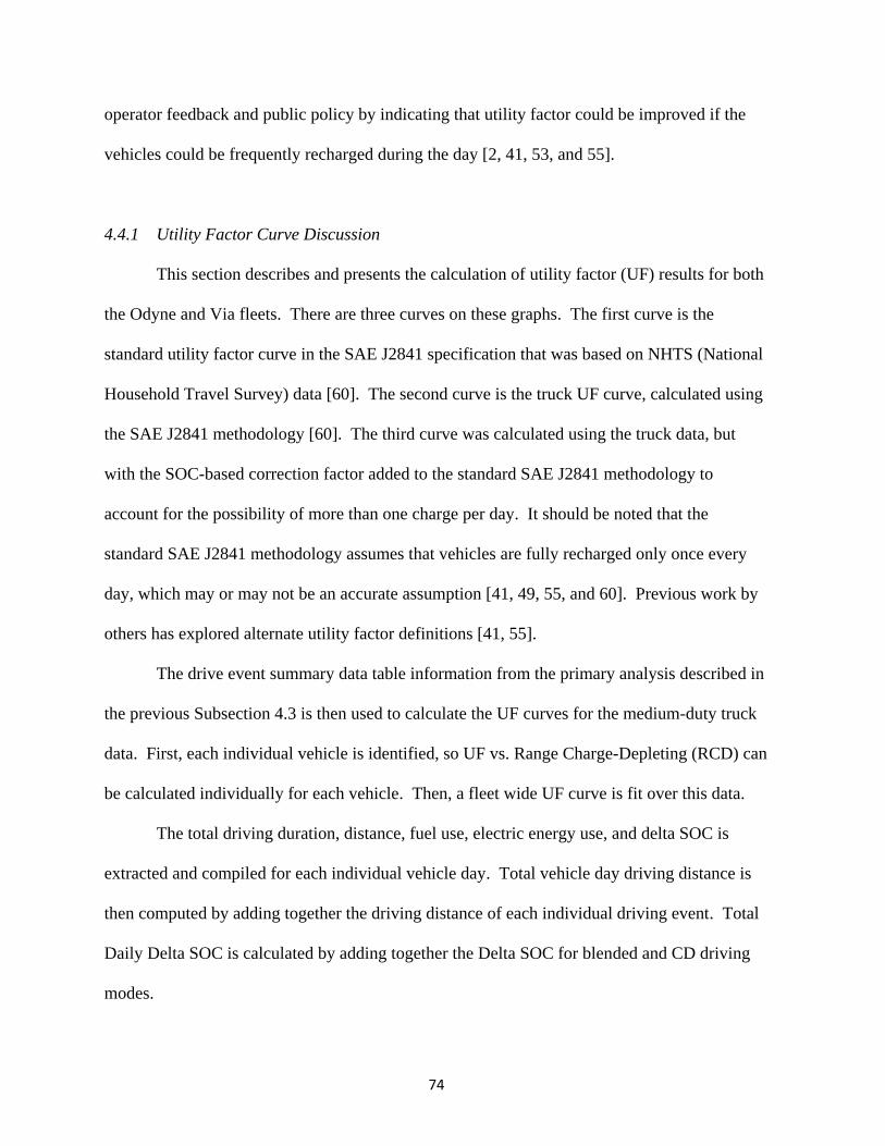
74

operator feedback and public policy by indicating that utility factor could be improved if the

vehicles could be frequently recharged during the day [2, 41, 53, and 55].

4.4.1 Utility Factor Curve Discussion

This section describes and presents the calculation of utility factor (UF) results for both

the Odyne and Via fleets. There are three curves on these graphs. The first curve is the

standard utility factor curve in the SAE J2841 specification that was based on NHTS (National

Household Travel Survey) data [60]. The second curve is the truck UF curve, calculated using

the SAE J2841 methodology [60]. The third curve was calculated using the truck data, but

with the SOC-based correction factor added to the standard SAE J2841 methodology to

account for the possibility of more than one charge per day. It should be noted that the

standard SAE J2841 methodology assumes that vehicles are fully recharged only once every

day, which may or may not be an accurate assumption [41, 49, 55, and 60]. Previous work by

others has explored alternate utility factor definitions [41, 55].

The drive event summary data table information from the primary analysis described in

the previous Subsection 4.3 is then used to calculate the UF curves for the medium-duty truck

data. First, each individual vehicle is identified, so UF vs. Range Charge-Depleting (RCD) can

be calculated individually for each vehicle. Then, a fleet wide UF curve is fit over this data.

The total driving duration, distance, fuel use, electric energy use, and delta SOC is

extracted and compiled for each individual vehicle day. Total vehicle day driving distance is

then computed by adding together the driving distance of each individual driving event. Total

Daily Delta SOC is calculated by adding together the Delta SOC for blended and CD driving

modes.

75

To build the utility factor curve, a vector of theoretical Range Charge-Depleting (RCD)

values is constructed from 0 to 300 miles, in increments of 0.5 miles. This and vehicle daily

total driving distance are then used to calculate a utility factor curve for each individual

vehicle. The following equation specified in SAE J2841 for the Fleet Utility Factor (FUF) [60]

is used for this calculation:

UF R = ∑ i dk,Rdk∈S∑ dkdk∈S (1)

In this equation, the Utility Factor (UF) is a function of the theoretical charge-depleting

range (RCD). dk is the daily driving distance of a single vehicle and S is the set of all daily

vehicle driving distance data.

Known sources of potential error in the standard SAE J2841 Fleet Utility Factor

calculation shown above are the assumptions that it is based on [55]. According to the SAE

J2841 Specification [60], there are two main assumptions that go into this calculation:

1) The vehicle starts the day from a routinely achieved, fully charged state.

2) The vehicle is charged to said state before every day of vehicle travel.

Based on these assumptions, the vehicle is only charged once per day. However, in the

real world, many PHEV vehicles are recharged multiple times, especially if there is a charging

station available at work or if the vehicle returns home multiple times throughout the day.

These multiple charges increase the effective utility factor of the vehicle.

An attempt was made to account for multiple charges per day by using the SOC signal

to calculate a modified SOC based utility factor. The below equations are used to calculate the

modified SOC based utility factor curve. These equations are a slight modification to the

standard SAE J2841 Fleet Utility Factor (FUF) equation:

76

�� � = ∑ i ��, ∙ ���∈� ∑ ����∈� (2)

�� = ax |∆ � �|, − � ���− � ��� (3)

In the SOC-based utility factor curve equation, Ck is a factor that increases the effective

RCD in the SAE J2841 Fleet Utility Factor equation, based on the total daily change in battery

State of Charge, ΔSOCk. To calculate ΔSOCk, the changes in state of charge values for every

vehicle trip in a day are added together. Note that the absolute value of ΔSOCk is taken to

ensure that the value is always positive. The term 100 - SOCCutoff represents the percent SOC

change that would occur during one fully charge-depleting trip. The SOCCutoff value represents

the battery state of charge level in which the vehicle transitions from a charge-depleting to a

charge-sustaining mode, and in this analysis the value was set to 5% for Odyne and 22% for

Via (as mentioned previously in Subsection 4.3.3) [15]. Note that the SOCCutoff value depends

on the specific model of vehicle and its hybrid control system architecture. The idea behind

the Ck factor is that if a vehicle recharges during the day in between trips, its ΔSOCk will be

greater than its 100 - SOCCutoff, thus increasing the true charge-depleting range of the vehicle

for the day. If ΔSOCk is less than 100 - SOCCutoff, the utility factor equation for the day will be

the same as the SAE J2841 utility factor. It should also be noted that if the vehicles are not

charged at least once per day, the SOC-corrected utility factor equation will output the exact

same curve as the standard SAE J2841 methodology.

Below in Figures 4.4 and 4.5 are the two graphs that summarize the utility factor curves

for both the Odyne and Via fleets:

77

Figure 4.4 - Odyne Utility Factor Curves

Figure 4.5 - Via Utility Factor Curves

78

For the medium-duty Odyne trucks, it can be seen that the UF is higher than the

standard SAE J2841 UF curve. From a design perspective, this means that these trucks can be

designed with a smaller battery than otherwise would be needed if the standard SAE J2841 UF

curve was used to meet performance requirements. From a policy perspective, medium-duty

trucks may not need as strict of emissions requirements as other commuter vehicles, as they are

inherently driven in such a way that increases UF. The SAE J2841 UF curve is just an average

of all vehicles in the US, whereas smaller subfleets within the set of all vehicles may have

different usage and UF curves [41, 49]. However, it should also be noted that Odyne trucks do

not operate in a true all-EV (electric vehicle) mode until the battery is depleted, which is an

assumption of the SAE J2841 methodology [15, 60]. Instead, the Odyne Trucks use a blended

CD vehicle mode where some gasoline power is used to extend the range of the electric

battery. So in reality, the actual gasoline displacement of the Odyne trucks will be less than the

gasoline displacement estimated by these UF curves. The actual gasoline displacement of

these vehicles could likely be improved if their control strategy was reprogrammed to have a

true-EV mode, or a blended-driving mode that used more electric power than the current

driving mode.

For the light-duty Via trucks, it can be seen that the UF is much closer to the standard

SAE J2841 UF curve than it is for the Odyne trucks. In this situation, it looks like the SAE

J2841 UF curve does a good job of approximating the actual real-world UF of Via trucks.

However, there is still a slight difference, so depending on the accuracy needed; the UF curve

presented in this paper may still be required. Unlike Odyne, the Via trucks operate in a true-

EV mode until the battery is nearly depleted, so the Via UF curves are likely representative of

their actual utility grid utilization in the field.

79

In the Odyne and Via truck UF curves, it is also interesting to see that the SOC

correction factor did not make a significant difference in the UF curve, so in this situation the

standard SAE J2841 assumption of only one charge per day appears to be very reasonable. It

is possible that the vehicles are only being charged once per day in line with the SAE J2841

standards, and if the charging pattern of the fleet changed, there could be a significant

difference between the two UF methodologies. To better understand the story of why these

two curves are so similar, charging event statistics are discussed next in Subsection 4.4.2 to

verify this hypothesis.

Overall, the truck UF curves show that light- and medium-duty commercial PHEV’s

are a great application for PHEV’s. The fact that their utility factor curves are equivalent to or

higher than the standard SAE J2841 curve means that on average, light- and medium-duty

truck PHEV’s can displace at least as much if not more gasoline than privately owned

commuter PHEV’s. Displacing gasoline with electric power can create many positive

economic and environmental benefits [2].

4.4.2 Charging Summary Statistics Discussion

Some additional charging event summary statistics were generated to better understand

the truck UF curves presented in the previous Subsection 4.4.1. Table 4.1 below presents these

numbers for both Odyne and Via:

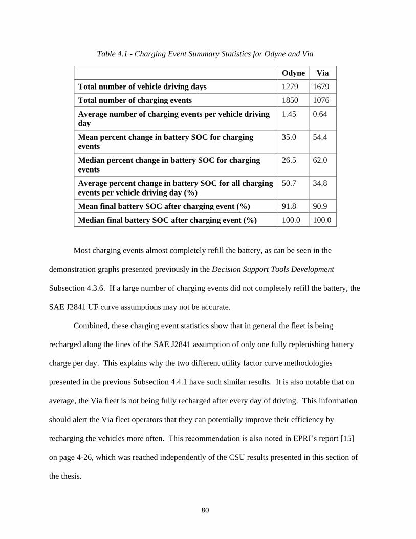
80

Table 4.1 - Charging Event Summary Statistics for Odyne and Via

Odyne Via

Total number of vehicle driving days 1279 1679

Total number of charging events 1850 1076

Average number of charging events per vehicle driving day

1.45 0.64

Mean percent change in battery SOC for charging events

35.0 54.4

Median percent change in battery SOC for charging events

26.5 62.0

Average percent change in battery SOC for all charging events per vehicle driving day (%)

50.7 34.8

Mean final battery SOC after charging event (%) 91.8 90.9

Median final battery SOC after charging event (%) 100.0 100.0

Most charging events almost completely refill the battery, as can be seen in the

demonstration graphs presented previously in the Decision Support Tools Development

Subsection 4.3.6. If a large number of charging events did not completely refill the battery, the

SAE J2841 UF curve assumptions may not be accurate.

Combined, these charging event statistics show that in general the fleet is being

recharged along the lines of the SAE J2841 assumption of only one fully replenishing battery

charge per day. This explains why the two different utility factor curve methodologies

presented in the previous Subsection 4.4.1 have such similar results. It is also notable that on

average, the Via fleet is not being fully recharged after every day of driving. This information

should alert the Via fleet operators that they can potentially improve their efficiency by

recharging the vehicles more often. This recommendation is also noted in EPRI’s report [15]

on page 4-26, which was reached independently of the CSU results presented in this section of

the thesis.

81

The Odyne fleet is charged more than once per vehicle driving day, but analysis

showed that a large number of charges only replenishing the battery by a very small amount

(see the previously presented graphs in the Decision Support Tools Development Subsection

4.3.6). Therefore, it is reasonable to conclude that the Odyne vehicles are being plugged in on

days when they are not driving and are already mostly charged.

From an operational perspective, there could be a lot of room for utility factor

improvement for both the Odyne and Via fleets if multiple charges could be facilitated

throughout the day [2, 15, 41, 53, and 55].1

4.5 Conclusions for Event Summary Data

The event summary methodologies presented in this chapter may be beneficial to future

vehicle tracking projects that require the analysis of high sampling frequency data from on-

board tracking sensors. The ability to summarize a large database of second-by-second driving

data points into a list of longer-term events is a particularly difficult task, especially when the

data collection devices are not 100% reliable. However, when compiled correctly, this event

summary list is also very useful. To demonstrate the utility of these event summary statistics,

utility factor curves, charging summary statistics, and demonstration histograms were

presented.

This work is also novel because it is the first time that UF curves have been published

for a fleet of medium-duty PHEV trucks. The presented UF charts for Odyne provide

1 All of the charging statistics presented in this section were calculated from the summarized event data using

about 80 lines of MATLAB code (including whitespace and comments) which ran on a single core in a matter of

seconds. The same analysis could have also been performed in Microsoft Excel. For comparison, the MATLAB

code written to create the event summary from the raw second-by-second driving CSV data was thousands of

lines of code, and took multiple days to run on a single core. Maintaining summarized event data can greatly

simplify, streamline, and expedite the data analysis process when new questions of research, design, operation,

or policy are posed.

82

additional evidence that different policies may be needed to govern different vehicle classes

and that a single overarching UF curve for every situation may not be appropriate [41].

The truck UF curves also show that light- and medium-duty trucks are an effective

application for PHEV technology, as light and medium-duty PHEV’s displace a large amount

of gasoline with electric power. These PHEV’s can displace at least as much gasoline as

privately owned commuter PHEV’s, if not more.

83

SECTION 5

CALCULATING VEHICLE EFFICIENCY AND CORRELATING IT TO OTHER

SIGNALS – METHODS AND RESULTS

5.1 Summary of Work

The work presented in this section originated from a class group project in my CS435

Big Data class where I learned how to use Java, Hadoop, and MapReduce to perform big data

analysis. The goal of this work was to use the EPRI Odyne and Via truck data described

previously to correlate vehicle efficiency to other signals and metrics. Some of the MATLAB

code that was used in this section (specifically Subsection 5.2) was similar to the code

developed for earlier work. The data management framework was improved from the original

framework described in Section 2 by myself and Mike Reid. Mike did the majority of the

restructuring.

The algorithm to analyze the data in this section was broken up into three consecutive

phases and code was developed independently for each phase. Each phase outputs a new

dataset that is the input data for the next data processing phase. The below flowchart in Figure

5.1 summarizes all of the high-level software phases that were created to perform the data

analysis presented in this chapter. Then, additional description for each step is provided below

the chart.

84

Figure 5.1 - High-Level Summary of the Fuel Economy Correlation Software

Phase 1 of 3 involves cleaning and filtering the raw data, identifying charge-depleting

drive events based on the algorithm explained in Section 4, and then splitting each charge-

depleting drive event into approximately 90-second drive intervals. The drive intervals are

approximate, because it is impossible to always divide any given length of driving time into

perfect 90-second intervals. Therefore, each drive event is divided into the number of

segments that would make the length of each division as close to 90 seconds as possible. The

raw second-by-second data for each of these 90-second drive segments is then written into a

CSV file with data from only that drive segment. These CSV files are used as the input to

Phase 2 of 3 which was written in Java for the Hadoop MapReduce framework. The idea is

that the fuel economy and other metrics can be calculated for each 90-second drive segment to

Download EPRI Data

Phase 0 / Data Extraction Function - Parse CSV files, validate data format, and write into .mat MATLAB data files. (from section 2)

Phase 1 - Identify Drive

Events and split into approximately 90-second segments. Uses MATLAB.

Phase 2 - Reduce each

90-second segment into a single data point

containing fuel economy and other statistics of

interest. Uses MapReduce.

Phase 3 - Calculate

Regression Model and Final Statistics of

Interest. Uses R for primary version.

Final Results

85

reduce each of these segments into a single data point. This discretizes the continuous data in a

way such that a regression model can be calculated. It was also important to break up the raw

data files into smaller chunks to avoid heap space errors in the Phase 2 MapReduce framework,

which uses a whole file input format.

The Phase 1 of 3 script is written in MATLAB and is similar to previous data

processing scripts. Phase 1 of 3 reads in the raw data from .mat files produced by the Data

Extraction Function described in Section 2. A slightly modified version of the Data Extraction

Function described in Section 2 was also created for a new data format provided by EPRI and

it was informally called Phase 0 of 3 since it came before Phase 1. However, the basic

principle and design behind this new Phase 0 is fundamentally the same besides compatibility

for the new data format. Phase 0 simply parses raw CSV files, verifies the CSV file format,

and writes out the data into .mat files. It should also be noted that parallel processing was not

implemented in the Phase 1 MATLAB code so it takes about a full day to process any of the

available datasets on a single core. More details about exactly how Phase 1 is implemented are

provided in Subsection 5.2.

Phase 2 of 3 is a MapReduce function written in Java. This MapReduce function was

run on a Linux computer cluster in the Computer Science department here at CSU. The goal of

Phase 2 is to read in each of the CSV files created by Phase 1 that represent about 90-seconds

of drive data and reduce each file into a single line of data. The Phase 2 output contains

information about the fuel economy, ambient temperature, kinetic intensity, whether the AC

was on, etc. Only a mapper in the MapReduce framework is needed to perform this reduction.

Since this code can run in parallel and is scalable to large computer clusters, this analysis only

86

takes about an hour to run on a Hadoop computer cluster with 15-20 machines. More details

about exactly how Phase 2 is implemented are provided in Subsection 5.3.

Phase 3 of 3 is where the regression model, visualizations, and any final filtering steps

are implemented. The input to Phase 3 is a single CSV file produced from the output to Phase

2. Graphs and regressions can then be created based on the raw data. A few different Phase 3

implementations were created. The first Phase 3 implementation uses MATLAB to plot the

vehicle efficiency against other variables, such as ambient temperature, kinetic intensity, cabin

temperature, etc. The second Phase 3 implementation is written in MapReduce and performs a

linear-regression model with k-fold validation. The advantage of the MapReduce

implementation is that it is scalable to much larger datasets, but the disadvantage is that much

of the regression calculation has to be programmed from scratch using linear algebra so the

regression model could be calculated in pieces running on parallel computers. The third

implementation of Phase 3 was written in R and this is likely the best implementation of Phase

3. The R implementation is similar to the MATLAB implementation, except that R provides

better statistical tools to calculate confidence intervals on the regression line and other statistics

of interest. Other function shapes besides a linear model were also experimented with in R and

these produced slightly better results. More details about exactly how Phase 3 is implemented

are provided in Subsection 5.4 and sample results are provided in Subsection 5.5.

I would like to thank Joseph Minicucci and Mike Reid for helping me write the

software to implement the algorithms that I developed to perform this analysis. A large

amount of software development was required to produce these results and I would not have

had time to do everything myself. This was a very large project and it would not have been

possible without a group effort.

87

5.2 Details of Phase 1 Analysis Implementation – Data Cleaning, Filtering, and

Splitting

This subsection is divided into two additional lower-level subsections. The first

subsection (5.2.1) details the data filtering and processing algorithm that was implemented in

the Phase 1 analysis software. The second subsection (5.2.2) presents and reviews some of the

data validation tools that were developed to provide more information about the impact of each

data processing step in the Phase 1 implementation.

5.2.1 Details of the Phase 1 Analysis Algorithm

The Phase 1 script was written in MATLAB and can operate on four different datasets.

Both the Odyne and Via platforms have an old dataset and a new dataset. However, only the

old Odyne dataset is used for most of the results presented later in Subsections 5.5 and 5.6. A

small portion of the presented results used the new Via dataset as well.

Like the Analyze_all_data function described in Subsection 2.3, controlling variables

are defined at the beginning of the script. The user also has the option to toggle diagnostic

plots on and off. If the data is organized in subdirectories, the user has the option to define the

subdirectory folder names. It was a lot easier to just hard code the subdirectory names for this

application than program MATLAB to search through all of the file folders.

The script will loop through each individual .mat data file and process each of the files

separately. These .mat data files are created from the raw CSV files using the Phase 0 / Data

Extraction Script which is not discussed here. See Subsection 2.2 for more information about

the data parsing and extraction process used to create the .mat files. If the raw data file does

not have at least 1000 data points when all of the different signals are counted together, the file

88

will be skipped. Each raw data file should contain data from one vehicle for one month, or if

the data size for one vehicle month is too large then the Phase 0 / Data Extraction Script could

have produced multiple .mat data files for one vehicle month. Then, each raw CAN-

communication bus signal is parsed from the raw data format so that the data points from each

signal can be saved into a separate vector. The script produces an error if there were no data

points for a signal name.

In the new data formats for Odyne and Via which are not extensively used in the

presented analysis results, each raw signal needs to be sorted by timestamp to ensure that all of

the data points are in a sequential order. In the new data, most timestamps are ordered

sequentially in local groupings, but these local groupings are also not arranged sequentially.

This might be a result of the Hadoop system used by EPRI’s contractor to manage the raw

data, as Hadoop software has a tendency to write output data in a random order. Fortunately,

in the old datasets used for most of this analysis, the raw data was already pre-sorted.

After each individual CAN signal is sorted, another filter removes data points with

values outside of a realistic range of values for that signal. This is also referred to as “Filter 1”

in the next Subsection 5.2.2 and Table 5.1 where the impact of each data filter is quantified.

The exact values of the realistic range are just determined by using basic engineering

judgement and common sense. There is no formula used to derive these values. For example,

an ambient temperature of 100 degrees Celsius does not make sense in the real world as we

know that the atmosphere is not at boiling temperature. Below are the acceptable value ranges

that were chosen to filter each signal in the dataset. Data points outside of these ranges are

deleted.

89

Ambient Temperature: [-30, 50] deg C

Battery Voltage: [0, 600] Volts

Battery Current: [-400, 400] Amps

Battery State of Charge (SOC): [0, 100] Percent

Vehicle Speed: [0, 200] kph

Odometer: [0, 500000] miles

Cabin Temperature: [-30, 50] deg C

After the range of each signal is checked, the next step is to count the number of data

points in each signal in the data file. If any of the above signals have less than 100 data points

in a data file, the data file will be skipped. This is also referred to as “Filter 2” in the next

Subsection 5.2.2 and Table 5.1.

Next the data is run through a filter to remove duplicate timestamps. This is also

referred to as “Filter 3” in the next Subsection 5.2.2 and Table 5.1. There is an uncommon

glitch in the data where a sensor will report two different values for the same timestamp and

this causes execution problems later in the software if the duplicate timestamps are not

removed.

Again, the length of every signal in the data file is checked after the duplicate time

stamp filter to see if the filter reduced the data size below the required threshold of 100 data

points per signal. In this case, no additional data files were removed, but it is good to check

one final time after any filter that removes data because it is always possible that a data file

will be made too short. This is also referred to as “Filter 4” in the next Subsection 5.2.2 and

Table 5.1.

90

After duplicate timestamps are removed, all of the CAN signals are then interpolated

onto the speed timestamp values. The vehicle speed timestamps were chosen to be the

projection target because these data points are generally recorded when the vehicle is driving.

This aligns the asynchronous data collection from multiple sensors onto the same set of

timestamps so different signals can be compared directly using the same timestamp values.

This is very similar to the process used and described previously in Subsection 4.3.3.

Then, the drive event identification algorithm previously explained in Section 4 is used

to identify where charge-depleting drive events occurred with some adjustments to the

algorithm parameters. Here are the parameters that were used to tune the performance of the

algorithm from Subsection 4.3.3 for this situation:

Minimum Speed to Identify Drive Event = 0.01 kph

Minimum SOC for Charge-Depleting mode = 6 % (Odyne)

Minimum Allowable Drive Event Duration = 90 secs

Minimum Allowable Time Gap Between Drive Events = 30 secs

Minimum Number of Data Points Allowed in an Event = 20

In addition, to simplify the analysis, charge-depleting and charge-sustaining modes are

not redefined based on additional available information for each drive event such as the change

in SOC and the fuel injection rate, as explained in Subsection 4.3.3. This is a difference

between the analysis methodologies presented in Subsection 4.3.3. In this analysis, the

blended driving mode of the Odyne trucks is considered to be a charge-depleting mode and is

referred to as such in this section.

91

Once each charge-depleting drive event is identified, the algorithm splits up each drive

events into approximately 90-second drive segments that can later be reduced into single data

points in a regression model. The goal is to discretize continuous data. For this discussion, a

drive event is defined as the data from when the vehicle started driving to when it stopped

driving (while ignoring short, brief stops by the vehicle). A drive segment is defined as an

approximately 90-second interval of data within a drive event.

The length of each drive segment varies depending on the length of each drive event as

it is normally not possible to divide a drive event up into perfect 90-second intervals. It was

decided that it is better to have slightly uneven drive segment times than drive segments with

large amounts of non-driving time beyond the end of the drive event. Including a large amount

of non-driving time in a drive segment would essentially amount to a very short drive segment

and give unequal weighting to that short time period at the end of the drive event in the

regression model.

To check that the data interpolation is working properly across the drive segments and

events, the software counts the number of pre-interpolation data points for each CAN signal

after “Filter 4” that are contained within the drive interval. This is to see if the interpolated

estimations for each CAN signal are based on nearby data points of actual recorded data for

that signal. This is one improvement over the analysis methodology presented in Subsection

4.3.3. If a drive event or segment does not contain any actual pre-interpolation data points, the

interpolation over that drive event or segment is not going to be accurate.

Any drive event that does not have at least one actual data point for ambient

temperature, AC switch state (on/ off), heater switch state (on/off), or cabin temperature is

ignored and output for that event is suppressed. These are referred to as the “long-term

92

signals.” Any drive segment within a drive event that does not have at least 20 data points for

engine fuel injection rate, battery voltage, battery current, and battery state of charge is ignored

and output for that event is suppressed. These are referred to as the “short-term signals.”

These two categories of checking the entire drive event vs. the drive segment are based on how

quickly the signal values generally change and are recorded by the data collection system.

Signals such as the ambient temperature and whether the heater is on or off tend to be longer-

term signals that are generally more stable over longer periods of time, so their values can be

more safely extrapolated across the larger time range of an entire drive event. The other

signals change more rapidly and must have data points recorded in each individual drive

segment. Note that not all versions of the data and vehicle models record all of these signals,

so if a platform does not have all of the mentioned signals in the raw data, the software only

checks for the signals that are available and the final data analysis is adjusted accordingly.

If a drive segment of approximately 90 seconds of length has all of the required drive

signals during the data interpolation check, the different signals are compiled and written out

into a unique CSV file that only contains data from that drive segment. In this CSV file each

CAN-communication signal is placed into a separate column and the timestamp values are

used as the row labels. Each CSV file should have approximately 90 rows of data. A unique

key that can be used as a key in the MapReduce Framework is also generated for each drive

segment. The key contains unique identifying information for each drive segment in a text

string so the individual drive segments can be kept separate if needed.

This completes the description of the Phase 1 data processing algorithm. After the CSV

files are written out by this process, they need to be uploaded onto a Hadoop Cluster (which

uses the HDFS file system) so they can be processed by the Phase 2 MapReduce function.

93

Section 5.2.2 provides a description of some of the data validation tools that were built into the

MATLAB Phase 1 software and provides an initial quantitative assessment of the impact from

the data filtering steps described in this section.

5.2.2 Review of the Validation Tools That Were Built Into the Phase 1 Process and What

They Reveal About Data Filtering

During the MATLAB Phase 1 process, a number of validation tools were built into the

software to verify that each data processing and filtering step was working correctly. The goal

was to produce some diagnostic output for the intermediate data processing steps to better

understand how those steps were impacting the real-world data in practice. This helped

prevent the software from becoming a “black-box” algorithm where only input and output data

would be accessible and the inner workings of the software would be obscured.

For example, a number of graphs can be generated for each data file to visually verify

that the process is working correctly. A graph of speed vs. time for each drive event is

produced and vertical-red lines indicate where the drive event is being split into the

approximately 90-second drive segments. An example of one of these graphs is shown in

Figure 5.2. Note that the timestamps on the x-axis are in a MATLAB serial date format. This

tool was very helpful to debug the software and it helped identify problems in the first versions

of the software where the start and end timestamps for each drive event did not line up with the

actual data.

By looking through the collection of these graphs it is easy to visually identify where

drive segments are not being appropriately identified or divided. Since there are a large

number of data files, it was not practical to have a human examine every single graph.

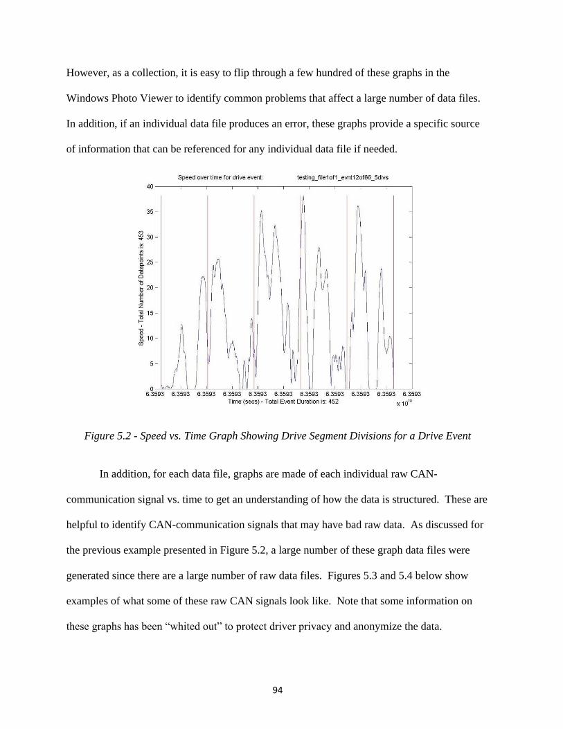
94

However, as a collection, it is easy to flip through a few hundred of these graphs in the

Windows Photo Viewer to identify common problems that affect a large number of data files.

In addition, if an individual data file produces an error, these graphs provide a specific source

of information that can be referenced for any individual data file if needed.

Figure 5.2 - Speed vs. Time Graph Showing Drive Segment Divisions for a Drive Event

In addition, for each data file, graphs are made of each individual raw CAN-

communication signal vs. time to get an understanding of how the data is structured. These are

helpful to identify CAN-communication signals that may have bad raw data. As discussed for

the previous example presented in Figure 5.2, a large number of these graph data files were

generated since there are a large number of raw data files. Figures 5.3 and 5.4 below show

examples of what some of these raw CAN signals look like. Note that some information on

these graphs has been “whited out” to protect driver privacy and anonymize the data.

95

Figure 5.3 – Battery SOC Signal (in %) vs. Time

Figure 5.4 - Current from the Main Vehicle Battery (Amps) vs. Time

96

A number of additional graphs that plot multiple signals on top of each other are also

produced by the software to see how the different sensor signals align before the data

interpolation step. These graphs help to better understand how the data is being interpolated

during the data interpolation step. See Figures 5.5 and 5.6 below for examples of these graphs.

The point of this diagnostic tool is to overlay all of the signals that are needed to analyze drive

events when vehicle speed data points are being recorded. It can be seen that most of the raw

signals that are used in the drive event data analysis are only recorded when the vehicle speed

is greater than zero. In this graph, the red points are vehicle speed, the green points are AC

switch state, the cyan points are ambient temperature, the magenta points are cabin

temperature, and the dark blue data points are heater switch states. Note that some of the

signals have been multiplied by a constant so the different signals all scale to a similar size

when they are superimposed onto the same graph. The purpose of these graphs is not to see the

true quantitative values of the signals. It is to see when the data points are being recorded

relative to the other signals.

97

Figure 5.5 - Thermal Systems Signals

Figure 5.6 - Thermal Systems Signals (Zoomed in)

Color Key:

Vehi le Speed

AC Swit h State O =

A ie t Te perature

Ca i Te perature

Heater Swit h States O =5

Color Key:

Vehi le Speed

AC Swit h State O =

A ie t Te perature

Ca i Te perature

Heater Swit h States O =5

98

Finally, in addition to the visual graphs that are generated by the software to aid in the

debugging process, the data analysis script contains counter variables to track how many data

points, data files, drive events, and approximately 90-second drive segments remained after the

different data-filtration steps. This provides information about the actual impact these data

filtering steps have when applied to the real-world vehicle data. The final counter values after

all of the Odyne data was processed are presented in the following three tables (Tables 5.1, 5.2,

and 5.3) and one figure (Figure 5.7).

Table 5.1 shows the number of data points remaining for each individual CAN signal

before those data points are projected onto the same time stamp values in the data interpolation

step. Note that data is asynchronous and each unique CAN signal has a different number of

data points. Table 5.2 shows the number of raw data files that were loaded initially and the

number of data files that had enough signals to actually be used for the analysis. Table 5.3

summarizes the data filtering steps after all of the CAN signals are interpolated onto the same

set of timestamp values.

99

Table 5.1 – Number of Data Points Remaining After Each Individual Data Filtering Step

Before the Time Stamp Interpolation

CAN Signals

used in Analysis

RAW - Number of Data

points for each

specific signal in all

raw data files before

any data filtering

FILTER 1 - Number of data

points after Filter 1,

which checks that

each data point falls

within an acceptable

range for the signal

and remove outliers

FILTER 2 - Number of data

points after Filter 2,

which removes any

data files where any

CAN signal in that file

has less than the

required number of

data points after

Filter 1

FILTER 3 - Number of data

points after Filter 3,

which removes

Duplicate Time

Stamps

FILTER 4 - Number of data

points after Filter 4,

which removes any

data files where any

CAN signal in that

file has less than the

required number of

data points after

Filter 1

AC 19120068 N/A 11682104 11519643 11519643

Heat 19118643 N/A 11681989 11519512 11519512

Fuel Injection Rate 35236325 35236325 26823526 26349674 26349674

Ambient

Temperature7143466 7142968 4436786 4368418 4368418

Battery Voltage 216268335 216268335 133843107 131597486 131597486

Battery Current 216268374 216228533 133843020 131597423 131597423

Odometer 10213277 10211332 8770931 8585474 8585474

SOC 80218917 80218917 52429475 51117262 51117262

Speed 5525692 5525692 5383072 5247686 5247686

Cabin

Temperature7143466 7130675 4428884 4360654 4360654

Total Data Points

from All Signals616256563 616201488 393322894 386263232 386263232

Data Filtration Steps

Direction of Data Processing Flow

100

Table 5.2 – Data File Filtering Summary

Table 5.3 – Data Filtering Steps After the Linear Interpolation Step

Data File Filtering Summary

Total data files loaded initially753

Total data files fully processed and written out - No processing

errors such as too few data points397

Data Filtering Steps after all CAN signals are

interpolated onto the same set of time stamps

(listed in sequence of processing order)

Total number of unique time stamps after interpolation (same

as the vehicle speed data point count after Filter 4) 5247686

Total number of Charge Depleating events identified

14391

Total number of Charge Sustaining events identified

2227

Total number of unique time stamps in all identified CD drive

events 3864768

Total number of Charge Depleating events that had sufficient

pre-interpolation data points between the start and end

timestamps for what are defined as "long-term" signals

13708

Total number of approximately 90-second drive segments

calculated from all remaining CD events after the previous

long-term pre-interpolation data point check

41951

Drive Segment Filter 1 - Total number of approximately 90-

second drive segments that contained enough short-term pre-

interpolation data points for all short-term signals

39157

Drive Segment Filter 2 - Total number of approximately 90-

second drive segments that contained the minimum number of

interpolated data points

39157

101

In addition, the results in Table 5.1 were plotted into a bar chart using MS Excel for

easier visualization. See Figure 5.7 below:

Figure 5.7 – Results Plotted from Table 5.1: Data Points Remaining After Pre-Interpolation

Data Filtration Steps

Notable details related to the data presented here in Tables 5.1 - 5.3 and Figure 5.7 are

listed below:

In Table 5.1, the total raw data point count does not include small data files that

were initially ignored because they contained less than the minimum required

102

number of data points, which was 1000 data points for all signals combined. Since

these files only have a few data points, leaving them out of the raw data point count

at the beginning should not significantly decrease the number of raw data points

recorded in the first column of Table 5.1.

In Table 5.1, note that the AC and Heat signal data point counts under Filter 1 are

listed as “N/A.” This is because the range filter does not apply to AC and Heat

signals since they are discrete on/off values instead of continuous data. For the total

number of data points in Table 5.1 and Figure 5.7, the raw AC and Heat data point

count is also used as the count after Filter 1.

In Table 5.2, the total number of data files loaded initially does include the small

data files that are immediately ignored because they contained less than the

minimum required number of data points, which was 1000 data points from all

signals combined.

Not all of the numbers presented in Table 5.3 are counts of individual data points.

This table also includes some statistics about the number of drive events and the

drive segments that each event is split into.

In Table 5.3, the number of charge-sustaining events is only included for reference.

Charge-sustaining events are not used in the data analysis process.

See Section 5.2.1 for more details about each specific step in the data-filtration

process and the sequence of data processing and filtering steps.

103

After reviewing the results of the data-filtration step counters presented above, here are some

notable observations:

1) When referencing Figure 5.7, it is surprising that so few vehicle speed data points

were collected. This is important because all of the other signals are interpolated

onto these timestamps. It is possible that the data collection system could be

improved by collecting more of these data points to improve the interpolation

accuracy. Unfortunately, it is unlikely that any other CAN signal timestamps could

have been used for the interpolation target in this situation. It might be possible to

use the fuel injection rate on Odyne, but since these vehicles also have an electric

motor that can be used for propulsion, it is possible that in some situations the fuel

injector would not be used when the vehicle is driving. The Odometer signal is

known to have some faulty data on Via so this might not be the best signal to use

for the interpolation projection target either. Some of the electrical signals such as

SOC, battery current, and battery voltage are recorded for other truck operation

modes in addition to driving, such as Odyne’s stationary and charging mode, so

these would not be a good choice for the interpolation target either.

2) The raw number of data points removed by each filtration step should not be the

only consideration when determining that filter’s effectiveness. For example,

although Filter 3 in Table 5.1 only removed a small number of data points, the data

interpolation step later in the process would have crashed if the software did not

filter these duplicate timestamps.

3) Filter 2 removed the largest number of data points when it is compared to the other

data-filtration steps. This filter removes entire data files that do not contain the

104

minimum number of data points for each signal, which in this case is 100 data

points. This means that a large number of data files are missing at least one of the

required signals listed in Table 5.1 and there could be an opportunity to improve the

reliability of the data collection system on Odyne Vehicles. It is unknown why so

many signals were missing from the original dataset.

4) Filter 4 in Table 5.1 did not remove any data points. This is because the previous

duplicate time stamp filter only removed a small amount of data and no individual

CAN signal in any individual data file dropped below the minimum number of

required data points after Filter 3. However, it is still a good idea to include Filter 4

in the overall process when analyzing other datasets because it is possible that a few

files may still need to be removed when the algorithm is used in other applications.

5) In Table 5.3, it can be seen that checking if each drive event or segment contains

enough pre-interpolation data points for each individual signal removes a

significant number of drive events and segments. About 5% of the drive events

were removed because they did not contain enough long-term signal data points

such as the AC on/off CAN signal. Then, once the remaining drive events were

split into drive segments, about 7% of those segments were removed because they

did not contain enough short-term signal data points such as the battery current

CAN signal. It is possible that the removed percentage of data is large enough to

have a significant impact on the final results, depending on the level of accuracy

desired in the calculation.

105

5.3 Details of the Phase 2 Analysis Implementation – Reducing Drive Segments Into

Single Data Points

For this portion of the analysis the Hadoop MapReduce framework is used and

MapReduce functions are written in Java [29, 33]. Hadoop is a Distributed File System (DFS)

that runs on a Linux computer cluster and it is commonly known as the Hadoop Distributed

File System (HDFS). MapReduce is a data analysis framework that runs on top of Hadoop to

efficiently process large amounts of data in parallel. To use MapReduce, one generally writes

a mapper function that parses the data files, a reducer function that combines the output of the

mapper function, and a main driver function that controls the job parameters and overall

execution. Data is organized into key / value pairs where the key is used to group the data and

the value represents the actual data values. For this analysis only a mapper function was used

and the input was set to a whole file input format that would read in the entire CSV file for

each drive segment into a single mapper. The MATLAB code in Phase 1 was used to pre-split

the data to avoid heap space errors that can be encountered when using a whole file input

format in the mappers.

The algorithm for the Phase 2 process is much simpler than for the Phase 1 process. In

Phase 2, a mapper in the MapReduce framework is used to reduce each of the CSV data files

that are output from the Phase 1 process into a single data point. The mapper function first

parses each CSV file to identify the individual signals. Then, trapezoidal integration is used to

calculate fuel consumption, electricity consumption, and total distance traveled using the fuel

injection rate, speed, battery voltage, and battery current signals. Battery power is calculated

by multiplying the voltage and current signals from the battery and then integrating. Other

values, such as ambient temperature, AC on / off (0 or 1 values), and the battery state of charge

106

are just averaged over the 90-second drive segment to produce a single data point for that drive

segment. Kinetic intensity is also calculated during this step to give another value to which the

efficiency data could be correlated [46]. Kinetic intensity can be used to measure driver

aggressiveness. The goal is to provide a number of different predictor variables that can be

correlated against the response vehicle-efficiency variable.

An equivalent vehicle efficiency is then calculated using the electric and fuel

efficiency. This is done by using the energy equivalency of diesel fuel. The conversions used

are 1 gallon of gasoline = 33.44 kWh [61, 62] and 1 gallon of diesel has 113% the energy

density of 1 gallon of gasoline by volume [63].

All of this data is output by the mapper function into individual files that each

contained a single line of data. These are then combined into a single CSV file that contains all

of the fleet data using Hadoop’s getmerge command. Alternatively, a basic reducer function

can also be switched on in the main driver class of the MapReduce code to combine the

mapper output into any number of data files. It should be noted that MapReduce writes output

in a random order so there is no defined sequence in the order of the output data. Once this

single CSV file is created for all of the fleet data, it can be analyzed using the Phase 3 code to

produce regression results and other statistics of interest.

I would like to give special thanks to Joseph Minicucci for implementing the Phase 2

algorithm into Java code for MapReduce. He did a great job of organizing the code and

creating a clean script to execute this algorithm effectively. The results presented later would

not have been possible without his implementation.

107

5.4 Details of the Phase 3 Analysis Implementation – Regression Models

Once the data reaches the Phase 3 analysis software, it is no longer a “big data”

problem due to the data reduction and summarization steps in Phases 1 and 2. However, all of

the data still resides in a CSV file with about 30,000 lines of data and a process is still needed

to interpret this data. Three different frameworks were created to do this. Alternatively, it

would also have been possible to analyze the Phase 2 output data using Microsoft Excel,

although that option was not pursued for this project.

The first Phase 3 framework is written using MATLAB. It plots all of the data points

and creates a number of linear-regression models to check how vehicle efficiency might

correlate against other variables. On the Odyne trucks the equivalent fuel economy is

compared against ambient temperature, AC switch states, cabin temperature, heater switch

states, kinetic intensity, and vehicle calibration. The electric only fuel economy is also

compared to ambient temperature. Vehicle calibration is a control state that is programmed

into only the Odyne trucks and it is either mild or aggressive. A mild calibration slows down

the rate of battery depletion and uses more gasoline during the charge-depleting mode to

extend the battery range, while an aggressive calibration does the opposite [15]. Discrete

values, such as vehicle calibration, AC on/off, and heater on/off are represented by zero or one

values so a regression can be drawn. Drive segments where the switch state transitions from

off to on are represented as fractional values that represent the proportion of time that the

switch state was on or off. In addition, a few other statistics such as the average fuel economy

for both mild and aggressive calibrations are calculated. Finally, extreme outliers are filtered

out from the input data for this script before the regression models are calculated. The

108

description of the Phase 3 R framework later in this subsection has more information about this

outlier filtering process.

The second Phase 3 framework was developed for the CS435 Big Data analysis class at

CSU and it uses MapReduce to calculate a linear-regression model piecewise. The least

squares equation from linear algebra is used in a way that allows regression models to be

calculated on subsets of the data. The regression models for the subsets can then be added

together in the reducer phase to produce the entire regression model. This framework also

performs k-fold testing. For scientific work, this framework is not used to publish results, as

the data is not large enough to justify parallel computations and the other single core methods

are much simpler, easier to debug, and troubleshoot. K-fold validation is also not used in the

presented scientific results in this document.

The third framework developed for the Phase 3 analysis component is similar to the

MATLAB framework except that it was developed using the R programming language. In

addition, the R framework implements a final data filtering step before the regression was run.

For the ambient temperature signal, any Odyne data points outside the range of -10 to 49

degrees C are removed from the regression model. In addition, any equivalent fuel economy

data points outside the range of -10 to 50 miles per gallon are removed from the regression

model. These outliers are considered beyond the expected realistic range of values for this

data. It is not clear why the Phase 1 and 2 software produced these outlier data points, but it is

believed that they can be safely removed from the regression model as they only represent

about 1% of the data in the old Odyne dataset and do not fall within a realistic range of values.

Before this final filtering step on the Odyne dataset, R had 39,153 data points loaded from the

Phase 2 CSV output file. After this filtering, 38,761 data points remained. These filters were

109

then applied to the MATLAB script described previously that can be run as an alternative to

the R script. Finally, additional models besides a linear model are fitted to the data, such as a

semi-log and quadratic model, to see if a better fit could be achieved.

5.5 Sample Results from the Vehicle Efficiency Correlations

Results from the Phase 3 R script are presented using the old Odyne dataset. There is a

new dataset for both Odyne and Via that contains data collected from a wider range of dates,

but only a little of the analysis on the new Via dataset is presented in Subsection 5.5.6 and it

did not produce meaningful results. The new dataset is required to correlate ambient

temperature to vehicle efficiency for Via as the ambient temperature signal is not present in the

old Via dataset. Hopefully, future work can present higher quality results based on this new

data. The old Odyne dataset was the same dataset that was used for the results in Section 4 so

refer to that section for more details about the data used for this analysis.

5.5.1 Vehicle Efficiency vs. Ambient Temperature – Linear and Quadratic Models for Odyne

First, all of the data points from the approximately 90-second drive intervals are plotted

on a graph of equivalent fuel economy (mi/gal) vs. ambient temperature (deg C). Both linear

and quadratic models are fit to this data. The quadratic model tests if the data has the same

trend at both low- and high-ambient temperatures, but results show that the quadratic function

is very close to the linear function with a slight curve. The scatterplot with these regressions is

presented in Figure 5.8 below:

110

Figure 5.8 - Trend in Equivalent Fuel Economy vs. Ambient Temperature for Odyne Trucks

On the linear model, the p-values for the regression coefficients are less than 2x10-16

where the null hypothesis is that the true coefficient is equal to zero. On the quadratic model

the p-values are higher but still very small. The R-squared values are also small. The linear

model has an R-squared of 0.005780 and the quadratic model has an R-squared of 0.006234.

Since the p-values on the regression model are small and the R-squared values are low, it can

be concluded that the models are poor predictors for any individual data point, but they also do

represent the overall average trend seen in the global collection data points. Therefore, this

model could be used as an average to represent the overall fleet performance at these different

111

temperatures, but it could not be used to predict the fuel economy of any individual driver for

any individual trip or 90-second drive interval. Below (in Figure 5.9, Figure 5.10, Table 5.4,

and Table 5.5) is the console output from R with these results, as well as a table that

summarizes key parameters from the console output:

> summary(Fit)

Call:

lm(formula = 1/equivalentFuelEconGalPerMile ~ avgAmbientTempInC,

data = filteredData)

Residuals:

Min 1Q Median 3Q Max

-6.925 -2.249 -0.653 1.467 43.013

Coefficients:

Estimate Std. Error t value Pr(>|t|)

(Intercept) 6.10060 0.04582 133.13 <2e-16 ***

avgAmbientTempInC 0.02702 0.00180 15.01 <2e-16 ***

---

Signif. codes: 0 ‘***’ 0.001 ‘**’ 0.01 ‘*’ 0.05 ‘.’ 0.1 ‘ ’ 1

Residual standard error: 3.541 on 38751 degrees of freedom

Multiple R-squared: 0.00578, Adjusted R-squared: 0.005755

F-statistic: 225.3 on 1 and 38751 DF, p-value: < 2.2e-16

Figure 5.9 - R Code Console Output for the Linear Regression Model

Table 5.4 - Coefficients and Values for the Linear-Regression Model of Vehicle Efficiency vs.

Ambient Temperature

Parameter Estimated value p-value y-intercept 6.10060 (mi/gal) Less than 2x10-16 slope 0.02702 (mi/(gal*C)) Less than 2x10-16 R-squared 0.00578 N/A

112

> summary(Fit2)

Call:

lm(formula = 1/equivalentFuelEconGalPerMile ~ poly(avgAmbientTempInC,

2, raw = TRUE), data = filteredData)

Residuals:

Min 1Q Median 3Q Max

-6.837 -2.252 -0.651 1.469 42.961

Coefficients:

Estimate Std. Error t value Pr(>|t|)

(Intercept) 5.8764362 0.0702665 83.631 <2e-16 ***

poly(avgAmbientTempInC, 2, raw = TRUE)1 0.0539407 0.0066461 8.116 4.95e-16 ***

poly(avgAmbientTempInC, 2, raw = TRUE)2 -0.0006267 0.0001489 -4.208 2.59e-05 ***

---

Signif. codes: 0 ‘***’ 0.001 ‘**’ 0.01 ‘*’ 0.05 ‘.’ 0.1 ‘ ’ 1

Residual standard error: 3.54 on 38750 degrees of freedom

Multiple R-squared: 0.006234, Adjusted R-squared: 0.006183

F-statistic: 121.6 on 2 and 38750 DF, p-value: < 2.2e-16

Figure 5.10 - R Code Console Output for the Quadratic Regression Model

Table 5.5 - Coefficients and Values for the Quadratic-Regression Model of Vehicle Efficiency

vs. Ambient Temperature

Parameter Estimated value p-value a - intercept 5.8764362 (mi/gal) Less than 2x10-16 b – linear term 0.0539407 (mi/(gal*C)) 4.95x10-16 c – quadratic term -0.0006267 (mi/(gal*C2)) 2.59x10-5 R-squared 0.006234 N/A

Equation is of the form: y = a + bx + cx2 = equivalent fuel economy

Next, a residual and QQ-plot were constructed for the linear model explained above.

This is shown below in Figure 5.11. It shows that the data is skewed and not normally

distributed.

113

Figure 5.11 - Residual and QQ-Plot for the Linear Model of Ambient Temperature vs.

Equivalent Fuel Economy

5.5.2 Vehicle Efficiency vs. Ambient Temperature – Semi-Log Model for Odyne

To correct the problem of skewed and non-normally distributed data in the previous

Subsection 5.5.1, the data was replotted on a semi-log scale based on a natural logarithm and

the linear-regression model was redrawn. The graphs and table below (Figures 5.12 – 5.14,

and Table 5.6) show the new regression, residual plot, and QQ-plot. These graphs show that

the semi-log transformation improves the assumptions behind the linear model, but it is still not

perfect. The trend of lower fuel economy at higher temperatures remains in the semi-log

regression model. It is unclear what kind of regression model would create a near-perfect QQ-

plot.

114

Figure 5.12 – Semi-Log Regression of Equivalent the Fuel Economy vs. Ambient Temperature

Figure 5.13 – Residual and Normal QQ-Plot for the Semi-Log Regression Model of Ambient

Temperature vs. Equivalent Fuel Economy

115

> summary(Fit3)

Call:

lm(formula = log(1/equivalentFuelEconGalPerMile) ~ avgAmbientTempInC, data = filteredData)

Residuals:

Min 1Q Median 3Q Max

-3.5584 -0.2876 0.0177 0.3175 2.1402

Coefficients:

Estimate Std. Error t value Pr(>|t|)

(Intercept) 1.7035909 0.0064891 262.53 <2e-16 ***

avgAmbientTempInC 0.0035091 0.0002549 13.77 <2e-16 ***

---

Signif. codes: 0 ‘***’ 0.001 ‘**’ 0.01 ‘*’ 0.05 ‘.’ 0.1 ‘ ’ 1

Residual standard error: 0.5015 on 38751 degrees of freedom

Multiple R-squared: 0.004866, Adjusted R-squared: 0.00484

F-statistic: 189.5 on 1 and 38751 DF, p-value: < 2.2e-16

Figure 5.14 - R Code Console Output for the Semi-Log Regression Model

Table 5.6 - Coefficients and Values for the Semi-Log Regression Model of Vehicle Efficiency

vs. Ambient Temperature

Parameter Estimated value p-value y-intercept (a) 1.7035909 ( ln(mi/gal) ) Less than 2x10-16 Slope (b) 0.0035091 ( ln(mi/gal)/C ) Less than 2x10-16 R-squared 0.004866 N/A

Model is: ln(y) = a + bx = ln( equivalent fuel economy )

The trends seen in these graphs for vehicle efficiency follow the same pattern as the

trends for conventional gasoline vehicles established in the 1980’s [64]. In this EPA sponsored

report titled Temperature Correction Formulas for Adjusting Estimates of Automobile Fuel

Consumption [64] it can be seen on page 8 that fuel consumption is higher at lower

temperatures, which corresponds to the lower fuel economy in miles per gallon seen in the

Odyne fuel economy regression lines that were calculated by CSU. This makes sense, as the

Odyne truck is still mostly a gasoline powered vehicle with mild-electric hybridization [15].

116

Therefore, the general qualitative ambient temperature trends from conventional gasoline

vehicles can still be applied to mild hybrid PHEV vehicles such as Odyne Medium Duty Work

Trucks. The similarities between the CSU model and this EPA model are further explored

later in Subsection 5.6.1.

5.5.3 Vehicle Efficiency vs. Kinetic Intensity for Odyne

In addition to the ambient temperature results, vehicle efficiency was also regressed

against other variables to look for other correlations. The most significant trend was found in

the kinetic intensity [46]. Kinetic intensity (KI) can be used as a measure of driver

aggressiveness with higher kinetic intensity values corresponding to more aggressive driving

behavior. As would be expected, vehicle efficiency decreases as driver aggressiveness

increases. The R plot below (Figure 5.15) shows this trend.

117

Figure 5.15 - Vehicle Equivalent Efficiency vs. Kinetic Intensity

The regression model for ambient temperature vs. kinetic intensity has the following

parameters and R-console output (Figure 5.16 and Table 5.7):

118

> summary(Fit4)

Call:

lm(formula = 1/equivalentFuelEconGalPerMile ~ kinematicIntensityOneOverKm,

data = filteredData)

Residuals:

Min 1Q Median 3Q Max

-5.568 -2.003 -0.590 1.258 42.127

Coefficients:

Estimate Std. Error t value Pr(>|t|)

(Intercept) 6.1539 0.0171 359.85 <2e-16 ***

kinematicIntensityOneOverKm -1.1784 0.0375 -31.42 <2e-16 ***

---

Signif. codes:

0 ‘***’ 0.001 ‘**’ 0.01 ‘*’ 0.05 ‘.’ 0.1 ‘ ’ 1

Residual standard error: 3.157 on 38759 degrees of freedom

Multiple R-squared: 0.02484, Adjusted R-squared: 0.02482

F-statistic: 987.3 on 1 and 38759 DF, p-value: < 2.2e-16

Figure 5.16 - R Code Console Output for the Linear-Regression Model of Fuel Economy vs.

Kinetic Intensity

Table 5.7 - Coefficients and Values for the Linear-Regression Model of Kinetic Intensity vs.

Ambient Temperature

Parameter Estimated value p-value y-intercept 6.1539 (mi/gal) Less than 2.2x10-16 slope -1.1784 (mi*km/gal) Less than 2.2x10-16 R-squared 0.02482 N/A

The residual and QQ-plot for the equivalent fuel economy vs. kinetic intensity model

are shown below in Figure 5.17. Like the previous linear model for ambient temperature vs.

equivalent fuel economy, although the linear model is not the best model for the data, it does

highlight that the basic trend is that fuel efficiency decreases as kinetic intensity increases.

This is the expected qualitative result.

119

Figure 5.17 - Residual and QQ-Plot for the Linear Model of Equivalent Fuel Economy vs.

Kinetic Intensity

5.5.4 Correlations between Vehicle Fuel Economy and Vehicle Drivetrain Calibration for

Odyne

Another factor that was investigated to understand its correlation to the Odyne vehicle

efficiency is the powertrain calibration. When an Odyne truck is programmed with a mild

calibration, the vehicle uses more gasoline during its charge-depleting mode to save battery

power. When the truck is programmed with an aggressive calibration, the vehicle uses less

gasoline and more battery power during its charge-depleting mode. Since all of the collected

data falls into these two discrete categories, a 2-sample-t-test is used to calculate the mean

value for each category and the p-value. Before the statistical test was run, it was expected that

the results would be statistically significant due to the very large sample size. The t-test is just

an extra measure to ensure the significance of the results.

120

The two sample t-test shows that the fuel economy for the mild and the aggressive

calibrations are very similar. The Welch-Satterthwaite method is used. The fuel economy

during the charge-depleting mode for a vehicle programmed with a mild calibration is 6.705

mpg. The fuel economy during the charge-depleting mode for a vehicle programmed with an

aggressive calibration is 6.791 mpg. These results are statistically significant as the p-value is

0.02345. However, since the calculated values are so similar, it is likely that this difference is

not the most significant factor that influences vehicle fuel economy in the real world and is of

debatable practical importance.

It should also be noted that filtering outliers has a large impact on all of the above

results. For example, if the unfiltered data is instead used for the vehicle calibration 2-sample

t-test, the mild calibration gets a fuel economy of 9.947 mpg and the aggressive calibration gets

a fuel economy of 6.745 mpg. However, the p-value of p = 0.2921 for these results is not

generally considered to be statistically significant.

A different result with a much larger p-value is also true for some of the other

regression models presented in earlier subsections before the filtering was implemented,

although the exact values for each regression model without this filtering are not presented in

this thesis. However, as removing outliers is generally considered to be an acceptable

statistical practice and the removed data points did not have realistic values, we believe that

these results still meet acceptable statistical practices [65]. This filtering process was

explained previously in more detail.

121

5.5.5 Correlations between Vehicle Efficiency and Other Variables for Odyne

In addition, some of the other signals are investigated for trends against the equivalent

fuel economy in the old Odyne dataset. These include the HVAC signals and the cabin

temperature signal.

Cabin temperature showed a similar correlation to vehicle efficiency as ambient

temperature, which makes sense as the temperature inside the vehicle is often similar to the

temperature outside the vehicle. The data from these results will not be directly presented in

this thesis, but it is worth mentioning that they were investigated as well.

It was discovered that the heater and AC signals are not turned on enough to calculate

any meaningful trend. It is theorized that AC and heater use might have an impact on vehicle

efficiency in cold and warm temperatures and there are other studies that support that AC use

impacts vehicle efficiency [42, 43].

5.5.6 Vehicle Efficiency vs. Ambient Temperature for Via

Of particular interest is the correlation between the electric fuel economy (in

miles/kWh) of Via’s pure-electric charge depleting mode and ambient temperature. Some

initial evidence from work published by Tugce Yuksel and Jeremy J. Michalek suggests that

the driving efficiency of pure electric vehicles has a different correlation to ambient

temperature than gasoline vehicles [56].

To investigate this correlation in our own dataset, we used the same algorithm for

Odyne with some minor code modifications to make it run on the new Via dataset. Unlike

most of the other analysis presented in this paper, the new Via dataset that was hosted on AWS

was used since that was the only way to access the ambient temperature signal. Unfortunately,

122

the final results from this analysis did not make sense. After the 90-second drive segments

with a battery SOC of less than 22% were removed, the majority of the 90-second drive

segments still had significant gasoline fuel usage reported by the algorithm. This contradicts

what we understand about the Via powertrain from EPRI’s report [15] and the Via Corporate

Website [21, 22] which both state that Via operates with a pure-EV charge depleting mode.

Below in Figure 5.18 is a histogram that shows the distribution of the gasoline-only fuel

economy in Via’s charge-depleting mode without the equivalent electric fuel use included into

the fuel economy calculation. It can be seen that a large number of the 90-second drive

segments show significant fuel consumption. If data points where the reported fuel economy is

greater than 0.001 gal/mile are removed from this dataset, the number of data points decreases

from 121984 to 23205 which is about an 80% reduction. CSU concluded that this filtration

step is removing too many data points for there to be confidence in final results so final results

will not be presented here.

123

Figure 5.18 – Problem With the Via Recorded Gasoline Consumption in Charge Depleting

Mode

It is unclear why so much fuel consumption is being reported for the Via platform when

it is supposed to be in a pure-EV charge depleting mode. It is possible that the algorithm does

not work when it is applied to other vehicle platforms or it is possible that our team could have

introduced a bug into the software when it was converted to run on the Via dataset. It is also

possible that there is a problem with the Via onboard data collection system or that we do not

fully understand how the Via hybrid powertrain is operating in the real world. Or, it is also

possible that some of the new Odyne data got mixed into the new Via data in the new database

storage system that was only used for the Via analysis presented here. Finally, the general

124

impression of the Odyne vs. the Via dataset was that Odyne contained more accurate and

complete data than Via so that could be part of the problem as well. All of these possibilities

might be contributing to the problem.

Since there is uncertainty in these results, the correlation between equivalent fuel

economy and ambient temperature for Via will not be presented. Hopefully future research can

resolve these issues as the results of a pure-EV electric efficiency vs. ambient temperature are

expected to be significant for the research community.

5.6 Discussion

5.6.1 Comparison of Odyne Fuel Economy vs. Ambient Temperature Trends to a

Conventional Vehicle

We can use the Odyne results to understand the effect that ambient temperature has on

the fuel economy of these vehicles. In this discussion section, we compare the fuel economy

sensitivity to ambient temperature correlation that is calculated in this study for Odyne to the

correlation calculated in another study.

First of all, in the 1980’s the EPA commissioned a study to understand the effects of

ambient temperature on conventional vehicle fuel economy [64] and the Odyne results

presented here follow the same trend. The EPA study shows that at cold temperatures, vehicles

in general use more fuel. At 0 degrees F in the EPA study, the gasoline engine uses

approximately 1.14 times more fuel than it does when it is operating in the standard FTP

temperature range of 68 deg F to 86 deg F [64]2. This difference disappears once the ambient

temperature reaches the lower bound of the FTP temperature range in the EPA study as the

2 Data from the EPA study was derived graphically by using logarithmic interpolation on the graph presented on

page 8 of this study. Results from the graphical interpolation are approximate.

125

number is a ratio to the FTP fuel consumption. This can be compared to our ambient

temperature results from the EPRI Odyne dataset by dividing the predicted miles per gallon

value from a point within the FTP temperature range ( in this case (68 + 86) / 2 = 77 deg F ) by

the predicted miles per gallon at 0 degrees F. At 0 degrees F our semi-log model from the

EPRI data predicts a fuel economy of 5.161 mpg. At 77 degrees F our semi-log model predicts

a fuel economy of 5.997 mpg. This calculation results in a cold temperature increase in fuel

consumption of 1.16 times when the cold-temperature fuel consumption is compared to the

fuel consumption in the middle of the FTP temperature range. Again, these results are based

on our real-world data model. As you can see, the fuel consumption increase of 1.16 times for

Odyne is reasonably similar to the fuel consumption increase of 1.14 calculated in the EPA

report for the same temperature [64].

Table 5.8 below shows a comparison of this ratio between our Odyne dataset and the

EPA data over a range of other temperatures:

Table 5.8 - Comparison of the Fuel Economy vs. Ambient Temperature Results

Temperature (deg F) 0 20 40 60 80 100

EPA FE Ratio – For Conventional Gasoline Engines

[64]

1.14 1.11 1.06 1.02 0.99 1.00

FE Ratio from our EPRI data (semi-log model) – for

mild-hybrid electric Odyne

trucks

1.16 1.12 1.07 1.03 0.99 0.96

126

It can be seen in Table 5.8 above that our Odyne dataset closely follows the EPA

dataset. The biggest divergence occurs at 100 deg F because the EPA study uses a different

semi-log model for temperatures about the FTP range whereas our study used a single semi-log

model for the entire data range.

Since the Odyne truck is a mild hybrid and still produces most of its torque and power

using a conventional diesel engine, it makes sense that the Odyne truck would follow the same

general trend as a conventional vehicle. The electric motor on the Odyne truck only provides a

small power assist to improve the fuel economy.

5.6.2 How Ambient Temperature Could Impact Fuel Economy at Temperature Extremes

According to EPRI the Odyne Trucks have a fuel economy rating of 6.07 mpg on the

CILCC drive cycle when they are programed with a mild-calibration setting that depletes the

battery more slowly [15]. Assuming that this drive cycle test was performed at room

temperature (23 deg C), our semi-log model from the EPRI Odyne data suggests that

temperature could influence the fuel economy results by increasing the equivalent fuel

economy by 6% when the temperature is increased to 40 deg C or lowering the equivalent fuel

economy by 11% when the temperature is reduced to -10 deg C. These differences could have

meaningful real-world impacts. These percentages are calculated from our semi-log model

where the fuel economy at 23 deg C is 5.955 mpg, the fuel economy at 40 deg C is 6.321 mpg,

and the fuel economy at -10 deg C is 5.304 mpg. Percentage results for Odyne are calculated

by dividing the extreme temperature fuel economy by the standard fuel economy at 23 deg C. .

127

5.6.3 The Potential Impact of HVAC on Fuel Economy

In addition, as discussed earlier in Subsection 5.5.5, the AC and heater were almost

never turned on according to the data analysis of the old Odyne dataset so our real-world data

is expected to be closer to the type of data in the EPA report that is based on drive cycle

testing. HVAC is generally not accounted for during an EPA drive cycle test. However, it is

known that AC can impact the fuel economy of a vehicle so if the heater and AC were used in

the Odyne Trucks these results could have been much different. In work published by Kiran

Kambly and Thomas H. Bradley [42, 43], the effects of ambient temperature and HVAC use

on vehicle efficiency were investigated. In Detroit Michigan, it was shown that the all-EV

range of PHEVs varied between 65 and 79 miles and this variation was due to differences in

ambient temperature conditions and HVAC use [43]. Therefore, if the HVAC systems of the

Odyne trucks were more widely used, this could impact the equivalent fuel economy vs.

ambient temperature curve by lowering the fuel economy at extreme cold and hot ambient

temperature conditions. Another dataset with more HVAC usage would be needed to

quantitatively determine the impact of HVAC on Odyne fuel economy and verify that it

changes the fuel economy in this situation. Or, it is also possible that there is a glitch in our

data analysis software and that is why we are seeing these results.

128

SECTION 6

DISCUSSION

6.1 Why the Methodologies behind Big Transportation Fleet Data Analysis Need to be

Better Defined

Many studies have presented the final results of fleet data analysis [1, 15, 43, 48, 49,

50, 51, 52, 53, 54, 55, 56, and 57] but few of these studies really provide a detailed description

of the analysis methodologies, assumptions, and intermediate data processing steps that were

used to draw their conclusions. Having done this type of fleet data analysis work myself at

Colorado State University, my experience has been that the final results can be dependent on

the assumptions, filtering techniques, data manipulations, and other intermediate steps that are

used to produce the results. More work is needed to understand the impact of these data

processing steps, how they affect the final results, and what data processing steps represent the

“best practice” for analyzing vehicle fleet-tracking big data.

6.1.1 The Impact of Outlier Filtering Just before the Regression Model is Calculated

For example, as previously discussed in Subsections 5.4 and 5.5.4, if outliers are not

filtered out in the intermediate data after the Phase 2 processing and just before the regression

model is drawn, different results that are not statistically significant are generated. If the

unfiltered data is instead used for the vehicle calibration 2-sample t-test, the mild calibration

gets a fuel economy of 9.947 mpg and the aggressive calibration gets a fuel economy of 6.745

mpg with a p-value of p = 0.2921. This is very different than the mild-calibration fuel

economy of 6.705 mpg, the aggressive-calibration fuel economy of 6.791 mpg, and the p-value

129

of p = 0.02345 that were calculated when outlier data filtering was applied. Table 6.1 below

summarizes these differences:

Table 6.1 - Comparison of Fuel Economy and P-Values With and Without Outlier Filtering

With Outlier Filtering

Without Outlier Filtering

Mild-Calibration Fuel Economy (mpg)

6.705 9.947

Aggressive-Calibration Fuel Economy (mpg)

6.791 6.745

p-value 0.02345 0.2921

6.1.2 The Impact of Continuously Evaluating the Drive Condition in the Data Analysis

Software

The above example about removing outliers is a common statistical practice that is

fairly well known. However, to process vehicle fleet-tracking data our team also had to

develop a number of more obscure methods that are very specific to this type of data analysis.

For example, another known problem with the raw data is the data collection system only

collects data when the vehicle is operating. Therefore, data collection may begin a few

seconds after the vehicle turns on and recorded values such as the vehicle speed and battery

current do not start at zero like you would expect in perfect theoretical data. The graph below

in Figure 6.1 shows an example from the raw Odyne data where the battery current signal does

not start at zero. You can see how MATLAB interpolates the battery current in a straight line

over a time span of about two days, because the first battery current data point collected was

approximately -40 Amps when the vehicle turned on again. However, since the vehicle only

130

uses battery power when the vehicle is on, the true battery current that occurs immediately

when the vehicle turns on should be very close to zero.

Figure 6.1 - Raw Battery Current Signal (Amps) Does Not Start at Zero as Seen in the

Interpolation Error

This is a very specific problem with vehicle tracking data. The next question is, what

problems can this cause and how do we deal with it? In our process described in Section 4, the

analysis code does not look for trigger events when a threshold is crossed, such as when the

vehicle speed transitions from a near zero to positive value, to identify when the vehicle starts

and stops driving. Instead, the analysis code defines a continuous condition that is applied to

all of the data points to check if the vehicle speed is greater than zero. This way, if the data

collection system misses the initial few seconds when vehicle speed transitions from 0 mph to

positive, the driving event identification algorithm can still figure out that the vehicle is driving

131

even if the first driving speed data point is at, let’s say, 30 mph. This is a very subtle

difference in the analysis methodology, but it can have real impacts on the results.

For example, the data in Figure 6.2 below shows drive event summary data that was

compiled by a different, preliminary algorithm while it was still under development at another

EPRI contractor (independent of CSU). This algorithm had problems properly identifying

where charging events should occur as can be seen in the below results. In Figure 6.2 below

that shows the event summary data, there should be a charging event between the highlighted

driving events, especially when the second drive event begins with the battery mysteriously

recharged. After conversations with EPRI’s software contractor, CSU realized that one of the

reasons behind these problems was that their algorithm only checked if the signal was

transitioning across a threshold and did not consider if the initial value was already beyond the

threshold.

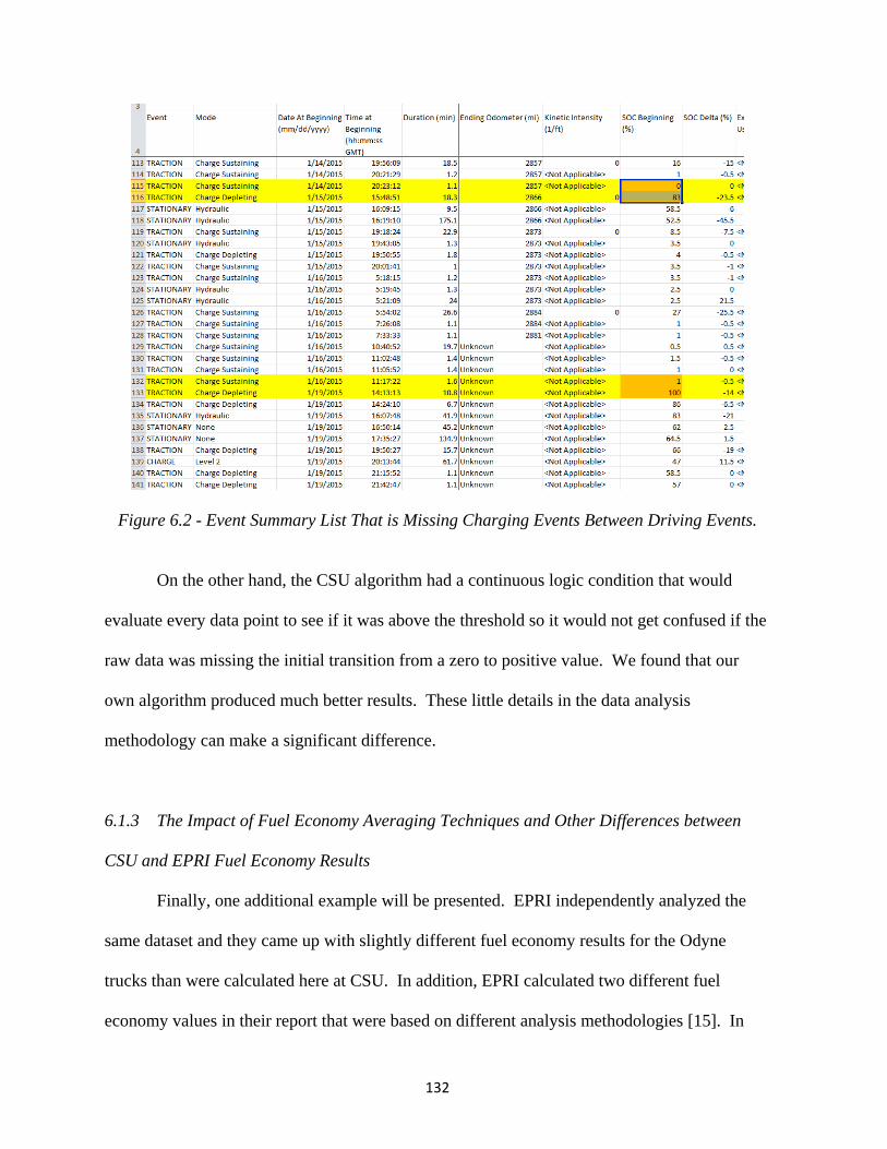
132

Figure 6.2 - Event Summary List That is Missing Charging Events Between Driving Events.

On the other hand, the CSU algorithm had a continuous logic condition that would

evaluate every data point to see if it was above the threshold so it would not get confused if the

raw data was missing the initial transition from a zero to positive value. We found that our

own algorithm produced much better results. These little details in the data analysis

methodology can make a significant difference.

6.1.3 The Impact of Fuel Economy Averaging Techniques and Other Differences between

CSU and EPRI Fuel Economy Results

Finally, one additional example will be presented. EPRI independently analyzed the

same dataset and they came up with slightly different fuel economy results for the Odyne

trucks than were calculated here at CSU. In addition, EPRI calculated two different fuel

economy values in their report that were based on different analysis methodologies [15]. In

133

EPRI’s report on their Figure 3-28 [15] (NOT Figure 3-28 in this thesis), they list the mild-

calibration fuel economy as 5.8 (± 1.5) mpg and the aggressive-calibration fuel economy as 6.1

(± 1.6) mpg for Odyne. However in the EPRI report on their Figure 3-41, they list the mild-

calibration fuel economy as 6.19 mpg and the aggressive-calibration fuel economy as 6.65

mpg. In addition, for comparison, CSU calculated the mild-calibration equivalent fuel

economy to be 6.71 mpg and the aggressive-calibration equivalent fuel economy to be 6.79

mpg based on the data analysis process described in Section 5 of this thesis.

If everyone is using the same data to calculate these results, why are all of these

numbers different? One difference between the EPRI and CSU analysis is that CSU is

reporting an equivalent fuel economy that factors the electricity usage into the fuel economy

whereas EPRI is reporting the diesel only fuel economy. However, if the EPRI fuel and

electric fuel economies from their Figure 3-28 [15] are combined into an equivalent fuel

economy, we still see a difference between the EPRI and CSU fuel economy values.

By using data from EPRI’s Figure 3-28 in their report [15], the mild-calibration

equivalent fuel economy was calculated to be 5.58 mpg and the aggressive-calibration

equivalent fuel economy was calculated to be 5.53 mpg. This calculation was performed by

combining the diesel only fuel economy with the average drive energy / distance data that is

provided in the same table. The same formula that was used for the CSU equivalent fuel

economy calculation in the Phase 2 MATLAB process described in Subsection 5.3 was applied

to the EPRI data. Note that fuel economy decreases when electric energy is accounted for, as

more energy use is being reported. Our equivalent fuel economy calculations could have

possibly been improved by accounting for fuel vs. electric efficiency ratios as well, but this

was not implemented into our software.

134

Table 6.2 below compares these different fuel economy numbers for all of the different

situations described above. It should be noted that all of the different reported fuel economy

values fall within EPRI’s reported tolerance range for the data reported in Figure 3-28 in their

report [15] so this is a positive indication that the different results provide a reasonable

approximation of the true fleet fuel economy.

Table 6.2 - Comparison of Different Odyne Fuel Economies Calculated Using the Odyne Real-

world Data

CSU Analysis Results

EPRI Analysis

Results from their Figure 3-41 (diesel

only fuel economy) [15]

EPRI Analysis

results from their Figure 3-28 (diesel

only fuel economy) [15]

Calculated equivalent

fuel economy from EPRI results in

their Figure 3-28 [15]

Mild-Calibration Fuel Economy (mpg)

6.71 6.19 5.8 ± 1.5 5.58

Aggressive-Calibration Fuel Economy (mpg)

6.79 6.65 6.1 ± 1.6 5.53

Another difference between the different methodologies developed by EPRI and CSU

is how the data is being averaged. In EPRI’s Figure 3-28 in their report [15], the average fuel

economy is calculated by dividing the total number of miles driven by the fleet by the total

amount of gasoline used by the fleet. However, in EPRI’s Figure 3-41 in their report [15], they

are averaging the daily average fuel economies presented as a distribution in their histogram.

Although neither of these two methods is necessarily “right” or “wrong”, they are also not

mathematically equivalent and should be considered different statistical measures. For another

comparison, the CSU fuel economy calculation used neither of the two EPRI methods

135

described above. At CSU, we averaged the average fuel economies over 90-second drive

intervals, which is different than averaging the average-daily fuel economies. This raises some

questions. How should average fuel economies be reported for this type of work and do these

differences matter? It will be left to future researchers to answer this question.

There are other differences between the EPRI and CSU data analysis processes as well

since they were developed independently. For example, EPRI calculated drive events by using

the key on/off signal to identify where a drive event was occurring whereas CSU checked if the

vehicle speed signal was greater than zero. Or, CSU only used data from charge depleting

(CD) drive events whereas EPRI used all drive data. In addition, EPRI may have a wider range

of data as CSU only used a subset of the total dataset. There could be other unknown

methodology differences between the EPRI and CSU results as well.

Overall, all of these methodology differences could be contributing to the difference in

the final results. Depending on the accuracy needed, it will be left up to the reader and future

researchers to determine if the differences between these fuel economy numbers is practically

significant enough to pose a risk to their application or reported fuel economy results. The

good thing is that all of the presented numbers are reasonably close to each other so they could

each be used as a valid estimator of the unknown real-world fuel economy.

6.1.4 Conclusion: Why More Data Analysis Methods Need to be Better Defined

A few examples of why methodologies need to be defined for analyzing vehicle fleet-

tracking data were presented with evidence. As can be seen in Sections 4 and 5, there are

many other data processing steps that could influence the final results which are not discussed

in this discussion section. A flaw in any of these steps could produce inaccurate scientific

136

results that would mislead policy makers, fleet owners, and vehicle designers. My research

team believes that there needs to be a published “cookbook” of methodologies for analyzing

vehicle fleet-tracking data and we hope that the work presented in this thesis can lay an initial

foundation to begin a discussion about how these best practices should be defined. There is

plenty of room for future researchers to build on the work in this thesis by evaluating the

effectiveness and impact of each individual data processing step and by developing new data

analysis techniques.

6.2 Advantages of Making Decisions Based on Real-World Fleet Data

This section outlines some of the potential benefits of using real-world fleet data to

make operational and policy decisions. Real-world data can provide an alternate evaluation

method to EPA drive cycles and it can also be used to calculate the real-world utility factor.

6.2.1 Real-World Data Provides an Alternate Evaluation Method to EPA Drive Cycles

Historically, the standard method to evaluate vehicle emissions and fuel economy was

testing the vehicle on an EPA drive cycle [66]. These drive cycles define exactly what speed

the vehicle should be driving at over time and are typically 700 to 1000 seconds long. The

tests are normally performed on a dyno setup, which is a highly controlled environment. This

provides great experimental repeatability for different vehicle platforms to be tested against.

However, there are also disadvantages to using EPA drive cycles.

One disadvantage of EPA drive cycles is the assumption that a 10-minute test can

accurately represent real-world driving behavior. Other studies have investigated this and

many have found that drive cycles often produce different results than those produced using

137

real-world data [11, 52, 67, and 68]. In theory, results calculated from real-world data should

accurately represent how the vehicles performed in the real world so real-world data has the

potential to provide more accurate information about vehicle use, emissions, and fuel economy

to policy makers. It is debatable if a 1000-second drive cycle can fully capture all of the

intricacies of driving behavior and vehicle use such as the weather conditions experienced,

differences in driving behavior between individual drivers, local traffic laws, variations in

traffic conditions, and changes in vehicle performance due to aging. However, collecting real-

world data accounts for all of the factors that can possibly affect vehicle performance whether

those factors are known or unknown. Below is some sample data from our own work to

demonstrate this.

For example, according to EPRI the Odyne Trucks have a fuel economy rating of 6.07

mpg [15] on the CILCC drive cycle [69] when they are programed with a mild-calibration

setting that depletes the battery more slowly [15]. Odyne trucks programmed with an

aggressive-calibration setting have a fuel economy rating of 7.72 mpg on the same drive cycle

[15]. On drive cycle tests, the aggressive calibration gets better fuel economy than the mild

calibration. However, in our final data calculation from the code described in Section 5, CSU

found that the fuel economy was very similar for the mild and aggressive calibrations. The

average equivalent fuel economy for a mild calibration was 6.71 mpg and the average

equivalent fuel economy for an aggressive calibration was 6.79 mpg based on the data analysis

work performed at CSU on the real-world Odyne truck dataset. This illustrates that the fuel

economy can be different when it is calculated using an EPA drive cycle vs. using real-world

data.

138

In addition, different EPA drive cycles produce different fuel economy results. On the

OCTA drive cycle the Odyne trucks get an average fuel economy of 4.44 mpg for a mild

calibration and an average fuel economy of 5.57 mpg for an aggressive calibration [15]. Or, on

the HHDDT drive cycle [69] the Odyne Trucks get an average fuel economy of 5.46 mpg for a

mild calibration and an average fuel economy of 7.09 mpg for an aggressive calibration [15].

The differences between the different EPA drive cycle results raises the question of which EPA

drive cycle most accurately represents real-world driving. The fuel economy from all of these

EPA drive cycle tests and our real-world results are summarized below in Figure 6.3. As can

be seen, there are differences between our real-world fuel economy calculations and the fuel

economy calculations from the different EPA drive cycles.

Figure 6.3 - Real World vs. EPA Drive Cycle Fuel Economy Comparison [15]

Finally, real-world data collection is important because EPA drive cycles are

susceptible to cheating, such as in a recent incident involving Volkswagen that was heavily

139

publicized in the news [70, 71]. In this scandal, Volkswagen programmed their vehicles to run

the engine differently to reduce emissions when its control system recognized an EPA drive

cycle pattern. These discrepancies were first noticed when researchers started measuring the

emissions of vehicles driving in the real world. Therefore, real-world data such as the EPRI

data used in this study can be used to verify that OEM’s are not programming their vehicles to

cheat EPA drive cycle tests. When large-scale real-world data collection is implemented,

OEM’s who build vehicles have to make their vehicles emit appropriate emissions because it is

very difficult to cheat the real world.

6.2.2 Real-World Data Can be Used to Calculate Real-World Utility Factors

A utility factor, such as the utility factor (UF) curves presented in Section 4.4.1 and

presented in previous work [1, 41, 49, 55, and 60], is needed to calculate the environmental

impact of a range-extending vehicle such as a PHEV. Utility factor is a proportion that tells

what proportion of driving distance is being powered in a charge-depleting drive mode where

electric energy from the utility grid is used. For example, a utility factor of 80% means that

80% of the driving distance occurs in a charge-depleting mode that is using power from the

electric utility grid. If the PHEV has an all-EV charge depleting mode, the utility factor

represents the actual proportion of the driving distance that was only powered by the electric

utility grid.

Utility factor is frequently presented as a graph of UF vs. the charge-depleting range of

the battery (RCD) so vehicle designers can make trade-off decisions about what battery size is

needed in the vehicle. A large onboard battery will increase the UF as the vehicle will then be

able to make longer trips on a single charge. However, there are also diminishing returns in

140

UF improvement as the battery size continues to increase as there are generally fewer and

fewer people making longer and longer trips. Utility factor is also highly dependent on driving

behavior, as drivers who mostly take very short trips and recharge in between will have a much

higher UF than drivers who take their PHEV vehicles on long-distance trips across the country.

The SAE J2841 standard is commonly used to define UF [60], but different vehicle

platforms and real-world effects can influence the UF to be different in specific situations [41].

Real-world driving data is needed to determine how a specific subset of vehicles might differ

from the SAE J2841 standard UF curve. In addition, the SAE J2841 standard UF curve was

based on NHTS data which is self-reported by drivers in the study [47] so vehicle sensor data

such as the data used in our study may provide more accurate results and eliminate human

error.

For example, the following figure (repeated from Subsection 4.4.1 and relabeled Figure

6.4) shows how the Odyne UF curve that was calculated from our dataset differs from the

standard SAE J2841 UF curve.

141

Figure 6.4 - Odyne Utility Factor Curves

In addition, the Via UF graph (repeated from Subsection 4.4.1 and relabeled as Figure

6.5) shows that there is a smaller difference from the standard UF curve than is seen in the

Odyne UF graph. However, there is still a difference. For a Via battery with 25 miles of

range, the standard SAE2841 curve indicates that the vehicle would power approximately 56%

of its driving using power from the electricity grid. However, the UF curve calculated using

real-world data indicates that the Via vehicle would power approximately 52% of its driving

using power from the electricity grid using the same sized battery. This difference could still

be large enough to make a real-world impact depending on the required accuracy.

142

Figure 6.5 - Via Utility Factor Curves

6.3 How Valid Are These Final Data Analysis Results?

After considering the presented information and the discussion so far, considering if the

results are valid is a fair question to ask. The short answer to this question is: maybe, but more

work is needed to better define and understand the data processing methodologies for vehicle

fleet tracking data.

6.3.1 Reasons Why Our Final Results Might Be Valid

In addition to the discussion presented previously in Subsection 6.2 about the benefits

of using real-world fleet tracking datasets, one could argue that since our results for the

ambient temperature vs. vehicle efficiency calculation are so similar to the previous EPA study

for conventional vehicles, this is a positive indication that the results could be reasonably

accurate. Odyne did not produce any outrageous results that were totally unrealistic so this is

143

also a good indication that supports the validity of our results. For example, our real-world

average fuel economy (presented previously in Figure 6.3) falls within the range of the

different EPA drive cycle tests so it may be a valid estimator of real-world fuel economy.

Since our fuel economy results are close to the EPA drive cycle results and the

independent EPRI analysis on the same dataset, this provides additional evidence that our

analysis method is providing a reasonable approximation for the average fuel economy. These

results were discussed previously in Subsection 6.1.3.

Finally, because the Via is likely driven in a similar manner to other light-duty vehicles,

it seems reasonable that its utility factor curve (presented earlier in Figure 6.5) is close to the

J2841 standard utility factor curve. As documented in this thesis, a large number of data

filtering, quality control steps, and intermediate data output were built into the data analysis

process so this should help improve the accuracy of the results.

In addition, 2 years of software development work was invested into implementing this

algorithm and my research advisor Dr. Bradley has a lot of experience doing this type of

research in other studies [1, 8, 41, 42, 43, 49, and 55]. Therefore, I had some time to perfect

and iterate the data analysis software, and the broader expertise of my lab group to draw on.

6.3.2 Reasons Why Our Final Results Might NOT Be Valid

On the other hand, as discussed previously in Subsection 6.1, there is really no standard

process or methodology to analyze this kind of data. Many of the controlling values in the

script, such as the 90-second target chunk size output by the Phase 1 MATLAB data

processing module described in Subsection 5.2, were just determined holistically to provide a

starting point. A strict analytical procedure was not used to derive most of the controlling

144

values in the filtration and data manipulation process. It is possible that a more rigorous

scientific process could optimize and refine these parameters. In addition, the sensitivity of the

results when the individual data filtering parameters are changed was not evaluated. This adds

uncertainty to results.

Additional data validation could improve the confidence in the results. An independent

software development effort to re-write the implementation of the algorithms described in this

thesis would help verify that results are not being influenced by a software bug. In addition,

independent measurements could be taken on the vehicles using a different data collection

process to confirm that the data collection system and this algorithm are producing realistic

results for a small number of vehicles.

In addition, the fundamental usage patterns of the Odyne and Via fleets could be biased

and not representative of the entire population of vehicles, so unknown inaccuracies in the

results could be a function of the raw dataset itself. Although the vehicles are scattered around

the continental United States, they are also mostly owned by electric utility companies. It is

possible that other commercial applications would result in different usage patterns for these

vehicles. Currently, it is unknown what other biases may be present in the EPRI Commercial

Truck dataset. The only conclusion that can be made with confidence is that the Odyne and

Via datasets are representative of how Odyne and Via trucks were used during this study. An

open question is how representative the EPRI Commercial Truck dataset really is for light- and

medium-duty trucks in general. Additional analysis work using other datasets could help

clarify how representative our results are of light- and medium-duty trucks.

The failure to apply the data analysis methodology for the ambient temperature vs.

equivalent fuel economy calculation to the new Via dataset raises some questions as well (see

145

Subsection 5.5.6 for more details). Is the significant fuel usage in the Via results when it is

supposed to be driving in an all EV-CD mode due to a problem with the data analysis

methodology? Or is this due to a problem with the data collection system, or even an

incomplete understanding of how the Via hybrid powertrain operates? More work is needed to

answer this question.

Finally, there could be unknown errors and problems in EPRI’s custom data collection

system or the CAN-communication systems that were installed by Odyne and Via. At CSU,

we were not responsible for installing the data collection system or decoding the CAN signals.

All of that work was performed by EPRI and its contractors. Therefore, all of our work is

based on the assumption that this data collection work was done to an acceptable standard of

quality.

6.3.3 Conclusions About the Overall Level of Confidence in These Results

It will be left up to the reader and the expertise of future researchers to make their own

conclusions about the validity of the results presented here. For example, although the data

analysis methodology could be further developed and validated, maybe the final results

generated by this study are still good enough to use until better data becomes available. On the

other hand, if the open questions about our data collection and analysis methodology invalidate

the presented results, this also potentially calls into question the results presented in many other

research studies that rely on vehicle fleet-tracking big data [1, 15, 43, 48, 49, 50, 52, 53, 54, 55,

56, and 57]. Some of the studies cited here do not even mention what software / programming

language was used to analyze their data [48, 54, 55, and 56]. In addition, it is possible to find

146

many other studies that rely on vehicle fleet-tracking data that are not cited here. Many of

these studies need to do a better job of defining their data analysis methodologies.

It should also be mentioned that some of studies referenced here use different types of

datasets other than CAN-communication bus data. These datasets include information such as

GPS tracking data [50, 54, and 57] or driver reported data from a dataset such as the NHTS

survey [43, 47, 49, 55, and 56] so different methodologies may be needed for these different

types of datasets. Although the EPRI Commercial truck dataset contained both CAN and GPS

data, only the CAN data was used for the results presented in this thesis. Finally, many of

these studies are based on data collected from a larger number of vehicles than were available

for the results presented in this study [48, 49, 50, and 54] so more data processing and analysis

was potentially needed in these situations.

What all of the papers cited in the previous two paragraphs have in common is that they

are all trying to derive conclusions from real-world vehicle data. Other studies do make an

effort to define some of the methodologies and data collection systems that can be used to

collect and process this type of data [51, 52, 54, 57, and 72]. Overall however, the lack of

detail provided by the research community makes it hard to evaluate the rigor of the

methodologies used by other researchers and compare them to our own methods. More details

and documentation of the data analysis methodologies, assumptions, and data-filtration steps

used for this type of research need to be provided.

It is proposed that future researchers doing this type of work should publish more

information about their intermediate data processing, filtering, and manipulation steps, as well

as the underlying assumptions went into their calculations. This will help facilitate a

conversation about what techniques are best to analyze vehicle fleet tracking data by providing

147

more information and improving transparency. It is hard to determine what different methods

could be in use when there is no published information about these techniques.

Further evaluation and development of the data analysis methodologies presented in

this thesis is also recommended, so the confidence in future scientific results can be improved.

The next chapter (Section 7) provides a list of future work that could be completed to improve

the confidence in and the accuracy of the final results produced by the data analysis

methodologies presented in this thesis. Many of the additional steps listed in this next section

address the potential concerns listed here about the validity of the results.

148

SECTION 7

FUTURE WORK

This work has raised additional questions. For example, is the presented data analysis

methodology even valid? Or is using real-world vehicle fleet tracking big data really the best

approach to answer questions about fleets of vehicles? Below is a list of future work that, in

my opinion, could be taken to further advance the work presented in this thesis.

1) A sensitivity analysis should be conducted on each individual data processing and

filtering step to determine how much a change in any individual step can affect the

final results. This could be done in potentially two different ways, depending on

the data processing or filtering step:

a. Remove the data processing or filtering step if possible and rerun the

analysis to see how the results change when that step is missing.

b. If the filtering step depends on a numeric parameter, such as a SOC cutoff

limit for the CD / CS drive mode transition, vary that parameter in both the

positive and negative directions and then rerun the analysis.

2) Test the data analysis methodology presented in this thesis on additional datasets to

see if it creates similar or different results. This will accomplish a few different

objectives:

a. It will check if the methodology continues to be robust on different datasets

collected from different vehicle platforms and data collection systems.

149

b. It will help identify which data-processing steps are specifically needed for

only the Odyne dataset and which data-processing steps are more universal

to all vehicle fleet tracking data.

c. It will help identify new data filtering steps that are needed for errors that

are not present in the Odyne dataset but are common in other similar

datasets.

d. It could help identify unknown biases in the Odyne dataset and vehicle

usage that could be influencing the final results. It is not guaranteed that the

Odyne fleet represents the average usage of medium-duty utility work

trucks.

3) Continue to develop the foundational software to process this kind of vehicle fleet-

tracking data. A more detailed list of software changes is presented in Subsection

2.4. Although additional software development work will postpone the work to

answer additional research questions, building a stronger foundational toolset to

manage this type of data will also benefit this future work when it is conducted.

See Appendix A.7 for a longer discussion about what should be considered when

choosing a data management framework and/or data analysis software. Some of the

perceived advantages and disadvantages of using both the custom MATLAB

framework and Hadoop MapReduce on the EPRI dataset are discussed in the

appendix.

4) Final results, such as drive and charge event summaries, should be verified

independently using other data and/or methods.

150

a. For example, a first step would be for a dedicated researcher to drive an

Odyne or Via truck around for a few days and meticulously record all of

their driving and vehicle usage in a paper log similar to the NHTS survey.

Then data from that vehicle’s CAN system could be run through the

algorithms to see if the results were in agreement with the manually

recorded driving log. Unfortunately, CSU did not have physical access to

any of the Odyne or Via trucks so we could not perform the work here

ourselves.

b. An alternative method would be to try and calculate some of the same

results using different CAN signals. For example, vehicle Odometer could

be used to verify that speed integration was producing a reasonable distance

results. Section 3 can be referenced for ideas about different signal

combinations that could have been used to answer some of these questions.

5) The software could be re-written from scratch by another programmer based on the

process and algorithms outlined in this document. If the new software gets the

same results it will help verify that there are no “bugs” in the original analysis

software that was created here at CSU. Or if this algorithm is used on a new

dataset, it is highly recommended to pursue two independent software development

efforts to implement the algorithm if there are enough resources and people

available to do so. This will help validate the final results and reduce the risk of a

software bug. Unfortunately, due to the limited time and funding here at CSU, we

were only able to write one version of the software that we used for this project.

151

6) Additional data processing and filtering steps could be added on top of what has

already been outlined in this document. There may be other vehicle-tracking

datasets with other errors or problems that require a different approach. CSU

implemented as many data-processing and filtering steps as time and resources

permitted, but there are likely additional undiscovered problems in the EPRI

Commercial Truck dataset that are not being addressed.

7) The data-processing steps presented here could be optimized to reduce the computer

processing power and the time required to generate results. For example, maybe

some of the data processing steps could be reordered in a way that does not affect

the final results but reduces the computational run time. The main focus of this

study was to generate an algorithm that produced meaningful and accurate results,

not a fully optimized algorithm that ran as quickly as possible. Although some

optimization was implemented into our software as convenient, this was not the

primary focus of the software development effort.

8) An effort should be made to understand why the Via dataset is reporting significant

fuel usage when Via is supposed to be driving in an all-EV Charge Depleting mode

(see Subsection 5.5.6). In addition, more work to understand the effects that

ambient temperature has on the efficiency of an all-electric powertrain is

recommended in general.

9) An updated version of this vehicle fleet-tracking big data analysis methodology

should be published if some of the future work recommendations outlined here are

implemented. CSU believes that there should be a vehicle-fleet data analysis “cook

book” that describes all of the methods that can be used to analyze and process this

152

kind of data. An entire book could easily be written about the subject and it will

likely need to be very lengthy as this kind of data analysis is highly complex and

nuanced. We welcome future research that builds upon what we have published in

this thesis.

Finally, I would like to say that everyone on my team (all previously mentioned in the

Acknowledgements section) worked very hard on this project. We did the best job we could to

develop these data-analysis methodologies as much as possible with our available resources.

However, a complete effort to fully implement all of the future work recommendations

outlined above would likely be a very large undertaking. It would likely require a large team

of researchers, a large budget, and more time. Although these resources were not available

here at Colorado State University for this thesis, it is our hope that we have provided a starting

point for this type of larger project in the future. One of the main goals of this work is to start a

conversation, not to provide answers for every open question that was raised by this research.

153

CONCLUSION

This thesis has defined and completed a series of tasks to address the primary research

challenges associated with the collection, processing, and analysis of large datasets from the

CAN systems of PHEV’s operating in real-world conditions. The primary contributions of this

thesis are presented below:

A documentation and description of the analysis methodologies, assumptions, and

intermediate data processing steps for constructing vehicle fleet-tracking big data

analysis software.

A synthesis of the research questions available, the challenges, and the requirements

associated with answering those questions on the basis of transportation fleet “big

data.”

A case study of the collection, processing, validation, and analysis of big-data

collected from PHEV’s in real-world operation.

Sample results from our data processing software, including but not limited to:

utility factor curves, fuel economy, and a correlation between the fuel economy and

ambient temperature.

The medium-duty truck utility factor curves and the correlation between ambient

temperature and fuel economy for a mild-hybrid medium duty truck are unique and

have not been previously published.

The assumptions and uncertainties behind the data-analysis methodologies and

results presented in this thesis are discussed.

154

A list of open questions that need to be resolved and future work that needs to be

conducted to improve the confidence in the results from this type of data analysis is

presented.

It was demonstrated in Section 6 that different data-analysis methodologies and

intermediate data processing steps can influence final results. One major contribution of this

work is that it completely outlines the data analysis methodologies used to produce final results

so the methods can be further developed, validated, and defined in future work. In addition,

some of the software used to produce these results was described.

A list of potential research questions was compiled and approaches to solving the

problems were theorized in Section 3. One important challenge in fleet data analysis is

identifying the appropriate CAN signals and methods that are needed to answer certain

research questions, so this list should provide a starting point for future research projects. A

subset of the reviewed questions was later answered in this thesis.

A methodology for generating a summarized list of driving and charging events from

second-by-second fleet data was developed and presented in Section 4. The drive-event results

were then used to generate utility factor curves for the Odyne and Via truck fleets as well as

other statistics of interest. These utility factor curves are the first that have been published

using medium-duty truck data, so the results are unique.

Another methodology was developed to discretize the continuous-driving data from a

drive event into approximately 90-second driving intervals so a regression model could be

plotted. This methodology was presented in Section 5. Sample results, such as the correlation

between ambient temperature and fuel economy, were also presented. These results from the

155

mild-hybridized Odyne truck are similar to the ambient temperature vs. fuel consumption

trends seen in conventional vehicles. However, as the HVAC system was not frequently used

in the Odyne trucks, these results could be different if HVAC use was different.

The importance of using this kind of real-world vehicle tracking data was demonstrated

in Subsection 6.2 by showing:

1) How the real-world fuel economy can differ from the fuel economy calculated on

EPA drive cycles.

2) How the real-world utility factor can vary from the standard utility factor curve

based on different subcategories of vehicle.

In addition, real-world data can identify trends that may not exist in a controlled

laboratory experiment and it can prevent companies from cheating on EPA drive cycle tests.

These benefits are also discussed in Subsection 6.2.

However, potential pitfalls of using real-world vehicle big data are also presented and

the uncertainties and assumptions behind the results presented in this document are also

discussed in Section 6. More work is needed to better define the methods and feasibility of

using this kind of vehicle fleet tracking big data and a list of future work recommendations is

presented in Section 7.

Overall, this work provides a detailed description of the data analysis methodologies

used to process and analyze vehicle fleet-tracking big data as well as sample results that show

real-world applications for this type of analysis. The hope is that this thesis can help start a

conversation about what data analysis methodologies are considered to be the “best-practice”

so future researchers can generate better results from vehicle fleet-tracking data.

156

REFERENCES

[1] Spencer Vore, Mark Kosowski, Zachary Wilkins, and Thomas H. Bradley, Data

Management for Geographically and Temporally Rich Plug-in Hybrid Vehicle Big Data,

Electric Vehicle Symposium 29; Montréal, Québec, Canada; June 19 - 22, 2016.

[2] Bradley, T.H. a d Fra k, A.A., Desig , de o stratio s a d sustai a ilit i pa t assessments for plug-in hybrid electric vehicles, Renewable and Sustainable Energy

Reviews, Volume 13, Issue 1, January 2009, pp. 115-128.

[3] Jeff Co , The Three Mai T pes of H rids E plai ed, http://www.hybridcars.com/the-three-main-types-of-hybrids-explained/, Published 8-

May-2014, Accessed 21-Sept-2016

[4] Valerie J. Karplus, Sergey Paltsev, and John M. ‘eill , Prospects for plug-in hybrid

electric vehicles in the United States and Japan: A general equilibriu a al sis, Transportation Research Part A: Policy and Practice, Volume 44, Issue 8, October 2010,

Pages 620–641, Special Section on Climate Change and Transportation Policy: Gaps and

Facts, doi:10.1016/j.tra.2010.04.004.

[5] Alternative Fuels Data Center, Plug-i H rid Ele tri Vehi les,

http://www.afdc.energy.gov/vehicles/electric_basics_phev.html, Accessed on 22-July-

2016.

[6] Scott Varnhagen, Adam Same, Jesse Remillard, and Jae Wan Park, A u eri al investigation on the efficiency of range extending systems using Advanced Vehicle

“i ulator, Journal of Power Sources, Volume 196, Issue 6, 15 March 2011, Pages 3360–3370.

[7] Bi hlie Hoa g, Plug-In Hybrid Electric Vehicles (PHEVs), Origi all pu lished o the IEEE Emerging Technology portal, 2006 – 2012,

https://www.ieee.org/about/technologies/emerging/emerging_tech_phev.pdf .

[8] Baha M Al-Alawi and Thomas H. Bradle , Total ost of o ership, pa a k, a d consumer preference modeling of plug-in hybrid electric ehi les, Applied Energy,

Volume 103, March 2013, Pages 488–506.

[9] Co pare Plug-in Hybrids Side-by-Side , https://www.fueleconomy.gov/feg/phevsbs.shtml, Accessed on 22-July-2016.

[10] C. Ma, J. Kang, W. Choi, M. Song, J. JI and H. Kim, A Co parati e “tud o the Po er Characteristics and Control Strategies for Plug-in Hybrid Electri Vehi les, I ter atio al

157

Journal of Automotive Technology, Vol. 13, No. 3, pp. 505 - 516 (2012), doi

10.1007/s12239-012-0048-x.

[11] Carla Silva, Marc Ross, and Tiago Farias, E aluatio of e erg o su ptio , e issio s and cost of plug-in hybrid vehi les, E erg Co ersio a d Ma age e t, Vol , Issue 7, July 2009, Pages 1635-1643.

[12] Alternative Fuels Data Center, Hybrid Electric Vehicles,

http://www.afdc.energy.gov/vehicles/electric_basics_hev.html, Accessed on 22-July-

2016.

[13] Wisdom Enang, Chris Bannister, Chris Brace, and Chris Vagg, Modelling and Heuristic

o trol of a Parallel H rid Ele tri Vehi le, Pro eedi gs of the I stitutio of Mechanical Engineers, Part D: Journal of Automobile Engineering January 19, 2015,

doi:10.1177/0954407014565633.

[14] Bingzhan Zhang, Chris Chunting Mi, and Meng a g )ha g, Charge-Depleting Control

Strategies and Fuel Optimization of Blended-Mode Plug-In Hybrid Electric Vehicles, IEEE

Transactions on Vehicular Technology, Vol. 60, No. 4, MAY 2011.

[15] Plug-In Hybrid Medium Duty Truck Demonstration and Evaluation. EPRI, Palo Alto, CA:

2015. Product ID: 3002006566.

[16] Georgios Fo taras, Pa a otis Pistikopoulos, a d )issis “a aras, E peri e tal evaluation of hybrid vehicle fuel economy and pollutant emissions over real-world

si ulatio dri i g les, At ospheric Environment, Volume 42, Issue 18, June 2008,

Pages 4023-4035.

[17] Product Layout, Odyne Systems Corporate Website, http://www.odyne.com/system-

overview/product-layout.html, Accessed on 25-Sept-2016

[18] Tae “oo Ki , Chris Ma zie, a d Harr Watso , Fuel E o o Be efits of Look-ahead

Capa ilit i a Mild H rid Co figuratio , IFAC Proceedings Volumes, Volume 41, Issue

2, 2008, Pages 5646–5651, 17th IFAC World Congress

[19] Ot ar Bits he a d Gue ter Gut a , “ ste s for h rid ars, Jour al of Po er Sources, Volume 127, Issues 1–2, 10 March 2004, Pages 8–15

[20] Specifications, Odyne Systems Corporate Website,

http://www.odyne.com/featuresspecs/specifications.html, Accessed on 25-Sept-2016

[21] The Worlds First Extended-Range Electric Truck, Via Corporate Website,

http://www.viamotors.com/vehicles/electric-truck/, Accessed on 25-Sept-2016

[22] The Worlds First Extended-Range Electric Vans, Via Corporate Website,

http://www.viamotors.com/vehicles/electric-van/, Accessed on 25-Sept-2016

158

[23] Society of Automotive Engineers, Recommended Practice for a Serial Control and

Communications Vehicle Network, SAE J1939, revised 2012-06-01.

[24] International Standards Organization, Road vehicles — Diagnostic communication over

Controller Area Network (DoCAN) — Part 2: Transport protocol and network layer

services, ISO 15765-2, revised 2011.

[25] Controller Area Network (CAN) Overview, National Instruments Website,

http://www.ni.com/white-paper/2732/en/, Published on 01-Aug-2014, Accessed on 21-

Sept-2016.

[26] Alexandros Labrinidis and H. V. Jagadish, Challe ges a d Opportu ities ith Big Data,

Proceedings of the VLDB Endowment, Volume 5 Issue 12, August 2012, Pages 2032-

2033.

[27] James Manyika, Michael Chui, Brad Brown, et al. Big data: The next frontier for

innovation, competition, and productivity, McKinsey Global Institute, May 2011.

[28] Andrew McAfee and Erik Brynjolfsson, "Big data: The a age e t re olutio , Har ard Bus Rev 90.10, 2012, pages 61-67.

[29] Seref Sagiroglu and Du gu “i a , Big Data: A ‘e ie , Colla oratio Te h ologies a d Systems (CTS), 2013 International Conference, May 2013.

[30] Ginsberg, Jeremy, et al. "Detecting influenza epidemics using search engine query

data. Nature 457.7232 (2009): 1012-1014.

[31] C.L. Philip Chen, Chun-Ya g )ha g, Data-intensive applications, challenges, techniques

a d te h ologies: A sur e o Big Data, I for atio “ ie es, Vol , August , pages 314-347.

[32] Yuri Demchenko, Zhiming Zhao, Paola Grosso, Adianto Wibisono, Cees de Laat,

Addressi g Big Data Challe ges for “ ie tifi Data I frastru ture, IEEE th International Conference on Cloud Computing Technology and Science.

[33] Tom White, Hadoop: The Definitive Guide, Book Published by O ‘eill Media, Cop right 2009.

[34] Parallel Computing Toolbox, Perform parallel computations on multicore computers,

GPUs, and computer clusters, http://www.mathworks.com/products/parallel-

computing/, Accessed on 22-July-2016.

[35] MATLAB MapReduce and Hadoop, http://www.mathworks.com/discovery/matlab-

mapreduce-hadoop.html, Accessed on 29-July-2016.

159

[36] Melody L. Baglione, De elop e t of “ stem Analysis Methodologies and Tools for

Modeli g a d Opti izi g Vehi le “ ste Effi ie , Dissertatio ; U i ersit of Michigan, Mechanical Engineering, 2007, p52 – 54.

[37] John Thomas, Dri e C le Po ertrai Effi ie ies a d Tre ds Deri ed fro EPA Vehicle

D a o eter ‘esults, “AE I ter atio al, / / ; doi: 10.4271/2014-01-2562.

[38] Jinming Liu and Huei Pe g, Modeli g a d Co trol of a Power-“plit H rid Vehi le, IEEE

Transactions on Control Systems Technology, Vol. 16, No. 6, November 2008.

[39] G. H. Gelb, N. A. Richardson, T. C. Wang, and B. Berman, A ele tro-mechanical

transmission for hybrid vehicle power trains—desig a d d a o eter testi g, “AE, Warrendale, PA, Tech. Rep. 710235, Jan. 11–15, 1971.

[40] Michael A. Miller, Alan G. Holmes, Brendan M. Conlon and Peter J. Savagian at General

Motors Company, The GM Volte ET Multi-Mode Ele tri Tra sa le, “AE International 2011; doi: 10.4271/2011-01-0887.

[41] Bradley, T.H., and Quinn, C.W., "Analysis of Plug-in Hybrid Electric Vehicle Utility

Factors," Journal of Power Sources 195 (2010) 5399--5408.

[42] Kambly, K.R. and Bradley, T.H., "Geographical and Temporal Differences in Electric

Vehicle Range due to Cabin Conditioning Energy Consumption," Journal of Power

Sources (2015), pp. 468-475.

[43] Kiran R. Kambly, Thomas H. Bradley, Esti ati g the HVAC e erg o su ptio of plug-

i ele tri ehi les, Journal of Power Sources, Volume 259, 1 August 2014, Pages 117–124.

[44] Nikki Gordon-Bloomfield, “Life In The Freezer: How A Chevy Volt Drives In A Hard

Ca adia Wi ter, Tra sport E ol ed, Ja uar , .

https://transportevolved.com/2014/01/02/life-in-the-freezer-how-a-chevy-volt-drives-

in-a-hard-canadian-winter/, Accessed on 06-Aug-2016.

[45] Mark Modi a, Che Volt Uses No Gas – U less it s Cold Out, Natio al Legal a d Poli Center, 12/09/2011. http://nlpc.org/stories/2011/12/09/chevy-volt-uses-no-gas-

%E2%80%93-unless-it%E2%80%99s-cold-out , Accessed on 06-Aug-2016.

[46] Michael P. O Keefe, A dre “i pso , Ke eth J. Kelly, Daniel S. Pedersen Duty Cycle

Characterization and Evaluation Towards Heavy Hybrid Vehicle Applications, SAE World

Congress and Exhibition, April 2007.

[47] U.S. Department of Transportation, Federal Highway Administration, 2009 National

Household Travel Survey. URL: http://nhts.ornl.gov .

160

[48] “ he , “., “ offield, D., a d “ art, J., A First Look at the I pa t of Ele tri Vehi le Charging on the Ele tri Grid i The EV Proje t, Electric Vehicle Symposium 26, May

2012.

[49] Salisbury, S., Smart, J., and Bradley, T.H. "Actual Versus Estimated Utility Factor of a

Large Set of Privately Owned Chevrolet Volts," SAE International Journal of Alternative

Powertrains, May 2014, 2014-01-1803.

[50] Wood, E., Burton, E., Duran, A., and Gonder, J., "Contribution of Road Grade to the

Energy Use of Modern Automobiles Across Large Datasets of Real-World Drive Cycles,"

SAE Technical Paper 2014-01-1789, 2014, doi:10.4271/2014-01-1789.

[51] Al-Khedher, M.A., H rid GP“-GSM Localization of Automobile Tracki g “ ste ,

International Journal of Computer Science & Information Technology (IJCSIT) Vol 3, No

6, Dec 2011.

[52] Gonder, J., Markel, T., Thornton, M., and “i pso , A., Usi g Glo al Positio i g “ ste Travel Data to Assess Real-World Energy Use of Plug-In Hybrid Electric Vehicles,

Transportation Research Record: Journal of the Transportation Research Board; Journal

Volume: 2017; Journal Issue: 2007. doi: 10.3141/2017-04.

[53] “ art, J., Ele tri Vehi le Chargi g I frastru ture Usage O ser ed i Large-scale

Charging Infrastructure Demonstrations – A‘B, Plug-in Electric Vehicle Infrastructure

Information Gathering Meeting, May 27, 2014.

[54] Ko, J., R. Guensler, and M. Hunter (in press), Varia ilit i Traffi Flo Qualit Experienced by Drivers: Evide e fro I stru e ted Vehi les, Transportation Research

Record, National Academy of Sciences, Washington, DC.

[55] Bradley, T. a d Da is B., Alter ati e Plug i H rid Ele tri Vehi le Utilit Fa tors, “AE Technical Paper 2011-01-0864, 2011, doi: 10.4271/2011-01-0864.

[56] Tugce Yuksel, Jeremy J. Mi halek, Effe ts of ‘egio al Te perature o Ele tri Vehi le Effi ie , ‘a ge, a d E issio s i the U ited “tates, A eri a Che i al “o iet Journal of Environmental Science and Technology, Febuary 11, 2015, doi:

10.1021/es505621s, http://pubs.acs.org/doi/pdf/10.1021/es505621s .

[57] Berr , Ire e Mi helle, The effe ts of dri i g st le a d ehi le perfor a e o the real-world fuel consumption of US light-dut ehi les Diss. Massachusetts Institute of

Technology, 2010.

[58] M. Duoba, R.W. Carlson, J. Wu, Electric Vehicle Symposium, vol. 23, 2008.

[59] Society of Automotive Engineers, SAE Electric Vehicle and Plug in Hybrid Electric Vehicle

Conductive Charge Coupler, SAE J1772, revised 2016-02.

161

[60] Society of Automotive Engineers, Utility Factor Definitions for Plug-In Hybrid Electric

Vehicles Using Travel Survey Data, SAE J2841, revised Sept 2010.

[61] Society of Automotive Engineers, Recommended Practice for Measuring the Exhaust

Emissions and Fuel Economy of Hybrid-Electric Vehicles, Including Plug-in Hybrid

Vehicles, SAE J1711, revised 2010-06.

[62] Jeffrey Gonder and A dre “i pso , Measuri g a d ‘eporti g Fuel E o o of Plug-

In Hybrid Electric Vehicles, d I ter atio al Batter , H rid a d Fuel Cell Ele tri Vehicle Symposium and Exhibition (EVS-22) Yokohama, Japan October 23–28, 2006.

[63] Alternative Fuels Data Center – Fuel Properties Comparison,

http://www.afdc.energy.gov/fuels/fuel_comparison_chart.pdf, Published on 29-Oct-

2014, Accessed on 17-Oct-2016.

[64] Nor a Morse, Te perature Corre tio For ulas for Adjusti g Esti ates of Automobile Fuel Consumptio , ‘eport -1/BUF-35 Prepared for the Environmental

Protection Agency by Falcon Research & Development Company, May 1980.

http://nepis.epa.gov/Exe/ZyNET.exe/91012428.txt?ZyActionD=ZyDocument&Client=EPA

&Index=1976%20Thru%201980&Docs=&Query=&Time=&EndTime=&SearchMethod=1&

TocRestrict=n&Toc=&TocEntry=&QField=&QFieldYear=&QFieldMonth=&QFieldDay=&Us

eQField=&IntQFieldOp=0&ExtQFieldOp=0&XmlQuery=&File=D%3A%5CZYFILES%5CINDE

X%20DATA%5C76THRU80%5CTXT%5C00000022%5C91012428.txt&User=ANONYMOUS

&Password=anonymous&SortMethod=h%7C-

&MaximumDocuments=1&FuzzyDegree=0&ImageQuality=r75g8/r75g8/x150y150g16/i4

25&Display=p%7Cf&DefSeekPage=x&SearchBack=ZyActionL&Back=ZyActionS&BackDesc

=Results%20page&MaximumPages=1&ZyEntry=2 .

[65] ‘egi a Nuzzo, “tatisti al Errors. P alues, the gold sta dard of statisti al alidit , are not as reliable as many scientists assume, Nature ol , Fe ruar , .

[66] Vehicle and Fuel Emissions Testing, Dynamometer Drive Schedules, Published on the

official EPA website, April 27, 2016, https://www.epa.gov/vehicle-and-fuel-emissions-

testing/dynamometer-drive-schedules .

[67] Hong Huo, Zhiliang Yao, Kebin He, and Xi Yu, Fuel o su ptio rates of passe ger ars in China: Labels versus real- orld, E erg Poli , Else ier, No e er , Vol 9, Issue 11.

[68] Lee Schipper and Wie ke Ta , Ne ar test a d actual fuel economy: yet another

gap?, Tra sport Poli . 99 : Pages 257-265.

162

[69] Wang, L., Kelly, K., Walkowicz, K., and Duran, A., "Quantitative Effects of Vehicle

Parameters on Fuel Consumption for Heavy-Duty Vehicle," SAE Technical Paper 2015-

01-2773, 2015, doi:10.4271/2015-01-2773.

[70] Guilbert Gates, Jack Ewing, Karl Russell, and Derek Watki s, E plai i g Volks age s E issio s “ a dal, News Story, The New York Times, June 28, 2016,

http://www.nytimes.com/interactive/2015/business/international/vw-diesel-emissions-

scandal-explained.html?_r=0 .

[71] Ale Da ies, VW Will Bu Ba k Your Cheati g, Polluti g Diesel, News Story, Wired

Magazine, Transportation, 20-April-2016, https://www.wired.com/2016/04/vw-will-

offer-buy-back-cheating-polluting-diesels/ .

[72] Asvin Goel and Volker Gruh , A Fleet Mo itori g “ ste for Ad a ed Tra ki g of Co er ial Vehi les, IEEE I ter atio al Co fere e o “ ste s, Ma , a d Cybernetics, October 8-11, 2006, Taipei, Taiwan

[73] Ale Wright, Ha ki g Cars, Co u i atio s of the ACM Magazine, Vol 54, Issue 11,

November 2011, pages 18-19.

[74] Karl Koscher, Alexei Czeskis, Franziska Roesner, Shwetak Patel, Tadayoshi Kohno,

Stephen Checkoway, Damon McCoy, Brian Kantor, Danny Anderson, Hovav Shacham,

and “tefa “a age, E peri e tal “e urit A al sis of a Moder Auto o ile, IEEE Symposium on Security and Privacy, May 2010, Oakland California, doi

10.1109/SP.2010.34.

[75] Christian B. Madsen, Estelle Cormier, Javier Von Stecher, Kuo Liu, Gennady Voronov,

Ha s Gu, a d Ed Wile , P tho for Big Data A al ti s a d the ‘ole of ‘, “eagate Corporate Website, http://www.seagate.com/files/www-content/ti-

dm/_shared/images/r-and-python-pv0026-1-1409us.pdf, Accessed on 22-Sept-2016

163

APPENDIX A

GENERAL CONSIDERATIONS FOR COLLECTING AND ANALYSING VEHICLE

FLEET-TRACKING DATA

Although the discussion in this appendix is not central to the research objectives and

conclusions presented in this thesis, it offers some generalized advice and considerations to

anyone thinking about collecting and analyzing data from a fleet of vehicles. Topics include

how to interpret data, potential glitches in the data, privacy and security considerations, etc.

This appendix is not meant to provide complete solutions to all of these issues, but instead

intends to make future researchers a high-level awareness of potential challenges that may be

faced.

A.1 Information Reported by the Onboard CAN System May Not Be Entirely

Accurate

First of all, a major challenge is discovering any potential flaws in the dataset as there

can be unknown glitches and errors in the manufacturers CAN system configuration. Since

collecting data from CAN systems for entire vehicle fleets is a relatively new practice,

unknown bugs in the CAN system are often discovered when extremely large quantities of

information becomes available from the system. Many OEM’s likely do not test their CAN

systems with the quantity of data collected from real-world fleet tracking. For example, during

this project EPRI and its contractors would often follow up with the vehicle OEM’s to report

bugs that were found in the CAN system data and try to get them resolved to improve future

data collection efforts. That is likely a full time job just by itself, so we are thankful that EPRI

164

and its contractors had the resources to do this kind of work outside of Colorado State

University.

A.2 Additional Background Information, Sometimes Proprietary, Is Needed to

Interpret the Raw CAN System Data Collected from Vehicle Platforms

Next, information about what exactly the different CAN signals are is needed so they

can be decoded and interpreted. Some of this information is available in lengthy engineering

standards such as the SAE J1939 [23] and ISO 15765-2 [24] standards, while other CAN

signals require proprietary information that is specific to individual vehicle platforms.

Information may be needed from the manufacturer to properly configure the system for

manufacturer specific CAN signals. EPRI and its contractors performed much of this work and

a team of people is likely required just to figure out how to collect data from the CAN system.

When the CAN signals are recorded, information about the signal units, data collection rate,

and a description about what each CAN signal measures is also needed. Most CAN signals are

labeled with hexadecimal PID keys when they are read directly from the vehicles CAN-

communication bus, so these should be mapped to text string labels that are more human

readable such as “vehicle speed.”

A.3 Fleet Data Often Has a Time Dependency, So It Often Needs to Be Processed in

Time Order

Another challenge to analyzing vehicle fleet data is that much of the data is time

dependent, so computations often cannot just occur in a random order when the data runs on

something like the Hadoop framework where by default data is read and written in a random

165

order. The data often needs to stay sorted in a time-sequential order so the time dependencies

can be observed.

As the data grows larger, it may be necessary to split up this sequence of events into

multiple files for memory management. However, if the data analysis script is looking for

high-level events such as a vehicle trip, these trips may get split into two different pieces

depending on how the splitting process works. Our process just tried to make the split sizes

large enough that a few splits are unlikely to significantly impact results. Another approach

that could have been used would have been to split the data files at midnight or early in the

morning as vehicle generally are not driving during these times. Finally, a third approach

might be to write software that remembers if the analysis was in the middle of a vehicle event

at the end of the data file so it could then load the next consecutive data file and continue the

analysis to see if the event continues. This last approach is likely the most accurate as it would

remove the effect of the data splits. However, the last approach would also require much more

sophisticated software to be developed, which increases cost and development time.

A.4 The Privacy of Individual Drivers in the Fleet Could Be Put at Risk

Since fleet-tracking data records the habits of individual drivers and their vehicles,

privacy and security is another concern that must be considered. In many circumstances, all

raw information collected from the vehicle needs to be protected from public disclosure.

Timestamped GPS coordinates and VIN numbers are examples of especially sensitive

information that could be abused the wrong hands. For example, maps can be created that

track an individual’s driving patterns and history as GPS is accurate enough to see exactly

where and when the vehicle was driven or parked. Or, it would be possible to determine if an

166

individual is not following the speed limit or driving recklessly. None of our studies reveal any

of this information publically, but if the data were hacked, stolen, misplaced, or transferred to a

rouge third party, these types of data analysis are technically feasible. As the scale of data

collection efforts increases, privacy and security risks also increase.

To combat some of these privacy concerns, any results published from this kind of

dataset needs to be anonymized so it can never be traced back to an individual driver, owner, or

vehicle without their permission. Aggregating the data from all drivers and creating fleet-level

summary statistics that include all vehicles is an excellent way to anonymize data if there are a

sufficient number of vehicles in the fleet. In addition, legal authorization is likely needed to

collect this kind of information from a fleet of vehicles and drivers should at least be aware that

their vehicles are being monitored. In our study, the vehicles were owned by utility companies

and not private individuals, so this reduced some but not all of the privacy concerns.

In addition, it is strongly recommended that transportation fleet data is collected,

transferred, and analyzed in a secure computing environment where the information is difficult

for malicious third parties to hack, steal, and eavesdrop on. The specific security precautions

implemented by Colorado State University, EPRI, and EPRI’s contractors to protect the

datasets used in our research will not be discussed in this document to protect our own security.

However, it is strongly recommended that anyone who is attempting to collect, store, and

analyze this type of data on a large scale should consult with a security IT professional to draft

computer security requirements and precautions before the data collection begins. In general,

everyone responsible for handling the raw or processed vehicle data should be aware of their

specific responsibilities for protecting the data and keeping it secure.

167

It should also be noted that no computer security system can ever be perfect. Even if

very strong computer security is implemented, it is probably impossible to ensure that all

vehicle fleet data will always be 100% secure using current computing technology. Despite

this, strong computer security precautions can still significantly reduce the risk of a data breech

when collecting transportation fleet data.

When transportation fleet data is collected, these privacy and security risks need to be

weighed against the other benefits of collecting this data so an informed decision about how to

proceed can be made by project managers. However, it should never be assumed that there is

zero risk of confidential data being stolen or accidentally published and it is recommended that

risk management plans should be drafted.

A.5 The Security and Autonomy of the Vehicle CAN System Could Be Compromised

by a Third Party

In addition to the privacy risks related to large-scale data collection discussed in the

previous Appendix Section A.4, an addition security risk is the potential for vehicle CAN

system hacking [73, 74]. Although it is unknown how great of a security risk this might pose

as it is a relatively new risk and there are no known malicious examples of CAN system hacks,

it is possible for an attacker who gains access to the onboard CAN network to take control of a

vehicle, disable safety-critical systems, override driver input, disable the brakes, etc. [74].

When CAN networks were first built, they were isolated computer systems that required

physical access to the vehicle in order to establish a connection. However, as more and more

systems are networked onto the vehicle, it is now possible to access this CAN system remotely,

but its original architecture was not designed with a potential cyber-attacker in mind. When

168

the CAN system of a vehicle is networked to a data collection system using the OBD-II port,

similar to how the data for our studies was collected, it is theoretically possible for an attacker

to infiltrate the data collection system and use that at an entry point into the vehicles on board

computer system. Examples of CAN hacking to date have mostly been done in security

demonstrations, as it is a relatively new security risk that is just now being understood.

How to understand and mitigate the risks of CAN network hacking could be the topic

of an entirely different research paper or thesis. However, as the goal of this appendix is to

give an overview of other considerations for fleet data tracking, this risk should at least be

mentioned as it could become a greater risk in the future. Work could be done to make the

internal CAN system of the vehicles more resilient to attack, or the existing CAN system could

be placed behind strong firewalls so it is difficult to for an attacker to penetrate the fleet data

collection system that is networked with the CAN system. Of course, as the scale of fleet-

tracking data collection increases, the risks and consequences of a security breach will also

increase.

A.6 Data Collected from Real-World Vehicle Tracking Systems Is an Observational

Study, Not an Experimental Study

Any results collected from vehicle tracking systems are considered to be an

observational study, not an experimental study. This is important, because it is generally much

harder to establish a cause and effect relationship in observational data since it is not being

collected from a controlled environment. Often, only correlations can be discovered in

observational data. For example, our data can show the correlation between fuel economy and

ambient temperature, but truly understanding the reasons behind these trends would most likely

169

require additional information from outside of the dataset. An experimental study on the other

hand is performed in a controlled environment and generally only a single variable is changed

at a time. Therefore, any other variables affected by that change in the experimental setup

likely indicates causation.

A major challenge of interpreting the correlations found in vehicle fleet-tracking data

will be to determine the underlying causes of those correlations, and that might be the harder

part of the problem to solve. However, this does not mean that identifying correlations is not

useful, as finding strong correlations can still provide clues about where to start looking next.

They can also be used in predictive models.

A.7 Summary of Our Experiences Working With Different Data Management

Software and General Considerations for Determining What Type of Software to Use

At the beginning of any data analysis project, one of the first decisions that need to be

made is what type of data management framework and / or software should be used to process

the data. In this work, both a custom MATLAB framework and Hadoop MapReduce were

used for different pieces of the big data processing challenge and it was found that there were

advantages and disadvantages to using both systems. Here is a list of some general

considerations for choosing a data management framework and/or software to conduct data

analysis on vehicle fleet tracking big data based on our experience:

1) It needs to be determined which data management framework is the best suited for

the type of data being processed. For example, is the most ideal tool a custom

MATLAB framework like the one described in this thesis, Hadoop MapReduce, or

170

some other big data management system? Although it is hard to answer this

question without a better understanding of the specific data processing application,

here is a list of our experiences using both MATLAB and Hadoop MapReduce for

our project:

a. The custom MATLAB framework potentially offers greater flexibility and

customizability than Hadoop. Writing your own software also gives you a

deeper understanding of how the software works, so it can be easier to

debug later on.

b. However, using a custom MATLAB framework also requires more software

development work and it is hard to write custom software to the same high

quality industry standards that a widely available framework such as

MapReduce is developed to.

c. MATLAB offers some advantages in terms of processing time-dependent

data as well, as it does not by default read in data points in a random order

as MapReduce does. Data often must be maintained in chronological order

to conduct vehicle fleet-tracking data analysis.

d. Java heap errors are another common problem encountered when using

MapReduce software, so that is one of the reasons that MATLAB was first

used in Section 5 to pre-split the data files in the Phase 1 processing step

before the data was passed onto the Phase 2 processing step where

MapReduce was used. It was unclear if a whole file input format could be

used in the mapper stage with up to 1 GB CSV data files.

171

e. One advantage of MapReduce is that it already has a lot of useful features

built into the framework, such as error tracking, parallelization, and fault

tolerance that would have to be manually programmed into a custom

MATLAB framework.

2) Depending on the data size, parallel processing may or may not be needed. Parallel

processing offers many advantages in terms of much faster computation run times,

but it also likely requires more computer hardware and software development time.

MapReduce is already designed to run in parallel. MATLAB can be theoretically

be programmed to run in parallel on a computer cluster [34, 35], but CSU did not

spend much time implementing parallel MATLAB code.

3) The data analysis framework should have flexibility to adapt to different data

formats and it should be easy to add new data analysis code into the framework

without interfering with any of the data management code. Rapidly changing

requirements and tight deadlines can be a challenge to any project and a flexible

software design can go a long way towards relieving some of the pressures created

by rapidly changing project requirements or input data formats.

Other commonly used big data management frameworks and tools that were not used

for data analysis work at CSU are listed in Section 1.5 - Overview of “Big Data” as a Concept

Beyond Fleet Data. These include Google File System [29], Tableau [31], NoSQL [31],

Amazon Web Services [31], and Storm [31]. In addition, other programming languages such

as R or Python could also be considered for this type of work [75]. Although some R was used

in our work for post processing, this post processing only occurred when the data was in a

172

highly reduced final format where it probably can no longer be considered to be a big data

problem.

Since big data is a relatively new and upcoming field, it is recommended that future

researchers who are conducting this type of vehicle-fleet big data analysis perform their own

research on big data processing frameworks and software at the beginning of their project. The

commonly used commercial big data management frameworks listed in this document could

become obsolete within even a few years and there could be other tools available to future

researchers. Overall, the technology to process big data is rapidly advancing and the choice of

a data processing tool at the beginning of a project can have a large impact on the final results

and success of that project.

173

LIST OF ABBREVIATIONS

1Q – First Quartile (a statistical term)

3Q – Third Quartile (a statistical term)

A – Amps (unit of electrical current)

AC – Alternating Current (or see alternate definition)

AC – Air Conditioning

aka. – Also Known As

AWS – Amazon Web Services

BASF - Badische Anilin und Soda Fabrik (a German chemical manufacturing company)

BMW - Bayerische Motoren Werke AG (a German automotive OEM)

C – Celsius (unit of temperature – deg C)

CAN – Controller Area Network (commonly used on vehicles to network various sensors and processors)

CD – Charge-Depleting (Drive mode where battery is losing charge. Also see alternate definition of CD.)

CD – Current Directory (alternate definition)

CDMA – Code-Division Multiple Access (radio transmission technology commonly used in cell phones)

CILCC – Combined International Local and Commuter Cycle

CS – Charge-Sustaining (drive mode where battery charge is maintained)

CS – Computer Science (alternate definition)

CS435 – Course Number for Big Data Analysis class in the Computer Science Department at Colorado State University in Spring 2016

CSU – Colorado State University

CSV – Comma-Separated Values (common file format for data storage)

174

DC – Direct Current

deg – Degrees

DF – Degrees of Freedom (a statistical term)

DFS – Distributed File System

Dr. - Doctor

EPA – U.S. Environmental Protection Agency

EPP – Emerging Professionals Program

EPRI – Electric Power Research Institute (sponsor for this research)

EV – Electric Vehicle

EVS29 – Electric Vehicle Symposium 29

F – Fahrenheit (unit of temperature – deg F)

FC – Fuel Consumption

FCCC – Freightliner Custom Chassis Corporation

FE – Fuel Economy

ft – feet (English unit of distance)

FTP – Federal emissions Test Procedure

FUF - Fleet Utility Factor

gal – US Gallons (English unit of volume)

GB – Gigabyte

GMT – Greenwich Mean Time

GPS – Global Positioning System

GSM – Global System of Mobile communications (radio transmission technology commonly used in cell phones)

HDFS – Hadoop Distributed File System

HEV – Hybrid Electric Vehicle

175

HHDDT – Heavy-Heavy Duty Diesel Truck

hr – Hours (unit of time)

HVAC – Heating, Ventilation, and Air Conditioning

ISO – International Standards Organization

IT – Information Technology

KI – Kinetic Intensity (see citation [46])

km – Kilometers (metric unit of distance)

kph – Kilometers per Hour

kW – Kilowatt (unit of power)

kWh – Kilowatt Hour (unit of energy - generally used to measure electrical energy)

.mat – MATLAB data file format

MATLAB – Matrix Laboratory (a numerical computing environment and programming language)

MB – Megabyte

mi – Miles (English unit of distance)

min – Minutes (unit of time)

mpg – Miles per Gallon

mph – Miles per Hour

MS – Microsoft

N/A – Not Applicable

NHTS - National Household Travel Survey (a government sponsored survey of driving behavior in the United States [47])

NREL – National Renewable Energy Laboratory (U.S. Department of Energy Facility)

NoSQL – Not Only SQL

OBD (and OBDII) – On Board Diagnostic system

OCTA – Orange County Transport Authority

176

ODY - Odyne

OEM – Original Equipment Manufacturer

PHEV – Plug-in Hybrid Electric Vehicle

PID – On-Board Diagnostic Parameter ID (a hexadecimal key that identifies unique signals in vehicle CAN systems)

Pr(>|t|) – p-value for a t-test as notated in R-console output

QQ-Plot (or Q-Q Plot) – Quantile-Quantile Plot

R – A statistical programming language

RAM – Random Access Memory

RCD – Range Charge Depleting

RPM – Rounds per Minute (rotational speed)

R-squared – a statistical measure (not to be confused with R)

SAE – Society of Automotive Engineers

sec (or secs) – Seconds (unit of time)

SOC – State of Charge (% charge level of the primary battery in an electric vehicle)

SQL – Structured Query Language (a computer database language)

UF – Utility Factor

US – United States (of America)

V – Volts (unit of electrical voltage)

VIN – Vehicle Identification Number

vs - Versus