
Thesis arranged - Chalmers
73
Usman Zamir Afridi Numerical Simulation of turbulent Flow Over a Cavity Department of Applied Mechanics Division of Fluid Dynamics Chalmers University of Technology G¨oteborg Sweden, 2011 Master’s Thesis [2011 : 02]
Transcript of Thesis arranged - Chalmers
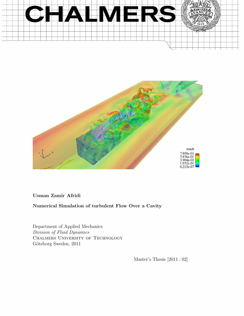
Usman Zamir Afridi
Numerical Simulation of turbulent Flow Over a Cavity
Department of Applied MechanicsDivision of Fluid DynamicsChalmers University of Technology
Goteborg Sweden, 2011
Master’s Thesis [2011 : 02]

2
Master’s Thesis 2011:
Numerical Simulation of turbulent Flow Over
a Cavity
Master’s Thesis
Usman Zamir Afridi
Department of Applied MechanicsDivision of Fluid Dynamics
Chalmers University of Technology
Goteborg, Sweden, 2011
3
Numerical Simulation of turbulent Flow Over a CavityMaster’s ThesisUsman Zamir Afridi
c© Usman Zamir Afridi, 2011
Master’s Thesis 2011:ISSN: 1652-8557
Department of Applied Mechanics,Division of Fluid DynamicsChalmers University of TechnologySe-412 96 Goteborg, SwedenPhone +46-(0)31-7721400Fax: +46-(0)31-180976
Printed at Chalmers ReproserviceGoteborg, Sweden 2011
Usman Zamir AfridiMaster’s Thesis
byUsman Zamir [email protected]
Department of Applied MechanicsDivision of Fluid Dynamics
Chalmers University of Technology
Abstract
Cavity flow and control of these flows have been of great importance formilitary as well as civil applications. Modern aircraft with internal carriageof weapon require active flow control techniques to ensure the structural in-tegrity by limiting the open bay acoustic resonance and efficient payload de-ployment. To implement these techniques it is important to understand theflow features and identify the source of resonance. Detached Eddy Simulation(DES) is carried out for subsonic flow (M = 0.85) over a three dimensionalcavity with Reynolds number based of cavity length equal to 7 × 10⁶. Agood comparison with the available experimental data for the similar con-figuration validates the DES results. Special attention is paid towards theprediction of unsteady pressure fluctuations and mixing layer and the result-ing tonal modes due to their interaction. Furthermore, the instantaneousand mean flow structures inside the cavity are compared with the availableLarge Eddy Simulation (LES) data, showing a good agreement with slightdeviation at the leading edge of the cavity. The Sound Pressure Level (SPL)comparison on cavity floor points show a good match between DES and ex-perimental results and also capturing the tonal modes. The Overall SoundPressure (OASPL) distribution is slightly overestimated (with maximum dif-ference equal to 1.5dB) by the DES. It is also observed that the self sustainedoscillations related to the tonal modes are independent of the stream-wiselocation in the cavity. The correlation analysis of the cavity floor points re-veal that the low frequencies are more correlated to the pressure fluctuationsin these locations.
Keywords:Cavity flow, Detached Eddy Simulation (DES), Computational Fluid Dy-
namics (CFD), Sound Pressure Level (SPL), Aeroacoustics, correlation
5

6

Acknowledgement
I would like to thank:My supervisors, Professor Lars Davidson and Shia-Hui Peng, for their
guidance and great support through their availability and dynamic discus-sions throughout this work. It was only their persistant support and patiencethat made it possible for be to carry out this work.
And, of course, all the people at the Department for their help and sup-port especially Bestian Nebensfur for providing me ahead start with the Edgeand assitance in postprocessing the results by sharing tips and tricks. I wouldlike to appretiate Huadong for taking me though the aeroacoustic part andSebastian Arvidson for providing a deeper insigh into the parallel processingand CFD methods in general and in Edge in particular.
Last but not the least i would like to thank my family for believeing inme and making it possible for me to persue my dream of higher education.I would especially thank my wife for her support and love during my thesiswork.
I would like to express my gratitude to QinetiQ for their experimentaldata and Lionel Larcheveque for LES results for comparision.
7

Nomenclature
Upper-case Roman
Cb1, Cb2, Cw1 Turbulence model constantsCp Specific heat at constant pressureCv Specific heat at constant pressureM Mach NumberP PressurePr Prandle numberR Gas constantRe Reynolds numberS Local deformation rateS∗ij Trace-less viscous strainT TemperatureU Velocity(L, T, U) Length, width and height of cavity respectively
Lower-case Roman
d Distance to the closest wall
d Turbulent length scalee Internal energyeo Total energyfn Frequency (nth Rossiter Mode)fν2 Wall dampinf functionsk Turbulent kinetic energyn Number of modeui Cartesian components of velocity vectorxi Cartesian coordinate vector componentp Pressureq Heat fluxt Timey Distance to the wall
Upper-case Greek
∆t Time step size∆x, ∆y, ∆z Streamwise, normal and spanwise mesh spacings
8
Ω Mean vorticity tensor
Lower-case Greek
δ Turbulent inflow boundary layer thicknessγ Empirical constant in Rossiter Formulaκ Von Karman constant, empirical constant in Rossiter formulaλ Thermal diffusion rateµ Dynamic viscosityν Kinematic eddy viscosity parameterρ Densityτij Viscous stress tensorτw Wall shear stress
Abbreviations
BISPL Band Integrated Sound Pressure LevelBL Boundary LayerCFD Computational Fluid DynamicsCFL Courant, Friedrichs and Lewy numberDES Detached Eddy SimulationDHIT Decaying Homogenous Isotropic TurbulenceDNS Direct Numerical SimulationEARSM Explicit Algebraic Reynolds Stress ModelOASPL Overall Sound Pressure LevelPSD Power Spectrun DensityRANS Reynolds-averaged Navier-StokesSA Spalart Allmaras (model)SGS Sub-Grid-ScaleSPL Sound Pressure LevelSST Shear Stress TransportURANS Unsteady Reynolds-averaged Navier-Stokes
subscripts
δ Quantity based on half channel-widthi Direction, node numberij Tensor indices∞ Freestream
superscripts
9

Ensemble average quatitiy˜ Favre-filtered ensemble average quatitiy′ Fluctuating component (reynold averaging)“ Fluctuating component (favre averaging)y+ =ypu
∗/ν
10
Contents
Abstract 5
Acknowledgement 7
Nomenclature 8
1 Introduction 11.1 Purpose . . . . . . . . . . . . . . . . . . . . . . . . . . . . . . 21.2 Limitations . . . . . . . . . . . . . . . . . . . . . . . . . . . . 2
2 Cavity Flow 52.1 Introduction . . . . . . . . . . . . . . . . . . . . . . . . . . . . 52.2 Noise Generation . . . . . . . . . . . . . . . . . . . . . . . . . 52.3 Classification of cavity . . . . . . . . . . . . . . . . . . . . . . 6
2.3.1 Classification based on L/D . . . . . . . . . . . . . . . 62.3.2 Classification based on L/W . . . . . . . . . . . . . . . 72.3.3 Classification based on flow phenomenon . . . . . . . . 7
2.4 Cavity Flow Properties . . . . . . . . . . . . . . . . . . . . . . 102.4.1 Mach Number Effects . . . . . . . . . . . . . . . . . . . 112.4.2 Boundary Layer Thickness (L/δ) . . . . . . . . . . . . 112.4.3 Pressure Spectra . . . . . . . . . . . . . . . . . . . . . 112.4.4 Rossiter Modes . . . . . . . . . . . . . . . . . . . . . . 12
3 Turbulence Modeling 153.1 Introduction . . . . . . . . . . . . . . . . . . . . . . . . . . . . 153.2 Governing Equation . . . . . . . . . . . . . . . . . . . . . . . . 15
3.2.1 Fluid Modeling . . . . . . . . . . . . . . . . . . . . . . 173.2.2 Time average Navier Stokes . . . . . . . . . . . . . . . 17
3.3 Turbulence Models . . . . . . . . . . . . . . . . . . . . . . . . 183.3.1 Close Form of Favre average Navier Stokes . . . . . . . 193.3.2 Spalart Allmaras One-equation model . . . . . . . . . . 22
11
3.3.3 Wilcox Standard k − ω turbulence model . . . . . . . . 233.3.4 SST Menter k − ω turbulence model . . . . . . . . . . 243.3.5 Explicit Algebraic Reynolds Stress Models (EARSM) . 25
3.4 Spalart-Allmaras DES Model . . . . . . . . . . . . . . . . . . 28
4 Simulation Methods 294.1 The Unstructured CFD Solver Edge . . . . . . . . . . . . . . . 29
4.1.1 Geometrical Considerations . . . . . . . . . . . . . . . 304.2 Boundary Condition . . . . . . . . . . . . . . . . . . . . . . . 31
4.2.1 Wall Boundary Condition . . . . . . . . . . . . . . . . 324.2.2 Symmetry Condition . . . . . . . . . . . . . . . . . . . 334.2.3 Farfield (Weak Characteristic) . . . . . . . . . . . . . . 33
4.3 Running a Computation With Edge . . . . . . . . . . . . . . . 334.3.1 Edge Files . . . . . . . . . . . . . . . . . . . . . . . . . 334.3.2 Grid . . . . . . . . . . . . . . . . . . . . . . . . . . . . 344.3.3 Edge Parameters . . . . . . . . . . . . . . . . . . . . . 344.3.4 Numerical Scheme . . . . . . . . . . . . . . . . . . . . 344.3.5 Boundary conditions . . . . . . . . . . . . . . . . . . . 354.3.6 Time Integration . . . . . . . . . . . . . . . . . . . . . 35
4.4 The Computational Set-up . . . . . . . . . . . . . . . . . . . . 35
5 Results and Discussion 395.1 2D Results . . . . . . . . . . . . . . . . . . . . . . . . . . . . . 39
5.1.1 Computational setup . . . . . . . . . . . . . . . . . . . 395.1.2 Summary of Results . . . . . . . . . . . . . . . . . . . 40
5.2 3D Results . . . . . . . . . . . . . . . . . . . . . . . . . . . . . 415.2.1 Mean Flow Comparison . . . . . . . . . . . . . . . . . 415.2.2 Pressure Oscillations . . . . . . . . . . . . . . . . . . . 455.2.3 Pressure Correlations . . . . . . . . . . . . . . . . . . . 48
6 Conclusion and Outlook 576.1 Conclusion and Outlook . . . . . . . . . . . . . . . . . . . . . 57
12
Chapter 1
Introduction
Cavity flows phenomenon have been of great interest in a variety of engi-neering applications, which can be observed, for example in the landing-gearwell in the deployment at landing and takeoff of aircraft, weapon bay of fight-ers, window open conditions in automobile industry, separation between twoconsecutive bogies of trains and depressions in hull of ships and sub-marines.
Cavity flows in aeronautic applications have been extensively studied bothexperimentally and computationally. With the purpose of reducing the radarvisibility and improve the aerodynamic performance. In addition, cavity flowresulting from landing-gear box during takeoff and landing has been regardedas being one of the major contributors of airframe noise due to extensivepressure fluctuations. Along with that, extensive pressure fluctuations mayfurther lead to structural fatigue and damaging the structure and the avionicshoused in the cavity.
Apart from the importance of the cavity flow in a variety of applications,the sophisticated flow physics of cavity flows has always attracted people tostudy it. The Study by Roshko [1] was one of the pioneering work. Themain focus was laid on the strong self-sustained oscillations that arise fromthe vorticity-pressure feedback loop encountered in this kind of flow. Flowinside cavities is distinguished by boundary layer separation, shear layer in-stabilities, unsteadiness and vortical flow motion. Due to these flow features,the cavity flow is prone to aero-acoustic resonance. The acoustic tones gen-erated are often regarded as a result of interaction between shear layer andthe aft wall on which it impinges [2]. Another major contribution to cav-ity flow study is the formula proposed by Rossiter[3]. The resonant loopof mixing-layer vortices moving downstream with velocity κU∞ and pressurewaves traveling upstream inside the cavity with the speed of sound, results indiscrete tonal modes, of which the frequency can be approximately calculatedby using the Rossiter formula (Eq. 2.1).
1
The present study concerns of numerical simulations of a generic config-uration weapon-bay. The rectangular cavity has the dimensions of L = 20inches in length, D = 4 inches in diameter and W = 4 inches in width, giv-ing an aspect ratio of L : D : W = 4 : 1 : 1. The cavity was analyzed withfreestream flow conditions of M∞ = 0.85, P∞ = 6.21 × 10⁴, T∞ = 266.53Kand Re = 13.47 × 10⁶ per meter.
1.1 Purpose
The purpose of this project is to explain the cavity flow physics by meansof accurate flow simulations and to understand how these simulations can beimproved for solving cavity flows. The main focus is laid on resolving thecomplex flow structures, prediction of pressure fluctuations and the gener-ated acoustic tones inside the cavity. Furthermore, to add to the availabledatabase of extensive work already carried out over the M219 − cavity ina previous EU DESider project [4]. This will be useful in examination ofturbulence modeling of this kind of flows. Based on the simulation, anotherimportant objective is to interpret the interaction of acoustic tones with theshear layer instabilities. It is expected the analysis may provide implicationsfor future work on flow control of cavity flows.
1.2 Limitations
With turbulence resolving simulations using DES and other hybrid RANS-LES methods, the requirement on computational resources is further high.The DES computation carried out was computationally heavy requiring longtime to run, therefore, there was little flexibility in trying different set-tings/turbulence models. Also the data storage required to store the flowsolution at each timestep for entire domain further increases the simulationtime, which might have been helpful in analyzing shear layer region moreextensively with a better insight to flow behavior in that particular region.
The computation started with 2D simulations using RANS. It was foundthat the Spalart-Allmaras and EARSM model showed acceptable conver-gence, whereas for the Menter SST k − ω and the Wilcox Standard k − ωturbulence model the simulation diverged. For URANS computations werealso showing divergence using the SST k − ω model. For the SA and theEARSM turbulence model, the unsteadiness in the flow was dampened outand the solution converges to a steady state.
2

With turbulence resolving simulations using DES and other hybrid RANS-LES methods, the requirement on computational resources is further high.
3

4
Chapter 2
Cavity Flow
2.1 Introduction
Cavity flow can be described as the interaction of different flow phe-nomenon, such as hydrodynamic instabilities, flow separation and recircu-lation, vortex motions, acoustic noise generation and wave propagation andaero-acoustic coupling related to the self-sustaining vorticity pressure feed-back. The aero-acoustic resonance is the aerodynamic noise generated andthe flow conditions in the cavity result in self sustaining oscillations, whichhave adverse affects on the integrity of the structure. In order to reducethe noise, it is important to understand the flow features and thus developmethods to control the flow. Cavity flow has been studied experimentallyand numerically.
2.2 Noise Generation
One of the first researchers who carried out experimental work on cavityflow was Rossiter[3]. In his experiments he tested different geometries and bystudying the shadowgraphs, identifying the pressure waves and flow patternhe came up with the description of the feedback mechanism. The source forthe aerodynamic loads is due to the natural flow instabilities in the cavity.The shear layer develops as the freestream flow separates from the leadingedge of the cavity. The shear layer breaks down further downstream, andthe emerging vortex shedding impinging on the rear wall results in pressurewaves. These pressure waves travel upstream and interact with the mixinglayer. This interaction of the pressure wave with the Kelvin-Helmontz typeshear layer instability leads to a self sustained mechanism, inducing acousticnoise as shown schematically in Fig. 2.1. This process forms a feed back loop
5

and, upon the cavity geometry, tonal noise may generate due to unsteadypressure modes.
Figure 2.1: Schematic view of the self-sustained pressure oscillations
2.3 Classification of cavity
Depending upon the applications different kinds of cavities are used,which are classified on the basis of cavity geometry and the flow condition.Much experimental and numerical work have been carried out to study theaffects of different geometries [3] [5] [6] and to identify different types offlow patterns in the cavity [7] [8] [9]. Some of the basic classifications aredescribed below.
2.3.1 Classification based on L/D
One of the basic classification of cavities is deep and shallow cavities,based upon the aspect ratio (L/D), where L and D are the characteris-tic length and depth of the cavity respectively. Cavities with aspect ratiosmaller than one are categorized as deep cavities, whereas the one with as-pect ratio larger than one are referred to as shallow cavities. On the otherhand, Rossiter through his experimental observations described cavities withL/D < 4 as deep cavities and vice versa. The deep cavities are associatedwith periodic and energetic tones, while in shallow cavities broadband noise(i.e. the random components) with higher amplitudes are generated.
6

2.3.2 Classification based on L/W
Several researchers have been analyzing the flow properties in the cavityunder the influence of varying dimensions. Cavity with L/W < 1 is referredas three-dimensional and if L/W > 1 it is classified as two-dimensional.Block [10] was the first who classified the cavity on the basis of length-to-width ratio (L/W ). Ahuja and Mendoza [6] came up with the similarobservations/results. They found that the frequency of the peak is unaffectedby the change in cavity width, but there is approximately 15 dB reduction inoverall sound pressure level (OASPL) for 3D cavities. Furthermore, Dismile[5] observed that the number of tones of dominant frequencies increases asL/W decreases.
2.3.3 Classification based on flow phenomenon
Several factors involved in cavity flow may significantly impact the cavityflow properties. These include geometric variables like L/W , L/D and flowparameters like free-stream Mach number. Based on the flow features, cavityflows have usually been classified into three different types, namely, Open,closed and transitional flow.
Closed flow
As shown in Fig. 2.2,a closed cavity flow is formed in case of cavitylength-to-depth ratio larger than 13 [7]. In this type of flow the shear layergrowing from the leading edge of the cavity impinges on the cavity floor,detaches further downstream from the cavity floor and finally passes overthe cavity rear wall, resulting in two recirculation regions in the front andrear part of the cavity, one before the flow impinges on the cavity floor andthe second one after the detachment, as shown in Fig. 2.2.
Figure 2.2: Sub-sonic closed cavity flow
For a closed cavity flow at supersonic conditions, an expansion wave isobserved at the front wall and rear wall, where the flow turns away from itself
7
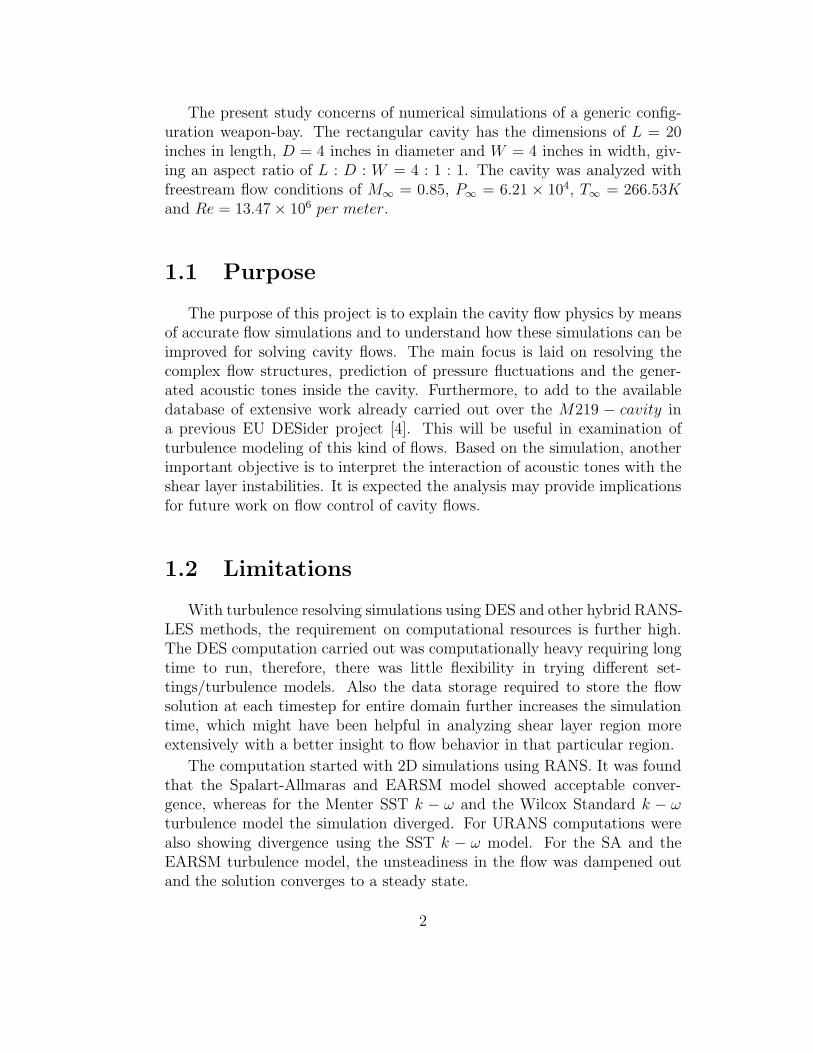
around the corner. A shock is generated at the location of flow attachmentand detachment from the cavity floor, as illustrated in Fig. 2.3. The Cp
behavior resulting from the expansion and shock waves is shown in Fig. 2.3.
Figure 2.3: Super-sonic closed cavity flow with pressure distribution on cavityfloor
Open Flow
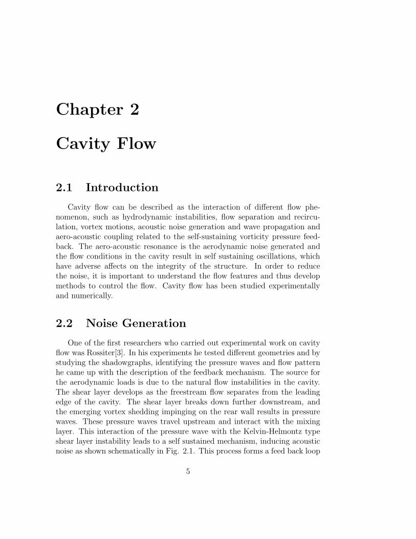
Open flow phenomenon is observed in the cavity with the length-to-depthratio less than 10.[11]. In this case the shear layer does not impinge on thecavity floor and Cp exhibits a rather constant behavior except close to rearwall where the shear layer impinges. The open cavity flow pattern is shownin Fig. 2.4.
Figure 2.4: Sub-sonic open cavity flow
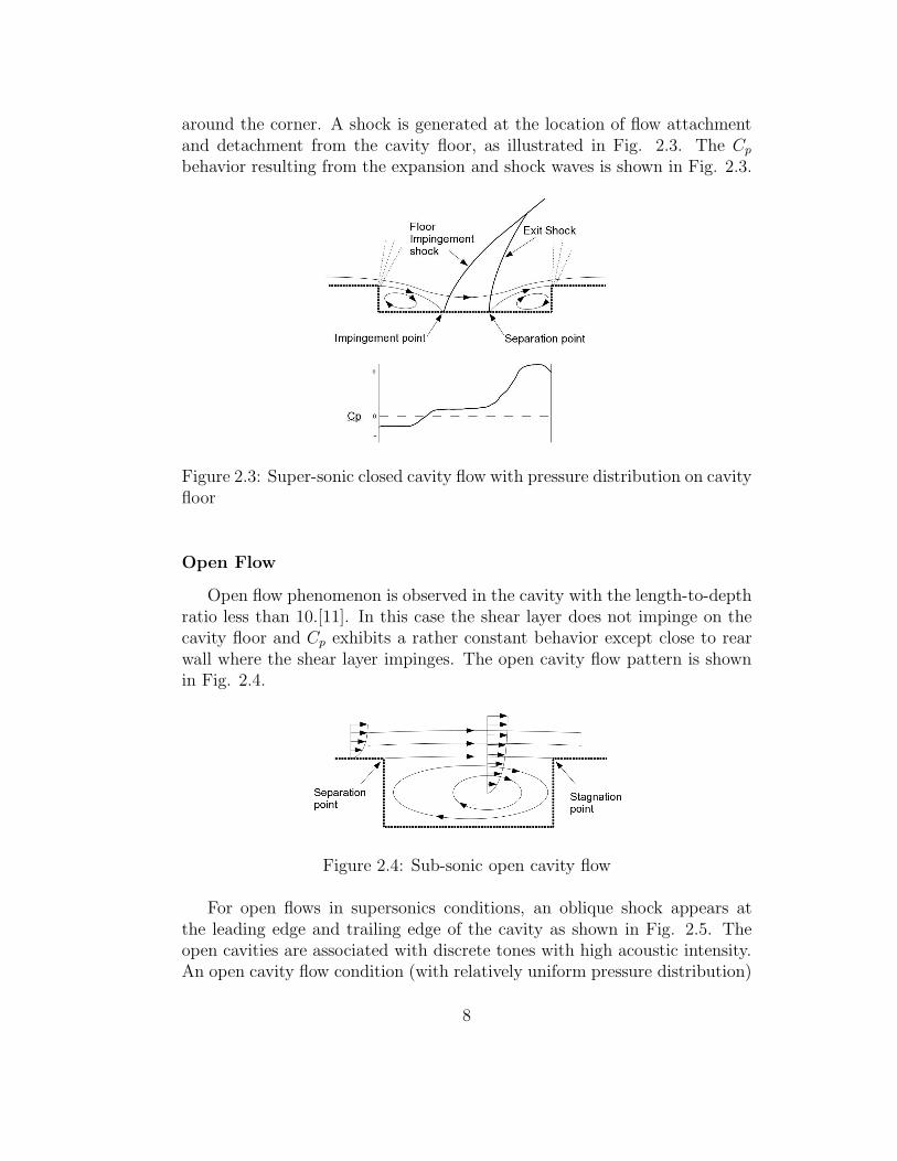
For open flows in supersonics conditions, an oblique shock appears atthe leading edge and trailing edge of the cavity as shown in Fig. 2.5. Theopen cavities are associated with discrete tones with high acoustic intensity.An open cavity flow condition (with relatively uniform pressure distribution)
8
provides favorable conditions for cargo separation for weapon-bay type cavity[7].
Figure 2.5: Super-sonic open cavity flow with pressure distribution on cavityfloor
Transitional flow
The cavity is said to be open when the reattachment of the shear layertakes place at the rear edge and in case of reattachment point on the cavityfloor, it is called closed cavity. When the two states occur randomly, the flowis called transitional. This kind of behavior is observed in cavities with thelength-to-depth ratio of 10 < L/D < 13 [11]. The transitional flow featuresare strongly dependent on the free-stream Mach number. For subsonic flowconditions the transition is a smooth process. At supersonic flow conditionsit is a two-step process with abrupt changes in flow characteristics. Thetwo stages are classified further as transitional open and transitional closedcavities based on the location of attached and detached shocks.
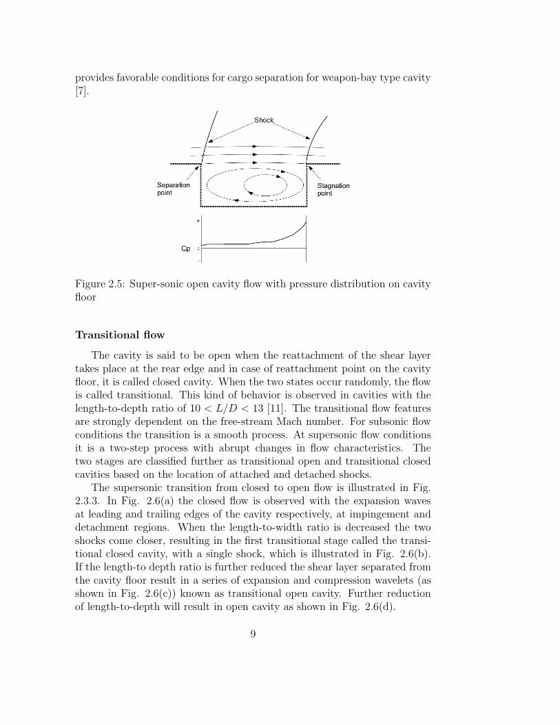
The supersonic transition from closed to open flow is illustrated in Fig.2.3.3. In Fig. 2.6(a) the closed flow is observed with the expansion wavesat leading and trailing edges of the cavity respectively, at impingement anddetachment regions. When the length-to-width ratio is decreased the twoshocks come closer, resulting in the first transitional stage called the transi-tional closed cavity, with a single shock, which is illustrated in Fig. 2.6(b).If the length-to depth ratio is further reduced the shear layer separated fromthe cavity floor result in a series of expansion and compression wavelets (asshown in Fig. 2.6(c)) known as transitional open cavity. Further reductionof length-to-depth will result in open cavity as shown in Fig. 2.6(d).
9
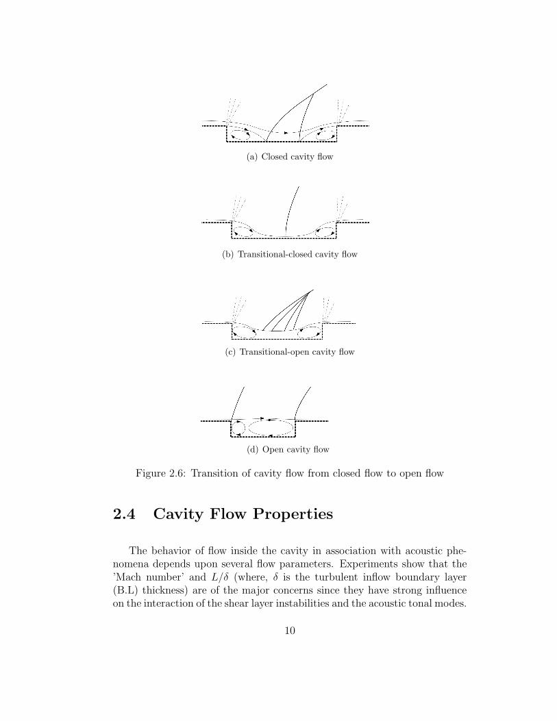
(a) Closed cavity flow
(b) Transitional-closed cavity flow
(c) Transitional-open cavity flow
(d) Open cavity flow
Figure 2.6: Transition of cavity flow from closed flow to open flow
2.4 Cavity Flow Properties
The behavior of flow inside the cavity in association with acoustic phe-nomena depends upon several flow parameters. Experiments show that the’Mach number’ and L/δ (where, δ is the turbulent inflow boundary layer(B.L) thickness) are of the major concerns since they have strong influenceon the interaction of the shear layer instabilities and the acoustic tonal modes.
10

2.4.1 Mach Number Effects
Acoustic tones inside a cavity activate when a certain Mach number isachieved. With an increasing mach number, the cavity flow transits fromthe shear layer mode to wake mode. In shear layer mode, the dominantfrequency of the pressure fluctuations seems to oscillate with increasing Machnumber. Colonious et al. [12] by means of analysis of the Direct NumericalSimulation (DNS) data, observed that for the range of Mach = 0.4 to 0.8,the fundamental frequencies are almost independent of the Mach number.The experimental study by Gates et al. [13] further certified that the modalamplitude is independent of the Mach number.
2.4.2 Boundary Layer Thickness (L/δ)
Incoming boundary layer thickness plays an important role in the cavityflow mechanism. Generally the boundary layer thickness is used to normalizethe characteristic lengths (in this case length and depth of the cavity) foranalysis and comparison, usually with L/δ or D/δ. Sarohia and Massiar[14] in their studies of the boundary layer effect observed that there existsa critical L/δ value at which steady shear layer transits to unsteady shearlayer. Rockwell and Nadascher [15] also observed a similar phenomenon andindicated a critical value of L/δ beyond which a sudden increase occurs inthe dominant frequencies, similar to the effect of Mach number in shear-layermode.
2.4.3 Pressure Spectra
The sound waves travel as pressure waves generated by the unsteadyflow field. The generation and propagation of these acoustic waves havealways been of interest in aeronautic and other industrial applications. Thegoverning equations for the aeroacoustic wave generation and propagationare the same as a fluid dynamics. One of the main problems while using thefluid dynamics equations is that the sound waves carry a very low energyas compared to the fluid flow itself. Therefore, resolving these sound wavesnumerically and predicting the propagation is quite a challenge. A typicalpressure spectrum for unsteady cavity flow comprises of random and periodicpressure fluctuations, which vary in magnitude depending upon the type offlow. In case of closed cavity, the pressure spectrum is dominated by randompressure fluctuations. On the other hand, the open cavity flow is dominatedby periodic pressure oscillations with less random fluctuations. A typicalSPL spectra for open and closed cavity flow are shown in Fig. 2.7.
11
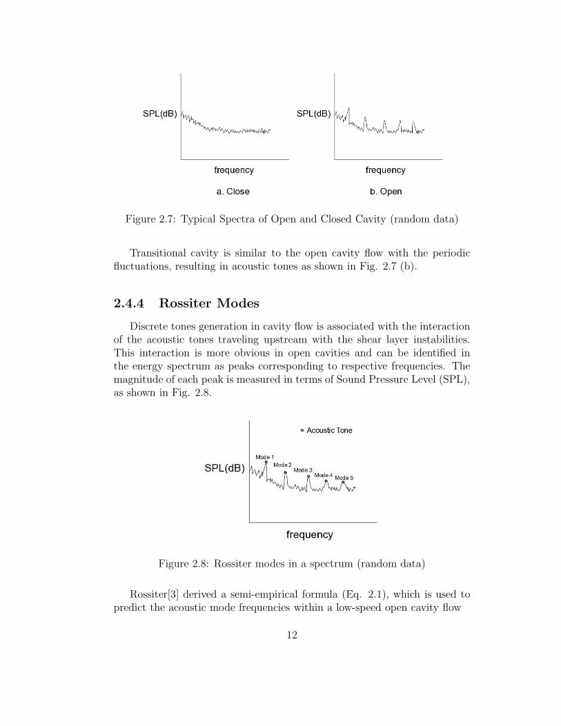
Figure 2.7: Typical Spectra of Open and Closed Cavity (random data)
Transitional cavity is similar to the open cavity flow with the periodicfluctuations, resulting in acoustic tones as shown in Fig. 2.7 (b).
2.4.4 Rossiter Modes
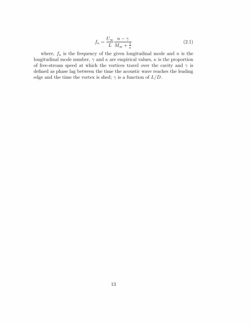
Discrete tones generation in cavity flow is associated with the interactionof the acoustic tones traveling upstream with the shear layer instabilities.This interaction is more obvious in open cavities and can be identified inthe energy spectrum as peaks corresponding to respective frequencies. Themagnitude of each peak is measured in terms of Sound Pressure Level (SPL),as shown in Fig. 2.8.
Figure 2.8: Rossiter modes in a spectrum (random data)
Rossiter[3] derived a semi-empirical formula (Eq. 2.1), which is used topredict the acoustic mode frequencies within a low-speed open cavity flow
12
fn =U∞
L
n − γ
M∞ + 1κ
(2.1)
where, fn is the frequency of the given longitudinal mode and n is thelongitudinal mode number, γ and κ are empirical values, κ is the proportionof free-stream speed at which the vortices travel over the cavity and γ isdefined as phase lag between the time the acoustic wave reaches the leadingedge and the time the vortex is shed; γ is a function of L/D.
13

14

Chapter 3
Turbulence Modeling
3.1 Introduction
Flow separations are of great importance especially in aeronautic appli-cations. To predict this aerodynamic flow, classical RANS models are notcapable of capturing the flow details accurately. Therefore, approaches likeDetached Eddy Simulation (DES) and Large Eddy Simulation (LES) areapplied to capture the flow properties more accurately. LES being more ex-pensive numerically, DES is a reasonable choice, which is a combination ofLES and RANS. One of the motivation behind development of such methodsis for aeronautical applications. Among the other researchers, some initialwork in this regard was carried out by Spalart et al.,(1997) [16]. The ideawas to use the fine tuned RANS model in the attached boundary layer andimplement LES in the separated flow region with large eddies and detachedfrom the geometry, which cannot be captured with the traditional RANSmodel.
For flows with higher Reynolds number, pure LES requires a great deal ofrefinement near the wall regions, resulting in huge grid size. DES on the otherhand uses RANS mode in the wall boundary coupled with the LES mode inthe off-wall region and regions where flow is “detached“ from wall surface.RANS being computationally efficient and LES computationally more accu-rate, DES is a reasonably well combination to get acceptable accuracy withcomputational efficiency.
3.2 Governing Equation
The cavity flow under the present conditions is compressible. Therefore,compressible form of the continuity, momentum and energy equation are
15
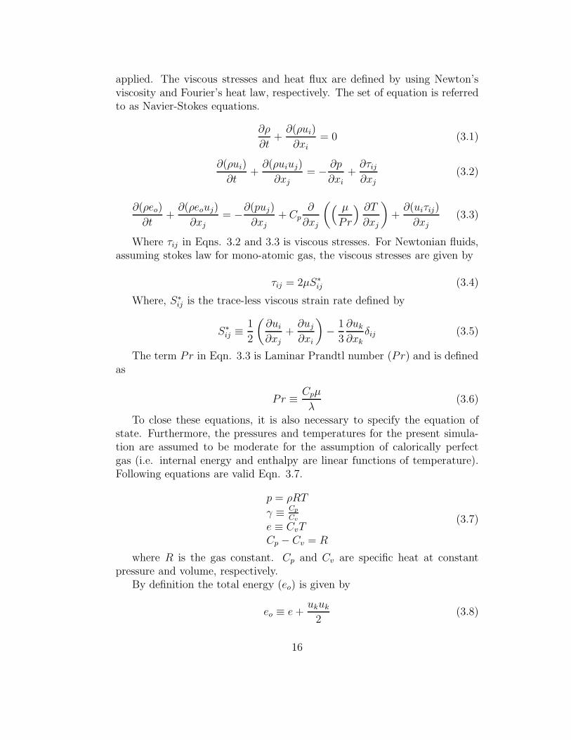
applied. The viscous stresses and heat flux are defined by using Newton’sviscosity and Fourier’s heat law, respectively. The set of equation is referredto as Navier-Stokes equations.
∂ρ
∂t+
∂(ρui)
∂xi= 0 (3.1)
∂(ρui)
∂t+
∂(ρuiuj)
∂xj= − ∂p
∂xi+
∂τij
∂xj(3.2)
∂(ρeo)
∂t+
∂(ρeouj)
∂xj= −∂(puj)
∂xj+ Cp
∂
∂xj
(( µ
Pr
) ∂T
∂xj
)+
∂(uiτij)
∂xj(3.3)
Where τij in Eqns. 3.2 and 3.3 is viscous stresses. For Newtonian fluids,assuming stokes law for mono-atomic gas, the viscous stresses are given by
τij = 2µS∗ij (3.4)
Where, S∗ij is the trace-less viscous strain rate defined by
S∗ij ≡
1
2
(∂ui
∂xj+
∂uj
∂xi
)− 1
3
∂uk
∂xkδij (3.5)
The term Pr in Eqn. 3.3 is Laminar Prandtl number (Pr) and is definedas
Pr ≡ Cpµ
λ(3.6)
To close these equations, it is also necessary to specify the equation ofstate. Furthermore, the pressures and temperatures for the present simula-tion are assumed to be moderate for the assumption of calorically perfectgas (i.e. internal energy and enthalpy are linear functions of temperature).Following equations are valid Eqn. 3.7.
p = ρRT
γ ≡ Cp
Cv
e ≡ CvTCp − Cv = R
(3.7)
where R is the gas constant. Cp and Cv are specific heat at constantpressure and volume, respectively.
By definition the total energy (eo) is given by
eo ≡ e +ukuk
2(3.8)
16

3.2.1 Fluid Modeling
For fluid modeling, as discussed above, the perfect gas law is used
p = ρrT (3.9)
where r is the gas constant for perfect gas and is defined as:
r =R
M(3.10)
Where R is universal gas constant and M is the molecular weight of theperfect gas.
Calorically Perfect GasFor low temperature condition flow, where vibrational and electronic modesare not present, the internal energy of the gas is proportional to temperature.This means γ, Cp, Cv and R are constants. For moderate speed aerodynamicsthe assumption of calorically perfect gas stands valid and r and Cp are relatedas:
r =γ − 1
γCp (3.11)
Thermally Perfect GasFor higher temperature flows, we treat the flow as thermally perfect gas. Inthis case the internal energy is varied by excitation of the transitional, rota-tional, vibrational and electronic modes of the gas molecules and no chemicalreaction or ionization occur, meaning internal energy is only function of tem-perature. Therefore, it can be treated as thermally perfect. In this casethe specific heats are now functions of Temperature. Thermally perfect gasassumption is also valid for mixing of different thermally perfect gases. Foreach gas and its fraction of total density, an equation is solved.
3.2.2 Time average Navier Stokes
For turbulence the flow quantities are decomposed into two parts thetime-averaged and fluctuating quantities. In order to get the average formof the governing equation, the following time averaging methods are used.
For any dependent variable φ,Reynolds Averaging, also known as classical time averaging, reads
φ′ ≡ φ − φ
φ ≡ 1T
∫T
φ(t) dt(3.12)
17
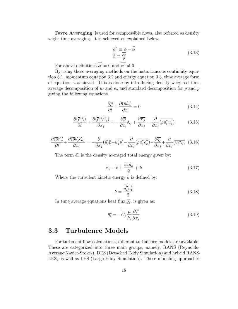
Favre Averaging, is used for compressible flows, also referred as densitywight time averaging. It is achieved as explained below.
φ′′ ≡ φ − φ
φ ≡ ρφρ
(3.13)
For above definitions φ′ = 0 and φ′′ 6= 0By using these averaging methods on the instantaneous continuity equa-
tion 3.1, momentum equation 3.2 and energy equation 3.3, time average formof equation is achieved. This is done by introducing density weighted timeaverage decomposition of ui and eo and standard decomposition for ρ and pgiving the following equations.
∂ρ
∂t+
∂(ρui)
∂xi
= 0 (3.14)
∂(ρui)
∂t+
∂(ρuiuj)
∂xj
= − ∂p
∂xi
δij +∂τij
∂xj
− ∂
∂xj
(ρu′′
i u′′
j ) (3.15)
∂(ρeo)
∂t+
∂(ρuj eo)
∂xj
= − ∂
∂xj
(ujp+u′′
j p)− ∂
∂xj
(ρu′′
j e′′
o)−∂qj
∂xj
+∂
∂xj
(uiτij) (3.16)
The term eo is the density averaged total energy given by:
eo ≡ e +ukuk
2+ k (3.17)
Where the turbulent kinetic energy k is defined by:
k =u
′′
ku′′
k
2(3.18)
In time average equations heat flux,qj , is given as:
qj = −Cpµ
Pr
∂T
∂xj
(3.19)
3.3 Turbulence Models
For turbulent flow calculations, different turbulence models are available.These are categorized into three main groups, namely, RANS (Reynolds-Average Navier-Stokes), DES (Detached Eddy Simulation) and hybrid RANS-LES, as well as LES (Large Eddy Simulation). These modeling approaches
18

can be selected in the input file by setting ITURB = 2 for RANS, ITURB =3 for DES and hybrid RANS-LES and finally ITURB = 4 for LES model-ing. For each modeling approach, different turbulence models are availablefor selection. Depending upon type of flow features involved and desiredanalysis, the best suited turbulence model can be selected with the variableTURB MOD NAME in edge input file.
3.3.1 Close Form of Favre average Navier Stokes
The Eqns.3.14, 3.15 and 3.16 are referred as Favre averaged Navier Stokesequations. p, ui and eo are the primary solution variables. This group ofequations contains several unknown correlation terms and is an open set ofpartial differential equation. To solve this set of equations some correlationterms needs to be modeled to obtain the closed form of equation.
Approximation and modelling
The unknown terms are rewritten as following.
τij = τij + τ′′
ij (3.20)
u′′
j p + ρu′′
j e′′
o = Cpρu′′
j T + uiρu′′
i u′′
j +ρu
′′
j u′′
i u′′
i
2(3.21)
qj = −Cpµ
Pr
∂T
∂xj
= −Cpµ
Pr
∂T
∂xj
− Cpµ
Pr
∂T ′′
∂xj
(3.22)
uiτij = uiτij + u′′
i τij + uiτ′′
ij (3.23)
By inserting these terms in Favre averaged Navier Stokes equation gives.
∂ρ
∂t+
∂(ρui)
∂xi
= 0 (3.24)
∂(ρui)
∂t+
∂(ρuiuj)
∂xj= − ∂
∂xj
pδij − τij − tau
′′
ij︸︷︷︸2*
+ ρu′′
i u′′
j︸ ︷︷ ︸1*
(3.25)
19
∂(ρeo)
∂t+
∂(ρuj eo)
∂xj= − ∂
∂xj(ujp + Cpρu
′′
j T︸ ︷︷ ︸3*
+ uiρu′′
i u′′
j︸ ︷︷ ︸4*
+ρu
′′
j u′′
i u′′
i
2︸ ︷︷ ︸5*
−
Cpµ
Pr
∂T
∂xj− Cp
µ
Pr
∂T ′′
∂xj︸ ︷︷ ︸6*
−uiτij − u′′
i τij︸︷︷︸7*
− uiτ′′
ij︸︷︷︸8*
)
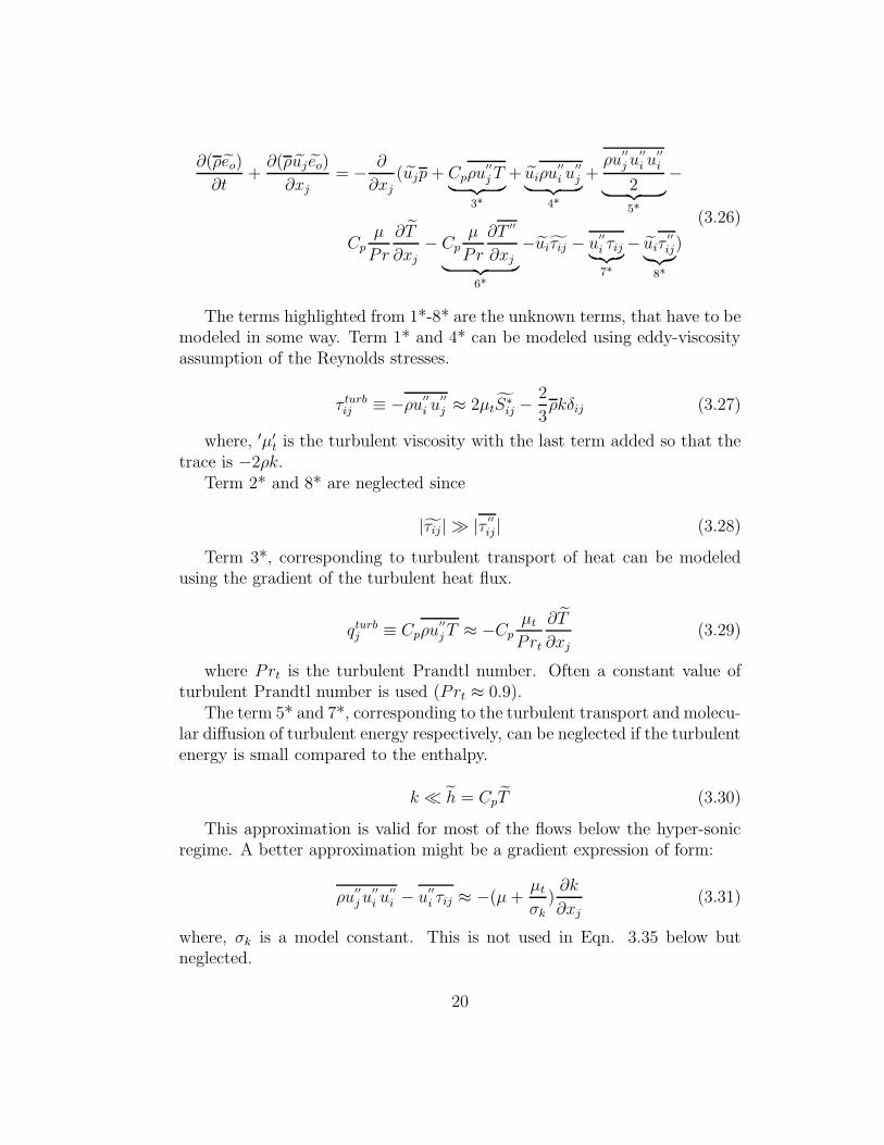
(3.26)
The terms highlighted from 1*-8* are the unknown terms, that have to bemodeled in some way. Term 1* and 4* can be modeled using eddy-viscosityassumption of the Reynolds stresses.
τ turbij ≡ −ρu
′′
i u′′
j ≈ 2µtS∗ij −
2
3ρkδij (3.27)
where, ′µ′t is the turbulent viscosity with the last term added so that the
trace is −2ρk.Term 2* and 8* are neglected since
|τij| ≫ |τ ′′
ij | (3.28)
Term 3*, corresponding to turbulent transport of heat can be modeledusing the gradient of the turbulent heat flux.
qturbj ≡ Cpρu
′′
j T ≈ −Cpµt
Prt
∂T
∂xj
(3.29)
where Prt is the turbulent Prandtl number. Often a constant value ofturbulent Prandtl number is used (Prt ≈ 0.9).
The term 5* and 7*, corresponding to the turbulent transport and molecu-lar diffusion of turbulent energy respectively, can be neglected if the turbulentenergy is small compared to the enthalpy.
k ≪ h = CpT (3.30)
This approximation is valid for most of the flows below the hyper-sonicregime. A better approximation might be a gradient expression of form:
ρu′′
j u′′
i u′′
i − u′′
i τij ≈ −(µ +µt
σk
)∂k
∂xj
(3.31)
where, σk is a model constant. This is not used in Eqn. 3.35 below butneglected.
20

Term 6* is an artifact from Favre averaging. It is related to the heat con-duction effects associated with temperature fluctuations. it can be neglectedif
| ∂2T
∂xj2 | ≫ |∂
2T ′′
∂xj2 | (3.32)
This is virtually true for all the flows and hence it is neglected.By applying all the approximations and assumptions the final closed form
of the Favre averaged Navier Stokes equation is achieved as following.
∂ρ
∂t+
∂ (ρui)
∂xi
= 0 (3.33)
∂(ρui)
∂t+
∂ (ρuiuj)
∂xj
= − ∂p
∂xj
δij +∂τTot
ij
∂xj
(3.34)
∂(ρeo)
∂t+
∂ρuj eo
∂xj= − ∂
∂xj
(ujp + qTot
j + uiτTotij
)(3.35)
where,
τTotij = τ lam
ij τ turbij (3.36)
τ lamij ≡ τij = µ
(∂ui
∂xj
+∂ui
∂xi
− 2
3
∂uk
∂xk
δij
)(3.37)
τ turbij ≡ −ρu
′′
i u′′
j ≈ µt
(∂ui
∂xj+
∂ui
∂xi− 2
3
∂uk
∂xkδij
)− 2
3ρkδij (3.38)
qTotj ≡ qlam
j + qturbj (3.39)
qlamj ≡ qj ≈ −Cp
µ
Pr
∂T
∂xj=
γ
γ − 1
µ
Pr
∂
∂xj
(p
ρ
)(3.40)
qturbj ≡ Cpρu
′′
j T ≈ −Cpµt
Prt
∂T
∂xj
=γ
γ − 1
µt
Prt
∂
∂xj
(p
ρ
)(3.41)
p = (γ − 1)ρ
(eo −
ukuk
2− k
)(3.42)
If a separate turbulence model is used to solve for µt, k and Prt, and gasdata is given for µ, γ and Pr than these equations form a closed set of partialdifferential equation which can be solved numerically.
21

3.3.2 Spalart Allmaras One-equation model
The model solves one transport equation for a quantity of “ν“ (kine-matic eddy viscosity parameter). The turbulence is characterized by thelength scales and the velocity scales, see ref: Spalart et al.,(1994)[17]. Themodel only solves for one property, additional information is needed. In one-equation model the length scale cannot be computed, but must be specifiedto determine the rate of dissipation of the transported turbulence quantity.the model is integrated all the way to the wall which requires a good res-olution of mesh normal to the wall surface (y+ ∼ 1). The (dynamic) eddyviscosity is related to ν by
µt = ρνfν1
fν1 = χ3
χ3+C3ν1
χ ∼= eνν
(3.43)
fν1 = fν1
(eνν
), which tends to unity for higher Reynolds numbers.
⇒ ν = νt and at wall fν1 −→ 0The Reynolds stresses are computed with
τij = −ρu′
iu′
j = 2µtSij = ρνfν1
(∂ui
∂xj
+∂uj
∂xi
)(3.44)
The transport equation for ν is as following:
∂(ρν)
∂t+
∂(ρνui)
∂xi
=1
σν
(∂
∂xi
((µ + ρν)
∂ν
∂xi
)+ Cb2ρ
∂ν
∂xj
∂ν
∂xj
)
+Cb1ρνΩ − Cw1ρ
(ν
d
)2
fw
(3.45)
where,
Ω = Ω +ν
(κy)2fν2 (3.46)
Ω =√
2ΩijΩij = mean vorticity
Ωij = 12
(∂ui
∂xj+
∂uj
∂xi
)= mean vorticity tensor
d = κyfν2 = fν2
(eνν
)
fw = fw
(eν
Ωκ2y2
)(3.47)
fν2 and fw are the wall damping functions. Inspection of destruction termreveal that κy (with y = distance to the wall) has been used as length scale.
22
The length scale κy also enters in the vorticity parameter Ω and is just equalto the mixing layer length.
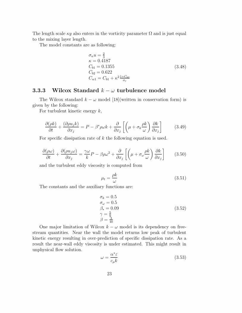
The model constants are as following:
σnu = 23
κ = 0.4187Cb1 = 0.1355Cb2 = 0.622Cw1 = Cb1 + κ2 1+Cb2
σν
(3.48)
3.3.3 Wilcox Standard k − ω turbulence model
The Wilcox standard k − ω model [18](written in conservation form) isgiven by the following:
For turbulent kinetic energy k,
∂(ρk)
∂t+
(∂ρujk)
∂xj= P − β∗ρωk +
∂
∂xj
[(µ + σk
ρk
ω
)∂k
∂xj
](3.49)
For specific dissipation rate of k the following equation is used.
∂(ρω)
∂t+
∂(ρujω)
∂xj=
γω
kP − βρω2 +
∂
∂xj
[(µ + σω
ρk
ω
)∂k
∂xj
](3.50)
and the turbulent eddy viscosity is computed from
µt =ρk
ω(3.51)
The constants and the auxiliary functions are:
σk = 0.5σω = 0.5β∗ = 0.09γ = 5
9
β = 340
(3.52)
One major limitation of Wilcox k − ω model is its dependency on free-stream quantities. Near the wall the model returns low peak of turbulentkinetic energy resulting in over-prediction of specific dissipation rate. As aresult the near-wall eddy viscosity is under estimated. This might result inunphysical flow solution.
ω =α∗ε
cµk(3.53)
23

3.3.4 SST Menter k − ω turbulence model
The SST Menter k −ω model [19] is developed to resolve the free streamdependency problem resulting in unphysical flow solution. To achieve thisa cross diffusion term is added to the k − ω model. The model uses k − εformulation in the outer part of the boundary layer and uses the Wilcox k−ωmodel near the wall part of the boundary layer. The transformation fromk−ε to k−ω is achieved by introduction of cross diffusion term and modifiedcoefficients which are implemented by a blending function.
The closed form of the SST Menter k − ω model is as following.
For turbulent kinetic energy k,
∂(ρk)
∂t+
∂(ρujk)
∂xj= P − β∗ρωk +
∂
∂xj
[(µ + σkµt)
∂k
∂xj
](3.54)
For specific dissipation rate of k,
∂(ρω)
∂t+
∂(ρujω)
∂xj=
γ
νtP − βρω2 +
∂
∂xj
[(µ + σωµt)
∂ω
∂xj
]+
2(1 − F1)ρσω2
ω
∂k
∂xj
∂ω
∂xj
(3.55)
Where kinematic eddy viscosity is given as
µt =ρa1k
max(a1ω, ΩF2)(3.56)
and
P = τij∂ui
∂xj
τij = µt
(2Sij − 2
3∂uk
∂xkδij
)− 2
3ρkδij
Sij = 12
(∂ui
∂xj+
∂uj
∂xi
) (3.57)
Each constant is a mix of inner and outer constant blended by the function
φ = F1φ1 + (1 − F1)φ2 (3.58)
where, φ1 and φ2 represents the inner and outer constants respectively.Additionalrelations are
24
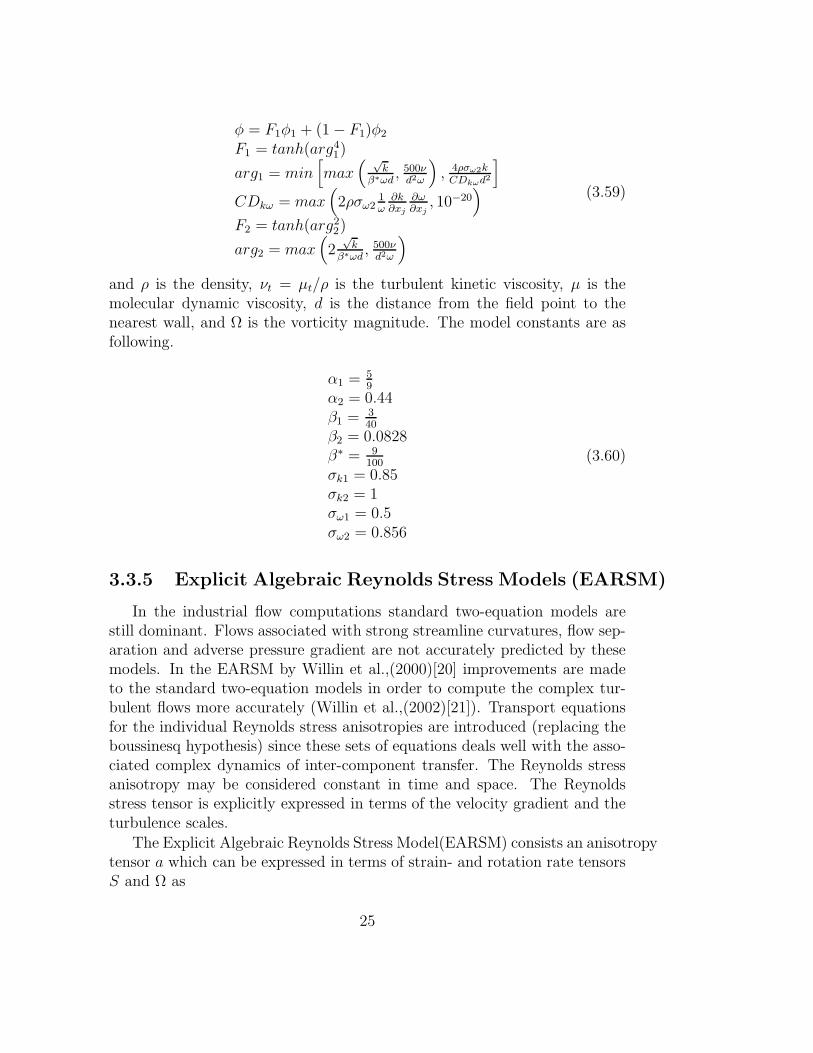
φ = F1φ1 + (1 − F1)φ2
F1 = tanh(arg41)
arg1 = min[max
( √k
β∗ωd, 500ν
d2ω
), 4ρσω2k
CDkωd2
]
CDkω = max(2ρσω2
1ω
∂k∂xj
∂ω∂xj
, 10−20)
F2 = tanh(arg22)
arg2 = max(2
√k
β∗ωd, 500ν
d2ω
)
(3.59)
and ρ is the density, νt = µt/ρ is the turbulent kinetic viscosity, µ is themolecular dynamic viscosity, d is the distance from the field point to thenearest wall, and Ω is the vorticity magnitude. The model constants are asfollowing.
α1 = 59
α2 = 0.44β1 = 3
40
β2 = 0.0828β∗ = 9
100
σk1 = 0.85σk2 = 1σω1 = 0.5σω2 = 0.856
(3.60)
3.3.5 Explicit Algebraic Reynolds Stress Models (EARSM)
In the industrial flow computations standard two-equation models arestill dominant. Flows associated with strong streamline curvatures, flow sep-aration and adverse pressure gradient are not accurately predicted by thesemodels. In the EARSM by Willin et al.,(2000)[20] improvements are madeto the standard two-equation models in order to compute the complex tur-bulent flows more accurately (Willin et al.,(2002)[21]). Transport equationsfor the individual Reynolds stress anisotropies are introduced (replacing theboussinesq hypothesis) since these sets of equations deals well with the asso-ciated complex dynamics of inter-component transfer. The Reynolds stressanisotropy may be considered constant in time and space. The Reynoldsstress tensor is explicitly expressed in terms of the velocity gradient and theturbulence scales.
The Explicit Algebraic Reynolds Stress Model(EARSM) consists an anisotropytensor a which can be expressed in terms of strain- and rotation rate tensorsS and Ω as
25
a =
1∑
λ=1
0βλT(λ) (3.61)
where, the β coefficients are computed using the five invariants of S andΩ. The T ′s are as followings
T (1) = S,T (2) = S2 − 1
3IIsI,
T (3) = Ω2 − 13IIΩI,
T (4) = SΩ − ΩS,T (5) = S2Ω − ΩS2,T (6) = SΩ2 + Ω2S − 2
3IV I,
T (7) = S2Ω2 + Ω2S2 − 23V I,
T (8) = SΩS2 − S2ΩS2,T (9) = ΩSΩ2 − Ω2SΩ,T (10) = ΩS2Ω2 − Ω2S2Ω.
(3.62)
The Reynolds stress tensors is then related to the anisotropy as
ρuiuj = ρk
(aij +
2
3δij
)(3.63)
In this model the turbulent stress relation is given by:
τij = 2µt
(Sij −
2
3ρkδij − aex
ij ρk
)(3.64)
The Conservative form of the two-equation model is given asFor turbulent kinetic energy k,
∂(ρk)
∂t+
∂(ρujk)
∂xj= P − β∗ρωk +
∂
∂xj
[(µ + σkµt)
∂k
∂xj
](3.65)
For specific dissipation rate of k,
∂(ρω)
∂t+
(∂ρujω)
∂xj=
γω
kP − βρω2 +
∂
∂xj
[(µ + σωµt)
∂ω
∂xj
]
+σdρ
ωmax
(∂k
∂xk
∂ω
∂xk, 0
) (3.66)
where ρ is the density and µ is the molecular dynamic viscosity, and
26
P = τij∂ui
∂xj
Sij = 12
(∂ui
∂xj+
∂uj
∂xi
)
S∗ij = τ
2
(∂ui
∂xj+
∂uj
∂xi
)
W ∗ij = τ
2
(∂ui
∂xj− ∂uj
∂xi
)
τ = 1β∗ω
(3.67)
and the turbulent eddy viscosity is calculated as
µt =Cµ
β∗
ρk
ω(3.68)
where
Cµ = −1
2(β1 + IIωβ6) (3.69)
Furthermore,
β1 = −N(2N2−7IIΩ)Q
β3 = −12(IV )NQ
β4 = −2(N2−2IIΩ)Q
β6 = −6NQ
β9 = 6Q
Q = 56(N2 − 2IIΩ)(2N2 − IIΩ)
IIΩ = W ∗klW
∗kl
IVΩ = S∗klW
∗lmW ∗
mk
(3.70)
and N is obtained from the solution of a cubic equation. For more detailsabout the model, read Willin et al.,(2000)[20] and Hellsten .,(2005) [22].In case of geometries associated with strong curvatures resulting in highrotation the EARSM approximation is not perfectly valid. However, Willinet al.,(2002) [21] provided an approximation of the missing terms in themodel.
W ∗ij =
τ
2
(∂ui
∂xj− ∂uj
∂xi
)−(
τ
Ao
)W
∗(r)ij (3.71)
where
W∗(r)ij = −εijkBkmS∗
prDS∗
rq
Dtεpqm
Bkm =II2
Sδkm+12IIISS∗
km+6IISS∗
klS∗
lm
2II3
S−12III2
S
(3.72)
27

and Ao = −0.72, IIIS = S∗klS
∗lmS∗
mk and εijk is the Levi-Civita symbol,defined as
ε123 = ε312 = ε231 = 1ε132 = ε213 = ε321 = −1
(3.73)
with all other εijk = 0. Further information can be found in the references,Wallin et al.,(2002) [21] and Hellsten .,(2005) [22].
3.4 Spalart-Allmaras DES Model
During the initial study of DES modeling approach, in 1997 Spalart All-maras introduced SA-DES, Spalart et al.,(1997)[16]. This approach imple-mented the Spalart-Allmaras (SA) one equation model in the wall boundaryregion in addition to Sub-Grid-Scale (SGS) modeling approach used in LESregion away from the wall. This is achieved by using the same turbulencetransport equation for entire domain and switching between RANS and LESby switching the turbulent length scale.
The SA-model solves a transport equation for a working eddy viscosity,ν. For further details about SA-RANS ref: Spalart et al.,(1994) [17] and forSA-DES ref: Spalart et al.,(1997) [16]. The SA-turbulence model containsa destruction term for its eddy viscosity ν, which is proportional to (ν/d)2,where ’d’ is the distance to the closest wall. The destruction term whenbalance with the production term, adjusts the eddy viscosity to scale withthe local deformation rate ’S’ and ’d’: ν ∝ Sd2. the smagorinsky modelscales SGS eddy viscosity with S and the grid size : νsgs ∝ S2.
In DES formulation ’d’ is introduced, when the turbulent length scale ’d’is taken equal to wall distance ’d’, the model behaves as original SA-RANSmodel. The SGS model for region away from wall is achieved by switchingthe turbulent length scale from wall distance to a SGS turbulent length scalein association to the local cell size. This is done by expressing:
d = min(d, Cdes) (3.74)
Where, is the grid size and Cdes is the model constant. Cdes is calibratedin LES for decaying homogeneous isotropic turbulence (DHIT), which has aconstant rate of Cdes = 0.65. In many regions, specially in boundary layerregion, highly anisotropic grids are used. We define as the largest ofall spacings in all directions ( ≡ max(x,y,z)). Although typicallyy ≪ d and the ratio between (x y z)
1/3 and d us unclear, we do haved ≪ , giving RANS behavior. If grid is finer in one direction that has noinfluence.
28
Chapter 4
Simulation Methods
The closed form of Navier-Stokes equation can be solved numerically for’ui’ and ’eo’. There are variety of computational software available whichcan be used to solve Navier-Stokes equation. For the present case EDGE, aCFD (Computational Fluid Dynamics) flow solver for 2D/3D problems withunstructured grid was used. EDGE is capable of solving viscous/inviscid,compressible problems for both steady state and unsteady time accurate cal-culations in parallel processing environment. For further details about EDGEread ’Edge User Guide’ [23] and ’Edge Theoretical Formulation’ document[24].
4.1 The Unstructured CFD Solver Edge
EDGE is capable of solving RANS (Reynolds Averaged Navier-Stokes) forcompressible flow in rotating as well as stationary frame of references, more-over, LES (Large Eddy Simulation) and DES (Detached Eddy Simulation)could be implemented. The governing equation is solved by using node-centered finite-volume technique. The control volumes are non-overlappingand are obtained from the control surfaces of each edge in the provided mesh.
Explicit integration of the governing equation towards the steady stateis achieved with Runge-kutta time integration. By using multigrid levelscollectively (and cycling through them) and implicit residual smoothing, theconvergence rate can be improved. The same convergence acceleration tech-nique is used for a steady state inner iterations in time accurate computa-tions, which are performed using semi-implicit, dual time-stepping scheme.Furthermore, EDGE includes other options like, discretization scheme, formean flow as well as turbulence, different gas models, low speed precondi-tioning. EDGE also incorporates applications for Shape Optimization andAeroelasticity.
29
4.1.1 Geometrical Considerations
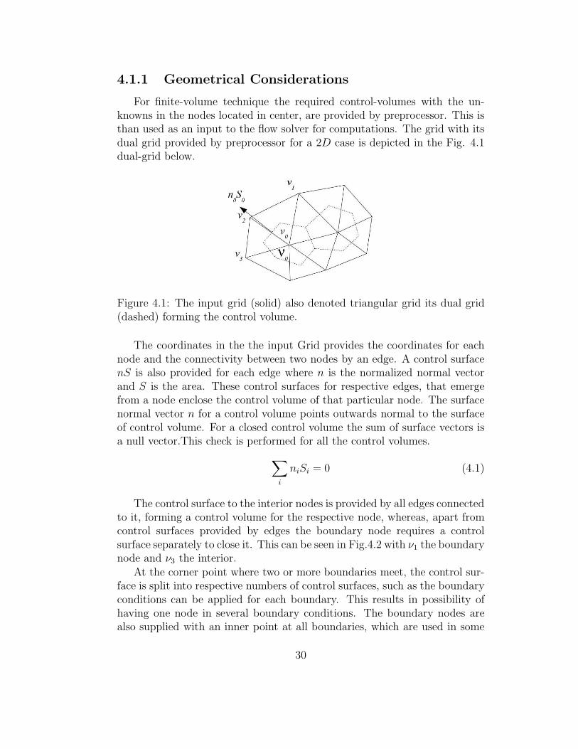
For finite-volume technique the required control-volumes with the un-knowns in the nodes located in center, are provided by preprocessor. This isthan used as an input to the flow solver for computations. The grid with itsdual grid provided by preprocessor for a 2D case is depicted in the Fig. 4.1dual-grid below.
Figure 4.1: The input grid (solid) also denoted triangular grid its dual grid(dashed) forming the control volume.
The coordinates in the the input Grid provides the coordinates for eachnode and the connectivity between two nodes by an edge. A control surfacenS is also provided for each edge where n is the normalized normal vectorand S is the area. These control surfaces for respective edges, that emergefrom a node enclose the control volume of that particular node. The surfacenormal vector n for a control volume points outwards normal to the surfaceof control volume. For a closed control volume the sum of surface vectors isa null vector.This check is performed for all the control volumes.
∑
i
niSi = 0 (4.1)
The control surface to the interior nodes is provided by all edges connectedto it, forming a control volume for the respective node, whereas, apart fromcontrol surfaces provided by edges the boundary node requires a controlsurface separately to close it. This can be seen in Fig.4.2 with ν1 the boundarynode and ν3 the interior.
At the corner point where two or more boundaries meet, the control sur-face is split into respective numbers of control surfaces, such as the boundaryconditions can be applied for each boundary. This results in possibility ofhaving one node in several boundary conditions. The boundary nodes arealso supplied with an inner point at all boundaries, which are used in some
30

Figure 4.2: Control volumes at the inner and the boundary node.
boundary conditions. The inner node is chosen as an end node of the adjacentedge closest to boundary surface.
For 3D cases similar discretization is done. In this case the dual meshconsists of the triangular facets between the centroids of cells, the faces andthe edge. The control volume of a node consists of the faces intersecting themid-point of the edge. At the boundaries additional control faces are addedto form the control volume.
4.2 Boundary Condition
There are two ways to implement the boundary conditions, weak/neumannand strong/dirichlet boundary conditions. Mostly the boundary conditionsare specified as weak boundary conditions, which are imposed by specify-ing the normal derivative of the function on a surface. All the boundarynodes are updated as any interior unknown ensuring the imposed fluxes aremaintained.
∂T
∂n= n.∇T = f(r, t) (4.2)
At some boundaries a strong boundary condition is applied in which theboundary nodes are assigned a constant value which does not change throughout the simulation.
T = f(r, t) (4.3)
One common example of strong boundary condition is the wall boundarycondition where no-slip condition is imposed by setting the wall velocityequal to zero. The boundary conditions applied in the present simulation aredescribed below.
31

4.2.1 Wall Boundary Condition
At wall, there are three types of boundary conditions that can be spec-ified in Edge. Euler condition, Adiabatic and Isothermal, which are chosendepending upon the case. For inviscid flows Euler wall conditions is used,which is a weak condition, since all the variables are unknown and conditionis applied by specifying fluxes, at Euler wall
u1.n = 0 (4.4)
Hence wall fluxes become
f(n) =
0p1nxSp1nySp1nzS0
Similar boundary conditions are used for symmetry conditions.For viscous flows, adiabatic and isothermal boundary conditions are used.
The viscous boundary condition use strong condition on the velocity by set-ting it to zero, implying no-slip condition. The strong boundary condition onvelocity gives better convergence and is sufficiently accurate for fine meshes,as for the weak boundary condition [25].
In case of isothermal wall a weak condition is implied on the constantwall temperature.
For viscous flow most of the boundary conditions used are weak adia-batic, which was also the choice for present simulation. This implies no-slipcondition on velocity. At an adiabatic wall there is no contribution from theviscous terms to the energy equation at a wall since temperature gradientsis zero.
∂T
∂n1
= 0 (4.5)
This means that the boundary flux is zero for both density and energyequation. In addition to the velocity, the turbulent quantities are also im-posed strongly by setting
ν = 0(recommended by SA, 1992) (4.6)
By default it is assumed that the grid at the wall is well resolved to achievey+ ≃ 1 in first layer of node away from the wall unless it is specified to usethe wall functions. If it is specified to use the wall function, a larger value
32
of y+ can be used such that y+ > 30 and first inner nodes are in log-layer,where a finite velocity is specified strongly. In the present case the mesh atwall is well resolved and first layer is such that y+ ≃ 1.
4.2.2 Symmetry Condition
In Edge the symmetry boundary condition are the same as in Euler con-dition, i.e. zero normal velocity as shown in equation 4.4.
4.2.3 Farfield (Weak Characteristic)
In external aerodynamic flows the external boundaries are defined asFarfield, which can handle subsonic and supersonic conditions at inflow andoutflow boundaries. In farfield boundary conditions, characteristics are ei-ther set from free stream quantities for ingoing characteristics or extrapolatedfrom free stream quantities for outgoing characteristics. This depends on thesign of the eigenvalues.
4.3 Running a Computation With Edge
4.3.1 Edge Files
To run a simulation with Edge an input file (*.ainp-file) was preparedfor the SA-DES computation with the freestream settings for Mach num-ber 0.85. Preprocessor was run by providing the input file and *.bedg-filewas obtained. The boundary conditions were specified by running boundcommand and selecting the boundary conditions by feeding the respectivenumber available for each specific condition. Different versions of Edge wereavailable and it was noticed that each version have a specific format for inputfile and also new boundary conditions file (*.aboc-file) needs to be created.Depending upon the size of the computational mesh, multi-processors can bespecified to reduce the simulation time. After the simulations are done theoutput files are merged together by command mergepartitions to obtainone single *.bout-file. For postprocessing the output file was transformedto a format readable by Ensigh by using ffa2engold command. Edge alsoprovides a list of optional post-processing variables, which were not used inpresent simulation. On the other hand the option to record the time-seriesfor unsteady computations was activated. Twenty points were specified byproviding their coordinates and specifying if they are on boundary or interiorin the input file.
33
4.3.2 Grid
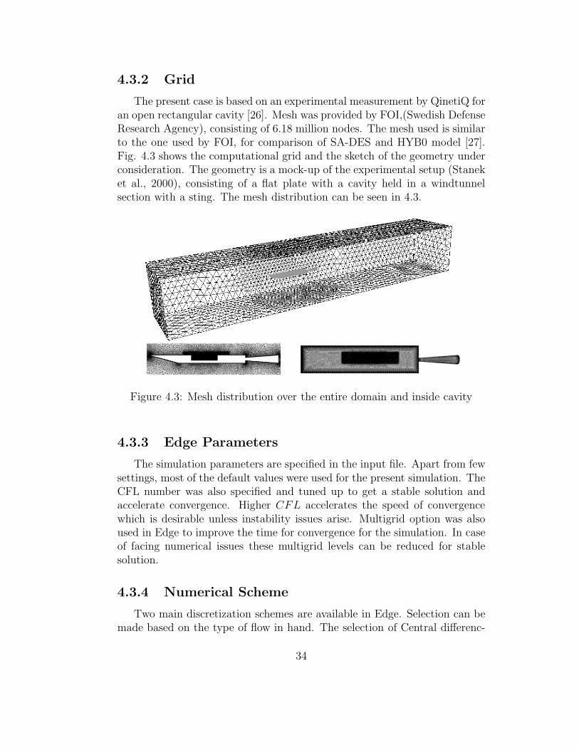
The present case is based on an experimental measurement by QinetiQ foran open rectangular cavity [26]. Mesh was provided by FOI,(Swedish DefenseResearch Agency), consisting of 6.18 million nodes. The mesh used is similarto the one used by FOI, for comparison of SA-DES and HYB0 model [27].Fig. 4.3 shows the computational grid and the sketch of the geometry underconsideration. The geometry is a mock-up of the experimental setup (Staneket al., 2000), consisting of a flat plate with a cavity held in a windtunnelsection with a sting. The mesh distribution can be seen in 4.3.
Figure 4.3: Mesh distribution over the entire domain and inside cavity
4.3.3 Edge Parameters
The simulation parameters are specified in the input file. Apart from fewsettings, most of the default values were used for the present simulation. TheCFL number was also specified and tuned up to get a stable solution andaccelerate convergence. Higher CFL accelerates the speed of convergencewhich is desirable unless instability issues arise. Multigrid option was alsoused in Edge to improve the time for convergence for the simulation. In caseof facing numerical issues these multigrid levels can be reduced for stablesolution.
4.3.4 Numerical Scheme
Two main discretization schemes are available in Edge. Selection can bemade based on the type of flow in hand. The selection of Central differenc-
34
ing scheme over upwind scheme for momentum equation resides in the factof upwind scheme being numerically more dissipative thus might result insmearing up the results and unable to capture interesting flow structures.
4.3.5 Boundary conditions
Correct boundary conditions play an important role in getting the correctflow. Variety of boundary conditions are available and selection is made suchthat the real time conditions are mimiced. At the inlet and outlet pressurefar field boundary conditions are specified. Wall boundary condition wasspecified for the cavity walls. For the test section wall symmetry boundarycondition is used.
4.3.6 Time Integration
The flow at hand is inherently unsteady therefore, time dependent solu-tion is computed by also carrying out discretization in time. Several temporaldiscretization schemes are available. Time-step size and number of inner it-erations are important parameters to achieve reasonable accuracy in eachtime-step and capture the transient flow details.
4.4 The Computational Set-up
The geometric configuration of the cavity used in this project is themock-up of the experiment conducted by the QinetiQ [26]. Experimentwas conducted by mounting the flat plate containing a rectangular cavityinside a 8′ × 8′ transonic wind tunnel. The plate had a length and withof 72 inches and 17 inches respectively. The rectangular cavity has dimen-sions of length L = 20 inches, depth D = 4 inches and width W = 4inches, thus resulting with aspect ratio of L : D : W = 5 : 1 : 1, seeFig.4.4. The experiment was performed under the free stream conditions ofM∞ = 0.85, P∞ = 6.21 × 10⁴Pa, T∞ = 266.53 and Re = 13.47 × 10⁶ permeter.
The computational domain show in Fig. 4.4 consists of a flat plate withlength Lx = 18D and width Ly = 7.5D. At the inlet and outlet Farfieldboundary condition (number31) was specified. The freestream values atthe boundary can be specified here also, if not specified the values from in-put files are used by default. For wind tunnel test section walls symmetryboundary condition (number21) was specified whereas, for cavity and mount-ing boundaries Adiabatic wall boundary condition (number12) was specified.
35

Figure 4.4: The Sketch of the cavity geometry embedded in a plate withLength and width of 72 inches and 17 inches respectively.
Here you can specify wall functions but in this case it wall functions werenot used. The size of the computation demanded use of multi-processorstherefore, it was specified in input file by setting NPART to 48. The CFLnumber was set to 1.25 in the beginning and than later on increased to 1.75since there were no issues with the instability in the simulation. Four lev-els of multigrid were selected with a default settings of W − cycle. TheSpalart-Allmaras model is selected in Edge by setting ITURB = 3, andTURB MOD NAME =′ Spalart − AllmarasDESmodel′. For the DESthe central difference scheme was used with second order implicit time inte-gration. Central Differencing scheme was also used for the turbulent trans-port equations. Pressure far field conditions were applied on the inflow andoutflow boundaries with freestream conditions of Mach number M = 0.85,temperature T = 266.528 K, pressure P = 62096 Pa and eddy vis-cosity ratio of µt/µ0 = 10. The five cavity walls and the geometry wallscontaining the cavity are specified as adiabatic wall boundary with no-slipcondition. The ideal boundary condition for the outer (wind tunnel sec-tion) walls would have been non-reflective boundary condition. Whereas,the best available boundary condition was symmetry which was applied.The DES computation was initialized with the Reynolds-averaged Navier-Stokes (RANS) solution. A time-step size of 2 × 10⁻⁵ seconds was selectedon the basis of study made by Larcheveque et al. (2001) [4] suggesting thata time-step around ∆t = 2 × 10⁻⁵ or smaller should be sufficient for thisparticular test case. A maximum of 70 inner iterations were carried out for
36

each time-step to ensure adequate convergence. The computations were runfor a total of 13, 000 time-steps or 0.26 seconds real time. The time averagingwas started after first 2000 iterations, ensuring the flow is developed insidethe cavity.
37

38
Chapter 5
Results and Discussion
5.1 2D Results
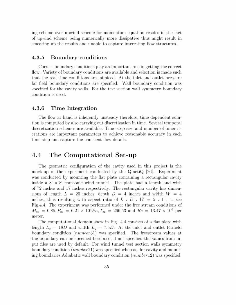
The study of the flow over a cavity was started with 2D computations tounderstand the basic flow physics and compare the effect of different turbu-lence models. The turbulence models used for the computations include theSA, EARSM, SST k-omega and Wilcox turbulence models.
Figure 5.1: Computational domain used for 2D simulations
5.1.1 Computational setup
The computational domain used for carrying out 2D simulations is shownin Fig. 5.1. The domain size in x-direction and y-direction are Lx = 18Dand Ly = 7.5D respectively. The leading edge of the cavity is located at a
39
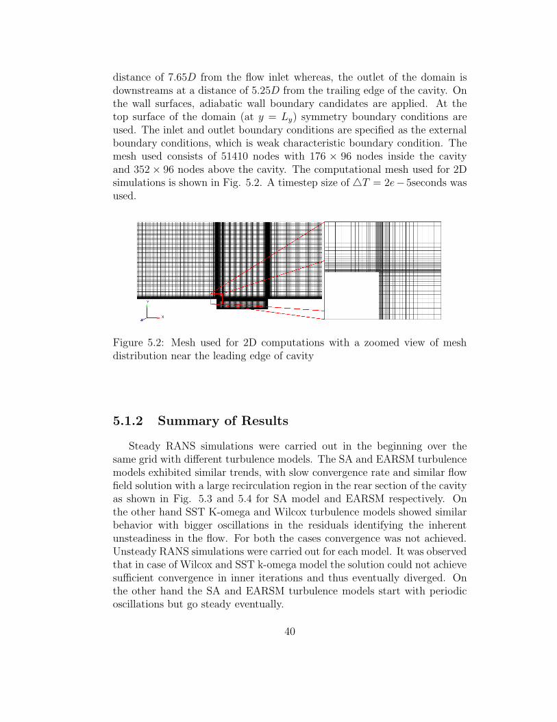
distance of 7.65D from the flow inlet whereas, the outlet of the domain isdownstreams at a distance of 5.25D from the trailing edge of the cavity. Onthe wall surfaces, adiabatic wall boundary candidates are applied. At thetop surface of the domain (at y = Ly) symmetry boundary conditions areused. The inlet and outlet boundary conditions are specified as the externalboundary conditions, which is weak characteristic boundary condition. Themesh used consists of 51410 nodes with 176 × 96 nodes inside the cavityand 352 × 96 nodes above the cavity. The computational mesh used for 2Dsimulations is shown in Fig. 5.2. A timestep size of T = 2e−5seconds wasused.
Figure 5.2: Mesh used for 2D computations with a zoomed view of meshdistribution near the leading edge of cavity
5.1.2 Summary of Results
Steady RANS simulations were carried out in the beginning over thesame grid with different turbulence models. The SA and EARSM turbulencemodels exhibited similar trends, with slow convergence rate and similar flowfield solution with a large recirculation region in the rear section of the cavityas shown in Fig. 5.3 and 5.4 for SA model and EARSM respectively. Onthe other hand SST K-omega and Wilcox turbulence models showed similarbehavior with bigger oscillations in the residuals identifying the inherentunsteadiness in the flow. For both the cases convergence was not achieved.Unsteady RANS simulations were carried out for each model. It was observedthat in case of Wilcox and SST k-omega model the solution could not achievesufficient convergence in inner iterations and thus eventually diverged. Onthe other hand the SA and EARSM turbulence models start with periodicoscillations but go steady eventually.
40

Figure 5.3: Streamlines with mach number contours on the central sectiony/W = 0 for SA model
Figure 5.4: Streamlines with mach number contours on the central sectiony/W = 0 for EARSM
5.2 3D Results
5.2.1 Mean Flow Comparison
The mean flow features were compared with the available resolved LESdata by Larcheveque et al.,(2004) [28]. To begin with mean longitudinal andvertical velocity were compared at specific locations (x/D = 0, 0.1, 0.2, 0.3,0.4, 0.5, 0.6, 0.7, 0.8, 0.9, 1) on mid-plane of cavity (y = 0.0254m). From Fig.5.5 it can be seen that the DES profile matches fairly well with the LES datawith some discrepancies in shearlayer close to the leading edge of the cavity,but gets better agreement with the reference data further downstreams. Thiscan be because of the incoming boundary layer is not well resolved since weuse RANS in the region close to wall and switch to LES further away fromthe wall. Another cause for the difference at the leading edge might be themodeled stream depletion, which is caused by mesh size and the LES regionfalls in the boundary layer.
In Fig. 5.6, comparison is shown between the DES and reference LES
41

Figure 5.5: Mean streamwise velocity (U) profile on the central sectiony/W = 0, in comparison with LES data [28] at specific locations over thecavity length
vertical velocity profiles, showing an obvious difference at some locations.The negative part of the profile is the indication of the deflection of theshear layer towards the cavity floor. Close to the leading edge of the cavityat x/L = 0.1 the vertical velocity W is in good comparison with the LESprofiles. At locations x/L = 0.2 and 0.3 there is a slight over prediction in thepositive part of the profile and further downstreams at x/L = 0.4, 0.5 and 0.6the W component of the velocity is under predicted showing that the strengthof the large recirculation region is under predicted as compared to LES. Onereason for a poor match can be the mesh resolution inside the cavity, wheresome part of the flow gets separated from the shear layer and give rise toa recirculation region. Close to the trailing edge of the cavity the verticalvelocity and longitudinal velocity profiles matches nicely identifying that thesmaller recirculation region is well captured. The shear layer predicted byDES is comparable with the LES, as the flow approaches the aft wall. Thisis verified by a good match between the vertical velocity (negative part ofthe) profile at all stations.
As discussed above the grid resolution seems not enough to resolve theshear layer, as also can be noticed in Fig. 5.7 where the shear stresses areplotted in comparison with the reference LES data, note that the last profileis at x/L = 0.995. Here we notice that the shear layer is predicted withlarge discrepancies specially in the first half of the cavity and also somediscrepancies are observed in the recirculation region.A much better flowstructure can be achieved by refining the mesh in cavity in general and shearlayer in particular. Also the regions downstream where there are complexflow structures in terms of changing direction more rapidly. More specificallythe kink in profile at x/L = 0.7 is the location of interaction between the bigand small recirculation region.
42
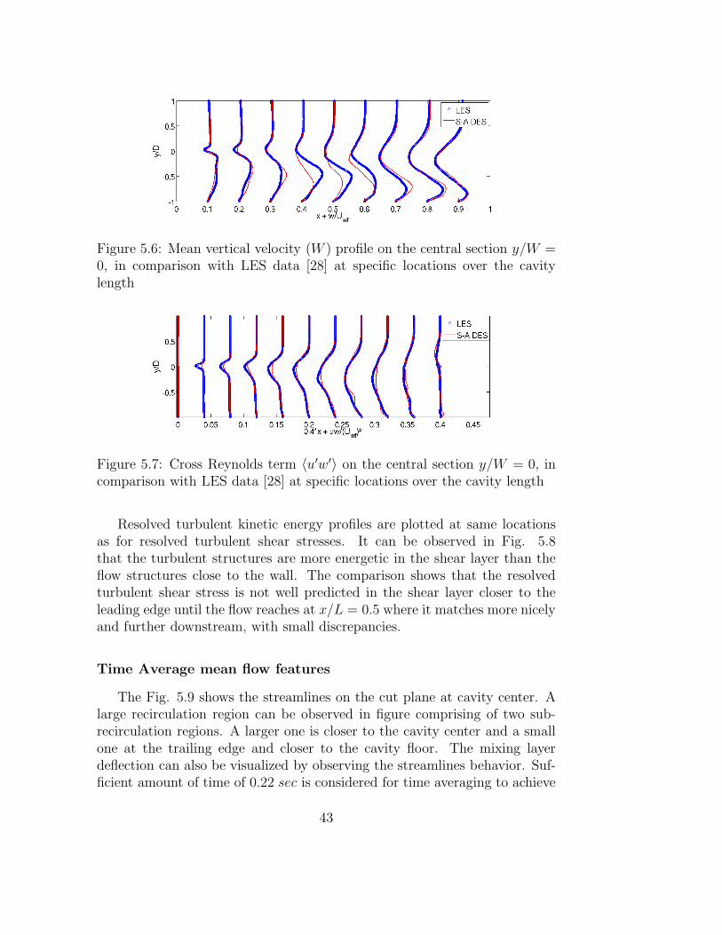
Figure 5.6: Mean vertical velocity (W ) profile on the central section y/W =0, in comparison with LES data [28] at specific locations over the cavitylength
Figure 5.7: Cross Reynolds term 〈u′w′〉 on the central section y/W = 0, incomparison with LES data [28] at specific locations over the cavity length
Resolved turbulent kinetic energy profiles are plotted at same locationsas for resolved turbulent shear stresses. It can be observed in Fig. 5.8that the turbulent structures are more energetic in the shear layer than theflow structures close to the wall. The comparison shows that the resolvedturbulent shear stress is not well predicted in the shear layer closer to theleading edge until the flow reaches at x/L = 0.5 where it matches more nicelyand further downstream, with small discrepancies.
Time Average mean flow features
The Fig. 5.9 shows the streamlines on the cut plane at cavity center. Alarge recirculation region can be observed in figure comprising of two sub-recirculation regions. A larger one is closer to the cavity center and a smallone at the trailing edge and closer to the cavity floor. The mixing layerdeflection can also be visualized by observing the streamlines behavior. Suf-ficient amount of time of 0.22 sec is considered for time averaging to achieve
43
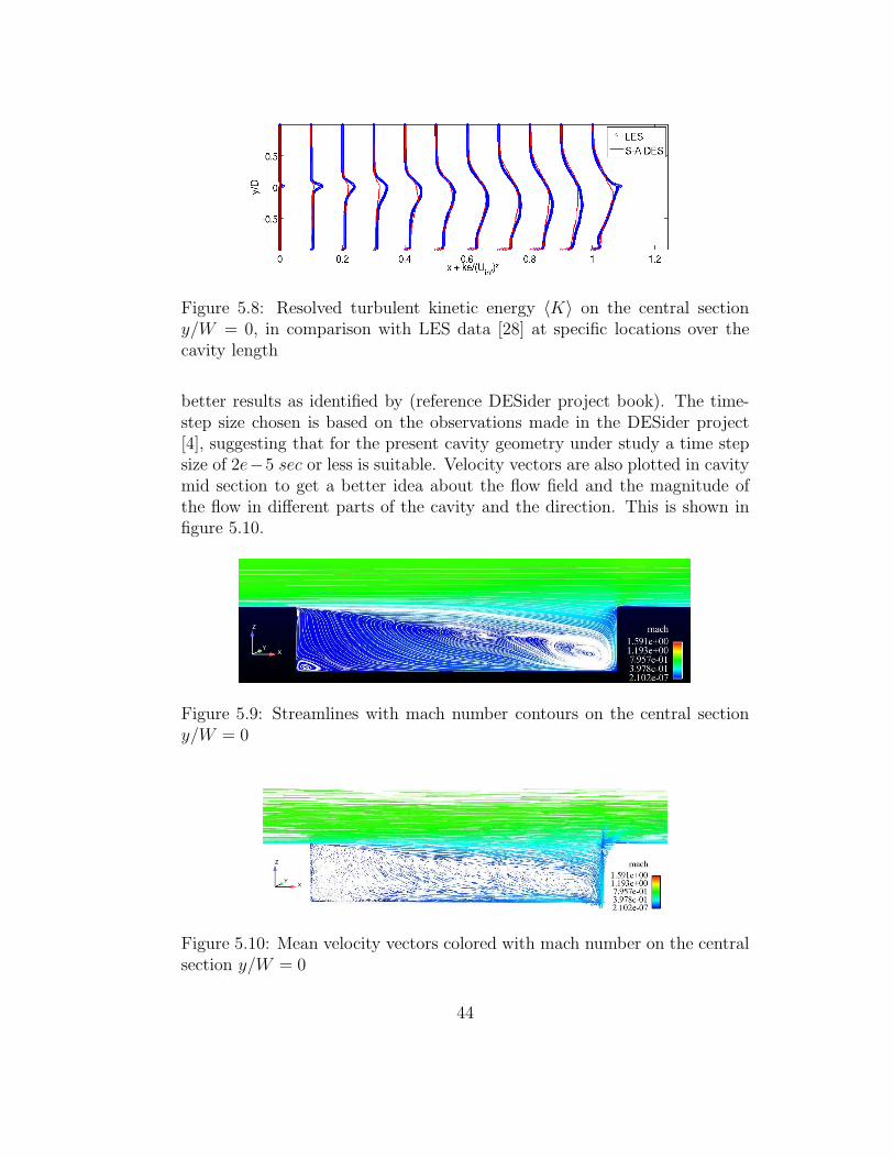
Figure 5.8: Resolved turbulent kinetic energy 〈K〉 on the central sectiony/W = 0, in comparison with LES data [28] at specific locations over thecavity length
better results as identified by (reference DESider project book). The time-step size chosen is based on the observations made in the DESider project[4], suggesting that for the present cavity geometry under study a time stepsize of 2e−5 sec or less is suitable. Velocity vectors are also plotted in cavitymid section to get a better idea about the flow field and the magnitude ofthe flow in different parts of the cavity and the direction. This is shown infigure 5.10.
Figure 5.9: Streamlines with mach number contours on the central sectiony/W = 0
Figure 5.10: Mean velocity vectors colored with mach number on the centralsection y/W = 0
44
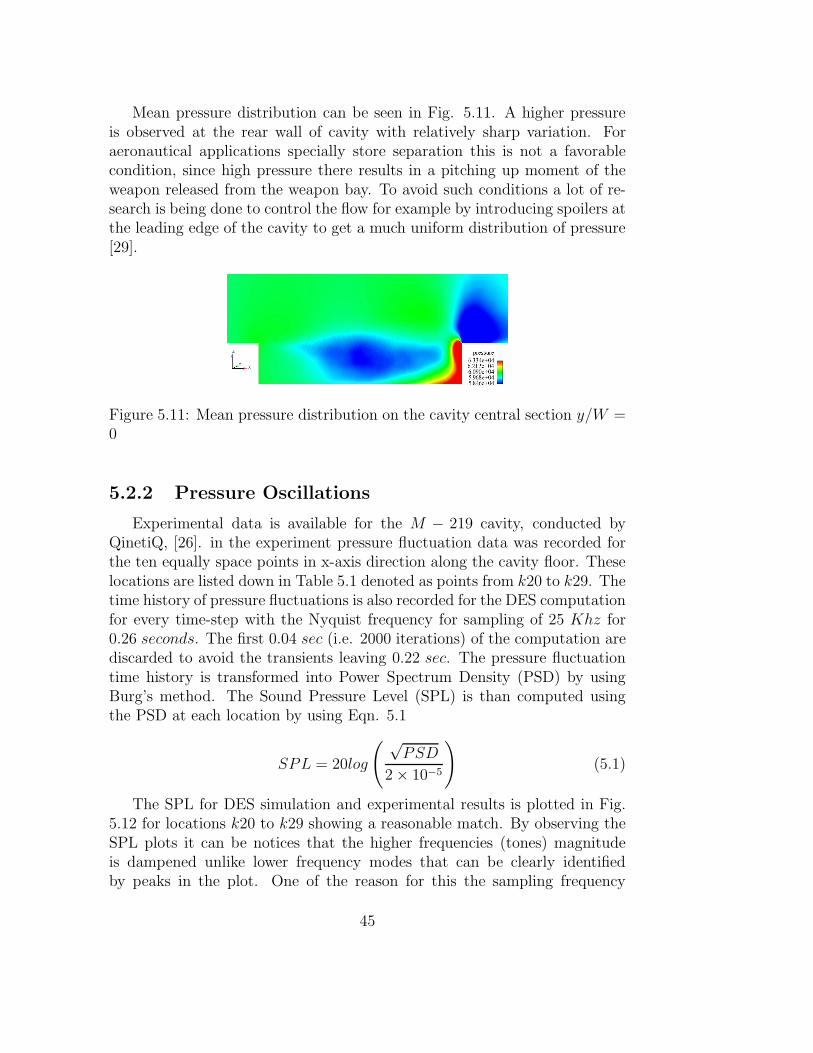
Mean pressure distribution can be seen in Fig. 5.11. A higher pressureis observed at the rear wall of cavity with relatively sharp variation. Foraeronautical applications specially store separation this is not a favorablecondition, since high pressure there results in a pitching up moment of theweapon released from the weapon bay. To avoid such conditions a lot of re-search is being done to control the flow for example by introducing spoilers atthe leading edge of the cavity to get a much uniform distribution of pressure[29].
Figure 5.11: Mean pressure distribution on the cavity central section y/W =0
5.2.2 Pressure Oscillations
Experimental data is available for the M − 219 cavity, conducted byQinetiQ, [26]. in the experiment pressure fluctuation data was recorded forthe ten equally space points in x-axis direction along the cavity floor. Theselocations are listed down in Table 5.1 denoted as points from k20 to k29. Thetime history of pressure fluctuations is also recorded for the DES computationfor every time-step with the Nyquist frequency for sampling of 25 Khz for0.26 seconds. The first 0.04 sec (i.e. 2000 iterations) of the computation arediscarded to avoid the transients leaving 0.22 sec. The pressure fluctuationtime history is transformed into Power Spectrum Density (PSD) by usingBurg’s method. The Sound Pressure Level (SPL) is than computed usingthe PSD at each location by using Eqn. 5.1
SPL = 20log
( √PSD
2 × 10⁻⁵
)(5.1)
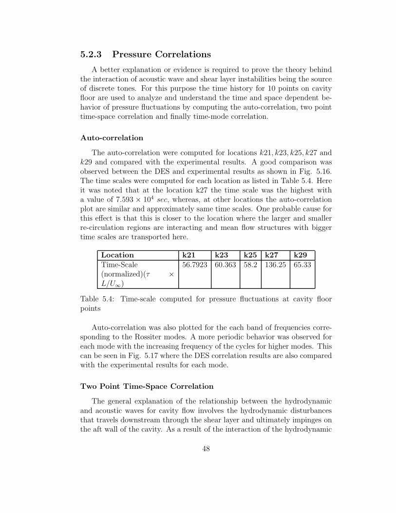
The SPL for DES simulation and experimental results is plotted in Fig.5.12 for locations k20 to k29 showing a reasonable match. By observing theSPL plots it can be notices that the higher frequencies (tones) magnitudeis dampened unlike lower frequency modes that can be clearly identifiedby peaks in the plot. One of the reason for this the sampling frequency
45

at which the pressure fluctuations are recorded, apart from that it mustbe noted that the smaller structures have shorter time scales. Therefore,in case of using a larger timestep may defile these structures or not evencapture them at all. This might affect the results for higher frequencies sincethe fast evolving structures are not well resolved. Besides these constraints,unphysical numerical diffusion might also result in dampened SPL magnitudeat these higher frequencies.
Kultie x(inches) y(inches) z(inches)k20 1.0 0.0 -4.0k21 3.0 0.0 -4.0k22 5.0 0.0 -4.0k23 7.0 0.0 -4.0k24 9.0 0.0 -4.0k25 11.0 0.0 -4.0k26 13.0 0.0 -4.0k27 15.0 0.0 -4.0k28 17.0 0.0 -4.0k29 19.0 0.0 -4.0
Table 5.1: Specified locations on cavity floor from aft wall for pressure mea-surement
The peaks in the SPL plots are corresponding to a discrete frequencyidentifying a particular mode. First four modes are identified clearly bynumerical results at k20 and k21. As discussed above the fourth mode cor-responding to higher frequency, the SPL-magnitude is not very well resolvedby the SA-DES model. Whereas, the second and third mode are clearly cap-tured in almost all the locations. From Fig. 5.12 it can be observed that theSPL magnitude for the first mode is the least well predicted with under pre-diction of approximately 2 − 7 dB. On the other hand the second and thirdmodes are well predicted with an under prediction ranging from less than1-3 dB except for the third mode being slightly over predicted at k21. Thefourth mode is over and under predicted in a range of ±2 dB. The resonancefrequencies for each mode are captured fairly well with a maximum differenceof 29 Hz for fourth mode. The predicted frequencies for each mode are com-pare with the experimental data and Rossiter modes frequencies in Table 5.2.For the SA-DES results also a percentage difference with the experimentalresults is listed corresponding to each mode.
Overall Sound Pressure Level (OASPL) is also plotted on the cavity floorand compared with the experimental results available. From Fig. 5.13 it
46

Modes Frequency(Hz)
Mode 1 Mode 2 Mode 3 Mode 4
QinetiQ Experiment 135 350 590 820Rossiter’s Formula 148 357 566 775SA-DES 133 376 595 849Percentage differencebetween SA-DES andExperiment
1.48 7.43 0.85 3.53
Table 5.2: Comparison of frequencies for four tonal modes
can be seen that the OASPL computed by SA-DES compares well with theexperimental results specially at the rear part of the cavity. OASPL is slightlyover predicted with the maximum difference of magnitude less than 1.5 dB.It can be no tied that the general trend or the shape of the plot is similarto the experimental results, showing that the flow behavior over the cavityfloor in terms of pressure fluctuations is similar.
Band Integrated Sound Pressure (BISPL) was also computed by filteringbands of frequencies corresponding to each Rossiter mode and than trans-forming it back to time domain and integrating for OASPL for each band.The frequency band ranges for each Rossiter mode have a band width of100 Hz and spread over a range of frequencies such as to capture the peaksfor both experimental and DES computations. These frequency ranges canbe seen in Table 5.3. The computational results for BISPL for each modeare plotted and compared with the experimental results in Fig. 5.14. Here itcan be seen that the modal shapes for each mode are well captured but withthe over-prediction of magnitude by approximately 20 dB for each mode.This difference in magnitude is far more than the error observed by LES forthe same geometry [28]. Same procedure was repeated at the cutplane aty/W = 0, for which a time-history was available for all the nodes after every5 timesteps which means after every 1e − 4 sec. The mode shapes for eachmode were plotted over the cutplane to identify the regions where each modewas dominant, as seen in Fig. 5.15.
Rossiter Mode 1 2 3 4Lower limit (Hz) 100 300 550 800Upper limit (Hz) 200 400 650 900
Table 5.3: Upper and lower limits of frequency bands for each Rossiter mode
47
5.2.3 Pressure Correlations
A better explanation or evidence is required to prove the theory behindthe interaction of acoustic wave and shear layer instabilities being the sourceof discrete tones. For this purpose the time history for 10 points on cavityfloor are used to analyze and understand the time and space dependent be-havior of pressure fluctuations by computing the auto-correlation, two pointtime-space correlation and finally time-mode correlation.
Auto-correlation
The auto-correlation were computed for locations k21, k23, k25, k27 andk29 and compared with the experimental results. A good comparison wasobserved between the DES and experimental results as shown in Fig. 5.16.The time scales were computed for each location as listed in Table 5.4. Hereit was noted that at the location k27 the time scale was the highest witha value of 7.593 × 10⁴ sec, whereas, at other locations the auto-correlationplot are similar and approximately same time scales. One probable cause forthis effect is that this is closer to the location where the larger and smallerre-circulation regions are interacting and mean flow structures with biggertime scales are transported here.
Location k21 k23 k25 k27 k29Time-Scale(normalized)(τ ×L/U∞)
56.7923 60.363 58.2 136.25 65.33
Table 5.4: Time-scale computed for pressure fluctuations at cavity floorpoints
Auto-correlation was also plotted for the each band of frequencies corre-sponding to the Rossiter modes. A more periodic behavior was observed foreach mode with the increasing frequency of the cycles for higher modes. Thiscan be seen in Fig. 5.17 where the DES correlation results are also comparedwith the experimental results for each mode.
Two Point Time-Space Correlation
The general explanation of the relationship between the hydrodynamicand acoustic waves for cavity flow involves the hydrodynamic disturbancesthat travels downstream through the shear layer and ultimately impinges onthe aft wall of the cavity. As a result of the interaction of the hydrodynamic
48

wave and cavity aft wall, acoustic waves are generated that propagates up-streams and eventually interacts with the shear layer at the cavity leadingedge. Discrete tones (Rossiter modes) are created when this interaction re-sults in resonance of either acoustic or hydrodynamic wave. The pressuremeasured on the cavity wall consists of disturbances of various wavelengthstraveling in different directions inside the cavity. Therefore, it suggests thatthese pressures on cavity surface are highly correlated in specific wavelengthbands. Now it is important to somehow show that these disturbances arepropagating in the cavity at physically significant speeds. Therefore, twopoint time-space correlation is carried out and presented in Fig. 5.18. Forthis purpose the cavity floor points are used and two point time-space corre-lation are computed by keeping k29 as source and moving along k21, k23, k25and k27 and comparison is also made with the correlation plots for the ex-perimental data.
Here it must be noted that each set of correlation exhibit a cyclic behaviorby showing a maximum peak followed by a periodic structure showing someresonating effects. It can be noted from Fig. 5.18 that the correlation plotsdoes not indicate a decaying pattern of one frequency thus indicating thepresence of multiple repetitive signals. Furthermore, in Fig. 5.19 the firstpeaks are marked with star showing the time lag between each peak, whichindicates the time taken by an event when it is sensed at the other location.This is an indication of propagation of disturbances inside the cavity.
Time-Mode Correlation
The power spectrum identified the presence of four Rossiter modes. Tocome up with a way to show which mode is more dominant in terms of beingmore correlated and therefore, causing more interaction with the cavity flowstructures ( The entire signal). For this purpose the frequency bands werefiltered out from the entire spectrum and transformed back from frequencydomain to time domain by taking Inverse Fast Fourier Transform (ifft) inmatlab. The time-mode correlation was computed between each mode andentire signal for cavity floor points. It was observed that the first mode wasmore correlated as compared to the rest of the modes. This was expectedsince the hydrodynamic waves are not accompanied with high frequencies.Therefore, the first mode being low frequency had a better correlation. Asthe frequency is increased the correlation coefficient magnitude is reduced asshown in Fig. 5.20.
49
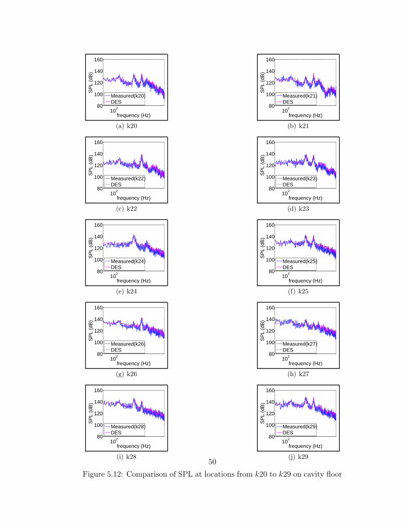
10280
100
120
140
160
frequency (Hz)
SP
L (d
B)
Measured(k20)DES
(a) k20
10280
100
120
140
160
frequency (Hz)
SP
L (d
B)
Measured(k21)DES
(b) k21
10280
100
120
140
160
frequency (Hz)
SP
L (d
B)
Measured(k22)DES
(c) k22
10280
100
120
140
160
frequency (Hz)
SP
L (d
B)
Measured(k23)DES
(d) k23
10280
100
120
140
160
frequency (Hz)
SP
L (d
B)
Measured(k24)DES
(e) k24
10280
100
120
140
160
frequency (Hz)
SP
L (d
B)
Measured(k25)DES
(f) k25
10280
100
120
140
160
frequency (Hz)
SP
L (d
B)
Measured(k26)DES
(g) k26
10280
100
120
140
160
frequency (Hz)
SP
L (d
B)
Measured(k27)DES
(h) k27
10280
100
120
140
160
frequency (Hz)
SP
L (d
B)
Measured(k28)DES
(i) k28
10280
100
120
140
160
frequency (Hz)
SP
L (d
B)
Measured(k29)DES
(j) k29
Figure 5.12: Comparison of SPL at locations from k20 to k29 on cavity floor
50
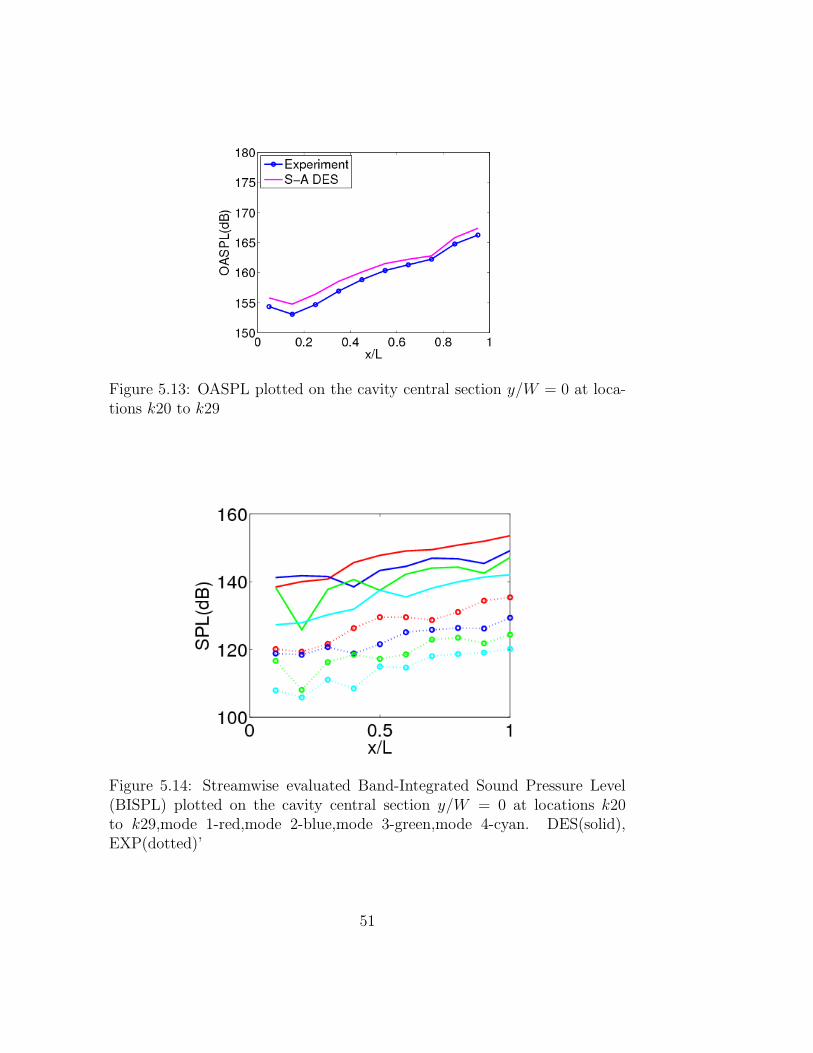
Figure 5.13: OASPL plotted on the cavity central section y/W = 0 at loca-tions k20 to k29
Figure 5.14: Streamwise evaluated Band-Integrated Sound Pressure Level(BISPL) plotted on the cavity central section y/W = 0 at locations k20to k29,mode 1-red,mode 2-blue,mode 3-green,mode 4-cyan. DES(solid),EXP(dotted)’
51
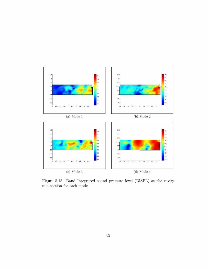
(a) Mode 1 (b) Mode 2
(c) Mode 3 (d) Mode 4
Figure 5.15: Band Integrated sound pressure level (BISPL) at the cavitymid-section for each mode
52
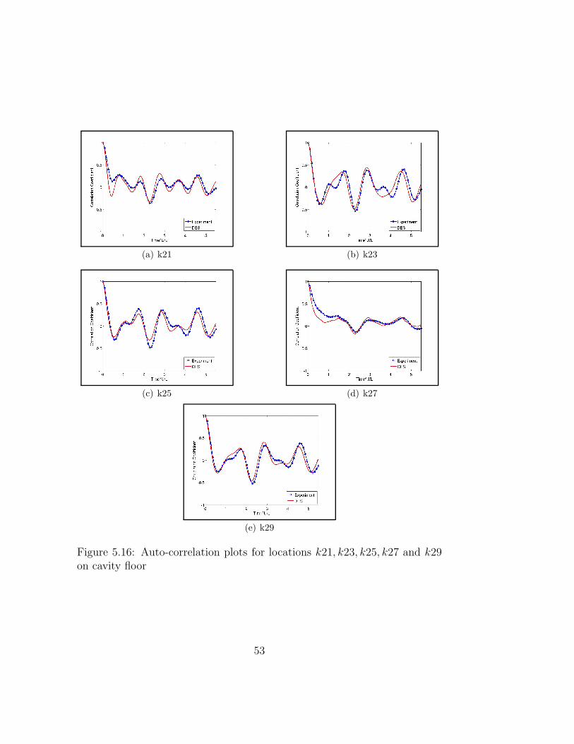
(a) k21 (b) k23
(c) k25 (d) k27
(e) k29
Figure 5.16: Auto-correlation plots for locations k21, k23, k25, k27 and k29on cavity floor
53

(a) Mode 1 (b) Mode 2
(c) Mode 3 (d) Mode 4
Figure 5.17: Auto-correlation plots for frequency band corresponding toRossiter modes at locations k29 on cavity floor
54
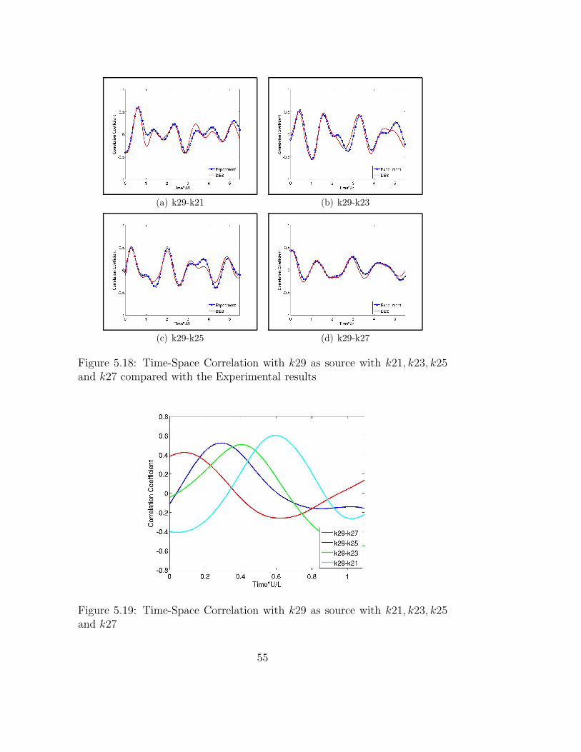
(a) k29-k21 (b) k29-k23
(c) k29-k25 (d) k29-k27
Figure 5.18: Time-Space Correlation with k29 as source with k21, k23, k25and k27 compared with the Experimental results
Figure 5.19: Time-Space Correlation with k29 as source with k21, k23, k25and k27
55
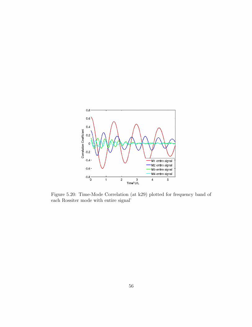
Figure 5.20: Time-Mode Correlation (at k29) plotted for frequency band ofeach Rossiter mode with entire signal’
56
Chapter 6
Conclusion and Outlook
6.1 Conclusion and Outlook
The SA-DES turbulence model is used to simulate a high Reynolds num-ber flow over a three-dimensional cavity. The computational results are val-idated by comparison with the available experimental and LES data. Thepredicted pressure fluctuations are compare with the experimental data avail-able. Whereas, time-averaged mean flow features are compared with theavailable LES results. In general the instantaneous as well as the mean flowfeatures were reasonably well resolved by SA-DES.
The pressure fluctuations were analyzed by computing sound pressurelevel (SPL) where the four tonal modes were also revealed as peaks in thespectrum. The frequencies corresponding to these modes were independentof the location over the cavity length. The second and third mode were moredominant as they were clearly captured at almost every location. The DEScomputation did not produce the fourth mode well as at some locations peakwas smeared. The overall sound pressure level calculated from DES gives areasonable agreement with the experiment, more specifically in the secondhalf of the cavity. The mean flow features observed in DES computationagreed well with the benchmark LES findings. However in the recirculationregion there are some discrepancies clearly visible from the mean verticalvelocity plots. The incoming boundary layer is not very well resolved bySA-DES as compared to the LES, this is indicated in the mean streamwisevelocity profile close to the leading edge of the cavity.
A cyclic behavior of the time-space correlation without decaying in mag-nitude of correlation coefficient shows that multiple wavelength waves aretraveling in different directions in the cavity. The first mode is more corre-lated to the entire signal as compared to the higher frequency modes. The
57

correlation magnitude reduces as we move to higher frequency modes as in-dicated by the time-mode correlation plots.
The results seem motivating specially the correlation analysis. In futureefforts can be made to store the data for entire domain at each time step andthe pressure correlation analysis can be carried out to get a more accurateinsight into the shear layer. Better filtering techniques can be applied tofilter out the signal noise while studying frequency bands for each mode.
58

Bibliography
[1] A. Roshko. Some measurements of flow in a rectangulat cutout. Tech-nical note - 3488, National Advisory Committee for Aeronautics, Wash-ington, USA, 1955.
[2] T. Colonius C. W. Rowley and A. J. Basu. On self-sustained oscillationsin two-dimentional compressible flow over rectangular cavities. J. FluidMech., 455:315–346, 2002.
[3] J. E. Rossiter. Wind-tunnel experiments on the flow over rectangularcavities at subsonic and transoni speeds. Reports and memoranda 3438,Aeronautical Research Council, 1964.
[4] S.-H. Peng. Application - Test Cases: M219 cavity flow. In DESider - AEuropean Effort on Hybrid RANS-LES Modelling, volume 103 of Noteson Numerical Fluid Mechanics and Multidisciplinary Design, pages 270–285. Springer Verlag, 2007.
[5] N. Toy P. J. Dislmile and E. Savory. Effect of planform aspect ratioon flow oscillations in rectangular cavities. Trans. ASME: J of FluidsEngineering., 122:32–38, 2000.
[6] K. K. Ahuja and J. Mendoza. Effects of cavity dimensions, boundarylayer, and temperature on cavity noise with emhasis on benchmark datato validate computational aeroacoustic codes. Contractor report 4653,NASA, 1995.
[7] S. T. Bjorge. Flow around an object projected from a cavity into a su-personic freestream. Msc thesis, Department of the Air Force Air Uni-versity, Air Force Institute of Technology, Wright-Patterson Air ForceBase, Ohio, USA, 2004.
[8] D. M. Bortz et al. Reduced order modelling in control of open cavityacoustics. Technical report a820454, Center for Research in Scientific
59
Computation, North Carolina State University, Raleigh, North Carolina,USA, 2000.
[9] S.Garg M. Kegerise, E. Spina and L. Cattafesta. Mode-switching andnonlinear effects in compressible flow over a cavity. Physics of Fluids,16(3):678–687, 2004.
[10] P. J. W. Block. Noise response of cavities of varying dimensions atsubsonic speeds. Technical note d-8351, NASA, 1976.
[11] M. B. Tracy and E. B. Plentovich. Characterization of cavity flow fieldsusing pressure data obtained in the langley 0.3-meter transonic cryo-genic tunnel. Technical memorandum 4436, NASA, Langley ResearchCenter,Hampton, Virginia, USA, 2004.
[12] A. J. Basu T. Colonius and C. W. Rowley. Numerical investigationof the flow past a cavity. In AIAA Paper 99-1912, 5th AIAA/CEASAeroacoustics Conference, May, Bellevue, Washington, USA, 1999.
[13] L. L. Shaw R. S. Gates, C. Butler and R.E. Dix. Aeroacoustic effectsof body blockage in cavity flow. In AIAA Paper 87-2667, 11th AIAAAeroacoustics Conference, 19-21 Oct, Sunnyvale, California, USA, 1987.
[14] V. Sarohia and P.E. Massier. Control of cavity noise. Journal of Aircraft,14:833–837, 1977.
[15] D. Rockwell and E. Naudascher. Review - self-sustaining engineeringapplications of computational fluid mechanicsoscillations of flow pastcavities. Journal of Fluids Engineering, 100:152–165, 1978.
[16] P.R. Spalart, W.-H. Jou, M. Strelets, and S.R. Allmaras. Comments onthe feasability of LES for wings and on a hybrid RANS/LES approach.In C. Liu and Z. Liu, editors, Advances in LES/DNS, First Int. conf.on DNS/LES, Louisiana Tech University, 1997. Greyden Press.
[17] P. R. Spalart and S. R. Allmaras. A one-equation turbulence model foraerodynamic flow. Larecherche aerospatiale, 1:5–21, 1994.
[18] C. David Wilcox. Reassessment of the scale-determining equation foradvanced turbulence model. AIAA Journal, 26:1299–1310, 1988.
[19] F. R. Menter. Two-equation eddy-viscosity turbulence models for engi-neering applications. AIAA Journal, 32:1598–1605, 1994.
60
[20] Stefan Wallin and Arne V. Johansson. An explicit algebraic reynoldsstress model for incompressible and compressible turbulent flows. Jour-nal of Fluid Mechanics, 403:89 – 132, 2000.
[21] Stefan Wallin and Arne V. Johansson. Modelling streamline curvatureeffects in explicit algebraic reynolds stress turbulence models. Interna-tional Journal of Heat and Fluid Flow, 23:721 – 730, 2002.
[22] A. Hellsten. New advanced k-omega turbulence model for high-lift aero-dynamics. AIAA Journal, 43:1857 – 1869, 2005.
[23] FOI. Edge user guide. User manual, foi dnr 03-2879, Defense and Secu-rity, Systems and Technology, FOI, Swedish Defense Research Agency,Stockholm, Sweden, 2007.
[24] FOI. Edge theoratical formulation. User manual, foi dnr 03-2879, De-fense and Security, Systems and Technology, FOI, Swedish Defense Re-search Agency, Stockholm, Sweden, 2007.
[25] Q. Abbas and J. Nordstrm. Weak versus. strong no-slip boundary condi-tions for the navier stokes equations. Engineering Applications of Com-putational Fluid Mechanics, 4:29–38, 2010.
[26] M. Henshaw and J. de Charentenay. In verification and validation datafor computational unsteady aerodynamics. Technical report rto-tr-26,ac/323(avt)tp/19, QinetiQ, British Aerospace (Operations) Ltd., Mili-tary Aircraft and Aerostructures Skillings Lane, Brough, East Riding ofYorkshire, HU151EQ U.K., 2002.
[27] S. H. Peng and S. Leicher. Des and hybrid rans-les modelling of unsteadypressure oscillations and flow features in a rectangular cavity. S. -H.Peng., W. Haase, Advances in Hybrid RANS-LES Modelling. Notes onNumerical Fluid Mechanics and Multidisciplinary Design, 97:132–141,2008.
[28] T.-H. Le L. Larcheveque, P. Sagaut and P-Comte. Large-eddy simula-tion of a compressible flow in a three-dimentional open cavity at highreynolds number. Journal of Fluid Mechanics, 516:265–301, 2004.
[29] M. Mallet V-Levasseur, P. Sagaut and F. Chalot. Unstructured largeeddy simulation of the passive control of the flow in a weapon bay.Journal of Fluids and Structures, 24:1204–1215, 2008.
61