Thesis 4-26-09

8/3/2019 Thesis 4-26-09

http://slidepdf.com/reader/full/thesis-4-26-09 1/62

Combinatorics of Periodic Points of Interval Maps

Tyler London

Department of Mathematics

College of Liberal Arts and SciencesTufts University

Senior Honors Thesis

· 2009 ·

8/3/2019 Thesis 4-26-09


Abstract

In 1964, Sharkovsky showed that there is a linear ordering ≤s of the natural numberssuch that m ≤s n if every continuous interval map having an n-periodic point has anm-periodic point. This idea is generalized to get a partial ordering of cyclic permutationscalled the forcing relation by taking into consideration the pattern of the periodic orbit.We show that forcing can be reduced to the study of certain canonical piecewise linear

maps. Combinatorial algorithms of Baldwin and Coven et. al. that decide forcing arepresented, as well as a diagram of the forcing relation on over 190 cycles of length up to8. The global structure of forcing is described by considering flips of cycles and unimodal cycles. It is shown that the forcing relation restricted to unimodal cycles is a total ordering,and this relation is diagrammed on 115 unimodal cycles. The local structure of forcingis also explored by studying doublings and extensions. A new combinatorial proof of atheorem describing the structure of doublings in the forcing order is given. Forcing-minimalproperties are examined by considering primary and simple cycles. Finally, using theresults proven about the forcing relation, we derive Sharkovsky’s theorem as a consequenceof the forcing theorem.

Key words and phrases. Interval maps, periodic orbit, Markov graph, Sharkovsky’s theo-rem, cycle, forcing, doubling, block structure, extension, primary cycle, simple cycle.

8/3/2019 Thesis 4-26-09


Contents

Acknowledgments iii

0 Introduction 1

1 Background 31.1 Cyclic Permutations . . . . . . . . . . . . . . . . . . . . . . . . . . . . . . . 31.2 Continuous Maps of the Interval . . . . . . . . . . . . . . . . . . . . . . . . 51.3 The Theorem of Sharkovsky . . . . . . . . . . . . . . . . . . . . . . . . . . . 8

2 The Forcing Relation on Cycles 11

2.1 The Combinatorial Data in a Periodic Orbit . . . . . . . . . . . . . . . . . . 112.2 The Forcing Theorem . . . . . . . . . . . . . . . . . . . . . . . . . . . . . . 13

3 A Computational Digression 20

3.1 Description of the Algorithm of Baldwin . . . . . . . . . . . . . . . . . . . . 203.2 Implementation of the Algorithm in GAP . . . . . . . . . . . . . . . . . . . 213.3 Efficiency of the Algorithm . . . . . . . . . . . . . . . . . . . . . . . . . . . 213.4 Properties of Forcing in the diagrammed data . . . . . . . . . . . . . . . . . 22

4 Global Structure of Forcing 25

4.1 The Flip Symmetry . . . . . . . . . . . . . . . . . . . . . . . . . . . . . . . 254.2 The Restriction of Forcing to Unimodal Permutations . . . . . . . . . . . . 26

5 Extensions of Cycles 32

5.1 Doublings . . . . . . . . . . . . . . . . . . . . . . . . . . . . . . . . . . . . . 325.2 General Extensions of Cycles . . . . . . . . . . . . . . . . . . . . . . . . . . 39

6 Forcing-Minimal Cycles 44

6.1 Primary Cycles . . . . . . . . . . . . . . . . . . . . . . . . . . . . . . . . . . 446.2 Simple Cycles . . . . . . . . . . . . . . . . . . . . . . . . . . . . . . . . . . . 45

7 A Forcing Proof of Sharkovsky’s Theorem 52

8 Conclusions 53

Bibliography 54

i

8/3/2019 Thesis 4-26-09


List of Figures

1.1 f θ for θ = (1 5 2 6 3 4). . . . . . . . . . . . . . . . . . . . . . . . . . . . . . . 41.2 f θ for θ = (1 4 3 2 5). . . . . . . . . . . . . . . . . . . . . . . . . . . . . . . . 51.3 The Markov graph of θ = (1 4 3 2 5). . . . . . . . . . . . . . . . . . . . . . . 51.4 The Markov graph of q4(x) associated to the partition P . . . . . . . . . . . 81.5 The Markov graph associated to the partition J 1, J 2. . . . . . . . . . . . . . 9

2.1 Graphs of symmetric tent maps exhibiting different 5-cycles. . . . . . . . . . 122.2 Graphs of f θ and f η. . . . . . . . . . . . . . . . . . . . . . . . . . . . . . . . 142.3 f θ for θ = (1 4 3 2 5). . . . . . . . . . . . . . . . . . . . . . . . . . . . . . . . 152.4 The signed Markov graph of θ = (1 4 3 2 5). . . . . . . . . . . . . . . . . . . 152.5 Markov graph of θ = (1 2 4 3) . . . . . . . . . . . . . . . . . . . . . . . . . . 16

3.1 Baldwin’s original diagram. . . . . . . . . . . . . . . . . . . . . . . . . . . . 233.2 Computation of → for n ≤ 8. . . . . . . . . . . . . . . . . . . . . . . . . . . 24

4.1 Illustration of the complexity of → on some 4-cycles. . . . . . . . . . . . . . 254.2 The graph of f θ for the unimodal cycle θ = (1 2 3 4 5). . . . . . . . . . . . . 27

5.1 The 6-cycle (1 5 3 2 6 4) as a doubling of (1 3 2). . . . . . . . . . . . . . . . . 335.2 The two possibilities for J 2k → J 2i. . . . . . . . . . . . . . . . . . . . . . . . 355.3 The first case: qc < qi < pc and pc a relative maximum. . . . . . . . . . . . 365.4 Tree of doublings starting at (1 2). . . . . . . . . . . . . . . . . . . . . . . . 385.5 A block structure over the 3-cycle (1 2 3). . . . . . . . . . . . . . . . . . . . 395.6 θ-extension of θ for θ = (1 3 2). . . . . . . . . . . . . . . . . . . . . . . . . . 41

6.1 The Stefan 5-cycles and their characteristic “spiraling out” property. . . . . 466.2 The Markov Graph of a Stefan n-cycle. . . . . . . . . . . . . . . . . . . . . 476.3 The primary and simple 6-cycles. . . . . . . . . . . . . . . . . . . . . . . . . 486.4 The primary cycles of length ≤ 8. . . . . . . . . . . . . . . . . . . . . . . . . 51

ii

8/3/2019 Thesis 4-26-09


Acknowledgments

I want to express my gratitude to my advisor Zbigniew Nitecki for his mathematicalguidance over the past four years which has culminated in this thesis. His weekly meetingsand helpful editing were indispensable in the writing of this paper. I am grateful to BorisHasselblatt for his careful reading of this paper and many useful remarks and discussions.I would also like to thank Kenneth Monks and Alexander Hulpke for teaching me to use

GAP, AJ Raczkowski for teaching me to count loops and Natasha Telfer, who helped meprepare for the defense.

iii

8/3/2019 Thesis 4-26-09


Chapter 0

Introduction

This work was completed as a senior honors thesis for the 2008-2009 academic year at

Tufts University. It presents a relatively self-contained introductory survey of the com-binatorial theory of periodic points of continuous maps of the interval and, in particular,the forcing relation. There are 8 chapters. The first chapter provides the necessary pre-liminary definitions and results required for the rest of the paper. The concept of cyclicpermutations and their associated connect-the-dots maps and Markov graphs are coveredas well as several fundamental results from the theory of one-dimensional dynamics. Thischapter closes with a statement of Sharkovsky’s theorem on the coexistence of periodicpoints of interval maps. The proof of this theorem is not given in Chapter 1, as one of the goals of this paper is to give a proof of Sharkovsky’s theorem based on the theorypresented in this paper. This is done in Chapter 7.

Chapter 2 begins to analyze what happens when we consider not only the existenceof a periodic point, but how the points in a periodic orbit are permuted. In particular,we see that to each periodic point we can associate a cyclic permutation. We define theforcing relation on cyclic permutations and show that it is a partial ordering. We showthat forcing is encoded in certain canonical maps and prove the Forcing Theorem, detailingnecessary and sufficient conditions for one cycle to force another.

In Chapter 3, the computational aspects of forcing are explored. Chapter 2 providedcriteria for a cycle θ to force η, but are these conditions computationally feasible? Thecombinatorial algorithm of Baldwin that decides forcing is presented along with its im-plementation in the computer algebra system GAP. The inefficiency of this algorithm isdiscussed, and we present other more efficient algorithms which decide forcing. Finally,we present a significantly improved diagram of the forcing relation on nearly 200 cycles of length up to 8.

The next three chapters analyze various properties of forcing. Having identified forcingas a partial order on the set of all cycles, what does its global structure look like? We

address this question in Chapter 4 by showing that there are two distinct global propertiesof forcing: one is a sort of global symmetry between a cycle and its flip. The other globalproperty is that when we restrict the forcing order to unimodal cycles, it is a linear order.

The fifth chapter takes a look at the local structure of forcing. Do there exist cycleswhich are immediately above or immediately below a given cycle in the forcing order?In Section 5.1, we show that immediately above each cycle lie all of its doubles. Wegive a combinatorial proof of a theorem that characterizes three important propertiesof doublings. Next, we analyze more general types of extensions of cycles. The Markovgraph of an extension has an easily described structure, and we prove several results about

1

8/3/2019 Thesis 4-26-09


extensions which give us even more insight into the local structure of forcing.In Chapter 6, we study forcing-minimal properties. Given a fixed n, what do the n-

cycles that force no other n-cycles look like? First, we discuss the notion of a primary

cycle. For any odd number q > 1, there are precisely two primary q-cycles, the ˇ Stefan cycles. However, for even numbers there can be very many primary cycles. Next, wediscuss simple cycles. The essential idea of a simple cycle is that all points left of somemiddle division move to the right and all points right of the division move to the left.We prove that every simple cycle is primary and sketch the proof that a primary cycle issimple. To close the chapter, we give a diagram of all 33 primary cycles of length ≤ 8.

Finally, in Chapter 7, using the various results about the local, global and minimalityproperties of forcing elucidated in earlier chapters, we give a proof of Sharkovsky’s theorem.We conclude this paper with Chapter 8 where we discuss different generalizations of thetheory presented. Among the topics discussed are the forcing relation on generalizedpatterns – permutations, not just cycles – and the generalization of the problem to two-dimensional dynamical systems.

In many of the definitions and proofs it is very important to have an idea of how thepoints in consideration are moving around. We have tried to provide numerous figuresthroughout most of the paper to clear up any confusion.

2

8/3/2019 Thesis 4-26-09


Chapter 1

Background

The purpose of this chapter is to provide the reader with the necessary preliminary def-

initions and results required for the rest of the paper. In Section 1.1, we briefly definecyclic permutations, establish our notation and give some of their properties of cycles.Though most of the definitions presented in this section are not used in the remainder of this chapter, they form an integral part of the remaining chapters. In Section 1.2, intervalmaps and periodic points are defined. The main results of this section relate the existenceof periodic points to the existence of certain loops in Markov graphs of interval maps (Def-inition 1.2.5). This result provides the foundation of our combinatorial study of periodicpoints. Finally, Section 1.3 presents Sharkovsky’s beautiful theorem that describes thecoexistence of periodic points of interval maps. The proof of this theorem will be givenin Chapter 7 once the machinery of forcing has been sufficiently developed, but the mainidea of the “standard” proof is sketched by presenting a similar result of Li and Yorke.For thorough expositions on interval maps and one-dimensional dynamics, the interestedreader is directed to [ALM93], [BS02, Chapter 7], [dMvS93], [BB04], [CE80], [BC92b]and [Nit82].

1.1 Cyclic Permutations

Here we give a concise introduction to the concept of n-cycles and cyclic permutationsthat will become the focus of this paper from Chapter 2 onward, where we consider setsof points that are permuted cyclically under continuous maps.

Definition 1.1.1. A cyclic permutation of length n or simply an n-cycle is any bijectionθ : {1, 2, . . . , n} → {1, 2, . . . , n} such that θ(1), θ2(1), . . . , θn−1(1) are all distinct. We willdenote a given n-cycle θ using cycle notation by writing

θ = (θ(1) θ

2

(1) . . . θ

n−1

(1)).

The length of a cycle θ will be denoted |θ| and the set of all n-cycles will be denoted C n.By a cycle, we mean any element of the set C =

n∈N C n.

Example 1.1.2. Consider the 3-cycle θ defined by θ(1) = 2, θ(2) = 3, and θ(3) = 1.Using cycle notation, we have θ = (123).

Given an n-cycle θ, one can naturally associate to θ two objects: a continuous map of the interval [1, n] and a directed graph.

3

8/3/2019 Thesis 4-26-09


Definition 1.1.3. Let θ be a cyclic permutation of length n and for each i ∈ {1, . . . , n−1},let ∆iθ = θ(i + 1) − θ(i). The connect-the-dots map or canonical θ-linear map f θ : [1, n] →[1, n] is defined by

f θ(i + x) = θ(i) + x∆iθ

for 0 ≤ x ≤ 1.

Note that f θ{1, . . . , n} = θ. Simply put, f θ is the piecewise linear map obtained by

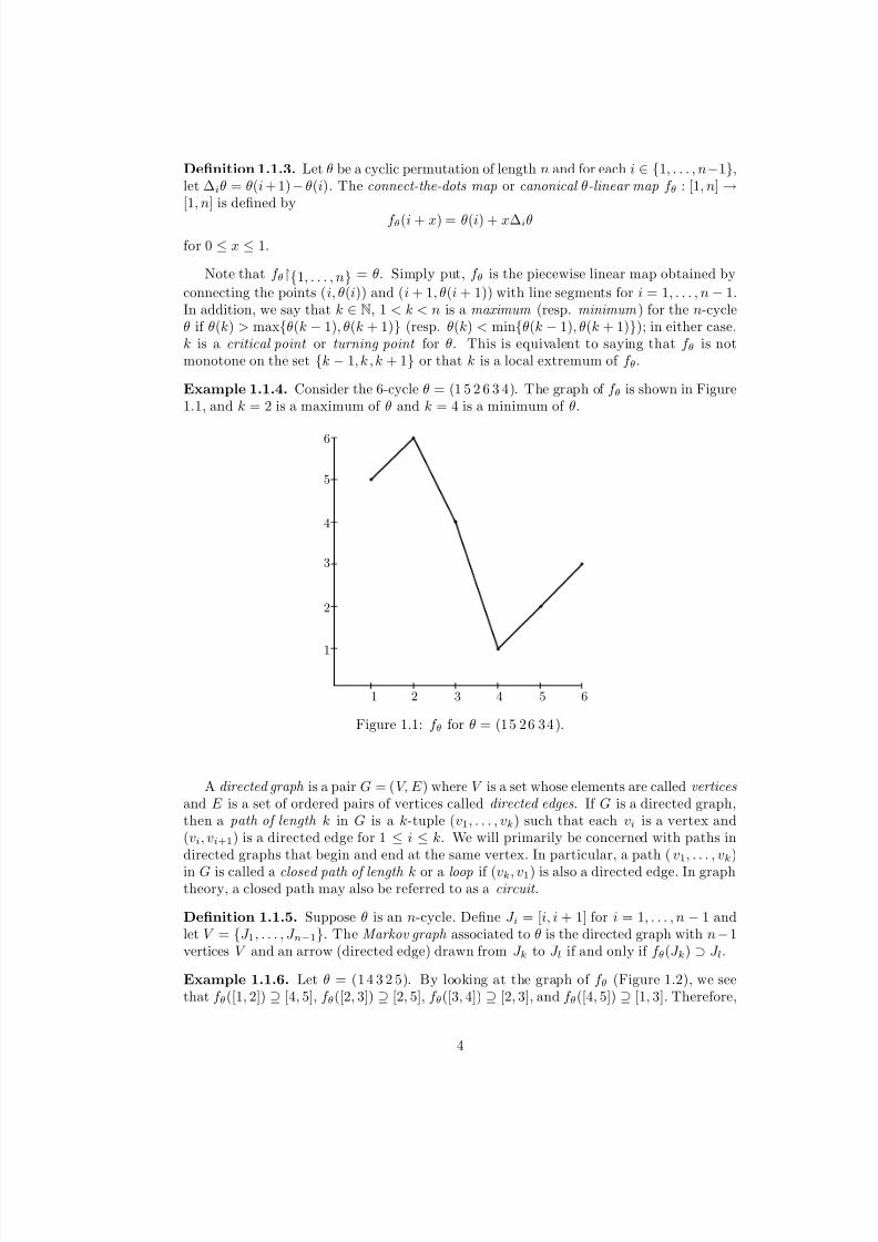
connecting the points (i, θ(i)) and (i + 1, θ(i + 1)) with line segments for i = 1, . . . , n − 1.In addition, we say that k ∈ N, 1 < k < n is a maximum (resp. minimum ) for the n-cycleθ if θ(k) > max{θ(k − 1), θ(k + 1)} (resp. θ(k) < min{θ(k − 1), θ(k + 1)}); in either case,k is a critical point or turning point for θ. This is equivalent to saying that f θ is notmonotone on the set {k − 1, k , k + 1} or that k is a local extremum of f θ.

Example 1.1.4. Consider the 6-cycle θ = (1 5 2 6 3 4). The graph of f θ is shown in Figure1.1, and k = 2 is a maximum of θ and k = 4 is a minimum of θ.

1 2 3 4 5 6

1

2

3

4

5

6

Figure 1.1: f θ for θ = (15 26 34).

A directed graph is a pair G = (V, E ) where V is a set whose elements are called verticesand E is a set of ordered pairs of vertices called directed edges. If G is a directed graph,then a path of length k in G is a k-tuple (v1, . . . , vk) such that each vi is a vertex and(vi, vi+1) is a directed edge for 1 ≤ i ≤ k. We will primarily be concerned with paths indirected graphs that begin and end at the same vertex. In particular, a path (v1, . . . , vk)

in G is called a closed path of length k or a loop if (vk, v1) is also a directed edge. In graphtheory, a closed path may also be referred to as a circuit .

Definition 1.1.5. Suppose θ is an n-cycle. Define J i = [i, i + 1] for i = 1, . . . , n − 1 andlet V = {J 1, . . . , J n−1}. The Markov graph associated to θ is the directed graph with n − 1vertices V and an arrow (directed edge) drawn from J k to J l if and only if f θ(J k) ⊃ J l.

Example 1.1.6. Let θ = (1 4 3 2 5). By looking at the graph of f θ (Figure 1.2), we seethat f θ([1, 2]) ⊇ [4, 5], f θ([2, 3]) ⊇ [2, 5], f θ([3, 4]) ⊇ [2, 3], and f θ([4, 5]) ⊇ [1, 3]. Therefore,

4

8/3/2019 Thesis 4-26-09


the Markov graph of θ has four vertices J i = [i, i + 1] for 1 ≤ i ≤ 4 with directed edgesfrom: J 1 to J 4; J 2 to itself, J 3 and J 4; J 3 to J 2, and from J 4 to J 1 and J 2. This graph isillustrated in Figure 1.3.

1 2 3 4 5

1

2

3

4

5

Figure 1.2: f θ for θ = (1 4 3 2 5).

J 1 J 2

J 3J 4

Figure 1.3: The Markov graph of θ =( 14325) .

Lastly, we remark that if θ ∈ C n, then we will generally consider two different labellingsof the elements of P = { p1, . . . , pn} = {1, . . . , n}. The first is the spatial labeling where

pi < pj if and only if i < j. The second is the temporal labeling where pi = θi−1( p1)for i = 2, . . . , n. Note that the above definition of the temporal labeling is equivalent tosaying pi = θ( pi−1) for i = 2, . . . , n and p1 = θ( pn).

1.2 Continuous Maps of the Interval

We aim to explore the combinatorial properties of periodic points of interval maps. Byan interval map, we mean a continuous function f : I → I of an interval I ⊂ R into itself.Oftentimes, the family of all continuous self-maps of an interval I will be of interest, soX (I ) shall denote this set. Given f ∈ X (I ), we shall examine the iterates f n of f , whichare defined inductively by f 0 = id and f n = f ◦ f n−1 for n ∈ N. For x ∈ I and f ∈ X (I ),the orbit of x under f is defined to be the set

O(x) = {f n(x) : n = 0, 1, 2, . . .}.

A point x is said to be periodic if for some k ∈ N, f k(x) = x. In this case, O(x) is finiteand the set {x, f (x), . . . , f k−1(x)} is called a periodic orbit . The period 1 of a periodic point

x is the least positive integer n such that f n(x) = x; that is, f n(x) = x and f k(x) = x for1 ≤ k ≤ n − 1. We may also call a periodic point of period n an n-periodic point. Lastly,if x is a 1-periodic point, f (x) = x, then we call x a fixed point . Note that an n-periodicpoint x is a fixed point under the map f n, f 2n, f 3n, . . .; however, a fixed point of the mapf n need not be a periodic point of period n.

1In other literature, what we have defined to be the period of a point is sometimes called the least orminimal period.

5

8/3/2019 Thesis 4-26-09


Example 1.2.1. Let θ be an n-cycle. Then it is clear from the definition of θ that{1, 2, . . . , n} is a periodic orbit of period n for f θ.

If P is a nonempty subset of an interval I , then P will denote the closed convex hull of P ; that is, the smallest closed connected subset of I containing P . For example, inR, {2, 3} = 2, 3 = [2, 3] and (1, 5) = [1, 5]. Let f ∈ X (I ) and P = { p1 < · · · pn}be a finite subset of I . We say that f is P -monotone if it is constant on each of thetwo connected components of X \P and f is monotone on each interval [ pi, pi+1] fori ∈ {1, . . . , n − 1}. If I = [1, n] and P = {1, 2, . . . , n}, then the simplest example of aP -monotone map is the connect-the-dots map for some n-cycle θ.

Throughout this paper, a main strategy will be to associate certain directed graphsto interval maps in a way so that the combinatorial properties of the graphs correspondto certain properties of the periodic points of these maps. In particular, given f ∈ X (I ),we aim to show that every loop in the directed graph associated to f corresponds to aperiodic point of f .

Suppose I is an interval, f ∈ X (I ) and J 1 and J 2 are closed subintervals of I . Then,

we say that J 1 f -covers J 2 and write J 1 → J 2 if J 2 ⊂ f (J 1). Our first goal is to show thatthe existence of periodic points under a map f ∈ X (I ) is related to how f acts on closedsubintervals of I .

Lemma 1.2.2. If f is a continuous map and I and J are closed intervals such that f (I ) ⊃ J , then there exists a closed subinterval I ⊂ I such that f (I ) = J , f (int I ) = int J and f (∂ I ) = ∂J .

Proof. Let J = [a, b]. By hypothesis, f (I ) ⊃ J , so there exist points a0, b0 ∈ I such thatf (a0) = a and f (b0) = b. First, let us assume that a0 < b0. Define

a1 = sup{x : a0 ≤ x ≤ b0 and f (x) = a}.

Observe that by continuity, f (a1) = a and since f (b0) = b > a, a1 is strictly less than b0.

Next, defineb1 = inf {x : a1 ≤ x ≤ b0 and f (x) = b},

again noting that f (b1) = b. Now, f ({a1, b1}) = {a, b}, and by definition of a1 and b1, nopoint of (a1, b1) maps to the boundary of J . Thus, f (int(a1, b1)) = intJ = (a, b) and soI = [a1, b1] is the desired subinterval of I . The case when b0 < a0 is handled analogously,interchanging the infimum and supremum.

We shall say that an interval J minimally f -covers an interval I if J satisfies theconclusion of Lemma 1.2.2.

Lemma 1.2.3. If {I k : k = 0, 1, . . .} is a (finite of infinite) family of nonempty closed subintervals of I such that f (I k) ⊃ I k+1 (i.e. I k → I k+1), then there exists a point x ∈ I 0such that f k(x) ∈ I k for each k.

Proof. By Lemma 1.2.2, since f (I 0) ⊃ I 1, there is a closed subinterval J 1 of I 0 thatminimally f -covers I 1. Proceeding by induction, suppose that we have defined subintervalsJ 1 ⊃ J 2 ⊃ · · · ⊃ J n in I 0 such that f k(J k) = I k and J k minimally f k-covers I k for every1 ≤ k ≤ n. Then,

f n+1(J n) = f (f n(J n)) = f (I n) ⊃ I n+1.

Appealing to Lemma 1.2.2, there exists a closed subinterval J n+1 ⊂ J n that minimallyf n+1-covers I n+1, thus f n+1(J n+1) = I n+1. We now have a nested sequence {J n}n∈N of

6

8/3/2019 Thesis 4-26-09


non-empty closed intervals, so the intersection∞n=1 J n is nonempty, and for any x in this

intersection, we have f k(x) ∈ I k.

Lemma 1.2.4. If J ⊂ I is a closed subinterval such that f (J ) ⊃ J , then f has a fixed point in J .

Proof. Let a < b be the endpoints of J . Since f (J ) ⊃ J , there exist points α, β ∈ J suchthat f (α) ≤ a and f (β ) ≥ b. If we let g(x) = f (x) − x, then

g(α) = f (α) − α ≤ f (α) − a ≤ 0

andg(β ) = f (β ) − β ≥ f (β ) − b ≥ 0.

As g is continuous, by the Intermediate Value Theorem, there exists a point x ∈ J suchthat g(x) = 0; that is, x is a fixed point of f .

Before we discuss the implications of the above lemmas, let us first associate to eachinterval map a directed graph which has the property that f -covering relations are encodedas paths.

Given an interval I , a partition is a (finite or infinite) collection of closed subintervals{J k} of I , with pairwise disjoint interiors such that ∪kJ k = I . Given a partition {J k} of I , an interval map f ∈ X (I ) and a point x ∈ I , the itinerary of x of length n is the worditinn(x) = (J i1 , . . . , J in) in the letters {J 1, J 2, . . .}, such that f k(x) ∈ I ik for 1 ≤ k ≤ n.Itineraries give us information about where a point has been and where it might go,without precisely telling us where the point is. Itineraries are very useful tools in symbolicdynamics, and we will revisit their use in later chapters when unimodal permutations arestudied.

Definition 1.2.5. The Markov graph of f ∈ X (I ) associated to the partition {J k} isthe directed graph with vertices J k, and a directed edge from J l to J m if and only if J if -covers J m.

Example 1.2.6. The family of interval maps {qa(x) = ax(1 − x) : a ∈ R} is referredto as the quadratic or logistic family . Consider the partition P = {J 1 = [0, 1/4], J 2 =[1/4, 3/4], J 3 = [3/4, 1]} of the interval [0, 1]. For a = 4, the quadratic map q4(x) =4x(1 − x) maps [0, 1/4] to [0, 3/4], [1/4, 3/4] to [3/4, 1] and [3/4, 1] to [0, 3/4]. The Markovgraph of f associated to the partition P is shown in Figure 1.4.

Example 1.2.7. If we consider the partition of the interval [1, 5] given by P ={[1, 2], [2, 3], [3, 4], [4, 5]}, then for θ = (14325), the Markov graph of f θ associated tothe partition P is the same as in Example 1.1.6. See Figure 1.3. This illustrates that fora connect-the-dots map, Definitions 1.1.5 and 1.2.5 coincide.

Given Definition 1.2.5, Lemma 1.2.3 reveals that every path in the Markov graph of a partition corresponds to a point whose itinerary is exactly the sequence of vertices inthis path. Suppose, in particular, that the path is a closed path, i.e. a path of typeJ i0 → J i2 → · · · → J in−1 → J i0 . Then J i0 f n-covers itself, so Lemma 1.2.4 guaranteesthe existence of a fixed point x ∈ J i0 of f n such that f k(x) ∈ J ik and f n(x) = x. However,if this loop is repetitive in the sense that it is formed by going around smaller loop severaltimes, then the period of the fixed point may be strictly smaller than n. The abovediscussion gives us the following results:

7

8/3/2019 Thesis 4-26-09


0 1

4

3

41

3

4

1

q4

J 3

J 1 J 2

Figure 1.4: The Markov graph of q4(x) associated to the partition P .

Corollary 1.2.8. If J i0 → J i1 → · · · → J in−1 → J n = J i0 is a loop in the Markov graph of f of a partition, then there exists a fixed point x ∈ J i0 of f n with f k(x) ∈ J ik for 0 ≤ k ≤ n − 1.

Lemma 1.2.9. If J i0 → J i1 → · · · → J in−1 → J in = J i0 is a loop in the Markov graph of f of a partition that is not formed by going p times around a shorter loop of length mwhere mp = n, then the periodic point x of Corollary 1.2.8 has period n.

Any loop that cannot be formed by going multiple times around a shorter loop as inthe statement of Lemma 1.2.9 will be called a simple or nonrepetitive loop.

1.3 The Theorem of Sharkovsky

In the previous section, we showed that given an interval map and a partition of theinterval, by analyzing the Markov graph of a partition we can gain useful informationabout the existence of periodic orbits. Suppose now we know that {x1 < · · · < xn} is aperiodic orbit of the interval map f ∈ X (I ). Then, the set P = {[x1, x2], · · · , [xn−1, xn]}is a partition of the interval [x1, xn]. By Lemma 1.2.3, closed paths in the Markov graphof this partition correspond to fixed points of some iterate of f in [x1, xn]. A very naturalquestion then arises: does the existence of a periodic orbit of period n guarantee theexistence of an orbit of some other period? This question was independently answeredby the Ukrainian mathematician Alexander Sharkovsky in two papers between 1964 and1965 [Sha64,Sha65] and by Tien-Yien Li and James A. Yorke in 1975 [LY75].

To address this question, first consider the following ordering ≤s on the natural num-bers defined by:

1 ≤s 2 ≤s 22 ≤s 23 ≤s · · · ≤s 22 · 5 ≤s 22 · 3 ≤s · · ·

≤s 2k · 5 ≤s 2k · 3 ≤s · · · ≤s 2 · 5 ≤s 2 · 3 ≤s · · · ≤s 7 ≤s 5 ≤s 3.

This ordering is eponymously named the Sharkovsky ordering and encodes informationabout which periodic orbits force other periodic orbits to exist. This is stated explicitlyin the following theorem:

8

8/3/2019 Thesis 4-26-09


Theorem 1.3.1 (Sharkovsky). Let m, n ∈ N. Then m ≤s n if and only if every continuousf : I → I having a periodic point of period n has a periodic point of period m.

The proof of this theorem will be given at the end of the paper once the notionsof forcing have been built up sufficiently. Nevertheless, there are several nice proofs of Theorem 1.3.1 that do not use forcing. The standard proof can be found in [BGMY80],whereas slightly different and newer proofs can be found in [ALM93] and [BH]. For theearlier versions, the reader is directed to [Ste77] and [Sha64]. Moreover, both [Mis97],[ALM93] and [BH] describe the rich history of Sharkovsky’s theorem and are interestingreads.

Now, as was mentioned earlier, Li and Yorke came upon a version of Sharkovsky’sresult independently. In their paper, “Period Three Implies Chaos” [LY75], they provedthe following:

Theorem 1.3.2 (Period Three Implies Chaos). If an interval map has a periodic point of period three, then it has a periodic point of period n for each n ∈ N.

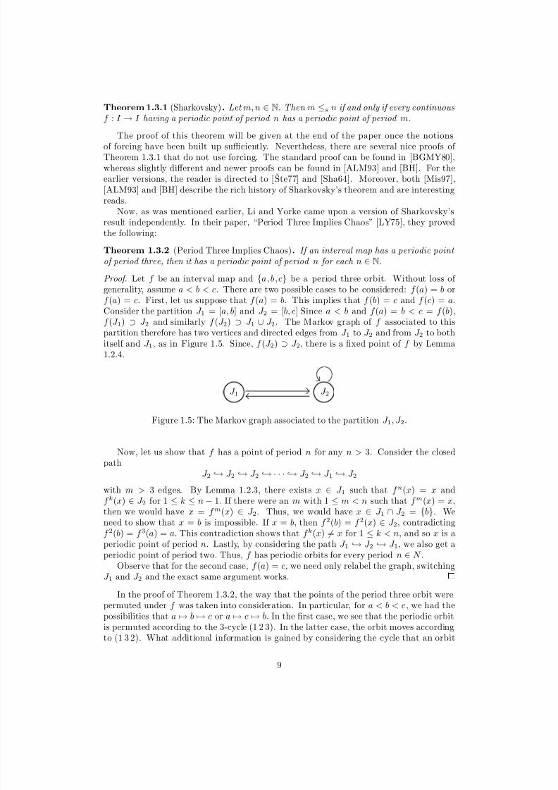
Proof. Let f be an interval map and {a,b,c} be a period three orbit. Without loss of generality, assume a < b < c. There are two possible cases to be considered: f (a) = b orf (a) = c. First, let us suppose that f (a) = b. This implies that f (b) = c and f (c) = a.Consider the partition J 1 = [a, b] and J 2 = [b, c] Since a < b and f (a) = b < c = f (b),f (J 1) ⊃ J 2 and similarly f (J 2) ⊃ J 1 ∪ J 2. The Markov graph of f associated to thispartition therefore has two vertices and directed edges from J 1 to J 2 and from J 2 to bothitself and J 1, as in Figure 1.5. Since, f (J 2) ⊃ J 2, there is a fixed point of f by Lemma1.2.4.

J 1 J 2

Figure 1.5: The Markov graph associated to the partition J 1, J 2.

Now, let us show that f has a point of period n for any n > 3. Consider the closedpath

J 2 → J 2 → J 2 → · · · → J 2 → J 1 → J 2

with m > 3 edges. By Lemma 1.2.3, there exists x ∈ J 1 such that f n(x) = x andf k(x) ∈ J 2 for 1 ≤ k ≤ n − 1. If there were an m with 1 ≤ m < n such that f m(x) = x,then we would have x = f m(x) ∈ J 2. Thus, we would have x ∈ J 1 ∩ J 2 = {b}. Weneed to show that x = b is impossible. If x = b, then f 2(b) = f 2(x) ∈ J 2, contradictingf 2(b) = f 3(a) = a. This contradiction shows that f k(x) = x for 1 ≤ k < n, and so x is aperiodic point of period n. Lastly, by considering the path J 1 → J 2 → J 1, we also get a

periodic point of period two. Thus, f has periodic orbits for every period n ∈ N .Observe that for the second case, f (a) = c, we need only relabel the graph, switching

J 1 and J 2 and the exact same argument works.

In the proof of Theorem 1.3.2, the way that the points of the period three orbit werepermuted under f was taken into consideration. In particular, for a < b < c, we had thepossibilities that a → b → c or a → c → b. In the first case, we see that the periodic orbitis permuted according to the 3-cycle (1 2 3). In the latter case, the orbit moves accordingto (1 3 2). What additional information is gained by considering the cycle that an orbit

9

8/3/2019 Thesis 4-26-09


follows under an interval map? The aim of the next chapter is to make precise this relationbetween periodic orbits and cycles.

10

8/3/2019 Thesis 4-26-09


Chapter 2

The Forcing Relation on Cycles

As was noted in Section 1.3, for interval maps, the existence of a point of period n implies

the existence of periodic points of different periods depending on where n is situated inthe Sharkovsky ordering. If we consider certain combinatorial data found in a periodicorbit, what then, if anything, does this data force an interval map to exhibit? We beginto address this question by first precisely defining what this “combinatorial data” is andthen defining a forcing relation on based on this data.

2.1 The Combinatorial Data in a Periodic Orbit

Suppose f : I → I is a continuous map of a closed interval I . The theorem of Sharkovsky(Theorem 1.3.1) tells us that the existence of a point of period n under f implies theexistence of a point of period m for every m ≤s n. The only information that this theoremuses is the existence of a point of period n. However, we often know more. Suppose x is

a periodic point of period n. Label the points in the orbit of x from left to right, so thatO(x) = {x1, . . . , xn} with x1 < · · · < xn. Then, in addition to the fact that x is a pointof period n under f , we know how f permutes the set {x1, . . . , xn}; namely, there existsan n-cycle θ such that f (xi) = xθ(i) for i = 1, . . . , n.

Definition 2.1.1. If θ is an n-cycle, f : I → I a continuous map of a closed interval, andX = {x1, x2, . . . , xn} ⊂ I with x1 < · · · < xn, then we say X is an orbit of type θ (or X exhibits θ) if f (xi) = xθ(i), 1 ≤ i ≤ n. In addition, f is said to exhibit the n-cycle θ if there exist x1 < · · · < xn such that {x1, . . . , xn} is an orbit of type θ. We will denote theset of all permutations exhibited by f by Perm(f ).

Example 2.1.2. The symmetric family of tent maps {T a}a∈[0,2] is given by T a(x) = ax for

x ∈ [0, 12 ] and T a(x) = a(1− x) for x ∈ [ 1

2 , 1] [BB04]. For two values of a, a = a1 ≈ 1.72208

and a = a2 ≈ 1.51288, x0 =

1

2 is a periodic point of period 5 for the tent maps T a1 and T a2 .Denote the period 5 orbit for each map by x0, x1, x2, x3, x4 with xi → xi+1. Relabeling thepoints in a linearly increasing manner, the permutations exhibited are obtained. As canbe seen in Figure 2.1 [BB04, Figure 3.3], T a1 exhibits the permutation (1 2 4 3 5) whereasT a2 exhibits the permutation (1 3 4 2 5).

Definition 2.1.1 points towards a generalization of the Sharkovsky ordering, one thatconsiders orbit types. Example 2.1.2 shows that we may certainly have two distinct pe-riodic orbits of period 5. In fact, a simple counting argument shows us that there are

11

8/3/2019 Thesis 4-26-09


x2 x3 x0 x4 x1

1

2

1 2 3 4 5

( 12435)

T a1

x2 x0 x3 x4 x1

1

2

1 2 3 4 5

( 13425)

T a2

Figure 2.1: Graphs of symmetric tent maps exhibiting different 5-cycles.

(n − 1)! possible distinct orbit types for a periodic point of period n. In our more generalsetting, what does the existence of a periodic orbit of type θ imply? This motivates thefollowing definition.

Definition 2.1.3. Let θ and η be cycles. We say θ forces η, denoted θ→η, if everycontinuous map f : I → I that has an orbit of type θ also has an orbit of type η.Equivalently, θ→η if {f : θ ∈ Perm(f )} ⊂ {f : η ∈ Perm(f )}.

A priori , Definition 2.1.3 merely defines a relation, that is, a subset of C × C . Theusefulness of this definition thus depends on how we can characterize this relation. First,recall the definition of a partial order:

Definition 2.1.4. A partial order is a relation on a set X that is reflexive, transitive andantisymmetric. A set equipped with a partial order is called a partially ordered set .

As it turns out, forcing is a partial order on the set of cycles C but not a linear ordering.

Theorem 2.1.5 ([Bal87, Theorem 1.4]). Forcing is a partial order.

Proof. We need to show that → is a reflexive, transitive and antisymmetric relation. Letθ, η and τ be cycles. Reflexivity is trivial: if a map exhibits θ, then it exhibits θ. Hence,θ→θ. For transitivity, suppose θ→η and η→τ . If a map exhibits θ, then it exhibits η, andsince it exhibits η, it exhibits τ . Thus, we have θ→τ and so → is a transitive relation.

Antisymmetry, on the other hand, requires a bit more work. Let n, m ∈ N and θ ∈C n, η ∈ C m. Suppose that θ→η and η→θ. We aim to show that this implies θ = η.Following [Bal87] and [ALM93, p.53], let f be a polynomial of degree at least 2 whichpasses through all of the points (i, θ(i)) for 1 ≤ i ≤ n, so that f has an orbit of type θ(and therefore, by hypothesis, an orbit of type η). Now, as f is a polynomial, the equationf n(x) = x has only finitely many solutions, so f can have only finitely many orbits of typeθ. Let P = {x1, . . . , xn}, x1 < · · · < xn, be one of these orbits having the property that

12

8/3/2019 Thesis 4-26-09


max P − min P = xn − x1 is the least possible. Define a continuous function g by

g(x) =

f (x1) : x ≤ x1

f (x) : x ∈ [x1, xn]f (xn) : x ≥ xn

By construction, g has an orbit of type θ, namely P , and therefore, by hypothesis, has anorbit of type η, say Q = {y1, . . . , ym}, y1 < · · · < ym. Note that since g(P ) = P and forall x /∈ [x1, xn], g(x) ∈ P , we have Q ⊂ [x1, xn]. By the same construction as above, thereis a continuous map h given by

h(x) =

f (y1) : x ≤ y1

f (x) : x ∈ [y1, ym]f (ym) : x ≥ ym

Since Q is an orbit of type η for h, h must also have an orbit of type θ, say R = {x1, . . . , xn}.

But, R ⊆ [y1, ym], so R is also an orbit of f of type θ. By the minimality of P , we haveR = P , so P = Q and thus θ = η.

Theorem 2.1.6 ([Bal87, Theorem 1.5]). Forcing is not a linear ordering.

Proof. To show that forcing is not a linear ordering it suffices to show that there existtwo cycles θ and η such that θ→η and η→θ. By definition of the forcing relation, it issufficient to show that there exist two continuous maps, one exhibiting θ but not η, andthe other exhibiting η but not θ. To that end, let θ = (12 3) and η = (1 3 2) and recall thedefinition of the connect-the-dot maps f θ and f η (Definition 1.1.3, see Figure 2.2).

First, suppose that f θ exhibits η. Consider the partition {J 1, J 2} of [1, 3] with J i =[i, i + 1] and let P = {x1 < x2 < x3} be the periodic orbit of period three that exhibitsη, i.e., x1 → x3 → x2 → x1. Clearly P = {1, 2, 3}, otherwise θ would equal η. Sincex1 < x2 and f θ(x1) = x3 > x1 = f θ(x2), we must have that x1 ∈ J 2. Similarly, as x2 < x3

and f θ(x2) = x1 < x2 = f θ(x3), x2 must be in J 1. But, as x2 = 2, this contradicts ourassumption that x1 < x2. Thus, f θ is a continuous map that exhibits θ but not η, soθ→η. This amounts to the fact that there are no three points x1 < x2 < x3 such thatf θ(x2) < f θ(x3) < f θ(x1).

On the other hand, suppose that f η exhibits θ. The reasoning is almost identicalto the first case. Using the same partition of [1, 3], this time let Q = {y1 < y2 < y3}denote the period three orbit that exhibits θ, so that y1 → y2 → y3 → y1. Again, notethat Q = {1, 2, 3} otherwise η would be the same permutation as θ. Now, y1 < y2 andf η(y1) = y2 < y3 = f η(y2) so y1 ∈ J 2. However, y2 < y3 and f (y2) = y3 > y1 = f (y3), soy2 ∈ J 1. This again contradicts the assumption that y1 < y2. Therefore, f η is a continuousmap that exhibits η but not θ, so η→θ. This concludes the proof of showing that forcingis not a linear ordering.

2.2 The Forcing Theorem

Thus far, we have shown that the set C of cycles is partially ordered by the forcingrelation →, and moreover, this relation is not a linear ordering. Nevertheless, a criterionfor deciding when a cycle θ forces another cycle η has yet to be given. The main goalof this section, therefore, is to state and prove the Forcing Theorem (Theorem 2.2.1)which gives a necessary and sufficient condition for a cycle to force another. First proven

13

8/3/2019 Thesis 4-26-09


1 2 3

1

2

3

1 2 3

1

2

3

f θ f η

Figure 2.2: Graphs of f θ and f η.

in [Bal87, Main Theorem 2.4], this theorem and its proof plant the seeds for Chapter 3where an explicit algorithm is presented that decides the forcing relation.

Theorem 2.2.1 (Forcing Theorem). If θ ∈ C n and η ∈ C m, then θ→η if and only if either θ = η or there is a loop of length m in the Markov graph of θ with orbit type η.

To begin with, it is clear that given some cyclic permutation θ, the family of intervalmaps that exhibits θ can be extremely large. An interesting question is then whether ornot there exists some canonical interval map that exhibits only the cyclic permutationsforced by θ. If this were to be the case, then we could reduce forcing to the study of properties of these maps alone. In particular, our approach will be to show that suchcanonical maps exist – indeed, they are the connect-the-dots maps from Chapter 1 – and

that by studying the combinatorial properties of the Markov graphs of these maps, thedesired criterion for forcing can be derived.Let θ ∈ C n and consider the interval map f θ. Observe that to every vertex I in

the Markov graph of θ (equivalently, the Markov graph of f θ associated to the partition{[1, 2], . . . , [n − 1, n]}, see Example 1.2.7), we can assign a sign that is either +1 or −1depending on whether f θ is increasing or decreasing, respectively, on I . The function thatassigns to a vertex its sign will be denoted by z. Therefore,

z(I ) =

+1 if f θ increasing on I −1 if f θ decreasing on I

Example 2.2.2. The graph of f θ and the signed Markov graph of θ are shown in Figures2.3 and 2.4, respectively, for θ = (1 4 3 25).

Now, in Chapter 1 it was shown that a simple loop of length n in the Markov graphof an interval map corresponds to an n-periodic point of the map. This periodic pointnecessarily has an orbit type of θ for some n-cycle θ, so the question arises how do werecover the orbit type from the simple loop? The key lies in studying the signs of thevertices of the loop. We aim to introduce an ordering < on loops of the same length in agiven Markov graph in such a way that the order of the real line is reflected in the orderof the loops.

14

8/3/2019 Thesis 4-26-09


1 2 3 4 5

1

2

3

4

5

Figure 2.3: f θ for θ = (1 4 3 2 5).

J 1,+ J 2,−

J 3,+J 4,−

Figure 2.4: The signed Markov graph of θ =( 14325) .

Definition 2.2.3. For a loop (J i1 , . . . , J in), we define the shift operation σ by σ(J i1 , . . . , J in) =(J i2 , J i3 , . . . , J in , J i1). Given two loops α = (J i1 , . . . , J in) and β = (J k1 , . . . , J kn) of thesame length, we define α < β if and only if

M −1

j=1

z(J ij )

iM <

M −1

j=1

z(J ij )

kM ,

where M ≤ n is the least value of j for which ij = kj . This is a linear ordering.

When we are dealing with the Markov graphs of cycles (resp. connect-the-dots maps)it will be notationally easier sometimes to label the vertices as integers. Thus, insteadof labeling the n − 1 vertices of the Markov graph of an n-cycle by J 1, J 2, . . . , J n−1, wewill simply label them 1, 2, . . . , n − 1, where the integer i corresponds to the subinterval[i, i +1]. Then, if α = (a1, a2, . . . , an) and β = (b1, b2, . . . , bn) are loops of the same length,we have α < β if and only if

M −1

j=1

z(aj)

aM <

M −1

j=1

z(aj)

bM .

where M ≤ n is the least value of j for which aj = bj .The most important aspect of this ordering is the following: suppose f ∈ X (I ) is an

interval map, J 1, . . . , J N is a partition of I (labeled so that min J i < min J i+1) and wehave loops α = (J i1 , . . . , J in) and β = (J k1 , . . . , J kn) in the Markov graph of f associatedto this partition. These loops can be thought of as signed itineraries of periodic pointsin I , say x corresponding to α and y corresponding to β . We will see in the proof of theforcing theorem that the order of loops tells us the order of the points to which the loopscorrespond:

Proposition 2.2.4. α < β implies x < y.

15

8/3/2019 Thesis 4-26-09


Example 2.2.5. In the Markov graph of θ = (1243) (Figure 2.5), one can find thenonrepetitive loops (1, 2, 2), (2, 2, 1) and (2, 1, 2). Using the order from Definition 2.2.3,observe that (1, 2, 2) < (2, 2, 1) and (1, 2, 2) < (2, 1, 2) because +1 < +2 as integers.

Because the sign of the vertex 2 in the Markov graph of θ is negative, we have (2, 2, 1) <

(2, 1, 2), since −2 < −1 as integers. Thus, we have (1, 2, 2) < (2, 2, 1) < (2, 1, 2).

1, + 2, −

3, +

Figure 2.5: Markov graph of θ = (1 2 4 3)

Definition 2.2.6. Let be a nonrepetitive loop of length m and let W = {, σ(), σ2(), . . . , σm−1()}.Order W by < and let ord : W → {1, . . . , m} be the unique one-to-one order preservingfunction. We define the orbit type or loop type of W to be the cycle θ that is defined by

θ(i) = ord ◦ σ ◦ ord−1, 1 ≤ i ≤ m.

If α is any loop, then we define the orbit type of α to be the orbit type of W where W

is the smallest such that α ∈ W and W is closed under σ. With this definition, the orbittype of α is equal to the orbit type of σ(α).

Example 2.2.7. Let W = {(1, 2, 2) < (2, 2, 1) < (2, 1, 2)} be the ordered collectionof loops of length 3 given in Example 2.2.5. We want to decide the orbit type θ of this ordered list of shift equivalent loops. Definition 2.2.6 tells us that for i = 1, 2, 3,θ(i) = (ord ◦ σ ◦ ord−1)(i). Thus, for i = 1, we have

θ(1) = ord(σ(ord−1(1))) = ord(σ((1, 2, 2))) = ord((2, 2, 1)) = 2.

Similarly, for i = 2 and i = 3, we get θ(2) = 3 and θ(3) = 1. Thus, the orbit type of W is(123).

Now we are ready to prove half of the Theorem 2.2.1.

Proposition 2.2.8 ([Bal87, Lemma 3.1]). If θ ∈ C n and f θ has an orbit of type η, then either θ = η or the there is a loop in the Markov graph of θ that has orbit type η.

Proof. Following [Bal87, Lemma 3.1]: Let X = {x1, x2, . . . , xm} be an orbit of type η withx1 < x2 < · · · < xm and note that by definition of f θ we must have 1 ≤ x1 and xm ≤ n.Assume θ = η, so that none of x1, . . . , xm are integers. Define the path α = (a1, . . . , am)in the Markov graph of θ by

aj = i ⇐⇒ f jθ (x1) ∈ [i, i + 1],

16

8/3/2019 Thesis 4-26-09


and observe that α is actually a loop in the Markov graph of θ. We first want to showthat α is nonrepetitive, so suppose that β is a loop in the Markov graph of θ of lengthk such that k divides m and aj1 = bj2 if and only if j1 ≡ j2(mod k). Define intervals

I j , 0 ≤ j ≤ m by backwards induction from m. Let I m = [am, am + 1], and if I j hasbeen defined for j ≥ 1, let I j−1 = f −1

θ (I j) ∩ [aj−1, aj−1 + 1] (where we let a0 = amfor convenience). Now aj−k = aj , so we can show by induction that I j−k ⊆ I j wheneverk ≤ j ≤ m and that f kθ is a one-to-one linear function from I j onto I j+k (1 ≤ j,j +k ≤ m).Since I 0 ⊆ I k, f kθ : I 0 → I k has a fixed point y, and clearly f m(y) = y also, since k divides

m. However, x1 ∈ I 0 (since by definition f jθ (x1) ∈ [aj , aj+1] for all j) and f mθ (x1) = x1,but x1 = y (since x1 has least period m and y has least period k < m). Thus f mθ : I 0 → I mis one-to-one, onto, linear, and has two fixed points, so I 0 = I m and f mθ is the identityfunction. Furthermore, since |f θ(x)| ≥ 1 whenever f θ(x) is defined and 1 < x < n, wehave I j = [aj , aj + 1] for all j and f kθ : I j → I j+k is a linear map of slope either 1 or −1.Thus if x1 = am + 1

2 , then f kθ (x) = am + 12 contradicting x1 has least period m > k , and

if x1 is some element of [am, am + 1] other than am + 12 , then it is easy to see that X has

type θ, contradicting θ = η. Thus α must be nonrepetitive.Next, we must show that the orbit type of α equals η. Let α(k) = σk(α) with α(k) =

(a1(k), a2(k), . . . , am(k)) and note that aj(k) = i if and only if f j+kθ (x1) ∈ [i, i + 1].

Suppose α(k1) < α(k2). Let j be least such that aj(k1) = aj(k2). Then if we look

at f k1θ (x1) and f k2θ (x1) and follow their progress as f θ is repeatedly applied j times, wesee that they switch order if and only if z(aj(k1)) is −1 an odd number of times. But

since f jθ (f k1θ (x1)) ∈ [aj(k1), aj(k1) + 1] and f jθ (f k2θ (x1)) ∈ [aj(k2), aj(k2) + 1] we see that

f k1θ (x1) < f k2θ (x1).Thus we have shown that

f k1θ (x1) < f k2θ (x1) ⇐⇒ α(k1) < α(k2),

from which it follows that the orbit type of α is η.

Now we need to show the other direction: if there is a loop in the Markov graph of θof loop type η, then any interval map with an orbit of type θ has an orbit of type η. First,we need to prove the following lemma:

Lemma 2.2.9 ([Bal87, Lemma 3.2]). Suppose that f : R → R is continuous, a < b,f (a) < f (b), and for some N ∈ N, {(ai, bi) : 1 ≤ i ≤ N } is a collection of intervals having the properties that

(i) f (a) ≤ f (ai) < f (bi) ≤ f (b);

(ii) a ≤ ai < bi ≤ b;

(iii) (ai, bi) minimally f -covers itself;

(iv) If i < j, then either (aj , bj) ⊆ (ai, bi) or (ai, bi) ∩ (aj , bj) = ∅;

(v) f is strictly increasing on the set {ai : i < N } ∪ {bi : i < N }.

If c < d, c, d ∈ [f (a), f (b)] are such that for all i either (c, d) ⊆ (f (ai), f (bi)) or (c, d) ∩ (f (ai), f (bi)) = ∅, then there exist points aN +1 and bN +1 such that f (aN +1) =c, f (bN +1) = d and {(ai, bi) : 1 ≤ i ≤ N + 1} satisfies (i)-(v) with N replaced by N + 1.

17

8/3/2019 Thesis 4-26-09


Proof.Case 1. (c, d) ⊂ (f (ai), f (bi)) for some i.

Assume that i is the largest possible, so that (f (ai), f (bi)) ⊂ (f (aj), f (bj)) or

(f (ai), f (bi)) ∩ (f (aj), f (bj)) = ∅ for all i = j (by condition (iv) and (v)). Let aN +1

be the greatest element of [ai, bi] such that f (aN +a) = c and then let bN +1 be the leastelement of [aN +1, bi] such that f (bN +1) = d.Case 2. (c, d) ∩ (f (ai), f (bi)) = ∅ for all i.

Now let a be the greatest element of {a} ∪ {bi : f (bi) ≤ c} and let b be the leastelement of {b} ∪ {ai : f (ai) ≥ d}. Let aN +1 be the greatest element of [a, b] such thatf (aN +1) = c and let bN +1 be the least element of [aN +1, b] such that f (bN +1) = d.

In either case the appropriate choice of aN +1 and bN +1 will work.

Proposition 2.2.10 ([Bal87, Theorem 3.3]). If f is an interval map having an orbit of type θ ∈ C n and α is a loop in the Markov graph of θ of loop type η ∈ C m, then f has an orbit of type η.

Proof. Let P = { p1 < · · · < pn} be an orbit of type θ for f , and let α = (a1, a2, . . . , am)be a nonrepetitive loop of length m in the Markov graph of θ. Let us define integersaj for j ∈ {0, m + 1, m + 2, . . . , 2m − 1, 2m} by a0 = am and aj = aj−m; that is,am+1 = a1, am+2 = a2, etc. For i ∈ {1, . . . , n − 1}, define I i to be the interval [xi, xi+1].We want to define a collection of 2m + 1 intervals J i, 0 ≤ i ≤ 2m which satisfy thehypotheses of Lemma 2.2.9. To do so, first let J 2m = I am. Suppose by induction thatJ j+1, J j+2, . . . , J 2m have been defined with J i ⊆ I ai and that if j + 1 ≤ i < k ≤ 2m theneither J i ⊆ J k or J i ∩ J k has at most one point. Assume also as part of the inductionhypothesis that J i minimally f -covers J i+1 for j + 1 ≤ i ≤ 2m − 1. If we consider theintervals J i, j + 1 ≤ i ≤ 2m − 1 such that J i ⊆ I ai and J i+1 ⊆ I aj+1 , then we see thatLemma 2.2.9 applies (using either f or −f , depending on whether f (xaj ) < f (xaj+1) orvice versa) in order to get J i ⊆ I aj with f taking J j onto J j+1 with the other claims of the induction hypothesis holding. Therefore, we get that J 0 ⊂ J m and f m takes J 0 onto

J m, so by Lemma 1.2.4, f m

has a fixed point y ∈ J 0.

Case 1. For some 0 < i < j ≤ m, J i ∩ J j = ∅Now, J i ⊆ J j is impossible, since then we would have J i+k ⊆ J j+k for all 0 ≤ k ≤ m

which would imply that ai+k = aj+k (since J k ⊆ I ak), contradicting that α is nonrepeti-tive. Thus J i and J j intersect at a single point, say J i ∩ J j = {x}, so by construction of the J k’s, J i+k ∩ J j+k is a single point for all 0 ≤ k ≤ 2m − j, in particular J i+2m−j ∩ J 2m isa single point, namely either aa2m or pa2m+1, so J i+k ∩ J j+k is a point of P for all such k.Thus, since the induction used 2m steps and 2m − j ≥ m, f k( p1) = x for some k ≤ m, sothere is a k such that J i+k ∩ J j+k = { p1}, which is impossible since J i+k ∪ J j+k ⊆ [ p1, pn].Thus Case 1 leads to a contradiction.

Case 2. If 0 < i < j ≤ m, then J i ∩ J j = ∅.

Then if J i ∩ J j ⊆ I k for some fixed k, then by the construction of J i, J i+1 and J j+1

stay in the same order as J − i and J − j if f ( pk) < f ( pk+1) and J i+1 and J j+1 switchorder compared to J i and J j if f ( pk) > f ( pk+1). The same argument used at the end of Proposition 2.2.8 now gives that {f k(y) : 1 ≤ k ≤ m} is an orbit of f of type η.

Thus, Propositions 2.2.8 and 2.2.10 prove both directions of the Forcing Theorem.Before moving onto the next section, let us briefly discuss the implications of Theorem

2.2.1. In Section 2.1, forcing was defined as a property of all interval maps exhibitinga certain cycle: θ→η if and only if every continuous map that exhibits θ exhibits η. In

18

8/3/2019 Thesis 4-26-09


this respect, Theorem 2.2.1 is remarkable: forcing can be reduced to simply studyingcombinatorial properties of cycles and their Markov graphs. To decide whether or not agiven cycle θ forces another cycle η, the only continuous function that we need to consider

is f θ, and we need only consider this function so that we can construct the Markov graphof θ. However, the function f θ is merely a convenience, since we could easily constructthe Markov graph of θ directly from properties of θ. Therefore, in a sense, one could poseforcing as an intrinsic order on the set of cyclic permutations, an order independent of anyrelation to continuous maps and dynamical systems all together.

19

8/3/2019 Thesis 4-26-09


Chapter 3

A Computational Digression

Having defined the partial order → on the set of all cyclic permutations and stated and

proven the forcing theorem (Theorem 2.2.1), we will now give an algorithm which describesforcing. In [Bal87], Baldwin derives an explicit combinatorial algorithm which decides allm-cycles that a given n-cycle forces. From this, one can clearly extend the algorithmas follows: input an integer m and an n-cycle θ and return all k-cycles forced by θ for1 ≤ k ≤ m. Additionally, one can make slight modifications so that a user may inputcycles θ and η and ask if θ→η. We give a thorough description of Baldwin’s algorithmas well as our own implementation of the algorithm in the algebra system GAP and theresults obtained.

3.1 Description of the Algorithm of Baldwin

The proof of Theorem 2.2.1 essentially gives us the desired algorithm: a necessary and

sufficient condition for θ to force η is that there is a closed loop of length |η| in the Markovgraph of θ that has loop type η. Therefore, we can describe the algorithm as follows:

1. Input a cyclic permutation θ ∈ C n and an integer m.

2. Construct the Markov graph of θ and find all closed paths (loops) of length m inthis graph.

3. Partition the family of closed paths of length m into sets equivalent under the shiftoperation.

4. Compute the orbit type of each shift equivalent set. This will give all η ∈ C m forcedby θ.

Example 3.1.1. Let us find all of the 3-cycles forced by θ = (12 4 3). To that end, weneed to first construct the Markov graph of θ (Figure 2.5) and then find all (non-trivial)loops of length 3. Up to equivalence modulo the shift operation, there are four relevantloops, namely L1 = (1, 2, 2), L2 = (3, 2, 2), L3 = (1, 2, 3) and L4 = (1, 3, 2). Let us analyzethese loops one at a time.

L1: From Example 2.2.5, the ordered list of loops that are shift equivalent to L1 is(1, 2, 2) < (2, 2, 1) < (2, 1, 2), and from Example 2.2.7, the orbit type of thisordered list is (1 2 3). Therefore, we conclude that θ→(123).

20

8/3/2019 Thesis 4-26-09


8/3/2019 Thesis 4-26-09


an orbit of type η. Recall from Definition 2.1.3 that forcing is defined as a property of all continuous maps exhibiting a certain cyclic permutation. In fact, there is an inherentproblem with using the connect-the-dots maps to determine forcing. The problem with

using f θ as the model map is that, although the set of representatives of η in f θ is inone-to-one correspondence with a subset of the closed paths of length |η| in the Markovgraph of θ, there is no efficient way known of determining whether η has a representativein f θ. Baldwin solved this problem by ignoring it. In his algorithm, one examines all closed paths of length |η| in the graph to see if any of them correspond to a representativeof η. The number of such paths is exponential in |η| [BCMM92].

However, it is possible to speed up the algorithm considerably. In [BC92a], Bernhardtand Coven present an effective polynomial-time algorithm for deciding forcing. This paper,which can be seen as an extension of [BCMM92], considers horseshoe maps instead of connect-the-dots maps.

Definition 3.3.1. Let θ be an n-cycle and let M be the number of nondegenerate intervalsI maximal with respect to “f θ is strictly monotone on I ” (such intervals are called laps).

The horseshoe map of θ is the map H θ : [0, 1] → [0, 1] defined as follows: H θ(0) = 0or 1 according to whether θ(1) < θ(2) or θ(1) > θ(2), and H maps each subinterval[(i − 1)/M, i/M ] linearly onto [0, 1] for i = 1, . . . , M − 1.

The essential idea to check whether θ forces η is to first find a certain canonical repre-sentative, say Q, of θ in H θ. Then, θ forces η if and only if H θ has a representative P of η such that

minq∈Q

q −i

M

≤ min p∈P

p −i

M

, i = 1, . . . , M − 1.

This algorithm is similar to an earlier one given by Jungreis [Jun91] which useditineraries of points.

3.4 Properties of Forcing in the diagrammed data

To begin with, Baldwin’s original diagram [Bal87, Figure 4], showing the forcing relationon all 36 cycle of length up to 5, is shown in Figure 3.1. In Figure 3.2, the forcing relationon almost 200 cycles of order up to 8 has been diagrammed. This diagram contains the 36cycles from Baldwin’s original diagram of forcing on all cycles of length up to 5. We adoptthe convention that θ→η if and only if θ is above η and there is a line segment betweenθ and η. There are several aspects of this diagram which warrant being pointed out, asthey will be described at length in later chapters. The first clear property of Figure 3.2is that it is symmetric about a vertical axis extending from (1 2). This symmetry couldsimply be an artifact of the way in which the forcing relations were diagrammed; however,we will show in Chapter 4.1 that this is not the case. In fact, in Proposition 4.1.4, we will

prove that for every cycle θ there exists a cycle θ with the property that θ forces η if andonly if θ forces η.Though more subtle than the symmetry in Figure 3.2, one characteristic is that there

is a “long vein” of cycles on which the forcing relation is a linear ordering; that is, for anytwo cycles in this vein, θ forces η or η forces θ. We will outline in Chapter 4.2 that theforcing relation restricted to unimodal cycles is a linear ordering.

Lastly, of the cycles that have been diagrammed, if one looks at the lengths of thecycles “immediately above” a given cycle θ (Definition 5.1.5), then the length turns outto be 2|θ|. In Chapter 5.1, we will prove that immediately above any cycle lies all of

22

8/3/2019 Thesis 4-26-09


Figure 3.1: Baldwin’s original diagram.

its doubles. Consequently, we note that the forcing order on cycles is not locally finite:between any two odd length cycles lie infinitely many even length cycles.

23

8/3/2019 Thesis 4-26-09


Figure 3.2: Computation of → for n ≤ 8.

24

8/3/2019 Thesis 4-26-09


Chapter 4

Global Structure of Forcing

In application, one major difference that the ordering → has when compared to the

Sharkovsky ordering, is that forcing is only a partial ordering (Theorem 2.1.6). Whereasany pair of elements in N are mutually comparable under the Sharkovsky ordering (thatis, ≤s is a linear ordering), this need not hold for any pair of elements in C under →. Forexample, consider the 4-cycles (1 2 3 4) and (1 4 3 2). It can be shown (see Chapter 3) thatthe only 4-cycle that (12 3 4) forces is (1 3 2 4), and the only 4-cycle that (1 4 3 2) forcesis (1423). Thus, (1234)→(1 4 3 2) and (14 3 2)→(1 2 3 4). However, the 4-cycle (1 2 4 3)forces both (1423) and (1324), yet is incomparable with both (1234) and (1432)!These relationships are illustrated in Figure 4.1.

( 1234)

( 1243)

( 1432)

(1 3 2 4) (1 4 2 3)

Figure 4.1: Illustration of the complexity of → on some 4-cycles.

This one example begins to illustrate the complex global structure of ( C, →). However,there is some symmetry and “nice” structure to (C, →) when we either consider certainpairs of cycles or restrict ourselves to certain types of cycles.

4.1 The Flip Symmetry

One distinctive characteristic of Figure 3.2 is that it is symmetric about a vertical axisextending from (1 2). The aim of this section is to show that to every cycle θ we can asso-

25

8/3/2019 Thesis 4-26-09


ciate a cycle θ with the property that θ→η if and only if θ→η. Therefore, by diagrammingθ and θ across from each other, we obtain a sort of global symmetry in (C, →).

Definition 4.1.1. Given θ ∈ C n, the flip of θ, denotedˆθ, is defined to be the n-cycle suchthat θ(k) = n + 1 − θ(n + 1 − k).

Example 4.1.2. Consider the 4-cycle θ = (1 3 2 4). The flip of θ is defined by

θ(1) = 4 + 1 − θ(4 + 1 − 1) = 4

θ(2) = 4 + 1 − θ(4 + 1 − 2) = 3

θ(3) = 4 + 1 − θ(4 + 1 − 3) = 1

θ(4) = 4 + 1 − θ(4 + 1 − 4) = 2

Thus, θ = (1423).

Example 4.1.3. As Figure 3.2 would suggest, the flip of a cycle θ may equal θ. Indeedfor the cycles (1 2), (12 4 3) and (14 7 3 8 5 2 6) this is precisely the case.

We have chosen to call θ the flip for the following reason: the graph of the connect-

the-dots map f θ is a 180◦ rotation of the graph of the map f θ. A consequence of thisobservation is that the Markov graph of θ is obtained from the Markov graph of θ byrelabeling the vertex i by n − i.

Proposition 4.1.4 ([Bal87, Proposition 4.2], [ALM93, Proposition 2.4.6]). Let θ, η ∈ C .

Then, θ→η if and only if θ→η.

Proof. Let θ ∈ C n and suppose that θ→η for some cycle η. Let h : [1, n] → [1, n] be theorientation-reversing homeomorphism h(x) = −x + n + 1. Then h ◦ f θ ◦ h−1 = f θ. Thiscan be seen by the fact that for any k ∈ {1, . . . , n},

(h ◦ f θ ◦ h−1)(k) = h(f θ(h−1(k)))

= h(f θ(n + 1 − k)) def. of h

= h(θ(n + 1 − k)) def. of f θ= h(n + 1 − θ(k)) def. of θ

= −(n + 1 − θ(k)) + n + 1

= f θ(k).

Since f θ is linear on each interval of the form (k, k +1) for k ∈ {1, . . . , n − 1}, we conclude

that h ◦ f θ ◦ h−1 is also linear on each such interval and “connects the dots” (k, θ(k)).Thus, this map is indeed f θ. Now, if X is the orbit of type η for f θ, then it follows fromthe above construction that (h ◦ f θ ◦ h−1)(X ) is an orbit of type η for f θ. Therefore,

by Theorem 2.2.1, θ→η. By using the same h, but starting with f θ, we get the other

direction. Thus, θ→η if and only if θ→η.

Corollary 4.1.5. [ALM93, Corollary 2.5.7] A cycle either is equal to its flip or does not force its flip.

4.2 The Restriction of Forcing to Unimodal Permuta-

tions

The aim of this section is to prove that forcing is a linear ordering when restricted to acertain family of cyclic permutations called unimodal cycles. To fully develop the theory

26

8/3/2019 Thesis 4-26-09


necessary to show this would require a lot of new notation that is ultimately not used inthe remaining chapters, so this section is incomplete in that respect. Nevertheless, for anyresult that is unproven, citations will be given where the interested reader may find the

proofs.By a unimodal map f , we mean an interval map that is continuous, has exactly one

critical point and is strictly increasing (resp. decreasing) left (resp. right) of the criticalpoint. Examples of unimodal maps include quadratic maps and tent maps of the interval.The definition of a unimodal cycle follows naturally from the definition of a unimodalmap:

Definition 4.2.1. A unimodal cycle is a cycle θ such that f θ is a unimodal map. Denotethe set of all unimodal n-cycles by U n.

Example 4.2.2. For any n ∈ N, the cycle (123 · · · n − 1 n) is unimodal. In particular,the 5-cycle θ = (1 2 3 4 5) is a unimodal cycle and its connect-the-dots map f θ is shown inFigure 4.2.

1 2 3 4 5

1

2

3

4

5

f θ

Figure 4.2: The graph of f θ for the unimodal cycle θ = (1 2 3 4 5).

One extremely powerful tool in the study of unimodal maps is itineraries. Just as weconsidered signed itineraries in deciding forcing, we can consider itineraries of points toclassify orbits of unimodal maps. All of the results given below can be traced back toMilnor and Thurston’s paper [MT88] as well as [MSS73]. We will follow [CE80]. For now,

let us assume that we are considering a fixed unimodal map f of the interval [−1, 1] intoitself which has critical point at 0.

Definition 4.2.3 ([CE80, p.64]). Let f be a unimodal map as above. To each pointx ∈ [−1, 1] we associate a finite or infinite sequence of symbols L,C,R (for left, center andright, respectively), called its itinerary I (x) as follows:

I1. I (x) is either an infinite sequence of L’s and R’s, or a finite (or empty) sequence of L’sand R’s, followed by C . The jth element of I (x) will be denoted I j(x), j = 0, 1, . . ..

27

8/3/2019 Thesis 4-26-09


I2. If f (x) = 0, (0 is the maximum of f ), for all j ≥ 0, then I j(x) = L if f j(x) < 0 andI j(x) = R if f j(x) > 0.

I3. If f k

(x) = 0 for some k, then letting j denote the smallest such k, we set I j(x) = C and I l(x) = L if 0 ≤ l < j and f l(x) < 0 and I l(x) = R if 0 ≤ l < j and f l(x) > 0.

Example 4.2.4. Consider the quadratic map f : [−1, 1] → [−1, 1] given by f (x) =−2x2 + 1. Note that f (0) = 1 and f is strictly increasing (resp. decreasing) on [−1, 0](resp. [0, 1]). Thus f is a unimodal map of [−1, 1]. The itineraries of the fixed pointsx = −1 and x = 1/2 are

I (−1) = LLL · · · = L∞ and I (1

2) = RRR · · · = R∞.

For x ≈ .80901542, we have

I (x) = RLRLRL · · · = (RL)∞,

and lastly, for x ≈ .382683432, we have

I (x) = RRC.

We shall call a sequence I of symbols L,C,R admissible if either I is an infinite sequenceof L’s and R’s or if I is a finite (or empty) string of L’s and R’s followed by C . We notethat (trivially) every itinerary is admissible. Just like in Chapter 2, we can use the shiftoperation on itineraries of unimodal maps. Next, let us introduce an ordering <u on theset of all admissible sequences.

Definition 4.2.5. We define L < C < R. Suppose now that A = B are two admissiblesequences. Let i be the first index for which Ai = Bi. We say that A <u B if either

O1. There are an even number of R’s in A0A1 · · · Ai−1 = B0B1 · · · Bi−1 and Ai < Bi; or

O2. There are an odd number of R’s in A0A1 · · · Ai−1 and Ai > Bi.

If none of these hold then we say B <u A. This ordering is called the unimodal order orthe parity-lexicographic order .

On the surface, this definition looks entirely new. However, suppose f is a unimodalmap and consider the partition J 1 = [−1, 0], J 2 = [0, 1]. Note that the sign of J 1 is +1and the sign of J 2 is −1. Rewrite A and B in terms of J 1 and J 2; that is, replace eachL (resp. R) with a J 1 (resp. J 2). Then, in Definition 4.2.5, condition O1. amounts tosaying that the product z(A0)z(A1) · · · z(Ai−1) is positive and Ai < Bi, and conditionO2. amounts to saying that the product z(A0)z(A1) · · · z(Ai−1) is negative and Ai > Bi.Thus, looking back at Definition 2.2.3, it becomes clear that <u is equivalent to the order

< for unimodal maps. The following lemma can easily be checked.

Lemma 4.2.6 ([CE80, Lemma II.1.1]). The relation <u is a linear ordering.

Like the order <, we can use the unimodal order to show that the order of itinerariesof two points gives us the order of the two points.

Lemma 4.2.7 ([CE80, Lemma II.1.2]). If f is unimodal and I (x) <u I (y) then x < y.

28

8/3/2019 Thesis 4-26-09


Proof. We prove this by induction on the smallest index i for which I i(x) = I i(y). Thestatement is true when i = 0. Suppose that i > 0 and that we have already shown the resultfor i − 1. When I 0(x) = I 0(y) = L, then if I (x) <u I (y), we find that I (f (x)) <u I (f (y)).

But, I (f (x)) = I 1(x)I 2(x) · · · , and hence I i−1(f (x)) = I i−1(f (y)). By the inductionhypothesis f (x) < f (y). Since I 0(x) = I 0(y) = L, we have x, y ∈ [−1, 0) and sincef [−1, 0] is strictly increasing, f (x) < f (y) implies x < y.

When I 0(x) = I 0(y) = R, then if I (x) < I (y) we find I (f (x)) > I (f (y)) since I (f (x))has one R less than I (x) before i. Hence f (x) > f (y). Since I 0(x) = I 0(y) = R, we havex, y ∈ (0, 1] and since f [0, 1] is strictly decreasing, f (x) > f (y) implies x < y.

Lemma 4.2.8 ([CE80, Lemma II.1.3]). If f is unimodal and x < y then I (x) ≤u I (y).

Proof. Since <u is a linear ordering, if x < y and I (x) > I (y), then Lemma 4.2.7 impliesa contradiction.

Definition 4.2.9 ([CE80, p.87]). Let f be a unimodal function and let A be an admissible

sequence. Suppose that for all k ≥ 0,σk(A) < I (1) if I (1) is infinite,σk(A) < (DL)∞ if I (1) = DC and D is even,σk(A) < (DR)∞ if I (1) = DC and D is odd.

Then we shall say that A is dominated by I (1) and we shall denote this by A I (1).

Theorem 4.2.10 ([CE80, Theorem II.3.8]). Let f be unimodal and assume A is an ad-missible sequence satisfying

I (−1) ≤ A I (1).

Then there is an x ∈ [−1, 1] such that I (x) = A.

Theorem 4.2.10 allows us to finally show that when we restrict the forcing relation to

unimodal cycles, it is a linear ordering. We sketch the proof of this theorem as shownin [Bal87].

Theorem 4.2.11 ([Bal87, Theorem 4.4]). Forcing is a linear ordering on the set of all unimodal cycles.

Proof. Let θ, η be unimodal cycles, say θ ∈ U n and η ∈ U m. Then let I (n)C be the itineraryof the point n in the function f θ and define I (m)C from η in the same way, where I (n)and I (m) are finite sequences of L’s and Rs. By symmetry assume I (m)C <u I (n)C ,and then one can show that either A = I (m)L or A = I (m)R satisfies the hypothesis of Theorem 4.2.10 with f = f θ or f = some conjugate to f θ. The point x guaranteed bythis theorem is seen to generate an orbit of type η. Thus f θ has an orbit of type η so byTheorem 2.2.1, θ→η.

With the implementation of Baldwin’s algorithm in GAP, we were able to write a codewhich diagrammed the forcing relation on all 115 unimodal cycles of length between 3 and10. Table 4.1 should be read from top to bottom, left to right. Thus, the cycle at thevery top left, (1 2 3 4 5 6 7 8 9 10), forces every other cycle listed, and the cycle at the verybottom right, (1 3 2 4), is forced by every cycle listed. There are some interesting empiricalobservations to be noted. To begin with, there is one unimodal 3-cycle, (1 2 3), and thereare two unimodal 4-cycles, (1 2 3 4) and (1 3 2 4). When we diagram the 4-cycles with the3-cycles, one of them forces (1 2 3) and the other is forced by (1 2 3). Next, there are three

29

8/3/2019 Thesis 4-26-09


unimodal 5-cycles, and when we diagram these with U 3 ∪ U 4, we see that between everytwo elements of U 3 ∪ U 4 lies a 5-cycle. This, in fact, appears to be the general trend:suppose that we have diagrammed the forcing order on all unimodal cycles of length up

to n. When we adjoin to this list all unimodal cycles of length n + 1, between almost every two cycles in U ≤n lies a unimodal cycle of length n + 1. Essentially, the unimodaln + 1-cycles “fill in the gaps.” For example, in the data below, note that almost everyother cycle is a 10-cycle. The only time this does not occur is when doublings appear.The first example of this is in the eighth and ninth rows of Table 4.1 where we have

( 1 3 5 7 9 2 4 6 8 1 0 )→( 1 2 3 4 5 )→( 1 3 5 7 8 2 4 6 9 )→( 1 2 4 7 9 3 5 8 6 1 0 ),

but note here that (1 3 5 7 9 2 4 6 8 10) is a doubling of (1 2 3 4 5).

( 1 2 3 4 5 6 7 8 9 1 0 ) → ( 1 2 3 4 5 6 7 8 9 ) → ( 1 2 3 4 5 6 7 9 8 1 0 ) → ( 1 2 3 4 5 6 7 8 )

( 1 2 3 4 5 6 8 9 7 1 0 ) → ( 1 2 3 4 5 6 8 7 9 ) → ( 1 2 3 4 5 7 9 6 8 1 0 ) → ( 1 2 3 4 5 6 7 )

( 1 2 3 4 6 8 9 5 7 1 0 )→

( 1 2 3 4 5 7 8 6 9 )→

( 1 2 3 4 5 8 7 9 6 1 0 )→

( 1 2 3 4 5 7 6 8 )( 1 2 3 4 6 9 5 8 7 1 0 ) → ( 1 2 3 4 6 8 5 7 9 ) → ( 1 2 3 5 7 9 4 6 8 1 0 ) → ( 1 2 3 4 5 6 )

( 1 2 4 6 8 9 3 5 7 1 0 ) → ( 1 2 3 5 7 8 4 6 9 ) → ( 1 2 3 4 7 9 5 8 6 1 0 ) → ( 1 2 3 4 6 7 5 8 )

( 1 2 3 4 7 8 6 9 5 1 0 ) → ( 1 2 3 4 7 6 8 5 9 ) → ( 1 2 3 5 8 7 9 4 6 1 0 ) → ( 1 2 3 4 6 5 7 )

( 1 2 3 5 8 6 9 4 7 1 0 ) → ( 1 2 3 5 8 4 7 6 9 ) → ( 1 2 3 5 9 4 7 8 6 1 0 ) → ( 1 2 3 5 7 4 6 8 )

( 1 2 4 6 9 3 5 8 7 1 0 ) → ( 1 2 4 6 8 3 5 7 9 ) → ( 1 3 5 7 9 2 4 6 8 1 0 ) → ( 1 2 3 4 5 )

( 1 3 5 7 8 2 4 6 9 ) → ( 1 2 4 7 9 3 5 8 6 1 0 ) → ( 1 2 4 6 7 3 5 8 ) → ( 1 2 3 6 9 4 7 8 5 1 0 )

( 1 2 3 6 8 4 7 5 9 ) → ( 1 2 4 7 8 5 9 3 6 1 0 ) → ( 1 2 3 5 6 4 7 ) → ( 1 2 4 7 8 6 9 3 5 1 0 )

( 1 2 3 6 7 5 8 4 9 ) → ( 1 2 3 7 6 8 5 9 4 1 0 ) → ( 1 2 3 6 5 7 4 8 ) → ( 1 2 3 7 6 9 4 8 5 1 0 )

( 1 2 4 7 6 8 3 5 9 ) → ( 1 3 5 8 7 9 2 4 6 1 0 ) → ( 1 2 3 5 4 6 ) → ( 1 3 5 8 6 9 2 4 7 1 0 )

( 1 2 4 7 5 8 3 6 9 ) → ( 1 2 4 8 5 9 3 7 6 1 0 ) → ( 1 2 4 7 3 6 5 8 ) → ( 1 2 4 9 3 7 6 8 5 1 0 )

( 1 2 4 8 3 6 7 5 9 ) → ( 1 2 5 8 4 7 9 3 6 1 0 ) → ( 1 2 4 6 3 5 7 ) → ( 1 3 6 9 2 5 8 4 7 1 0 )

( 1 3 5 8 2 4 7 6 9 ) → ( 1 3 5 9 2 4 7 8 6 1 0 ) → ( 1 3 5 7 2 4 6 8 ) → ( 1 2 3 4 )

( 1 3 6 9 2 4 7 8 5 1 0 ) → ( 1 3 6 8 2 4 7 5 9 ) → ( 1 4 7 9 2 5 8 3 6 1 0 ) → ( 1 3 5 6 2 4 7 )( 1 4 7 8 3 6 9 2 5 1 0 ) → ( 1 2 5 8 3 6 7 4 9 ) → ( 1 2 5 9 3 7 6 8 4 1 0 ) → ( 1 2 5 7 3 6 4 8 )

( 1 2 6 8 4 9 3 7 5 1 0 ) → ( 1 3 6 7 4 8 2 5 9 ) → ( 1 2 4 5 3 6 ) → ( 1 3 6 7 5 8 2 4 9 )

( 1 2 6 7 5 9 3 8 4 1 0 ) → ( 1 2 5 6 4 7 3 8 ) → ( 1 2 6 7 5 8 4 9 3 1 0 ) → ( 1 2 6 5 7 4 8 3 9 )

( 1 3 7 6 8 5 9 2 4 1 0 ) → ( 1 2 5 4 6 3 7 ) → ( 1 3 7 6 8 4 9 2 5 1 0 ) → ( 1 2 6 5 8 3 7 4 9 )

( 1 3 7 5 9 2 6 8 4 1 0 ) → ( 1 3 6 5 7 2 4 8 ) → ( 1 3 7 6 9 2 4 8 5 1 0 ) → ( 1 2 4 3 5 )

( 1 3 6 4 7 2 5 8 ) → ( 1 3 8 4 9 2 6 7 5 1 0 ) → ( 1 3 7 4 8 2 6 5 9 ) → ( 1 4 8 3 7 5 9 2 6 1 0 )

( 1 3 6 2 5 4 7 ) → ( 1 4 8 3 7 6 9 2 5 1 0 ) → ( 1 3 8 2 6 5 7 4 9 ) → ( 1 3 9 2 6 7 5 8 4 1 0 )

( 1 3 7 2 5 6 4 8 ) → ( 1 4 9 2 6 8 3 7 5 1 0 ) → ( 1 4 7 3 6 8 2 5 9 ) → ( 1 3 5 2 4 6 )

(123) → ( 1 5 9 2 6 8 3 7 4 1 0 ) → ( 1 4 7 2 5 6 3 8 ) → ( 1 4 9 2 6 7 5 8 3 1 0 )

( 1 4 8 2 6 5 7 3 9 ) → ( 1 4 6 2 5 3 7 ) → ( 1 5 7 3 8 2 6 4 9 ) → ( 1 5 8 3 9 2 6 7 4 1 0 )

( 1 3 4 2 5 ) → ( 1 5 6 4 8 2 7 3 9 ) → ( 1 4 5 3 6 2 7 ) → ( 1 5 6 4 7 3 8 2 9 )

( 1 6 5 7 4 8 3 9 2 1 0 ) → ( 1 5 4 6 3 7 2 8 ) → ( 1 6 5 7 4 9 2 8 3 1 0 ) → ( 1 4 3 5 2 6 )

( 1 6 5 8 3 9 2 7 4 1 0 ) → ( 1 5 4 7 2 6 3 8 ) → ( 1 3 2 4 )

Table 4.1: Forcing order on unimodal permuations of length ≤ 10.

Lastly, we remark that an interesting combinatorics question is to ask how many unimodalcycles there are for a given n. If we denote this number by u(n), then the above tablesshows us that u(3) = 1, u(4) = 2, u(5) = 3, u(6) = 5, u(7) = 9, u(8) = 16, u(9) = 28 and

30

8/3/2019 Thesis 4-26-09


u(10) = 51. Weiss and Rogers [WR87] have shown that

u(n) =1

nd|n

d odd

µ(d)2(n/d)−1,

where µ is the Mobius function.Aside from the results presented in this chapter, there are very few other results avail-

able which convey a good conception of the global structure of forcing in the same waythat Sharkovsky’s theorem does for the relation ≤s [Hal90]. However, in the next chapterwe will show that the local structure of forcing is completely describable.

31

8/3/2019 Thesis 4-26-09


Chapter 5

Extensions of Cycles

Whereas in the preceding chapter we analyzed the global features of ( C, →), this chapter

takes a look at the local structure of forcing by considering certain cycles called extensions.In Section 5.1, we will study doublings of cycles. It will be shown that doublings completelydescribe the local structure of forcing: immediately above any n-cycle lies all of its 2n−1

doubles. Doublings are in fact only one particular type of an extension, and in Section 5.2,we consider more general extensions of cycles such as block structures and θ-extensions.These concepts will allow us to further characterize sufficient conditions for one cycle toforce another and give us a better idea of the local structure of forcing.

5.1 Doublings

The basic idea of a doubling of a cycle η ∈ C n is that we “thicken” each point 1, . . . , ninto a block containing two points, and then these n blocks are permuted according to η.

Definition 5.1.1. If n is even, then a cyclic permutation θ of length n is a double (ordoubling )1 if it cyclically permutes the n/2 sets {1, 2}, . . . , {n− 1, n}. In this case, θ is saidto be a double of the permutation η defined by η(i) = j if θ({2i − 1, 2i}) = {2 j − 1, 2 j}.

Example 5.1.2. Let θ be the 6-cycle (15 3 2 6 4). Then θ cyclically permutes the pairs{1, 2}, {3, 4}, {5, 6} and is a double of the permutation (1 3 2). This is illustrated in Figure5.1. Note that the boxes are permuted according to (1 3 2 ).

Let us first show how one may go about constructing doublings of a given n-cycleη. First, write out the points 1, . . . , 2n on a horizontal line and draw a “block” aroundeach successive pair of points 2i − 1, 2i. Label the n blocks by P 1, P 2, . . . , P n so thatP i = {2i − 1, 2i}. Starting in block P 1 with the point 1, draw an arrow to a pointin P η(1) which we will call θ(1). From θ(1) draw an arrow to a point in P η2(1) and

call this point θ2(1). Continue this process n − 2 times so that we have the n pointsθ0(1) = 1, θ(1), θ2(1), . . . , θn−1(1) with θi(1) ∈ P ηi(1). Since, P ηn(1) = P 1, we have nochoice but to draw an arrow from θn−1(1) to 2. Now we begin the process over again, onlythis time we first draw an arrow from 2 to the point in P ηn+1(1) = P η(1) which previouslydid not have an arrow drawn to it and label this point θn+1(1). After n − 1 more steps,

1We follow the language of [BCMM92, BC92a,MN91] by referring to 2-extensions as doubles or dou-

blings, as this seems to be the standard now. However, in [Ber87], Bernhardt refers to a doubling bysaying that a cycle is splittable, and in [Bal87], Baldwin says that a cycle is divisible by 2 if it is a double.

32

8/3/2019 Thesis 4-26-09


1 2 3 4 5 6

Figure 5.1: The 6-cycle (1 5 3 2 6 4) as a doubling of (1 3 2).

we are again back in the block P ηn−1(1). To finish the construction, we draw an arrowfrom the point θ2n−1(1) back to 1. If we follow the “arrow path” that leaves the point1, we observe that this path hits every number before hitting 1 again; consequently, thepermutation θ on the 2n points is in fact a cyclic permutation. Moreover, that θ is adoubling of η is clear from the above construction and Definition 5.1.1.

The above construction of a doubling leads one to the following question: how manydoublings are there of a given n-cycle? Observe that for the first n − 1 steps in theconstruction of θ above, we had precisely two choices. However, at the nth step, an arrowhad to be drawn back to the point 2 and from then on, all of the choices were determined.This argument proves the following result:

Proposition 5.1.3. For any n-cycle θ, there are 2n−1 doublings of θ.

One of the most important uses of doublings is in classifying immediate successors andpredecessors in (C, →). Intuitively, an immediate successor to a cycle η is a cycle θ suchthat θ→η and there is “nothing else in between” θ and η. For example, if we consider the

integers partially ordered by the less-than-or-equal-to relation ≤, then 4 is an immediatesuccessor to 3, since 3 ≤ 4 and {x ∈ Z : 3 ≤ x ≤ 4} = ∅. The following definitions makeprecise what we mean by immediate successors and predecessors.

Definition 5.1.4. If θ is a cycle, let For(θ) denote the set of cycles forced by θ, i.e.For(θ) = {η ∈ C : θ→η}.

Definition 5.1.5. Let θ, η ∈ C . Then θ is said to be an immediate successor to η (or ηis an immediate predecessor of θ) if θ = η and For(θ) = For(η) ∪ {θ}.

A priori , given an arbitrary partially ordered set, one need not have an immediatepredecessor for every element. For example, if we consider the reals instead of the integerspartially ordered by ≤, then there is no immediate predecessor to 3. Nevertheless, withregards to the forcing order, Bernhardt proved that the following are equivalent [Ber87,

Theorem 1.12]:

B1. θ has an immediate predecessor;

B2. θ is a doubling;

B3. there is only one nonrepetitive loop from J 1 to itself in the Markov graph of θ;

B4. there does not exist a loop in the Markov graph of θ whose orbit type is θ.

33

8/3/2019 Thesis 4-26-09


We will prove a result similar to this, which classifies the most important properties of doublings.

Theorem 5.1.6 (Doubling Theorem). Let θ ∈ C n, P = { p1 < p2 < · · · < pn} ={1, 2, . . . , n} and consider the connect-the-dots map f θ. The following are equivalent:

1. P is the only orbit of f θ that exhibits θ.

2. There is a loop in the Markov graph of θ with loop type θ.

3. θ is not a doubling.

Lemma 5.1.7 ([Ber87, Lemma 2.4]). Suppose that θ ∈ C 2n is a doubling of η ∈ C n. Thereis precisely one loop in the Markov graph of θ beginning (and ending) at J 1. Moreover,this loop has orbit type η.

Proof. The Markov graph of θ has 2n − 1 vertices J 1, . . . , J 2n−1. Since θ is a doubling, θcyclically permutes the n pairs P k = {2k − 1, 2k}, k = 1, . . . , n. In particular, since θ is

a doubling of η, we have θ(P k) = P η(k). This implies that for each odd index 2ηk

(1) − 1,the vertex J 2ηk(1)−1 has precisely one edge leaving it, and this edge goes to the vertexJ 2ηk+1(1)−1. Therefore, the only loop beginning at J 1 is the loop

J 1 → J 2η(1)−1 → · · · → J 2ηn−1(1)−1 → J 1.

This loop is of length n, has no arrows leaving the loop, and corresponds to an orbit of type η for the map f θ.

As a result of Lemma 5.1.7, we have the following:

Corollary 5.1.8. If θ is a doubling of η, then θ forces η.

Lemma 5.1.9 ([Bal87, Lemma 4.7]). Suppose that θ ∈ C 2n is a doubling of η ∈ C n. Thesubgraph of the Markov graph of θ consisting of all even-indexed vertices and all arrows

from a vertex of even index to another vertex of even index is graph isomorphic to theMarkov graph of η.

Proof. Let k, i ∈ {1, . . . , n}. By definition, a directed edge exist from J 2k to J 2i whenf θ([2k, 2k + 1]) ⊃ [2i, 2i + 1]. There are two possibilities for this to happen, either f θ isincreasing on [2k, 2k +1] or f θ is decreasing on [2k, 2k + 1]. These cases are illustrated byFigure 5.2.

Algebraically, this implies that we have J 2k → J 2i if either

1. θ(2k) ≥ 2i + 1 and θ(2k + 1) ≤ 2i; or

2. θ(2k) ≤ 2i and θ(2k + 1) ≥ 2i + 1.

Now, if 2k ∈ P k, then θ(2k) is in θ(P k) = P η(k) = {2η(k) − 1, 2η(k)}. Similarly, if

2k + 1 ∈ P k+1, then θ(2k + 1) is in θ(P k+1) = P η(k+1) = {2η(k + 1) − 1, 2η(k + 1)}.Therefore, there is an arrow from J 2k to J 2i if and only if one of the following holds:

1. η(k) ≤ i and η(k + 1) ≥ i + 1; or

2. η(k + 1) ≤ i and η(k) ≥ i + 1.

But, this is precisely the condition for there to be an arrow from the vertex of index j tothe vertex of index i in the Markov graph of η. Thus the Markov graph of η restricted tothe vertices with even subscripts is equivalent to the Markov graph of η.

34

8/3/2019 Thesis 4-26-09


Case 1 Case 2

2i + 1

2i

2i + 1

2i

2k 2k + 1 2k 2k + 1

Figure 5.2: The two possibilities for J 2k → J 2i.

For the next lemmas, assume that θ ∈ C n and P = { p1 < · · · < pn} = {1, . . . , n}.Recall that an orbit Q = {q1 < · · · , cn} exhibits θ if f θ(qi) = qθ(i). Trivially, P exhibitsf θ. We will say that qi is next to pi for some i ∈ {1, . . . , n} if Q ∩ qi, pi = P ∩ qi, pi = ∅.If a point pc is a critical point of f θ (equivalently, c is a critical point of θ), then we shallcall c a critical index . Note that a critical index may not be equal to be equal to 1 or n.

Lemma 5.1.10. For any i ∈ {1, . . . , n}, there is no k different from i such that {qk, pk} ⊂qi, pi.

Proof. Suppose on the contrary that some qk ∈ qi, pi for k = i. Then we either haveqi < qk < pi or pi < qk < qi. Since P and Q have the spatial labeling, in the first case, wemust have pi < pk; hence, pk /∈ qi, pi. In the second case, we must have pk < pi and soagain pk /∈ qi, pi.

Lemma 5.1.11. No point of Q lies between qc and pc for any critical index c.

Proof, version 1, no cases. Suppose c is a critical index and that there exists some qi ∈ Qthat is between qc and pc. Note that both pc and qc are the same type of extrema – eitherboth are relative maxima or both are relative minima. If this were not the case, then Qand P would exhibit different cycles. Define a function φ : [1, n] → {−1, 1, 0} by

φ(x, y) = sgn([x − y][f θ(x) − f θ(y)]) .

φ is a symmetric function, and locally, φ tells us whether f θ is increasing or decreasing.In particular, suppose that p is a critical point and x < p < y are two nearby points.Then, if φ( p,x) = 1 and φ( p,y) = −1, by definition of φ, we see that p must be a relativemaximum (so long as x and y are close enough to p that there are no other extrema in

[x,y]). On the other hand, suppose that x1 < x2 < x3 < · · · < xn are points such that

φ(x1, x2) = φ(x2, x3) = · · · φ(xj , xj+1),

but φ(xj+1, xj+2) is not equal to φ(x1, x2) for some 1 < j < n−2. We see that φ essentiallydetects the existence of critical points, in particular in the above example, there must bea critical point in [xj , xj+1].

Now, since pc and qc are critical points of the same type and qi ∈ qc, pc, we musthave φ(qi, qc) = −φ(qi, pc). But, φ only changes sign in the presence of a critical point,

35

8/3/2019 Thesis 4-26-09


and since all critical points of f θ lie in P , there must exist some other critical point pc in pc, qc. By Lemma 5.1.11, the corresponding point in the orbit of Q cannot also be in theinterval pc, qc; that is, qc /∈ qc, pc. We now have the situation with which we began: a

point of Q lies between qc and pc for a critical index c. By the same reasoning as above,there must exist another critical point pc in qc , pc and consequently qc lies outsideof qc , pc. Note that if qc was left (resp. right) of qc, pc then qc is also left (resp.right) of qc , pc. Since f θ has only finitely many critical points left (resp. right) of pc,we eventually run out of critical points left (resp. right) of pc and reach a contradiction.This shows that for any critical index i, no point of Q lies between qi and pi.

Proof, version 2, cases. The motivation for the first proof came from the fact that eventhough there are 4 separate cases to be handled, the argument used in each case is essen-tially the same. The definition of φ seems to take care of the need for describing each of these cases. The set up is the same as above: c is a critical index and we suppose there issome qi ∈ qc, pc.

1. Suppose qc < qi < pc and pc (and thus qc) are relative maxima. Since pc is arelative maximum of f θ, in the presence of what we have right now, we should havef θ(qc) < f θ(qi) < f θ( pc). But, qc is a relative maximum of Q, so we should actuallyhave f θ(qc) > f θ(qi). Since all critical points of f θ lie in P , there must be some othercritical point pc of f θ that lies in [qc, pc]. From what we have, we cannot decidewhether qc < pc < qi or qi < pc < pc; however, this is not important. By Lemma5.1.10, we cannot have qc ∈ [qc, pc]. But, since pc < pc, the spatial labeling on Qrequires that qc < qc (Figure 5.3). The argument begins again: qc, a point from Q,

qc qi pc

qc qi pcqc pc pc

Figure 5.3: The first case: qc < qi < pc and pc a relative maximum.

separates critical points qc and pc . By the reasoning above, there must be a criticalpoint pc in [qc , pc ]. This process will continue moving to the left, adding in criticalpoints until we have run out, which reaches a contradiction.

2. Next, if qc < qi < pc and pc (and thus qc) are relative minima, then note that theargument is the same as above, except we should have f θ(qc) > f θ(qi) > f θ( pc).This does not affect the reasoning for the existence of a critical point to the left of [qc, pc].

3. This leaves the case when pc < qi < qc, which is handled similarly as the abovecases.

36

8/3/2019 Thesis 4-26-09


Lemma 5.1.12. For each i, qi, pi is mapped monotonically under f .

Proof. Suppose that for some i ∈ {1, . . . , n}, qi, pi is not mapped monotonically under

f θ. Since all critical points of f θ lie in P , there is some critical point pc ∈ qi, pi forc = i. By Lemma 5.1.11, there can be no point of Q between qc and pc, so we must haveqc ∈ qi, pi. But, now we have {qc, pc} ⊂ qi, pi, contradicting Lemma 5.1.10. Therefore,for each i, there is no critical point in qi, pi; hence qi, pi is mapped monotonically underf θ for each i.

Now, we are ready to prove the Doubling Theorem:

Proof of Theorem 5.1.6.

2 ⇒ 3. Suppose that θ ∈ C 2n is a doubling of η ∈ C n and let = (J i1 , . . . , J i2n−1 , J i1) be aloop in the Markov graph of θ of length 2n. If J 1 is a vertex in , then by Lemma5.1.7, modulo the shift operation, we have

= (J 1

, J 2η(1)−1

, · · · , J 2η

n−1

(1)−1, J

1, J

2η(1)−1, · · · , J

2ηn−1

(1)−1, J

1)

and, moreover, does not correspond to an orbit of length 2n. Therefore, J 1 is nota vertex in . Since no arrow in the Markov graph of θ goes from an odd-indexvertex to an even-index vertex, we must have consisting of only vertices with evenindices. By Lemma 5.1.9, the subgraph consisting of only even-index vertices isgraph isomorphic to the Markov graph of η. Therefore, if were to correspond toan orbit type θ, then there would be a loop in the Markov graph of η of orbit typeθ, implying that η→θ. But, by Corollary 5.1.8, θ is a doubling of η, so θ→η, andtherefore by the antisymmetry of forcing (Theorem 2.1.5), we must have θ = η.Contradiction. Thus, if θ is a doubling of η, then there is no loop in the Markovgraph of θ having orbit type θ.

3 ⇒ 1. By contrapositive. Suppose that Q = P is another orbit of f θ that exhibits θ. By

Lemma 5.1.12, f θ is monotone on qi, pi for each i, so, in fact, any iterate of f θ ismonotone on qi, pi. Therefore, since P and Q are orbits of n-periodic points, f nθtakes 1 to 1, q1 to q1 and is monotone on [1, q1]. This shows that f nθ is the identityon [1, q1], and so has derivative equal to 1 on the entire interval [1, q1]. We wantto show that, in fact, f nθ has derivative 1 on [1, 2]. If 2 ∈ [1, q1], then certainlythis holds. Otherwise, let x be largest such that f nθ has derivative 1 on [1, x] (andtherefore f nθ (x) = x). Then, f kθ (x) ∈ P for some iterate k strictly less than n sincethe derivative of f nθ changes only at points that hit a critical point of f θ (all of whichare in P ) for such an iterate. Now, as f k(P ) = P for all k ≥ 0, once an iterate of xlands in P , it stays in P . Since k < n, this implies f nθ (x) = x ∈ P and as 1 < x ≤ 2,it follows that x must equal 2. Thus, the derivative of f nθ is 1 on the interval [1, 2].This implies that every iterate of f θ has slope +1 or −1 on [1, 2]. Let f kθ be theiterate that takes the point 2 to 1. The “slope ±1” condition tells us that f kθ (1)must be equal to 2, and then we are done: since θ is a cycle, if the same iterate takes1 to 2 and 2 to 1, then θ is a doubling.

1 ⇒ 2. Suppose that P is the only orbit that exhibits θ. Define a loop in the Markovgraph of θ in the following way: choose small enough so that the length of theinterval f kθ ([1, 1 + ]) is less than 1 for 0 ≤ k ≤ n. Then for each k there exists aunique integer i(k) such that

f kθ ([1, 1 + ]) ⊂ [i(k), i(k) + 1].

37

8/3/2019 Thesis 4-26-09


The loop is the path defined by J i(k) → J i(k+1) for 0 ≤ k ≤ n + 1. Note thatsince i(0) = 1 and i(n) = 1 this path is actually a loop [Ber87]. This loop is eithernonrepetitive or consists of repetitions of a shorter loop. Following [Ber87, Lemma

3.6], we will consider each case separately.

If consists of a nonrepetitive loop then the loop type of belongs to C n. Since θ(k)is the unique integer in f k([1, 1 + ]), it is clear that the loop type of is θ.

Suppose now that consists of repetitions of a shorter loop. Since f k([1, 1 + ]),0 ≤ k ≤ n − 1, contains all the integers from 1 to n, can repeat a vertex J i atmost twice. Thus the loop type of must be a cycle of length n/2. The loop startsat J 1, so this means that J 1 is repeated twice and so J 2 cannot be repeated, thusJ 2 is not in the path. Similarly, it can be shown that none of the even subscriptedvertices are in the loop and all of the odd indexed vertices are contained in the path.This implies that θ is a doubling, and since we have shown 3 ⇒ 1, this contradictsP being the only orbit exhibiting θ. Thus, if P is the only orbit exhibiting θ, thenthere is a loop in the Markov graph of θ with loop type θ.

Before moving on to general extensions, observe Figure 5.4 which illustrates a sort of “tree of doublings.” First, recall that there are 2n−1 doublings of any n-cycle (equivalently,there are 2n−1 immediate successors to any n-cycle). Therefore, beginning with the unique2-cycle (1 2), there are two doublings; namely, (1 3 2 4) and (1 4 2 3). Now, each of these4-cycles has 24−1 = 8 doublings, all of which are diagrammed in Figure 5.4. The structureof any of these 8-cycles is precisely what we would expect: any 8-cycle in Figure 5.4 has ablock structure over the 4-cycle that it doubles, and since this 4-cycles is a double of (1 2),each 8-cycle also admits a division.

(12)

(1 3 2 4) (1 4 2 3)

(1 6 3 7 2 5 4 8) (1 8 3 6 2 7 4 5)(1 5 3 7 2 6 4 8) (1 7 4 6 2 8 3 5)

(1 5 4 7 2 6 3 8) (1 8 3 5 2 7 4 6)(1 6 3 8 2 5 4 7) (1 8 4 5 2 7 3 6)

(1 6 4 8 2 5 3 7) (1 7 3 6 2 8 4 5)(1 5 4 8 2 6 3 7) (1 8 4 6 2 7 3 5)

(1 5 3 8 2 6 4 7) (1 7 3 5 2 8 4 6)(1 6 4 7 2 5 3 8) (1 7 4 5 2 8 3 6)

Figure 5.4: Tree of doublings starting at (1 2).

38

8/3/2019 Thesis 4-26-09


5.2 General Extensions of Cycles

Having observed that much information about the local structure of forcing can be gained

by looking at doublings, we now consider more general extensions of cyclic permutations.The first type of extension that we will consider is that of a block structure. The

essential idea of a block structure is much like that of a doubling: we start with some“base” cycle η and then make each point of the cycle “thick” so that many points nowmove according to η. More formally, we have the following definition:

Definition 5.2.1. Let n ∈ N be such that n = km and pick θ ∈ C n and η ∈ C m. We saythat θ has a block structure over η if we can write P = {1, . . . , n} as the disjoint unionof m blocks of size k, P = P 1 ∪ · · · ∪ P m where P i = {(i − 1)k + 1, . . . , (i − 1)k + k} fori = 1, . . . , m and θ(P i) = P η(i). Additionally, we shall call η a reduction or the base cycleof θ if θ has a block structure over η.

One may also simply say that an n-cycle θ has a block structure if for each P i as abovethere is a P

jsuch that θ(P

i) = P

j. Thus, one need not start with a base cycle η to define

a block structure. Clearly, if a block structure is detected, then the base cycle η is nothard to find: one need only define P η(i) = θ(P i) to retrieve η.

Example 5.2.2. The 9-cycle θ = (194376285) has a block structure over the 3-cycleη = (13 2). Letting P 1 = {1, 2, 3}, P 2 = {4, 5, 6} and P 3 = {7, 8, 9}, we see that

θ(P 1) = {θ(1), θ(2), θ(3)} = {9, 8, 7} = P 3 = P η(1)

θ(P 2) = {θ(4), θ(5), θ(6)} = {3, 1, 2} = P 1 = P η(2)

θ(P 3) = {θ(7), θ(8), θ(9)} = {6, 5, 4} = P 2 = P η(3)

This block structure is shown in Figure 5.5.

1 2 3 4 5 6 7 8 9

Figure 5.5: A block structure over the 3-cycle (1 2 3).

Our goal now is to see if we can obtain information about forcing by considering blockstructures. In Section 5.1, we showed that the Markov graph of a doubling has an easilyidentifiable structure (Lemma 5.1.9). Let us say that a set of vertices Σ in a Markovgraph is invariant if every edge emanating from a vertex in Σ terminates in a vertex in Σ.Moreover, if we are dealing with a block structure and the points i, i + 1 are in distinctblocks, then the interval [i, i + 1] (and the vertex J i in the Markov graph) will be called aP -gap.

Theorem 5.2.3 ([MN91, Theorem 4.1], [Bal87, Lemma 4.7]). Suppose that θ ∈ C n has a block structure over η ∈ C m.

1. The set Σ p of vertices J i in the Markov graph of θ for which J i is not a P -gap is an invariant set.

39

8/3/2019 Thesis 4-26-09


2. The set Σg of all P -gap vertices, together with all edges in the Markov graph of θwhich terminate (and hence originate) in a P -gap vertex, then Σg is isomorphic, asa directed graph with an ordered set of vertices to the Markov graph of η.

Proof. Suppose that n = k · m so that θ has an m-block structure with k points in eachblock. Observe that the the set of P -gap vertices is Σg = {J k, J 2k, . . . , J (m−1)k} and soΣ p = {J i : 1 ≤ i ≤ n − 1, k i}.Proof of (1). The invariance of Σ p follows directly from the definition of a blockstructure since the block

P i = {J ki+1, J ki+2, . . . , J ki+k−1 : 1 ≤ i ≤ m}

moves toP η(i) = {J kη(i)+1, J kη(i)+2, . . . , J kη(i)+k−1 : 1 ≤ i ≤ m},

and as η is an m-cycle, no arrow leaves Σ p and goes to a vertex with an index divisible byk.

Proof of (2). The map taking the index j of a vertex in Σg to j/k shows that Σg isisomorphic to the Markov graph of η.

As an immediate consequence of Theorem 5.2.3, we get the following result which willbe important in the forcing proof of Sharkovsky’s theorem:

Corollary 5.2.4. If θ ∈ C n has a block structure over η ∈ C m, then θ→η.

In Theorem 2.1.5 we proved that forcing is a partial order, hence a transitive relation.Therefore, as a result of Corollary 5.2.4, we also have

Corollary 5.2.5. Let θ, η, τ ∈ C . If θ has a block structure over η and η→τ , then θ→τ .

The next type of extension that we will consider is a particular type of block structure.

Definition 5.2.6. Let θ be an n-cycle and η be an m-cycle for some n, m ∈ N. A nm-cycleτ is called an extension of η by θ or a θ-extension of η if

1. τ has a block structure over η.

2. There is some block P i such that P i is an orbit of type θ under f mτ .

If in addition, τ satisfies

3. f τ is monotone on each block except at most one,

then we will say that τ is a simple extension of η by θ.

We will primarily be concerned with simple extensions. The essential idea of a simple

extension by θ is the following. Suppose that we have θ ∈ C n and η ∈ C m. Take eachpoint i of {1, . . . , m} and make it into a block P i of n points, so that we have m blocksP 1, . . . , P m each of size n. Pick some i ∈ {1, . . . , m} and draw an (nm × nm)-grid wherewe will graph the connect-the-dots map of our extension. Connect the dots in the squareP i × P η(i) to resemble the graph of θ. On the remaining P j different from P i, connect thedots of the square P j × P η(j) with either a line of slope +1 or -1. This is best understoodthrough an example.

40

8/3/2019 Thesis 4-26-09


Example 5.2.7. Let us describe a simple extensions of a 3-cycle by itself. Let θ = (123),so that the simple θ-extension of θ will be a 3 · 3 = 9-cycle, which we will denote byτ . Let us choose the block P 1 = {1, 2, 3} to satisfy condition 3 of Definition 5.2.6. This

means that we need to draw the graph of θ in the square P 1 × P θ(1) = P 1 × P 2. Thisamounts to connecting the points (1, 5) to (2, 6) and (2, 6) to (3, 4). Now, condition 2 inDefinition 5.2.6 tells us that f τ must be monotone on the remaining blocks P 2 and P 3.Since θ(2) = 3, in the square P 2 × P 3, we connect the points (4, 9) to (5, 8) and (5, 8) to(6, 7). Lastly, since θ(3) = 1, in the square P 3 × P 1, we connect the points (7, 3) to (8, 2)and (8, 2) to (9, 1). The slope of the graph of f τ in the blocks of P 2 and P 3 was chosen sothat τ satisfies Condition 1 of Definition 5.2.6, i.e., τ has a block structure over θ. Thegraph of f τ is shown in Figure 5.6. Observe that if we were to collapse each of the blocksto a point, then this graph is the graph of f θ. This is the general idea of an extension bya cycle. By analyzing Figure 5.6, we see that τ = (1 5 8 2 6 7 3 4 9).

1 2 3 4 5 6 7 8 9

1

2

3

4

5

6

78

9

Figure 5.6: θ-extension of θ for θ = (132).

By definition, if τ is a simple extension of η by θ, then there is at least one block thatis an orbit of type θ under f nθ . Can we deduce anything about the first-return pattern of the other blocks? Since we are dealing with simple extensions, the following proposition

tells us that we can.Proposition 5.2.8 ([MN91, Remark 6.1], [ALM93, Proposition 2.10.5]). Suppose τ is a

simple extension of η ∈ C m by θ ∈ C n. Then the orbit type of f nτ (P i) is either θ or θ for i = 1, 2, . . . , m.

Proof. Let j0 denote the index of the block guaranteed by Definition 5.2.6 which is anorbit of type θ under f nτ . For j = j0, the map

f j := f nτ P j : P j → P η(j)

41

8/3/2019 Thesis 4-26-09


is a homeomorphism. Therefore, the map

F = f η−1(j) ◦ f η−2(j) ◦ · · · ◦ f j0 ◦ · · · ◦ f η(j) ◦ f j : P j → P j

can be written in the form h1 ◦ F j0 ◦ h2 for homeomorphisms h1 and h2. Thus, since P j0is an orbit of type θ under f nτ , P j is an orbit of type θ or θ depending on whether h1 andh2 are orientation preserving or reversing.

Now, given τ , a simple θ-extension of some cycle η, we want to know which cycles areforced by τ .

Proposition 5.2.9 ([ALM93, Proposition 2.10.6]2). Let τ be a simple θ-extension of ηand suppose that τ →β . Then either η→β or β is a θ-extension of η for some θ forced by θ or θ. If τ = β then in the last case both θ = θ and θ = θ.

Proof. Assume that τ ∈ C n, η ∈ C m and let P = {1, 2, . . . , n}. Using the definition of aθ-extension of η, construct the m-blocks P 1, . . . , P m. Since τ →β , there is an orbit R of f τ

which exhibits β . Since f τ is P -monotone, the set M =mi=1P i is f τ -invariant. Hence

either R ∩ M = ∅ or R ⊂ M .Assume first that R ∩ M = ∅. We collapse each block P i into a point and we

obtain from [1, n] an interval which can be stretched back to [1, n]. More precisely, thereexists a non-decreasing continuous map π : [1, n] → [1, n] such that π is constant onP i and increasing on each component of [1, n]\M . Then, the map f defined by f (x) =π ◦ f τ (π−1(x)) is a continuous map of [1, n] and satisfies π ◦ f τ = f ◦ π. The set π(M )is an orbit of f and by the definition of an extension, it exhibits the cycle η. Moreover, f is π(M )-monotone. Since π is non-decreasing, π(R) is an orbit of f exhibiting the cycleβ . Therefore, by the Theorem 2.2.1, η→β .

Now, assume that R ⊂ M . Denote Ri = R ∩ P i. If f τ (P i) = P j , then f τ (P i) = P jand hence R has a block structure over η and f τ is monotone on each block Ri of R exceptat most one. This shows that β is a θ-extension of η for θ equal to the first-return patternof the block R1 under f mτ . However, R1 is an orbit of the P 1-monotone map f mτ P 1.Therefore, by the forcing theorem, we conclude that the first-return pattern of the blockP 1 under f mτ forces θ. But by Proposition 5.2.8, the first-return pattern of P 1 under f mτ is either θ or θ, so we conclude that θ→θ or θ→θ.

Suppose that θ = θ. By Corollary 4.1.5 and Theorem 2.2.1, we get that ( P 1, f mτ ) and(R1, f mτ ) exhibit the same cycles. Now let P = { p1, p2, . . . , pn} and R = {r1, r2, . . . , rn}have the spatial labeling and let f τ ( pj) = pφ1(j) and f τ (rj) = rφ2(k) for cyclic permutationsφ1 and φ2. If f τ is monotone on P i, then φ1( j) = φ2( j) for j = (i − 1)s + 1, (i − 1)s +2, . . . , (i − 1)s + s where s = n/m. However, if f τ is not monotone on a block P i, thenboth φ1( j) and φ2( j) for j = (i − 1)s + 1, (i − 1)s + 2, . . . , (i − 1)s + s are determined byφ1(k) and φ2(k) for k ∈ {1, 2, . . . , n}\{(i − 1)s + 1, (i − 1)s + 2, . . . , (i − 1)s + s} (wherethey are equal) and by the cycles (P 1, f mτ ) and (R1, f mτ ) (which are also equal). Therefore,

φ1 = φ2, which implies τ = β .Lemma 5.2.10 ([ALM93, Lemma 2.11.4]). Let θ be a doubling of η and suppose that θ→τ . Then either θ = τ or η→τ .

Proof. Assume that θ = τ . Since the unique 2-cycle (1 2) only forces itself and trivial cycle(1), by Proposition 5.2.9, either η→τ or τ is a (1)-extension of η. However, a (1)-extensionof η is η itself, so in every case η→τ .

2Here defining θ and θ to be equivalent would simplify the statement of this theorem (see Chapter 8).

42

8/3/2019 Thesis 4-26-09


Lemma 5.2.10 proves the earlier assertion that given a cycle θ, every doubling of θ isan immediate successor to θ in the forcing order. The following is a sort of partial converseto Proposition 5.2.9:

Proposition 5.2.11 ([ALM93, Lemma 2.10.8]). Let θ, θ, and η be cycles and suppose

that τ is a simple θ-extension of η and θ→θ or θ→θ. Then τ forces a simple θ-extension of η.

Proof. Assume that θ ∈ C n and η ∈ C m. Since τ is a simple θ-extension of η, τ has ablock structure P 1, . . . , P m over η. Let us give these blocks the temporal labeling so thatf τ (P i) = P i+1 (where addition of indices is modulo m). Proposition 5.2.8 tells us that

the block P 1 has the first-return pattern of either θ or θ; that is, P 1 is an orbit of typeθ or θ for the map f mτ . Now, by hypothesis θ forces θ or θ. Let us first assume thatθ forces θ. Then, there is an orbit Q1 of f mτ that exhibits the cycle θ and is such thatQ1 ⊂ P 1. For i = 2, . . . , m, define Qi = f i−1

τ (Q1) and let Q = ∪mi=1Qi. Then we have

Qi ⊂ P i for each i. Moreover the orbit Q exhibits a cycle that necessarily has a block

structure over η. Since τ is a simple extension, the map f τ is monotone on at east m − 1intervals P i. Therefore, the cycle that Q exhibits is in fact a simple θ-extension of η.By Theorem 2.2.1, τ forces this cycle. The above argument needs only slight changes if we assume that θ→θ.

43

8/3/2019 Thesis 4-26-09


Chapter 6

Forcing-Minimal Cycles

This chapter aims to study minimality properties of forcing. The results presented here

provide the final tool necessary to complete the “forcing proof” of Sharkovsky’s theorem(Chapter 7). Looking ahead, to prove Sharkovsky’s theorem, we will begin with somecontinuous map that has a periodic point of period n. This periodic point exhibits somen-cycle, say θ, and it will be helpful to know if there exists some elementary n-cycle thatθ forces. If this were to be the case, then we could assume without loss of generality fromthe beginning that the periodic point exhibits such an elementary cycle. We will showthat there are two notions of elementary cycles – that of primary cycles (Definition 6.1.1)and simple cycles (Definition 6.2.6) – and will show that these notions actually coincide,even though on the surface they are entirely different concepts. The general exposition of this chapter very closely follows [ALM93, Chapter 2.9-2.11].

6.1 Primary Cycles

Looking at Figure 3.2, we see that among all 4-cycles, (13 2 4) and (1 4 2 3) are the only onesthat do not force any other 4-cycles. Considering 5-cycles now, we see that (1 3 2 4 5) and(1 5 3 2 4) are minimal as well in this respect. This section aims to characterize propertiesof such “forcing-minimal” cycles.

Definition 6.1.1. An n-cycle will be called primary 1 if it does not force any other n-cycle.Equivale

Observe that for n = 1, the trivial cycle (1) is primary; for n = 2, (1 2) is the uniqueprimary cycle; and, for n = 3, (1 2 3) and (1 3 2) are the only 3-cycles and neither forcesthe other, so they are primary. In the introduction, it was observed that there seem to betwo primary 4-cycles as well as two primary 5-cycles. In particular, note that (1 3 2 4) isthe flip of (14 2 3), and (13 2 4 5) is the flip of (15 3 2 4). The following proposition tellsus that this is always the case.

Proposition 6.1.2 ([ALM93, Proposition 2.9.1]). If θ is primary then θ is primary.

Proof. Suppose that θ ∈ C n is primary. If θ is not primary, then there exists someη ∈ C n, η = θ such that θ→η. By Proposition 4.1.4, this implies that θ→η, and since

1The notion of primary cycles, which we have adapted from [ALM93], is referred to as →-minimal

in [Bal87].

44

8/3/2019 Thesis 4-26-09


θ is primary, θ = η. But, since equal cycles have equal flips, we must have that θ = η.Contradiction.

Thus, if we know that an n-cycle is primary, we know that there is at least one othern-cycle that is primary. The next theorem will justify our interest in primary cycles byshowing that every n-cycle forces a primary cycle.

Proposition 6.1.3 ([ALM93, Theorem 2.9.4]). If θ ∈ C n, then there exists a primary cycle η ∈ C n such that θ→η.

Proof. Let θ ∈ C n. Theorem 2.1.5 tells us that → is a partial order, and therefore, →restricted to the set of all n-cycles is also a partial order. This set is finite for any n ∈ N,so there must exist some η ∈ C n such that θ→η and η forcing-minimal; that is, η isprimary.

Before moving onto the concept of a simple cycle, we note that there is an interestingcorollary of Proposition 5.2.9 that relates the primarity of a cycle to extensions.

Corollary 6.1.4 ([ALM93, Corollary 2.9.5]). Let τ be a θ-extension of η, say τ ∈ C n. If θ is primary and η does not force any n-cycles, then τ is primary.

6.2 Simple Cycles

Some of the earliest types of cycles on which the forcing relation was analyzed are theso-called simple cycles. In [Ber84], Bernhardt described the structure of forcing on simplepermutations of a power two. If n is even, the essential idea of a simple cycle is that we havea block structure consisting of two blocks P 1 = {1, . . . , n /2} and P 2 = {n/2 + 1, . . . , n},and P 1 is sent to P 2 and vice-versa. Thus, if we consider n = 2k points equally spaced ona horizontal line, then one can draw a vertical line between the first k points and the lastk points, and all points left (resp. right) of this line move to the right (resp. left) of theline under an even simple cycle.

Simple cycles of an odd length are known as ˇ Stefan cycles after the Czech mathemati-cian Peter Stefan who explicitly used them in his proof of Sharkovsky’s theorem [Ste77].

Definition 6.2.1. Let q = 2k − 1 for some k ≥ 2. A q-cycle θ is called a ˇ Stefan cycle if when expressed in cycle notation it is equal to either

(k (k − 1) (k + 1) (k − 2) (k + 2) · · · (k − j) (k + j) · · · (2k − 1))

or(k (k + 1) (k − 1) (k + 2) · · · (k + j) (k − j) · · · (2k − 1)1) .

Equivalently, for q odd, q ≥ 3, we say that θ ∈ C q is a ˇ Stefan cycle if there exists atemporal labeling of P = { p1, . . . , pn} = {1, . . . , n} such that either

pn < pn−2 < · · · < p5 < p3 < p1 < p2 < p4 < · · · < pn−3 < pn−1

or pn−1 < pn−3 < · · · < p4 < p2 < p1 < p3 < p5 < · · · < pn−2 < pn

The definition of a Stefan cycle given above is far more complicated than the actualconcept of a Stefan cycle. Essentially, for q = 2k − 1, one starts at the point k, movesleft to the point k − 1, then right to the point k + 1, then left to the point k − 2, and so

45

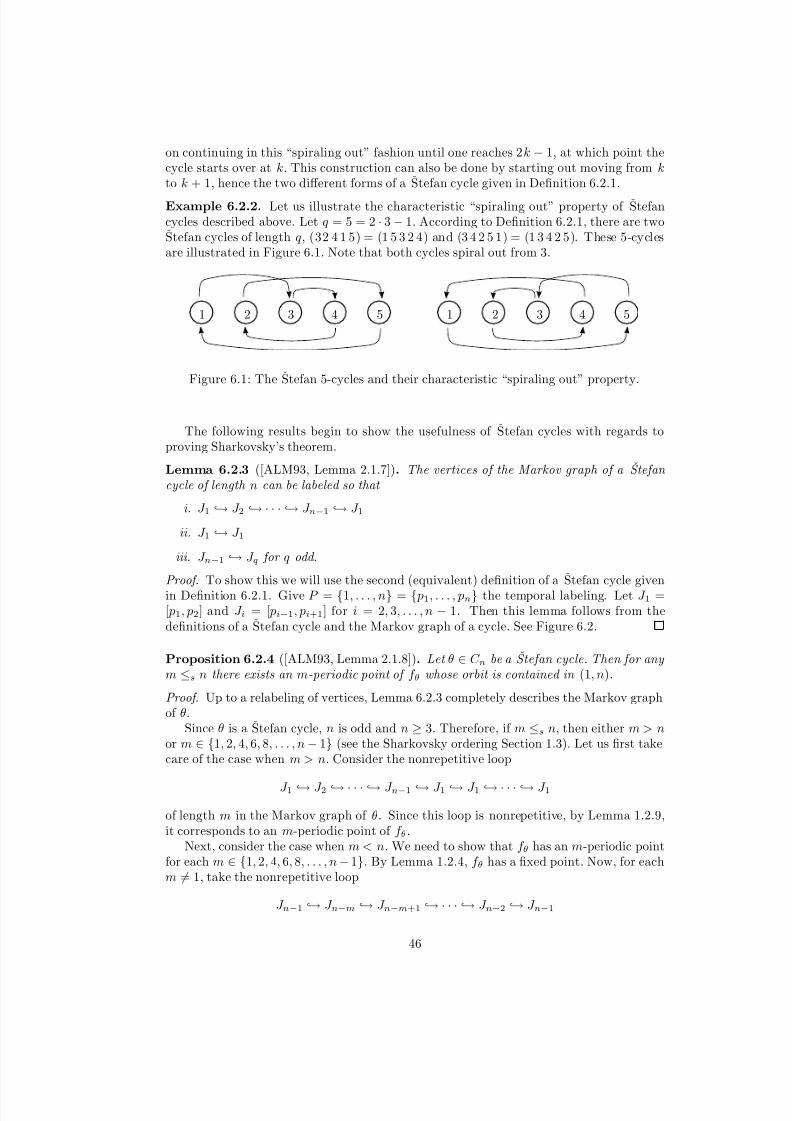
8/3/2019 Thesis 4-26-09


on continuing in this “spiraling out” fashion until one reaches 2k − 1, at which point thecycle starts over at k. This construction can also be done by starting out moving from kto k + 1, hence the two different forms of a Stefan cycle given in Definition 6.2.1.

Example 6.2.2. Let us illustrate the characteristic “spiraling out” property of Stefancycles described above. Let q = 5 = 2 · 3 − 1. According to Definition 6.2.1, there are twoStefan cycles of length q, (32 4 1 5) = (1 5 3 2 4) and (3 4 2 5 1) = (1 3 4 2 5). These 5-cyclesare illustrated in Figure 6.1. Note that both cycles spiral out from 3.

1 2 3 4 5 1 2 3 4 5

Figure 6.1: The Stefan 5-cycles and their characteristic “spiraling out” property.

The following results begin to show the usefulness of Stefan cycles with regards toproving Sharkovsky’s theorem.

Lemma 6.2.3 ([ALM93, Lemma 2.1.7]). The vertices of the Markov graph of a ˇ Stefan cycle of length n can be labeled so that

i. J 1 → J 2 → · · · → J n−1 → J 1

ii. J 1 → J 1

iii. J n−1 → J q for q odd.

Proof. To show this we will use the second (equivalent) definition of a Stefan cycle givenin Definition 6.2.1. Give P = {1, . . . , n} = { p1, . . . , pn} the temporal labeling. Let J 1 =[ p1, p2] and J i = [ pi−1, pi+1] for i = 2, 3, . . . , n − 1. Then this lemma follows from thedefinitions of a Stefan cycle and the Markov graph of a cycle. See Figure 6.2.

Proposition 6.2.4 ([ALM93, Lemma 2.1.8]). Let θ ∈ C n be a ˇ Stefan cycle. Then for any m ≤s n there exists an m-periodic point of f θ whose orbit is contained in (1, n).

Proof. Up to a relabeling of vertices, Lemma 6.2.3 completely describes the Markov graphof θ.

Since θ is a Stefan cycle, n is odd and n ≥ 3. Therefore, if m ≤s n, then either m > nor m ∈ {1, 2, 4, 6, 8, . . . , n − 1} (see the Sharkovsky ordering Section 1.3). Let us first takecare of the case when m > n. Consider the nonrepetitive loop

J 1 → J 2 → · · · → J n−1 → J 1 → J 1 → · · · → J 1

of length m in the Markov graph of θ. Since this loop is nonrepetitive, by Lemma 1.2.9,it corresponds to an m-periodic point of f θ.

Next, consider the case when m < n. We need to show that f θ has an m-periodic pointfor each m ∈ {1, 2, 4, 6, 8, . . . , n − 1}. By Lemma 1.2.4, f θ has a fixed point. Now, for eachm = 1, take the nonrepetitive loop

J n−1 → J n−m → J n−m+1 → · · · → J n−2 → J n−1

46

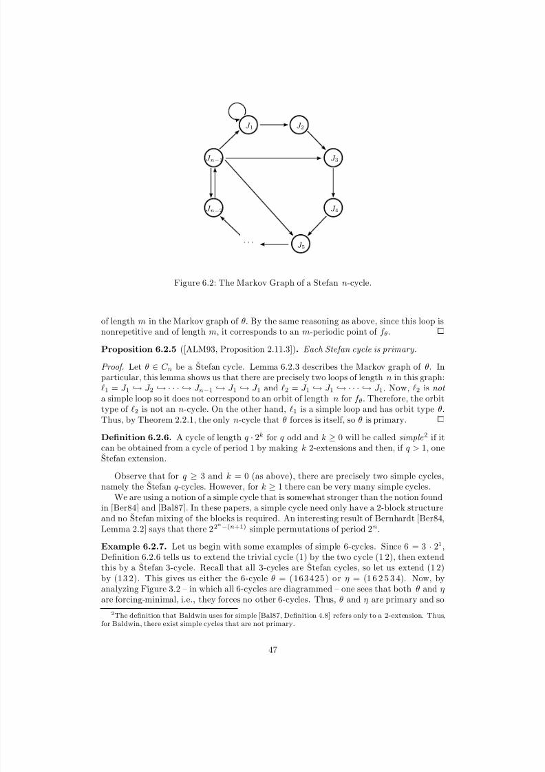
8/3/2019 Thesis 4-26-09


J 1 J 2

J n−1 J 3

J n−2 J 4

· · · J 5

Figure 6.2: The Markov Graph of a Stefan n-cycle.

of length m in the Markov graph of θ. By the same reasoning as above, since this loop isnonrepetitive and of length m, it corresponds to an m-periodic point of f θ.

Proposition 6.2.5 ([ALM93, Proposition 2.11.3]). Each Stefan cycle is primary.

Proof. Let θ ∈ C n be a Stefan cycle. Lemma 6.2.3 describes the Markov graph of θ. Inparticular, this lemma shows us that there are precisely two loops of length n in this graph:1 = J 1 → J 2 → · · · → J n−1 → J 1 → J 1 and 2 = J 1 → J 1 → · · · → J 1. Now, 2 is not a simple loop so it does not correspond to an orbit of length n for f θ. Therefore, the orbit

type of 2 is not an n-cycle. On the other hand, 1 is a simple loop and has orbit type θ.Thus, by Theorem 2.2.1, the only n-cycle that θ forces is itself, so θ is primary.

Definition 6.2.6. A cycle of length q · 2k for q odd and k ≥ 0 will be called simple2 if itcan be obtained from a cycle of period 1 by making k 2-extensions and then, if q > 1, oneStefan extension.

Observe that for q ≥ 3 and k = 0 (as above), there are precisely two simple cycles,namely the Stefan q-cycles. However, for k ≥ 1 there can be very many simple cycles.

We are using a notion of a simple cycle that is somewhat stronger than the notion foundin [Ber84] and [Bal87]. In these papers, a simple cycle need only have a 2-block structureand no Stefan mixing of the blocks is required. An interesting result of Bernhardt [Ber84,Lemma 2.2] says that there 22n−(n+1) simple permutations of period 2n.

Example 6.2.7. Let us begin with some examples of simple 6-cycles. Since 6 = 3 · 21,Definition 6.2.6 tells us to extend the trivial cycle (1) by the two cycle (1 2), then extendthis by a Stefan 3-cycle. Recall that all 3-cycles are Stefan cycles, so let us extend (1 2)by (1 3 2). This gives us either the 6-cycle θ = ( 163425) or η = (1 6 2 5 3 4). Now, byanalyzing Figure 3.2 – in which all 6-cycles are diagrammed – one sees that both θ and ηare forcing-minimal, i.e., they forces no other 6-cycles. Thus, θ and η are primary and so

2The definition that Baldwin uses for simple [Bal87, Definition 4.8] refers only to a 2-extension. Thus,for Baldwin, there exist simple cycles that are not primary.

47

8/3/2019 Thesis 4-26-09


by Proposition 6.1.2, θ = (1 4 3 5 2 6) and η = (15 2 4 3 6) should also be primary. Looking

again at Figure 3.2, we see that indeed θ and η are primary. Lastly, we note that had wechosen to extend (1 2) by (1 2 3) instead of (1 3 2), we would have have produced θ and η.

Consequently, the above discussion gives all of the primary and simple 6-cycles. Figure6.3 illustrates the fact that all of the simple 6-cycles have the characteristic “two block”and “spiraling Stefan ” structure.

1 2 3 4 5 6 1 2 3 4 5 6

1 2 3 4 5 6 1 2 3 4 5 6

θ = (16 34 25) η = (16 25 34)

θ = (1 4 3 5 2 6) η = (15 24 36)

Figure 6.3: The primary and simple 6-cycles.

Example 6.2.7 points towards the most important theorem of this section, namely

Theorem 6.2.10, which says a cycle is primary if and only if it is simple. This will beone of the keys to proving Sharkovsky’s theorem via forcing. We will first work towardsshowing that simple ⇒ primary. To do so, wee need a couple of lemmas. The first lemma,Lemma 6.2.8, essentially tells us that the simple cycles of length 2 k form a tree in theforcing relation. The second lemma, Lemma 6.2.9, shows that any primary extension of asimple cycle of length a power of 2 is itself primary.

Lemma 6.2.8 ([ALM93, Lemma 2.11.5]). Let θ be a simple cycle of length 2k for somek ≥ 0. If θ forces η, then η is a 2j-cycle for some j ≤ k such that η ∈ C 2j .

Proof. This result follows almost immediately from the section on doublings (Section 5.1).We prove this by induction on k. For k = 0, the result is trivial. Now, assume that theresult holds for simple cycles of length 2k−1. If θ is a simple 2k-cycle, then θ is a doubling

of a simple cycle of length 2k−1

. Therefore, if θ forces η, then by Lemma 5.2.10 andthe inductive hypothesis, we must have either η is a 2k-cycle or η is a 2j-cycle for some

j ≤ k − 1.

Lemma 6.2.9 ([ALM93, Lemma 2.11.6]). Let η be a simple 2k-cycle for some k ≥ 0. If θ is a nontrivial extension of η, then θ is primary.

Proof. The restriction that θ is not an extension guarantees that the length of θ is strictlygreater than the length of η. Now, from the previous lemma, Lemma 6.2.8, it follows that

48

8/3/2019 Thesis 4-26-09


η does not force any cycle of length larger than 2k. By Corollary 6.1.4, we conclude thatθ is indeed primary.

Theorem 6.2.10 ([ALM93, Theorem 2.11.7]). A cycle is primary if and only if it issimple.

Proof that simple implies primary. Let θ be a simple cycle. First, if θ is of odd length,say q ≥ 3, then θ is a Stefan cycle. By Proposition 6.2.5, θ is primary. Next, supposethat θ is of length 2k for k ≥ 0. As remarked after the definition of primarity, if k = 0or k = 1 then θ must be primary. If, however, k > 1, then since (1 2) is primary, takingthe contrapositive of Lemma 6.2.9, we see that θ is primary. Lastly, suppose that θ is of length q · 2k with q ≥ 3 odd. Then, combining both Lemma 6.2.9 and Proposition 6.2.5,we get that θ is primary.

To prove the reverse direction that a primary cycle is simple requires a considerableamount of work that would amount to reproducing [BC86] or several sections of [ALM93].Therefore, we will try to give a detailed sketch of how one shows that primary impliessimple.

Let us first show how Alseda, LLibre and Misiurewicz proved the result in [ALM93].First, they show that depending on the length of a cycle, a primary cycle is either a Stefancycle or has a block structure over (1 2).

Proposition 6.2.11 ([ALM93, Proposition 2.11.8]). Let θ be a nontrivial primary cycle.Then the following statements hold.

(a) If |θ| is even, then θ has a block structure over (12).

(b) If |θ| is odd, then θ is a ˇ Stefan cycle.

The proof of this proposition requires the result that given any n-cycle θ, there existsan interval map f such that f has an n-periodic point x, f is O(x)-monotone and O(x)

is the unique orbit of f that exhibits θ [ALM93, Proposition 2.5.4]. This can be provenby using the “pouring water” construction [ALM93, p. 54]. Observe that this result isalmost guaranteed by the doubling theorem (Theorem 5.1.6) which says that so long as θis not a doubling, P = {1, 2, . . . , n} is the unique invariant set of f θ that exhibits θ.

Now, as an immediate consequence of Proposition 6.2.11 we have that for nontrivialodd-lengthed cycles, primary implies simple. This is because given an odd-length primarycycle θ, Proposition 6.2.11 implies θ is a Stefan cycle, and by the definition of a simple cycle,a Stefan cycle is simple. What remains to be shown is that any even-lengthed primarycycle (which by Proposition 6.2.11 has a block structure over (1 2)) is in fact a simple cycle.To do so, requires very careful analysis of these block structures. Ultimately, one showsthat for a primary even-lengthed cycle θ, the first-return patterns of the blocks are Stefancycles of the same length and so θ is a Stefan extension of some cycle [ALM93, Lemmas2.11.9 - 2.11.16]. Moreover, they show that if θ is a primary n · 2k-cycle, then θ has a blockstructure over a simple 2k-cycle [ALM93, Proposition 2.11.17].

Block and Coppel [BC86] and Baldwin [Bal87, Theorem 4.9] (which heavily uses Blockand Coppel’s paper) proved the result that primary implies simple in a slightly differentway. Block and Coppel prove the following powerful theorem which essentially completesthe proof:

Theorem 6.2.12 ([BC86, Theorem 1]). If f has an orbit of period n, then it has a (strongly) simple orbit of period n.

49

8/3/2019 Thesis 4-26-09


Now, suppose that θ is a primary cycle. By Theorem 6.2.12, f θ exhibits a simple cycle,say η, of period n and so by the Forcing Theorem, θ→η. But, since θ is primary, i.e.forcing-minimal, it forces no other distinct n-cycles and so we must have θ = η; that is θ

is simple. Thus, primary implies simple.We end this chapter with a diagram of all primary cycles of length ≤ 8 (Figure 6.4).

Again, recall that θ forces η in this diagram if and only if θ is above η and there is a linesegment from θ to η. For example, in Figure 6.4 we see that (1 2 3) forces (1 3 4 2 5), but(1 2 3) does not force (1 7 4 3 5 2 6) . To find all primary cycles of length less than or equalto 8, we modified the algorithm from Chapter 3 as illustrated by the following pseudocode:

primaryCycles := [];

for k in {3,...,8} do

if k odd then

Append(primaryCycles,stefanCycles(k));

else

G:=cyclicPermutations(SymmetricGroup(k));

for g in G doif g has a 2-block structure then

if the set of k-cycles forced by g is empty then

Append(primaryCycles,g);

return primaryCycles;

Earlier, it was stated that there are 22n−(n+1) cycles of length 2n that have a 2-block struc-ture. Thus, this algorithm clearly becomes inefficient for k even, k ≥ 10, but neverthelessdoes the job for k ≤ 8.

50

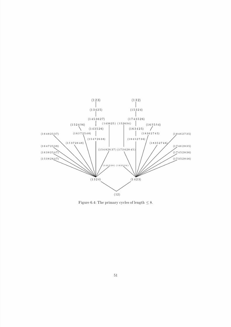
8/3/2019 Thesis 4-26-09


8/3/2019 Thesis 4-26-09


Chapter 7

A Forcing Proof of

Sharkovsky’s Theorem

We will now prove Sharkovsky’s theorem (Theorem 1.3.1) by employing the various resultsabout the local, global and minimality properties of forcing elucidated in earlier chapters.The forcing proof of Sharkovsky’s theorem that we will present first appeared in [ALM89],but the form which we give more closely follows [ALM93, Second proof of Theorem 2.1.5].

Proof of Sharkovsky’s theorem. We aim to show that if an interval map f has an n-periodicpoint and m ≤s n then f has periodic point of period m. If n = 1 then there is nothing toprove. So, let us assume that that n ≥ 2. Let P denote the orbit of our n-periodic point,and let θ be the n-cycle that P exhibits. The first key point to note is that Proposition6.1.3 allows us to assume that θ is primary because there exists a primary n-cycle that θforces. Moreover, in view of Theorem 6.2.10, we may also assume that θ is simple.

Now, suppose that n is odd. Since every odd-lengthed simple cycle is aˇStefan cycle, θis a Stefan cycle. But, since θ is a Stefan cycle, the result follows from Proposition 6.2.4

which shows that the Markov graph of θ has a nonrepetitive loop of length m for everym ≤s n.

Next, suppose that n is a power of 2. Then, the statement follows from the definitionof a simple cycle and the inductive use of Corollary 5.2.4. Therefore, we are left withthe case n = q · 2k with k > 0 and q ≥ 3 odd. In this case, m ≤s n implies that eitherm = r · 2k with r ≤s q or m = 2i and i < k .

Since θ is simple, by Defintion 6.2.6, it is a τ -extension of a simple cycle η of period2k where τ is one of the two Stefan cycles of length q. (We will see that the choice of τ does not matter). Let us first assume that m = r · 2k and r ≤s q. By Lemma 6.2.4 andProposition 6.1.3, τ forces some cycle π of period r. Then by Lemma 5.2.11, θ forces someπ-extension of η. This π-extension of η has period m and hence f has a cycle of period

m. Assume now that m = 2i

with i < k. By Corollary 5.2.4, we get θ→η. Again by theinductive use of Corollary 5.2.4 we get that η forces some cycle η of period m. Then θ→ηand f has a cycle of period m. This completes the proof.

52

8/3/2019 Thesis 4-26-09


Chapter 8

Conclusions

In this chapter, we reflect on different ways in which the theory presented can be gener-

alized. To begin with, we have chosen to develop the theory of forcing from the point of view of oriented cycles; that is we consider the cycles θ and θ as distinct cycles (so long

as θ = θ). However, as many of the proofs intimated, the theory of forcing can also bedeveloped by considering two n-cycles θ and η equivalent if there exists a homeomorphismh : [1, n] → [1, n] such that f θ ◦ h = h ◦ f η. This is an equivalence relation, call it ∼ and

the elements of C/ ∼ are called patterns. Note that θ ∼ θ. In fact, many of the theoremswe have proven hold for patterns as well. For example, Proposition 4.1.4 is now trivial.Some results like Proposition 5.2.8 are more easily stated in terms of patterns: if we extenda cycle by θ, then the first-return pattern of any block is the pattern of θ. In the proof of Proposition 5.2.11, two different cases were required, one for when the first-return patternwas θ and one when the first-return pattern was θ. This would have been taken care of in one case by considering only the pattern of θ. Essentially, considering only patterns

amounts to cutting Figure 3.2 in half and only considering one side.In Chapter 2, the combinatorial data that we considered was the way in which thepoints of a periodic orbit were permuted. This restricted our study of forcing to cyclicpermutations only. However, in [MN91], Misiurewicz and Nitecki consider general finiteinvariant sets which allows the study of permutations as well as cycles. They prove a“combinatorial shadowing theorem”, that describes the forcing of cycles which behaveas extensions of a given one for sufficiently long time [ALM93]. This allows much moregenerality than the results that we have presented.

While this paper has addressed specifically the case of a forcing relation for one-dimensional maps, much more recent work has focused on forcing relations in higherdimensional dynamical systems. Forcing relations provide information about when thepresence of certain dynamical features, such as the existence of periodic orbits of a particu-lar type, imply the presence of other dynamical features [dCH89]. “In the one-dimensional

case, we used the period and the induced permutation as specifications of a periodic orbit:what will take their place in two dimensions? A moment’s thought is enough to convince usthat the period alone is not a useful specification: given any set of positive integers whichincludes 1, we can construct a diffeomorphism f : D2 → D2 having precisely this collectionof periods for its orbits” [Hal90]. The two-dimensional analogue of the Sharkovsky orderon periods for maps of the interval restricts to a partial order on essential pseudo-Anosovconjugacy classes in the mapping class group of the n-times punctured disk [Han97].For more information on this theory, the reader is directed to [Hal91], [dCH89], [Hal90]

53

8/3/2019 Thesis 4-26-09


and [Han97].

54

8/3/2019 Thesis 4-26-09


Bibliography

[ALM89] Lluıs Alseda, Jaume Llibre, and Michal Misiurewicz, Periodic orbits of mapsof Y , Trans. Amer. Math. Soc. 313 (1989), no. 2, 475–538. MR MR958882(90c:58145)

[ALM93] , Combinatorial dynamics and entropy in dimension one, Advanced

Series in Nonlinear Dynamics, vol. 5, World Scientific Publishing Co. Inc.,River Edge, NJ, 1993. MR MR1255515 (95j:58042)

[Bal87] Stewart Baldwin, Generalizations of a theorem of Sarkovskii on orbits of con-tinuous real-valued functions, Discrete Math. 67 (1987), no. 2, 111–127. MRMR913178 (89c:58057)

[BB04] Karen M. Brucks and Henk Bruin, Topics from one-dimensional dynamics,London Mathematical Society Student Texts, vol. 62, Cambridge UniversityPress, Cambridge, 2004. MR MR2080037 (2005j:37048)

[BC86] L. S. Block and W. A. Coppel, Stratification of continuous maps of an in-terval , Trans. Amer. Math. Soc. 297 (1986), no. 2, 587–604. MR MR854086(88a:58164)

[BC92a] Chris Bernhardt and Ethan M. Coven, A polynomial-time algorithm for de-ciding the forcing relation on cyclic permutations, Symbolic dynamics and itsapplications (New Haven, CT, 1991), Contemp. Math., vol. 135, Amer. Math.Soc., Providence, RI, 1992, pp. 85–93. MR MR1185081 (93j:58041)

[BC92b] L. S. Block and W. A. Coppel, Dynamics in one dimension , Lecture Notesin Mathematics, vol. 1513, Springer-Verlag, Berlin, 1992. MR MR1176513(93g:58091)

[BCMM92] C. Bernhardt, E. Coven, M. Misiurewicz, and I. Mulvey, Comparing periodicorbits of maps of the interval , Trans. Amer. Math. Soc. 333 (1992), no. 2,701–707. MR MR1079051 (92m:58106)

[Ber84] Chris Bernhardt, Simple permutations with order a power of two, ErgodicTheory Dynam. Systems 4 (1984), no. 2, 179–186. MR MR766099 (86d:58092)

[Ber87] , The ordering on permutations induced by continuous maps of thereal line, Ergodic Theory Dynam. Systems 7 (1987), no. 2, 155–160. MRMR896787 (88h:58099)

[BGMY80] Louis Block, John Guckenheimer, Michal Misiurewicz, and Lai Sang Young,Periodic points and topological entropy of one-dimensional maps, Global

55

8/3/2019 Thesis 4-26-09


theory of dynamical systems (Proc. Internat. Conf., Northwestern Univ.,Evanston, Ill., 1979), Lecture Notes in Math., vol. 819, Springer, Berlin, 1980,pp. 18–34. MR MR591173 (82j:58097)

[BH] Keith Burns and Boris Hasselblatt, The sharkovsky theorem: A natural direct proof , Amer. Math. Monthly ?? (??), no. ?, ?

[BS02] Michael Brin and Garrett Stuck, Introduction to dynamical systems, Cam-bridge University Press, Cambridge, 2002. MR MR1963683 (2003m:37001)

[CE80] Pierre Collet and Jean-Pierre Eckmann, Iterated maps on the interval as dy-namical systems, Progress in Physics, vol. 1, Birkhauser Boston, Mass., 1980.MR MR613981 (82j:58078)

[dCH89] Andre de Carvalho and Toby Hall, Decoration invariants for horseshoe braids,arXiv:0808.3078v1 (1989), 1–42.

[dMvS93] Welington de Melo and Sebastian van Strien, One-dimensional dynamics,Ergebnisse der Mathematik und ihrer Grenzgebiete (3) [Results in Mathe-matics and Related Areas (3)], vol. 25, Springer-Verlag, Berlin, 1993. MRMR1239171 (95a:58035)

[Hal90] Toby D. H. Hall, Coexistence theorems for periodic orbits of horseshoe type,An essay submitted in competition for the Smith prise in mathematics (1990),1–46.

[Hal91] Toby Hall, Unremovable periodic orbits of homeomorphisms, Math. Proc.Cambridge Philos. Soc. 110 (1991), no. 3, 523–531. MR MR1120486(92i:58146)

[Han97] Michael Handel, The forcing partial order on the three times punctured disk ,

Ergodic Theory Dynam. Systems 17 (1997), no. 3, 593–610. MR MR1452182(98i:57026)

[Jun91] Irwin Jungreis, Some results on the ˇ Sarkovskiı partial ordering of permuta-tions, Trans. Amer. Math. Soc. 325 (1991), no. 1, 319–344. MR MR998354(91h:58060)

[LY75] Tien Yien Li and James A. Yorke, Period three implies chaos, Amer. Math.Monthly 82 (1975), no. 10, 985–992. MR MR0385028 (52 #5898)

[Mis97] Michal Misiurewicz, Remarks on Sharkovsky’s theorem , Amer. Math. Monthly104 (1997), no. 9, 846–847. MR MR1479989 (98f:58138)

[MN91] Michal Misiurewicz and Zbigniew Nitecki, Combinatorial patterns for mapsof the interval , Mem. Amer. Math. Soc. 94 (1991), no. 456, vi+112. MRMR1086562 (92h:58105)

[MSS73] N. Metropolis, M. L. Stein, and P. R. Stein, On finite limit sets for trans- formations on the unit interval , J. Combinatorial Theory Ser. A 15 (1973),25–44. MR MR0316636 (47 #5183)

[MT88] John Milnor and William Thurston, On iterated maps of the interval , Dynam-ical systems (College Park, MD, 1986–87), Lecture Notes in Math., vol. 1342,Springer, Berlin, 1988, pp. 465–563. MR MR970571 (90a:58083)

56

8/3/2019 Thesis 4-26-09


[Nit82] Zbigniew Nitecki, Topological dynamics on the interval , Ergodic theory anddynamical systems, II (College Park, Md., 1979/1980), Progr. Math., vol. 21,Birkhauser Boston, Mass., 1982, pp. 1–73. MR MR670074 (84g:54051)

[Sha64] A. N. Sharkovsky, Co-existence of the cycles of a continuous mapping of theline into itself , Ukrain. Math. Zh. 16 (1964), no. 1, 61–71.

[Sha65] , On cycles and structure of a continuous map, Ukrain. Math. Zh. 17

(1965), no. 3, 104–111.

[Ste77] P. Stefan, A theorem of ˇ Sarkovskii on the existence of periodic orbits of con-tinuous endomorphisms of the real line, Comm. Math. Phys. 54 (1977), no. 3,237–248. MR MR0445556 (56 #3894)

[WR87] A. Weiss and T. D. Rogers, The number of orientation reversing cycles in the quadratic map, Oscillations, bifurcation and chaos (Toronto, Ont., 1986),CMS Conf. Proc., vol. 8, Amer. Math. Soc., Providence, RI, 1987, pp. 703–

711. MR MR909946 (89b:58174)

Thesis 4-26-09

Documents

Transcript of Thesis 4-26-09