The Role of Education in Development∗

Juan Carlos Córdoba†

and

Marla Ripoll‡

First Version: September 2006This Version: February 2007

Abstract

Most education around the globe is public. Moreover, investment rates in education as well asschooling attainment differ substantially across countries. We contruct a general equilibriumlife-cycle model that is consistent with these facts. We provide simple analytical solutions forthe optimal educational choices, which may entail pure public provision of education, and theirgeneral equilibrium effects. We calibrate the model to fit cross-country differences in demo-graphic and educational variables. The model is able to replicate a number of key regularitiesin the data beyond the matching targets. We use the model to identify and quantify sourcesof world income differences, and find that demographic factors, in particular mortality rates,explain most of the differences. We also use the model to study the role of public education,and the effects of the HIV/AIDS pandemic in development.

Keywords: schooling, life expectancy, mortality rates, cross-country income differences.JEL Classification: I22, J24, O11.

∗We thank Mark Bils, Daniele Coen-Pirani, David N. DeJong, Pohan Fong, Paul Gomme, Tatiana Koreshkovaand participants in seminars at the University of Rochester, Concordia University, and University of Delaware fortheir valuable comments.

†Department of Economics, Rice University, 6100 Main Street, Houston TX 77005, e-mail: jcordoba@rice.edu.‡Department of Economics, University of Pittsburgh, 4907 W.W. Posvar Hall, Pittsburgh PA 15260, e-mail:

ripoll@pitt.edu.

1 Introduction

The provision of education around the world has three salient features. First, public education

is the predominant form of education. It accounts on average for 85% and 78% of primary and

secondary enrollment respectively, a fact illustrated in Figure 1 for a set of 91 countries. Second,

richer countries invest significantly more resources in education per pupil than poor countries. For

example, the US invests 200 times more resources per pupil a year than the average of the 5 poorest

countries in our sample. Figure 2 illustrates an aspect of this fact. It portrays the investment rate

in education, defined as the ratio of public expenditures in education per pupil to per-capita GDP,

against per-capita GDP. This investment rate differs substantially across countries and increases

with income. The third feature is well-known: schooling attainment also increases with income and

differs substantially across countries (Barro and Lee, 2000).

The purpose of this paper is to construct a general equilibrium model of education and human

capital accumulation that is consistent with the set of facts mentioned above. In particular, we

study the role public education and investments in education, as well as years of schooling, in the

formation of human capital and in the wealth of nations. Our analysis has two main distinctive

features. First, in our model young individuals face credit market frictions and the government

alleviates them by providing public education. This is a departure from the frictionless Ben-Porath

model that has been the focus of recent research on human capital formation, including Manuelli

and Seshadri (MS, 2005), Hendricks (2005), and Hugget, Ventura and Yaron (2006), among others.

Second, we calibrate the key parameters of the human capital production function by targeting

moments of the cross-country distribution of schooling and returns to schooling. Competing papers

instead only employ U.S. evidence to calibrate key parameters. Thus, our calibration strategy

avoids issues that arise due to the special nature of the U.S. educational system.

We devise a simple model that incorporates key features of the data regarding education, saving

rates, life expectancy, and mortality rates, and yet has simple closed-form solutions. This allows

us to identify the mechanisms at work and properly quantify the contribution of different fun-

damentals, such as TFP, public education expenditures, mortality rates and taxes in explaining

1

income differences across countries. We show that the model performs well in other dimensions

beyond the matching targets. For example, although we only target the average return to schooling

in the calibration, the model replicates the overall distribution of returns better than alternative

well-known models. Also, our model replicates the prevalence of public education around the world

even though private education is also available in the model. Overall, we conclude that our model

provides a plausible quantitative theory of schooling, human capital, and incomes.

We then employ the model for several purposes. First, we construct human capital stocks for a

set of 91 countries and compare the results to existing alternatives. We find that our estimates are

more disperse and significantly lower for poor countries than the ones estimated using Mincer style

equations. The reason is that Mincer equations abstract from expenditures in education while our

human capital production function includes both years of schooling and expenditures as inputs.

Since public expenditures per pupil are positively correlated with per capita income, including

differences in education expenditures across countries makes human capital much lower in poorer

countries. These findings are qualitatively similar to those of MS and EKR, and quantitatively close

to those of Córdoba and Ripoll (CR, 2004), who use a completely different methodology based on

country specific rural-urban wage gaps to estimate human capitals. Finally, our human capital

estimates are different from Hendricks (2002) who finds relative minor differences in human capital

across countries using earnings of immigrants in the US. However, we show that both estimates

can be reconciled if immigrants are positively self-selected to some minor extent.

Second, we assess the sources of cross-country income differences according to the model. As

part of this assessment, we compute the long-run elasticity of output to TFP. As argued by MS, this

elasticity increases substantially in models with endogenous human capital and implies that given

TFP differences result in larger income differences. We find an elasticity of 2.4 in our model which

is substantially lower than the one found by MS of 9. On the other hand, our estimate is close to

the 2.8 value found by Erosa, Koreshkova and Restuccia (EKR, 2006) using a different model. Our

estimate implies that smaller but still important TFP differences are required to explain income

differences across countries compared to models of exogenous human capital. In contrast, MS’ large

2

elasticity implies that no TFP differences are required to explain income differences.1

A simple variance decomposition exercise shows that the role of TFP in explaining steady state

income differences decreases significantly compared to models with exogenous human capital, from

60% to 38%. In addition, counterfactual exercises show that eliminating TFP differences would

reduce the world variance of log incomes by 48%, while eliminating differences in mortality rates

would reduce this variance by 51%. Finally, eliminating differences in the provision of public

education would do so by 18%. We thus find that TFP still plays a major role in explaining income

differences, but that mortality differences are at least as important. This finding prompted us to use

the model in order to assess the effects of the HIV/AIDS pandemic on long run development. This

pandemic has increased mortality rates dramatically particularly in Sub-Saharan Africa. Contrary

to some claims in the literature, we find that the long run consequences of the pandemic are

devastating for development. For example, the model predicts that if rates of infection persist at

the current levels, the log variance of income would increase in 28%.

Our paper is related to the recent quantitative work by MS and EKR regarding human capital

differences across countries using microfounded models of human capital formation. The first

paper derives the implication of a frictionless Ben-Porath model for human capital differences,

while the second builds upon a heterogenous agent model in the Bewley tradition. MS consider

pure private education, a feature inconsistent with Figure 1. Our model is similar to MS in its

use of a representative agent model and its treatment of demographic factors, but we focus on the

role of public education and credit market frictions in the formation of human capital, and our

calibration strategy is very different. While MS calibrate the key parameters of the human capital

technology to match life-cycle earning in the US, we calibrate these parameters to match features

of the cross-country distribution of schooling and returns to schooling. We arrive to substantially

different quantitative results.

On the other hand, our model is similar to EKR in the treatment of public education and in

some aggregate results. The models, however, are very different. In their model, TFP is the only1This comparisson is between the complete models that include, among others things, variation in demographics

and in the price of capital.

3

source of variation explaining income and schooling differences, while mortality rates, as well as

TFP, play the key role in our model. EKR do not consider the role of mortality rates in generating

differences in human capital accumulation across countries. In contrast, MS, Bils and Klenow (2000)

and Ferreira and Pessoa (2003) find, as we do, that these differences in mortality are important.

Finally, EKR calibrate their model to match moments of the cross sectional distribution of earnings

and schooling in the US, while we target the cross-country distribution of schooling and returns.

Finally, in our model permanent TFP differences do not affect years of schooling while they

do in MS and EKR. This feature of their models provides an additional channel for TFP to affect

income. However, it also implies that their models do not possess a balanced growth path, while

ours does. To the extent that a balanced growth path is regarded as a desirable property of a

growth model, our model provides a plausible theory of human capital and income differences. A

further advantage of our modeling approach is that we are able to obtain closed-form solutions for

most of our results.

The remaining of the paper is organized as follows. Section 2 lays down the model. Section 3

calibrates it and provides overidentifying tests. Section 4 reports human capital estimates. Section

5 presents the implications of the model for cross-country income differences as well as some coun-

terfactual exercises. Section 6 reports the results for HIV/AIDS pandemic. Section 7 concludes.

2 The Model

Consider an economy composed of I generations of individuals, competitive firms hiring labor and

renting capital to produce finals goods, and competitive mutual funds managing individuals savings

and the capital stock of the economy. Denote Ni, for i = {1, .., I}, the population size of generation

i, and N the total population. Schooling-age individuals (i = 1), or “children” for short, can work

or go to school while adults (i = {2, ..., I}) only work.2 A period in the model last for T years, and

individuals live for a maximum of I · T years.2 In the calibration below, “children” are individuals between the ages of 6 to 26 years.

4

Demographics Of any given cohort only a fraction πi survive to age i. We define π1 = 1 and

πI+1 = 0. Life expectancy at birth is given by T ·PIi=1 πi. The population size of children satisfy

N1 = fN2, where f is the fertility rate of young adults (i = 2). Only young adults have children.

We focus on a steady state demographic situation in which total population is growing at a constant

rate. Since N01 = fN

02 = fπ2N1, where (

0) denotes next period, then the common growth rate for

all groups along a steady state is:N 0

N= fπ2. (1)

Moreover, in steady state the age composition of the population is stable and described by (see

details in the Appendix):

ni ≡NiN=

πi · (fπ2)−iPIj=1 πj · (fπ2)

−j . (2)

The Production of Human Capital Children’s human capital, h1, is assumed to be a fraction

θ1 of the average parental human capital, hp. Young adults’ human capital, h2, depends on human

capital investments undertaken during childhood:

h2 = z (χ+ s)γ1 xγ2 (3)

where [z, γ1, γ2] > 0 are technological parameters, χ are pre-school years, s are years of formal

schooling, x are educational expenditures in the form of final goods. Human capital for later

periods of life are assumed to be a proportion θi ≥ 0, i ∈ {3, .., I}, of h2. Thus, human capital

investments during childhood determine the whole path of human capitals during the individual’s

life. The parameters θi allow to capture the life-cycle profile of earnings while h2 determines its level.

For example, θi = 1 represents a flat life-cycle earning profile at the level h2. For completeness,

define θ2 ≡ 1.

5

Individuals’ Problem Individuals maximize their lifetime welfare as described by:

IXi=1

πiρi−1 ln ci

where ci is consumption at age i, and ρ is a discount factor. Moreover, individuals face the following

resource and technological restrictions during their life time:

wh1(1− s/T ) = c1 + e, e ≥ 0, s ∈ [0, T ] . (4)

whi + (1 + r)ai−1 = ci + ai, a1 = aI = 0, i = 2, .., I. (5)

h1 = θ1hp, (6)

h2 = z (χ+ s)γ1 (p+ e)γ2 , (7)

hi = θih2 for i = 3, ..., I. (8)

where w = (1− τ)w is the after-tax wage, τ is a proportional tax on income, ai are savings at age

i, r is the net return on savings, e are private expenses in education, and p are public expenditures

in education per child. Individuals maximize overn{ci, ai, hi}Ii=1 , s, e,

o.

The first restriction states that the after-tax labor income during the first period of life can

be used to consume or to invest in education. In particular, children cannot borrow. Equations

in (5) are the set of budget constraints during adulthood. The remaining equation describe the

accumulation of human capital. Notice that children receive public subsidies for education, p, which

enter directly in the constraint (7).

Although parents in our life-cycle formulation are not altruistic, they do help their children in

two ways. First, they provide them with an earning potential during their schooling-age years that

is tied to their own earning potential. This is a form of “unintended” bequest that allows children

to consume and invest in education. Moreover, it implies that individuals in richer economies

can consume and invest more in education than individuals in poorer economies. Second, parents

6

also help children by financing the public education system through proportional income taxes.

This form of “social” bequest reinforces the ability of children in richer economies to afford more

consumption and investment.

Firms Output is produced by a representative competitive firm operating a Cobb-Douglas tech-

nology:

Y = AKαH1−α, 0 < α < 1,

where Y denotes output, K represent physical capital services, and H represents human capital

services. The firm hires labor and capital in competitive markets at the rates w per unit of human

capital and r per unit of capital. Profit maximization entails the following conditions:

w = (1− α)Y

H, r = α

Y

K. (9)

Mutual Funds Individuals deposit their savings in mutual funds (MFs). MFs own the capital

stock of the economy, and rent it to firms at the rate r. MFs operate a constant returns to scale

technology that transform q units of output into 1 unit of capital. Thus, q is the price of capital

in terms of final goods, the numeraire. MFs are competitive, pay proportional taxes τ on earned

income, and returns r to the surviving depositors. Without loss of generality, consider a single

MF that holds all the capital stock in the economy, K 0 =PIi=1Niai/q. Free entry guarantees zero

profits so that:

((1− δ) q + r (1− τ))K 0 = (1 + r)IXi=1

πi+1πi

Niai,

where δ is the depreciation rate of capital and πi+1/πi is the fraction of the population of age i

that reaches age i+ 1. Thus:

1 + r = (r (1− τ) /q + 1− δ)

PIi=1NiaiPI

i=1πi+1πiNiai

.

7

Note that for the case of constant survival probability, πi = πi−1, this equation becomes the more

standard expression 1 + r = (r (1− τ) /q + 1− δ) /π.

Government The government collects proportional taxes on capital and labor income to finance

government expenditures, G, that is, G = τ(wH + rK). Using (9) this equation can be written as

G = τY . Moreover, a fraction 0 < ε < 1 of G is allocated to public education: N1p = εG. Thus:

p = ετY/N1. (10)

Resource Constraints Gross output, which includes undepreciated capital, can be used for con-

sumption by all individuals (C), private education, government services, or to accumulate capital:

Y + (1− δ) qK = C +N1e+G+ qK0.

Next period capital stock, K 0, is the sum of individuals’ savings divided by q. Finally, aggregate

human capital, H, is the sum of individuals’ human capital available for production.

Definition of Equilibrium Let y = Y/N , k = K/N , and h = H/N . The following is our

definition of equilibrium:

Definition A stationary competitive equilibrium for given taxes τ are prices w and r, quantitiesn{c∗i , a∗i , h∗i }

Ii=1 , s

∗, e∗o, hp, k, y, and h, and subsidies p such that (i) given hp, prices, taxes,

and subsidies,n{c∗i , a∗i , h∗i }

Ii=1 , s

∗, e∗osolves the individual problem; (ii) given y, k and h, w

and r satisfy w = (1− τ) (1− α) y/h, 1+r =¡αyk (1− τ) /q + 1− δ

¢ ³PIi=1Nia

∗i /PIi=1

πi+1πiNia

∗i

´;

(iii) hp = h∗2, h = (1− s∗/T )n1h∗1 +P2 nih

∗i , qk =

PIi=1 nia

∗i , y = Ak

αh1−α, p = ετy/n1.

Note that in a stationary equilibrium:

h =

Ã(1− s∗/T )n1θ1 +

X2

θini

!h∗2, and (11)

8

h∗2 = z (χ+ s∗)γ1 (p+ e∗)γ2 . (12)

2.1 Characterization of the Equilibrium

Individuals’ Problem We now characterize the solution to the individuals’ problem given prices

and policies. Optimal choices may imply corner solutions. We denote “public education” the case

in which e∗ = 0 and s∗ > 0, “no formal education” the case in which s∗ = 0 and e∗ > 0, “mixed

education” the case e∗ > 0 and s∗ > 0, and “no education” the case e∗ = 0 and s∗ = 0.

The following proposition describes optimal educational choices. All proofs are in the Appendix.

First define:

eρ ≡ IXi=2

ρi−1πi; m ≡eργ2 (1 + χ/T )

1 + eργ1 ; m ≡ (1 + eργ2)χ/Teργ1 − 1

The following assumption facilitates the presentation of the results (reduces the number of cases to

present), but plays no essential role in the derivations or in the quantitative work.

Assumption 1 eργψ ≥ χ/T .

This assumption guarantees that pre-school is not too important as to make formal schooling

unattractive. It is easy to check that under Assumption 1 m > m > 0.

Proposition 1 Given prices and policies, the optimal solution for schooling years, s∗, and private

expenditures in education, e∗, are:

s∗ =

⎧⎪⎪⎪⎪⎨⎪⎪⎪⎪⎩0 for m > p

wh1eργ1T1+eρ(γ1+γ2)

hpwh1−m

ifor m ≥ p

wh1≥ m

eργ1T−χ1+eργ1 for p

wh1> m

,

e∗

wh=

⎧⎪⎪⎪⎪⎨⎪⎪⎪⎪⎩eργ2−p/wh11+eργ2 for m > p

wh1

1+eργ11+eρ(γ1+γ2)

hm− p

wh1

ifor m ≥ p

wh1≥ m

0 for pwh1

> m

.

9

Proposition 1 is illustrated in Figure 3.3 It typifies educational choices in three categories de-

pending on the ratio of pubic subsidies to potential earnings during childhood, p/(wh1). Informally,

the proposition shows that lack of public funding may prevent any formal schooling to take place,

and too much public funding may crowd-out completely private investments in education.

More formally, according to Proposition 1 the “public education” case arises when p > mwh1.

In this situation, individuals do not invest resources but only time in formal education. Since

the threshold level depends on labor income during childhood, the model predicts that poorer

individuals would be more likely to choose only public education than richer individuals. The

“mixed education” case occurs when the amount of public funding falls within an intermediate

range (m ≥ p/(wh1) ≥ m). Finally, the case of “no formal education” occurs when the public

provision of education is below certain threshold (p/(wh1) < m). In this case, insufficient funding

discourages formal schooling. Under Assumption 1, the case “no education” cannot arise.

Proposition 1 also has the following implications for the role of public education on educational

outcomes. First, additional public funding increases years of schooling only if m ≥ p/(wh1) ≥ m.

Otherwise, years of schooling do not respond to changes in public funding. An interpretation

of this result is that increasing public funding of education does not affect years of schooling of

individuals already in public schools, although it enhances their human capital. Second, private

funding responds less than one to one to changes in public funding. Specifically, |∂e/∂p| < 1

whenever e > 0. Thus, additional public funding crows out private funding but not completely,

despite public and private funding being perfect substitutes in the production function. The reason

is that public funding relaxes borrowing constraints which hinder private funding in the first place.

Proposition 1 also highlights the critical role of demographic factors in educational choices. It

states that individuals in economies with lower mortality rate, larger eρ, would choose more years ofschooling and larger private funding of education for any given size of the public sector. As we see

3A useful result to check the continuity of the choices at the threshold levels is to note that:

m−m =1 + eρψ (γ1 + γ2)

(1 + eρψγ2)eρψγ1 (eρψγ1 − χ/T ) .

10

below, this mechanism turns out to explain most of the differential in schooling across countries.

Moreover, Proposition 1 also states that z, the learning ability parameter, does not affect the

choice of schooling years or educational expenditures. Our model predicts that children do not

self-select into a pure public, private, or mixed educational regime based on their learning ability.

In particular, high ability children do not invest more years or resources in education than low

ability children.

Finally, Proposition 1 states that private funding of education depends on potential earning

levels (wh1) but years of schooling depends on the ratio of public education spending to earnings

(p/(wh1)). An important implication of this result, to be described below in detail, is that TFP

differences would induce differences in educational expenses but not in years of schooling. In this

regard, our model has different implications from the models analyzed by MS and EKR, models in

which years of schooling depend on TFP levels.

Education in General Equilibrium The following proposition characterizes the educational

choices in general equilibrium. For this purpose, the ratio p/(wh1) can be solved from equations

(10), (9) and (11) as:p

wh1=

ετ (1− s/T +P2 θini/ (θ1n1))

(1− τ) (1− α). (13)

Note that ετ is the share of public education in output (see equation 10). Substituting this result

into Proposition 1 yields Proposition 2. Proofs are in the Appendix. First define:

sH ≡(1− τ) (1− α)m

(1 + χ/T +m) / (1 + eρ) +P2 θini/ (θ1n1); sH ≡

(1− τ) (1− α)m

1 +P2 θini/ (θ1n1)

Proposition 2 The optimal solution for schooling years, s∗, and the share of educational expen-

ditures in output, s∗H , are given by:

s∗ =

⎧⎪⎪⎪⎪⎨⎪⎪⎪⎪⎩0 for sH > ετ

(ετ−sH)eργ1Tm/sH1+eρ(γ1+γ2+ετγ1/((1−τ)(1−α))) for sH ≥ ετ ≥ sHeργ1T−χ

1+eργ1 for ετ > sH

,

11

s∗H =

⎧⎪⎪⎪⎪⎨⎪⎪⎪⎪⎩ετ + (1−τ)(1−α)

1+P2 θini/(θ1n1)

eργ2−ετm/sH1+eργ2 for sH > ετ

ετ + (1−τ)(1−α)1−s∗/T+

P2 θini/(θ1n1)

(sH−ετ)(1+eργ1)m/sH1+eρ(γ1+γ2+ετγ1/((1−τ)(1−α))) for sH ≥ ετ ≥ sH

ετ for ετ > sH

.

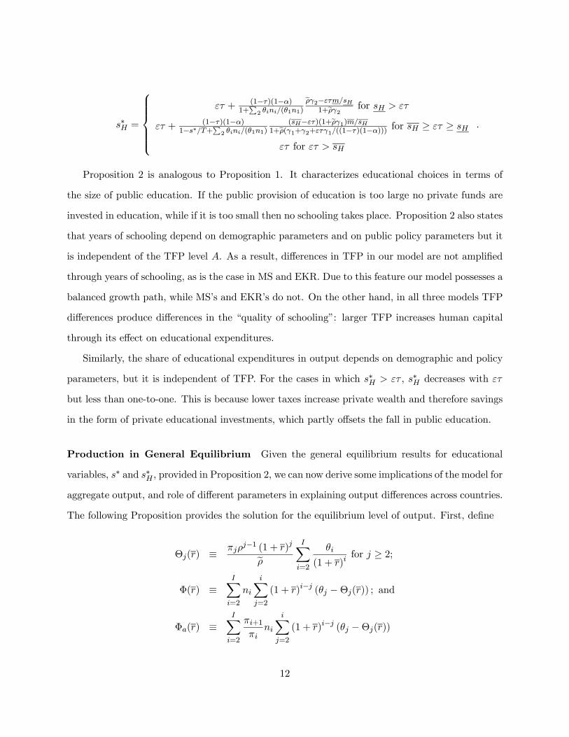
Proposition 2 is analogous to Proposition 1. It characterizes educational choices in terms of

the size of public education. If the public provision of education is too large no private funds are

invested in education, while if it is too small then no schooling takes place. Proposition 2 also states

that years of schooling depend on demographic parameters and on public policy parameters but it

is independent of the TFP level A. As a result, differences in TFP in our model are not amplified

through years of schooling, as is the case in MS and EKR. Due to this feature our model possesses a

balanced growth path, while MS’s and EKR’s do not. On the other hand, in all three models TFP

differences produce differences in the “quality of schooling”: larger TFP increases human capital

through its effect on educational expenditures.

Similarly, the share of educational expenditures in output depends on demographic and policy

parameters, but it is independent of TFP. For the cases in which s∗H > ετ , s∗H decreases with ετ

but less than one-to-one. This is because lower taxes increase private wealth and therefore savings

in the form of private educational investments, which partly offsets the fall in public education.

Production in General Equilibrium Given the general equilibrium results for educational

variables, s∗ and s∗H , provided in Proposition 2, we can now derive some implications of the model for

aggregate output, and role of different parameters in explaining output differences across countries.

The following Proposition provides the solution for the equilibrium level of output. First, define

Θj(r) ≡πjρ

j−1 (1 + r)jeρIXi=2

θi

(1 + r)ifor j ≥ 2;

Φ(r) ≡IXi=2

ni

iXj=2

(1 + r)i−j (θj −Θj(r)) ; and

Φa(r) ≡IXi=2

πi+1πi

ni

iXj=2

(1 + r)i−j (θj −Θj(r))

12

Proposition 3 The equilibrium level of output is given by:

y = A1

(1−α)(1−γ2)

µk

y

¶ α(1−α)(1−γ2)

µh

yγ2

¶ 11−γ2

(14)

whereh

yγ2=

Ã(1− s∗/T )n1θ1 +

X2

θini

!z (χ+ s∗)γ1 (s∗H/n1)

γ2 , (15)

k

y=

(1− α) (1− τ) /q

(1− s∗/T )n1θ1 +P2 θini

Φ(r), (16)

r =³1− δ + α (1− τ)

y

k/q´ Φ(r)Φa(r)

− 1 (17)

Equation (14) in Proposition 3 provides the determination of aggregate and per capita output

in three components. The first component, A1

(1−α)(1−γ2) = A1+ α

1−α+γ2

(1−α)(1−γ2) , collects the direct

and indirect effects of TFP on steady state output. The elasticity of output with respect to TFP,

1 + α/ (1− α) + γ2/ [(1− α) (1− γ2)], can be itself decomposed in three parts. The first part

captures the direct effect of TFP on output; the second part captures the indirect effect of TFP on

output through its effect on capital accumulation; and the third part captures the indirect effect

of TFP on output through its effect on human capital accumulation. This last effect has being

recently stressed in the works of MS and EKR and its quantitative significance depends only the

size of γ2. If γ2 = 0, then equation (14) adopts the more standard form used in the works of Hall

and Jones (HJ, 1999) and Klenow and Rodriguez-Clare (KRC, 1997), among others.

The second component collects the direct and indirect effects of the capital-output ratio in

output. According to equation (14), the elasticity of output with respect to the capital-output

ratio, α/ [(1− α) (1− γ2)], is also affected by γ2. This elasticity can be written as α/ (1− α) +

γ2/ [(1− α) (1− γ2)]. The second term captures the effect that a higher capital-output has on the

accumulation of human capital and on output.

The third component, (h/yγ2)1

1−γ2 , is related to the accumulation of human capital. In a

standard formulation with exogenous human capital (γ2 = 0), this component is just the stock of

13

human capital. If human capital is endogenous, this component captures the effect of educational

decisions, which themselves are function of demographic and policy parameters, but independent

of TFP, as shown in equation (15).

Equations (16) and (17) jointly determine the capital output ratio, k/y, and the net returns

r. Both variables depend on demographic factors (πi, ni), years of schooling s∗, and taxes τ .

Importantly, they are independent of TFP, particularly because s∗ is independent of TFP as stated

in Proposition 2. The positive dependence of k/y years schooling is due to the fact that a larger

fraction of students reduces labor supply, increases wages for all, in particular for adults, and

therefore their savings. Thus, the effect of schooling on the term k/y captures an extensive margin,

as more schooling reduces labor supply, while its effect on h/yγ2 captures an intensive margin, as

schooling increases adult’s human capital.

Mincerian Returns Psacharopoulos and Patrinos (2002) have collected Mincerian returns for

a fairly large set of countries. Matching these returns provides a natural test for any quantitative

model of schooling. Mincer returns, or simply returns to schooling, are obtained from a cross-section

of individuals in each country using a OLS regressions of the type:

ln(di) = a+ bsi + cXi + vi (18)

where di are earnings of individual i, b is known as the Mincerian return, and Xi is a vector of

controls. In order to use these estimates, we need to derive the theoretical counterpart of equation

(18) in our model. This requires to reformulate the model so that individuals in a given cohort are

heterogenous in terms of earnings and schooling. Suppose only for this section that each cohort

is composed of a cross-section of individuals that differ both in their learning ability, zi, and in

their discount parameter eρi. Yearly earnings during young adulthood, di, are given in our model

14

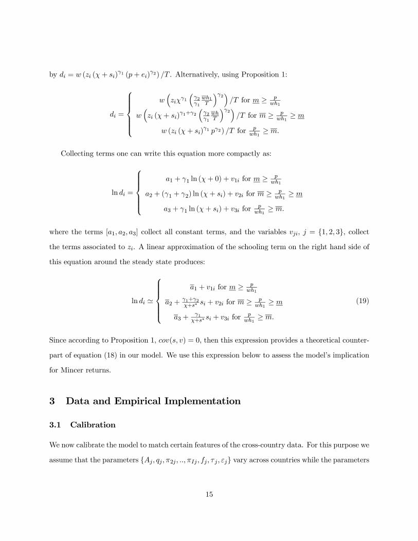
by di = w (zi (χ+ si)γ1 (p+ ei)

γ2) /T . Alternatively, using Proposition 1:

di =

⎧⎪⎪⎪⎪⎨⎪⎪⎪⎪⎩w³ziχ

γ1

³γ2γ1

wh1T

´γ2´/T for m ≥ p

wh1

w³zi (χ+ si)

γ1+γ2³γ2γ1

whT

´γ2´/T for m ≥ p

wh1≥ m

w (zi (χ+ si)γ1 pγ2) /T for p

wh1≥ m.

Collecting terms one can write this equation more compactly as:

ln di =

⎧⎪⎪⎪⎪⎨⎪⎪⎪⎪⎩a1 + γ1 ln (χ+ 0) + v1i for m ≥ p

wh1

a2 + (γ1 + γ2) ln (χ+ si) + v2i for m ≥ pwh1≥ m

a3 + γ1 ln (χ+ si) + v3i forpwh1≥ m.

where the terms [a1, a2, a3] collect all constant terms, and the variables vji, j = {1, 2, 3}, collect

the terms associated to zi. A linear approximation of the schooling term on the right hand side of

this equation around the steady state produces:

ln di '

⎧⎪⎪⎪⎪⎨⎪⎪⎪⎪⎩a1 + v1i for m ≥ p

wh1

a2 +γ1+γ2χ+s∗ si + v2i for m ≥

pwh1≥ m

a3 +γ1

χ+s∗ si + v3i forpwh1≥ m.

(19)

Since according to Proposition 1, cov(s, v) = 0, then this expression provides a theoretical counter-

part of equation (18) in our model. We use this expression below to assess the model’s implication

for Mincer returns.

3 Data and Empirical Implementation

3.1 Calibration

We now calibrate the model to match certain features of the cross-country data. For this purpose we

assume that the parameters {Aj , qj ,π2j , ..,πIj , fj , τ j , εj} vary across countries while the parameters

15

[α, δ, θ1,..,θI , T, γ,χ, z, ρ] are identical across countries. Individuals in the model are born at age

6 which roughly corresponds to the beginning of the schooling age in the data. Consistently, we

set χ = 6. Moreover, we consider 5 generations (I = 5), and a time period length T = 20. In

this specification, formal schooling takes place between the ages of 6 to 26, and individuals live

up a maximum of 106 years. Parameter α is set to 1/3 as in Mankiw, Romer and Weil (MRW,

1992), HJ, KRC, Bils and Klenow (BK, 2000), and others. Parameter δ is set such that the annual

depreciation rate is 0.06, which is the value assumed by HJ to compute the capital stocks that we

use. This requires to set δ = 1− (1− 0.06)20.

Calibration of πj and fj We estimate πij as follows. We take the US life table of total

population from National Vital Statistics Report by the US Census Bureau and, for each country

j, we adjust the US age-specific mortality rates to reproduce the life expectancy of country j as

reported by the World Bank. Mortality rates for ages 0 to 5 are adjusted using the World Bank

data on mortality rates under age 5. Mortality rates over ages 5 are multiplied by a factor which

allows to exactly replicate country’s j life expectancy. {πij}Ii=2 is computed, using the results of

the table, as the number of survivors at ages 36, 56, 76, and 96 respectively divided by the number

of survivors at age 6.

Fertility rates, fj , are computed using equation (2). According to this equation, the share of

population under 26 is given by n1 = (fπ2)−1 /

³PIj=1 πj · (fπ2)

−j´. We use data from the World

Population Prospects (2004) to compute n1 for each country.4

An important consideration is the year of the data used for these computations. Since the late

70’s mortality rates have increased significantly, particularly in Sub-Saharan Africa, due to the

HIV/AIDS pandemic. For this reason we choose 1980 demographic variables, which are still not

affected by the pandemic and are likely more relevant to explain economic performance up to the

mid 90’s when the pandemic became more pronounced. We also conduct experiments below to

assess the long run consequences of the HIV/AIDS pandemic.

Figure 4 shows the demographic data and the calibrated values of fertility and survival proba-4Given data restriction, our data on n1 actually corresponds to population under 24.

16

bilities. A salient feature of the data is that survival rates are very different across countries and

particularly low for very poor countries. The Figure also shows the estimated fertility rates relative

to the US. They also decrease significantly with income levels, exhibit substantial difference across

countries, and are particularly large for very poor countries.

Calibration of τ and εj In the model, G = τY . Accordingly, we set τ equal to the share of

government expenditures in GDP in 1995 from the Penn World Tables. Furthermore, we compute

εj for each country as εj = spHj/τ j , where s

pHj is the share of public expenditures in education to

GDP for 1995 according to UNESCO. Figure 5 shows the resulting tax rate, τ j , and Figure 2 shows

subsidy per pupil as a fraction of per capita GDP p/y = spHj/n1. While taxes decrease slightly

with income, subsidies clearly increase with income specially because the fraction of schooling age

children is systematically larger in poor countries than in rich countries.

Calibration of θ We calibrate θ = [θ1, ..θ5] to reproduce the life-cycle pattern of earnings.

For this purpose, we employ the estimates of BK. Using cross-country evidence on earnings, they

estimate that earnings at age i satisfy:

w(i) = a(s) · em(ex),

where ex stands for years of experience andm(ex) = 0.0512·ex−0.0071·(ex)2. Assuming 0 years of

experience for children, 20 for young adults, 40 for adults, and 60 for older adults, and no earnings

for elders, we estimate θ as θ = [θ1 = em(0)−m(20), θ2 = 1, θ3 = em(40)−m(20), θ4 = em(60)−m(20), θ5 =

0] which produces θ = [0.48, 1, 1.19, 0.80, 0].

Calibration of γ1, γ2 and ρ To calibrate the key parameters —γ1, γ2, and ρ— we target mo-

ments of the cross-country distributions of returns to schooling and the average years of schooling.

Returns to schooling are obtained from Psacharopoulos and Patrinos (2002), while average years

of schooling in each country are obtained from Barro and Lee for the year 1995. Following the

derivations in Section 3, we compute returns to schooling as rs = (γ1 + γ2) / (χ+ s) for a mixed

17

educational system, rs = γ1/ (χ+ s) for a pure public system, rs = (γ1 + γ2) /χ for a pre-school

only system, and rs = γ1/χ for a no-schooling regime. The equilibrium educational system —

whether mixed, public, or other— is obtained using the model (more precisely, Proposition 2) for

different potential values of γ1, γ2, and ρ. In these calculations, the values of other parameters are

set at their calibrated values already described. Importantly, the calibration of γ1, γ2, and ρ is in-

dependent of the parameter values described below (Aj and qj) and therefore robust to alternative

specification of those parameters.

Table 1: Calibration of γ1, γ2 and ρ

Data (1) (2) (3) (4) (5) (6) (7) (8)

γ2 - 0.100 0.200 0.250 0.300 0.350 0.400 0.450 0.500

γ1 - 1.080 1.035 0.969 0.893 0.803 0.722 0.637 0.579

ρ - 0.970 0.972 0.975 0.978 0.984 0.990 0.999 1.008

s 5.840 5.844 5.832 5.836 5.832 5.837 5.834 5.845 5.839

rs 0.097 0.097 0.097 0.097 0.097 0.097 0.098 0.097 0.097

sstd 2.890 0.986 1.042 1.124 1.239 1.403 1.554 1.658 1.633

rsstd 0.042 0.025 0.029 0.031 0.033 0.032 0.030 0.026 0.025

Table 1 reports statistics related to schooling and returns to schooling from the model and the

data for different possible choices of γ1, γ2 and ρ. In these experiments, γ2 is allowed to vary

(between 0 to 0.5) and γ1 and ρ are chosen to match the average years of schooling (s) and the

average returns to schooling (rs). The table illustrates different trade-offs in the choice of γ2. For

example, γ2 = 0.30 produces the best results in terms of the standard deviation of returns to

schooling (0.042 in the data vs 0.033 in the model), while γ2 = 0.45 produces the best results in

terms of matching the standard deviation of schooling (2.89 vs 1.658). In both cases, however,

the model falls short of explaining all variation in returns and schooling. We choose the following

parameters: γ2 = 0.40, γ1 = 0.722 and ρ = 0.99.

18

Calibration of qj Given parameters (α, δ, T, ρ, θ, τ j ,πij , fj) already obtained, and years of

schooling, sj , equations (16) and (17) can be used to solve for qjkj/yj and rj for each country.

On the other hand, HJ provide capital-output ratios for a group of countries for 1996. They

compute capital stocks using annual investments valued at common international prices rather

than at domestic prices. Therefore, their capital-output ratio corresponds to that of k/y instead of

qk/y, which allows domestic prices of capital, qj , to vary across countries. Given qjkj/yj predicted

from the model and kj/yj from the data, qj can be obtained.

3.2 Assessment

We now assess the ability of the model to fit evidence beyond the matching targets.

Schooling Panel A of Figure 6 compares schooling attainments in the data and in the model.

Although we only target the mean of schooling, the model is able to replicate the entire distribution

of schooling fairly well. The correlation between schooling in the data and in the model is 86%.

Years of schooling in the data range from a minimum of 0.69 to a maximum of 12.18, and in the

model they range between 1.73 and 8.55. Finally, the correlation between schooling and relative

incomes is 85.3% in the data, versus 82.8% in the model.

Returns to Schooling Panel B of Figure 6 and Table 2 compare returns to schooling in the

data and the model, as well as the predictions of two alternative models. The first model is that

of HJ who estimate returns to schooling as 13.4% for first four years of schooling, 10.1% for the

next four years, and 6.8% for the remaining years. The second model is one of the versions in BK

—their intermediate version with moderate decreasing returns to schooling. In this version, returns

to schooling satisfy the expression rs = 0.18 · s−0.28.

Our model is able to reproduce the overall pattern of decreasing returns as income level increases,

and 71% of the dispersion of returns. Similarly to the other two models, our model overpredicts

the correlation between returns and relative incomes and underpredicts the dispersion of returns.

However, it is encouraging that our model is comparable to alternative models despite the fact that

19

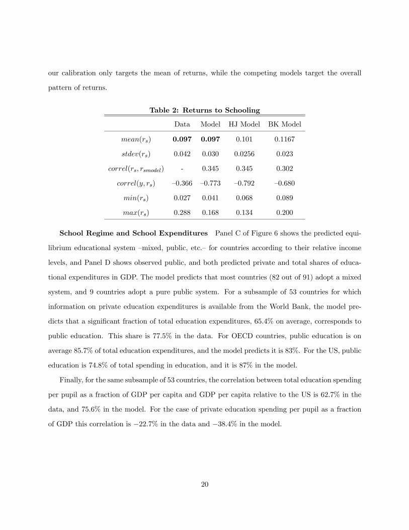
our calibration only targets the mean of returns, while the competing models target the overall

pattern of returns.

Table 2: Returns to Schooling

Data Model HJ Model BK Model

mean(rs) 0.097 0.097 0.101 0.1167

stdev(rs) 0.042 0.030 0.0256 0.023

correl(rs, rsmodel) - 0.345 0.345 0.302

correl(y, rs) —0.366 —0.773 —0.792 —0.680

min(rs) 0.027 0.041 0.068 0.089

max(rs) 0.288 0.168 0.134 0.200

School Regime and School Expenditures Panel C of Figure 6 shows the predicted equi-

librium educational system —mixed, public, etc.— for countries according to their relative income

levels, and Panel D shows observed public, and both predicted private and total shares of educa-

tional expenditures in GDP. The model predicts that most countries (82 out of 91) adopt a mixed

system, and 9 countries adopt a pure public system. For a subsample of 53 countries for which

information on private education expenditures is available from the World Bank, the model pre-

dicts that a significant fraction of total education expenditures, 65.4% on average, corresponds to

public education. This share is 77.5% in the data. For OECD countries, public education is on

average 85.7% of total education expenditures, and the model predicts it is 83%. For the US, public

education is 74.8% of total spending in education, and it is 87% in the model.

Finally, for the same subsample of 53 countries, the correlation between total education spending

per pupil as a fraction of GDP per capita and GDP per capita relative to the US is 62.7% in the

data, and 75.6% in the model. For the case of private education spending per pupil as a fraction

of GDP this correlation is −22.7% in the data and −38.4% in the model.

20

4 Human Capital Stocks

4.1 A Cross-Section

In this section we use the model to estimate human capital stocks for a set of 91 countries and

compare the results to some existing alternatives. According to equations (11) and (12), human

capital stocks are given by:

hj =

Ã(1− sj/T )n1jθ1 +

X2

θijnij

!z (χ+ sj)

γ ¡pj + e∗j¢1−γ .We use this formula to compute human capital stocks relative to the US, which eliminates the

need to estimate z, a parameter assumed to be identical across countries. Notice that once the

technological parameters are obtained, this formula could map observables nij , sj and pj + ej into

human capitals. However, due to the lack of reliable data on private education expenditures we

utilize the model’s predictions on total expenditures to compute human capital stocks. We also

report the results when only available information on public expenditures is employed.

Figure 7 and Table 3 characterize six different estimates of human capital stocks:

(1) those from our model, denoted CR;

(2) our model but using only public expenditures of education (CR-P);

(3) Hendricks’ (2002) estimates based on immigrants’ earnings in the US and no self-selection;5

(4) a version of BK that uses the formula h = ef(s)+0.0512·(age−s−6)−0.00071·(age−s−6)2, where f(s) =

(0.18/0.72) s0.72. These estimates are similar to those obtained by HJ;

(5) MRW’s estimates based on schooling (here we use primary plus secondary schooling as argued

by KRC);

(6) Cordoba and Ripoll’s (CR, 2004) estimates based on rural-urban wage gaps.

Panel A of Figure 7 and the first two columns of Table 3 characterize the human capital estimates5Using Hendricks’ notation, we compute human capital in country c as wη

c /wkc using the information in his Table

1. This measure of human capital includes both measured and unmeasured skills. See discussion in Section III.A inHendricks (2002).

21

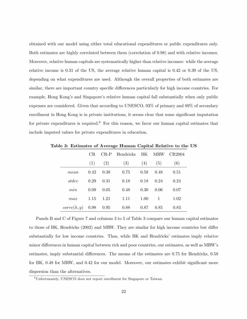
obtained with our model using either total educational expenditures or public expenditures only.

Both estimates are highly correlated between them (correlation of 0.98) and with relative incomes.

Moreover, relative human capitals are systematically higher than relative incomes: while the average

relative income is 0.31 of the US, the average relative human capital is 0.42 or 0.39 of the US,

depending on what expenditures are used. Although the overall properties of both estimates are

similar, there are important country specific differences particularly for high income countries. For

example, Hong Kong’s and Singapore’s relative human capital fall substantially when only public

expenses are considered. Given that according to UNESCO, 93% of primary and 89% of secondary

enrollment in Hong Kong is in private institutions, it seems clear that some significant imputation

for private expenditures is required.6 For this reason, we favor our human capital estimates that

include imputed values for private expenditures in education.

Table 3: Estimates of Average Human Capital Relative to the US

CR CR-P Hendricks BK MRW CR2004

(1) (2) (3) (4) (5) (6)

mean 0.42 0.38 0.75 0.58 0.48 0.51

stdev 0.29 0.31 0.18 0.18 0.24 0.24

min 0.09 0.05 0.48 0.30 0.06 0.07

max 1.15 1.21 1.11 1.00 1 1.02

corre(h, y) 0.98 0.95 0.88 0.87 0.85 0.83

Panels B and C of Figure 7 and columns 3 to 5 of Table 3 compare our human capital estimates

to those of BK, Hendricks (2002) and MRW. They are similar for high income countries but differ

substantially for low income countries. Thus, while BK and Hendricks’ estimates imply relative

minor differences in human capital between rich and poor countries, our estimates, as well as MRW’s

estimates, imply substantial differences. The means of the estimates are 0.75 for Hendricks, 0.58

for BK, 0.48 for MRW, and 0.42 for our model. Moreover, our estimates exhibit significant more

dispersion than the alternatives.6Unfortunately, UNESCO does not report enrollment for Singapore or Taiwan.

22

A further comparison is to the estimates of Cordoba and Ripoll (2004). They construct human

capital stocks for a set of countries weighting rural and urban estimates. They estimate urban

stocks using a standard Mincer approach (as in HJ) while rural stocks are Mincer type estimates

adjusted to account for the observed rural-urban wage gap in each country. Panel D of Figure 7 and

the last column of Table 3 compares our estimates to those of CR (2004). The 2004 estimates are

midway between our current estimates and those of BK, but both estimates provide a substantial

revision of human capital stocks relative to previous estimates, and they are at some extent similar

to those obtained by just taking average years of schooling relative to the US.

Finally, we can compare our human capital stocks with those of MS. Since they report average

human capital relative to the US by income deciles, we construct equivalent measures for our

estimates in Table 4. As shown in the table, our human capital estimates are consistently below

MS’s, proportionally more so for those countries below the 50th percentile. For instance, the average

country in the 50th− 60th percentile has 60% of US’s human capital according to MS, while it has

only 31% of US’s human capital according to our estimates. The only exception are those countries

in the lowest decile: they have 10% of US’s human capital according to our estimates, and 8%

according to MS’s.

Table 4 also reports BK’s human capital relative to the US. We use BK’s estimates to compute

the implied “quality” differentials in human capital across deciles for both our model and MS’s (see

last two columns). In particular, the ratio between our human capital and BK’s can be interpreted

as the relative human capital quality. As shown in Table 4, quality differences exists at all income

deciles in our estimates, while in MS they are only relevant for countries below the 40th percentile.

Specifically, while the average country in the 40th − 50th percentile range has about the same

human capital quality of the US according to MS, it has around 1/2 of the quality according to

our estimates. As noted above, the exception is in the lowest decile. Our human capital estimates

imply that a country in the lowest decile of the income distribution has a human capital quality

around 1/3 of the US, while it is around 1/4 according to MS. In conclusion, our human capital

estimates imply quantitatively important adjustments, proportionally more so for countries below

23

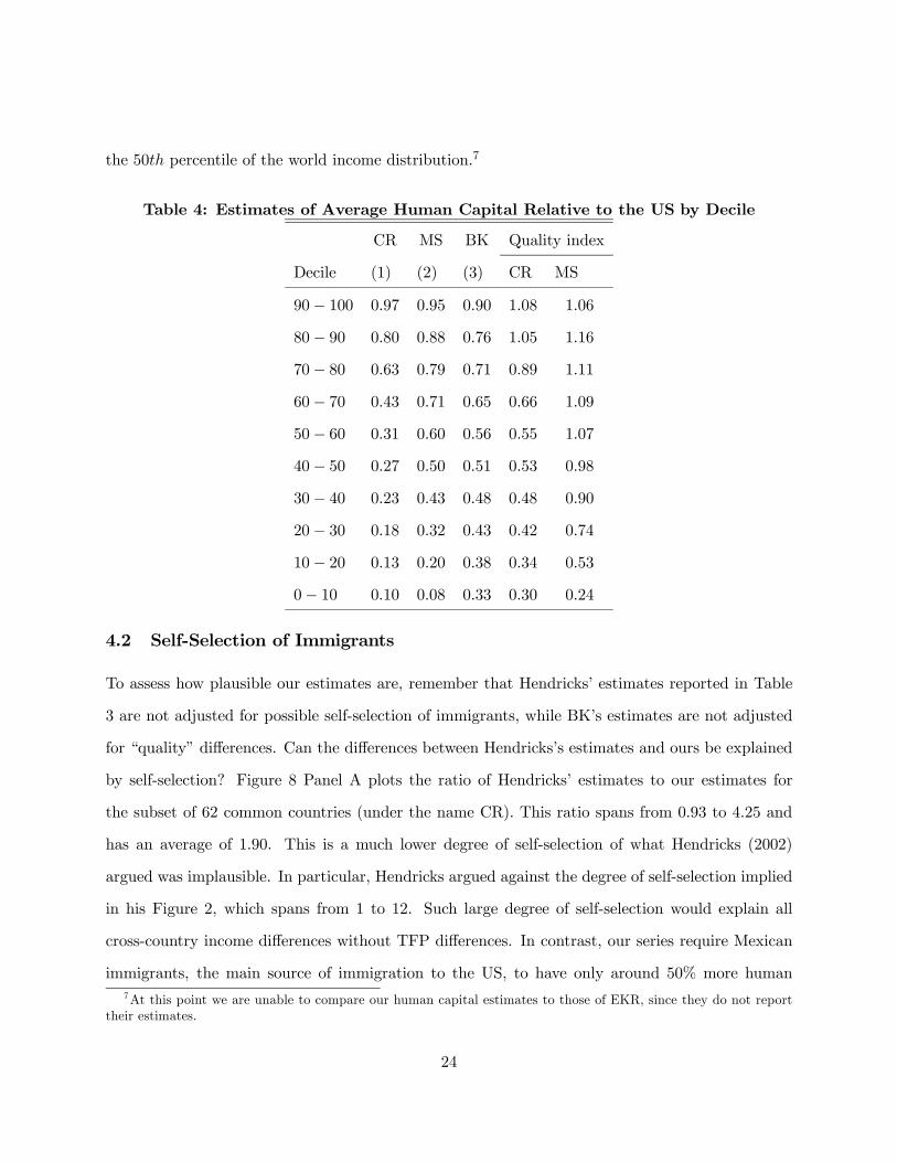
the 50th percentile of the world income distribution.7

Table 4: Estimates of Average Human Capital Relative to the US by Decile

CR MS BK Quality index

Decile (1) (2) (3) CR MS

90− 100 0.97 0.95 0.90 1.08 1.06

80− 90 0.80 0.88 0.76 1.05 1.16

70− 80 0.63 0.79 0.71 0.89 1.11

60− 70 0.43 0.71 0.65 0.66 1.09

50− 60 0.31 0.60 0.56 0.55 1.07

40− 50 0.27 0.50 0.51 0.53 0.98

30− 40 0.23 0.43 0.48 0.48 0.90

20− 30 0.18 0.32 0.43 0.42 0.74

10− 20 0.13 0.20 0.38 0.34 0.53

0− 10 0.10 0.08 0.33 0.30 0.24

4.2 Self-Selection of Immigrants

To assess how plausible our estimates are, remember that Hendricks’ estimates reported in Table

3 are not adjusted for possible self-selection of immigrants, while BK’s estimates are not adjusted

for “quality” differences. Can the differences between Hendricks’s estimates and ours be explained

by self-selection? Figure 8 Panel A plots the ratio of Hendricks’ estimates to our estimates for

the subset of 62 common countries (under the name CR). This ratio spans from 0.93 to 4.25 and

has an average of 1.90. This is a much lower degree of self-selection of what Hendricks (2002)

argued was implausible. In particular, Hendricks argued against the degree of self-selection implied

in his Figure 2, which spans from 1 to 12. Such large degree of self-selection would explain all

cross-country income differences without TFP differences. In contrast, our series require Mexican

immigrants, the main source of immigration to the US, to have only around 50% more human7At this point we are unable to compare our human capital estimates to those of EKR, since they do not report

their estimates.

24

capital than non-immigrants which is just a small fraction of the income gap between the two

countries (of 4.36 times).

Our series imply that on average immigrants have 90%more human capital than non-immigrants,

while the income gap on average is 10.27 times. Moreover, our 2004 estimates imply even much

lower degrees of self-selection than our current estimates, as shown in Figure 8 Panel B (33% on

average and 19% for Mexican immigrants).

Table 5: Selection of Immigrants

Upper Bound (1) (2) (3) (4) (5) (6) (7) (8)

γ2 - 0.10 0.20 0.25 0.30 0.35 0.40 0.45 0.50

γ1 - 1.08 1.03 0.96 0.89 0.80 0.72 0.63 0.57

ρ - 0.97 0.97 0.97 0.97 0.98 0.99 0.99 1.00

ss 3.070* 1.39 1.68 1.78 1.84 1.84 1.89 2.02 2.17

ssmax 13.06* 2.27 3.24 3.57 3.81 3.94 4.24 4.74 5.35

ssmin 0.690* 0.46 0.46 0.46 0.46 0.46 0.46 0.46 0.46

ssmex 2.060 1.21 1.46 1.55 1.54 1.48 1.48 1.54 1.62

pss 0.810* 0.64 0.70 0.71 0.72 0.71 0.72 0.73 0.75

pssmax 0.999* 0.89 0.96 0.97 0.97 0.97 0.98 0.99 0.99

pssmin 0.320* 0.49 0.47 0.45 0.44 0.42 0.44 0.47 0.47

pssmex 0.760* 0.57 0.64 0.66 0.66 0.64 0.64 0.66 0.67

ss = self-selection (Hendricks human capital/our human capital), ss = average self-selection,

pss = percentile position of immigrant, pss = average percentile.

Following Hendricks (2002, pg 208-9), we can also estimate the position of immigrants in the

earnings distribution of the source country implied by our model by assuming that earnings are

lognormal distributed, and using the Klaus Deininger and Lyn Squire’s (1996) Gini coefficients

for income.8 Figure 8B describes these results. The series denoted Hendricks is the upper bound

8The Gini coefficient of a log-normal distribution satisfies G = 2Φ³

σ√2

´− 1 where Φ is the standard normal

distribution. Thus, σ =√2Φ−1

¡1+G2

¢.

25

he provided. Our series imply much lower degree of self-selection than the upper bound for most

countries. Table 5 reports additional exercises for the different parametrization described in Table

1. Thus, for example, our benchmark parametrization (γ2 = 0.4) implies that the typical Mexican

immigrant is drawn from the 65 percentile of the earnings distribution. This is consistent with the

findings of Chiquiar and Hanson (2005), who find intermediate positive self-selection of Mexican

immigrants. They find that the typical immigrant is drawn from the 72 percentile. Table 5 also

illustrates that γ2 = 0.35 or γ3 = 0.4 produce the best results in terms of intermediate self-selection,

which lends further (and strong) support to our benchmark calibration.

5 The Sources of Income Differences

Development Accounting and the TFP Elasticity of Income A key parameter in our model

is γ2. Our assessment of the previous section lends support to our estimate of γ2 as it gives rise

to plausible predictions in terms of schooling, returns to schooling, and human capital estimates.

This parameter controls, among other things, the extent up to which TFP differences explain cross

country income differences. As stated in Equation (14), the elasticity of output to TFP in our

model is given by 11−α

11−γ2

= (1.5)× (1.6) = 2.4. This is a significantly larger elasticity than what

is obtained in model with exogenous human capital (of only 1.5). This elasticity is remarkably

similar to the EKR estimate of 2.8 despite the substantially different modeling approaches. A

crucial difference is that our model explains schooling differences mostly in terms of demographic

differences, while EKR abstract from demographic differences and rely on TFP differences only.

On the other hand, our elasticity is much lower than the MS estimate of around 9. Their large

elasticity implies that almost no differences in TFP are required to explain income differences,

while important TFP differences are still required in our model. There are two differences in our

modelling approaches that help explain the different results. First, TFP differences affect the steady

state levels of both quality and quantity of schooling (e and s) in MS while it only affects quality

of schooling in our model. An implication is that our model possess a balanced growth path but

MS does not. Second, our calibration targets cross-country differences in schooling and returns

26

to schooling. They instead target the earning gains between ages 25 to 50 in the US. Thus, they

assume that the technology of learning on the job is the same as the technology of learning in

school. We instead formulate and calibrate two different technologies and tie the estimation of γ2

to schooling attainments and returns to schooling rather than to the life-cycle earning profile.

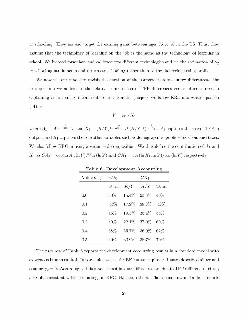
We now use our model to revisit the question of the sources of cross-country differences. The

first question we address is the relative contribution of TFP differences versus other sources in

explaining cross-country income differences. For this purpose we follow KRC and write equation

(14) as:

Y = A1 ·X1

where A1 ≡ A1

(1−α)(1−γ2) and X1 ≡ (K/Y )α

(1−α)(1−γ2) (H/Y γ2)1

(1−γ2) . A1 captures the role of TFP in

output, and X1 captures the role other variables such as demographics, public education, and taxes.

We also follow KRC in using a variance decomposition. We thus define the contribution of A1 and

X1 as CA1 = cov(lnA1, lnY )/V ar(lnY ) and CX1 = cov(lnX1, lnY )/var(lnY ) respectively.

Table 6: Development Accounting

Value of γ2 CA1 CX1

Total K/Y H/Y Total

0.0 60% 15.4% 23.8% 40%

0.1 52% 17.2% 29.8% 48%

0.2 45% 19.3% 35.4% 55%

0.3 40% 22.1% 37.0% 60%

0.4 38% 25.7% 36.0% 62%

0.5 30% 30.9% 38.7% 70%

The first row of Table 6 reports the development accounting results in a standard model with

exogenous human capital. In particular we use the BK human capital estimates described above and

assume γ2 = 0. According to this model, most income differences are due to TFP differences (60%),

a result consistent with the findings of KRC, HJ, and others. The second row of Table 6 reports

27

the results obtained in our model. Perhaps surprisingly, the role of TFP decreases significantly,

from 60% to 34%, when human capital is endogenous. It may seem surprising that the TFP

elasticity of income increases but its total contribution decreases. However, as Proposition 3 states,

not only the TFP elasticity increases but also the elasticity of the capital-output ratio increases.

The overall effect is an increase in the role of other factors and a reduction in the role of TFP in

explaining income differences. These results contrast to those of MS who find that, once variation

in demographics and the price of capital are taking into account, no differences in TFP are needed

to explain income differences. We find that TFP differences are still substantial, although not the

main source of income differences.

Counterfactuals We now use the full model to assess the sources of cross-country income differ-

ences. According to our model, countries differ in their incomes due to differences in fundamentals

Fj = [Aj ,πj , fj , τ , εj , qj ]. Denote Fji the i element of this vector. A way to assess the contribution

of a fundamental in explaining income differences is to equate the fundamental to its US value and

compute the resulting reduction in income dispersion. More precisely, define:

Φi = 1−var(ln yc(Fji = Fus,i))

var(ln y),

where yc(Fji = Fus,i) is the vector of counterfactual levels of outputs obtained when the parameter

Fji is equated to its US value, Fus,i. Thus, for example ΦA = 1 would mean that by equating

all TFP’s income differences would be eliminated. The results are surprising. The single more

important fundamental is the survival rate followed by TFP. According to the model, equating

mortality rates across countries would reduce the variance of log incomes in 51%, while equating

TFP would reduce that variance in 48%. The role of public education is also important. Equating

the share of education in the government expenditures would reduce income variance in 18%.

28

6 The Effects of the HIV/AIDS Pandemic in Development

As documented in the previous section, according to our model, mortality rates are a major deter-

minant of income differences. Although a general pattern of convergence in demographic variables

took place until recently, this pattern changed substantially with the HIV/AIDS pandemic. Panel

A in Figure 9 illustrates the changes in life expectancy between 1980 and 2003. Life expectancy fell

in many countries with already short life expectancy in 1980, while it increased in most countries

with already large life expectancy. The most dramatic cases are Botswana, Zimbabwe, Lesotho,

Zambia, and South Africa where life expectancy fell in 20, 16, 15, 13 and 11 years respectively

between 1980 to 2003.

A number of papers have tried to assess the short and long run effects of the AIDS pandemic

in development within a general equilibrium framework.9 Young (2005) provides an assessment

for South Africa under the assumptions that the epidemic disappears completely within a 50 years

period, that savings rate rates remain unchanged, and that student time is the only input in the

production of human capital. He finds that per capita income will increase for generations following

the end of the pandemic. In contrast, Arndt and Lewis (2000) find significant negative effects even

in the short run, and using a very simple model of human capital accumulation. Ferreira and Pessoa

(2003) and Corrigan, Glomm and Mendez (2004) study the effects of a more permanent change in

mortality rates and find that the epidemic has significant negative effects. Their human capital

models assume that student time is the only input the production of human capital.

We now use our model to assess the long-run development consequences of the HIV/AIDS

pandemic. For this purpose, we follow the process described in Section 3 to compute survival

probabilities for ages 6 and above using 2003 statistics on life expectancy at birth and mortality

rates under age 5. We feed the model with the new survival probabilities and calculate the predicted

levels of output, capital, and human capital. Results are shown in Figure 9. The model predicts

a 28% increase in the variance of log incomes mostly explained by substantial set backs in Africa.9Econometric exercises include Bloom and Mahal (1997), who find no major effect, and Ukpolo (2004) who finds

major effects.

29

Both physical and human capital fall substantially, although physical capital reacts more strongly.

Table 7: Long-run Effects of the AIDS Pandemic

Ferreira-Pessoa Cordoba-Ripoll

Ratio of Ratio of Change Fraction Old Adults

y s y s h k MLE Ms π4(1980) π4(2003)

Botswana 0.56 0.29 0.24 0.18 0.40 0.09 -20.08 -3.88 0.17 0.00

Zimbabwe 0.65 0.38 0.28 0.35 0.43 0.12 -16.62 -2.87 0.11 0.00

Zambia 0.67 0.49 0.35 0.57 0.49 0.17 -14.18 -2.41 0.06 0.00

Lesotho 0.74 0.54 0.26 0.04 0.41 0.10 -17.58 -4.08 0.09 0.00

South Africa 0.74 0.57 0.44 0.76 0.59 0.23 -12.41 -1.90 0.15 0.00

Kenya 0.79 0.62 0.51 0.61 0.65 0.05 -9.51 -1.37 0.11 0.01

Malawi 0.82 0.66 0.45 0.31 0.56 0.28 -9.45 -1.80 0.02 0.00

Algeria 1.16 1.34 1.29 1.20 1.17 1.57 +8.74 +0.77 0.25 0.51

Tunisia 1.18 1.38 1.27 1.20 1.16 1.54 +8.92 +0.73 0.31 0.58

Egypt 1.2 1.38 1.39 1.21 1.22 1.80 +9.63 +0.91 0.18 0.46

Table 7 reports our predictions and compares them to those of Ferreira and Pessoa (2003).10

Our predictions for schooling are somehow similar (and reasonable given the reductions in life

expectancy) but our predictions for output are very different, mainly due to dramatic falls in

capital stocks. The reason is that when individuals die younger, since they are at the upward

slopping part of their earning schedule, savings for retirement are dramatically reduced.11

10Results are not strictly comparable. Ferreira and Pessoa use 1985 demographics in their benchmark and 1999demographics in the experiment, while we use 1980 versus 2003 demographics.11As observed in Table 7, our results are the opposite to those of Young (2005). Part of the difference is that he

assumes that the pandemic will completely and linearly disappear within the next 50 years. We instead assume amore permanent effect. In addition, Young does not consider the effects on savings, but only on human capital andfertility.

30

7 Concluding Comments

Using a life-cycle model with public and private spending in schooling, we find that differences in

mortality rates are at least as important as TFP differences in accounting for the variance of log

incomes. In particular, elimination of TFP differences would reduce the variance of log income in

48%, while elimination of mortality differences would do so by 51%. In addition, the equilibrium

of our model implies a set of human capital estimates for all countries in the sample. We find that

these estimates suggest a larger dispersion than standard Mincer-equation estimates. In particular,

human capital in poorer countries is substantially lower.

In an apparent contradiction to our results, Acemoglu and Johnson (2006) find that increases in

life-expectancy since 1950 did not have much effect on output growth. However, we view our paper

and theirs as complementary. First, the reduction in mortality that they refer to is mostly children

mortality. In our model, this would be the same as an increase in fertility rates and therefore

should actually decrease output. The reason is that having more children around dilutes public

expenditures in education and can actually reduce human capital per worker rather than increase

it, depending on the response of years of schooling. Second, since different from Acemoglu and

Johnson we mostly consider adult mortality, our model is suitable for analyzing events such as the

HIV/AIDS pandemic, while theirs is not. Our results mainly suggest that understanding the origin

of differences in mortality rates is an important item in the research agenda in cross-country income

inequality.

31

Appendix

Demographics Note that by definition of πi one has that Ni,t = πiN1,t−(i−1). Thus,

Nt =IXi=1

Nit = N1t

IXi=1

NitN1t

= N1t

IXi=1

πiN1,t−(i−1)N1t

.

In addition, from (1), N1t = (fπ2)i−1N1,t−(i−1). Thus,

N1,tNt

=1PI

i=1πi

(fπ2)i−1

.

Finally,NitNt

=N1tNt

NitN1t

=N1tNt

πiN1,t−(i−1)N1t

=N1tNt

πi

(fπ2)i−1 .

These two equation can be written as in (2).

Solution to the Individual Problem Note that the set of budget constraints (5) can be writtenas:

c1 + e = wh1 (1− s/T ) ;IXi=2

ci(1 + r)i−2

=IXi=2

whi(1 + r)i−2

= Θwh2 (20)

where Θ (r) ≡PIi=2

θi(1+r)i−2 = 1+

PIi=3

θi(1+r)i−2 > 1. The individual problem can thus be written

as:

maxs,e,{ci}Ii>2

+ ln (wh1 (1− s/T )− e) +IXi>2

πiρi−1 ln (ci)

+ρπ2 ln

"Θwz(χ+ s)γ1 (p+ e)γ2 −

IXi>2

ci(1 + r)i−2

#+μs+ λe

where μ and λ are Lagrange multipliers. An optimal solution must satisfy:

s : wh1/T = ρπ2c1c2γ1Θwh2

1

χ+ s+ μ (21)

e : 1 = ρπ2c1c2γ2Θwh2

1

p+ e+ λ (22)

ci : ρπ21

c2

1

(1 + r)i−2= πiρ

i−1 1

cifor i = 3, .., I. (23)

32

The last equation produces:

ci =πiπ2[ρ (1 + r)]i−2 c2 for i = 3, .., I (24)

Using this result and (20) one obtains:

c2 = Θwh2 −IXi=3

ci(1 + r)i−2

= Θwh2 − c2IXi=3

πiπ2

ρi−2 (25)

=Θwh2

1 +PIi=3

πiπ2ρi−2

.

Then, one can use (24) and (25) to write cj more generally as:

cj = Θj (r)wh2 for j = 2, .., I.

where

Θj(r) ≡πjπ2[ρ (1 + r)]j−2Θ

1 +PIi=3

πiπ2ρi−2

=

PIi=2 θi (1 + r)

j−iPIi=2

πiπjρi−j

.

Furthermore, one can obtain ai as:

ai = whi + (1 + r)ai−1 − ci

so that

a1 = 0,

a2 = (1−Θ2)wh2,...

ai = (θi −Θi)wh2 + (1 + r) ai−1.for i = 3, .., I.

Alternatively

a3 = [(θ3 −Θ3) + (1 + r) (1−Θ2)]wh2a4 =

h(θ4 −Θ4) + (1 + r) (θ3 −Θ3) + (1 + r)2 (1−Θ2)

iwh2

ai = wh2

iXj=2

(1 + r)i−j (θj −Θj) for i = 2, ..., I.

Moreover,

qK =IXi=1

niai = wh2

IXi=2

ni

iXj=2

(1 + r)i−j (θj −Θj(r)) . (26)

33

Define Φ(r) ≡PIi=2 ni

Pij=2 (1 + r)

i−j (θj −Θj(r)). Then

qK = wh2Φ(r) (27)

Furthermore, using (9) and (11):

qK

Y=

(1− α) (1− τw)

(1− s/T )n1θ1 +P2 θini

Φ(r) (28)

Moreover, PIi=1NiaiPI

i=1πi+1πiNiai

=

PIi=2 niwh2

Pij=2 (1 + r)

i−j (θj −Θj)PIi=2

πi+1πiniwh2

Pij=2 (1 + r)

i−j (θj −Θj)

=

PIi=2 ni

Pij=2 (1 + r)

i−j (θj −Θj)PIi=2

πi+1πiniPij=2 (1 + r)

i−j (θj −Θj)

Interior Solution: s∗ ≥ 0 and e∗ ≥ 0 Consider first interior solutions (μ = 0 and λ = 0).From (21) and (22) one obtains:

e =γ2γ1

wh1T

(χ+ s)− p. (29)

Moreover, from (22), (25) and (4) it follows that:

p+ e = ρπ2γ2c1c2Θwh2

= ρπ2γ2wh1(1− s/T )− e

c2Θwh2

= ρπ2

Ã1 +

IXi=3

πiπ2

ρi−2!γ2 (wh1(1− s/T )− e)

= eργ2 (wh1(1− s/T )− e− p+ p) ,or

p+ e =eργ2ψwh11 + eργ2ψ

µ1− s/T + p

wh1

¶(30)

where eρ ≡ PIi=2 ρ

i−1πi. Equating this expression to (29) and solving for s produces the optimallevel of schooling in an interior solution:

s∗ =eργ1ψT

1 + eρ (γ2 + γ1)ψ

∙p

wh1−m

¸if

p

wh1≥ m. (31)

The last condition guarantees that s∗ ≥ 0. In addition, substituting this result into (29) producesthe optimal level of private expenditures for an interior solution:

e∗ =1 + eρψγ1

1 + eρ (γ1 + γ2)ψ

∙m− p

wh1

¸wh1 if m ≥

p

wh1. (32)

34

The last condition guarantees that e∗ ≥ 0. Furthermore, from (7) and (29):

h2 = z(χ+ s)γ1 (p+ e)γ2

= z(χ+ s)

µγ2γ1

wh1T

¶γ2

= z(χ+ s)

µ1− γ

γ

wθ1T

¶γ2

hγ2p

Corner Solution: e = 0 and s ≥ 0 Next, consider corner solutions of the form e = 0 ands ≥ 0. From equations (21), (25) and (4) one obtains:

χ+ s

T= ρπ2γ1Θ

c1c2

h2h1= ρπ2γ1Θ

wh1(1− s/T )Θwh2

1+PIi=3

πiπ2

ρi−2

h2h1= eργ1(1− s/T )

and solving for s gives:

s∗ =eργ1T − χ

1 + eργ1 . (33)

Furthermore, e = 0 is optimal if λ ≥ 0 or

p ≥ ρπ2γ2c1c2Θwh2 = ρπ2γ2

wh1(1− s∗/T )Θwh2

1+PIi=3

πiπ2

ρi−2

Θwh2

= eργ2wh1µ1− eργ1 − χ/T

1 + eργ1¶= eργ2wh1 1 + χ/T

1 + eργ1or equivalently p

wh1≥ m.

Corner Solution: s∗ = 0 and e∗ ≥ 0 Now consider a corner solution of the form s = 0 ande ≥ 0. In this case, equation (30) is still valid because it does not use (21). Imposing s = 0 intothis equation and solving for e produces:

e∗ =eργ2wh1 − p1 + eργ2 if

p

wh≤ eργ2.

One also needs to check that μ ≥ 0. From (21) and (25) this is the case if:

wh1/T ≥ ρπ2γ1c1c2Θwh2

1

χ= ρπ2γ1ψ

wh1 − e∗Θwh2

1+PIi=3

πiπ2

ρi−2

Θwh21

χ

= eργ1µwh1 − eργ2wh1 − p1 + eργ2¶1

χ

= eργ1µwh1 + p1 + eργ2¶1

χ

35

This inequality can be rewritten as m ≥ pwh . Thus, this case requires m ≥

pwh and ργ2ψ ≥ p

wh .However, one can check that the first inequality implies the second under Assumption 1.

Solution to the general equilibrium problem >From (9), (11) and (6) one has that:

wh1 = (1− τw) (1− α)y

hh1 =

(1− τw) (1− α) y/n1

1− s/T +P2

θiniθ1n1

(34)

Define bm ≡ m1+χ/T+m1+eρψ +

P2

θiniθ1n1

andω =

²τ

(1− τw) (1− α)

Mixed Education Equation (13) states that pwh1

= ω³1− s∗/T +

P2

θiniθ1n1

´. For the case

of mixed education we then have that:

p

wh1= ω

Ã1 +

X2

θiniθ1n1

− eργ11 + eρ (γ1 + γ2)

∙p

wh1−m

¸!

Solving for pwh produces:

p

wh1=

1 + eρ (γ1 + γ2)

1 + eρ (γ1ω + γ1 + γ2)ω

Ã1 +

X2

θiniθ1n1

+eργ1m

1 + eρ (γ1 + γ2)

!

m ≡ eργ2 (1 + χ/T )

1 + eργ1 ; m =(1 + eργ2)χ/Teργ1 − 1

Alternatively, one can use the definitions of m and m to rewrite this expression as:

p

wh1=

1 + eρ (γ1 + γ2)

1 + eρ (γ1ω + γ1 + γ2)ω

ÃX2

θiniθ1n1

+1 + χ/T + (1 + eργ1)m

1 + eρ (γ1 + γ2)

!

Substituting the first expression into (31) and the second expression into (32), using (34) andsimplifying produces:

s∗ =eργ1T hω ³1 +P2

θiniθ1n1

´−m

i1 + eρ (γ1ω + γ1 + γ2)

;

e∗ =wh1 (1 + eργ1)

1 + eρ (γ1ω + γ1 + γ2)

"m− ω

Ã1 + χ/T +m

1 + eρ +X2

θiniθ1n1

!#

36

or defining sH ≡ N1(p+e)Y = ετ +

13e

Y , which uses (10), one obtains

sH = ετ +(1− τw) (1− α)

1− s/T +P2

θiniθ1n1

(1 + eργ1) mbm [bm− ω]

1 + eρ (γ1ω + γ1 + γ2)

Corner Solution: e∗ = 0 and s∗ ≥ 0 The solution for s∗ is given by (33) and sH = ετ .

Corner Solution: s∗ = 0 and e∗ ≥ 0. For this case (13) produces

p

wh1= ω

Ã1 +

X2

θiniθ1n1

!

and from Proposition 1

e∗

wh1=eργ2 − ω

³1 +

P2

θiniθ1n1

´1 + eργ2 .

Moreover, using (34)N1e

∗

Y= wh

e∗

wh1

N1Y=(1− τw) (1− α)

1 +P2

θiniθ1n1

e∗

wh1

so that

sH = ετ +(1− τw) (1− α)

1 +P2

θiniθ1n1

eργ2ψ − ω³1 +

P2

θiniθ1n1

´1 + eργ2ψ .

Other General Equilibrium Results Per-capita output can be written as:

y = Akα (h)1−α = A

µk

y

¶αµ h

yγ2

¶1−αyα+γ2(1−α)

= A1

(1−α)(1−γ2)

µk

y

¶ α(1−α)(1−γ2)

µh

yγ2

¶ 11−γ2

Moreover, notice that in a stationary equilibrium h satisfies, using (11) and (12):

h =

Ã(1− s∗/T )n1θ1 +

X2

θini

!z (χ+ s∗)γ1 (p+ e)γ2

=

Ã(1− s∗/T )n1θ1 +

X2

θini

!z (χ+ s∗)γ1

µn1 (p+ e)

y

y

n1

¶γ2

=

Ã(1− s∗/T )n1θ1 +

X2

θini

!z (χ+ s∗)γ1 (s∗H/n1)

γ2 yγ2

37

so thath

yγ2=

Ã(1− s∗/T )n1θ1 +

X2

θini

!z (χ+ s∗)γ1 (s∗H/n1)

γ2 .

38

References

[1] Arndt, C. and Lewis, J.D. (2000), “The Macro implications of HIV/AIDS in South Africa: apreliminary assessment.” South African Journal of Economics 68, 856-887.

[2] Barro, R. and Jong-Wha Lee (2000), “International Data on Educational Attainment. Updatesand Implications.” NBER Working Paper # 7911.

[3] Bils, M. and Klenow, P. “Does Schooling Cause Growth?” American Economic Review, De-cember 2000, 90(5), pp. 1160-83.

[4] Bloom, D. E. and Mahal, A. S “Does AIDS Pendemic Threaten Economic Growth,” Journalof Econometrics 77: 105-24.

[5] Chiquiar, D. and Hanson, G. H. “International Migration, Self-Selection, and the Distributionof Wages: Evidence from Mexico and the United States” Journal of Political Economy, 2005,Vol 113, No. 3, pp. 239-281.

[6] Córdoba, J. C. and Ripoll, M. “Agriculture, Aggregation, Wage-Gaps, and Cross-CountryIncome Differences,” Mimeo, 2004.

[7] Corrigan, P., Glomm, G. and Mendez, F. “AIDS crisis and Growth,” Journal of DevelopmentEconomics 77 (2005) 107-124.

[8] Erosa, A.; Korseshkove, T. and Restuccia D. “On the Aggregate and Distributional Implica-tions of Productivity Differences across Countries.” Mimeo, University of Toronto, February2006.

[9] Ferreirra, P.C and Pessoa, S.A. “The Costs of Education, Longevity and the Poverty of Na-tions,” Mimeo 2003.

[10] Ferreirra, P.C and Pessoa, S.A. “The Long-Run Economic Impact of AIDS,” Mimeo 2003.

[11] Hall, Robert E. and Jones, Charles I. “Why Do Some Countries Produce So Much MoreOutput Per Worker Than Others?” Quarterly Journal of Economics, February 1999, 114(1),pp. 83-116.

[12] Hendricks, L. “How Important Is Human Capital for Development? Evidence from ImmigrantEarnings?” American Economic Review, March 2002, 92(1), pp. 198-219.

[13] Huggett, M., Ventura, G., and Yaron, A. “Human capital and earnings distribution dynamics,”Journal of Monetary Economics, 2006, Elsevier, vol. 53(2), pages 265-290, March

[14] Klenow, Peter J. and Rodríguez-Clare, Andrés. “The Neoclassical Revival in Growth Eco-nomics: Has It Gone Too Far?” in Ben S. Bernanke and Julio J. Rotemberg, eds., NBERMacroeconomics annual 1997. Cambridge, MA: MIT Press, 1997a, pp. 73-103.

[15] Mankiw, N. Gregory; Romer, David and Weil, David N. “A Contribution to the Empirics ofEconomic Growth.” Quarterly Journal of Economics, May 1992, 107 (2), pp. 407-37.

39

[16] Manuelli, R. E. and Seshadri A. “Human Capital and the Wealth of Nations.” Mimeo, Uni-versity of Wisconsin-Madison, June 2005.

[17] Psacharopoulos, G. and Patrinos H A. “Returns to Investment in Education: A Further Up-date.” Policy Research Working Paper 2881, The World Bank, September 2002.

[18] Ukpolo, V. “AIDS Epidemic and Economic Growth: Testing for Causality,” Journal of Asianand African Studies 39(3), 2004.

[19] Young, Alwyn. “In Sorrow to Bring Forth Children: Fertility amidst the Plague of HIV.”Mimeo 2005.

[20] Young, Alwyn. “The Gift of the Dying: The Tragedy of AIDS and the Welfare of FutureAfrican Generations.” Quarterly Journal of Economics, May 2005, 120 (2), pp. 420-66.

40

Figure 1% Enrollment in Public Schools

0

10

20

30

40

50

60

70

80

90

100

0.0 0.1 0.2 0.3 0.4 0.5 0.6 0.7 0.8 0.9 1.0

Per capita GDP relative to US

PrimarySecondary

Source: UNESCO

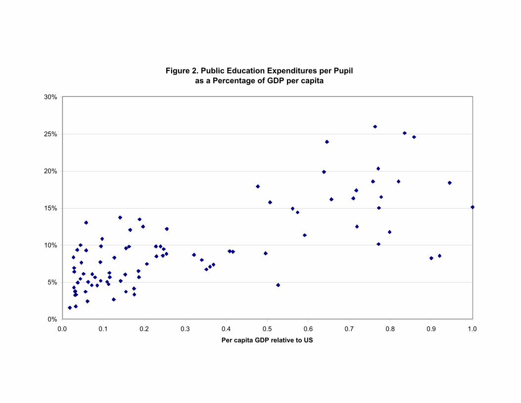
Figure 2. Public Education Expenditures per Pupil as a Percentage of GDP per capita

0%

5%

10%

15%

20%

25%

30%

0.0 0.1 0.2 0.3 0.4 0.5 0.6 0.7 0.8 0.9 1.0

Per capita GDP relative to US

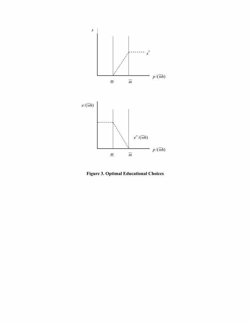
Figure 3. Optimal Educational Choices

)/( hwp m m

)/( hwe

)/(* hwe

s

)/( hwp m m

s*

Figure 4Demographics

Life Expectancy at Birth

30

40

50

60

70

80

0.0 0.1 0.2 0.3 0.4 0.5 0.6 0.7 0.8 0.9 1.0

Per capita GDP relative to US 1995

Yea

rs

Congo D.R

Population Under 24

0%

10%

20%

30%

40%

50%

60%

70%

80%

0.0 0.1 0.2 0.3 0.4 0.5 0.6 0.7 0.8 0.9 1.0

Per capita GDP relative to US 1995

Survival Probabilities1980

0.00

0.10

0.20

0.30

0.40

0.50

0.60

0.70

0.80

0.90

1.00

0.0 0.1 0.2 0.3 0.4 0.5 0.6 0.7 0.8 0.9 1.0

Per capita GDP relative to US 1995

Yea

rs

phi2 Phi3 Phi4 Phi5

Fertility Rates1980

0.0

0.5

1.0

1.5

2.0

2.5

3.0

3.5

0.0 0.1 0.2 0.3 0.4 0.5 0.6 0.7 0.8 0.9 1.0

Per capita GDP relative to US 1995

Yea

rs

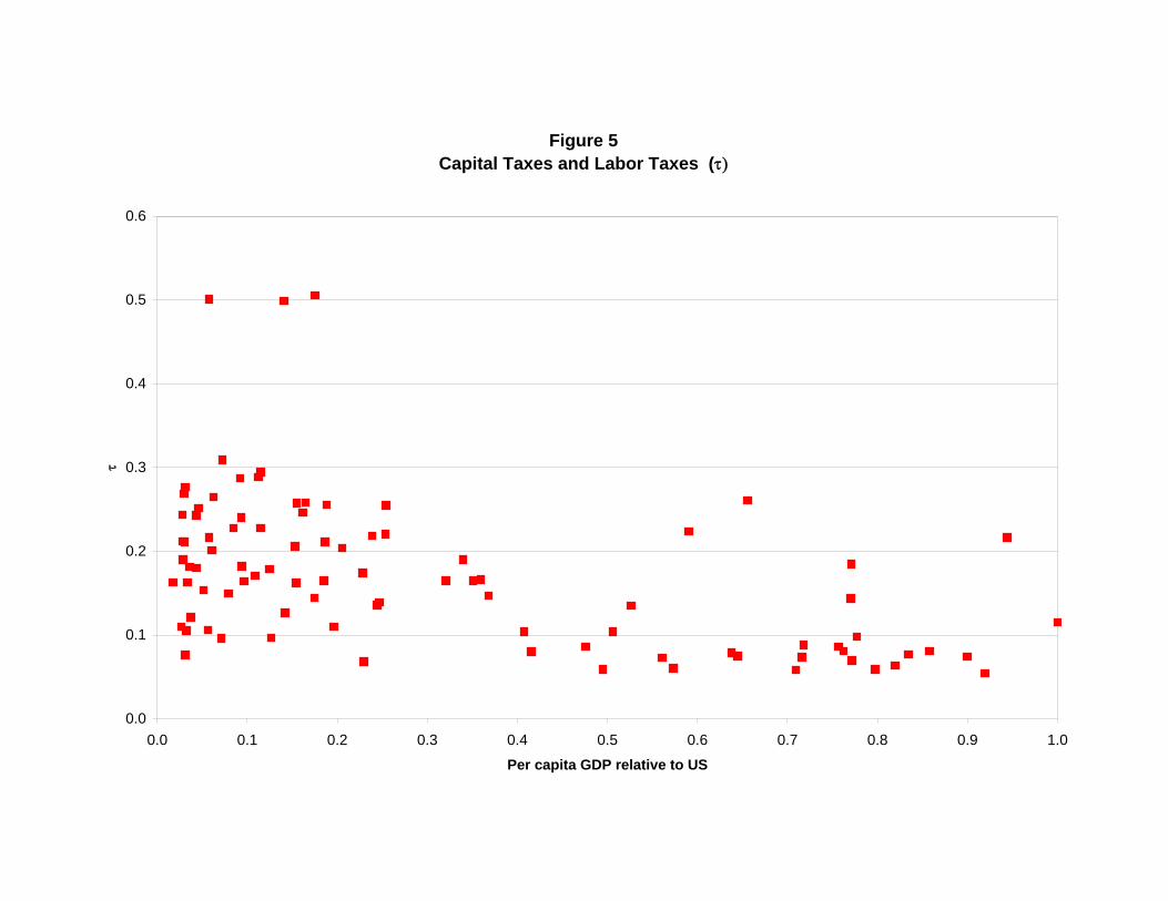
Figure 5Capital Taxes and Labor Taxes (τ)

0.0

0.1

0.2

0.3

0.4

0.5

0.6

0.0 0.1 0.2 0.3 0.4 0.5 0.6 0.7 0.8 0.9 1.0

Per capita GDP relative to US

τ

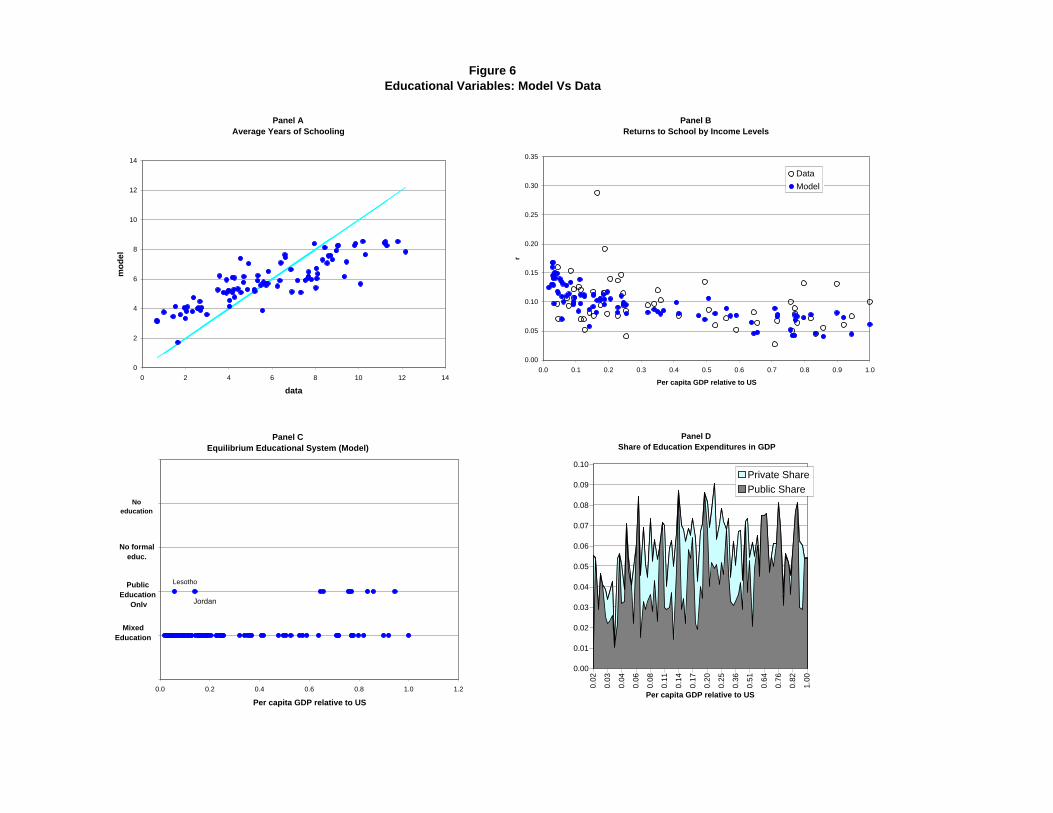
Figure 6Educational Variables: Model Vs Data

Panel CEquilibrium Educational System (Model)

0.0 0.2 0.4 0.6 0.8 1.0 1.2

Per capita GDP relative to US

MixedEducation

PublicEducation

Only

No formal educ.

No education

Lesotho

Jordan

Panel AAverage Years of Schooling

0

2

4

6

8

10

12

14

0 2 4 6 8 10 12 14

data

mod

elPanel B

Returns to School by Income Levels

0.00

0.05

0.10

0.15

0.20

0.25

0.30

0.35

0.0 0.1 0.2 0.3 0.4 0.5 0.6 0.7 0.8 0.9 1.0

Per capita GDP relative to US

r

DataModel

0.02

0.03

0.04

0.06

0.08

0.11

0.14

0.17

0.20

0.25

0.36

0.51

0.64

0.76

0.82

1.00

0.00

0.01

0.02

0.03

0.04

0.05

0.06

0.07

0.08

0.09

0.10

Per capita GDP relative to US

Panel DShare of Education Expenditures in GDP

Private SharePublic Share

Figure 7Human Capital Stocks Estimates

Panel AHuman Capital Estimates with Total and Only Public Expenditures

(Relative to US)

0.00

0.10

0.20

0.30

0.40

0.50

0.60

0.70

0.80

0.90

1.00

0.00 0.10 0.20 0.30 0.40 0.50 0.60 0.70 0.80 0.90 1.00

Per capita GDP relative to US

hu

man

cap

ital r

elat

ive

to U

S

(CR) - Model with TotalEducation ExpendituresModel with Only PublicEducation Expenditures45º

Singapure

Hong-Kong

Taiwan

Panel BHuman Capital Stocks Compared to Other Estimations

(Relative to the US)

0.00

0.10

0.20

0.30

0.40

0.50

0.60

0.70

0.80

0.90

1.00

0.00 0.10 0.20 0.30 0.40 0.50 0.60 0.70 0.80 0.90 1.00

Per capita GDP relative to US

hu

man

cap

ital r

elat

ive

to U

S

Cordoba & Ripoll (2006)Bils & Klenow (2001)Hendricks (2002)45º

Panel DHuman Capital Stocks Compared to Own Previous Estimates

(Relative to US)

0.00

0.10

0.20

0.30

0.40

0.50

0.60

0.70

0.80

0.90

1.00

0.00 0.10 0.20 0.30 0.40 0.50 0.60 0.70 0.80 0.90 1.00Per capita GDP relative to US

hu

man

cap

ital

rel

ativ

e to

US

Cordoba & Ripoll (2006)Cordoba & Ripoll (2004)45º

Panel CHuman Capital Stocks Compared to Other Estimations

(Relative to the US)

0.00

0.10

0.20

0.30

0.40

0.50

0.60

0.70

0.80

0.90

1.00

0.00 0.10 0.20 0.30 0.40 0.50 0.60 0.70 0.80 0.90 1.00Per capita GDP relative to US

hu

man

cap

ital

rel

ativ

e to

US

Mankiw, Romer & Weil(1991, primary+secondary)Cordoba & Ripoll(2006)

45º

Figure 8Self-Selection of Immigrants

(A)Implied Self-Selection of Immigrants

(Human Capital Immigrant relative to non-immigrant)

0.5

1.0

1.5

2.0

2.5

3.0

3.5

4.0

4.5

5.0

0.0 0.1 0.2 0.3 0.4 0.5 0.6 0.7 0.8 0.9 1.0

Per capita GDP relative to US

τ

CR (2004)

CR

(B)Predicted Position of Immigrants in Source Country Earnings Distribution

35%

45%

55%

65%

75%

85%

95%

0.0 0.1 0.2 0.3 0.4 0.5 0.6 0.7 0.8 0.9 1.0

Per capita GDP relative to US

hu

man

cap

ital

rel

ativ

e to

US

CR 2004

CR

Hendricks

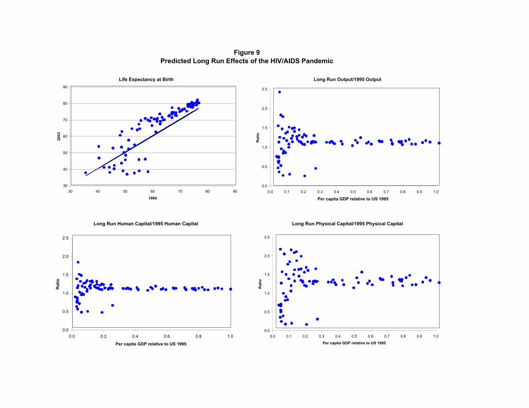
Figure 9Predicted Long Run Effects of the HIV/AIDS Pandemic

Life Expectancy at Birth

30

40

50

60

70

80

90

30 40 50 60 70 80 90

1980

2003

Long Run Output/1995 Output

0.0

0.5

1.0

1.5

2.0

2.5

0.0 0.1 0.2 0.3 0.4 0.5 0.6 0.7 0.8 0.9 1.0

Per capita GDP relative to US 1995

Rat

io

Long Run Human Capital/1995 Human Capital

0.0

0.5

1.0

1.5

2.0

2.5

0.0 0.2 0.4 0.6 0.8 1.0

Per capita GDP relative to US 1995

Rat

io

Long Run Physical Capital/1995 Physical Capital

0.0

0.5

1.0

1.5

2.0

2.5

0.0 0.1 0.2 0.3 0.4 0.5 0.6 0.7 0.8 0.9 1.0

Per capita GDP relative to US 1995

Rat

io