AIAA JOURNALVol. 37, No. 2, February 1999

Thermoviscoelastic Analysis of Composite Structures Usinga Triangular Flat Shell Element

Daniel C. Hammerand¤ and Rakesh K. Kapania†

Virginia Polytechnic Institute and State University, Blacksburg, Virginia 24061-0203

To accurately model the structural response of � ber-reinforced polymer-matrix composites, it is necessary toaccount for viscoelastic behavior of the polymer matrix. Therefore, the geometrically linear dynamic analysiscapability of a recently developed triangular � at shell element for elastic composite structures is extended hereto include thermoviscoelasticity. The � at shell element is the combination of the discrete Kirchhoff theory platebending element and a membrane element similar to the Allman triangle, but derived by transforming the linearstrain triangle element. Linear viscoelastic composite materials are modeled, resulting in the relaxation modulibeing expressed as Prony series. Hygrothermorheologically simple materials are considered for which a change inthe hygrothermal environment results in a horizontal shifting of the relaxation moduli curves on a log timescale, inaddition to the usual hygrothermal loads. The resulting hereditary integral terms are evaluated using a recursionrelationship requiring only the previous two solutions. The Newmark method is used to incorporate the inertiaterms. Numerical examples are presented to demonstrate the accuracy of the present formulation when comparedwith correspondence principle solutions and results available in the literature.

Introduction

E XAMPLES of viscoelastic materials include metals at hightemperatures, concrete, and polymers. For � ber-reinforced

polymer-matrix composites, the polymer matrix is typically vis-coelastic, whereas the � bers are elastic. For polymers, the elasticpart of the material response results from the polymer chains beingstretched by the applied stress. The viscous response of polymersresults from several relaxationmechanisms, such as motion of side-chain groups, reorientationof chain segments relative to each other,and the translationof entiremoleculespastone another in the case oflinear amorphous polymers in the rubbery-�ow region.1 Increasingthe temperature and moisture results in the viscous response beingaccelerated, as has been observed experimentally.2

For most amorphous polymers, experiments indicate that chang-ing the temperatureand moisture results in a simple horizontalshift-ing of the relaxationmodulus on a log timescale. Such materials arereferredto as beinghygrothermorheologically simple. For thesema-terials, the relaxationmodulus (viscoelasticstress response to a unitapplied strain) at the real temperature T , moisture H , and time t canbe related to the relaxation modulus at the reference temperatureTref, reference moisture Href, and reduced time ³ by

E.T; H; t/ D E.Tref; Href; ³/ .1/

where the reducedtime and the real time are relatedby the horizontalshift factor AT H as follows:

³ Dt

0

dt 0

AT H [T .t 0/; H .t 0/].2/

Although often found to be accurate, a simple horizontalshiftingis not valid for multiphase or semicrystalline polymers in general.For two-phasepolymers,horizontalshiftingalone still will be accu-rate if there is one dominant phase. In addition to using horizontalshifting, vertical shifting can be included in accounting for the ef-fects of physical aging or semicrystallization.Besides hastening itsviscous response, increasing a polymer’s temperature leads to an

Received March 16, 1998; presented as Paper 98-1763 at the AIAA/ASME/ASCE/AHS/ASC 39th Structures, Structural Dynamics, and Mate-rials Conference, Long Beach, CA, April 20–23, 1998; revision receivedOct. 1, 1998; accepted for publication Oct. 6, 1998. Copyright c° 1998 byDaniel C. Hammerand and Rakesh K. Kapania. Published by the AmericanInstitute of Aeronautics and Astronautics, Inc., with permission.

¤Graduate Research Assistant, Department of Aerospace and Ocean En-gineering. Student Member AIAA.

†Professor, Department of Aerospace and Ocean Engineering. AssociateFellow AIAA.

increase in the elastic stiffness of a rubbery network and a decreasein the density ½ that will decrease the relaxation modulus, becausethe relaxationmodulus obviously depends on the amount of matterper unit cross-sectional area.1 This results in an additional verticalshifting, with the vertical shift factor ½T=½refTref multiplying theright-hand side of Eq. (1).1

Related WorksLinear viscoelastic stress analysis can be performed in the time,

complex frequency, or Laplace domains. For general load histories(including hygrothermal loads) and viscoelastic material proper-ties, direct time integration schemes appear to be the most robust.Furthermore, the incorporation of inertia terms presents no addi-tional dif� culty. When direct integration schemes were � rst formu-lated, they required relatively large amounts of storage to retain allof the previous solutions needed to evaluate the current values ofthe viscoelastic memory loads.3 This de� ciency in the method wasremedied by the development of recursion relationships for theseloads.4 – 6 One remaining disadvantageof evaluating viscoelastic � -nite element equations directly in the time domain is that a largenumber of time steps is needed to generate long-termsolutions.Thetime-step size for accurate calculations may need to be relativelysmall because of possible error propagation. Given the wide avail-ability of computational resources, these time-step size constraintsdo not appear to be overly restrictive.

In most direct integration schemes, the hereditary integral formof the constitutive law is used to allow easy incorporation of theeffects of temperature and moisture upon the material properties.The hereditary integral contains the convolutionof a stiffness oper-ator and either the strain or the displacement itself,with a � rst-ordertime derivative taken on either the stiffness operator or the strain ordisplacement. For hygrothermorheologically simple materials, thestiffness operator in the hereditary integral is speci� ed in terms ofa reduced timescale. Typically, to evaluate the change in the hered-itary integral over a single time step, one of the two terms of theproduct comprising the integrand is assumed to be constant over atime step and thus is moved outside the integral.

Zak4 assumed the displacement at a given point to vary linearlyover a time step, resulting in a constant velocity in the integrand.The stiffness operator then was assumed to be constant over a timestep, with its value taken to be that at the initial endpoint of thetime step. In the hereditary integral formulation used by White,5

the time derivative was taken to act on the stiffness operator. As-suming the rate of change of the stiffness operator to be constantover a time step, the hereditary integral over a time step reduced toan integrationof the strain over the time step, which was performed

238

Dow

nloa

ded

by R

ICE

UN

IVE

RSI

TY

on

Apr

il 29

, 201

3 | h

ttp://

arc.

aiaa

.org

| D

OI:

10.

2514

/2.6

96

HAMMERAND AND KAPANIA 239

using the trapezoidal rule. Another direct integration scheme wasproposed by Taylor et al.6 Similar to that of Zak,4 Taylor et al.6

assumed a constant velocity at a given point over a time step. Theremaining integral of the stiffness operator over the time step wasevaluated exactly for the case where the horizontal shift factor wasconstant over the time step.

In each case, expressing the stiffness operators in terms of an ex-ponential series allows recursion relationships involving quantitiesfrom only the previous two time steps to be used to evaluate thecurrent value of the viscoelastic memory terms, resulting in mini-mum storage.Of the three direct integration schemes discussed, themethod proposed by Taylor et al.6 appears to be the most accuratebecause it exactly evaluates the integral of the stiffness operatorover a time step for a constant horizontal shift factor over the timestep,whereas that integrationis never exact in the methodsproposedby Zak4 and White.5 Thus, the direct integration method of Tayloret al.6 is chosen for the present development.

Zak4 analyzed the thermoviscoelastic response of solid-rocketgrainsunder transient thermal loadsusinga � nite differenceschemefor the spatial discretization.Taylor et al.6 developed � nite elementequationsfrom the applicationof a variationalprinciplefor isotropicthermorheologically simple viscoelastic structures with homoge-neoustime-dependenttemperature� elds.The temperature� eldand,hence, the thermal load vector were assumed to be independent ofthe displacement � eld. White5 assumed a homogeneous, isotropic,thermorheologicallysimple material with a bulk modulus constantin time. In performing the stress analysis of solid propellant grainunder transient thermal loads, a linear temperature variation wasassumed over each element, with the reduced time for an elementdetermined using its average nodal temperature.5

Wang and Tsai7 used the hereditary integral approximation pre-sented by White5 to perform isothermal quasistatic and dynamic� nite element analyses of homogeneous, isotropic, viscoelasticMindlin plates. The Newmark method was utilized in incorporatingthe inertia term.

The integration method proposed by Taylor et al.6 for linearlyviscoelastic, thermorheologicallysimple materials was extended toa general three-dimensional� nite element model by Ben–Zvi.8 Theincremental linear viscoelastic � nite element equations presentedby Ben–Zvi8 only require the user to supply a constitutive routineto a � nite element code already incorporating an incremental dis-placement approach. Thus, the full capabilities of such a host codeare maintained. Simpli� cations to two dimensions and extensionsto include material and/or geometric nonlinearities can be made.

Using an incremental � nite element method, Krishna et al.9 stud-ied the quasistatic response of electronic packaging structures thathave polymer � lms bonded to elastic substrates. The polymer � lmwas assumed to be linearly viscoelastic and hygrothermorheologi-cally simple. Thermal cycling and moisture diffusion were appliedto packagingstructures,with Fick’s law used to determine the mois-turedistributionindependentof the structuralresponseproblem.Theincremental formulation, including hygrothermal loads, was devel-oped using the approximation scheme proposed by Taylor et al.6 toevaluate the hereditary integral in the constitutive law of the vis-coelastic � lm.

Assuming the material for each layer to be thermorheologicallysimple, Lin and Hwang10;11 used the integration method of Tayloret al.6 to evaluate the thermoviscoelastic response of laminated

Fig. 1 Plate membrane and bending elements comprising the triangular � at shell element.

composites. A thermal load vector assuming the laminate tempera-ture to be uniform at any instantof time was included.The contribu-tion of the thermal load vector to the memory load was evaluated ina manner similar to that used for the stiffness terms. The laminateswere assumed to be symmetric and under a state of plane stress,withthe mechanical loads restricted to be in-plane only. Graphite/epoxy(Gr/Ep) laminates subjected to creep, relaxation, and temperatureload historieswere studied.Hilton and Yi12 and Yi and Hilton13 useda formulation similar to that of Lin and Hwang10;11 to analyze thedynamic response of hygrothermorheologically simple viscoelas-tic compositebeams and plates.The Newmark averageaccelerationmethodwas used to incorporatethe inertia term. The formulationforthe compositebeams12 included both mechanical and hygrothermalloads, whereas the composite plate formulation13 only accountedfor in-plane and transverse mechanical loads. Hygrothermal loadswere added for the quasistaticanalysisof hygrothermorheologicallysimple viscoelastic composite plates and shells by Yi et al.14

Extending the formulation of Lin and Hwang,10 ;11 Lin and Yi15

evaluated the interlaminar stresses in linear viscoelastic compositelaminates in a state of plane strain under mechanical and hygrother-mal loads. The laminates were assumed to be hygrothermorheo-logically simple. In a later study, Yi and Hilton16 added Fick’s lawfor diffusion to determine the in-plane and interlaminar stresses ofhygrothermorheologically simple linear viscoelasticlaminates sub-jected to moisture absorption and desorption.

In the present study, a direct integration scheme similar to thatof Taylor et al.6 is employed to evaluate the hereditary integralsdescribingthe linear viscoelasticbehaviorof hygrothermorheologi-cally simple laminated plates and shells. The formulationpresentedis valid for both quasistatic and dynamic analyses of compositeplates and shells under mechanical and hygrothermal loads. Fivenumericalexamples are presented,demonstratingthe capabilityandaccuracy of the present formulation.

FormulationThe geometrically linear dynamic analysis capability of the tri-

angular � at shell element developed by Kapania and Mohan17 isextended here to include hygrothermoviscoelasticity. Flat shell el-ements are formulated as a simple combination of a plate bendingelement and a plate membrane element. The shell behavior (ge-ometric coupling of bending and stretching between elements) isachieved through the transformation of element stiffness matricesand loadvectorsto a singleglobalcoordinatesystem.The present� atshell element combines the discrete Kirchhoff theory (DKT) platebendingelement18 with a membrane elementhaving the same nodaldegrees of freedom (DOF) as the Allman triangle (AT) element.19

In the DKT element, thin-walledbendingbehavior is modeled byapplying the Kirchhoff hypothesis along the edges of the triangularelement. Following Ertas et al.,20 the transformation suggested byCook21 is used to transform the well-known linear strain triangle(LST) element into a membrane element having two displacementsand one rotation at each node. That is, the two translations at themidside nodes of the LST element are mapped into in-plane trans-lations and rotations at the corner nodes. The DOF associated withthe transformedLST membrane element and DKT bendingelementare indicated in Fig. 1. Altogether, the triangular � at shell elementhas three translations and three rotations at each corner node for atotal of 18 DOF.

Dow

nloa

ded

by R

ICE

UN

IVE

RSI

TY

on

Apr

il 29

, 201

3 | h

ttp://

arc.

aiaa

.org

| D

OI:

10.

2514

/2.6

96

240 HAMMERAND AND KAPANIA

For an elastic composite under plane stress, including the effectsof thermal strains f²T g and hygroscopicstrains f²H g, the stress andstrain in a layer relative to a local x-y coordinate system are relatedthrough the transformed reduced stiffness matrix [ NQ] as

f¾ g D [ NQ]f² ¡ ²T ¡ ²H g .3/

For a hygrothermorheologically simple, linear viscoelasticcompos-ite, the correspondingrelationship is

f¾ .t/g Dt

¡1[ NQ.³.t/ ¡ ³ 0.¿//]

@².¿ /

@¿¡ @²T .¿ /

@¿¡ @² H .¿ /

@¿d¿

(4)

where reduced timescales must be used in the stiffness operator toaccountfor the temperatureandmoisturedependenceof thematerialproperties. The reduced time ³ 0 corresponds to ¿ and is de� ned ina similar fashion as ³ , but with t replaced by ¿ in Eq. (2). In thepresent formulation, no vertical shifting is applied to the relaxationmoduli vs time curves.

The element strains f².t/g are expressed as

f².t/g D fe.t/g C zf·.t/g D [Bat]fu.t/g C z[Bdkt]fu.t/g .5/

where z is the perpendiculardistance from the shell midplane, [Bat]and[Bdkt] are thestrain-displacementmatricesfor themembraneandbending elements, respectively, and fug is the nodal displacementvector for the complete shell element. The thermal and hygroscopicstrains for a layer are written, respectively, as

f²T .t/g D µT .t/f®g; f²H .t/g D µH .t/f¯g .6/

where f®g and f¯g are the transformed coef� cients of thermal andhygroscopic expansion, respectively, and µT and µH are the devia-tion of the temperature and moisture from thermal-strain-free andhygroscopic-strain-free states, respectively. The present formula-tion is restricted to the case where the structure’s temperature andmoisture content are uniform at any instant of time. Equations (5)and (6) hold for both the elastic and viscoelastic cases.

For the elastic case including inertia, the � nite element equationsbefore time discretizationare written as

[M]f RU g C [K ]fU g D fF g C fFT g C fF H g .7/

where [M], [K ], fF g, fF T g, fF H g, and fU g are the assembledglobalmass matrix, stiffness matrix, mechanical load vector, thermal loadvector, hygroscopic load vector, and nodal displacementvector, re-spectively. The corresponding quantities on the element level aredenoted with lowercase letters.

For the hygrothermorheologically simple, linear viscoelasticcase, the assembled global � nite element equations before time dis-cretization become

[M]f RU g Ct

¡1[K .³ ¡ ³ 0/]

@U

@¿d¿ D fFg

Ct

¡1fF T .³ ¡ ³ 0/g

@µT

@¿d¿ C

t

¡1fF H .³ ¡ ³ 0/g

@µH

@¿d¿ (8)

where the elementstiffnesskerneland hygrothermalload kernelsare

[k.³ ¡ ³ 0/] DQA

[Bat]T [A.³ ¡ ³ 0/][Bat]

C [Bat]T [B.³ ¡ ³ 0/][Bdkt] C [Bdkt]

T [B.³ ¡ ³ 0/][Bat]

C [Bdkt]T [D.³ ¡ ³ 0/][Bdkt] d QA (9)

f f T .³ ¡ ³ 0/g DQA[Bat]

Tzmax

zmin

[ NQ.³ ¡ ³ 0/]f®g dz d QA

CQA[Bdkt]

Tzmax

zmin

z[ NQ.³ ¡ ³ 0/]f®g dz d QA (10)

f f H .³ ¡ ³ 0/g DQA[Bat]

Tzmax

zmin

[ NQ.³ ¡ ³ 0/]f¯g dz d QA

CQA[Bdkt]

Tzmax

zmin

z[ NQ.³ ¡ ³ 0/]f¯g dz d QA (11)

where QA is the area of the element and

[A.³ ¡ ³ 0/I B.³ ¡ ³ 0/I D.³ ¡ ³ 0/] Dzmax

zmin

.1I zI z2/[ NQ.³ ¡ ³ 0/] dz

(12)The numerical technique for the solution of these equations is

similar to the approachesused by Taylor et al.,6 Lin and Hwang,10;11

Hilton and Yi,12;13 and Yi et al.14 The elastic transformed reducedstiffness matrix is written as

[ NQ] D [T ]¡1

Q11 Q12 0

Q12 Q22 0

0 0 Q66

.[T ]¡1/T (13)

D Q1[D1] C Q2[D2] C Q3[D3] C Q4[D4] (14)

where the following contracted notation for the reduced stiffnessesis used:

Q1 D Q11; Q2 D Q12; Q3 D Q22; Q4 D Q66 .15/

and [D1]–[D4] are determined using

[T ] Dc2 s2 2sc

s2 c2 ¡2sc

¡sc sc c2 ¡ s2

.16/

where c D cos µ , s D sin µ , and µ is the angle between the � berdirection and the local x axis.

For linearviscoelasticity,each of the reducedstiffnesses(Q1 , Q2,Q3, and Q4 ) is expressed in terms of Prony series as follows:

Qr .t/ D Q1r C

Nr

½ D 1

Qr½ e¡t=¸r½ for r D 1; 2; 3; 4 .17/

where the ¸r½ denote relaxation times governing the material re-sponse characteristics. Furthermore, each reduced stiffness is al-lowed to have its own reduced timescale denoted by ³r and associ-ated horizontal shift factor Ar , in order to model the possibility thateach reduced stiffnessmay be affecteddifferentlyby the hygrother-mal environment.Direct substitutionof Eq. (17) into Eq. (13) wouldlead to

4 C4

r D 1

Nr

transformed reduced stiffness matrices needed for the descriptionof a lamina’s behavior. This ultimately would result in

4 C4

r D 1

Nr

global stiffness matrices and thermal and hygroscopic load vectorsthat would need to be stored.10 – 14 However, substitutionof Eq. (17)into Eq. (14) results in the kernel [ NQ.³ ¡ ³ 0/] of Eq. (4) being ex-pressed in terms of only four matrices ([D1]–[D4]) as follows:

[ NQ.³ ¡ ³ 0/] D4

r D 1

Q1r C

Nr

½ D 1

Qr½ exp ¡ ³r ¡ ³ 0r

¸r½[Dr ]

(18)

The global stiffness matrix kernel then can be written in a similarfashion as

[K .³ ¡ ³ 0/] D4

r D 1

Q1r C

Nr

½ D 1

Qr½ exp ¡³r ¡ ³ 0

r

¸r½[Kr ]

(19)

Dow

nloa

ded

by R

ICE

UN

IVE

RSI

TY

on

Apr

il 29

, 201

3 | h

ttp://

arc.

aiaa

.org

| D

OI:

10.

2514

/2.6

96

HAMMERAND AND KAPANIA 241

where [K i ] is the elastic global stiffnessmatrix for the case in whichQ i D 1 and the other three Qr are zero. Likewise, the kernels for theglobal thermal and hygroscopic loads are written as

fF T .³ ¡ ³ 0/g D4

r D 1

Q1r C

Nr

½ D 1

Qr½ exp ¡ ³r ¡ ³ 0r

¸r½F T

r

(20)

fF H .³ ¡ ³ 0/g D4

r D 1

Q1r C

Nr

½ D 1

Qr½ exp ¡³r ¡ ³ 0

r

¸r½F H

r

(21)

where fF Ti g and fF H

i g are the elasticglobalthermal and hygroscopicload vectors, respectively, for the case where Q i D 1 and the otherthree Qr are zero.

The integrationof a sample hereditary integral over a time step iscarried out as follows. Approximating f@U=@¿ g to be constantovera time step and equal to f1U pg=1t p , where 1.¢/ D .¢/p ¡ .¢/p¡1,the following approximation is made:

t p

t p ¡ 1exp ¡ ³ p

r ¡ ³ 0r

¸r½Qr½ [Kr ]

@U

@¿d¿ ¼ NS p

r½ Qr½ [Kr ]f1U pg.22/

where

NS pr½ D 1

1t p

t p

t p ¡ 1exp ¡ ³ p

r ¡ ³ 0r

¸r½d¿ .23/

Taylor et al.6 demonstrated the importance of accurately evaluatingNS pr½ in controllingnumerical error. For the case where Ar is constant

over a time step, NS pr½ can be evaluated exactly as6

NS pr½ D 1 1³ p

r ¸r½ 1 ¡ exp ¡1³ pr ¸r½ .24/

Presumably, a suf� ciently small time-step size will be used so thatEq. (24) represents an acceptable approximation to Eq. (23) for agiven variation in the hygrothermalenvironment.

The Newmarkmethodis used to representthe currentaccelerationin terms of the current displacementand the previousdisplacement,velocity, and acceleration. The current acceleration f RU pg is calcu-lated by rearranging the following:

fU pg D fU p ¡ 1g C 1t pf PU p ¡ 1g

C 12 .1t p/2 .1 ¡ ° /f RU p ¡ 1g C ° f RU pg (25)

and the current velocity is given by

f PU pg D f PU p ¡ 1g C .1 ¡ Ã/1t pf RU p ¡ 1g C Ã1t pf RU pg .26/

where ° and à are numerical parameters determining the stabilityand accuracy characteristicsof the Newmark method.22

Altogether, the equation to be solvedfor the currentdisplacementvector fU pg is

2

° .1t p/2[M] C

4

r D 1

Q1r C

Nr

½ D 1

NS pr½ Qr½ [Kr ] fU pg

D fF pg C [M]2

° .1t p/2fU p ¡ 1g C

2

° 1t pf PU p ¡ 1g

C 1

°¡ 1 f RU p ¡ 1g

¡4

r D 1

Nr

½ D 1

R pr½ C

4

r D 1

Nr

½ D 1

NS pr½ Qr½ [Kr ]fU p ¡ 1g

C4

r D 1

Q1r µ

pT F T

r C µpH F H

r

C4

r D 1

Nr

½ D 1

NS pr½ Qr½ 1µ

pT F T

r C 1µpH F H

r (27)

where

R pr½ D

t p ¡ 1

¡1Qr½ exp ¡ ³ p

r ¡ ³ 0r

¸r½[Kr ]

@U

@¿d¿

¡t p ¡ 1

¡1Qr½ exp ¡ ³ p

r ¡ ³ 0r

¸r½

@µT

@¿F T

r d¿

¡t p ¡ 1

¡1Qr½ exp ¡ ³ p

r ¡ ³ 0r

¸r½

@µH

@¿F H

r d¿ (28)

Writing theexpressionfor fR p ¡ 1r½ g and approximatingthe hereditary

integrals from t p ¡ 2 to t p ¡ 1 in a similar manner to that shown inEq. (22), the following recurrence relation is obtained for fR p

r½g:

R pr½ D exp ¡1³ p

r ¸r½ R p ¡ 1r½

C NS p ¡ 1r½ Qr½ [Kr ]f1U p ¡ 1g ¡ 1µ

p ¡ 1T F T

r ¡ 1µp ¡ 1H F H

r

(29)

Hence, the displacement solution for the current time step is com-pletely determined in terms of quantitiesfrom only the previous twotime steps.

The following initial conditions are used:

fU 0g D f0g; f PU 0g D f0g; f RU 0g D f0g; NS0r½ D 1

(30)µ 0

T D 0; µ 0H D 0; R0

r½ D f0g

For the casewhere the temperatureand moistureare constantovera time step, the reduced time increment 1³ p

r is simply

1³ pr D 1

Ar .T p ; H p/1t p .31/

If the hygrothermal environment varies over a time step, 1³ pr can

be evaluated by numerically integrating 1=Ar over the time step, asindicated by Eq. (2).

The quasistatic equation for the current displacement is similarto Eq. (27), but with any of the terms multiplied by the mass matrixdeleted. Either a lumped or what is termed a “consistent” massmatrix may be used in the calculationswhen inertia is to be included.If a lumped mass matrix is chosen, the mass associated with eachtranslational DOF is simply one-third of the elemental mass. Inthat case, the rotary inertia associated with each node is neglected.If, however, a consistent mass matrix is chosen, the mass matrixincludingall terms correspondingto the rotary inertias is formulatedas follows: The development of a consistent mass matrix for thetransformedLST elementpresentsnodif� culties.However,becauseexplicit shape functions for the transverse displacement w are notused in the derivationof the DKT element, a further approximationin the derivationof a consistentbendingmass matrix must be made.As describedbyKapaniaandMohan,17 in additionto usingthe shapefunctions for µx and µy , a nine-term polynomial in area coordinatesis introduced to approximate the transversedisplacementw over anelement, allowing a consistent bending mass matrix to be found.

Once the displacements for the time period of interest have beendetermined,the strainscan be computeddirectlyfromEq. (5). Usingthe constitutive law given by Eq. (4), the stress at a given point at agiven time t p then is evaluated as

f¾ .t p/g D4

r D 1

Q1r [Dr ] fepg C zf· pg ¡ µ

pT f®g ¡ µ

pH f¯g

C4

r D 1

Nr

½ D 1

NS pr½ Qr½ [Dr ] f1epg C zf1· pg ¡ 1µ

pT f®g

¡ 1µpH f¯g C

4

r D 1

Nr

½ D 1

W pr½ (32)

Dow

nloa

ded

by R

ICE

UN

IVE

RSI

TY

on

Apr

il 29

, 201

3 | h

ttp://

arc.

aiaa

.org

| D

OI:

10.

2514

/2.6

96

242 HAMMERAND AND KAPANIA

Fig. 2 Solution procedures used in determining desired nodal and elemental quantities.

where

W pr½ D

t p ¡ 1

¡1exp ¡ ³ p

r ¡ ³ 0r

¸r½

Qr½ [Dr ]@e

@¿C z

@·

@¿

¡ @µT

@¿f®g ¡ @µH

@¿f¯g d¿ (33)

D exp ¡1³ pr

¸r½W p ¡ 1

r½ C NS p ¡ 1r½ Qr½ [Dr ] f1ep ¡ 1g

C zf1· p ¡ 1g ¡ 1µp ¡ 1T f®g ¡ 1µ

p ¡1H f¯g (34)

with the initial condition

W 0r½ D f0g .35/

Shown in Fig. 2 are � owcharts for the procedures necessary tocalculate the nodal displacements,velocities, and accelerationsandthe elemental stresses and strains. Note that the global nodal dis-placements fU g for the total time considered are found � rst, withthe elemental stresses and strains found afterward, if desired. Therelevant equation numbers are indicated.

Numerical ExamplesFrom this point forward, the developed � nite element is termed

TVATDKT (thermoviscoelastic, Allman triangle, discrete Kirch-hoff theory). Five example problems are presented to demonstratethe capability and verify the accuracy of the TVATDKT elementin its current stage of development. First, the quasistatic and dy-namic responses of an isotropic cantilever subjected to a tip loadare determined. Numerical results for the quasistaticde� ection andstress response of a simply supported viscoelastic [0=90]s com-posite plate under a uniform pressure load then are presented. Thestrain response of a free viscoelastic composite plate subjected toa uniform edge load applied instantaneouslyat t D 0 and removedinstantaneouslyat t D 24 h follows. Several stacking sequences areconsidered. Next, the response of one of these plates subjected to auniform temperature change is given. Finally, numerical results arepresented for two composite viscoelasticcylindrical panels that areboth subjected to a uniform pressure load.

Viscoelastic Cantilever with Tip LoadA tip load P0 D 0:1 N is suddenly applied at t D 0 and held

constant thereafter. The beam has dimensions of 1:0 £ 0:3 m and

Dow

nloa

ded

by R

ICE

UN

IVE

RSI

TY

on

Apr

il 29

, 201

3 | h

ttp://

arc.

aiaa

.org

| D

OI:

10.

2514

/2.6

96

HAMMERAND AND KAPANIA 243

Fig. 3 Quasistatic and dynamic tip de� ection of cantilever beam undersuddenly applied tip force.

w.x; y; t/ D ¡1 16q0

¼ 6s2

1

m D 1;3;5

1

n D 1;3;5

.1=mn/ sin.m¼x=L/ sin.n¼y=L/

OD11.m=L/4 C 2. OD12 C 2 OD66/.m=L/2.n=L/2 C OD22.n=L/4.39/

a thickness of 0.0254 m. The material is represented as a three-parameter solid with the relaxation modulus given by

E.t/ D 1:96 £ 107 C 7:84 £ 107e¡t=2:24 N/m2 .36/

where t is in seconds. The material density is 2200 kg/m3 .Shown in Fig. 3 are the quasistatic and dynamic results for the

cantilever tip de� ection. The exact quasistatic solution for the tipde� ection is computed using the correspondenceprinciple23 as

wtip D P0 L3 3I Dc.t/ .37/

where L and I are the beam’s length and cross-sectional momentof inertia, respectively, and Dc.t/ is the creep compliance. Settingº D 0 and computing the Qr .t/ using the expression given by Eq.(36) for E .t/ allows the � at shell element code to be used to modelthe cantilever beam. Quasistatic and dynamic results for the tipde� ection are computed using 30 TVATDKT elements. For thedynamic case, a lumped mass matrix is employed in the TVAT-DKT code. The dynamic results also are computed using a com-pletely independent, linear viscoelastic plane-frame element code,VFRAME, developed by the present authors. For the VFRAMEcode, the viscoelastic equations are marched in time utilizing theNewmark method for the inertia term in conjunction with a directintegrationscheme for the viscoelasticmemory loads similar to thatproposed by White.5 A total of 10 VFRAME elements are used.For the dynamic case, the constant average acceleration method.° D Ã D 1=2/ with 1t D 0:01 s is used with the VFRAME andTVATDKT formulations.Implementing the constant average accel-eration method with 1t D 0:001 s did not appreciablychange eitherthe VFRAME or the TVATDKT results. In Fig. 3, the differencesbetween the TVATDKT and exact results for the quasistatic caseand between the TVATDKT and VFRAME dynamic results usingthe constant average acceleration method cannot be distinguished.The maximum accelerationcorresponding to wtip computed for thedynamic case using the TVATDKT formulation and the constantaverage acceleration method is 101.25 mm/s2 .

The dynamic resultsoscillate about the quasistaticresults with anamplitudeof vibrationthat decreasesas time evolves,becauseof theviscoelastic damping. In general, the amplitude of the oscillationsdepends upon the material density, the rate at which the loading isapplied and the amount of viscoelastic damping.

A poorchoiceof° and à for theNewmark methodcan lead to un-desirednumericaldampingfor a giventime-stepsize,as exhibitedbythe dynamic results shown in Fig. 3 produced using the TVATDKTformulation with the backward difference method .° D 2; à D 3

2/

and 1t D 0:01 s.

Square Viscoelastic [0/90]s Composite Plate Under Pressure LoadThe lengthof each side is 10 m, while the plate thicknessis 0.1 m.

The boundary conditions are taken as simply supported.A uniformpressure load of q0 D 1 N/m2 is suddenly applied at t D 0 and heldconstant thereafter. The material relaxation moduli are assumed asfollows:

E1 D 9:8 £ 107 N/m2

E2.t/ D .1:96 C 7:84 e¡t=2:24 C e¡t=10/ £ 105 N/m2

(38)º12 D 0:25

G12.t/ D .0:98 C 3:92 e¡t=2:24 C 0:5 e¡t=10/ £ 105 N/m2

where t is in seconds. This will give the � ber-dominated relaxationmodulus Q1 as elastic (constant in time) and the other three relax-ation moduli, Q2 – Q4 , which are matrix-dominated,as viscoelastic.

The exact quasistatic response for the transverse de� ection canbe determined once again using the correspondence principle andis given by

where is the Laplace operator, .O¢/ denotes the Laplace transformof .¢/, and s is the Laplace variable. A total of 36 terms in theFourierserieswas suf� cient to giveaccurateresultsfor the initialand� nal (t D 1) viscoelasticmidpointde� ection;using100 terms onlychanged both results by slightly more than 0.0012%. Hence, using36 terms to compute the “exact” solution for all times considered isacceptableand is performed. In this example and all other exampleswhere needed, partial fraction expansions in the Laplace domainand inverse Laplace transforms are computed exactly utilizing thecommercial software package MATHEMATICA.24

Using the resulting expression for w.x; y; t/, the bending curva-ture vector f·g is found and the stresses are computed as follows:

f¾ .t/g Dt

0

z[ NQ.t ¡ ¿/]@·

@¿d¿ D ¡1fsz[ ONQ.s/]f O·.s/gg .40/

The TVATDKT resultsfor themidpointtransversede� ectionwmid

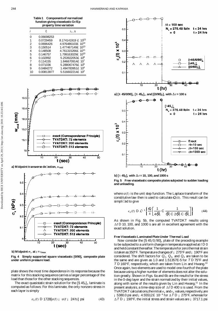
and ¾x at z D zmax using 72, 200, and 512 elements with 1t D 0:1 sare shown in Fig. 4, along with exact values computed by apply-ing the correspondenceprinciple. For the 200-elementmesh, using1t D 0:01 s did not signi� cantly change the results. The TVATDKTresults appear to converge to the exact solution.

Free Viscoelastic Laminated Plate Under Edge LoadThe plate dimensions are 1:0 £ 2:0 in. Each layer has a thickness

of 0.02 in.with the followingmaterial properties(matchinga Gr/Ep)at the instant the plate is loaded:

E1 D 18 Msi; G12 D 0:9 Msi; ®1 D 0:2 £ 10¡6=±F

(41)

E2 D 1:4 Msi; º12 D 0:34; ®2 D 16:0 £ 10¡6=±F

Once again, E1 is taken as � ber-dominated and constant in time.Hence, Q1 also will be constant in time. The other Qr then arecomputed as

Qr .t/ D Qr .0/ f .t/ where f .t/ D f0 C10

i D 1

fi e¡t=¸i .42/

The values given in Table 1 for fi and ¸i are those listed by Lin andHwang,10 which are a data � t to relaxationdata presented by Cross-man et al.2 A uniform edge load of Nx D 276:48 lb/in. is applied att D 0 and held constant until t D 24 h, at which point it is suddenlyremoved.

Because of symmetry, only one-fourth of the plate is analyzedusing two elements. The quasistatic strain results for several stack-ing sequences ([§45/0/90]s , [§452]s , and [.0=90/2]s ) are shown inFig. 5a for 1t D 100 s. As expected for this loading, the [§452]s

Dow

nloa

ded

by R

ICE

UN

IVE

RSI

TY

on

Apr

il 29

, 201

3 | h

ttp://

arc.

aiaa

.org

| D

OI:

10.

2514

/2.6

96

244 HAMMERAND AND KAPANIA

Table 1 Components of normalizedfunction giving viscoelastic Gr/Ep

property time variation

i fi ¸i , s

0 0.066982531 0.0729459 8.174141919 £ 1015

2 0.0696426 4:976486103£ 1014

3 0.150514 1:477467149£ 1013

4 0.148508 4:761315266£ 1011

5 0.146757 1:799163029£ 1010

6 0.102892 5:253922053£ 108

7 0.114155 1:846670914£ 107

8 0.071036 5:288067476£ 105

9 0.0484272 1:494783951£ 104

10 0.00813977 5:516602214£ 102

a) Midpoint transverse de� ection, wmid

b) Midpoint x at z = zmax

Fig. 4 Simply supported square viscoelastic [0/90]s composite plateunder uniform pressure load.

plate shows the most time dependence in its response because thematrix for this stacking sequence carries a larger percentage of theload than those for the other stacking sequences.

The exact quasistatic strain solution for the [§452]s laminate iscomputed as follows: For this laminate, the only nonzero stress ineach layer is simply

¾x .t/ D 1728[u.t/ ¡ u.t ¡ 24 h/] psi .43/

a) [§§ 45/0/90]s, [§§ 452]s, and [(0/90)2]s with D t = 100 s

b) [§ 452]s with D t = 10 100, and 1000 s

Fig. 5 Free viscoelastic composite plates subjected to sudden loadingand unloading.

where u.t/ is the unit step function. The Laplace transform of theconstitutive law then is used to calculate O²x .s/. This result can besimpli� ed to give

²x .t/ D ¡1 O¾x

s

1

4 OQ4

C 1OQ1 C 2 OQ2 C OQ3

.44/

As shown in Fig. 5b, the computed TVATDKT results using1t D 10; 100, and 1000 s are all in excellent agreement with theexact solution.

Free Viscoelastic Laminated Plate Under Thermal LoadNow consider the [§45=0=90]s plate of the preceding example

to be subjected to a uniform change in temperature applied at t D 0and held constant thereafter.The temperature for zero thermal strainis taken as 350±F. Temperature changes of ¡275±F and ¡190±F areconsidered. The shift factors for Q2, Q3, and Q4 are taken to bethe same and are given as 1.0 and 1.51357E-5 for T D 75±F andT D 160±F, respectively, which are taken from Lin and Hwang.10

Once again, two elements are used to model one-fourthof the platebecause using a higher number of elements does not alter the solu-tion greatly. Shown in Figs. 6a and 6b are the results for the stressin the 0-deg layer and the strain normalized by their initial values,along with some of the results given by Lin and Hwang.11 In thepresent analysis, a time-step size of 1t D 400 s is used. From theTVATDKT calculations,the initial¾x and ²x values,respectively,are¡5380:0 psi and ¡4:55512£ 10¡4 for 1T D ¡275±F, whereas for1T D ¡190±F, the initial stress and strain values are ¡3717:1 psi

Dow

nloa

ded

by R

ICE

UN

IVE

RSI

TY

on

Apr

il 29

, 201

3 | h

ttp://

arc.

aiaa

.org

| D

OI:

10.

2514

/2.6

96

HAMMERAND AND KAPANIA 245

a) Normalized x in 0-deg layer

b) Normalized x

Fig. 6 Free viscoelastic [§ 45/0/90]s plate subjected to uniform D Tapplied at t = 0 and held constant thereafter.

and¡3:14717£ 10¡4 , respectively.Lin and Hwang11 computedini-tial stress values of ¡5380 psi and ¡3717 psi for 1T D ¡275±Fand 1T D ¡190±F, respectively, with an initial strain value of¡4:56 £ 10¡4 for 1T D ¡275±F. Good agreement exists betweenthe present and previously published results. Finally, it is observedthat the thermorheologically simple viscoelastic response of theplate is a nonlinear function of the plate’s temperature.

Viscoelastic Composite Cylindrical Panels Under Pressure LoadTwo cylindrical panels differing only in the panel half-angle are

subjected to a uniform pressure load q0 D 0:3 psi, which is appliedsuddenly at t D 0 and held constant thereafter. The length of bothpanels is 80 in. and the arc length of the other side is either 41.89or 62.83 in., corresponding respectively to half-angles of Á D 12and 18 deg and a radius of 100 in. On each edge, both cylindricalpanels rest on diaphragms that are rigid in their plane but perfectly� exible otherwise. The cross-ply stacking sequence is [0=90]s withthe thicknessof each layer takento be0.08 in., givinga total laminatethickness of 0.32 in. The properties at the initial time match thosegiven in Eq. (41) for a Gr/Ep. Once again, Q1 is assumed to be � berdominated and constant in time. However, the Q2 – Q4 relaxationfunctions are determined from25

E2.t/ D .116:333 C 6:02203e¡t=287:154 C 10:8854 e¡t=5512:77

C 6:75662e¡t=113;384/ £ 104 psi (45)

G12.t/ D .75:9301 C 3:86299e¡t=287:154 C 6:3555 e¡t=5512:77

C 3:85226e¡t=113;384/ £ 104 psi (46)

where t is in minutes.A closed-form solution for this problem using shallow shell the-

ory is computed as follows. Let v1 , v2 , and v3 be the translationaldisplacements in the direction of the three shell coordinates. The� rst shell coordinate »1 varies along the direction having zero cur-vature,whereasthe secondshellcoordinate»2 varies along thedirec-tion having constant nonzero curvature. The third shell coordinate»3 (the shell normal) is determined from the right-hand rule andpoints away from the center of curvature of the »1-constant arcs. Aschosen, the shell coordinates are principal coordinates. Using theLove–Kirchhoff hypothesis and other approximations appropriatefor thin elastic laminated shallow shells as described by Leissa andQatu,26 the governingequations in terms of v1 , v2 , and v3 for a shal-low elastic cylindrical panel with a symmetric cross-ply stackingsequence under uniform pressure are

A11v1;11 C A12[v2;12 C .v3;1=R2/] C A66.v1;22 C v2;12/ D 0 (47)

A12v1;12 C A22[v2;22 C .v3;2=R2/] C A66.v1;12 C v2;11/ D 0 (48)

A12.v1;1=R2/ C A22 .v2;2=R2/ C v3 R22 C D11v3;1111

C 2.D12 C 2D66/v3;1122 C D22v3;2222 D q3 (49)

Here R2 is the radius associated with the panel and .¢/;i denotesdifferentiationwith respect to shell coordinate »i .

The uniform pressure load q3 is written as

q3 D q0 D1

m D 1;3;5

1

n D 1;3;5

16q0

¼ 2mnsin

m¼»1

l1sin

n¼»2

l2.50/

The boundary conditions are

»1 D 0; l1 : v2 D v3 D 0 and N11 D 0; M11 D 0

(51)

»2 D 0; l2 : v1 D v3 D 0 and N22 D 0; M22 D 0

(52)

where Ni j and Mi j are the usual force and force-couple resultants.Using the constitutivelaw, the strain-displacementrelationsand theconditions on v1 –v3 given above, the boundary conditions can bewritten strictly in terms of v1–v3 as

»1 D 0; l1 : v2 D v3 D 0 and v1;1 D 0; v3;11 D 0

(53)

»2 D 0; l2 : v1 D v3 D 0 and v2;2 D 0; v3;22 D 0

(54)

The boundary conditions and governing equations are satis� edexactly by the following Fourier series expansions:

v1 D1

m D 1;3;5

1

n D 1;3;5

Imn cosm¼»1

l1sin

n¼»2

l2

(55)

v2 D1

m D 1;3;5

1

n D 1;3;5

Jmn sinm¼»1

l1cos

n¼»2

l2

(56)

v3 D1

m D 1;3;5

1

n D 1;3;5

Kmn sinm¼»1

l1sin

n¼»2

l2

(57)

The constant coef� cients Imn ; Jmn , and Kmn for the elastic case aredetermined by substituting Eqs. (55), (56), and (57) into Eqs. (47),(48), and (49) and solving. The viscoelastic results then are com-puted using the correspondenceprinciple by replacing Ai j and Di j

with s OAi j .s/ and s ODi j .s/, respectively, and q0 with q0=s, and thentaking the inverse Laplace transform. A total of 49 Fourier terms isused to compute the shallowshell theory results,with the results for

Dow

nloa

ded

by R

ICE

UN

IVE

RSI

TY

on

Apr

il 29

, 201

3 | h

ttp://

arc.

aiaa

.org

| D

OI:

10.

2514

/2.6

96

246 HAMMERAND AND KAPANIA

a) Panel with 12-deg half-angle

b) Panel with 18-deg half-angleFig. 7 Midpoint transverse de� ection (v3)mid for viscoelastic [0/90]scylindrical panels subjected to a step uniform pressure load.

.v3/mid at t D 0 for the Á D 12-deg and Á D 18-deg panels, respec-tively, being slightly less than 0.007% and 0.12% different than theresults computed using 100 Fourier terms.

For both panels, a time-step size of 1t D 100 min is used. Thetime history of the midpoint de� ection for the Á D 12-deg panel isshown in Fig. 7a for several mesh sizes. The convergence appearsto be reasonable, with the error remaining for the 1800-elementcase approximately equal to ¡0:6% for large t. Shown in Fig. 8 areplots of the closed-form and 1800-element TVATDKT results forthe v3 de� ection at »1 D x D 0:5 l1 for t D 100 min and t D 600 h.The deformationpattern is such that a single extremum exists at thepanel center.

The cylindrical panel with the 18-deg half-angle is discretizedusing 1800 elements. The original undeformed mesh is shown inFig. 9a, whereas the deformedmesh at t D 600 h is shown in Fig. 9b.To ascertain the deformationpattern, the displacementswere scaledby a factor of 300 in Fig. 9b. Note that, when »2 D 0:5 l2 , the shellcoordinatesystemis alignedwith the x-y-z globalcoordinatesystemshown in Figs. 9a and 9b.

Shown in Figs. 10a and 10b are plots of the shallow shell the-ory and TVATDKT values for the v3 de� ection for the section at»1 D x D 0:5 l1 for t D 100 min and t D 600 h, respectively.As timeevolves, the v3 deformationstend to increase as the shell undergoescreep deformations,which can be observed by comparing Figs. 10aand 10b. Figure 7b shows the TVATDKT and shallow shell theoryresults for the time history of the transverse de� ection at the shell

Fig. 8 Transverse de� ection v3 at panel midsection ( 1 = 1/2l1) of aviscoelastic [0/90]s cylindrical panel with 12-deg half-angle subjectedto a step uniform pressure load. Results are shown for t = 100 min andt = 600 h.

a)

b)Fig. 9 Viscoelastic [0/90]s cylindrical panel with 18-deg half-anglesub-jected to step uniform pressure: a)undeformed mesh, b) deformed meshat t = 600 h with displacements multiplied by 300.

midpoint .v3/mid . The deformed shape of the shell at any given timeis similar to that shown in Fig. 9b. The applied pressure causes thetwo »2-constantedges to be pulled toward the panel center, whereasthe two »1-constant edges are pushed away from the panel center,but to a lesser extent. Because of the applied boundary conditions,the four corners do not translate. The two peaks in the deformationmove slightly inward as time evolves, whereas the center troughremains stationary because of symmetry. The differences betweenthe shallow shell theory and � nite element results for this panel aresomewhat larger than those for the Á D 12-deg panel for severallikely reasons. First, using 1800 elements for the Á D 18-deg panelgives a slightly larger element size than using 1800 elements forthe Á D 12-deg panel. Second, the adequacy of shallow shell theoryfor this problem decreases as the shell becomes deeper, i.e., as thepanel half-angle increases. Finally, the deformationpattern is morecomplex for the Á D 18-deg panel than for the Á D 12-deg panel.

Dow

nloa

ded

by R

ICE

UN

IVE

RSI

TY

on

Apr

il 29

, 201

3 | h

ttp://

arc.

aiaa

.org

| D

OI:

10.

2514

/2.6

96

HAMMERAND AND KAPANIA 247

a) t = 100 min

b) t = 600 hFig. 10 Transverse de� ection v3 at panel midsection ( 1 = 1/2l1 ) of aviscoelastic [0/90]s cylindrical panel with 18-deg half-anglesubjected toa step uniform pressure load.

Summary and ConclusionsThe geometrically linear dynamic analysis capability of an elas-

tic � at shell element has been extended to include thermoviscoelas-ticity. The element is the combination of the DKT plate bendingelement and a membrane element similar to the AT element, butderived by transferring the midside translationsof the LST elementto corner node translations and rotations. Prony series are used torepresent the relaxation moduli for linearly viscoelastic behavior,whereas reducedtimescalesare used to model hygrothermorheolog-ically simple materials. The hygrothermalloads also are included inthe formulation. Recursion relationships are employed to evaluatethe resultinghereditary integrals,and the Newmark time integrationscheme is implemented to incorporate inertial effects.

The results produced using the present formulation agreed wellwith solutions determined using the correspondenceprinciple andresults available in the existing literature for mechanical loads, ther-mal loads, and load removal. For the case of a cantilever under atip load, the dynamic results from the present formulation matchedthe results obtained from an independent viscoelastic plane-frameelement code developed by the present authors.

AcknowledgmentsDaniel Hammerand was supported during this research by a Na-

tional Science Foundation Graduate Research Fellowship. The sup-port for Rakesh Kapaniaduring this researchwas providedby GrantDAAH04-95-1-0175 from the Army Research Of� ce with GaryAnderson as the grantmonitor and is greatly appreciated.We wouldlike to thank Bernard Grossman, Department Head, Aerospace andOcean Engineering, for providing considerable computational re-sources. We would also like to thank Raymond Plaut, Departmentof Civil and Environmental Engineering, and P. Mohan and JingLi, Department of Aerospace and Ocean Engineering, for valuablediscussions held during the course of this research.

References1Aklonis, J. J., and MacKnight, W. J., Introduction to Polymer Viscoelas-

ticity, 2nd ed., Wiley, New York, 1983.2Crossman, F. W.,Mauri,R. E., and Warren, W. J., “Moisture-Altered Vis-

coelastic Response of Graphite/Epoxy Composites,” Advanced CompositeMaterials—Environmental Effects, STP 658, American Society for Testingand Materials, Philadelphia, PA, 1978, pp. 205–220.

3Lee, E. H., and Rogers, T. G., “Solution of Viscoelastic Stress Analy-sis Problems Using Measured Creep or Relaxation Functions,” Journal ofApplied Mechanics, Vol. 30, No. 1, 1963, pp. 127–133.

4Zak, A. R., “Structural Analysis of Realistic Solid-PropellantMaterials,”Journal of Spacecraft and Rockets, Vol. 5, No. 3, 1967, pp. 270–275.

5White, J. L., “Finite Elements in Linear Viscoelasticity,” Proceed-ings of 2nd Conference on Matrix Methods in Structural Mechanics, U.S.Air Force Flight Dynamics Lab., AFFDL-TR-68-150, Wright–PattersonAFB, Dayton, OH, 1968, pp. 489–516.

6Taylor, R. L., Pister, K. S., and Goudreau, G. L., “ThermomechanicalAnalysis of Viscoelastic Solids,” InternationalJournal for Numerical Meth-ods in Engineering, Vol. 2, No. 1, 1970, pp. 45–59.

7Wang, Y. Z., and Tsai, T. J., “Static and Dynamic Analysis of a Vis-coelastic Plate by the Finite Element Method,” Applied Acoustics, Vol. 25,No. 2, 1988, pp. 77–94.

8Ben-Zvi, R., “A Simple Implementation of a 3D Thermo-ViscoelasticModel in a Finite Element Program,” Computers and Structures, Vol. 34,No. 6, 1990, pp. 881–883.

9Krishna, A., Harper, B. D., and Lee, J. K., “Finite Element ViscoelasticAnalysis of Temperature and Moisture Effects in Electronic Packaging,”Journal of Electronic Packaging, Vol. 117, No. 3, 1995, pp. 192–200.

10Lin, K. Y., and Hwang, I. H., “Thermo-Viscoelastic Response ofGraphite/Epoxy Composites,” Journal of Engineering Materials and Tech-nology, Vol. 110, No. 2, 1988, pp. 113–116.

11Lin, K. Y., and Hwang, I. H., “Thermo-Viscoelastic Analysis of Com-posite Materials,” Journal of Composite Materials, Vol. 23, June 1989, pp.554–569.

12Hilton, H., and Yi, S., “Dynamic Finite Element Analysis of Viscoelas-tically Damped Composite Structures,” Applications of Supercomputers inEngineering II, edited by C. A. Brebbia, D. Howard, and A. Peters, Compu-tational Mechanics Publications, Elsevier Applied Science, London, 1991,pp. 495–511.

13Yi, S., and Hilton,H., “DynamicFiniteElement AnalysisofViscoelasticComposite Plates in the Time Domain,” InternationalJournal for NumericalMethods in Engineering, Vol. 37, No. 23, 1994, pp. 4081– 4096.

14Yi, S., Ahmad, M. F., and Ramesh, A., “Data Parallel Computationfor Thermo-Viscoelastic Analysis of Composite Structures,” Advances inEngineering Software, Vol. 27, No. 1–2, 1996, pp. 97–102.

15Lin, K. Y., and Yi, S., “Analysis of Interlaminar Stresses in ViscoelasticComposites,” InternationalJournal of Solids and Structures, Vol. 27, No. 7,1991, pp. 929–945.

16Yi, S., and Hilton,H., “Hygrothermal Effects on Viscoelastic Responsesof Laminated Composites,” Composites Engineering, Vol. 5, No. 2, 1995,pp. 183–193.

17Kapania, R. K., and Mohan, P., “Static, Free Vibration and Ther-mal Analysis of Composite Plates and Shells Using a Flat TriangularShell Element,” Computational Mechanics, Vol. 17, No. 5, 1996, pp. 343–

357.18Batoz, J. L., Bathe, K. J., and Ho, L. W., “A Study of Three-Node

Triangular Plate Bending Elements,” International Journal for NumericalMethods in Engineering, Vol. 15, No. 12, 1980, pp. 1771–1812.

19Allman, D. J., “A Compatible Triangular Element Including VertexRotations for Plane Elasticity Analysis,” Computers and Structures, Vol. 19,No. 1–2, 1984, pp. 1–8.

20Ertas, A., Krafcik, J. T., and Ekwaro–Osire, S., “Performance of anAnisotropic Allman/DKT 3-Node Thin Triangular Flat Shell Element,”Composites Engineering, Vol. 2, No. 4, 1992, pp. 269–280.

21Cook, R. D., “On the Allman Triangle and a Related QuadrilateralElement,” Computers and Structures, Vol. 22, No. 6, 1986, pp. 1065–1067.

22Reddy, J. N., An Introduction to the Finite Element Method, 2nd ed.,McGraw–Hill, New York, 1993.

23Christensen, R. M., Theory of Viscoelasticity, An Introduction, 2nd ed.,Academic, New York, 1982.

24Wolfram, S., The Mathematica Book, 3rd ed., Cambridge Univ. Press,New York, 1996.

25Marques, S. P. C., and Creus, G. J., “Geometrically Nonlinear FiniteElement Analysis of Viscoelastic Composite Materials Under Mechanicaland Hygrothermal Loads,” Computers and Structures, Vol. 53, No. 2, 1994,pp. 449–456.

26Leissa, A. W., and Qatu, M. S., “Equations of Elastic Deformationof Laminated Composite Shallow Shells,” Journal of Applied Mechanics,Vol. 58, No. 1, 1991, pp. 181–188.

A. M. WaasAssociate Editor

Dow

nloa

ded

by R

ICE

UN

IVE

RSI

TY

on

Apr

il 29

, 201

3 | h

ttp://

arc.

aiaa

.org

| D

OI:

10.

2514

/2.6

96