Thermosiphon Loops for Heat Extraction from the Ground

J U L I A R U D O R F

Study Project Stockholm, Sweden 2008

Thermosiphon Loops for Heat Extraction from the Ground

Julia Rudorf

Study Project Energy Technology 2008:451 KTH School of Industrial Engineering and Management Division of Applied Thermodynamic and Refrigeration

SE-100 44 STOCKHOLM

Study Project EGI 2008/ETT:451

Thermosiphon Loops for Heat Extraction from

the Ground

Julia

Rudorf Approved

27th March 2008 Examiner

Prof. Björn Palm Supervisor

José Acuna Commissioner

Contact person

Kenneth Weber, ETM Kylteknik

1

ABSTRACT

Ground source heat pumps use the energy from the ground for heating and cooling applications in buildings. This mechanism is carried out in a borehole in which a fluid circulates through a closed loop. In thermosiphon loops, the fluid circulates naturally while taking up the heat from the surrounding ground. The advantage of the natural circulation is that it substitutes the need of a circulating pump and this leads to a reduction of electricity consumption. Furthermore, in the case of leakage, ground water is not polluted because of being able to use natural fluids instead of traditional non-freezing fluids.

The project consists of two main parts, a theoretical and an experimental section. In the theoretical part a general literature survey is carried out, to sum up how technology concerning thermosiphon loops and heat extraction from the ground developed over the years and what is the state of the art. Subsequent to that, the experimental part follows with temperature measurements from a 70m deep vertical borehole with CO2 as refrigerant. The borehole heat exchanger is made of copper and it is composed of a central insulated pipe and a return line in spiral form. The results show that no natural circulation has been achieved and proposals for improvements and future work are pointed out.

2

ACKNOWLEDGEMENTS I would like to thank a number of people who helped and supported me during the process of this work. First of all, I wish to thank my supervisor José Acuna for his help and support during my stay at the Department of Energy Technology, Royal Institute of Technology, Stockholm. Furthermore, I would like to thank Professor Lothar Oellrich who has made the study abroad possible. Moreover, thanks to Professor Björn Palm and Dr Rahmatollah Khodabandeh for allowing me to participate in that interesting thermosiphon project. Special thanks to PhD student Carola Hölzer for correcting the theoretical part of the written paper. I also want to thank my family for always supporting me both financially as well as emotionally. Finally, special thanks to my friend Tiziana for her help, correction of the thesis and her useful comments, and also many thanks to Michi for always cheering me up and encouraging me during the last few months.

3

TABLE OF CONTENTS ABSTRACT .................................................................................................. 1 

ACKNOWLEDGEMENTS ............................................................................ 2 

TABLE OF CONTENTS ............................................................................... 3 

LIST OF SYMBOLS ..................................................................................... 5 

TABLE OF FIGURES ................................................................................... 7 

TABLE OF TABLES ..................................................................................... 8 

1. INTRODUCTION ...................................................................................... 9 

1.1 Geothermal Heat .................................................................................9 

1.2 Advantages of Ground Heat ..............................................................10 

1.3 Other Types of Heat Sources for Heat Pumps ..................................10 

1.4 Ground-Coupled Heat Pumps ...........................................................11 

1.5 General Design of Ground Source Heat Pumps ...............................13 1.5.1 Open Loops.................................................................................................. 13 1.5.2 Closed Loops ............................................................................................... 14 1.5.3 Vertical System ............................................................................................ 16 

1.5.3.1 Advantages of Vertical Installations ........................................................ 16 1.5.3.2 Disadvantages of Vertical Installations ................................................... 16 

1.6 Applications and General Technical Data in Sweden .......................16 

1.7 Borehole Heat Exchanger .................................................................18 1.8 Guidelines .........................................................................................19 1.9 Damages on GSHP ...........................................................................19 

2. OBJECTIVES ......................................................................................... 20 

3. THERMOSIPHON LOOPS ..................................................................... 20 

3.1 Mechanism of Thermosiphon ............................................................20 

3.2 Advantages of Thermosiphon ...........................................................21 

3.3 Disadvantages of Thermosiphon .......................................................21 

3.4 General Design of Thermosiphon .....................................................22 

3.5 Thermosiphon Properties ..................................................................23 3.5.1 Flooding Limit in Thermosiphon Pipe ....................................................... 23 3.5.2 Refrigerant Fluids ........................................................................................ 24 

3.5.2.1 CO2 ......................................................................................................... 25 3.5.2.2 History of CO2 ......................................................................................... 27 3.5.2.3 Advantages of CO2 ................................................................................. 27 3.5.2.4 Disadvantages of CO2............................................................................. 28 

3.5.3 Materials for Heat Pipes .............................................................................. 28 3.5.4 Rate of Heat Transfer .................................................................................. 29 3.5.5 Diameter ....................................................................................................... 30 3.5.6 Borehole Depth ............................................................................................ 31 3.5.7 Pressure Drop for Thermosiphon Pipe ...................................................... 31 3.5.8 Temperature Distribution ............................................................................ 32 3.5.9 Film Thickness ............................................................................................. 34 3.5.10 Velocity ....................................................................................................... 34 3.5.11 Final Design ............................................................................................... 35 

4. DESCRIPTION OF INSTALLATION AND EXPERIMENTAL SET UP ... 36 

4.1 Test Rig Setup...................................................................................36 4.1.2 Components of Test Rig ............................................................................. 36 

4

4.1.3 Principal Design of Test Rig ....................................................................... 37 4.1.4 Measurement Instruments .......................................................................... 40 4.1.5 The Setup and Installation Process ........................................................... 41 

4.2 Previous Calculations ........................................................................42 4.2.1 Pressure Drop .............................................................................................. 42 4.2.2 Filling Rate ................................................................................................... 44 

4.3 Planned Measurements ....................................................................44 

4.4 Testing Method..................................................................................45 4.5 Occurrence of Difficulties during the Installation Process .................46 

4.6 Modification of Design .......................................................................46 

5. DISCUSSION OF RESULTS ................................................................. 47 

5.1 Undisturbed Ground ..........................................................................47 5.1.1 Temperature Sensors .................................................................................. 47 5.1.2 Optical Fibre................................................................................................. 48 5.1.3 Comparison and Discussion ...................................................................... 50 

5.2 Results with the System in Operation - First Design .........................50 

5.3 Results with the System in Operation – Modified Test Rig ...............52 5.3.1 Temperature Sensors .................................................................................. 52 5.3.2 Optical Fibre................................................................................................. 54 5.3.3 Comparison and Discussion ...................................................................... 57 

6. CONCLUSIONS ..................................................................................... 57 

7. PROBLEMS AND RECOMMENDATIONS ............................................ 58 

8. SUMMARY AND OUTLOOK .................................................................. 59 

REFERENCES ........................................................................................60 Appendix A: Table of Chemical Data of CO2 ...........................................63 

Appendix B: Calculations of Pressure Drop ............................................63 

Appendix C: Calculations of Filling Rate .................................................65 

5

LIST OF SYMBOLS Abbreviations COP Coefficient of performance

SPF Seasonal performance

factor

GSHP Ground source heat pump

GCHP Ground coupled heat pump

GWHP Ground water heat pump

SWHP Surface water heat pump

CFC Chlorofluorocarbon

HCFC Hydrofluorocarbon

CO2 Carbon dioxide

R22 Chlordifluormethan

R134A Tetrafluorethan

R414A Refrigerant circulating in the heat pump

VDI DTS

Verein Deutscher Ingenieure (association of German engineers) Distributed Temperature Sensor

Standards p [bar] = [1*105 N/m2] Pressure h g f v

[m] [m/s2] [-] [m3/kg]

Height Gravity Coefficient of pressure drop Specific volume

w [m/s] Velocity L [m] Length D, d [m] Diameter G [kg/m2s] Mass flow rate V [m3] Volume k [W/mK] Thermal conductivity m& [kg/s] Mass flow A [m2] Area Q& [W] = [J/s] Heat flux

6

x [-] Ratio of liquid / gas h [J/kg] Enthalpy Greek symbols ρ [kg/m3] Density η [Ns/m2] Dynamic viscosity ν [m2/s] Kinematic viscosity Dimensionless numbers Re [-] Reynolds Number

7

TABLE OF FIGURES Fig. 1: Classification of Ground Zones [8] ...................................................................... 10 Fig. 2: Annual Sale of GSHP in Sweden [20] ................................................................. 12 Fig. 3: Annual Sale of GSHP in Germany [7] ................................................................. 12 Fig. 4: Ground Water Heat Pump [15] ........................................................................... 14 Fig. 5: Glycol-and water Ground Source Heat Pump [15] .............................................. 14 Fig. 6: Horizontally Installed Pipes [15] .......................................................................... 15 Fig. 7: Horizontally Installed Systems [8] ....................................................................... 15 Fig. 8: Self-circulating GSHP [15] .................................................................................. 16 Fig. 9: Temperature Distribution in Sweden ................................................................... 17 Fig. 10: Typical Conditions in Sweden [20] .................................................................... 18 Fig. 11: Different Types of Borehole Heat Exchangers [20] ........................................... 19 Fig. 12: Thermosiphon Mechanism [6] .......................................................................... 21 Fig. 13: Reversal Heat Input [15] ................................................................................... 22 Fig. 14: Different Designs of Thermosiphon Loops ........................................................ 23 Fig. 15: Charge of CO2 against Evaporation Temperature [6] ....................................... 24 Fig. 16: Phase Diagram of CO2 [9] ................................................................................ 25 Fig. 17: h-logp Diagram of CO2 [Refprof] ....................................................................... 26 Fig. 18: Vapour Pressure of Different Refrigerants [9] ................................................... 26 Fig. 19: Historical Development of Refrigerants [27] ..................................................... 27 Fig. 20: Temperature Difference against Heat Flux for Different Refrigerants [15] ........ 30 Fig. 21: Pressure Profile in the Heat Pipe [15] ............................................................... 32 Fig. 22: Temperature Variation with Depth in Nicosia, Cyprus [8] ................................. 32 Fig. 23: Simulated Temperature Increase along the Tube [6] ........................................ 33 Fig. 24: Temperature-Time Curve for Different Depths [15] .......................................... 34 Fig. 25: Velocity Profile in the Thermosiphon Tube [11] ................................................ 35 Fig. 26: Number of Parallel Installed Thermosiphons [6] ............................................... 36 Fig. 27: Heat Pump Test Rig ......................................................................................... 37 Fig. 28: Experimental Test Rig ...................................................................................... 38 Fig. 29: Thermosiphon Loop First Version……………………………………………...…..39 Fig. 30: Dimensions of the Thermosiphon ..................................................................... 39 Fig. 31: Specific Dimensions of the Test Rig ................................................................. 40 Fig. 32: Arrangement of the Thermosiphon Loop .......................................................... 40 Fig. 33: Optical Fibre [DTS Manual] .............................................................................. 41 Fig. 34: Location of Temperature Sensors .................................................................... 45 Fig. 35: Modified Design of Thermosiphon Loop ........................................................... 46 Fig. 36: Undisturbed Ground, Temperature Sensors on the Pipe (5th-6th Feb.2008) ..... 47 Fig. 37: Undisturbed Ground, Temperature Sensors on the Borehole (5th-6th Feb.2008) ...................................................................................................................................... 47 Fig. 38: Undisturbed Ground, Temperature Sensors, Comparison (5th-6th Feb.2008) ... 48 Fig. 39: Undisturbed Ground, Optical Fibre (5th-6th Feb.2008) ....................................... 49 Fig. 40: Undisturbed Ground, Optical Fibre, Different Depth (5th-6th Feb.2008)............. 49 Fig. 41: Running Process, Temperature Sensors, Pipe (30th Jan.2008) ........................ 51 Fig. 42: Running Process, Temperature Sensors, Borehole (30th Jan.2008) ................ 52 Fig. 43: Modified Running Process, Temperature Sensors, Pipe (7th Feb.2008) ........... 53 Fig. 44: Modified Running Process, Temperature Sensors, Borehole (7th Feb.2008) .... 53 Fig. 45: Stabilisation of the System, Temperature Sensors (7th Feb.2008) ................... 54 Fig. 46: Modified Running Process, Optical Fibre (7th Feb.2008) .................................. 55 Fig. 47: Comparison Modified Running Process and Undisturbed Ground, Optical Fibre (7th Feb. 2008) ............................................................................................................... 55 Fig. 48: Modified Running Process, Optical Fibre (7th Feb. 2008 (1)) ............................ 56 

8

Fig. 49: Modified Running Process, Optical Fibre (14th Feb. 2008 (2)) .......................... 57 

TABLE OF TABLES Table 1: Quantity of Sold GCHP Units 2005 [20] ........................................................... 11 Table 2: COP Values for Different Types of Heat Pipe [28] ........................................... 13 Table 3: Material Removal Test [21] .............................................................................. 29 

9

1. INTRODUCTION Renewable energy is a kind of energy that derives from natural resources which are inexhaustible. The International Energy Agency declares that “renewable energy is derived from natural processes that are replenished constantly. In its various forms, it derives directly from the sun or from heat generated deep within the earth”. [IEA Renewable Working Party, “Renewable Energy…into the Mainstream”] [1] This includes mainly solar light, solar heat, wind power, geothermal heat, water power and biomass. Renewable energy will substitute fossil fuel resources for the long term or - at present - at least reduce the dependency on fossil fuels. In addition to that, it will lead to a reduction of greenhouse gases. 1.1 Geothermal Heat Geothermal heat or ground heat ranks among nearly infinite renewable energy. The geothermal potential is inexhaustible and has a large thermal inventory. Its application varies from electric power generation to district heating. Moreover, it serves for heating and cooling of buildings such like small and big residential and commercial houses. The technology of ground source heat pumps profits from geothermal heat and from the capacity of the sun to load the ground with heat. In particular, heating is one of the basic needs of humanity. Geothermal energy offers heat and power. According to Propiel et al. the ground can be classified into three main zones [8]:

1. Surface zone: the average depth is about 1m. This implicates that the ground temperature is very sensitive to short time weather condition changes.

2. Shallow zone: the depth ranges from 1m to 8m for dry light soils alternatively 20m for most heavy sandy soils. Characteristic for that zone is that the ground temperature is nearly constant during the year and only minimal changes occur during seasonal weather condition changes.

3. Deep zone: ground temperatures that are nearly independent of changes in weather conditions below 8m-20m.

Fig. 1 represents the different ground zones.

10

Fig. 1: Classification of Ground Zones [8] 1.2 Advantages of Ground Heat The advantage of ground heat is the constant ground temperature all over the year below a depth of approximately 5m-10m or even lower, independent of weather conditions [2]. In [8] it is mentioned that “temperature fluctuations at the surface of the ground are diminished as the depth of the ground increases because of the high thermal inertia of the soil.” In addition ground heat is infinite and available all over the world and free of charge. 1.3 Other Types of Heat Sources for Heat Pumps The heat source is of vital importance for the cost-effectiveness, for the environmental effects as well as for the technological efficiency of heat pump systems [13]. Which kind of heat source is used for the corresponding application depends on the size of the geothermal system. Small systems, e.g. family houses, use diverse heat sources such as ambient air, exhaust air, lake or river water, soil, rock. In large installations water is selected as heat source, mainly lake water as well as cleaned sewage water. The influence of the heat source on the choice of the working fluid is negligible or small [13]. Ambient air and exhaust air have an excellent availability but their temperature levels can be low in contrast to other heat sources due to high temperature fluctuations during the year because of seasonal weather conditions [13]. Therefore, the coefficient of performance (COP) can be comparatively small (An explanation of COP will be given in section 1.4).

11

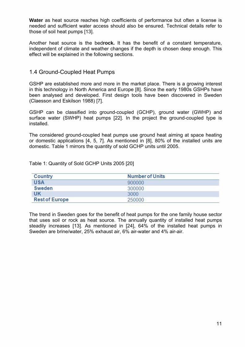
Water as heat source reaches high coefficients of performance but often a license is needed and sufficient water access should also be ensured. Technical details refer to those of soil heat pumps [13]. Another heat source is the bedrock. It has the benefit of a constant temperature, independent of climate and weather changes if the depth is chosen deep enough. This effect will be explained in the following sections. 1.4 Ground-Coupled Heat Pumps GSHP are established more and more in the market place. There is a growing interest in this technology in North America and Europe [8]. Since the early 1980s GSHPs have been analysed and developed. First design tools have been discovered in Sweden (Claesson and Eskilson 1988) [7]. GSHP can be classified into ground-coupled (GCHP), ground water (GWHP) and surface water (SWHP) heat pumps [22]. In the project the ground-coupled type is installed. The considered ground-coupled heat pumps use ground heat aiming at space heating or domestic applications [4, 5, 7]. As mentioned in [8], 80% of the installed units are domestic. Table 1 mirrors the quantity of sold GCHP units until 2005. Table 1: Quantity of Sold GCHP Units 2005 [20]

The trend in Sweden goes for the benefit of heat pumps for the one family house sector that uses soil or rock as heat source. The annually quantity of installed heat pumps steadily increases [13]. As mentioned in [24], 64% of the installed heat pumps in Sweden are brine/water, 25% exhaust air, 6% air-water and 4% air-air.

12

Fig. 2: Annual Sale of GSHP in Sweden [20]

Fig. 3: Annual Sale of GSHP in Germany [7]

Analysing the statistical data in Fig. 2 the number of sold ground source heat pumps in Sweden can be compared over the years since 1985. One can see the steady increase of sold systems over the year, except the number of sales in 1985 which includes all the units installed until that year. The trend in Fig. 3 shows that in Germany the sale of heat pumps has augmented more and more over the years as well. The sale in Sweden, represented in Fig. 2, constantly stays on a high level between 2003 and 2005, more than twice as high as in Germany, except in 2006. One possibility of comparing different kinds of heat pumps is the seasonal performance factor (SPF) or the coefficient of performance (COP). SPF describes the ratio of useful energy output of a device to the energy input, averaged over an entire heating season. COP means the ratio of the output heat to the supplied work at certain conditions. COP

13

will be meaningful if the conditions are equal. SPF as figure of merit will be reasonable if distinct regions with different conditions are compared. GCHPs normally reach higher COP/SPF values than other types of heat pumps because of the higher and more stable source temperature. That effect leads to a rising sale [2]. In [38] it is stated that GCHP systems represent higher COPs because of the better thermal properties of the soil/rock compared to conventional heat pumps. According to [2], a comparison of an air source pump with a GCHP has been done showing that the SPF is 2.5 for the former case while it has a value of 4 for the latter. The values depend on the climate conditions but GCHP normally have a higher SPF value. It follows from this, that GCHP are favored. The following table shows values of COP for different heat pumps. The air source type shows more fluctuations as result of weather conditions. For ground source heat pumps the COP values are more stable. Table 2: COP Values for Different Types of Heat Pipe [28]

Whereas GCHP can be used as cooling application in summer it can also operate as heating system in winter. It depends on the location whether the emphasis is put on heating or cooling. In colder areas the demand of heating is higher than in warmer climate zones. Nevertheless, there are some established commercial installations with big cooling loads even in Scandinavia [7]. 1.5 General Design of Ground Source Heat Pumps In general, the systems can be installed either horizontally, vertically or inclined [8]. This can be done in open and closed loops. It will merely be dwelled on rock as source for the heat pump. 1.5.1 Open Loops In an open loop the warmth of the ground is used directly, for example groundwater systems or pre-heating air systems, as follows:

• Groundwater heat pumps (Fig. 4): if groundwater is used as heat source for the heat pumps two standpipes will be required: one to extract the warm groundwater, a so-called withdrawal well, and one to recycle the used water back to the ground, a dry well. The warm water from the withdrawal well is pumped to the evaporator of the heat pump. After extracting the heat, the chilled water is pumped back to the ground [15].

14

Fig. 4: Ground Water Heat Pump [15]

1.5.2 Closed Loops In a closed loop the ground is used indirectly and a heat carrier medium as for example glycol-water GSHP, circulates through a borehole heat exchanger.

• Glycol- and water ground source heat pump (Fig. 5): precondition for this form of technology is one or even more boreholes in which pipes are installed. The residual space between the pipe and the surrounding is filled up with a dense material which main parameter is an excellent heat transfer medium. In Sweden, this material is commonly groundwater which is naturally found when drilling the hole. In each borehole one pipe is installed at least. The circulating fluid absorbs the ground heat and transports it to the heat pump.

Fig. 5: Glycol-and water Ground Source Heat Pump [15]

• Horizontally installed pipes (Fig. 6): another design of a heat extraction system

are horizontally installed pipes. That design requires a large amount of space [15].

15

Fig. 6: Horizontally Installed Pipes [15]

The pipes are buried in the ground at a depth of about 1-2m below the ground surface [2]. They are usually made of PE 100 [15]. In groundwater protection areas a special license is necessary [7].

Fig. 7: Horizontally Installed Systems [8]

As can be seen in Fig. 7 below, different designs are available: parallel, series, trench connections or other special designs. It will not be dwelled on advantages and disadvantages because a horizontal loop will not be realised in the experimental part.

• Self-circulating GCHP: This system is based on the mechanism of a

thermosiphon and the fluid circulates due to density differences which occur because of temperature changes [15]. The mechanism of the thermosiphon is illustrated below. Fig. 8 shows the general design which will be explained more precisely in chapter 3.

16

Fig. 8: Self-circulating GSHP [15]

1.5.3 Vertical System The design is that important because unlimited ground area is becoming more and more rarely [6]. Thus, that installation design will be chosen if a disruption of landscape shall be avoided and if a confined surface exists, such as a rocky one close to the surface [8]. There is also the possibility to arrange the pipe in inclined position to reduce the distance between different pipes. Vertical installations reach a depth of – depending on the author 50-150m [8] or even 250m [2]. There are also higher depths but not for the one family house sector. 1.5.3.1 Advantages of Vertical Installations In summary, three advantages can be emphasised. The vertical design requires less space and achieves less disruption of landscape as horizontal ones [2], [8]. Moreover, it offers constant soil temperatures almost all over the year independent of any weather climate changes [2]. Finally, it needs less piping material in comparison to horizontal installations [13]. 1.5.3.2 Disadvantages of Vertical Installations As disadvantages the need of the brine pump for overcoming the pressure drop [8] and its energy requirement should be mentioned. However, this pump can be eliminated if the mechanism of thermosiphon is involved in the installation. Furthermore, the installation is more expensive [8], especially because of the drilling costs. 1.6 Applications and General Technical Data in Sweden This subsection focuses in particular on the designs used in Sweden. Generally, the soil mainly consists of crystalline rock [7].

17

In Fig. 9 the temperature distribution in Sweden for a depth of 100m can be seen. In the Stockholm region it refers to 7ºC. This will be verified in the experimental part of this written paper.

Fig. 9: Temperature Distribution in Sweden

(Depth of 100m), (Signhild Gehlin Autovisual Material, VVS tekniska föreningen)

Typical Swedish parameters for GCHP are the following:

- Ground source temperature: 3-10 ºC, Stockholm: 7 ºC - Borehole depth: 150m - Borehole capacity: 7kW - System COP: 3,3 - Heat extraction rate: 40W/m - Ground loop temperature design: -3 / 0 °C - Heat pump technical life: 15-20 years - Borehole technical life: 30-50 years - Payback time 6-9 years

Those values are from an investigation of Göran Hellström, Lund University [20].

18

Fig. 10: Typical Conditions in Sweden [20]

In Sweden does not exist any special precondition for the planning of a GSHP system. In general, no legal permission is necessary unless it is planned in water protected areas or close to urban areas. However, there is a norm (NORMBRUNN 97) that must be followed and the borehole has to be reported [20]. For the borehole completion there exist several rules: a casing has to be fixed through the soil layer and 2m into the rock [20]. Moreover, in urban areas a neighbour agreement is required. In general, the installation costs are high but the lower operational costs compensate these first costs. 1.7 Borehole Heat Exchanger By choosing a closed loop system, a borehole heat exchanger (BHE) is needed. There are two different types: U-tube and coaxial design. U-tubes consist of two straight pipes linked with an U-turn at the bottom. That is displayed in Fig. 11. Normally they are made of polyethylene which is known for its chemical resistance and its durability [4], [7]. Coaxial pipes are more complex. The ordinary design is one straight pipe in another pipe that has a larger diameter [8] what can be seen in Fig. 11. The experimental part will refer to the coaxial case. That is explained precisely in chapter 4. The typical diameter of a BHE is 10-15cm for a depth of 20-300m for vertical installations. In one family houses in Switzerland a diameter of 10-15cm for a depth of 100-200m is a typical parameter for a borehole heat exchanger [8].

19

Fig. 11: Different Types of Borehole Heat Exchangers [20]

1.8 Guidelines The huge interest in ground source heat pump applications is attested in section 1.4. The increasing demand may imply that companies employ engineers who have no planning experience or enough appropriate training [7]. Thus, the huge request of ground source heat pumps entails a desire for standardised operations and special requirements for qualified work or dimensioning to avoid negative consequences for the environment [7]. Several guidelines for the development of GSHP are in use. In Germany, the guideline VDI (association of German engineers) 4640 is used. Part 1 and 2 exists in German and English. It describes the state of the art in planning, construction and dimensioning of GSHPs. Additionally a DIN (German industrial norm) standard with BHE drilling and installation instructions will be published soon. In Switzerland the SIA 384/6 exists and in France the NF X 10/999 is in use [7]. 1.9 Damages on GSHP Diverse damages on GSHP were noticed in the past. First damages can already happen during the installation process. The tube may be damaged and a leakage is the result [18]. If too much heat is extracted the system may break down due to a freezing incident around the pipe [18]. Moreover, the ground surface may be lifted during winter and in summer time it may slide because of the missing ice [18]. A very general problem is the under-dimensioning of the heat pipe which could lead to a collapse of the system. Furthermore, the heat transfer flux may be affected by bad or missing backfill of the heat pipe. In addition technical failures can occur [18].

20

2. OBJECTIVES The main objectives of the project were:

• Understand how thermosiphon loops for heat exchange with the ground operate

• Sum up state of the art information about thermosiphon loops for heat exchange with the ground

• Test and analyse a closed thermosiphon loop from a real borehole installation

• Point out potentials for system improvement and design suggestions for the

thermosiphon installation

3. THERMOSIPHON LOOPS Common GCHPs with vertically installed heat exchangers need a pump to circulate the fluid continually. Such a pump requires energy and therefore new concepts are developed to avoid the necessity of a circulating pump. Hence, a GCHP can be designed with the basic principle of the mechanism of thermosiphon where condensation and evaporation is repeated continuously [19]. Economical projects with thermosiphon mechanism were installed for the first time 2001/2002 [5]. 3.1 Mechanism of Thermosiphon It is explained above that the fluid in a heat pipe which works according to the thermosiphon mechanism circulates by itself. The liquid fluid takes up the heat from the ground and this leads to the evaporation of the fluid. Because of its less density the emerged vapour rises upwards. The denseness difference occurs because of a phase change. The impulse of that phase change is the temperature difference [19]. On the top of the pipe the temperature decreases due to heat extraction from the fluid and the fluid condenses. Due to gravity the condensed liquid trickles downwards on the wall. The liquid film is again heated up and the process continues as explained above. The process may be visualised as a counter current two-phase flow between the evaporator section and the condensing section if a gravity-assisted heat pipe is considered. For a thermosiphon consisting of two tubes or a thermosiphon loop, the flow can be seen as co-current. Fig. 12 explains the thermosiphon mechanism on the basis of a single-tube two-phase thermosiphon. The heat pipe can be divided into three sections [2]:

1. The part of the bottom of the heat pipe is called evaporation section. 2. The part in the middle of the heat pipe is named adiabatic section. 3. The section on the top of the heat pipe is called condensing section.

21

Fig. 12: Thermosiphon Mechanism [6]

3.2 Advantages of Thermosiphon Thermosiphon loops offer a lot of advantages. Generally, the aim of technologies is to optimise or to develop new systems which are cost-effective, working effective and harmless for the environment. Compared to other GSHP systems, thermosiphon technology presents an environmental protective method by using CO2 as refrigerant [2]. In case of a leakage there is no contamination of the groundwater. This form of self circulation does not need any pump and therefore reduces the electrical consumption [6]. Without a pump the risk of wear [10] of pump components is minimised and the operating costs [10] as well as the investment costs are lower [13]. Moreover, the durability of the system without an additional pump is extended [10]. The temperature drop may be small but nevertheless it can extract and transport a high heat rate [25]. The efficiency is described with a COP > 5 as indicated in [17]. 3.3 Disadvantages of Thermosiphon Beside a large list of advantages some negative facts have been noticed. The main disadvantage is that it does not work in cooling mode but only in heating mode because the condenser only works in one direction as said in [2]. In addition, the first costs, especially the drill, are very high. However, that is the case for every form of vertical heat pump. If it is a direct evaporation system the heat pump has to be designed fancier than in conventional systems. The evaporator has to be placed at the head of the loop. That means a splitting of the heat pump or a difference in altitude so that the condensed thermosiphon fluid is able to flow back to the bottom. Another possibility is an additional

22

pump that transports the condensed liquid back to the ground. This is not desired by reason of energy consumption. The disadvantage of unavailable cooling could be solved with another design idea that will be presented below [15]. 3.4 General Design of Thermosiphon In general, there are three different designs of GSHP with thermosiphon mechanism (see Fig. 14). In a one tube design of GSPH the two converse flows, vapour and liquid, may interact. This may lead to a dryout on the bottom of the pipe and limits the maximum heat flux considering thermosiphon pipes [15]. The other design is a two tube thermosiphon. There are two tubes and the inner one is equipped with a hopper on the top. It has been found out that in that arrangement (with a hopper on the top), the limit of heat transfer is 4.5 times better than in conventional thermosiphons. One explanation for that merit is that no interaction between vapour and liquid occurs. For this design a filling rate of 80% has been chosen for an optimal working. Above all, such a design offers the possibility of cooling [15]. According to [15], cooling can be realised in a separate circuit in which the GSHP works as condenser. In the cooling mode the heat pump is switched off and the compressor increases the pressure in the outer tube so that the liquid flows upwards in the inner tube. In the evaporator the cold is transferred to the circuit of the house. [15] One disadvantage that should be mentioned is the possibility that oil of the compressor may get into the circuit and may contaminate the ground water. A solution to that problem may be oil-free compressors. Costs and benefits should be considered carefully. Fig. 13 mirrors that design.

Fig. 13: Reversal Heat Input [15]

Furthermore, there exists a third alternative of design, a thermosiphon loop. It consists of a riser and a downcomer and the fluid evaporates at the bottom and condenses at the head of the loop. In current applications only one tube thermosiphons exist, a two-tube design could not become accepted yet. A thermosiphon loop for domestic heating has not been

23

sufficiently investigated yet and has not influenced the single-tube market yet. In the early 1990s some researchers compared the single-tube thermosiphon to the double-tube thermosiphon. These investigations showed that a double-tube thermosiphon could be 4.5 times more efficient than the single-tube thermosiphon if the filling rate is chosen favourable [26]. However, that experiment was a double-tube thermosiphon with a hopper on the top. Assumedly, the efficiency of a thermosiphon loop is similar to a double-tube thermosiphon. Nevertheless, in the current research no investigations of a spiral type loop which is utilised in the project and which is presented in chapter 4 could be found.

Fig. 14: Different Designs of Thermosiphon Loops 3.5 Thermosiphon Properties In the following, different parameters of thermosiphons are described. Because of the lack of research in thermosiphon loops it will also be dwelled on the single- and double-tube thermosiphons. Moreover, it is probable that also a counter-current flow happen in the test rig. 3.5.1 Flooding Limit in Thermosiphon Pipe Flooding is an appearance that may happen in thermosiphon applications. Precondition for flooding is that a counter-current flow occurs. Flooding takes place in case of a mismatch between the flow of vapour upwards and downwards trickling liquid [11]. Depending on the system dimensions, the heat flux is limited at special values. Parameters that define the critical heat flux are the probe length, the fluid properties and the diameter [3]. If that critical heat flux is exceeded the pipe will be flooded. An average value of heat extraction rate to which it can be geared is 50W/m. Nevertheless, attention to the special regional soil conditions should be paid. The vapour that flows upwards to the head of the probe is able to convert the direction of the downwards trickling liquid film. The two fluxes interact and on the surface shear stress may occur. If that happens, the evaporation section of the pipe will dry out due to the lack of liquid that is stored at the upper end of the pipe [3]. It is also possible that no dry out occurs but liquid may get in the gas flow because of temperature fluctuations.

24

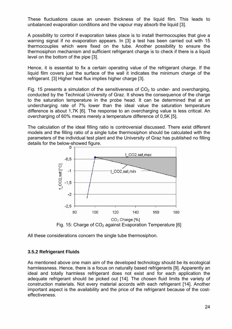
These fluctuations cause an uneven thickness of the liquid film. This leads to unbalanced evaporation conditions and the vapour may absorb the liquid [3]. A possibility to control if evaporation takes place is to install thermocouples that give a warning signal if no evaporation appears. In [3] a test has been carried out with 15 thermocouples which were fixed on the tube. Another possibility to ensure the thermosiphon mechanism and sufficient refrigerant charge is to check if there is a liquid level on the bottom of the pipe [3]. Hence, it is essential to fix a certain operating value of the refrigerant charge. If the liquid film covers just the surface of the wall it indicates the minimum charge of the refrigerant. [3] Higher heat flux implies higher charge [3]. Fig. 15 presents a simulation of the sensitiveness of CO2 to under- and overcharging, conducted by the Technical University of Graz. It shows the consequence of the charge to the saturation temperature in the probe head. It can be determined that at an undercharging rate of 7% lower than the ideal value the saturation temperature difference is about 1,7K [6]. The response to an overcharging value is less critical. An overcharging of 60% means merely a temperature difference of 0,5K [5]. The calculation of the ideal filling ratio is controversial discussed. There exist different models and the filling ratio of a single tube thermosiphon should be calculated with the parameters of the individual test plant and the University of Graz has published no filling details for the below-showed figure.

Fig. 15: Charge of CO2 against Evaporation Temperature [6]

All these considerations concern the single tube thermosiphon. 3.5.2 Refrigerant Fluids As mentioned above one main aim of the developed technology should be its ecological harmlessness. Hence, there is a focus on naturally based refrigerants [9]. Apparently an ideal and totally harmless refrigerant does not exist and for each application the adequate refrigerant should be picked out [14]. The chosen fluid limits the variety of construction materials. Not every material accords with each refrigerant [14]. Another important aspect is the availability and the price of the refrigerant because of the cost-effectiveness.

25

The influence of the heat source on the choice of the working fluid is negligible or small. Chlorofluorocarbon (CFC) and Hydrochlorofluorocarbons (HCFCs), for example R22, are refrigerants that were introduced in the 1930s. The utilization of CFCs has been interdicted in new applications because of the negative impact on the environment. In Sweden new applications using CFCs and HCFCs were abolished in 1998. Therefore, their use for thermosiphon applications will not be discussed. Ammonia has asserted itself on the market over many decades and has not been abolished by the introduction of freons in the 1930s. It has very good heat transfer properties but it is combustible and poisonous [14]. Furthermore it cannot be applied together with copper pipes because of corrosion [15]. Propane could also be utilized in thermosiphon applications but in some countries the public authority impedes their usage [16]. Another refrigerant that is frequently used in thermosiphon loops is CO2. Due to the great importance and the use of that refrigerant in the experiment, it is characterised in a separate section. 3.5.2.1 CO2 CO2 is a natural refrigerant that circulates in the biosphere [14]. The history of that refrigerant is described below. Fig. 16 demonstrates the phase diagram of CO2.

Fig. 16: Phase Diagram of CO2 [9]

Concerning the project the h-logp diagram of CO2 prove to be essential. Fig. 17 shows the h-logp diagram of CO2 in the range of the project-parameters. In Fig. 17 one can determine the temperature for a specified pressure and find out the corresponding gaseous state.

26

Fig. 17: h-logp Diagram of CO2 [Refprop]

CO2 is the refrigerant that is chosen in the majority of thermosiphon-cases. Its thermodynamic and transport properties are not comparable to other refrigerants, according to [9]. In this section the properties of CO2 will be compared to those of other refrigerants. As described above, CO2 offers a high vapour pressure compared to other refrigerants. But by increasing the pressure, the temperature value changes not as much because of the high gradient of the curve (Fig. 18)

Fig. 18: Vapour Pressure of Different Refrigerants [9]

The vapour density of CO2 is very high compared to other refrigerants. According to [5], it is 7 times higher as the vapour density of R134a. Moreover, CO2 offers good heat transfer characteristics. The thermal conductivity is 20% and 60% higher than that of R134A for saturated liquid and vapour, respectively [9].

27

3.5.2.2 History of CO2 Carbon dioxide (CO2) is no new discovery but it regained recognition during the last few years. Actually it has been discovered as refrigerant in the first few decades of the 20th century by Alexander Twining. At that time it was mainly used in marine systems, air conditioning and refrigerant applications [9]. Beside CO2 other refrigerants like ammonia (NH3) and sulphur dioxide (SO2) existed [14]. In the 1930s and 1940s completely new refrigerants so called freons - were discovered. They had a huge lobby, an enormous advertising campaign started and CO2 was replaced as refrigerant [14]. Ammonia competed with the new freons [14]. The abrupt disappearance of CO2 can be justified with the excellent marketing strategy of the freons, the sealing problems with CO2 refrigerants and the lack of ongoing development of CO2 technology [9]. Sealing problems have been solved with technology advancement [9]. The underestimated danger of freons for the environment has led to a general interdiction of CFCs and HCFCs [14]. Instead of environmental harmful refrigerants natural substances had to be found as alternative. In the last years it has been rediscovered. That can be regarded as a revival of CO2 as refrigerant [14].

Fig. 19: Historical Development of Refrigerants [27]

3.5.2.3 Advantages of CO2 CO2 is a natural refrigerant that we are compassed with. In general, it is environmentally friendly [2, 5]. It has no ozone depletion potential, as for example CFCs [9] and its global warming potential is considered as marginal [9]. It is characterised by its effects of safety like non toxic or flammable potential [2] or its reliability [6]. Concerning ground heat applications it does not cause any contamination of the ground water in case of leakage of the pipe [15]. In some countries, like in Germany for example, the legal situation implies the utilization of CO2. It is the most often used refrigerant for thermosiphon applications.

28

CO2 has very good heat transfer characteristics, a favourable pressure drop and a high gradient of saturation pressure. (1bar/K) [5, 6] As it can be seen in Fig. 16, the vapour pressure is high compared to the pressure of other refrigerants and the higher steepness near the critical point produces a smaller temperature change for given pressure change as shown in Fig. 18. 3.5.2.4 Disadvantages of CO2 Beside a large list of advantages, CO2 has nevertheless some disadvantages; In operating modus CO2 requires a relative high pressure, for example 45bar at 10ºC ground temperature. This high value should be accounted by choosing the pipe material. Moreover, the sealing has to be adapted to the pressure value [9]. 3.5.3 Materials for Heat Pipes The selection of the material depends on the chosen refrigerant. Because of the common applied refrigerant CO2, polyethylene cannot be utilised because of the high pressure and its compressive resistance supposition [16]. Instead of using PE, stainless steel or PE-coated copper pipes are utilised [3]. As mentioned in [3], the fabrication of PE-coated copper pipes is approximately as expensive as stainless steel. Copper pipes have to be coated with a PE coating otherwise the tube will be damaged by corrosion [15]. Manufacturers apply high density PE that is known as tough plastic [8]. By choosing ammonia as working fluid no copper can be used. Sanner and Knoblich conducted a test over two years with 12 testing pipes consisting of 5 different materials which are buried in 30-40m depth. The test showed that the material removal of an uncoated copper pipe was 4% compared to 2% by using PE-coated copper pipes and no material removal for stainless steel. The results are presented in the following table [21].

29

Table 3: Material Removal Test [21]

Sometimes, the space between the pipe and the hole is filled with another material which main parameter should be a good thermal conductivity. It should reduce thermal resistance and cause good contact between the pipe and the ground [8]. In the experimental part pure copper pipes are chosen. This may lead to corrosion problems. 3.5.4 Rate of Heat Transfer Obviously, a heat extraction rate as high as possible is desired. Nevertheless, the sustainability and the recharging during the non heating season should be ensured. For that reason a guideline has been established in Germany. (VDI 4640) [6] That guideline fixes the maximum heat extraction rate, 50 W/m [6] as already mentioned above. In general, the transferred heat depends on the design of the system and the circulating working fluid. The rate of heat transfer is arrested by a thin liquid film thickness which means a lower flow velocity [2]. Moreover, it depends on the pipe diameter, the ambient soil conditions

30

and the temperature difference between the condensing and the evaporating section [15]. Characteristic values for Sweden are mentioned in 1.6. In Austria the heat extraction rate is about 55 W/m and in Germany 50-80 W/m but the recommended rate according to the VDI (association of German engineers) guideline 4640 part 1 and 2 is 50 W/m [7]. Fig. 20 demonstrates the design of heat flux against temperature difference of the evaporation and condensing section on the pipe and on the borehole as compared with other refrigerants. It should clarify that the temperature difference of CO2 is relatively low compared to the difference of other refrigerants.

Fig. 20: Temperature Difference against Heat Flux for Different Refrigerants [15] The utilised CO2 has a high density under high pressure. Therefore it has a good heat transfer coefficient [10]. 3.5.5 Diameter The diameter of the chosen heat pipe is linked to the maximum heat flux. Experiments showed that an inner diameter of 12mm for the adiabatic and the evaporation section is the diameter the lowest possible for an efficient thermosiphon mechanism. This was the result of a model conducted in [2]. According to [7], the average diameter for thermosiphon applications is 32-40mm [7]. The effect of friction should only be considered in small tube diameters [2]. In [2], a model of a CO2 thermosiphon was made to investigate the properties and the design of a CO2 thermosiphon pipe. Unfortunately, it could only be compared to brine pipe properties because of the lack of experimental results for a CO2 thermosiphon. It

31

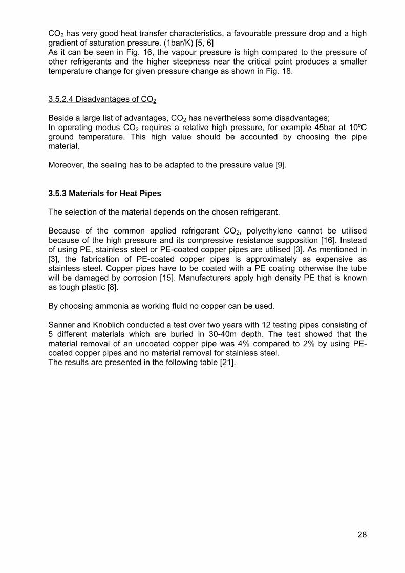
was confirmed that tubes with the smallest diameter are less sensitive to dry out. Nevertheless, in large diameter tubes dryout occurs already in shorter depth [2]. The pressure drop is the highest for the smallest pipe diameter [2]. 3.5.6 Borehole Depth The borehole varies from country to country. Generally, the borehole depth reaches from 80-350m [7]. A well-known company, M-Tech, in Austria investigates only depth up to 100m. In Sweden, however, there is a trend towards deeper drilling. In 2005 the standard depth in Germany and Austria for one family house was 60-75m [6]. In Germany the depth limit up to which no special license is required is 100m. 3.5.7 Pressure Drop for Thermosiphon Pipe The pressure drop in the borehole is caused by gravity. For small pipe diameters, friction is added but normally it is unattended [2]. Mainly in the adiabatic section friction occurs because in that section the liquid film thickness and the mass flow rate are the highest [2]. The pressure drop caused by gravity increases as the tube diameter increases. That investigation has been carried out in a model of CO2 thermosiphon that was compared to normal brine pipes [2]. For that experiment a tube diameter of 200mm for the condensing part and a variable adiabatic and evaporation part tube diameter of 12-60mm were chosen. If the pipe length exceeds a certain value the total pressure becomes supercritical and no evaporation/heat transfer takes place anymore but only a one-phase convection [15]. As declared in 3.5.2.1, the high gradient of the pressure-temperature diagram is one of the particular characteristics of CO2. A pressure drop change implies a low temperature change. Therefore, the pressure and the saturation temperature along the tube increases, which means lower heat transfer performance [6]. Fig. 21 shows the path of the pressure change. It is a geodetic profile along the tube. The temperature at the top is lower than at the bottom. The pressure changes also towards higher values at the bottom of the pipe [15].

32

Fig. 21: Pressure Profile in the Heat Pipe [15]

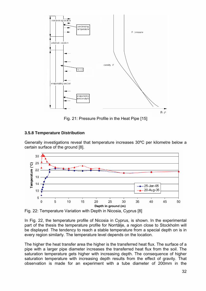
3.5.8 Temperature Distribution Generally investigations reveal that temperature increases 30ºC per kilometre below a certain surface of the ground [8].

Fig. 22: Temperature Variation with Depth in Nicosia, Cyprus [8] In Fig. 22, the temperature profile of Nicosia in Cyprus, is shown. In the experimental part of the thesis the temperature profile for Norrtälje, a region close to Stockholm will be displayed. The tendency to reach a stable temperature from a special depth on is in every region similarly. The temperature level depends on the location. The higher the heat transfer area the higher is the transferred heat flux. The surface of a pipe with a larger pipe diameter increases the transferred heat flux from the soil. The saturation temperature gets higher with increasing depth. The consequence of higher saturation temperature with increasing depth results from the effect of gravity. That observation is made for an experiment with a tube diameter of 200mm in the

33

condensing section and different tube diameters (12-60mm) for the adiabatic and evaporation part [2]. In Fig. 23 it is shown that the increase of saturation temperature of CO2 as refrigerant is about 1K/65m. It is assumed that the temperature of the ground is stable. That small temperature rise does not influence the system very much. By increasing the temperature difference the risk of destroying the liquid film trickling downwards increases. Therefore the temperature difference should be as small as possible.

Fig. 23: Simulated Temperature Increase along the Tube [6]

The more parallel pipes and evaporation area are of preference for utilising the heat and to reducing the risk of flooding according to [5]. Fig. 24 represents the temperature course in an installed test plant of the company “M-Tech” over the time. The temperature profiles relate to three depths of the 65m deep test plant. The exact depth is unknown but the curves are signified with “upper, lower and middle” part of the pipe. Fig. 24 features also the profile of the saturated CO2 temperature and of the refrigerant fluid. It should be comparable to the temperature profile curves of the experimental part with a thermosiphon loop that will be developed. One can see that the temperature of the lower part is the highest, for the upper part the pipe temperature is the lowest.

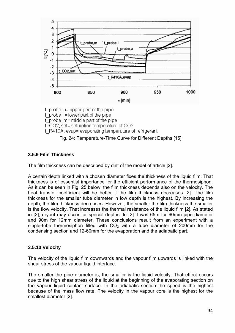
34

Fig. 24: Temperature-Time Curve for Different Depths [15]

3.5.9 Film Thickness The film thickness can be described by dint of the model of article [2]. A certain depth linked with a chosen diameter fixes the thickness of the liquid film. That thickness is of essential importance for the efficient performance of the thermosiphon. As it can be seen in Fig. 25 below, the film thickness depends also on the velocity. The heat transfer coefficient will be better if the film thickness decreases [2]. The film thickness for the smaller tube diameter in low depth is the highest. By increasing the depth, the film thickness decreases. However, the smaller the film thickness the smaller is the flow velocity. That increases the thermal resistance of the liquid film [2]. As stated in [2], dryout may occur for special depths. In [2] it was 65m for 60mm pipe diameter and 90m for 12mm diameter. These conclusions result from an experiment with a single-tube thermosiphon filled with CO2 with a tube diameter of 200mm for the condensing section and 12-60mm for the evaporation and the adiabatic part. 3.5.10 Velocity The velocity of the liquid film downwards and the vapour film upwards is linked with the shear stress of the vapour liquid interface. The smaller the pipe diameter is, the smaller is the liquid velocity. That effect occurs due to the high shear stress of the liquid at the beginning of the evaporating section on the vapour liquid contact surface. In the adiabatic section the speed is the highest because of the mass flow rate. The velocity in the vapour core is the highest for the smallest diameter [2].

35

As can be seen in Fig. 25, the velocity of the liquid at the wall is 0 and has a higher gradient near the wall. In the middle of the liquid film the profile is almost flat. The gradient of the vapour-liquid interface shows the effect of the shear stress between the vapour and the liquid. This result increases for smaller pipe diameters and may cause a flow reversal [2].

Fig. 25: Velocity Profile in the Thermosiphon Tube [11]

3.5.11 Final Design The preferred working fluid that is already used in many applications working on the thermosiphon mechanism is CO2 because of its harmlessness to the environment in combination with its excellent heat transfer values. Experiments have proven that using more than one single probe per borehole is more efficient. Nevertheless, the maximum amount of parallel installed thermosiphons is limited to 4 to ensure the sustainability [5]. 4 instead of 3 tubes in one borehole reduce the temperature drop by 14% which means 33% more heat transfer area and required material as can be seen in Fig. 27 [6]. A spiral type works quite efficient but is more difficult to fabricate and to install [5]. If the drill is inclined a minimum distance between the boreholes of 5-6m has to be kept [5]. The evaporator may be installed either on the top of the probe which leads to a split of the heat pump or the problem is solved with a little condensate return pump. In that case the COP is not much influenced but the system can no longer be advertised as self circulating system [15]. Most of the systems that have already been installed have a depth of about 80m and the pipe diameter is about 15mm.

36

On the subject of dimensioning, the VDI (association of German engineers) recommends special calculation models. (“Earth Energy Designer V2.0, published in 2000) [7]

Fig. 26: Number of Parallel Installed Thermosiphons [6]

4. DESCRIPTION OF INSTALLATION AND EXPERIMENTAL SET UP 4.1 Test Rig Setup The experimental part of the project is based on an installation in Norrtälje, a small town situated north of Stockholm. The installed test plant is organised by a Swedish company called ETM KYLTEKNIK which works in close collaboration with KTH for the thermosiphon project and which chose the material and the dimensions of the test rig. 4.1.2 Components of Test Rig The test rig mainly consists of two parts:

• Heat pump unit “Vari Scroll Optimal 6-10” produced by a company called Eureftec (www.eureftec.se). The heat pump works with R414A as refrigerant. The heat pump was self-modified and an old compressor was installed. Fig. 27 mirrors the heat pump.

37

Fig. 27: Heat Pump Test Rig

• Copper pipe unit (consisting of a straight pipe and a spiral shaped pipe) buried vertically in the ground. It will be dwelled on the design in detail in the 4.1.3. The circulating fluid inside the copper pipe is CO2.

4.1.3 Principal Design of Test Rig The test rig consists of a heat pump unit that is linked with the pipe-spiral connection. The pipe and spiral unit is inserted in a 70 m deep, vertical borehole. The spiral encloses the straight pipe and both tubes are connected at the bottom and at the top. Furthermore, the piping unit is connected with the heat pump that is installed in a small room. CO2 as fluid circulates in the buried system. Fig. 28 displays the system as an abstract drawing. On the right side of Fig. 28 the heat pump circle is displayed more detailed. The heat pump fluid passes the compressor and its pressure increases. In the condenser the fluid gives its heat to another medium carries the heat – here it warms up a room. After the condenser the fluid cools down, is expanded and in the evaporating part it takes up the heat from the passing CO2.

38

Fig. 28: Experimental Test Rig

In summary, three circuits can be distinguished:

• In the ground the CO2 circulates which gives its heat to the refrigerant cycle. • In the heat pump cycle R414A as circulating refrigerant is chosen. • The warmed R414A translates its heat to another medium for heating up a room.

The following drawing, Fig. 29, displays the test rig more abstractly. The evaporator is fed with the vapour from the spiral. The condensed liquid from the evaporator is gathered in the separator and then it is flowing downwards in the pipe. The separator is added for compounding the driving force of liquid in the loop. All these facts are based on the ideal case. Two valves are fixed to change the inlet/outlet side and to ensure the possibility to change the design of the system without emptying the whole system. In Fig. 30 the dimensions of the pipe are described explicitly. The ground water level is of vital importance. From 7m on, the heat extraction starts. Not till then the heat extraction is efficiently.

39

Fig. 29: Thermosiphon Loop First Version Fig. 30: Dimensions of the Thermosiphon As one can see in Fig. 31, the test plant of the experiment consists of a tube with 17mm inner diameter in the middle where the liquid is desired to flow downwards. At the bottom of that tube a spiral with 13mm inner diameter is fixed through which the gas should flow upwards. The spiral and the pipe are connected at the top through the heat pump evaporator. Consequently a closed loop occurs. The borehole diameter amounts to 113mm and the outer spiral diameter 100mm. One meter of pipe overlaps at the bottom of the hole, acting as extra weight and to collect any dirt from the collector inner part. Fig. 32 shows the connection between pipe and spiral in detail. The blue cover is a casing for the temperature sensors which are presented in 4.1.4. Pipe and spiral are welded together as one can see.

40

Fig. 31: Specific Dimensions of the Test Rig

Fig. 32: Arrangement of the Thermosiphon Loop

4.1.4 Measurement Instruments

• Temperature sensors: water/soil temperature sensors for HOBOH8 and U12 family data logger (TM C50-HD 50ft. = temperature sensor known value) manufactured by the company Onset. The obtained data is evaluated with the software “HOBOware pro”. The analysis of the data results in a temperature curve of the measuring points. The temperature sensors display the temperature with an accuracy of 0.25 ºC.

• Optical fibre: DTS (Distributed Temperature Sensor). A laser is sent through a fibre cable collecting a specific temperature every one meter of cable length. The saved data have to be exported into Excel and result in a graph with temperature

41

values every meter along the entire length of the fibre cable. The DTS is able to measure the temperature with an accuracy of around 0.05°C. Fig. 33 shows the design of an optical fibre utilised in DTS.

Fig. 33: Optical Fibre [DTS Manual]

It can be concluded that the optical fibre measures exacter than the temperature sensors and provides results all over the pipe not only on certain breakpoints. It is installed with an U-turn at the bottom but only the downgoing side is regarded for the analysis. Another advantage of an additional temperature measurement instrument is the assurance of reliable measurement results and functioning instruments by being able to compare the data of fibre and sensors. It is of vital importance for the further experiment that no measurement equipment was fixed on the spiral. Therefore, no information about the situation in the spiral exists. 4.1.5 The Setup and Installation Process The process of setup of the test rig took several days: on the first day the prepared copper pipes and the copper spirals pieces – each of them with a length of 7m - had to be inserted into the borehole piece by piece. Then, the following piece had to be welded. For the first connection of spiral and pipe that process already had been conducted by the supplying company. It was arranged that one meter of pipe overlaps at the bottom of the hole, constructed as collecting pond for the remainders and waste materials from the welding. After the welding, the temperature sensors were fixed one by one on the pipe and on the outer side at different points located at 15m, 35m and 70m under the ground surface. It was later decided to add an optical fibre as possibility to gather more measurement data all over the pipe and not only on three fixed points. The fibre was put between the central pipe and the spiral. It was not fixed on the pipe. Therefore, the exact location is unknown. Another subsequent decided modification was the insulation of the inner pipe. The chosen insulation material was Tubolit DG-A 22/13 with a conductivity of k=0.035 W/mK. The insulation should prevent the downgoing liquid to evaporate before it reaches the bottom. Since it was a late decision, the insulation reached the first upper 42m.

42

For the upper 42m the optical fibre is located outside the insulation. For the lower part it is located somewhere between the pipe and the borehole. Subsequently, the piping circuit and the heat pump were connected. Two valves, one on the central pipe and one on the spiral side were fixed to change flexibly the inlet/outlet feeding pipe for the CO2. A manometer was fixed on the highest point of the system and also a sensor that measures the CO2 concentration was added. In case of leakage that might give information about the rise in CO2 concentration. Moreover, a relief valve that opens if 60bar are exceeded was fixed. All pipes and the separator were insulated. Before filling the closed loop with CO2, it was evacuated with a vacuum pump. It was decided to fill liquid CO2 into the spiral. The company ETM Kylteknik checked that no leakage of CO2 occurred. The first filling amount that was weighed was 9kg of CO2 (liquid phase). The amount of CO2 that was added was then increased because no circulation of the fluid could be noticed at the project’s early stage. Finally, the amount reached 14,4kg. At this value the filling stopped for the first time. For this measurement period the optical fibre was not yet in operation. During the measurements the amount of CO2 was varied several times. 4.2 Previous Calculations Before starting the measurements some calculations and analysis should be carried out regarding the pressure drop and the filling rate in the thermosiphon loop. 4.2.1 Pressure Drop For the calculations of the pressure drop in the tube and the spiral some assumptions are inevitable. It is assumed that the ideal case, that means an appearance of phase change at the bottom and on the top of the linked pipes, occurs. Liquid should flow downwards in the pipe and vapour likewise upwards in the spiral. For the calculation it is simplified that the spiral is considered as a straight pipe with its total length. The calculated values for the pressure drop in both pipes have to be compared in order to determine the flow direction of the loop. The pressure drop of the liquid system is assumed to be caused mainly by gravity, acceleration and friction:

liquidonacceleratiliquidfrictionliquidgravityliquid pppp ,,, Δ+Δ+Δ=Δ (1) The vapour system acts equally:

vapouronaccelerativapourfrictionvapourgravityvapour pppp ,,, Δ+Δ+Δ=Δ (2) The particular equations are as follows:

43

hgp gasCOvapourgravity ⋅⋅=Δ ,, 2ρ (3) (equivalent for liquid phase)

dLwfp gasCOvapourfriction ⋅⋅⋅=Δ 2

,, 2ρ (4) (equivalent for liquid phase)

υ⋅=Δ 2

, Gp vapouronaccelerati (5) (equivalent for liquid phase) For the calculation of the pressure drop caused by friction it is moreover necessary to determine the Reynolds Number:

ηρ

ν⋅⋅

=⋅

=DwDwRe (6)

If Re > 2300: turbulent flow If Re < 2300: laminar flow For the laminar flow the following simplification of the equation (4) is necessary:

Re64

=f (6)

For the turbulent flow it is:

4/1Re3164,0

=f (7)

Due to the fact that the velocity is needed in equation (6) the following simplifications are applied:

The equation of continuity is: (with 2

4dA Π

= )

ρ⋅⋅= Awm& (8) The mass flux can be calculated by dint of equation 9 and can be simplified by using equation 8.

wAmG ⋅== ρ&

(9)

Furthermore the mass flow can be expressed as:

hxQm⋅

=&

& and ''' hhh −= (10)

With h=h’-h’’ as enthalpy difference between liquid and vapour enthalpy. Q& indicates the heat flow that is fixed from the following assumption: as investigated in [27] the heat

44

extraction rate in Sweden is about 40W/m. (see 1.6) The borehole length of the test rig is 70m which leads to Q& = 2800 J/s or 2800W. Density and enthalpy values are taken from the attached table of chemical data of CO2. (Appendix A) The calculated pressure drop in the pipe should be higher than the pressure drop in the spiral so that the system is forced to circulate in the desired direction. The sum of the pressure drop in the pipe compared to the pressure drop in the spiral resulted to be: ∆ppipe = 606302,501Pa = 6,063bar ∆pspiral = 101191,977Pa = 1,012bar Therefore, it seems to circulate in the desired manner according to the assumptions that were made above. The complete results of the calculations are attached as appendix B. See appendix B: 1. Calculations of Pressure Drop (gravity)

2. Calculations of Pressure Drop (friction) 3. Calculations of Pressure Drop (acceleration)

4.2.2 Filling Rate Another fact that has to be defined in advance is the amount of CO2 that should be added to the system. The published papers [22, 26] agree on a filling rate of 70%-80% for a double-tube thermosiphon loop. The researchers assert that for that amount the heat transfer rate proves to be the best. For the amount of the CO2 mass in the ideal filling case of 80%, the total volume of the system should be calculated and multiplied with the density. All required values refer to a temperature of 7ºC and the values refer to

the liquid phase. (The necessary equations are hdV ⋅Π

= 2

4 and Vm ⋅= ρ )

The result was 27 kg CO2 (liquid gaseous state). This theoretical value will be compared with the experimental value. Unfortunately the filling amount was an uncertain factor during the measurements, therefore the comparison between the theoretical and experimental value could not be conducted. Appendix C includes the filling rate calculation results. 4.3 Planned Measurements The attached temperature sensors are fixed on the pipe to measure the temperature of the CO2. The conductivity of copper is 397W/mK [23]. Hence, it can be stated that the thickness of the copper pipe does not influence the measurement result. The other three sensors are put on the borehole side, whose temperature refers to the groundwater temperature. The location of the sensors is additionally shown in Fig. 35.

45

Fig. 34: Location of Temperature Sensors

In Fig. 35 it is observed that the temperature measurement points are located at 15m, 40m and 70m. One sensor is fixed inside the insulation and outside the insulation. 4.4 Testing Method Before dwelling on the exact testing method, the variable parameters of the test rig have to be defined. The measurement equipment gives out temperature data. The temperature is given by the ambient ground temperature. That implies no possibility to influence that parameter. The pressure is measured on the top of the pipe where the vapour is stored in the steady state. For the vapour, the pressure is equal in the closed system and the height difference is disregarded. The pressure can only be changed in a closed system with one-phase. However, since the thermosiphon is a two-phase system, the pressure is predetermined by the temperature. The only parameter that can be varied is the filling rate of CO2. Therefore, the testing method contains the change of the CO2 filling rate. In spite of the calculated data, it was decided to increase the filling from a low level step by step to a high level. After the borehole heat exchanger is filled with CO2, the experiment is carried out in the following way:

1. Measurements of the undisturbed ground 2. Start the system 3. Collecting temperature data while the heat pump is running

46

4. Checking the CO2 concentration level and the pressure of the manometer while the heat pump is running

5. Analysing the data for the running system first design 6. Analysing the data for the running system modified system 7. Comparison 8. Discussion of results

4.5 Occurrence of Difficulties during the Installation Process One problem appeared even during the first installation day. The first meters of the pipe were lifted because it was trapped in the ground and the borehole heat exchanger bended while taking it up. The result of the bending could have a permanent negative impact on the shape of spiral and pipe since the change in cross section might change the flow conditions in the collector. 4.6 Modification of Design At a secondary development stage of the project the system was modified. Henceforth, the separator has two outgoing pipes and one incoming pipe. The incoming pipe transports the condensed liquid from the evaporator. The outgoing pipe at the bottom of the accumulator feeds the collector’s central pipe with liquid. The outgoing pipe at the top is for the vapour that may be generated in the pipe to go back to the evaporator. Fig. 35 displays a schematic sketch of the modified design.

Fig. 35: Modified Design of Thermosiphon Loop

47

5. DISCUSSION OF RESULTS 5.1 Undisturbed Ground 5.1.1 Temperature Sensors The temperature of the undisturbed ground can be verified with the measurement results of the temperature sensors. Therefore, an interval of 12 hours was chosen between the 5th February and the 6th February 2008. During that period the system was untouched. The sensors recorded data every 2 minutes. The measurement started at 19:51:38 and ended at 07:59:09. (Central European Time - CET)

Fig. 36: Undisturbed Ground, Temperature Sensors on the Pipe (5th-6th Feb.2008)

Fig. 37: Undisturbed Ground, Temperature Sensors on the Borehole (5th-6th Feb.2008)

48

Fig. 36 mirrors the temperature distribution given by the temperature sensors connected on the pipe (i.e. between the insulation and the copper pipe) at 15m, 40m and 70m. It is obvious that the temperatures are stable over the time period. The highest temperature was recorded at 15m of depth with a value of about 7,8 °C and the lowest was approximately 6,5 °C at 40m. Fig. 37 gives more exact values of the undisturbed ground temperature over the borehole length. The temperature values taken with sensors on the borehole side (outside the insulation) show certain deviation with respect with the ones shown in Fig. 36 at 40 meters depth. For 15 and 70 meters, Fig. 37 shows the same tendency. The variation of the 40m data will be verified by dint of the optical fibre. The calculated maximal difference between pipe and borehole temperature at 15 meters was 0,08ºC. In 70m depth the maximal difference was 0,10ºC. A third graph (Fig. 38) is shown. It compares the temperatures on the pipe and on the borehole side for 15, 40 and 70m. In 40m depth a high difference can be observed. It seems that one sensor is damaged. Later the optical fibre verifies that supposition.

Fig. 38: Undisturbed Ground, Temperature Sensors, Comparison (5th-6th Feb.2008)

5.1.2 Optical Fibre

Fig. 39 shows the temperature distribution of the undisturbed ground in Norrtälje overnight from the 5th to 6th February 2008. During that period the ground was absolutely undisturbed. The optical fibre measured every half an hour making average for 10 minutes periods during the measurement time. It made an average of all values that are measured in ten minutes. An average temperature of every meter of cable length was taken during the measured period. For the analysis, the down going optical fibre was chosen because that gives more accurate data.

49

Fig. 39: Undisturbed Ground, Optical Fibre (5th-6th Feb.2008)

The exact profile of the temperature in the borehole is shown in Fig. 39 confirming the results of the temperature sensors. The highest temperature happens between 5-15m and the lowest temperature occurs from 35-45m. From there the temperature increases again. The starting point was 0 meters of depth, which means the ground surface. For that point the temperature was about 9,5ºC. That high value occurred because the test rig is installed inside a room. At 7m (the ground water level) the real heat extraction starts. (“Active borehole depth”) Fig. 40 shows the temperature distribution in 15, 40 and 70m depth to improve the possibility to compare the optical fibre measurements with those of the temperature sensors. Start: 20:54h Stop: 08:54h (CET)

Fig. 40: Undisturbed Ground, Optical Fibre, Different Depth (5th-6th Feb.2008)

The calculated highest temperature difference for 15m was 0,11ºC and for 70m 0,24ºC. It can be stated that the fluctuations at 70m are higher than at 15m. A reason for the

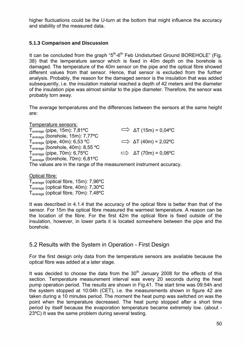
50

higher fluctuations could be the U-turn at the bottom that might influence the accuracy and stability of the measured data. 5.1.3 Comparison and Discussion It can be concluded from the graph “5th-6th Feb Undisturbed Ground BOREHOLE” (Fig. 38) that the temperature sensor which is fixed in 40m depth on the borehole is damaged. The temperature of the 40m sensor on the pipe and the optical fibre showed different values from that sensor. Hence, that sensor is excluded from the further analysis. Probably, the reason for the damaged sensor is the insulation that was added subsequently, i.e. the insulation material reached a depth of 42 meters and the diameter of the insulation pipe was almost similar to the pipe diameter. Therefore, the sensor was probably torn away. The average temperatures and the differences between the sensors at the same height are: Temperature sensors: Taverage (pipe, 15m): 7,81ºC ∆T (15m) = 0,04ºC Taverage (borehole, 15m): 7,77ºC Taverage (pipe, 40m): 6,53 ºC ∆T (40m) = 2,02ºC Taverage (borehole, 40m): 8,55 ºC Taverage (pipe, 70m): 6,75ºC ∆T (70m) = 0,06ºC Taverage (borehole, 70m): 6,81ºC The values are in the range of the measurement instrument accuracy. Optical fibre: Taverage (optical fibre, 15m): 7,96ºC Taverage (optical fibre, 40m): 7,30ºC Taverage (optical fibre, 70m): 7,48ºC It was described in 4.1.4 that the accuracy of the optical fibre is better than that of the sensor. For 15m the optical fibre measured the warmest temperature. A reason can be the location of the fibre. For the first 42m the optical fibre is fixed outside of the insulation, however, in lower parts it is located somewhere between the pipe and the borehole. 5.2 Results with the System in Operation - First Design For the first design only data from the temperature sensors are available because the optical fibre was added at a later stage. It was decided to choose the data from the 30th January 2008 for the effects of this section. Temperature measurement interval was every 20 seconds during the heat pump operation period. The results are shown in Fig.41. The start time was 09:54h and the system stopped at 10:04h (CET), i.e. the measurements shown in figure 42 are taken during a 10 minutes period. The moment the heat pump was switched on was the point when the temperature decreased. The heat pump stopped after a short time period by itself because the evaporation temperature became extremely low. (about -23ºC) It was the same problem during several testing.

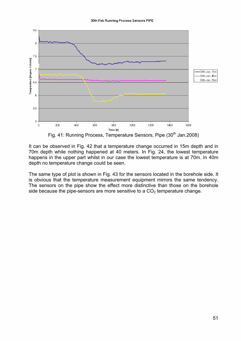
51

Fig. 41: Running Process, Temperature Sensors, Pipe (30th Jan.2008)

It can be observed in Fig. 42 that a temperature change occurred in 15m depth and in 70m depth while nothing happened at 40 meters. In Fig. 24, the lowest temperature happens in the upper part whilst in our case the lowest temperature is at 70m. In 40m depth no temperature change could be seen. The same type of plot is shown in Fig. 43 for the sensors located in the borehole side. It is obvious that the temperature measurement equipment mirrors the same tendency. The sensors on the pipe show the effect more distinctive than those on the borehole side because the pipe-sensors are more sensitive to a CO2 temperature change.

52

Fig. 42: Running Process, Temperature Sensors, Borehole (30th Jan.2008)

The 40m line from Fig. 42 should not be regarded since it shows the data of the damaged sensor. 5.3 Results with the System in Operation – Modified Test Rig This section refers to the modified test rig as shown in Fig. 36. The data are picked out from the 7th February 2008. This section it is more focused on the optical fibre data because it represents the temperature all over the borehole. For the modified design the optical fibre was installed additionally. 5.3.1 Temperature Sensors The chosen interval for measurement with the sensors was every 20 seconds. Fig. 45 shows a set of data taken with start at 09:05h and end at 09:17h (CET) for the points located between the pipe and the insulation. In 15m depth a temperature change can be observed. The temperature in 15m and 40m depth is almost stable. In 40m depth the temperature decreases 0,4ºC over the running period. Those occurrences seem to be the main difference between first and modified design.

53

Fig. 43: Modified Running Process, Temperature Sensors, Pipe (7th Feb.2008)

Fig. 44: Modified Running Process, Temperature Sensors, Borehole (7th Feb.2008)

For the borehole-sensors the course is similar. The curve for 40m is not shown because of the irregularities of the sensor. The change of temperature only occurs in 15m depth. The 70m temperature distribution is almost stable – equal to the pipe-sensor results.

54

Furthermore, Fig. 45 shows how the system stabilised after the heat pump running process ended. This is accomplished by dint of measured data with the sensors which were recorded on the 7th Feb 2008. It takes 350s to increase the temperature 0,5ºC which was unexpected.

Fig. 45: Stabilisation of the System, Temperature Sensors (7th Feb.2008) 5.3.2 Optical Fibre During the heat pump running process, the interval for gathering measurements with the optical fibre was reduced to every 20s. Fig 46 presents the measurements between 09:08h and 09:20h (CET).

55

Fig. 46: Modified Running Process, Optical Fibre (7th Feb.2008)

The tendency of the optical fibre is similar to the pipe and borehole measurements. In 15m depth a temperature change can be noticed. The fluctuations are higher and the curves even cross each other. The optical fibre is more sensitive to ambient effects than the sensors as explained above. During the running period it seems that the data are influenced considerably by the moving CO2. In addition, a plot of the temperature course during a running process compared to the undisturbed ground is shown in Fig. 47 for the same period.

Fig. 47: Comparison Modified Running Process and Undisturbed Ground, Optical Fibre

(7th Feb. 2008)

56

The purple-triangle-line mirrors the highest temperature, representing the undisturbed ground. The other curves show the course of the temperature during the running process 7, 11 and 13 minutes after the heat pump starts. It can be stated that the temperature decreases continually between 15m and 40m for that special filling rate. The other temperatures in the borehole are almost constant and independent of the heat pump operation time. Moreover, it was detected that the temperature interval is lower if several running times are done in succession. Figure 48 and 49 show how the temperature course changes. Fig. 48 shows data for the modified system on February 14th, 2008 for the moment when the heat pump starts, stops and in the middle of the running interval. Start time 1: 08:06h Stop time 1: 08:16h Fig. 49 represents the second running interval. Start time 2: 09:23h Stop time 2: 09:27h (CET) The first running process took 10 minutes, the second 4 minutes.

Fig. 48: Modified Running Process, Optical Fibre (7th Feb. 2008 (1))

57

Fig. 49: Modified Running Process, Optical Fibre (14th Feb. 2008 (2))

Fig. 48 shows a temperature change in the borehole when the heat pump starts. However, in Fig. 49 the heat pump stopped by itself after 4minutes and no movement of temperature can be stated. The same behaviour could be noticed with the temperature sensors. That effect occurred every time of subsequently measurements. The temperature of the system is too low to force the CO2 to circulate. 5.3.3 Comparison and Discussion With the modified design, both measurement instruments present a temperature change only at 15m depth. The trend is the same for all conducted measurements. That leads to the assumption that the modified test rig design changed the point of evaporation of the CO2 in the borehole heat exchanger. It is suspected that, in the modified design, the vapour could flow upwards. The filling amount of the CO2 is unknown but there is certainly a liquid column. This is certain because the pressure was not changeable. This indicates a two-phase system. It seems that the liquid evaporates on its way downwards, inverts its direction and flows directly upwards as vapour.

6. CONCLUSIONS The CO2 did not circulate. It seems that the calculated pressure drop cannot be verified by the experiment. Probably, the assumptions and the calculations were not specific enough. One reason for the lack of circulation could be that the dimensions of the system were chosen incorrect. The modified version of the system did not show any amelioration. The only thing that changed was the level / point of evaporation. The results of the 40m borehole sensor were not reliable. The tendency was all the same – the 40m borehole sensor seems to be damaged.

58

The measurement interval always was 10-15minutes when the heat pump was in operation, if the system was able to stabilise some hours. If some tests were made successively, the time interval decreased as it was shown in 5.3.2.

7. PROBLEMS AND RECOMMENDATIONS One problem was the high CO2 concentration in the room. The normal value of concentration is about 300ppm. After the testing period the value changed to 1790ppm. That value is extremely high and exceeds the required CO2 concentration limit in a closed room. That occurrence caused extensive discussions about the existence of a leakage. It is supposed that at least no leak in the ground exists but that the valves and the connection piece between piping unit and the CO2 bottle are not completely leak prove. It was remarkable that the pressure manometer showed no change. If the loop is leaky the pressure should decrease within some days. What can be reasoned definitely is that CO2 leaks from a source. Due to several changes of the test rig design the value of filling rate got lost. One temperature sensor showed nonsensical results. Probably it was damaged during the installation process. The heat pump also has encountered difficulties. The expansion valve was contaminated and had to be cleaned to retrieve its functionality. In addition, the compressor broke down but it could be repaired. Moreover, the time interval of the running process was extremely short. After 5-10 minutes the heat pump switched off by itself. Different modifications were made to see if the running interval extends or not but we did not succeed to extend the running interval into a longer working period. The pressure drop calculations have to be modified. Nevertheless, it is supposable that the spiral diameter was chosen too small. The factor of friction in the spiral is higher than in the pipe, anyhow, the spiral diameter is even lower than that of the pipe. Therefore, the dimensions of the test rig have to be reconsidered. The diameter of the spiral has to be bigger than that of the pipe. An additional pressure measurement instrument would be appreciated for further research. In addition, a further project can deal with the pressure calculation in a thermosiphon loop for domestic applications. Obviously, more information and research are necessary to improve the design and or to propose new design suggestions. The project will go on and the following student can continue with the analysis of the modified design. If that proposal is not working the system will be filled up with a glycol-water mixture and will work like it is explained in 1.6.2. The final improvement is to order a circulating pump. This pump should push on the fluid inside that it gets circulating. It can either be used permanently or just to give an impulse to the system that it gains momentum. The producer of the chosen pump is called “Hysave”. Further information can be found on the web page www.hysave.at.

59

The original separator is replaced by a bigger one which can accumulate even more liquid to increase the driving force. Moreover, sight glasses are fixed so that the liquid level in the separator can be controlled.

8. SUMMARY AND OUTLOOK Regrettably the circulation of CO2 is missing. It cannot be defined exactly due to which reasons but some possibilities are offered in chapter 7. It was difficult to interpret the graphs without knowledge how the curve should look like for a thermosiphon loop. The only clue is the graph presented in Fig. 24. However, that is the profile for a one-tube thermosiphon. For understanding the absence of circulation it is essential to have additional measurement points on the spiral. With the achieved results nothing can be stated about the situation in the pipe. Moreover, the pressure course is of great interest. As could be seen from the calculations the spiral was considered as straight pipe and some other simplifications were made. There are much more factors that have to be taken into account such as the incline of the borehole, the welding crossing and the resulting change of cross section, the gradient of the spiral shape and so on. However, the potential of the thermosiphon loop is huge and the test rig offers possibilities to gather more information about that topic.

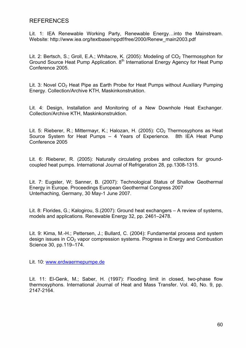
60

REFERENCES Lit. 1: IEA Renewable Working Party, Renewable Energy…into the Mainstream. Website: http://www.iea.org/textbase/nppdf/free/2000/Renew_main2003.pdf Lit. 2: Bertsch, S.; Groll, E.A.; Whitacre, K. (2005): Modeling of CO2 Thermosyphon for Ground Source Heat Pump Application. 8th International Energy Agency for Heat Pump Conference 2005. Lit. 3: Novel CO2 Heat Pipe as Earth Probe for Heat Pumps without Auxiliary Pumping Energy. Collection/Archive KTH, Maskinkonstruktion. Lit. 4: Design, Installation and Monitoring of a New Downhole Heat Exchanger. Collection/Archive KTH, Maskinkonstruktion. Lit. 5: Rieberer, R.; Mittermayr, K.; Halozan, H. (2005): CO2 Thermosyphons as Heat Source System for Heat Pumps – 4 Years of Experience. 8th IEA Heat Pump Conference 2005 Lit. 6: Rieberer, R. (2005): Naturally circulating probes and collectors for ground-coupled heat pumps. International Journal of Refrigeration 28, pp.1308-1315. Lit. 7: Eugster, W; Sanner, B. (2007): Technological Status of Shallow Geothermal Energy in Europe. Proceedings European Geothermal Congress 2007 Unterhaching, Germany, 30 May-1 June 2007. Lit. 8: Florides, G.; Kalogirou, S.(2007): Ground heat exchangers – A review of systems, models and applications. Renewable Energy 32, pp. 2461–2478. Lit. 9: Kima, M.-H.; Pettersen, J.; Bullard, C. (2004): Fundamental process and system design issues in CO2 vapor compression systems. Progress in Energy and Combustion Science 30, pp.119–174. Lit. 10: www.erdwaermepumpe.de Lit. 11: El-Genk, M.; Saber, H. (1997): Flooding limit in closed, two-phase flow thermosyphons. International Journal of Heat and Mass Transfer. Vol. 40, No. 9, pp. 2147-2164.

61

Lit. 12: European Renewable Energy Council (EREC) (2007): RENEWABLE HEATING – ACTION PLAN FOR EUROPE. Website: http://www.erec.org/documents/publications.html Lit. 13: Heat Sources – Technology, Economy and Environment. Collection/Archive KTH, Maskinkonstruktion. Lit. 14: Revival of Carbon Dioxide as a Refrigerant. Collection/Archive KTH, Maskinkonstruktion. Lit. 15: Bassetti, S.; Rohner, E.; Peterlunger, A.; Ehrbar, M. (2007): Pumpenlose Erdwärmesonde Schlussbericht. Im Auftrag des Bundesamtes fuer Energie. Lit. 16: Mittermayr. K.: Information Material from K. Mittermayr, M-Tech, Austria Lit. 17: Hubert, H.: Die CO2 Sonde zur Nutzung der Erdwärme mit Wärmepumpenanlagen. Arsenal Research, Erneuerbare Energie. Lit. 18: Bassetti, S.; Rohner, E.; Signorelli, S.; Matthey, B. (2006): Dokumentation von Schadensfällen bei Erdwärmesonden. Schlussbericht Energie Schweiz. Lit. 19: Unk, J. (1989): Betriebsfuellhöhe eines geschlossenen Zweiphasenthermosiphons. KI – Klima-Kälte-Heizung 7-8. Lit. 20: Hellström, G. (2006): Market and Technology in Sweden. Lund University. Website: www.geothermie.de/groundhit/ghw/WS%2006%2012aHellstroem.pdf Lit. 21: Kruse, H.; Ruessmann, H.; Stadtländer, C. (2004): Entwicklung einer CO2-Erdwärmesonde nach dem Prinzip des Wärmerohres. KI-Kälte-Klima-Heizung 2, pp. 54-61. Lit. 22: Rafferty, K. (2000): DESIGN ISSUES IN THE COMMERCIAL APPLICATION OF GSHP SYSTEMS IN THE U.S. GHC Bulletin. Lit. 23: Ruge, J.; Wohlfahrt, H. (2007): Technologie der Werkstoffe. Vieweg Verlag, 8th Edition, pp. 140. Lit. 24: Le Feuvre, P. (2007): An Investigation into Ground Source Heat. MSc.Thesis, University of Strathclyde.

62

Lit. 25: Lit. 8: Thermal Characteristics of a Thermosyphon Heated Enclosure. Collection/Archive KTH, Maskinkonstruktion. Lit. 26: Fukuda, K.; Nakagawa, K.; Okabe, K. (1991): Thermal Characteristics of Double-Tube Two-Phase Thermosiphon. Trans. JSME, 57 (534), 687-692. Lit. 27: Andy Pearson (2005): Carbon dioxide—new uses for an old refrigerant. International Journal of Refrigeration 28, pp. 1140–1148. Lit. 28: Domestic Installation of Microgeneration Equipment; Heat Pumps. Website: www.communities.gov.uk/documents/planningandbuilding/pdf/320521.pdf

63

Appendix A: Table of Chemical Data of CO2 [Based on NIST Refprop]

Appendix B: Calculations of Pressure Drop 1.

64

2.

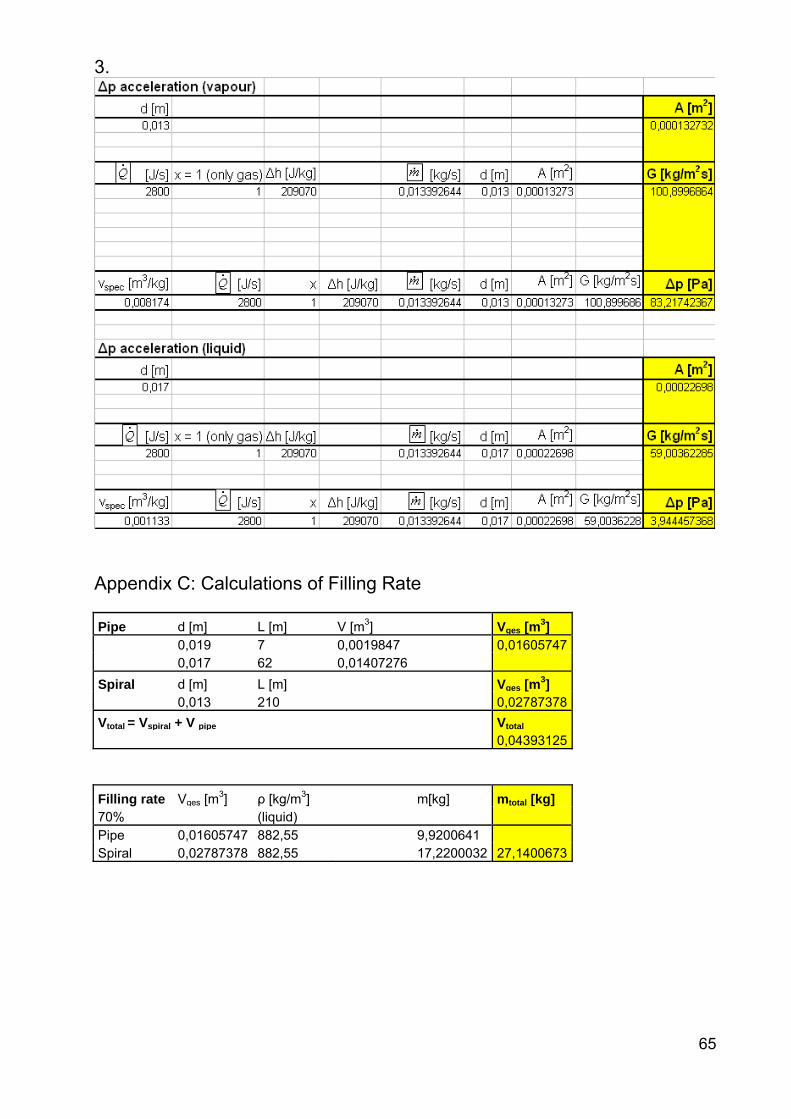
65

3.

Appendix C: Calculations of Filling Rate Pipe d [m] L [m] V [m3] Vges [m3] 0,019 7 0,0019847 0,01605747 0,017 62 0,01407276 Spiral d [m] L [m] Vges [m3] 0,013 210 0,02787378 Vtotal = Vspiral + V pipe Vtotal 0,04393125

Filling rate Vges [m3] ρ [kg/m3] m[kg] mtotal [kg] 70% (liquid) Pipe 0,01605747 882,55 9,9200641 Spiral 0,02787378 882,55 17,2200032 27,1400673