Thermodynamic Performance Evaluation and Experimental Study of a Marnoch Heat Engine
114
Thermodynamic Performance Evaluation and Experimental Study of a Marnoch Heat Engine By Pooya Saneipoor A Thesis Submitted in Partial Fulfillment of the Requirements for the Degree of Master of Applied Science in Mechanical Engineering Faculty of Engineering and Applied Science University of Ontario Institute of Technology October 2009 © Pooya Saneipoor, 2009
Transcript of Thermodynamic Performance Evaluation and Experimental Study of a Marnoch Heat Engine

Thermodynamic Performance Evaluation and
Experimental Study of a Marnoch Heat Engine
By
Pooya Saneipoor
A Thesis Submitted in Partial Fulfillment
of the Requirements for the Degree of
Master of Applied Science in Mechanical Engineering
Faculty of Engineering and Applied Science
University of Ontario Institute of Technology
October 2009
© Pooya Saneipoor, 2009
i
Abstract
The Marnoch Heat Engine (MHE) is a recently patented type of new heat engine that
produces electricity from lower temperature heat sources. The MHE utilizes lower
temperature differences to generate electricity than any currently available
conventional technologies. Heat can be recovered from a variety of sources to
generate electricity, i.e., waste heat from thermal power plants, geothermal, or solar
energy. This thesis examines the performance of an MHE demonstration unit, which
uses air and a pneumatic piston assembly to convert mechanical flow work from
pressure differences to electricity. This thesis finds that heat exchangers and the
piston assembly do not need to be co-located, which allows benefits of positioning the
heat exchangers in various configurations. This thesis presents a laboratory-scale,
proof-of-concept device, which has been built and tested at the University of Ontario
Institute of Technology, Canada. It also presents a thermodynamic analysis of the
current system. Based on the MHE results, component modifications are made to
improve the thermal performance and efficiency. The current configuration has an
efficiency of about thirty percent of the maximum efficiency of a Carnot heat engine
operating in the temperature range of 0oC to 100oC. The analysis and experimental
studies allow future scale-up of the MHE into a pre-commercial facility for larger
scale production of electricity from waste heat.
Key Words
Marnoch Heat Engine; Heat Recovery; Energy; Exergy; Efficiency, Power Cycle;
Carnot Cycle.

ii
Dedication
This research is dedicated to Ian Marnoch.

iii
Acknowledgments
I am highly indebted to several people for their extended help given to me during the
work of this entire thesis. This would not have been possible without them. It is a
pleasure to thank those who made this possible and I would like to express my sincere
gratitude and appreciation to my co-advisors: Professor Greg Naterer and Professor
Ibrahim Dincer for providing me the unique opportunity to work in this research area
under their expert guidance. I owe my deepest gratitude to Mr. Ian Marnoch who has
helped me all the way. He made available his support in a number of ways. The most
valuable source was his wealth of knowledge that helped me in completing this thesis.
Also, support of this research from Marnoch Thermal Power, the Ontario
Centres of Excellence and OPA is gratefully appreciated.
I am also indebted to many of my colleagues: O. Jaber, P. Bahadorani, S.
Garmisiry, P. Regulagada, H. Nojoumi, R. Rashidi, V. Balah, and A. Odukoya who
have helped me in terms of guidance and moral support.
In the end, I would like to express my honest and eternal gratitude towards my
parents: Darab and Masoudeh, to my siblings: Parya, Peyman, and also to Hamid and
Shervin who have been really influential. They have shown everlasting and
unconditional love, support and encouragement. Thank you for your concerns, which
gave me a chance to prove and improve myself through all phases of my life.
iv
Table of Contents
Abstract ........................................................................................................................... i
Acknowledgments........................................................................................................ iii
List of Tables ............................................................................................................. viii
List of Figures ............................................................................................................... ix
Nomenclature ............................................................................................................... xii
Chapter 1: Introduction .................................................................................................. 1
1.1 Energy and Its Importance .......................................................................................1
1.2 Motivation and Objectives .......................................................................................6
Chapter 2: Literature Review ......................................................................................... 7
2.1 Background .............................................................................................................. 8
2.2 Gas Power Cycles .................................................................................................... 9
2.2.1 The Carnot Cycle ................................................................................................ 10
2.2.2 Stirling Cycle ...................................................................................................... 12
2.3 Stirling Engines ...................................................................................................... 12
2.4 Different Configurations of Stirling Engines ......................................................... 14
2.4.1 Alpha Configuration of the Stirling Engine ........................................................ 14
2.4.2 Beta Configuration of the Stirling Engine .......................................................... 15
2.4.3 Gamma Configurations of the Stirling Engine ................................................... 16
2.4.4 Low-temperature Differential Heat Engines ....................................................... 17

v
Chapter 3: The Marnoch Heat Engine ......................................................................... 18
3.1 Energy Conversion Steps and Processes................................................................ 18
3.2 System Operation ................................................................................................... 19
3.3 Description of MHE ............................................................................................... 21
3.4 Comparison of Marnoch and Stirling Engines....................................................... 23
3.5 Materials of Construction for MHEs ..................................................................... 24
3.6 Heat Exchanger Specifications .............................................................................. 25
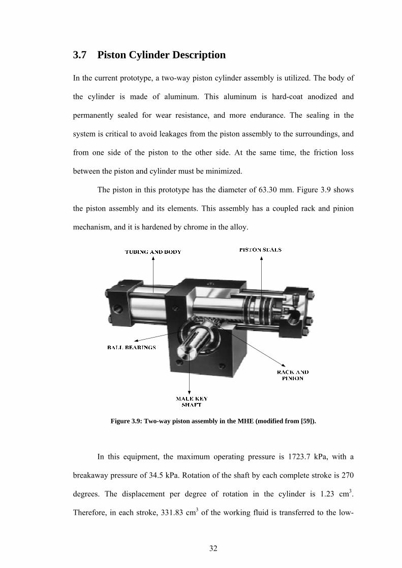
3.7 Piston Cylinder Description ................................................................................... 32
3.8 Control Valves ....................................................................................................... 35
Chapter 4: Performance Analysis ................................................................................ 38
4.1 Thermodynamic Analysis ...................................................................................... 38
4.1.1 Mass Balance of Tank 1 ...................................................................................... 41
4.1.2 Energy Analysis of Tank 1 ................................................................................. 43
4.1.3 Exergy Analysis of Tank 1 ................................................................................. 46
4.1.4 Mass Balance of the Piston Assembly ................................................................ 48
4.1.5 Energy Analysis of the Piston Assembly ............................................................ 49
4.1.6 Exergy Analysis of the Piston Assembly ............................................................ 50
4.1.7 Calculation of Shaft Work Output of the Piston Assembly ................................ 51
4.1.8 Mass Balance of Tank 2 ...................................................................................... 54
4.1.9 Energy Analysis of Tank 2 ................................................................................. 55
4.1.1 Exergy Analysis of Tank 2 ................................................................................. 57

vi
4.2 Transmission System ............................................................................................. 57
4.3 Efficiencies ............................................................................................................ 59
4.3.1 Thermal (Energy) Efficiency of the Cycle .......................................................... 59
4.3.2 Overall Efficiency of the Engine ........................................................................ 60
4.3.3 Carnot Efficiency ................................................................................................ 60
4.3.4 Exergy Efficiency ............................................................................................... 61
4.4 Uncertainty Analysis .............................................................................................. 62
Chapter 5: Results and Discussion ............................................................................... 64
5.1 Effects of Increasing the Pre-charge Pressure inside the Tanks ............................ 64
5.2 Mechanical Efficiency of Transmission System.................................................... 67
5.3 Efficiency of Mechanical Components in the MHE .............................................. 68
5.4 Pressure Measurements of MHE ........................................................................... 68
5.5 Power Output Measurements from MHE .............................................................. 70
5.6 System Efficiency .................................................................................................. 74
5.7.1 Possible Improvements of the Current System ................................................... 80
5.7.2 Possible Designs for the Next Marnoch Heat Engine Prototype ........................ 81
5.7.2.1 Application of Multiple Tank Pairs ................................................................. 82
5.7.2.1.1 MHE with Multiple Pairs of Tanks and One Electric Generator .................. 83
5.7.2.1.2 MHE with Separated Generators .................................................................. 85
5.7.3 Marnoch Heat Engine with Hydraulic Motors .................................................... 86
Chapter 6: Conclusions and Recommendations for Future Research .......................... 92

vii
6.1 Conclusions ............................................................................................................ 92
6.2 Recommendations for Future Research ................................................................. 92
References .................................................................................................................... 94

viii
List of Tables
Table 2.1: Comparison of processes for different gas power-cycles ........................... 11
Source: [38, 40] ............................................................................................................ 11
Table 3.1: Shell side of seat exchanger specifications ................................................. 29
Table 3.2: Helical coil specifications ........................................................................... 31
Table 3.3: Straight pass tubes specifications ............................................................... 31
Table 3.4: Torque output of the piston ......................................................................... 33
Table 5.1: Transmission and generator efficiency ....................................................... 67

ix
List of Figures
Figure 1.1: Distribution of energy from 1990 to 2095 (from [10]). ............................. 3
Figure 1.2: World electricity generation by source of energy (from [13]). ................... 3
Figure 2.1: Four main thermodynamic processes in power-cycles.............................. 10
Figure 2.2: Carnot cycle (a) P-V diagram; (b) T-s diagram. ....................................... 11
Figure 2.3: Stirling cycle (a) P-V diagram; (b) T-s diagram. ...................................... 12
Figure 2.4: Schematic of the Alpha configuration of the Stirling engine (modified
from [46]). .................................................................................................................... 15
Figure 2.5: Schematic of the Beta configuration of a Stirling heat engine (modified
from [49]). .................................................................................................................... 15
Figure 2.6: Schematic of the Gamma Configuration of the Stirling engine (modified
from [49]). .................................................................................................................... 16
Figure 3.1: The working stages of energy conversion in a Marnoch heat engine. ...... 18
Figure 3.2: Schematic of the MHE configuration with two pairs of tanks (modified
from [57]). .................................................................................................................... 20
Figure 3.3: Photos of the (a) current prototype and (b) transmission. ......................... 21
Figure 3.4: Connection diagram of the current prototype of the MHE with two pairs of
tanks. ............................................................................................................................ 23
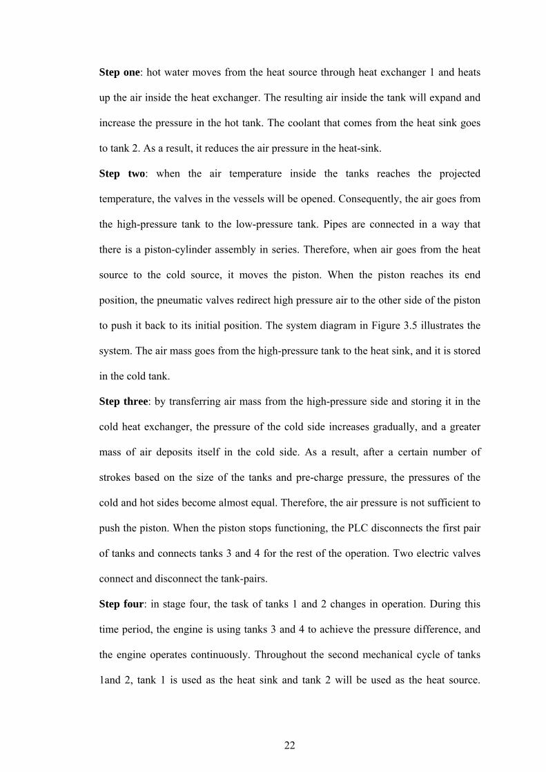
Figure 3.5a: Shell and tube heat exchanger with helical coils. .................................... 27
Figure 3.5b: Shell and tube heat exchanger with multi-pass coils. .............................. 27
Figure 3.6: Photo of the shell and flanges in the MHE, with dimensions. .................. 28
Figure 3.7: Helical and multi-pass heat exchangers. ................................................... 29
Figure 3.8: Tube deformation in helical coils. ............................................................. 30
Figure 3.9: Two-way piston assembly in the MHE (modified from [59]). .................. 32

x
Figure 3.10: Comparison of torque outputs of two piston assemblies with different
diameters [59]. ............................................................................................................. 34
Figure 3.11: Ball valves (a) PVC ball valve and 4 RPM electromotor, (b) Iron ball
valve with electromotor and speed controller. ............................................................. 35
Figure 3.12: Pneumatic ball valves to change the air direction through the piston
assembly. ...................................................................................................................... 36
Figure 4.1: Schematic of a MHE with one pair of tanks for thermodynamic analyses;
section (a) is for the charging period and section (b) is for the discharging (operation)
period. .......................................................................................................................... 39
Figure 4.2: Schematic of tank1 with a water system boundary. .................................. 44
Figure 4.3: Schematic of the two-way piston cylinder assembly. ............................... 48
Figure 4.4: Comparison of Carnot cycle and Marnoch cycle. ..................................... 51
Figure 4.5: Five power-cycles of the MHE for five piston revolutions. ...................... 52
Figure 5.1: Maximum pressure differences with varying pre-charge pressures .......... 65
Figure 5.2: The variation of created pressure differences in MHE with different initial
pressures ....................................................................................................................... 66
Figure 5.3: Relation of pressure differences with heat source temperatures ............... 66
Figure 5.4: Pressure variations in one pair of heat exchangers during the operation
period. .......................................................................................................................... 69
Figure 5.5: Total power output from the generator at varying pressure differences. .. 71
Figure 5.6: Total power output from the piston assembly at varying pressure
differentials. ................................................................................................................. 71
Figure 5.7: Measured power output from the generator from one tank pair at varying
pressure differentials. ................................................................................................... 72
Figure 5.8: Comparison of measured and predicted power outputs from the generator

xi
for varying pressure differentials during one operation cycle. .................................... 73
Figure 5.9: Comparison of measured and predicted peak power outputs from the
generator for varying pressure differentials. ................................................................ 75
Figure 5.10: Variations of Carnot efficiency at different source temperatures. .......... 76
Figure 5.11: Variations of Carnot efficiency with different temperature ranges. ........ 77
Figure 5.12: Energy and exergy efficiency versus system pressure (TC=298.15 K and
TH=343.15 K). .............................................................................................................. 78
Figure 5.13: Plot of Energy and exergy efficiencies versus system pressure.
(TC=274.15 K and TH=289.15 K). ................................................................................ 79
Figure 5.14: Effect of increasing the initial pressure on the exergy efficiency of the
MHE. ............................................................................................................................ 79
Figure 5.15: Effect of increasing the heat source temperature on the energy and
exergy efficiency of the MHE. ..................................................................................... 80
Figure 5.16: Schematic of the transmission in the current system. ............................. 82
Figure 5.17: MHE with 8 tank pairs. ........................................................................... 84
Figure 5.18: Trend of power outputs of an MHE with (a) two and (b) multiple pairs of
tanks. ............................................................................................................................ 85
Figure 5.19: Required transmission system for three pairs of tanks. ........................... 86
Figure 5.20: Schematic of the MHE with separated electric generators. ..................... 87
Figure 5.21: MHE with external heat exchangers and hydraulic motor. ..................... 88
Figure 5.22: Hydraulic assembly of the MHE with internal heat exchangers. ............ 90
Figure 5.23: Power output of the MHE with accumulators and hydraulic motor. ....... 90
Figure 5.24: Preliminary assembly of the MHE with accumulators. ........................... 91

xii
Nomenclature
A = area [m2]
AD
c
C
=
=
=
angular distance [o]
specific heat capacity [J/kg.K]
constant
D = diameter [m]
f = force [N]
F
Ex
=
=
friction factor
exergy [J]
G = gravitational acceleration [m/s2]
h = head loss [m]
Jm = rotational mass moment of inertia [kg.m2]
k = loss coefficient
K = radius of gyration [m]
KE
L
=
=
kinetic energy [J]
Length [m]
m = mass [kg]
xiii
P = pressure [Pa]
Re = Reynolds number
RT
RPM
R
=
=
=
rotational time [s]
number of revolutions per minute
gas constant for dry air [J/kg.K]
SRDR = shaft rotation per revolution [o]
T = temperature [K]
V = velocity [m/s]
Vol = volume [m3]
X = piston length [m]
Z
= height [m]
= mass flow rate [kg/s]
Greek Letters
Γ = exergetic temperature factor
= torque (N.m)
= efficiency
Δ = change

xiv
Subscripts
0 = dead state (ambient condition)
1, 2,... = state 1, 2, ...
a = air
apl = all piston losses
d = destroyed
e = electric
fa = from air
fpc = friction between the sealing and the cylinder body
frp = friction between rack and pinion
fw = from water
gen = generated
i = point number
in = inlet
out = outlet
p = piston
Q loss = heat loss

xv
t = total
ta = to air
tw = to water
w = water
Acronyms
DAQ = Data Acquisition System
OCE = Ontario Centres of Excellence
OPA = Ontario Power Authority
UOIT = University of Ontario Institute of Technology
IDB = International Data Base
MHE = Marnoch Heat Engine
NSP = Number of strokes per minute
LTD = Low-temperature differential
PLC = Programmable Logic Controller
PVC = Polyvinyl chloride

1
Chapter 1:
Introduction
1.1 Energy and Its Importance
The population around the world is rapidly growing. Even though many countries
have initiated new policies to reduce this growth rate, which averages 2% per annum,
the issue still persists [1]. It is predicted that the population will double by the year
2050 [2]. This population growth will create a huge demand for energy. World energy
demand in 2003 had increased by 20% in comparison to the nineties. More than half
of the world’s energy was consumed by around 950 million people in industrialized
countries [3]. Oil has been considered as a major source of energy ever since. Total
world oil demand is expected to increase from 77 million barrels in 2003 to about 119
million barrels in 2025, a 55% increase [3]. Uneven distribution of world resources
and the resulting dependence of many countries on politically unstable nations, raise
concerns about energy security [3].
In 2004, a research study by the Pembina Institute in Canada showed that
electricity consumption during peak hours by the year 2020 could be reduced to 30%
below the 2004 levels, through a series of energy efficiency and demand reduction
policies [4]. Energy is one of the key needs of modern society. Since the Industrial
Revolution, developed nations have primarily relied on fossil fuels for their energy
needs. This fossil fuel consumption has contributed to environmental pollution and
carbon dioxide emissions. Carbon dioxide comprises 82.3% of greenhouse gases and
it is considered to be the main greenhouse gas, which is linked to climate change and

2
global warming [5]. Furthermore, there are limited fossil fuel resources in the world,
which will eventually be exhausted [6].
Global warming is a major issue that has to be considered in regards to energy
production. Clean and sustainable energy resources are now preferable, together with
the more efficient use of fossil fuels. Renewable energy resources are one of the most
promising solutions for this energy demand. World contributions of coal, oil, gas,
nuclear and biomass in the current energy supply are shown in Figure 1.1. From this
figure and information from the International Energy Agency (IEA), more than 60%
of the total required global energy is being supplied by fossil fuels [7]. These statistics
differ from one region to another. For instance presently, the USA is nearly as
dependent on fossil fuels (85% in 2007) as it was 93% in 1973 [8].
Figure 1.1 shows significant continual growth of nuclear energy after year
2020. Nuclear technologies have been safe and reliable when used with precaution.
Some countries may be unwilling to employ nuclear power on a larger scale [9]. The
demand for these nuclear power plants and their capacity has to be increased, to
satisfy our ever growing energy demands. Since nuclear power plants require large
amounts of water for cooling, the majority of these power plants are built beside
lakes, rivers or seas. Hence, this water that cools the reactors will be drained to the
surroundings. As a result, it increases the surrounding temperature and has effects on
natural habitats [11]. One strong benefit of nuclear fuels is their high energy content.
This energy is generated during the nuclear fission process. This process is initiated
by a chain reaction using Uranium fuel. A nuclear reaction with U-235 releases more
than 1.6 million times as much energy per gram in comparison to a chemical
oxidation reaction of CH4 [12].

3
Figure 1.1: Distribution of energy from 1990 to 2095 (from [10]).
Figure 1.2: World electricity generation by source of energy (from [13]).
04000
8000
12000
16000
20000
Tera
wat
t hou
rs (
TW
h)
Others
Hydro
Nuclear
Gas
Oil

4
Figure 1.2 illustrates the world electricity generation by fuel type. The lowest
region in the figure shows that coal power plants have a steady and vital share of
electricity production in the world. The amount of coal in some countries like China
and the United states is abundant and their energy demand is high, thus, these
countries are building new coal power plants to meet this energy demand in the
future. Coal power plants are the single largest source of some of the worst air
pollutants, including deadly particulate matter, acid-rain-formation by sulfur dioxide,
and toxic mercury [14]. In power plants, several methods are being applied to increase
the efficiency and also capture released greenhouse gasses. In order to increase the
efficiency of these power plants, one way is to apply combined power generation
cycles. This solution can increase the efficiency of these plants by almost 60% [15].
Another method to increase the power plant efficiency is to operate these power
plants under higher pressures and temperatures, in comparison to conventional power
plants [16, 17]. An example of a power plant working over the normal regulated
pressure and temperature conditions is a power plant called the AD700 in Europe
[18]. Commencement of this project AD700 took place in 1998 in Europe. In cases
like these, the efficiency of a steam power plant can reach up to 55% [18]. Safety is
one of the main concerns regarding these projects. Most of the advanced materials
that are used incur large expenses and are hard to fabricate. Examples of such
materials are different stainless steels, Inconel alloys, high-temperature ceramics, and
coatings [19, 20]. Engineers have been trying to develop the most appropriate material
for such projects. However, corrosion is still one of the main concerns in power plants
[21, 22]. By increasing the efficiency of a power plant by even one percent, it can
have significant gains for the reduction of greenhouse gas emissions to the
environment.

5
Another process for reducing greenhouse gases is to use alternate renewable
sources of energy. In the transportation sector, this can be achieved by electric
vehicles powered with batteries, fuel cells on board, the combination of internal
combustion engines with renewable energy sources in hybrid cars, or in aircraft [23,
24]. By using renewable sources of energy, it will be possible to generate the
electricity in large quantities, to power different sectors of society. The most common
renewable energy systems are hydroelectric, solar panels, wind turbines, tidal
turbines, and geothermal heat sources.
Wind energy is a prime example of a sustainable energy resource. Because it
is a non-polluting source of energy during power generation, it has no emissions or
residues to burden society. However, it is limited by its site and intermittency; it
stands out as a viable alternative to fossil fuels [25]. Some analysts estimate that wind
energy will be limited to a maximum of 20% of the total installed generating capacity
from all sources. Its role would be confined to displacing higher cost fossil fuels for
electric generation [26].
Oceans are a major source of mechanical and thermal energy. Their energy
can be converted to electricity using different methods. Ocean mechanical energy is
quite different from ocean thermal energy. Even though the sun affects all ocean
activities, tides are primarily driven by the gravitational pull of the moon and waves
are driven by the winds. A barrage is typically used to convert tidal energy into
electricity by forcing the water through turbines, thereby driving a generator. In
favourable locations, wave energy density an average is 40 MW per kilometre of
coastline [27].
Renewable sources of energy are not uniformly available everywhere. Some
power generation systems like fuel cells are expensive and heavy in some applications

6
[28]. Fluctuations of energy sources in some cases are so high that we cannot rely on
these resources for critical usage. Some of them require huge capital costs and it takes
many years to repay that investment. For this reason, some countries stay with their
old energy systems for power production. Hence, one of the best solutions to solve the
problem of energy demand and pollution in the world is to increase the efficiency of
major power generation systems like power plants. This is possible by effective use of
energy recovery systems.
1.2 Motivation and Objectives
Marnoch heat engine can be used as an individual energy system or as a heat recovery
system for producing green energy. Currently, there is a great demand for research
and development of heat engines, which can produce electricity in industrial scales.
Increasing the amount of electricity produced by the heat engines and their lifetime
are two main goals of the researchers in this area.
This thesis performs a comprehensive thermodynamic performance investigation
of the current Marnoch heat engine at UOIT. The main objectives of thesis are (i)
energy and exergy analyses of the MHE, and (ii) experimental performance and data
acquisition.
Furthermore, suggestions are made for the mechanical configuration of the
future MHE prototype by using different components such as multiple tank pairs, and
hydraulic systems.
7
Chapter 2:
Literature Review
Heat recovery systems recover the heat during exchange with other systems. In some
cases, it converts and captures the heat in different forms of energy such as electricity.
Energy recovered from such systems can be used after its recovery, or it can be stored
for use during peak periods. In a number of other applications, cold thermal energy
storage is applied for energy savings [29].
Energy recovery systems exist in several forms. In one method, energy is
recovered in the form of compressed air [30, 31]. Compressed air energy storage
gives the opportunity to increase the efficiency of wind powered energy systems.
Such a recovery system stores energy, when in excess and subject to availability. It
can then be used as backup during energy consumption peaks [32].
With pumping storage systems, it is possible to store energy at a lower
consumption rate by pumping water onto an elevated reservoir during off-peak hours.
During peak hours, hydropower energy can be produced by the release of this water to
a lower level reservoir through a water turbine [33]. In such a pumping storage system
cycle, electricity is converted to mechanical energy and back again to electricity.
During these processes, some part of the stored energy is lost because of
irreversibility within the energy conversion and storage systems.
Another category that can be used as a heat recovery system to produce
electricity is heat engines. These systems can produce electricity using temperature
differentials. In the next chapter, different heat engines and their operation will be
discussed in detail.

8
2.1 Background
A heat engine system converts thermal energy to mechanical energy, using
temperature gradients between the heat source and the heat sink. Cengel and Boles
[34] outlined four main characteristics of heat engines as follows:
1. Heat engines receive heat from a high-temperature source.
2. These engines convert part of the heat to work (usually in the form of a
rotating shaft).
3. They reject the remaining waste heat to a low-temperature sink
(Environment).
4. They operate on the basis of a power-cycle.
The term heat engine is often used in a broader sense to include work-
producing devices that operate in a thermodynamic cycle. Engines that involve
internal combustion such as gas turbines and car engines fall into this category. These
devices operate in a mechanical cycle, but not a closed thermodynamic cycle. The
working fluid (combustion gases) in these heat engines do not go through a complete
cycle. In these systems, instead of cooling the exhaust gases, fresh gas originates
within the system.
All thermodynamic systems require a working substance. Generally working
fluids are considered as the fluids moving through the equipment, often as gases.
These gases can expand and compress easily. Common examples of working fluids in
a thermodynamic system are air, steam and hydrogen.
Daley [35] reported that hydrogen, as a working fluid, permits the most
compact engine design among any other working fluids (for a given power output and
efficiency). Therefore, hydrogen has been the choice of Stirling development
programs for automotive applications where engine size is a major concern. Daley
9
[35] stated that, systems using helium or air as a gaseous working fluid can be used
where size is not an important factor.
Due to the molecular weight and size of hydrogen, those systems which use
hydrogen as a working fluid have to be well contained. Hydrogen molecules can
penetrate through most containment vessels that are available [36]. Air in the form of
a working fluid has certain limitations, like poor heat conductivity as compared to
hydrogen, in heat engines [37]. However, air as a working fluid is more preferable in
many systems because it is freely available and it is not reactive.
2.2 Gas Power Cycles
Some important gas powered cycles are discussed in this section. Most gas power-
cycles were originally developed in the nineteenth century [38]. Table 2.1 shows
comparisons of processes for twelve different gas power-cycles.
These power-cycles consist of compressions and expansions of working fluids.
The working fluid in a cylinder can be compressed by pushing a piston.
To calculate the work output from a heat engine system, the cyclic-work has to be
calculated. Typically, gas power-cycles consist of four processes [39].
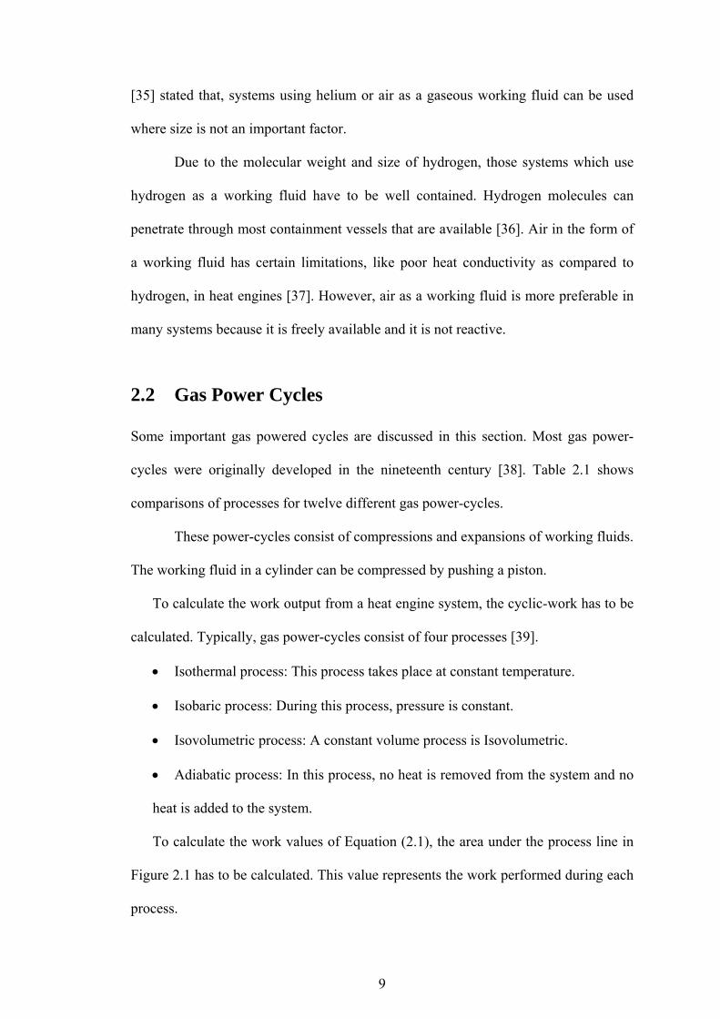
Isothermal process: This process takes place at constant temperature.
Isobaric process: During this process, pressure is constant.
Isovolumetric process: A constant volume process is Isovolumetric.
Adiabatic process: In this process, no heat is removed from the system and no
heat is added to the system.
To calculate the work values of Equation (2.1), the area under the process line in
Figure 2.1 has to be calculated. This value represents the work performed during each
process.
10
Figure 2.1: Four main thermodynamic processes in power-cycles.
2.2.1 The Carnot Cycle
In this section, essential details about the Carnot cycle are illustrated. This cycle is an
ideal cycle and cannot be achieved in practice. Figure 2.2 shows the power-cycle of a
Carnot heat engine. In a Carnot cycle, the system executing the cycle undergoes a
series of four internally reversible processes. This includes two adiabatic processes
and two isothermal processes.
Table 2.1 defines the steps for a Carnot heat engine. During the isothermal
expansion process 3-4, referring Figure 2.2, the temperature of the reservoir is
constant, and to keep this process reversible, the temperature difference between the
heat reservoir and gas is small. The same condition exists for process 1-2 in Figure
2.2. In this process, isothermal compression takes place. The amount of heat that is
being absorbed by the heat sink has to be exactly equal to the heat generated as a
result of compression. Process 2-3 shows that the gas is compressed adiabatically.
Process 4-1 in Figure 2.2 shows that the system is insulated, and the gas is allowed to
continually expand adiabatically until the temperature reaches the heat sink
temperature.

11
Table 2.1: Comparison of processes for different gas power-cycles
Cycle name Process 1-2 Process 2-3 Process 3-4 Process 4-1
Atkinson cycle Constant pressure Adiabatic Constant Volume Adiabatic
Brayton cycle Isobaric Adiabatic Isobaric Adiabatic
Cayley cycle Constant Pressure Polytropic Constant Pressure Polytropic
Carnot cycle Isothermal Adiabatic Isothermal Adiabatic
Crossley cycle Polytropic Constant Volume Polytropic Constant Volume
Diesel cycle Adiabatic Constant Pressure Adiabatic Constant Volume
Ericsson cycle Constant Pressure Isothermal Constant Pressure Isothermal
Otto cycle Adiabatic Constant Volume Adiabatic Constant Volume
Rankine cycle Isentropic Isobaric Isentropic Isobaric
Reitlering cycle Isothermal Polytropic Isothermal Polytropic
Stirling cycle Isothermal Constant Volume Isothermal Constant Volume
Stoddard cycle Adiabatic Constant Pressure Adiabatic Constant Pressure
Source: [38, 40]
In each of the four internally reversible processes of the Carnot cycle, work
can be represented by the enclosed area in Figure 2.2a. The areas under process lines
3-4 and 4-1 show the work done per unit mass by the gas, as it expands in these
processes. The areas under curves 1-2 and 2-3, show the required work for
compression in a Carnot cycle.
Figure 2.2: Carnot cycle (a) P-V diagram; (b) T-s diagram.

12
Figure 2.3: Stirling cycle (a) P-V diagram; (b) T-s diagram.
2.2.2 Stirling Cycle
The Stirling cycle is a well known power-cycle that represents the processes in a heat
engine. A Stirling cycle uses a regenerator in its cycle. Figure 2.3 shows the related P-
V and T-s diagrams for a Stirling cycle. This cycle consists of four internally
reversible processes in series: isothermal compression from state 1 to state 2 at the
heat sink temperature, constant volume heating from state 2 to state 3, isothermal
expansion from state 3 to sate 4 at the heat source temperature, and constant volume
cooling from state 4 to state 1. All heat addition and rejection during processes 3-4
and 1-2 occur in the isothermal processes [41].
2.3 Stirling Engines
The Stirling engine was invented by Robert Stirling in the year 1816 [42]. Its purpose
was to function as a safer source for generating power than the steam engine. Steam
engines had a common problem of having their hot water boilers explode from
extreme buildup of pressure. During that time, Stirling engines were used for water
pumps and fans. In the late 1800s they had become quite popular due to the fact that
they were so dependable, safe, and easy to use [43]. The early 1900s brought a decline

13
for the Stirling engine as engines running on cheap fossil fuels appeared. In the 1940s
and 1950s as gas prices rose, engineers started to see the first environmental effects of
fossil fuel engines, so research and development on heat engines started again [44].
One of the most important features of a heat engine is that many fuel sources
can be used to operate them. They can use renewable energy sources as solar energy.
For example, some Stirling engines that are being used in the United States are using
solar energy, or when there is not enough energy available, they can use methane
instead [45]. Another advantage of using a heat engine is its silent operation. In
comparison to Internal Combustion Engines (ICE), heat engines are almost noiseless,
since combustion does not need to take place inside the engine and compression ratios
are generally less than that of ICEs. Below, some of the advantages and disadvantages
of heat engines are listed.
Advantages:
Heat engines can operate quietly.
Heat engines can be environmentally clean, because they can operate on
all type of heat sources.
Heat engines can be made of cheaper materials than the other methods.
Disadvantages:
A requirement of heat engines is a heat source that is continually available
and has almost a constant temperature.
Heat engines cannot start and stop running as fast as ICEs, thus their usage
in vehicles would be ineffective.
The weight and volume of heat engines, in comparison to ICEs that
produce the same amount of power, is generally large.
It can be concluded that Stirling engines have the capability to be used in
many applications and it is suitable in the following cases [45].

14
Multi-fuelled characteristics are required.
A very good cooling source is available.
Quiet operation is required.
Relatively low-speed operation is permitted.
Constant power output operation is permitted.
Slow changing engine power output is permitted.
A long warm-up period is permitted.
2.4 Different Configurations of Stirling Engines
Four types of Stirling engines are discussed in this section. Based on the availability
of the heat source and sink, and simplicity, one of these configurations can be
selected. These configurations do not show the designs in detail, but just the key parts
are shown in the sketches. In Stirling engines, expansion and compression takes place
in a cylinder with a power piston. When they are operating, a displacer transfers the
working fluid through the heater, cooler, and regenerator.
2.4.1 Alpha Configuration of the Stirling Engine
Figure 2.4 shows the Alpha configuration of Stirling engines. This assembly has no
displacer involved, and the two pistons are working together so that the volume stays
constant.
Cold and hot pistons move uniformly in the same direction and they provide
constant volume heating and cooling processes of the working fluid. When the
majority of gas is in one cylinder, the other piston expands and compresses the
working fluid. Expansion takes place on the hot side, and compression occurs in the
cold side [45, 47].
15
Figure 2.4: Schematic of the Alpha configuration of the Stirling engine (modified from [46]).
2.4.2 Beta Configuration of the Stirling Engine
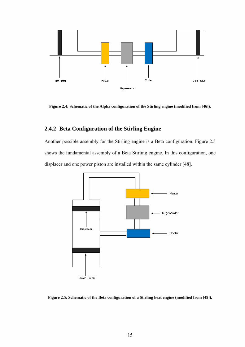
Another possible assembly for the Stirling engine is a Beta configuration. Figure 2.5
shows the fundamental assembly of a Beta Stirling engine. In this configuration, one
displacer and one power piston are installed within the same cylinder [48].
Figure 2.5: Schematic of the Beta configuration of a Stirling heat engine (modified from [49]).

16
In the Beta assembly, the working fluid between the heat source, sink, and
regenerator is moved by the displacer. The power piston and heat sink are located in
the same place in the Beta configuration. It compresses the gas when the working
fluid comes to the heat sink, and the gas expands when the fluid is moved to the heat
source.
2.4.3 Gamma Configurations of the Stirling Engine
Unlike Beta heat engines, in the Gamma configuration of heat engines, two separated
cylinders, one for the displacer and the other for the power piston, are used [50].
Figure 2.6: Schematic of the Gamma Configuration of the Stirling engine (modified from [49]).
Figure 2.6 shows the fundamental assembly of this heat engine. The
configuration and components of this heat engine are similar to the Beta
configuration; however, there are numerous differences in mechanical assemblies.
17
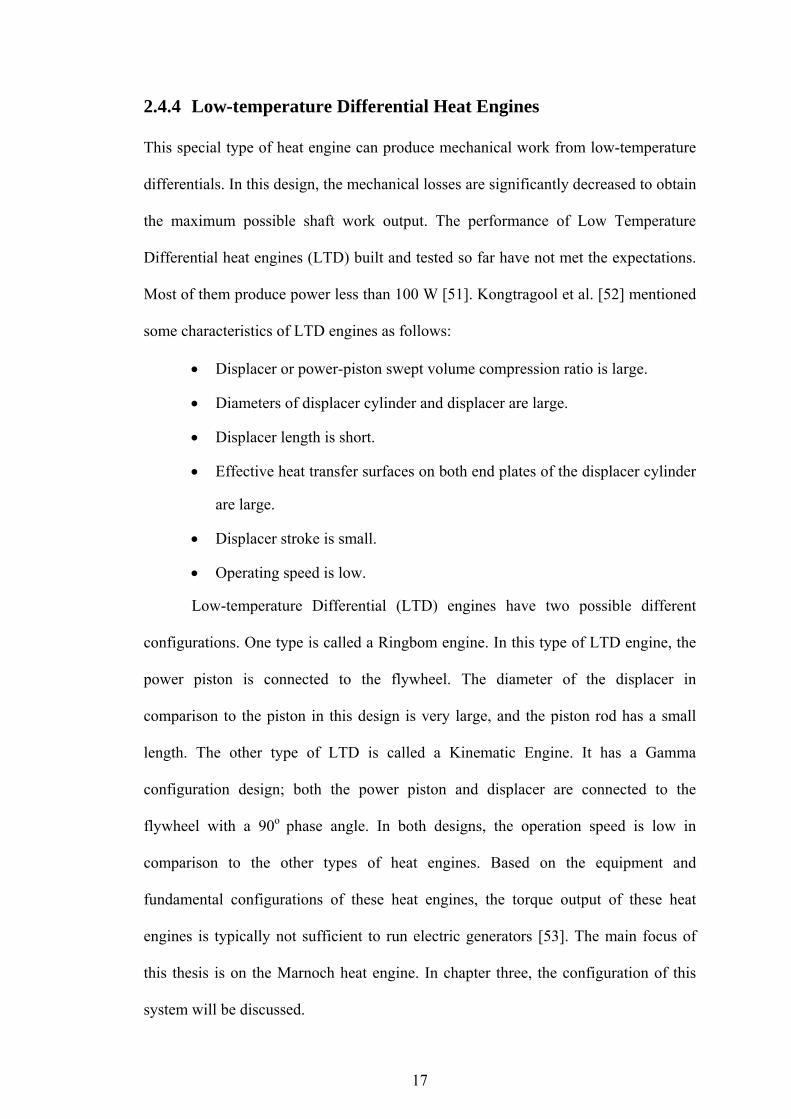
2.4.4 Low-temperature Differential Heat Engines
This special type of heat engine can produce mechanical work from low-temperature
differentials. In this design, the mechanical losses are significantly decreased to obtain
the maximum possible shaft work output. The performance of Low Temperature
Differential heat engines (LTD) built and tested so far have not met the expectations.
Most of them produce power less than 100 W [51]. Kongtragool et al. [52] mentioned
some characteristics of LTD engines as follows:
Displacer or power-piston swept volume compression ratio is large.
Diameters of displacer cylinder and displacer are large.
Displacer length is short.
Effective heat transfer surfaces on both end plates of the displacer cylinder
are large.
Displacer stroke is small.
Operating speed is low.
Low-temperature Differential (LTD) engines have two possible different
configurations. One type is called a Ringbom engine. In this type of LTD engine, the
power piston is connected to the flywheel. The diameter of the displacer in
comparison to the piston in this design is very large, and the piston rod has a small
length. The other type of LTD is called a Kinematic Engine. It has a Gamma
configuration design; both the power piston and displacer are connected to the
flywheel with a 90o phase angle. In both designs, the operation speed is low in
comparison to the other types of heat engines. Based on the equipment and
fundamental configurations of these heat engines, the torque output of these heat
engines is typically not sufficient to run electric generators [53]. The main focus of
this thesis is on the Marnoch heat engine. In chapter three, the configuration of this
system will be discussed.

18
Chapter 3:
The Marnoch Heat Engine
This chapter presents a study of the performance and operation of a Marnoch Heat
Engine (MHE) prototype unit. The main focus is heat recovery from low-temperature
heat sources.
3.1 Energy Conversion Steps and Processes
The Marnoch heat engine functions similar to the other heat engines and converts
thermal energy to mechanical work. In the MHE assembly, the mechanical work done
by the heat engine is converted to electricity. Figure 3.1 shows the steps of energy
conversion in a MHE.
The MHE is able to produce electricity from low-quality energy sources,
having temperatures less than 373.15 K. In this novel heat engine, heat exchangers are
installed at different locations from the piston cylinder assembly; hence, the heat can
be collected from various reservoirs [54, 55].
Figure 3.1: The working stages of energy conversion in a Marnoch heat engine.
Air in a Marnoch Heat Engine operates in the gaseous phase. It carries heat
from the heat source to a heat sink, and the working fluid passes through the piston
assembly of the heat engine and produces shaft work. This gas flow occurs as a result
of pressure differentials in hot and cold tanks. In comparison to other heat reservoirs,

19
and based on the availability of space for this type of engine structure, it is possible to
use a different working fluid in MHEs. The required heat for this system can be
supplied from power plants, solar energy or waste heat from various sources.
Moreover, in some regions, it is possible to use geothermal reservoirs to obtain the
required temperature differences [56]. Considering the available temperature
differences, it is possible to modify the mechanical design of the MHE to achieve the
highest possible efficiency within the system.
3.2 System Operation
This section gives an introduction to the current MHE and its patent [57]. Figure 3.2
shows the schematic of the system and Figure 3.3a is a photograph of the present
MHE.
The current prototype of the MHE has two pairs of heat exchangers with
helical coils made of copper tubes. All heat exchangers are connected to the heat
source and heat sink. Pneumatic valves control the air direction into the piston
cylinder assembly. Solenoid valves were employed to control the water direction from
the reservoirs, and the two electric valves are switching between the tank-pairs. A
two-way piston assembly with a rack and pinion is used to convert the energy of the
expanded gases into mechanical work. All the valve motions are controlled by a
Programmable Logic Controller (PLC).
A programmable controller is used for automation of the MHE. MHE motions
of the pneumatic valves are changed in less than one second, thus, one cannot operate
the engine manually. The Marnoch embedded system carries out a pre-defined task
repeatedly, while making decisions based on varying physical and logical control
parameters. C language software written for the Marnoch system resides on the ROM
(read-only-memory). The Marnoch control system was designed to require minimal

20
input from the user, so only signals from the pressure and temperature sensors are
primary control triggers. Data was processed using the 80 MHz processor, with an
address and data bus width of 16-bits.
The transmission system of this prototype converts the reciprocating motions
of the piston to a one-way rotary motion. In each movement of the piston, the piston
rack rotates the pinion 270 degrees. As shown in Figure 3.3b, using two chains, the
clockwise and counterclockwise motions of the system are converted to a one-way
clockwise rotary motion. A freewheel in the pulley-center makes the pulley rotations
continuous. The pulley is connected to an electric generator by a belt and pulley. The
generated electricity is stored in an ionic battery.
Figure 3.2: Schematic of the MHE configuration with two pairs of tanks (modified from [57]).

21
Figure 3.3: Photos of the (a) current prototype and (b) transmission.
Different mechanical configurations of the MHE can have effects on the
performance of the engine. In Chapter Six, based on the experimental and theoretical
results, some possible and modified designs for the next generation of heat engine will
be discussed.
3.3 Description of MHE
In this section, a description of the MHE is presented. First, operation processes will
be presented for each operation step. These steps are different from the processes of
the Marnoch cycle; however, the processes of the cycle can be defined from these
steps. Water is used to transfer heat from the heat source to the system and extract
heat from the working fluid in the unmixed-heat exchangers. Moving boundary-work
is converted to mechanical work by utilization of a two-way piston-cylinder assembly.
The steps of the mechanical operation are discussed below.
22
Step one: hot water moves from the heat source through heat exchanger 1 and heats
up the air inside the heat exchanger. The resulting air inside the tank will expand and
increase the pressure in the hot tank. The coolant that comes from the heat sink goes
to tank 2. As a result, it reduces the air pressure in the heat-sink.
Step two: when the air temperature inside the tanks reaches the projected
temperature, the valves in the vessels will be opened. Consequently, the air goes from
the high-pressure tank to the low-pressure tank. Pipes are connected in a way that
there is a piston-cylinder assembly in series. Therefore, when air goes from the heat
source to the cold source, it moves the piston. When the piston reaches its end
position, the pneumatic valves redirect high pressure air to the other side of the piston
to push it back to its initial position. The system diagram in Figure 3.5 illustrates the
system. The air mass goes from the high-pressure tank to the heat sink, and it is stored
in the cold tank.
Step three: by transferring air mass from the high-pressure side and storing it in the
cold heat exchanger, the pressure of the cold side increases gradually, and a greater
mass of air deposits itself in the cold side. As a result, after a certain number of
strokes based on the size of the tanks and pre-charge pressure, the pressures of the
cold and hot sides become almost equal. Therefore, the air pressure is not sufficient to
push the piston. When the piston stops functioning, the PLC disconnects the first pair
of tanks and connects tanks 3 and 4 for the rest of the operation. Two electric valves
connect and disconnect the tank-pairs.
Step four: in stage four, the task of tanks 1 and 2 changes in operation. During this
time period, the engine is using tanks 3 and 4 to achieve the pressure difference, and
the engine operates continuously. Throughout the second mechanical cycle of tanks
1and 2, tank 1 is used as the heat sink and tank 2 will be used as the heat source.

23
Solenoid valves are changing the direction of water from the heat source and sink,
such that hot water goes to tank 2 and cold water goes to tank 1 during this cycle.
When the pressure inside tanks 3 and 4 is almost equalized, the first pair will be
reused to get the temperature difference, and step four is repeated for the second pair.
Figure 3.4: Connection diagram of the current prototype of the MHE with two pairs of tanks.
3.4 Comparison of Marnoch and Stirling Engines
In the earlier sections, the working principles of a Stirling engine and MHE were
presented. Thermodynamic and mechanical considerations show that there are three
major differences between the Stirling engine and the MHE.
24
1. In Stirling engines, a part of the mechanical work output from the flywheel is
used in the compression process. However, in the MHE, all of the energy that
comes out of the piston assembly is transferred to the electric generator.
2. In MHEs, cylinders of the power piston and heat exchangers can be located
away from each other. However, in the Stirling engine designs, heat
exchangers and piston assembly are attached. This feature of the MHE results
in the ability to use a variety of sources to create pressure differences from
temperature differentials.
3. Unlike Stirling engines, in MHEs, after each stroke, the enclosed area of a P-V
diagram changes. This area is reduced because after each stroke, the expansion
pressure reduces and the compression pressure increases.
3.5 Materials of Construction for MHEs
An MHE can be designed to operate over different temperature and pressure ranges.
Moreover, as discussed earlier, different working fluids in an MHE can be used for
the system. Some gases like ammonia are corrosive. Therefore, if this gas is used, all
parts in contact with the working fluid should be stainless steel. Some other working
fluids, like hydrogen and helium, have very small molecules. Hence gas leakage can
occur through small gaps. This is one of the main concerns when the system is
operating at high pressures.
At high pressures and temperatures, the materials selection has a significant
role in the design and manufacturing process. Safety and durability of the system is
strongly dependent on the materials and their properties.
In MHEs, hot and cold heat exchangers are inter-changed after each cycle of
operation; hence they are subjected to thermal shocks. On average during one hour of

25
operation, each tank will be cooled down and heated up 20 times. In the current
assembly, the heat engine uses temperatures ranging between 273.15 K to 373.15 K,
and energy transfers into the system via water streams. Therefore, for this engine,
properties of materials within this temperature range are investigated. In addition, if
the heat engine is going to use higher temperatures, around 1000o K, materials like
ferrite can incur phase transformation. If phase transformation takes place in
materials, the properties of materials will change noticeably.
In the current prototype, polymeric and cupric hoses and joints are used for hot
and cold water streams. During the first few hours of system operation, there are no
leakages that occur in joints, but after several hours, water leaks were observed in
some connections, because of the significant differences in the coefficients of
expansion of the materials. Common Teflon tapes are used for sealing joints of water
hoses, but for the working fluid section, gas piping seals are used. The same problem
is experienced during operation within air pipes. After several hours of operation, air
starts to leak from joints of electric valves and metallic hoses. Hence, it is preferable
to use materials having a similar coefficient of expansion for joints, hoses and valves.
3.6 Heat Exchanger Specifications
In the current configuration of MHE, four heat exchangers are used to heat up and
cool down the air inside the heat engine. Hot water from the reservoir flows through
two of the heat exchangers, and simultaneously cold water flows into the other two
heat exchangers. In each operation cycle, only one hot and cold heat exchanger is
operating.
The power generation of the system can be raised by increasing the heat
transfer rate within the heat exchangers. For instance, the water stream enters the

26
system with a temperature of T1 and increases the gas pressure from P1 to P2 in 60
seconds. If this time period is reduced to 45 sec, this pair of tanks can start the
operation 15 seconds faster. Thus, a certain amount of energy will be produced by the
heat engine within a shorter time period. Hence, the heat engine power output will
have higher values.
The design of the transmission in the MHE is strongly related to the volume
and heat transfer rates inside the heat exchangers. For example, if the applied heat
exchangers can tolerate high pressures, the speed of the piston can be higher in
comparison to low pressure units. Thus, the flywheel has to be heavier. In section 4.2,
calculations of the transmission system will be presented and the effect of each term
on the system performance is analyzed individually.
In this prototype, two different types of coils were used. For the first
prototype, helical tubes inside the shells were used. This configuration of coils has
two major advantages. Helical tubes can be fabricated easily. In addition, they have a
high heat transfer rate, inside a smaller required space, compared with the length of
the tubes.
In the second stage, the heat engine was rebuilt with multi-pass heat
exchangers. The same shells were applied in both earlier and later heat exchangers.
Figure 3.6 illustrates each configuration and shows the positions of installed valves
and sensors. Due to safety regulations, the air gauge pressure inside the shells cannot
be more than 1379 kPa in the present prototype. Reaching higher pressures at a
constant temperature inside the shells requires more gas inside the system. The heat
engine gives a higher torque output from the piston assembly with longer operation.
The effects of pressure variations on the performance of the system will be illustrated
in the thermodynamic analysis of the system in chapter four.
27
Figure 3.5a: Shell and tube heat exchanger with helical coils.
Figure 3.5b: Shell and tube heat exchanger with multi-pass coils.

28
Several heat exchanger configurations are possible in this design of heat
engine. Figure 3.6 shows a current photograph of the shells, which were used for the
helical and multi-pass coils. This figure shows the shape of the shells. Specific
dimensions of the shells and their flanges are available in Table 3.1.
Figure 3.6 shows the shell before insulation. After the heat engine assembly,
heat foil bubble insulation was used to insulate the heat exchangers. Figure 3.7 shows
the configuration of the coils inside the heat exchanger. As shown in Figure 3.7a, for
helical coils, two 90o elbows are used in the water tubes. Thus, in this configuration
the possibility of having leakages from the Copper tubes is not high.
Figure 3.6: Photo of the shell and flanges in the MHE, with dimensions.

29
Table 3.1: Shell side of seat exchanger specifications
Shell Diameter 330mm
Shell Length 790mm
Thickness of the Metal Sheet in the Body 4mm
Thickness of Flanges 23mm
Number of the Bolts that Tighten the Flanges 8
Bolts Diameters 22mm
Diameter of the Air Inlets and Outlets 25.4mm
Total Volume of the Heat Exchanger 0.07815m3
The challenge during fabrication of the helical section after rolling was tube
deformation. As a result of this deformation, the surface area of the tube was reduced
and flow rate of the water that comes through the tube was kept constant. Therefore,
the pressure drop increased because of the higher fluid velocity.
Figure 3.7: Helical and multi-pass heat exchangers.

30
As demonstrated in Figure 5.3a, another issue with the helical configuration is
that the coils are close to each other. Hence, air conduction from the inner part of the
coil to the outer part cannot occur easily. The average distance between each coil is
2.7 mm and some coils are joined together. To overcome these problems, another
design for helical copper tubes is illustrated in Figure 5.1b.
Figure 3.8: Tube deformation in helical coils.
In this configuration, 20 straight tubes were used and 38 short turn 90o elbows
were used to make the 180o turns. In the current system, the inner distance between
tubes is 25mm. Therefore, heat convection occurs faster than the previous
configuration of copper coils. The new diameter of tubes is increased to 14.6mm, and
after the fabrication process, no visible deformation took place within the tubes. Table
3.3 shows all related specifications of the multi-pass configuration.
In this step of the experiment, shells were not changed, and the flange inlet
diameter of the heat exchangers was 157mm. Therefore, no more than 20 straight
tubes could fit into each shell in the current configuration. To find the pressure drop
of water through the coils Bernoulli’s principle was applied. The pressure drop for the
water temperatures of around 4oC is about 5 kPa. This is small and it shows that the
pressure drop for water in the current system is not a major concern.

31
Table 3.2: Helical coil specifications
Tube Outer Diameter after Deformation a= 9.90mm, b=14.72mm
Thickness of Tube 0.64mm
Inner Diameter before Deformation 10.92mm
Outer Diameter before Deformation 12.20mm
Number of Coils 37
Length of Heat Exchanger Coils 630mm
Radius of Bends 65mm
Total Length of Tubes 17350mm
Total Occupied Volume by Tubes 2006.23(10-6)
Percentage of Occupied Shell Volume by Tubes 2.57%
Table 3.3: Straight pass tubes specifications
Thickness of Tube 0.64mm
Inner Diameter 14.61mm
Outer Diameter 15.90mm
Number of Passes 20
Length of Each Pass 690mm
Radius of Bends 22mm
Total Length of Tubes 15150mm
Total Occupied Volume by Tubes 3044.54(10-6)
Percentage of Occupied Shell Volume by Tubes 4.40%
32
3.7 Piston Cylinder Description
In the current prototype, a two-way piston cylinder assembly is utilized. The body of
the cylinder is made of aluminum. This aluminum is hard-coat anodized and
permanently sealed for wear resistance, and more endurance. The sealing in the
system is critical to avoid leakages from the piston assembly to the surroundings, and
from one side of the piston to the other side. At the same time, the friction loss
between the piston and cylinder must be minimized.
The piston in this prototype has the diameter of 63.30 mm. Figure 3.9 shows
the piston assembly and its elements. This assembly has a coupled rack and pinion
mechanism, and it is hardened by chrome in the alloy.
Figure 3.9: Two-way piston assembly in the MHE (modified from [59]).
In this equipment, the maximum operating pressure is 1723.7 kPa, with a
breakaway pressure of 34.5 kPa. Rotation of the shaft by each complete stroke is 270
degrees. The displacement per degree of rotation in the cylinder is 1.23 cm3.
Therefore, in each stroke, 331.83 cm3 of the working fluid is transferred to the low-

33
pressure tank. Seals in the piston are designed for continually running between
temperatures ranging from 255.45 K to 355.35 K [59].
The torque outputs of the piston-cylinder, in four pressure differences, are
shown in Table 5.1 for two different diameters. These values specifically belong to a
piston-cylinder with a diameter of 63.30 mm, which is currently used in the MHE.
These values are compared with the torque output from a piston assembly with a
diameter of 81.21 mm. They are proposed to be used in the next prototype.
As Table 3.4 shows, the higher torque output of the system requires higher
pressure differences. Based on the manufacturer’s specification of the piston, friction
losses in the assembly are about 20% of theoretical output torque. The actual torque
output of the piston in the specification sheet with a diameter of 63.3 mm, and
pressure difference of 689.47 kPa, is about 42.37 N.m [59].
Table 3.4: Torque output of the piston
Pressure Difference (kPa) 344.74 517.11 689.475 1723.69
Torque Output (N.m)
(Piston Diameter: 63.30mm) 24.29 36.38 48.58 121.35
Torque Output (N.m)
(Piston Diameter: 81.21mm) 64.40 96.04 128.92 322.23
Source: [59].
Figure 5.2 shows the variations between the torque outputs of a piston with
different diameters. The difference between the diameters of these pistons is 17.91
mm, and the differences between torque outputs are noticeable.
There are several aspects to be considered for piston sizing of the MHE. If the
volume of the cylinder is large, consequently the amount of working fluid that is
transferred from one tank to the other is high, per stroke. Hence, if the volume of the
heat exchangers does not match the piston size after a few of strokes, the engine

34
operation will be stopped and another pair of tanks must be charged for operational
use. The charging mode is time consuming, and delays in piston operation can happen
when tanks are being switched.
Figure 3.10: Comparison of torque outputs of two piston assemblies with different diameters [59].
An advantage of having cylinders with larger diameters and volumes is that
when a larger piston cylinder is used, less time is spent for changing the direction of
the piston by the valves. Thus, the power output from the piston assembly will have
higher values. Moreover, the torque output is more than the output of smaller pistons.
When smaller pistons are used, the direction is changed more frequently. Changing
direction by the valves is time consuming, thus certain amounts of energy are
produced in longer durations. Therefore, the output power of the piston will reduce.
0
50
100
150
200
250
300
350
0 500 1000 1500 2000
Torq
ue O
utpu
t (N
.m)
Pressure Difference (kPa)
Piston Diameter 81.21mm
Piston Diameter 63.30mm
35
The other concern about using large cylinders is the amount of required heat to
keep the process isothermal. For large volumes, this amount at the start and end of the
stroke is noticeably different. Practically, it is hard to keep the gas at the same
temperature in this condition for isothermal processes.
3.8 Control Valves
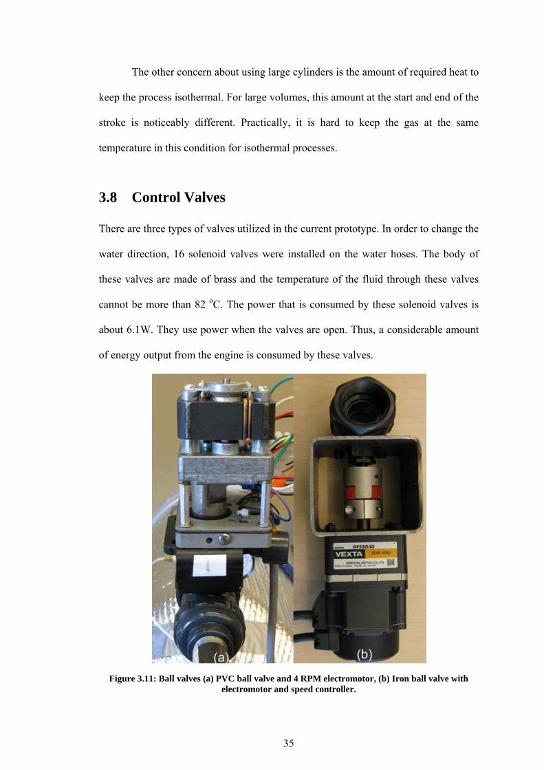
There are three types of valves utilized in the current prototype. In order to change the
water direction, 16 solenoid valves were installed on the water hoses. The body of
these valves are made of brass and the temperature of the fluid through these valves
cannot be more than 82 oC. The power that is consumed by these solenoid valves is
about 6.1W. They use power when the valves are open. Thus, a considerable amount
of energy output from the engine is consumed by these valves.
Figure 3.11: Ball valves (a) PVC ball valve and 4 RPM electromotor, (b) Iron ball valve with electromotor and speed controller.
36
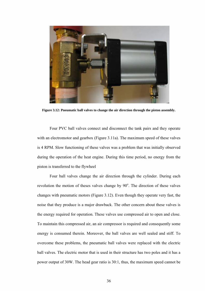
Figure 3.12: Pneumatic ball valves to change the air direction through the piston assembly.
Four PVC ball valves connect and disconnect the tank pairs and they operate
with an electromotor and gearbox (Figure 3.11a). The maximum speed of these valves
is 4 RPM. Slow functioning of these valves was a problem that was initially observed
during the operation of the heat engine. During this time period, no energy from the
piston is transferred to the flywheel
Four ball valves change the air direction through the cylinder. During each
revolution the motion of theses valves change by 90o. The direction of these valves
changes with pneumatic motors (Figure 3.12). Even though they operate very fast, the
noise that they produce is a major drawback. The other concern about these valves is
the energy required for operation. These valves use compressed air to open and close.
To maintain this compressed air, an air compressor is required and consequently some
energy is consumed therein. Moreover, the ball valves are well sealed and stiff. To
overcome these problems, the pneumatic ball valves were replaced with the electric
ball valves. The electric motor that is used in their structure has two poles and it has a
power output of 30W. The head gear ratio is 30:1, thus, the maximum speed cannot be

37
more than 100 RPM. These valves are connected to electric controllers. These
controllers change the valve speeds between 1 and 100 and control the required delays
during the operation.
38
Chapter 4:
Performance Analysis
4.1 Thermodynamic Analysis
Thermodynamic analysis is necessary to evaluate the performance of the MHE. All
major components of the MHE will be analysed separately, to determine the
parameters that have the most significant impact on the performance and efficiency of
the MHE. Thus, in future prototypes, particular attention will be given to these
parameters.
In order to perform a proper energy and exergy analysis on the MHE, a
boundary is defined for the system and its components. The time period for analyzing
this heat engine is also specified, since the same components perform different tasks
at different periods of the cycle. For instance, the first operation cycle operates for
about 29 to 60 seconds. Within this period, heat exchanger 1 transfers heat from the
hot reservoir and heats up the air inside the heat engine. At this time, tank 2 is
connected to the heat sink, and cools the air that is coming from the piston. Hence, if
this period is analysed, tank 1 and tank 2 are the heat source and heat sink,
respectively. In the next cycle, the functions of tank 1 and 2 will be reversed. In order
to present the analysis coherently, calculations for charging and discharging periods
of the heat exchangers are done separately.
The schematic of the system is shown in Figure 4.1. This figure represents the
first operation cycle in two different stages (charging and discharging). In Figure 4.1a,
both valves are closed and initially both tanks have the same pressure. When water

39
flows through the heat exchangers, tank 1 is heated to raise the pressure, and at the
same time, tank 2 is cooled and its pressure is decreased.
Figure 4.1: Schematic of a MHE with one pair of tanks for thermodynamic analyses; section (a) is for the charging period and section (b) is for the discharging (operation) period.
Figure 4.1b demonstrates the second step of the operation. In this step, the air
temperatures inside both heat exchangers are close to the temperatures of the water
streams. In step 2, air vales are open and this set of tanks and piston start the
operation. Operation of this set continues until the air pressures inside both heat
exchangers equalize. During charging and discharging periods, water flows through
the tanks continuously and it does not shut off until the last stroke. This occurs to
achieve near isothermal expansion and compression strokes of the piston.

40
In Figure 4.1, the setup and flow connections for one piston revolution is
shown. This figure is sufficient to conduct the thermodynamic analysis. However, for
continuous operation, all of the components shown in Figure 3.4 are required. In the
first part of the thermodynamic analysis, only the thermal energy balance is
considered, and the transmission system is analysed subsequently.
In this system, all properties of the working fluid are time dependent. It is
assumed that the water-flow from the reservoir is steady state. When the valves are
closed, it is assumed that no leakage takes place within the system, and air leakages
from the joints and hoses to the surroundings are neglected. Changes in volume of the
tanks, due to changes in heat exchanger temperatures and pressures are negligible, and
heat exchanger shells are assumed as rigid bodies. Fluid friction losses in the heat
exchangers are assumed to be negligible, and air is assumed to behave as an ideal gas.
In order to analyze the transient behaviour, the readings from the installed
sensors were used. The shortest period (dt) for the experimental readings cannot be
less than one second. In the theoretical analyses of the system, (dt) is the required
time for each revolution. This value is very close to one second in the current system.
The equations are solved by calculating the air properties after each stroke.
The three major components to be analyzed in the thermal energy analysis are
given as follows,
1. Tank 1: Connected to a heat reservoir;
2. Piston Assembly: A two-way piston assembly between the heat source and
sink;
3. Tank 2: Connected to a heat sink.
A general balance equation for any conserved quantity in a system can be written as:
Input + Generation – Output – Consumption = Accumulation (4.1)
41
Therefore, the general mass, energy, entropy, and exergy balance equations can be
written as:
Mass inflow – Mass outflow = Mass accumulation (4.2)
Energy inflow – Energy outflow = Energy accumulation (4.3)
Entropy input + Entropy generation – Entropy output = Entropy accumulation (4.4)
Exergy input – Exergy output – Exergy destroyed = Exergy accumulation (4.5)
In this analysis, Equations (4.2)- (4.5) will be used for each component separately to
conduct the thermodynamic analysis as shown below.
4.1.1 Mass Balance of Tank 1
Tank 1 is a shell and tube heat exchanger with both fluids unmixed. A heating fluid
(hot water) flows through the tubes and exchanges heat with the working fluid (air) in
the shell. The overall mass balance can be written as:
∆ ∑ ∑ (4.6)
Equation (4.6) is written separately for water as
∆ 0
(4.7)
Equation (4.7) shows that the water flow rate in tank 1 is steady state and the
mass of water inside the copper coils is constant. For air, the system is not at steady
state.
∑ , ∑ , ∆ (4.8)
As mentioned earlier in section 4.1, air leakages from the valves and joints are
negligible. In Equation (4.8), the values of the parameters for heating and cooling
modes for a set of tanks are equal to zero, because all air valves are closed, and no air
can enter and leave the tank. At the start of the piston operation, air leaves tank 1 and
no air mass will enter the tank. The air mass flow rate in Equation (4.8) for this
condition can be shown by negative values.
42
∆ (4.9)
where is the mass flow rate at point 5 (Figure 4.1) and it is a function of time. The
value of is calculated by Equation (4.10). After each piston stroke, the amount of
air mass that is transferred from the heat source to the heat sink decreases.
, (4.10)
The time step does not have a constant value even during one operation cycle. When
the pressures of both heat exchangers are equal, no air mass will be transferred from
tank 1, and again all parameter values in Equation (4.8) will be zero.
To perform the thermodynamic analysis, Uniform State Uniform Flow
(USUF) equations are used. In USUF processes, all properties are uniform within the
system at any instant in time. In addition, the flow is uniform so all mass flow
properties at each inlet and outlet are uniform. If tank 1 is assumed as a control
volume and the overall process occurs during time t , at any instant of time during the
process, the continuity equation is given by
, ∑ 0 (4.11)
where the summation is over all areas on the control surface through which the flow
occurs. In tank 1, only the exit point area is considered for Equation (4.11).
Integrating over t gives the changes of mass in tank 1 during the overall process:
, (4.12)
Where, denotes the initial air mass in tank 1, and denotes the
air mass that remains in tank 1 after one operation cycle.
Thus, the final and initial properties of the gas inside the heat exchanger allow
the value in Equation (4.12) to be calculated. This equation can be solved for the
whole period of the discharging process. To find the performance of the engine
43
between these periods Equation (4.11) is integrated over appropriate time periods,
Equation (4.13) shows this integration. The total mass leaving tank 1 during time (t1)-
(t2) is:
∑ ∑ (4.13)
Therefore, for the whole operation, over a period of time (t), the continuity equation
for the transient process can be written as:
∑ (4.14)
4.1.2 Energy Analysis of Tank 1
In the first cycle of operation, as shown in Figure 4.1, tank 1 is connected to the heat
reservoir. Equation (4.15) shows the general energy balance equation for this control
volume.
∆ ∑ ∑ (4.15)
This includes energy transfer by water streams and air. This equation is used
for tank 1 in two different modes: charging and discharging modes. In this equation,
∑ is the summation of total energy input to the heat exchanger 1, and ∑ is the
energy that leaves heat exchanger 1. In the first step, heat is transferred into the
system by the hot water stream. A portion of its energy is transferred to the gas inside
the heat exchanger. A fraction of ∑ goes back to the ambient by the exit water
stream, and the rest is lost to the surroundings. Figure 4.2 shows the system boundary
for the hot water stream that is entering tank 1. This figure is an illustration for
Equations (4.15) - (4.18).
Thus for the water stream:
(4.16)
here the values of and are obtained from Equation (4.6), and and

44
denote the enthalpy of the water that enters and exits the heat exchanger,
respectively. Thus, gives the flow rate of energy that is entering the system
by the water stream. The temperature of the water that is entering the system is
assumed to be constant during charging and operation. Hence, there will be no change
in the value of . Unlike , (energy flow to the ambient via
the outlet water stream) changes over time and its value depends upon (heat
transfer rate from the water to the working fluid). This rate is reduced over the period
of time during charging, because the temperature of the gas approaches the water
temperature. Also is the amount of heat that is rejected to the ambient from the
hot stream tubes, and it varies with time because the average temperature of the
stream changes with time. In the current system, the water temperature sensors are
positioned close to the tanks and the entire section is insulated. Thus, in the
calculations, can be neglected.
Figure 4.2: Schematic of tank1 with a water system boundary.

45
The heat transfer rate from the water stream to the air, in a given time, can be
expressed as:
∆ (4.17)
When Equation (4.17) is used for the charging period, the air mass (m) is
constant inside the tank, and its value is minitial in Equation (4.12). Temperature
differences shown by ∆T have major effects on the heat transfer rates. When this
equation is solved for the water streams, ∆T is the temperature difference between the
water inlet and exit, and the value of is the value of c at that specific temperature.
At the end of the charging period, the thermometers that are installed at the
water inlet and water exit do not show the same temperatures; however, after a certain
time, the pressure of the hot gas will remain constant. From the changes in
temperature and pressure, it is understood that the heat loss from the heat exchanger
to the ambient occurs, although the tank shell is insulated. When the piston operation
starts, considering Figure 4.1, it is assumed that
(4.18)
where T1and T2 are the water inlet and outlet temperatures respectively, and T5 is the
gas temperature inside the hot heat exchanger. It should be noted that heat loss from
the pipe, which connects tank 1 to the piston assembly, is neglected. Hence, air
temperatures at point 5 (Figure 4.1) and inside tank 1 are the same. This assumption is
appropriate in experimental conditions when the system is well insulated, or when the
ambient temperature is close to the hot stream temperature.
When the piston operation starts, heat is transferred by mass through the
piston assembly, and afterwards it is transferred into tank 2. When the air mass is
leaving the hot tank, the pressure of the tank will decrease. However, the expansion
process in this heat engine should be isothermal to obtain maximum work output.

46
Water flows through the heat exchangers during piston operation, so when the gas is
expanded, it is being heated up simultaneously.
The amount of heat that for the first revolution to keep the expansion
isothermal, is not equal to the required heat for the last expansion. In the current
system, the mass flow rate and temperature of the water that flows into the system is
constant. Hence, there is a variation between the actual expansions and isothermal
expansions, from theory.
The energy balance equation inside tank 1 during the operation mode can be
expressed as:
∆ (4.19)
where ∆ is the change in energy rates in tank 1 that occurs due to heat and mass
transfer. The value of is from Equation (4.17), is calculated in Equation
(4.10), and is the enthalpy of the air at the outlet.
4.1.3 Exergy Analysis of Tank 1
To find the performance of the system in different ambient conditions, an exergy
analysis was also performed. In the current system, no chemical reaction occurs with
air, or water that brings and removes heat from the system.
When no chemical reaction exists within the system, the physical exergy of
each point Exi can be calculated by:
(4.20)
where , and are enthalpy, temperature and entropy of dry air under ambient
conditions, respectively. Also and are the enthalpy and entropy at each point
within the system boundary.

47
If the tank is considered as a control volume, to find the flow exergy ),
which is associated with the heat transfer to the system , Equation (4.21) can be
used.
1
(4.21)
where is the incremental heat transfer, and the integral is taken from the initial
state (i) to the final state (f). This thermal exergy is the minimum work required by the
combined mass and environment in bringing the control mass to the final state from
the dead state. In the MHE prototype, in most of the conditions, heating the tank starts
from the dead state. But in situations where the temperature of the heat sink is lower
than the ambient, the initial state has negative values.
The dimensionless quantity 1
is called the exergetic temperature
factor, and denoted as [60]:
1
(4.22)
For heat transfer across a segment (r) of the control surface, for which tank 1
is charged initially, the thermal exergy associated with heat transfer is
. (4.23)
where qr is the heat flow per unit area at a region on the control surface, and the
temperature is denoted as Tr. The dimensions of the copper tubes inside the heat
exchanger are used to find the surface area (Table 3.2 and 3.3).
Equation (4.24) can be used instead of Equation (4.23) when the value of
is known. This equation gives certain values, whereby if the temperature T of the
control mass is constant, the thermal exergy transfer associated with the heat transfer
is:
1
Γ (4.24)
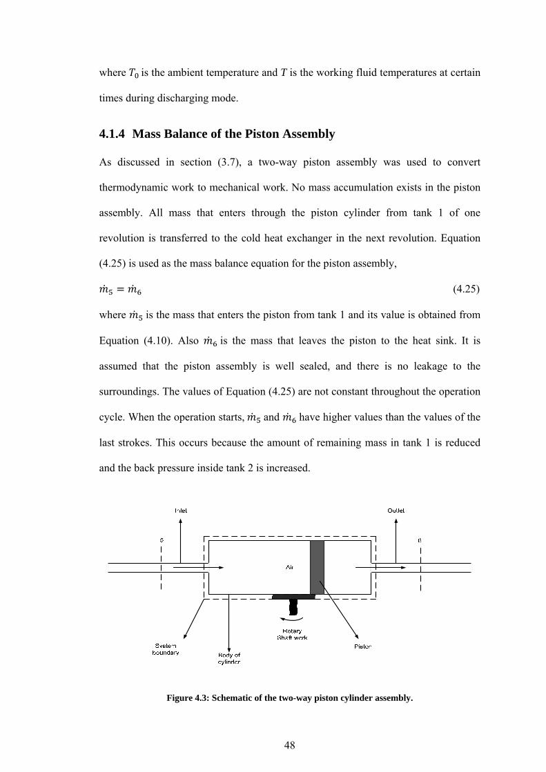
48
where is the ambient temperature and T is the working fluid temperatures at certain
times during discharging mode.
4.1.4 Mass Balance of the Piston Assembly
As discussed in section (3.7), a two-way piston assembly was used to convert
thermodynamic work to mechanical work. No mass accumulation exists in the piston
assembly. All mass that enters through the piston cylinder from tank 1 of one
revolution is transferred to the cold heat exchanger in the next revolution. Equation
(4.25) is used as the mass balance equation for the piston assembly,
(4.25)
where is the mass that enters the piston from tank 1 and its value is obtained from
Equation (4.10). Also is the mass that leaves the piston to the heat sink. It is
assumed that the piston assembly is well sealed, and there is no leakage to the
surroundings. The values of Equation (4.25) are not constant throughout the operation
cycle. When the operation starts, and have higher values than the values of the
last strokes. This occurs because the amount of remaining mass in tank 1 is reduced
and the back pressure inside tank 2 is increased.
Figure 4.3: Schematic of the two-way piston cylinder assembly.
49
4.1.5 Energy Analysis of the Piston Assembly
The piston assembly converts the heat exchanger pressure differences to shaft work.
Energy input enters by the expanded gas from the heat source, displaces the piston
and flows to the heat sink after work extraction. Equation (4.26) shows the energy
balance for the piston,
(4.26)
where is the total actual work output from the piston assembly, and is
the friction loss between the piston sealing and the inner body of cylinder. In the
current calculations, is a combination of static and dynamic frictions. This
friction loss is released in the form of heat and some fraction will be transferred to the
gas inside the piston, and a portion will be lost to the ambient. Also is the second
part of the friction loss. It occurs between the rack and pinion that converts the
revolutions to rotary motions. is the heat loss rate that is rejected from the gas to
the body of the cylinder, and afterwards to the ambient.
It is assumed that the temperature of the body of the cylinder is the average
temperature of the heat source and sink, because the inlet and outlet of the cylinder is
changed frequently. In the calculations for the piston assembly, , , and
were not calculated separately. All were considered as piston assembly losses ( ),
and values were found from the manufacturer catalogue. In the current setup this loss
is estimated between 10-20% of energy output of the piston assembly [59].
(4.27)
Substituting Equation (4.27) into Equation (4.26) gives
(4.28)

50
The installed pressure sensors on this heat engines has to respond in less than
one second. The reason is because of inlet and outlet of the piston change more than
50 times per minute. For instance, under 649.48 kPa of pressure difference, the inlet
and outlet switch occurs about 50 times in 58 seconds.
To find the shaft work output of the piston, the pressure differences in both
sides of the piston assembly were applied. From the pressure difference and piston
specifications, the torque output of the piston is obtained. By this method, the pressure
drops inside the valves and tubes are not considered in the calculation. It is a source of
error in the current experimental calculations.
4.1.6 Exergy Analysis of the Piston Assembly
Exergy that enters the piston cylinder assembly is carried by the air flow from tank 1,
and rejected to tank 2. To perform an exergy analysis, Equation (4.20) is used to find
the exergy at each point. With regards to Figure 4.1, it can be shown that:
(4.29)
where is the work extracted from the pressure differences. and are
the exergy of the air flow at the inlet and outlet of the piston, respectively. is
the exergy lost because of heat transfer to the ambient, and from one side of the piston
to the other side. is the exergy destroyed within the system from irreversibility.
The value of can be found by calculation of the entropy generation. The
relationship between entropy generation and exergy destroyed is defined as:
(4.30)
where is the irreversibility rate, is the ambient temperature and is the value
of entropy generated based on mass flow of the air in the piston assembly. Practically,
it is difficult to find the exact values for and separately, so in the

51
calculation, the combination of them can be used.
To find the work output per unit mass, both sides of Equation (4.29) should be
divided among the mass flow rate of the working fluid,
(4.31)
where is the shaft work output of the piston per unit air mass. Also and
are the exergy of the air flow through the inlet and outlet of the piston per unit
mass, respectively. Also shows all internal and external
irreversibilities per unit of working fluid mass.
4.1.7 Calculation of Shaft Work Output of the Piston Assembly
There are several ways to calculate the shaft work output from the piston assembly,
with regards to the current configuration of the MHE. As mentioned in the previous
section, one way to calculate the shaft work output is to find the gas enthalpy at
different points and performing energy and exergy analyses. The other way to find
this value is to focus on the thermodynamic cycle of the heat engine. The results of
the analysis will show how the system can be improved. In this section, the analysis
was performed by considering the thermodynamic cycle of the MHE.
P
V
3
4
2
1
Isothermal
P
V
3
4
2
1
Qin
Qin
Qo
ut
Qo
ut
W net. out W net. out
(a) (b)
Carnot Cycle Marnoch Cycle
Isothermal
Adiabatic
Figure 4.4: Comparison of Carnot cycle and Marnoch cycle.
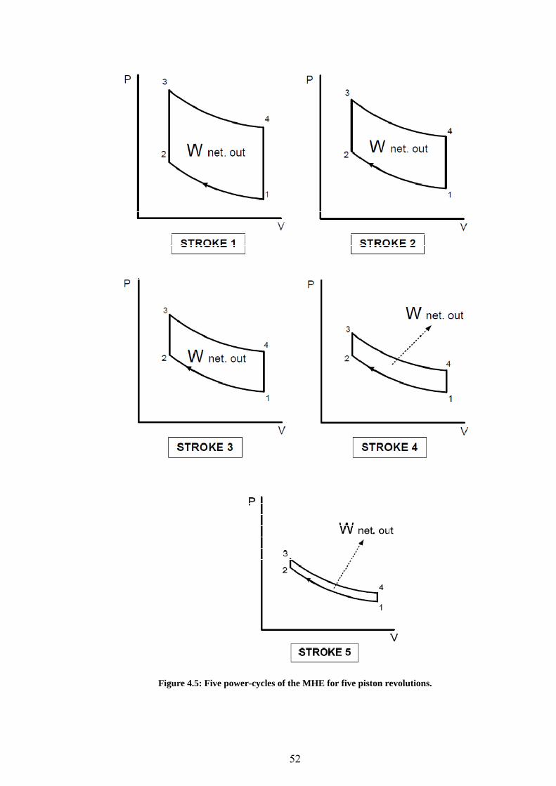
52
Figure 4.5: Five power-cycles of the MHE for five piston revolutions.
53
In Figure 4.4, the related thermodynamic power-cycle of the MHE [60] is
shown and compared with an ideal Carnot cycle. Figure 4.4b shows that the power-
cycle of the MHE is similar to the Stirling cycles. However, unlike the Stirling cycle,
the enclosed area of the MHE is reduced after each stroke during the operation of one
tank pair. Figure 4.5 is a demonstration of the area reduction of cyclic work output
from the piston assembly.
Pre-charge pressures and available temperature differences will affect the
number of piston revolutions, and relatively on number of power-cycles per operation
period. The following equations show how these variables change the performance of
the MHE.
As mentioned earlier, the compression and expansion processes in the MHE
are assumed isothermal and air is assumed to be an ideal gas. Thus, the ideal gas law
is used to find the air properties.
The MHE is a closed cycle; therefore no gas enters or leaves the system during
operation. The amount of leakage in the MHE is negligible; hence, the value of n is
constant. Thus, it is concluded that . Here C is a constant for each revolution.
By substitution of C in the ideal gas equation:
(4.32)
The work output of the piston as the result of one expansion can be found as:
(4.33)
Substituting (4.32) into (4.33) yields:
(4.34)
Thus:

54
∆ 1 ∆ (4.35)
The piston surface is constant during operation and during each revolution, but the
length is changed. Hence, ∆ ∆ . By using this value in Equation (4.35),
1 ∆ 1 ∆ (4.36)
Here is a constant that is defined as
Equation (4.36) shows the work output of the piston as the result of one
revolution. After the first revolution, some air mass is transferred to the other tank.
Thus, the pressure on the other side is changed and the value of C will be changed
accordingly. When the work output of the next stroke of the piston is calculated by
Equation (4.35), the work performed by the compression of the piston is negative.
After testing the engine several times and simulating different temperatures
and pressures, the time required for each revolution was found to be around 1 sec.
This timing will be evident in experimental graphs of power output in chapter five.
4.1.8 Mass Balance of Tank 2
When tank 2 is connected to the cold reservoir, water flows through the copper tubes
and cools down the air inside the heat exchanger. The air pressure inside the heat
exchanger drops. The thermodynamic analyses for this heat exchanger are similar to
the analyses for tank 1. The following analysis shows the main equations and
conditions in tank 2, when it is used as the heat sink.
In the present experimental setup, the temperature range of the heat sink is
between 282.15 K to 298.15 K. Similar to tank 1, tank 2 is an unmixed heat
exchanger. Water flows through the system at steady flow rates. Thus mass balance
equation for the water stream is given as:
(4.37)
55
The gas inside tank 2 is not in a steady state condition like tank 1. Thus,
Equation (4.8) can be applied to show the air mass balance. In this heat exchanger,
unlike tank 1 for the working fluid, in Equation (5.8), tank 2 ∆ ) has positive
values. The reason is because the air flows to the cold heat exchanger and
accumulates within this heat exchanger to be cooled down.
∆ (4.38)
Equation (4.25), for the piston assembly, shows that the mass accumulation in
tank 2 is equal to the mass leaving tank 1. Thus, similar equations are used for mass
balance of the working fluid in tank 2.
, (4.39)
Considering Equations (4.38), (4.39) and Equation (4.13), the total mass accumulation
in tank 2 is:
∑ (4.40)
When tank 2 is being charged, all values of Equation (4.8) are zero and no
mass flow exists in the system. When the operation starts, air accumulates in tank 2.
When the operation stops, no air transfers to tank 2. Air leakages from valves and
joints are neglected in the calculations. Similar to tank 1, to keep the compression
process almost isothermal, water flows through the system during the piston operation
period.
4.1.9 Energy Analysis of Tank 2
After leaving the piston, air will expand and its temperature will decrease. It will be
stored in heat exchanger 2. After multiple strokes, the working fluid pressure and
temperature in heat exchanger 2 starts increasing. Water from the heat sink goes
through the heat exchanger to cool down the air and decrease the temperature and
56
pressure. In the current calculations, it is assumed that the engine works continuously.
For the first step of operation of tank 2, the energy balance for a water stream of tank
2 in this step is defined as:
(4.41)
where and are the enthalpy of water at the inlet and outlet of the copper
tubes. Hence, is the energy of the water stream that enters the heat
exchanger, and its value is assumed to be constant with time. Also gives the
energy of the water stream that goes to the heat sink. It is decreases over the period of
time until the temperatures of water to the inlet and outlet of tank 2 are very close to
each other. represents the amount of heat absorbed by the water stream through
the heat exchanger. is the energy lost to the ambient from the air. When the
temperature of the heat exchanger is lower than the ambient, this value is negative
because heat is coming into the system. is negligible when the heat sink and
ambient have similar temperatures.
During the operation, heat transfer to the system occurs due to air movement
into the heat exchanger. The energy balance equation in this condition can be solved
for the water stream, or the heat exchanger shell as the system boundary. When the
area inside the shell is the system boundary, the heat coming to the system by air and
the heat removed by the exit-water stream are transient. A way to find the heat
removed from the system is to consider the heat exchanger copper tubes inside heat
exchanger 2, as the control volume.
∆ (4.42)
When the copper tube is the control volume, c is the specific heat capacity of water, m
is the water mass and ∆ shows the water temperature changes. When the water mass
flow rate is known, readings from the water inlet and outlet thermometers are used.

57
4.1.10 Exergy Analysis of Tank 2
The exergy balance equations for tank 2 are similar to the exergy equations for tank 1.
Equation (4.24) for tank 1 shows the exergy transfer from the water stream to the gas
due to heat transfer. However, in tank 2, exergy of the air will be transferred to the
water due to heat transfer. When the water stream in the copper tubes is used as the
control volume, the exergy balance equation can be written as:
0 (4.43)
where is the exergy of point 3 for the water inlet, and is the exergy of point 4
for the water outlet. These two values are calculated by Equation (4.20), considering
properties of water at these points. is the exergy associated with heat that is
transferred from the air to the water. The value of can be calculated from
Equation (4.21). Unlike heat exchanger 1, the value of in the calculations of tank
2 is either negative or close to zero. The reason is because the temperature of this tank
is either less than or close to the ambient temperature; hence, exergy associated with
heat will flow into the system.
4.2 Transmission System
In this section, the relative calculations of the transmission system are presented. The
equations are presented so it is possible to study the effects of applying different
piston and flywheel dimensions for the next MHE.
The information about the torque output for the piston used in the assembly is
available from the manufacturer’s catalogue. Based on the conditions for the piston,
losses from the piston can be different. The torque output for the series used in this
assembly is presented in Table 3.4. To find the rotational velocity of the piston, the
following correlation can be used:

58
(4.44)
where is the piston shaft rotation per minute, NSP is the number of strokes per
minute and SRDR is the shaft rotation degrees per revolution. In the current piston
assembly, the pinion rotates 270 degrees after each revolution, thus Equation (4.44)
can be written as:
0.75 . (4.45)
The rotational direction is changed after each piston revolution. To find the power
output for the piston, RPMP is multiplied by the torque output from the piston
assembly.
. (4.46)
where is the torque output of the piston assembly. Equations (4.44) and (4.46)
can be combined as follows:
(4.47)
Equation (4.47) calculates the power output from the two-way piston
assemblies. For this specific assembly, Equation (4.45) can be substituted into
Equation (4.46) to calculate the power output. in the MHE is changed after each
revolution, because the pressure differences after each stroke decrease. A way to find
the value of is to connect a torque meter to the piston assembly. In order to
estimate the power output from the piston assembly, the output kinetic energy from
the piston to the flywheel can be calculated. Considering the losses in chains and
bearings, the energy output from the piston can then be estimated.
In the current system, the thickness of the disc is negligible in comparison to
its diameter. Thus, to find the kinetic energy from the flywheel, Equation (4.48) can
be used:
59
. . (4.48)
where KE is the kinetic energy of the flywheel, Jm is the rotational mass moment of
inertia, and is defined as the angular velocity. To find Jm, Equation (4.49) is used,
. (4.49)
where W is the weight load, g is the gravitational constant, and k is the radius of
gyration. The value of to be substituted in Equation (4.48) is calculated by Equation
(4.50).
. 0.035 (4.50)
AD is the angular distance and Rt shows the rotational time. In the present setup, the
angular velocity of the flywheel was not measured. Thus, to find the kinetic energy of
the flywheel, it is assumed that the flywheel and piston are connected directly. Hence,
the AD value is 270o and the RT value is the required time for one revolution.
4.3 Efficiencies
There are different types of efficiencies that will be discussed in this section.
Theoretical and experimental data from the heat engine under pre-defined conditions
is obtained to calculate the system efficiencies.
4.3.1 Thermal (Energy) Efficiency of the Cycle
A limitation on the performance of the systems is indicated from the Kelvin-Planck
statement of the second law [41]. The thermal efficiency of the system can be defined
as:
(4.51)

60
where Wcycle is the work output of the cycle, and is the thermal efficiency of the
system (varies between 0-1). The variable can be calculated using Equation
(4.33). is the amount of heat entering into the system from the heat source. QH
can be defined in two different ways. In the first method QH is defined as the total
heat coming into the system from the hot water stream. In the second method, the QH
can be calculated by substituting , which is the amount of heat transferred to the
air, into Equation (4.51). The efficiency in the second method is independent of the
heat exchangers effectiveness, as well as losses in that section. Both methods will be
used to show the efficiency drop that occurs through the system because of the heat
exchangers.
4.3.2 Overall Efficiency of the Engine
The entire system performance can be evaluated, by the total efficiency of the system.
The final goal of the MHE is to generate electricity efficiently. Hence, in the
calculations, only the electric work from the generator is considered as the work
production. The overall efficiency of the system ( ) can be defined as:
(4.52)
where is the electric work output from the engine, and was discussed in section
4.1.2. has significant fluctuations, therefore, in order to have reasonable
calculations in the whole time period, the operation of one tank pair must be
considered for energy consumption and electricity generation.
4.3.3 Carnot Efficiency
The Carnot efficiency or ideal efficiency is the maximum possible efficiency of a heat
engine, when no irreversibility exists in the processes. Experimentally, reaching the
Carnot efficiency is not possible in heat engines. The Carnot efficiency gives a

61
prediction of the thermodynamic performance of the heat engine in varying
temperature ranges. The ideal efficiency of the MHE can be defined as follows:
1 (4.53)
where the values of and are the temperatures of the heat sink and heat source,
respectively.
4.3.4 Exergy Efficiency
The second law provides an indication of the irreversibilities within the system. The
amount of decrease in system performance due to heat and mechanical losses is
characterized by this law. In this study, the efficiency of the MHE based on the
second law is defined as:
п (4.54)
This can be calculated by substituting the overall efficiency of the engine and Carnot
efficiency into Equation (4.54). The efficiency can be increased by minimizing the
mechanical and heat losses within the system. For instance, these losses can be
minimized by preventing heat losses from the heat exchanger shells, and increasing
the heat exchanger performance.
The exergy efficiency is based on the second law of thermodynamics. The
exergy efficiency provides an alternative understanding of performance. In evaluating
the energy efficiency, the same weight is assigned to energy whether it is electric,
shaft work or low-temperature thermal energy. Exergy efficiency weights the energy
flows by accounting for each in terms of exergy [60]. From the exergy efficiency, it
can be understood how internal and external irreversibilities affect the performance of
the engine. The exergy efficiency ( ) for the MHE is defined as:
(4.55)

62
where is the exergy entering into the system. In this system, it is assumed that no
chemical reaction occurs in air as the working fluid. In the MHE, it is assumed that
the heat that entering the system is waste heat and no combustion is required to
generate this heat.
There are two ways to calculate . In the first method, the exergy of hot
water can be obtained from Equation (4.20) (point 5 in Figure 4.1). Thus, the value of
is the exergy of the hot water stream that goes through the hot heat exchanger. In
the second method, Equation (4.24) is used to find . Thus, is the exergy
transferred through the system associated with heat. Considering Equation (4.24), the
denominator of Equation (4.55) is smaller than the denominator of Equation (4.52).
Hence, the exergy efficiency of the system is higher than the system energy
efficiency. This can be explained by converting low grade energy in the MHE to high
grade energy of electricity.
4.4 Uncertainty Analysis
Uncertainty analysis is needed whenever an experiment is preformed, to determine the
errors associated with the experimental values. The uncertainty in the experimental
values has two components; bias and random variations. Bias is the error associated
with the inaccuracy of the measuring equipment, and it provides us with a measure of
the degree of closeness of the measured experimental values to the actual true values.
Random variations are the errors that occur due to the uncontrolled parameters when
making repeated measurements. They are related to the precision of the experimental
readings, and can be determined by finding the deviation of the readings.
63
The bias value for the experimental readings is equal to the accuracy of the
sensors used in the experiment, which are taken from the manufacturer’s catalogues.
Determining the random variations of the experimental readings requires finding the
standard deviation ( ), using the following equation:
∑ (4.56)
where is each individual experimental reading, is the mean value of the
experimental readings, and is the number of recorded experimental readings for
each variable. Then the precision can be found using the following equation:
(4.57)
To reduce the systematic errors, gauges were calibrated before carrying out the
experiments. The experiment was done several times for each set of data, and an
uncertainty analysis was carried out for each set of experiments. The main source of
inaccuracy is the measuring equipment. For example, the accuracy of the pressure
sensors is ± 6.9Pa, and the accuracy of the thermometers is ± 0.01ºC. The ambient
temperature during each test is non-uniform. For each case, the average temperature
of the surroundings was measured for the calculations.
The uncertainty (U) for experimental data is calculated by the following
equation:
√ (4.58)
where B is the bias limit, and P is the precision limit for the experimental readings.
64
Chapter 5:
Results and Discussion
In this chapter, the theatrical, predicted, and experimental results of the MHE are
presented. In the first section, effects of changing the pressures and temperatures on
the system are presented. By analyzing these results, it is possible to determine the
performance of the system in different conditions, and select the best components for
the heat engine.
5.1 Effects of Increasing the Pre-charge Pressure inside the
Tanks
Increasing the pre-charge pressure inside the tanks affects the structure and
performance of MHE. Moreover, raising this pressure will result in higher capital and
maintenance cost of the heat engine. Thus, to increase the pressure to higher levels,
proper economic and thermodynamic analyses need to be performed. Figure 5.1
shows how the pressure differentials vary with higher pre-charge pressures. Each line
in this figure belongs to a certain heat source and sink temperature. T1 is the initial
temperature and T2 is the final gas temperature. The trends of variations of pressure
differences in three different initial and final temperatures in the range of 273.15 K to
373.15 K are demonstrated. When the pre-charge pressure increases, at a certain
temperature (Figure 5.1), the same final temperature will result in higher pressures.
Hence, at low-temperature differences, high pressure systems have to be built to
obtain high enough pressure differences for continuous operation. Figure 5.2 shows
the variations of pressure differences in the MHE heat exchangers at different initial
pressures.
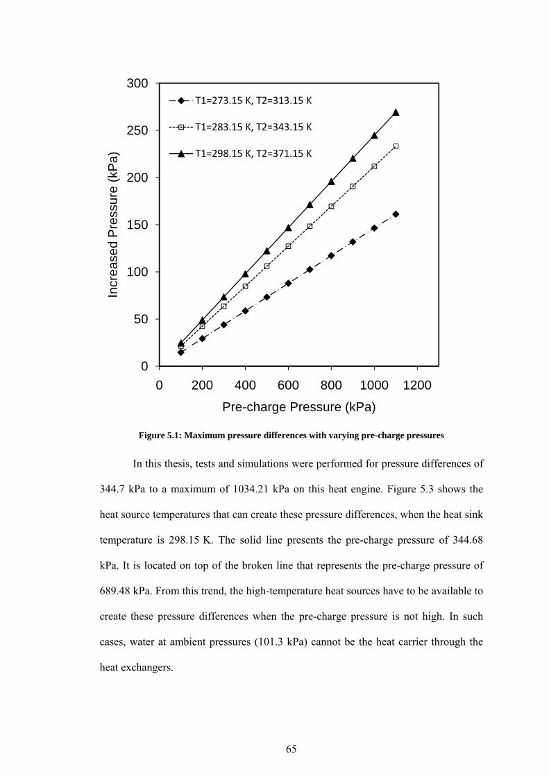
65
Figure 5.1: Maximum pressure differences with varying pre-charge pressures
In this thesis, tests and simulations were performed for pressure differences of
344.7 kPa to a maximum of 1034.21 kPa on this heat engine. Figure 5.3 shows the
heat source temperatures that can create these pressure differences, when the heat sink
temperature is 298.15 K. The solid line presents the pre-charge pressure of 344.68
kPa. It is located on top of the broken line that represents the pre-charge pressure of
689.48 kPa. From this trend, the high-temperature heat sources have to be available to
create these pressure differences when the pre-charge pressure is not high. In such
cases, water at ambient pressures (101.3 kPa) cannot be the heat carrier through the
heat exchangers.
0
50
100
150
200
250
300
0 200 400 600 800 1000 1200
Incr
ease
d P
ress
ure
(kP
a)
Pre-charge Pressure (kPa)
T1=273.15 K, T2=313.15 K
T1=283.15 K, T2=343.15 K
T1=298.15 K, T2=371.15 K
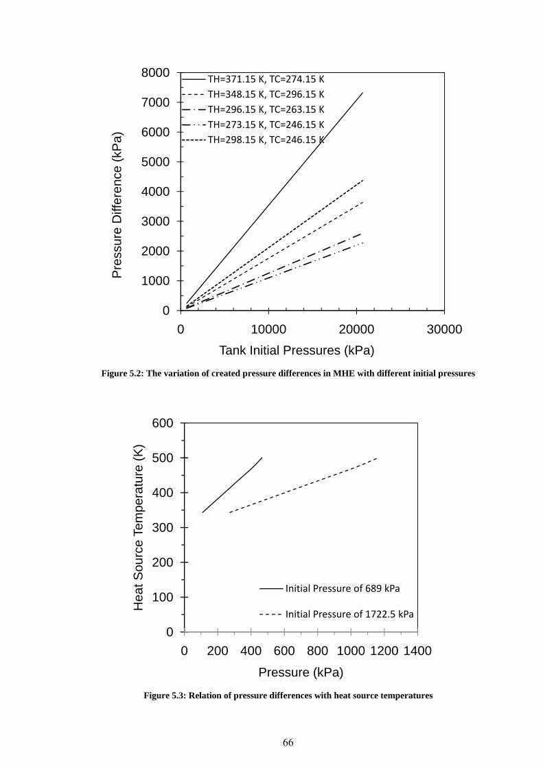
66
Figure 5.2: The variation of created pressure differences in MHE with different initial pressures
Figure 5.3: Relation of pressure differences with heat source temperatures
0
1000
2000
3000
4000
5000
6000
7000
8000
0 10000 20000 30000
Pre
ssur
e D
iffer
ence
(kP
a)
Tank Initial Pressures (kPa)
TH=371.15 K, TC=274.15 K
TH=348.15 K, TC=296.15 K
TH=296.15 K, TC=263.15 K
TH=273.15 K, TC=246.15 K
TH=298.15 K, TC=246.15 K
0
100
200
300
400
500
600
0 200 400 600 800 1000 1200 1400
Hea
t Sou
rce
Tem
pera
ture
(K
)
Pressure (kPa)
Initial Pressure of 689 kPa
Initial Pressure of 1722.5 kPa
67
5.2 Mechanical Efficiency of Transmission System
To find the transmission efficiency, the engine was operated and tested five times
[62]. In each test, the number of piston strokes and power output from the generator
was found. The actual torque produced from this piston assembly, for a 689.48 kPa
pressure differential, is 42 Nm [59]. From Equations (4.45) and (4.46), the power
output from the piston is calculated. The mechanical power outputs were compared
with the electric power outputs from the generator. With that data, the summation of
losses that occurred through the transmission system and generator was calculated.
The average efficiency of the system in these experiments was 40%.
Table 5.1: Transmission and generator efficiency
Peak Power
(W) Stokes Per Minute RPM Piston Power (W)
Mechanical Efficiency
Run 1 81 59 44.25 195 0.42 Run 2 92 61 45.75 201 0.46 Run 3 81 60 45 198 0.41 Run 4 63 58 43.5 191 0.33 Run 5 72 59 44.25 194 0.37 Average 77.8 59.4 44.55 195.8 0.4
Source: [62]
The efficiency found for the transmission system is more accurate for pressure
differentials that are closer to the pressure differential of the test (689.48 kPa). This is
because the speed of the flywheel is less at lower pressures. When higher pressure
differentials exist in the tanks, the flywheel speed is higher. Therefore, it is predicted
that for low pressure differentials, the efficiency of the system is higher than 40%, and
at higher pressure differentials, the efficiency is lower.
The fourth column of Table (5.1) shows the engine speed. It has an average of
44.55 RPM. The standard deviation of this column is 0.85. Considering this number,
the precision limit (P) is 0.04. The bias limit is estimated as half of the smallest scale

68
of the forth column which is 0.003. This precision limit and bias number result in a
3.85% uncertainty in the power calculations.
5.3 Efficiency of Mechanical Components in the MHE
To calculate the mechanical efficiency of the MHE, two major parts of the system
were considered. The first part was losses in the piston assembly sealing, and friction
between the rack and pinion of the piston cylinder assembly. The second portion of
losses occurs in the transmission system. From the manufacturer’s specifications, the
losses in the current assembly are in the range of 13-20% of energy output from the
pinion. In this study in order to consider losses due to pressure drops, a maximum of
20% was considered in calculation [59].
As mentioned in the section 5.2, the efficiency of the transmission in the
current system has an average of 40%. The piston assembly and transmission system
function in series, thus, when both are operating in series, the overall efficiency is
found by multiplying them. Hence, the overall mechanical efficiency of these two
systems is about 32%.
5.4 Pressure Measurements of MHE
In this section, experimental readings obtained from the pressure sensors are
presented. To achieve accurate results, the engine was operated several times. Some
observed results were not useful because of problems with the installation of pressure
tubes for sensors. Accurate readings were obtained from the first pair of tanks.
Figure 5.4 shows how the pressures vary in one pair of heat exchangers (hot
and cold) during the operating period. To perform this experiment, one tank was filled
with a pressure of 882.53 kPa, and the pressure of the other tank was 103.42 kPa.

69
Before starting the operation, there was a 160 second delay. Within this period, as
demonstrated in Figure 5.4, the pressure inside tank 1 dropped. This happened since
the temperature of the compressed air was higher than the ambient temperature
initially, and shells of the heat exchangers were not completely insulated. Thus, heat
transfer from the air to the shells, and from the shells to the surroundings, occurred. In
tank 2, the initial pressure inside the shell was close to the ambient pressure, hence
within the first 160 seconds, no considerable pressure change was observed in tank 2.
Figure 5.4: Pressure variations in one pair of heat exchangers during the operation period.
When the engine operation starts, due to heat and mass transfer from tank 1
into tank 2, the pressure of tank 1 decreases and the pressure of tank 2 increases
simultaneously. The curved sections in Figure 5.4 represent this period. When the
piston operation finished, the pressures inside the tanks did not equalize. The

70
remaining pressure difference was about 20.68 kPa in the experiment. The reason is
because of friction losses in the piston assembly, so the remaining pressure difference
could not move the piston.
5.5 Power Output Measurements from MHE
In this section, the measured power outputs from the piston assembly and generator
are presented. The desired pressure differences were simulated for the tests. Before
these tests, tanks were filled with compressed air at different pressures in each.
During the experiments, hot and cold water passed through the heat exchangers, in
order to heat up and cool them down. To find the power output from the heat engine,
the engine was run several times at the same pressure differential and ambient
conditions. Figure 5.5 shows the total power output from the electric generator during
one cycle. The horizontal axis in this figure shows the initial pressure difference
between the tanks. The separate points in this graph show the summation of power
outputs from the MHE under specific initial pressures. To obtain reasonable values
for each pressure differential, the engine was operated at least three times for each
initial pressure differential. The results shown in Figures 5.5 - 5.9 were the closest
results to the average readings of one set of experiments.
From the trend line in Figure 5.5, when the engine works under higher
pressure differences, the electricity generated from the system is increased.
Figure 5.6 shows the total mechanical power output from the piston assembly
at certain pressure differences. The mechanical power outputs are calculated by
measuring the number of piston revolutions, within a certain time period, and the
piston specifications from the manufacturer’s catalogue. The numbers of piston
revolutions were found by measuring the number of changes (open/close) of the
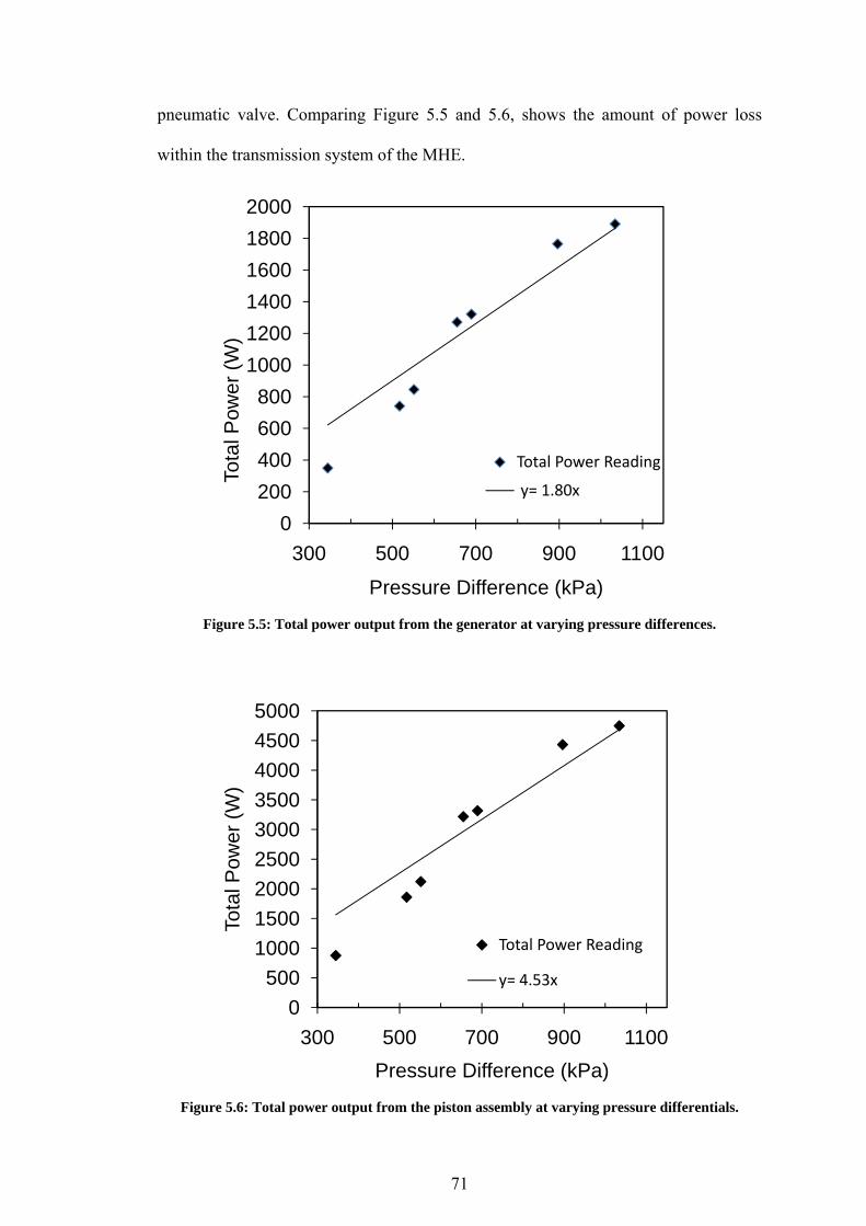
71
pneumatic valve. Comparing Figure 5.5 and 5.6, shows the amount of power loss
within the transmission system of the MHE.
Figure 5.5: Total power output from the generator at varying pressure differences.
Figure 5.6: Total power output from the piston assembly at varying pressure differentials.
0
200
400
600
800
1000
1200
1400
1600
1800
2000
300 500 700 900 1100
Tota
l Pow
er (
W)
Pressure Difference (kPa)
Total Power Reading
y= 1.80x
0
500
1000
1500
2000
2500
3000
3500
4000
4500
5000
300 500 700 900 1100
Tota
l Pow
er (
W)
Pressure Difference (kPa)
Total Power Reading
y= 4.53x
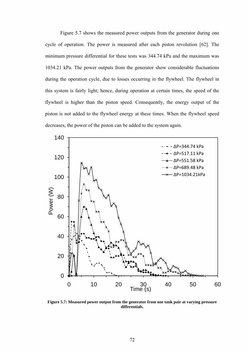
72
Figure 5.7 shows the measured power outputs from the generator during one
cycle of operation. The power is measured after each piston revolution [62]. The
minimum pressure differential for these tests was 344.74 kPa and the maximum was
1034.21 kPa. The power outputs from the generator show considerable fluctuations
during the operation cycle, due to losses occurring in the flywheel. The flywheel in
this system is fairly light; hence, during operation at certain times, the speed of the
flywheel is higher than the piston speed. Consequently, the energy output of the
piston is not added to the flywheel energy at these times. When the flywheel speed
decreases, the power of the piston can be added to the system again.
Figure 5.7: Measured power output from the generator from one tank pair at varying pressure differentials.
0
20
40
60
80
100
120
140
0 10 20 30 40 50 60
Pow
er (
W)
Time (s)
∆P=344.74 kPa
∆P=517.11 kPa
∆P=551.58 kPa
∆P=689.48 kPa
ΔP=1034.21kPa

73
In Figure 5.8, the points represent the measured power outputs from the
generator at two different pressure differentials. The continuous line shows the
predicted power output from the generator at an 779.11 kPa initial pressure
differential. The experimental pressure readings for this power prediction are
presented in Figure 5.4. At this specific pressure differential (779.11 kPa), no power
output reading was available from the generator. To validate the predicted power
output from the generator, the power output measurements from the upper and lower
pressure differentials were used. As expected, this line is located between the power
output readings of the initial pressure difference of 689.48 and 1034.48 kPa.
Figure 5.8: Comparison of measured and predicted power outputs from the generator for varying pressure differentials during one operation cycle.
The line that predicts the power output starts from a maximum value and
drops over time gradually. However, the practical power measurements start from
0
20
40
60
80
100
120
0 20 40 60
Pow
er O
utpu
t (W
)
Time (S)
Theory ( ΔP= 779.11 kPa)
Measured (ΔP= 1034.21 kPa)
Measured (ΔP= 689.48 kPa)

74
almost zero, go higher, drop drastically and the power reaches its maximum. The
reason for this trend is the initial energy required to rotate the flywheel. The first
stroke is so powerful that afterwards, for about 2 seconds, no power is added to the
flywheel. This trend is visible in almost all measured data from the MHE (Figure 5.7).
Figures (5.7) and (5.8) show that the power output from the generator in the current
prototype is not uniform. Sections (5.7.2) and (5.7.3) show the configurations of the
MHE that can generate steady power output.
Figure 5.9 shows a comparison of measured and predicted peak power outputs
from the generator for varying pressure differentials. Seven observed peak power
outputs at certain initial pressures are shown in this graph. The continuous solid line
shows the predicted peak power outputs from the generator. The closest match
between the model and observed data occurs between the initial pressures of 600 and
700 kPa. At pressures around 1000 kPa, the model predicts higher power outputs from
the system than the observed numbers. This is because the transmission efficiency
was measured at 689.48 kPa. At higher pressure differentials, the rotary speed of the
flywheel increases. Thus, more energy from the piston revolutions cannot be captured.
Therefore, at high pressure differentials, the mechanical efficiency of the transmission
system is less than 40%.
5.6 System Efficiency
The Carnot efficiency of the heat engines was discussed in chapter four. Figure 5.10
shows the Carnot efficiency of the system. The temperature ranges for the heat source
and the heat sink in this study are between 272.15 K to 372.15 K. Practical
applications; typically reside within this temperature range. In addition, in many areas
of industry, waste heat in this temperature range is freely available. If solar source is
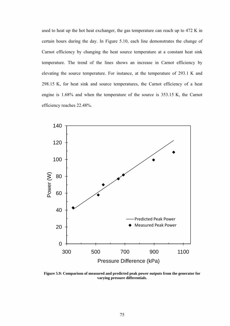
75
used to heat up the hot heat exchanger, the gas temperature can reach up to 472 K in
certain hours during the day. In Figure 5.10, each line demonstrates the change of
Carnot efficiency by changing the heat source temperature at a constant heat sink
temperature. The trend of the lines shows an increase in Carnot efficiency by
elevating the source temperature. For instance, at the temperature of 293.1 K and
298.15 K, for heat sink and source temperatures, the Carnot efficiency of a heat
engine is 1.68% and when the temperature of the source is 353.15 K, the Carnot
efficiency reaches 22.48%.
Figure 5.9: Comparison of measured and predicted peak power outputs from the generator for varying pressure differentials.
0
20
40
60
80
100
120
140
300 500 700 900 1100
Pow
er (
W)
Pressure Difference (kPa)
Predicted Peak Power
Measured Peak Power

76
Figure 5.12 shows the variation of Carnot efficiency for certain temperature
differentials. From this figure, having the same temperature differences in lower
temperature ranges gives higher Carnot efficiencies of the heat engine. When the heat
sink temperature is 273.15 K, the efficiency of the heat engine is higher than 283.15 K
and 293.l5 K. This trend is valid for temperature differentials below zero as well. Also
in Figure 5.9, the maximum possible efficiency achievable from this system in
temperature ranges of 273.15 K to 373.15 K is 27.77%. Consequently, when water is
used to bring and remove heat from the system, the thermal efficiency of the system
cannot exceed 27.77%.
Figure 5.10: Variations of Carnot efficiency at different source temperatures.
0
5
10
15
20
25
30
270 295 320 345 370
Car
not E
ffici
ency
(%
)
TH (K)
Tc=283.15 K
Tc=293.15 K
Tc=273.15 K

77
Figure 5.11: Variations of Carnot efficiency with different temperature ranges.
Figure 5.12 shows the energy and exergy efficiency of the system at varying
pressure differentials. In this figure, the heat source and heat sink temperatures are
298.15 K and 342.15 K, respectively. The results are based on models and
experimental mechanical efficiency of the system. From Figure 5.11, at higher initial
pressures, the energy and exergy efficiencies of the system increase. Exergy and
energy efficiency of the MHE with the heat sink and source temperatures of 273.15 K
and 289.15oK, are presented in Figure 5.11. When the air mass inside the tanks
increases, the amount of heat that is transferred from the water stream to the air will
raise. Therefore Increasing initial pressure of the MHE raises the energy and exergy
efficiencies of the system Comparing Figures 5.12 and 5.13 clearly demonstrates that
the effect of the temperature differential of the heat source and sink on the MHE is
0
2
4
6
8
10
12
14
16
0 50 100
Car
not E
ffici
ency
(%
)
TC (K)
Δ T=15 K
Δ T=45 K
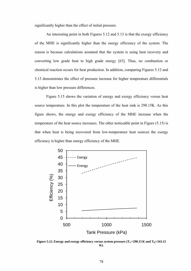
78
significantly higher than the effect of initial pressure.
An interesting point in both Figures 5.12 and 5.13 is that the exergy efficiency
of the MHE is significantly higher than the energy efficiency of the system. The
reason is because calculations assumed that the system is using heat recovery and
converting low grade heat to high grade energy [63]. Thus, no combustion or
chemical reaction occurs for heat production. In addition, comparing Figures 5.12 and
5.13 demonstrates the effect of pressure increase for higher temperature differentials
is higher than low pressure differences.
Figure 5.15 shows the variation of energy and exergy efficiency versus heat
source temperature. In this plot the temperature of the heat sink is 298.15K. As this
figure shows, the energy and exergy efficiency of the MHE increase when the
temperature of the heat source increases. The other noticeable point in Figure (5.15) is
that when heat is being recovered from low-temperature heat sources the exergy
efficiency is higher than energy efficiency of the MHE.
Figure 5.12: Energy and exergy efficiency versus system pressure (TC=298.15 K and TH=343.15
K).
0
5
10
15
20
25
30
35
40
45
50
500 1000 1500
Effi
cien
cy (
%)
Tank Pressure (kPa)
Exergy
Energy
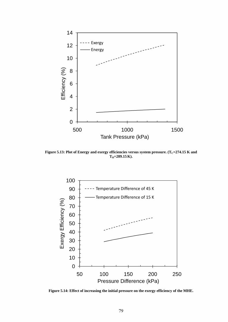
79
Figure 5.13: Plot of Energy and exergy efficiencies versus system pressure. (TC=274.15 K and TH=289.15 K).
Figure 5.14: Effect of increasing the initial pressure on the exergy efficiency of the MHE.
0
2
4
6
8
10
12
14
500 1000 1500
Effi
cien
cy (
%)
Tank Pressure (kPa)
Exergy
Energy
0
10
20
30
40
50
60
70
80
90
100
50 100 150 200 250
Exe
rgy
Effi
cien
cy (
%)
Pressure Difference (kPa)
Temperature Difference of 45 K
Temperature Difference of 15 K

80
Figure 5.15: Effect of increasing the heat source temperature on the energy and exergy efficiency of the MHE.
5.7.1 Possible Improvements of the Current System
In the current system, two pairs of heat exchangers are used to create pressure
differences. As shown in Chapter Five, the efficiency of the transmission system is
about 40%. This efficiency can be increased by altering some parts. Figure 6.1 shows
a schematic of the transmission system in the current MHE.
In this system, a poly V type belt is connecting the flywheel to the electricity
generator. The pulley for the generator was grooved; however, the flywheel had no
groove on the edge. Due to the speed variations of the flywheel, the connecting belt
slips on the pulley while it drives the generator. These slippery movements will result
in kinetic energy losses.
0
10
20
30
40
50
60
250 300 350 400
Effi
cien
cy (
%)
TH (K)
Energy
Exergy
81
Furthermore, when the belt is tightening strongly, the force on the bearings
increases and the rate of friction losses will be higher. When the belt is not tight
enough, the pulley slippage will increase. To overcome this problem, the tightness of
the belt has to be checked frequently, to maintain good performance of the heat
engine.
A possible substitute for the poly V type belt is a toothed belt, a toothed
pulley, and a flywheel. In this case, the down time of the machine will be reduced,
and the amount of energy lost as a result of slip will decrease. Another way to reduce
the losses and the maintenance cost is by changing the belt with a chain. There are
two potential disadvantages that may occur with this replacement.
1. The chain transmission is noisier than the belt system.
2. The life of the shaft keys will be reduced due to sudden speed changes of
the pulley.
In the current system, the diameter of the flywheel is 36cm and the diameter of
the connected pulley to the generator is 5 cm. The speed of the pulley generator is
about seven times more than the flywheel speed, and the diameter of the generator
pulley is too small compared with the flywheel. Therefore, to avoid a sudden speed
change, the speed change can be done in two steps. This rapid speed change can be
improved by using another pulley, which has a ratio between the current generator
pulley ratio and the flywheel ratio.
5.7.2 Possible Designs for the Next Marnoch Heat Engine
Prototype
In the previous section, possible improvements of the current system were discussed.
The proposed changes in section 5.7.1 required no major cost. In this section, three
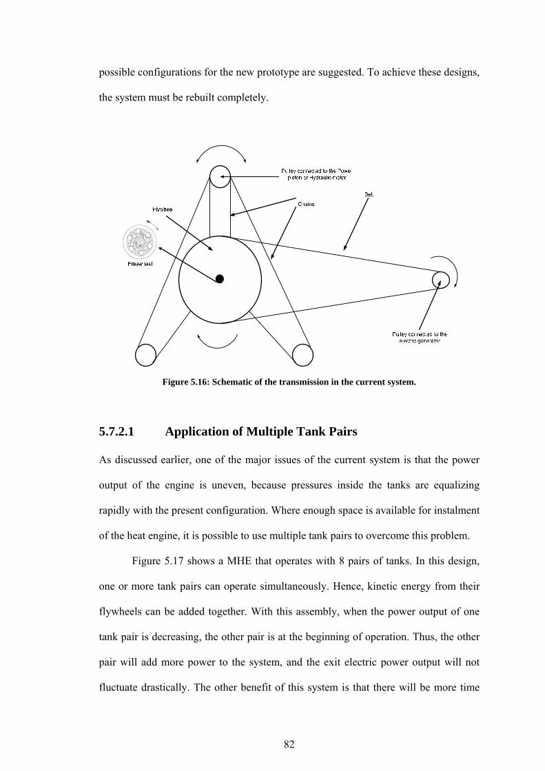
82
possible configurations for the new prototype are suggested. To achieve these designs,
the system must be rebuilt completely.
Figure 5.16: Schematic of the transmission in the current system.
5.7.2.1 Application of Multiple Tank Pairs
As discussed earlier, one of the major issues of the current system is that the power
output of the engine is uneven, because pressures inside the tanks are equalizing
rapidly with the present configuration. Where enough space is available for instalment
of the heat engine, it is possible to use multiple tank pairs to overcome this problem.
Figure 5.17 shows a MHE that operates with 8 pairs of tanks. In this design,
one or more tank pairs can operate simultaneously. Hence, kinetic energy from their
flywheels can be added together. With this assembly, when the power output of one
tank pair is decreasing, the other pair is at the beginning of operation. Thus, the other
pair will add more power to the system, and the exit electric power output will not
fluctuate drastically. The other benefit of this system is that there will be more time

83
vacant for each tank pair to be charged. Figure 5.18 shows the trend of the possible
power output of a MHE with two and multiple pairs of tanks.
The lines in Figure 5.18 show the trend of power output from the generator.
Lines in Figure 5.18a are not connected to each other and they have dramatic ups and
downs with time. The gaps between vertical lines in that graph represent the time gaps
where no power is generated by the heat engine. This time gap exists because of the
required time for switching the tank pairs. If the valves that switch the tanks can
operate faster, this gap will be reduced and more power will be generated by the
MHE.
In Figure 5.18b, the line, which shows the power output, is a continuous line
and has minor fluctuations in comparison to Figure 5.18a. The curved lines at the
bottom of Figure 5.18b represent the power generated by each pair of tank. The
overall electric power output in this graph is located at the top of the graph
(represented by a continuous line). It is the summation of individual curves. In the
next section, effects of using one generator for all heat exchangers and separated
generators for each tank pair, in a multiple tank pair configuration will be discussed.
5.7.2.1.1 MHE with Multiple Pairs of Tanks and One Electric
Generator
When the MHE operates with multiple pairs of tanks, more than one pair of
heat exchangers are operating at the same time, and the torque output from their
pistons does not have the same value. This occurs because some are at the beginning
of their operation period, and the others are in the last steps of the discharging mode.
When the piston energy output is converted to rotary kinetic energy in the flywheel,
the angular speed of each flywheel is different. Freewheels can be used to connect
each pulley to the shaft. In this way, when the speed of one flywheel reduces, it does

84
not break the momentum of the other flywheels.
COLD
COLD
HOT
HOT
COLD
COLDHOT
HOT
HOTCOLD
HOTCOLD
HOTCOLD
COLD HOT
Flywheel
Crank shaft
Piston- Cylinder Assembly
Pressurized Tanks
Figure 5.17: MHE with 8 tank pairs.
In this configuration, when the speeds of the individual pulleys are less than
the main flywheel speed, no energy is added from that tank pair to the main shaft. In
this case, it can be observed that pistons are acting and the connected flywheels are
rotating. Nevertheless, no energy is being transferred through the shaft to the
flywheel. The weight of the main flywheel, which is connected to the generator, must
be optimized in the way that the maximum possible energy from each tank pair is
captured.
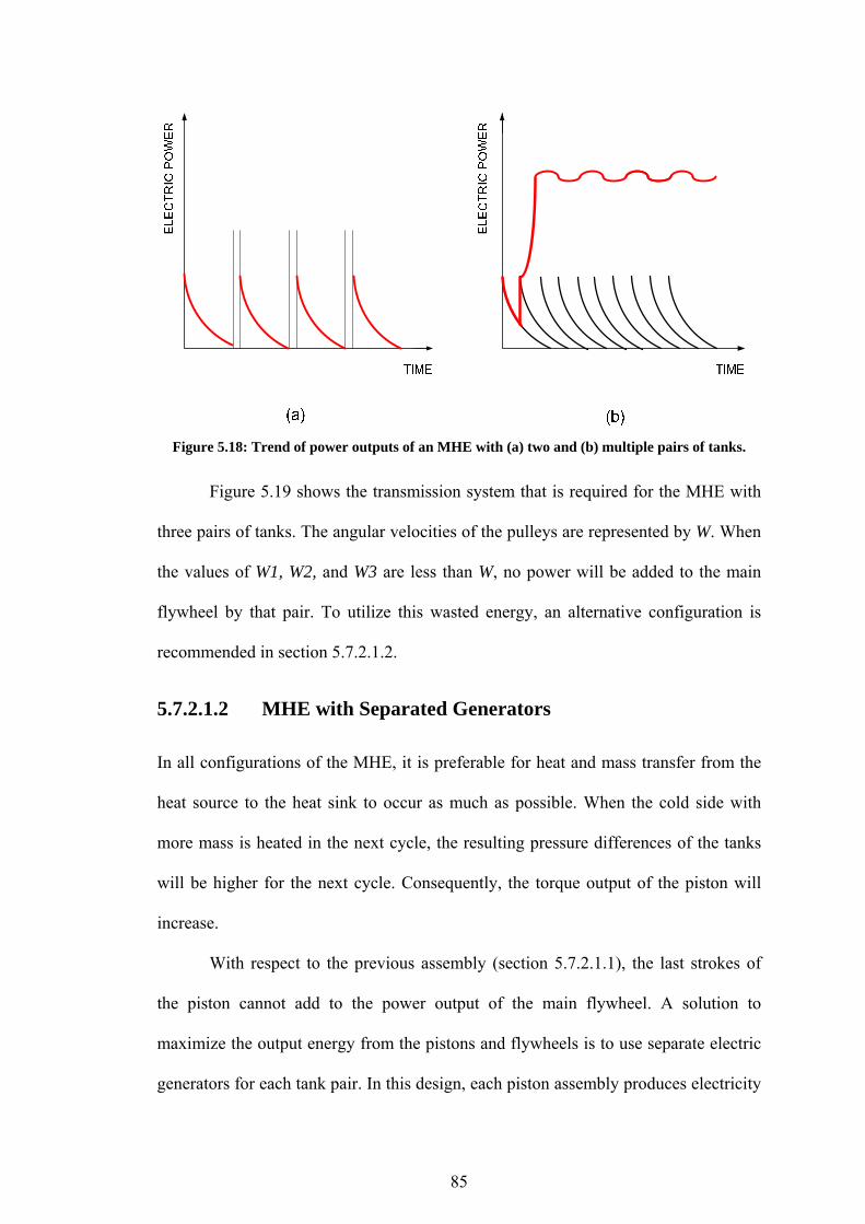
85
Figure 5.18: Trend of power outputs of an MHE with (a) two and (b) multiple pairs of tanks.
Figure 5.19 shows the transmission system that is required for the MHE with
three pairs of tanks. The angular velocities of the pulleys are represented by W. When
the values of W1, W2, and W3 are less than W, no power will be added to the main
flywheel by that pair. To utilize this wasted energy, an alternative configuration is
recommended in section 5.7.2.1.2.
5.7.2.1.2 MHE with Separated Generators
In all configurations of the MHE, it is preferable for heat and mass transfer from the
heat source to the heat sink to occur as much as possible. When the cold side with
more mass is heated in the next cycle, the resulting pressure differences of the tanks
will be higher for the next cycle. Consequently, the torque output of the piston will
increase.
With respect to the previous assembly (section 5.7.2.1.1), the last strokes of
the piston cannot add to the power output of the main flywheel. A solution to
maximize the output energy from the pistons and flywheels is to use separate electric
generators for each tank pair. In this design, each piston assembly produces electricity

86
until the last revolution of the piston. Figure 5.20 shows a schematic of this design. In
this figure, only the major transmission components of the assembly are shown.
Figure 5.19: Required transmission system for three pairs of tanks.
In addition to energy loss reduction, the other advantage of this system is that
the mass of the flywheels can have more variations in comparison to the design
specifications in section 5.7.2.1.1. One disadvantage of this design is that due to
separate generators, the capital cost of the unit and the maintenance costs are high.
The other issue is space limitation, as this system requires larger space for installation.
5.7.3 Marnoch Heat Engine with Hydraulic Motors
In the current MHE, a pneumatic piston is used to produce power from pressure
differentials. Another alternative that can be used to convert pressure differentials to
mechanical shaft work is a hydraulic system. In this configuration, two external heat
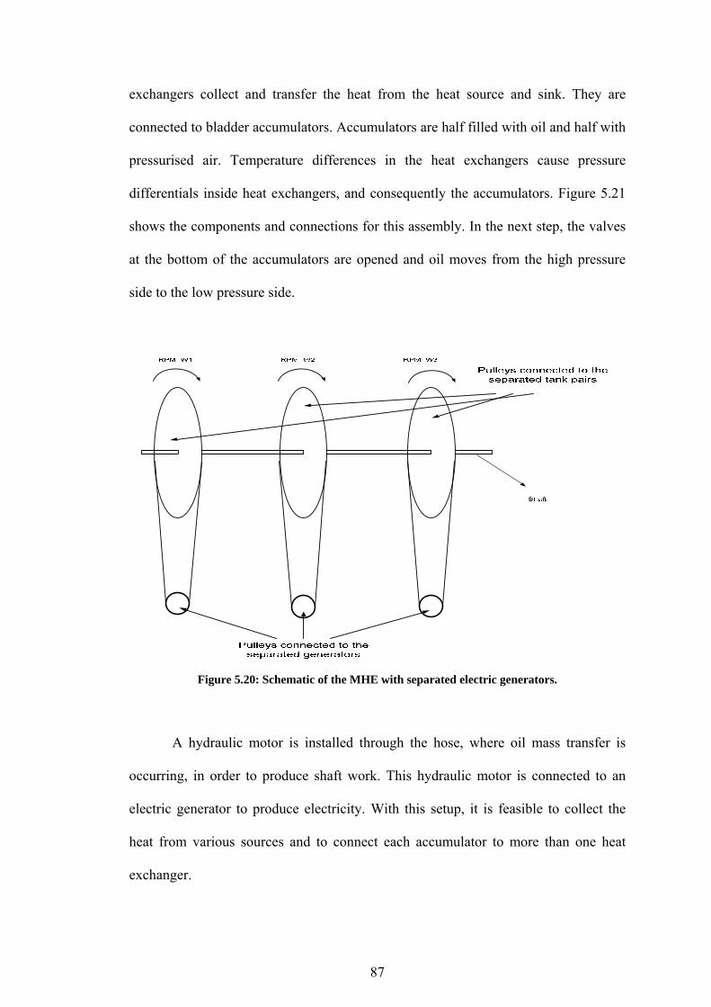
87
exchangers collect and transfer the heat from the heat source and sink. They are
connected to bladder accumulators. Accumulators are half filled with oil and half with
pressurised air. Temperature differences in the heat exchangers cause pressure
differentials inside heat exchangers, and consequently the accumulators. Figure 5.21
shows the components and connections for this assembly. In the next step, the valves
at the bottom of the accumulators are opened and oil moves from the high pressure
side to the low pressure side.
Figure 5.20: Schematic of the MHE with separated electric generators.
A hydraulic motor is installed through the hose, where oil mass transfer is
occurring, in order to produce shaft work. This hydraulic motor is connected to an
electric generator to produce electricity. With this setup, it is feasible to collect the
heat from various sources and to connect each accumulator to more than one heat
exchanger.

88
Figure 5.21: MHE with external heat exchangers and hydraulic motor.
In the other alternative setup, heat transfer occurs in the gas section of the heat
exchangers. By the application of the internal heat exchangers, the occupied area of
the MHE will decrease in comparison to the configuration with external heat
exchangers. Thus, for highly compact pressure units, this configuration can be
considered.
The advantages of using a hydraulic system in the MHE, in comparison to the
pneumatic system, are listed below:
The noise produced by a hydraulic system is significantly less than a
pneumatic system.
Power consumption by the valves is less than the pneumatic system.
Durability and operation of valves are better in the hydraulic system.
It gives a smaller hydraulic system for the same power output.
Maintaining isothermal expansions and compressions are easier in a hydraulic
system, since there is no fast change of mass transfer direction.
89
The MHE with a hydraulic system works smoother than an MHE with a
pneumatic system. Therefore, it is expected to obtain power output from this
system with fewer power fluctuations (Figure 5.23).
Figure 5.23a shows a possible trend of power outputs from the MHE with two
pairs of tanks and a hydraulic system. Figure 5.23b depicts the power generation from
the MHE with multiple heat exchangers and a hydraulic system.
A preliminary assembly was established in order to observe and study the
performance of the hydraulic systems. Figure 5.24 shows an image of the current
setup. The maximum pressure that can be used in these bladder accumulators is
20,684 kPa. In the present setup, accumulators were filled with air at 1,034 kPa, since
the external heat exchangers were not certified to hold more than 1,034 kPa. The
accumulators were filled with five litres of oil. In the current setup, all ball valves
were manually operated.
When operation of the system started, the hydraulic motor was rotating
smoothly until the existing pressure differential was not able to run the motor. The
challenge of this system is friction inside the hydraulic motor. When the pressure
difference between tanks was about 68 kPa, the system stopped working. Thus, for
further applications, the components of the motor must be altered to reduce the motor
friction.
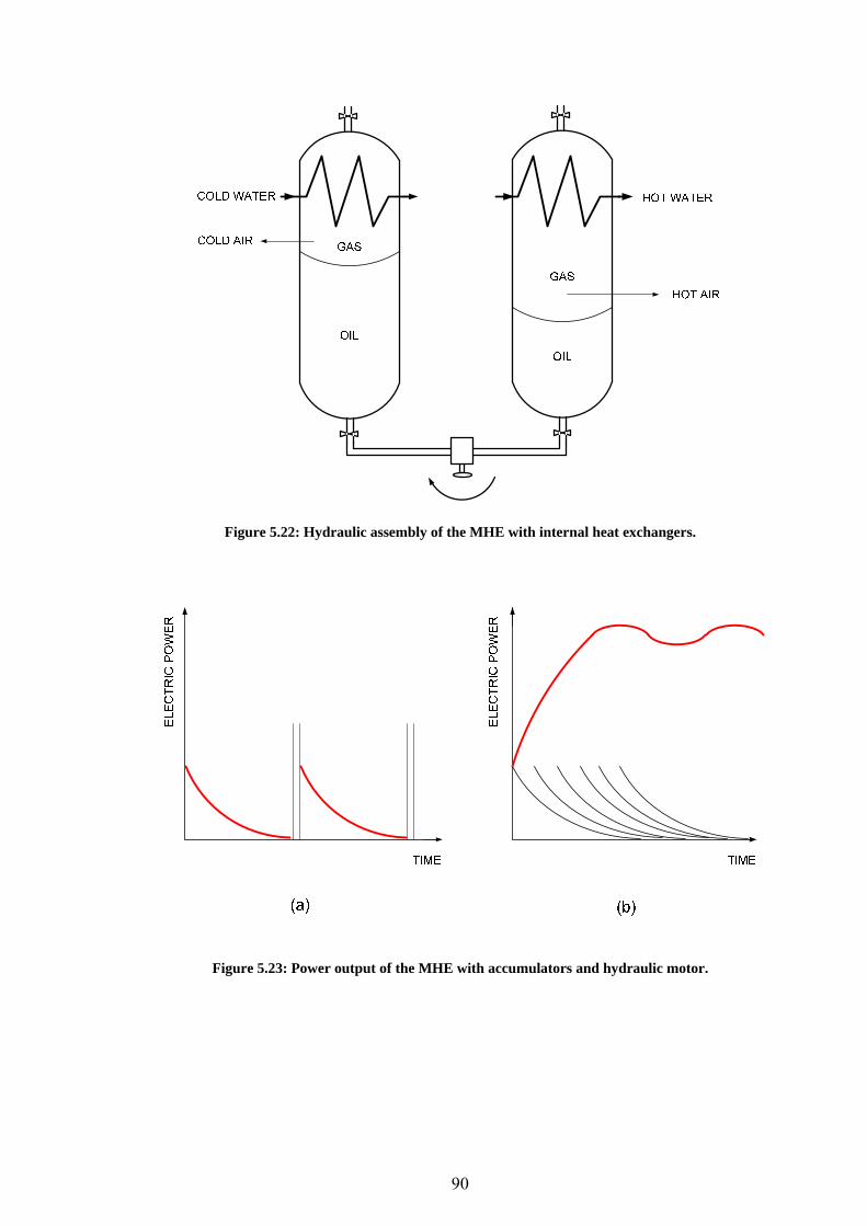
90
Figure 5.22: Hydraulic assembly of the MHE with internal heat exchangers.
Figure 5.23: Power output of the MHE with accumulators and hydraulic motor.
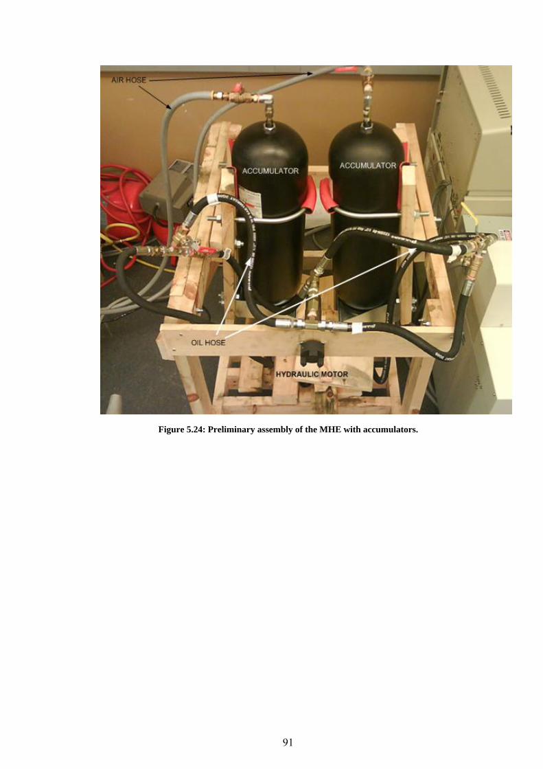
91
Figure 5.24: Preliminary assembly of the MHE with accumulators.

92
Chapter 6:
Conclusions and Recommendations for Future
Research
6.1 Conclusions
The Marnoch heat engine is an energy conversion device that has the capability to
convert low grade heat to electricity. As described in this thesis, MHEs have good
potential for being used in many applications. Its commercialization for stationary
applications is promising. The engine can utilize waste heat from nuclear, fossil fuel
or renewable fuelled power plants. The main conclusions of this thesis are listed
below:
• The engine can operate continually when a suitable heat source and heat sink
are available;
• Having higher temperature differentials increases the power output from the
MHE;
• For a higher initial pressure in the heat exchangers, there is higher power
output; and
• The Marnoch heat engine is commercially viable.
6.2 Recommendations for Future Research
A thorough design optimization is recommended for the system, using computing
facilities, to find the optimum parameters such that the best system performance. It is

93
also recommended to build a flexible prototype to study the system in practice, and
validate the theoretical studies in another way as well.
Potential modifications were presented in section 5.7. The following list shows
suggested studies to be performed to achieve better performance from the MHE.
Moreover, some recommended modifications for the components are also listed
below:
Increasing the piston-cylinder volume when the piston is used for energy
conversion;
Optimizing the flywheel weight for each piston assembly and pressure
differential;
Perform a detailed study on the hydraulic motors for energy conversion;
Study of different accumulators;
Finding faster valves using less energy;
Use of better hoses and joints to decrease the pressure drops as much as
possible;
Use of higher ratio elbows to decrease the friction losses;
Replacing air with other working fluids which have higher heat transfer
coefficients;
Perform tests with low-temperature differentials to test the performance of the
engine;
Performing a detailed thermo-economic analysis of the MHE.

94
References
1. Dincer, I., "Renewable energy and sustainable development: a crucial review", Renewable and Sustainable Energy Reviews, Vol. 4, pp. 157-175, 2000.
2. Dincer, I., Rosen M. A., “Thermodynamic aspects of renewables and sustainable development”, Renewable and Sustainable Energy Reviews, Vol. 9, pp. 169-189, 2005.
3. Rasthal, J. E., Drennen,T. E., Pathways to a Hydrogen Future, 1st ed., UK: Elsevier, 2007.
4. Etcheverry, J., “Comments Regarding the Ontario Power Authority’s (OPA)”, Supply Mix Advice Report, David Suzuki Foundation, Toronto, February 2006.
5. EIA, “Emissions of Greenhouse Gases”, Report by the Energy Information Administration (EIA), US Department of Energy, “http://www.eia.doe.gov/”, August 22, 2008.
6. Rahm, D., Sustainable Energy and the States, Essay on Politics Markets and Leadership, 1st ed., North Carolina: McFarland, 2002.
7. Anon, A., "World Energy Council, Technical Report", Global energy perspectives to 2050 and beyond, London, 1995.
8. Randolf, J., Masters, G. M., Energy for Sustainability, 1st ed.,Washington: Island Press, 2008.
9. Tester, J. W., Drake, E. M., Golay, M. W., Peters, W. A., Sustainable Energy Choosing Among Options, 1st ed., Massachusetts: MIT Press, 2005.
10.”http://www.dauphine.fr/cgemp/Publications/Articles/PAPER%20MOSCOW%20CPZ.pdf”, Contribution of coal and nuclear to sustainable energy, supply: perspectives and problems, Dauphine University of Paris, Paper presented at the Russian Academy of Sciences, Academies of Sciences, President’s meeting of G8 countries, Brazil, China, India and South Africa, Moscow, April 2006.
11. Caldicott, H., Nuclear Power is Not the Answer to Global Warming or Anything Else, 1st ed., New York: The New Press, 2006.
12. Turner, W. C., Energy Management Handbook, 5th ed., Washington: The Fairmont Press, 2005.
13. OECD, “http://www.oecd.org/document/”, Report by the Organization for Economic Co-opration and Development, Economic, Environmental and Social Statistics, May 12, 2009.
14. Spiro, T. G., Stigliani, W. M., Environmental Issues in Chemical Perspective, 1st ed., New York: State University of New York Press ,1980.

95
15. Beer, J. M., “High efficiency electric power generation, The environmental role”, Progress in Energy and Combustion Science, Vol. 33, pp. 107–134, 2007.
16. Ehrlich, K., Konys, J., Heikinheimo, L., “Materials for high performance light water reactors”, Journal of Nuclear Materials, Vol. 327, pp. 140–147, 2004.
17. Viswanathan, R., Henry, J. F., Tanzosh, J., Stanko, G., Shingledecker, J., Vitalis, B., Purgert, R, “U.S. program on materials technology for ultra-supercritical coal power Plants”, ASM International, Vol. 14, pp. 281-292, 2005.
18. “http://www.berr.gov.uk/files/file30703.pdf”, Brochure, Advanced Power Plant Using High Efficiency Boiler/Turbine, September 25, 2006.
19. Hardel, J., Kassfeldt, E., Prakash, B., “Friction and wear behaviour of high strength boron steel at elevated temperatures of up to 800 oC”, Wear, Vol. 264, pp. 788–799, 2007.
20. Zamrik, S. Y., Renauld, M. L., “Thermo-mechanical out-of-phase fatigue life of overlay coated IN-738LC gas turbine material”, Thermo-mechanical Fatigue Behavior of Materials, Vol. 3, pp. 119-137, 2000.
21. Tan, L., Ren, X., Sridharan, K., Allen, T. R., “Corrosion behavior of Ni-base alloys for advanced high temperature water-cooled nuclear plants”, Corrosion Science, Vol. 50, pp. 3056–3062, 2008.
22. Was, G. S., Ampornrat, P., Gupta, G., Teysseyre, S., West, E. A., Allen, T. R., Sridharan, K., Tan, L., Chen, Y., Ren, X., Pister, C., “Corrosion and stress corrosion cracking in supercritical water”, Journal of Nuclear Materials, Vol. 371, pp. 176–201, 2007.
23. Brown, L. F., “A comparative study of fuels for on-board hydrogen production for fuel-cell-powered automobiles”, International Journal of Hydrogen Energy, Vol. 26, pp. 381–397, 2001.
24. Nojoumi, H., Dincer, I., Naterer, G. F., “Greenhouse gas emissions assessment of hydrogen and kerosene-fueled aircraft propulsion”, International Journal of Hydrogen Energy, Vol. 34, pp. 1363-1369, 2009.
25. Sesto, E., Casale, C., “Exploitation of wind as an energy source to meet the world's electricity demand”, Journal of Wind Engineering and Industrial Aerodynamics, Vol. 74, pp. 375-387, 1998.
26. Cassedy, E. S., Prospects for sustainable energy: a critical assessment, 1st ed., Cambridg: University Press, 2000.
27. Maegaard, P., Bassam, N., Integrated Renewable Energy for Rural Communities: Planning Guidelines, Technologies and Applications, 1st ed., UK: Elsevier Science, 2004.
28. Nojoumi, H., “Investigation of a New Bipolar Design for PEM Fuel Cells”, Thesis (MASc), Faculty of Engineering and Applied Science, University of Ontario Institute of Technology, Oshawa, Canada, July 2009.
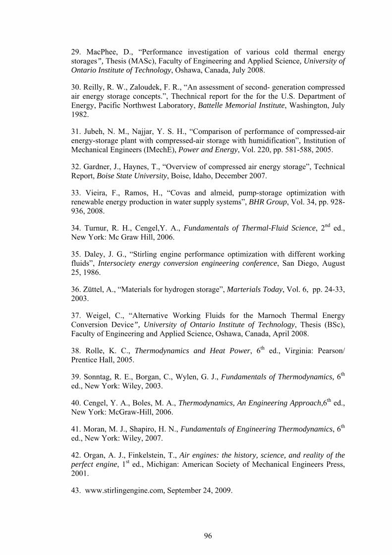
96
29. MacPhee, D., “Performance investigation of various cold thermal energy storages”, Thesis (MASc), Faculty of Engineering and Applied Science, University of Ontario Institute of Technology, Oshawa, Canada, July 2008.
30. Reilly, R. W., Zaloudek, F. R., “An assessment of second- generation compressed air energy storage concepts.”, Thechnical report for the for the U.S. Department of Energy, Pacific Northwest Laboratory, Battelle Memorial Institute, Washington, July 1982.
31. Jubeh, N. M., Najjar, Y. S. H., “Comparison of performance of compressed-air energy-storage plant with compressed-air storage with humidification”, Institution of Mechanical Engineers (IMechE), Power and Energy, Vol. 220, pp. 581-588, 2005.
32. Gardner, J., Haynes, T., “Overview of compressed air energy storage”, Technical Report, Boise State University, Boise, Idaho, December 2007.
33. Vieira, F., Ramos, H., “Covas and almeid, pump-storage optimization with renewable energy production in water supply systems”, BHR Group, Vol. 34, pp. 928-936, 2008.
34. Turnur, R. H., Cengel,Y. A., Fundamentals of Thermal-Fluid Science, 2nd ed., New York: Mc Graw Hill, 2006.
35. Daley, J. G., “Stirling engine performance optimization with different working fluids”, Intersociety energy conversion engineering conference, San Diego, August 25, 1986.
36. Züttel, A., “Materials for hydrogen storage”, Marterials Today, Vol. 6, pp. 24-33, 2003.
37. Weigel, C., “Alternative Working Fluids for the Marnoch Thermal Energy Conversion Device”, University of Ontario Institute of Technology, Thesis (BSc), Faculty of Engineering and Applied Science, Oshawa, Canada, April 2008.
38. Rolle, K. C., Thermodynamics and Heat Power, 6th ed., Virginia: Pearson/ Prentice Hall, 2005.
39. Sonntag, R. E., Borgan, C., Wylen, G. J., Fundamentals of Thermodynamics, 6th ed., New York: Wiley, 2003.
40. Cengel, Y. A., Boles, M. A., Thermodynamics, An Engineering Approach,6th ed., New York: McGraw-Hill, 2006.
41. Moran, M. J., Shapiro, H. N., Fundamentals of Engineering Thermodynamics, 6th ed., New York: Wiley, 2007.
42. Organ, A. J., Finkelstein, T., Air engines: the history, science, and reality of the perfect engine, 1st ed., Michigan: American Society of Mechanical Engineers Press, 2001.
43. www.stirlingengine.com, September 24, 2009.

97
44. ”http://wood-pellet-ireland.blogspot.com/”, Stirling Engine Reference, Guide and Catalog, September 24, 2009.
45. Kongtragool, B., Wongwises, S., “A review of solar-powered Stirling engines and low temperature differential Stirling engines”, Renewable and Sustainable Energy Reviews, Vol. 7, pp. 131–154, 2003.
46. Andersen, Kildegard, S., “Numerical Simulation of Cyclic Thermodynamic Processes”, Thesis (Ph.D), Department of Mechanical Engineering, Energy Engineering, Technical University of Denmark, Lyngby, Copenhagen, March 2006.
47. Berchowitz, D. M., Shonder, J., “Estimated size and performance of a natural gas fired duplex stirling for domestic refrigiration applications”, Technical report, Oak Ridge National Labs, Oak Ridge, Tennessee, U. S. A, October 2008.
48. Karabulut, H., Aksoy, F., Ozturk, E., “Thermodynamic analysis of a Betta type Stirling engine with a displacer driving mechanism by means of a lever”, Renewable Energy, Vol. 34, pp. 202-208, 2009.
49. Eid, E., “Performance of a beta-configuration heat engine having a regenerative displacer”, Renewable Energy, Vol. 34, pp. 2404-2413, 2009.
50. Parlak, N., Wager, A., Elsener, M., Soyan, H. S., “Thermodynamid analysis of a gmma type stirling engine in non-ideal adiabatic conditions”, Renewable Energy, Vol. 34, pp. 266-273, 2009.
51. Abdullah, S., Yousif, B. F., Sopian, K., “Design consideration of lowtemperature differential double-acting Stirling engine for solar application”, Renewable Energy, pp. 1923–1941, 2005.
52. Kongtragool, B., Wongwieses, S., “A four power-piston low-temparature differential Stirling engine using simulated solar energy as heat source”, Solar Energy, 2008, Vol. 82, pp. 493-500.
53. Senft, J. R., Mechanical Efficiency of Heat Engines., 1st ed., New York: Cambridge University Press, 2007.
54. Marnoch, I., Naterer, G., Rosen, M. A., Weston, J., “Marnoch engine Performance for multiple pressure vessel configurations”, International Conference on Efficiency, Cost, Optimization, Simulation and Environmental Impact of Energy Systems, Istanbul, July 2008.
55. Chukwu, C. C., Naterer, G. F., Rosen, M. A., Dahlquist, E, Marnoch, I. A., “Thermal optimization and economic analysis of a Marnoch heat engine” Swedish National Energy Convention, Toronto, March 12-13, 2008.
56.“http://www.potashcorp.com/media/pdf/about/brochure/PCS_Mini_Mine_Tour_brochure.pdf”, Down Under, A mini tour, May 14, 2009.
57. Marnoch, I. A., Thermal conversion device and process, Patent Number 4389858, Canada, Jun 5, 2008.

98
58. Munson, B. R., Young, B. J., Okishi,T. H., Fundamentals of Fluid Mechanics,5th ed., New York: Wiley, 2005.
59. Pneumatic Automation Products, Manufacturer Catalogue, USA: Parker Hannifan Corporation, 2001.
60. Dincer, I., Rosen. M.A., Exergy: Energy, Environment and Sustainable Development , 1st ed., Elsevier, 2007.
61. Armstrong, A., Haseen, F., Marnoch, I., Weston, J., Naterer, G. F., Lu, L., Rosen, M. A. “Thermodynamic Design and Control of a Marnoch Thermal Energy Conversion Device”, Proceedings of 21st Canadian Congress of Applied Mechanics, Toronto, Canada, pp. 284-285, June 2007.
62. Self, S., “Power Testing of the Prototypical Marnoch Thermal Energy Conversion Device”, Thesis (BSc), Faculty of Engineering and Applied Science, University of Ontario Institue of Technology, Oshawa, Canada, April 2008.
63. Naterer, G. F., “Second law viability of upgrading waste heat for thermochemical hydrogen production”, International Journal of Hydrogen Energy, Vol. 33, pp. 6037-6045, 2008.