Thermocapillary migration of interfacial droplets

Thermocapillary migration of interfacial dropletsEdwin F. Greco and Roman O. GrigorievCenter for Nonlinear Science and School of Physics, Georgia Institute of Technology,Atlanta, Georgia 30332-0430, USA

�Received 31 August 2008; accepted 2 February 2009; published online 16 April 2009�

We study the thermocapillary driven motion of a droplet suspended at an interface of two fluidlayers subjected to an imposed temperature gradient parallel to the interface. We compute thetemperature and velocity fields inside and outside of the droplet using a boundary collocationnumerical scheme in the limit of small capillary and thermal Péclet numbers and compare the resultswith the classical problem of thermocapillary migration of a droplet in the bulk. In particular, wefind that, for typical values of parameters, interfacial droplets migrate in the direction opposite to thetemperature gradient, while in the classical problem migration is always in the direction of thegradient. Furthermore, we find that a rich variety of flow structures can emerge inside interfacialdroplets. We also confirm that for parameters matching a recent experimental study of mixing insideinterfacial microdroplets �R. O. Grigoriev, V. Sharma, and M. F. Schatz, Lab Chip 6, 1369 �2006��the interior flow can be approximated with reasonable accuracy by assuming the droplet to becompletely submerged in the bottom layer. © 2009 American Institute of Physics.�DOI: 10.1063/1.3112777�

I. INTRODUCTION

The first published investigation of thermocapillary mi-gration dates back almost 50 years to the work by Younget al.,1 who observed and analyzed the motion of air bubblesin silicon oil in response to the imposed temperature gradi-ent. The migration velocity was found to depend linearly onboth the bubble radius and the temperature gradient. It wasalso demonstrated that by aligning the temperature gradientwith gravity, the migration of the bubbles could be arrestedor even reversed. In addition to these observations, a steady-state analytical solution was computed for the velocity fieldand migration velocity in the limit of small Reynolds, capil-lary, and thermal Péclet numbers. This solution was found tobe in good agreement with the experimental observations ofa gas bubble. The analytical result was later shown, experi-mentally, to also accurately describe the thermocapillary mi-gration of immiscible liquid droplets.2

More recent studies have concentrated on the experi-mental verification of the predicted migration velocity for adroplet in a low gravity environment,3–8 where thermocapil-lary migration becomes a more efficient mechanism for re-moving bubbles from liquids due to the weakness of buoy-ancy. Changes in the migration velocity due to neighboringbubbles or drops9–12 and solid or free boundaries13–17 havealso been extensively studied. For a comprehensive reviewof these topics, the interested reader is referred to the excel-lent book by Subramanian and Balasubramanian.18

The current interest in the dynamics of interfacial drop-lets is primarily driven by applications to digital microfluidicdevices, such as the one investigated by Grigoriev et al.,19

who demonstrated experimentally that thermal gradientscould be used for both transport and mixing inside dropletssuspended on an immiscible liquid substrate and rangingfrom millimeters to microns in size. Detailing the dynamics

of interfacial droplets, subjected to an external temperaturegradient, is considerably more complicated. First, the shapeof interfacial droplets is generally not spherical and must bedetermined using the surface tensions at three different inter-faces. Second, the presence of a contact line �i.e., the linewhere the three fluids contact each other� both affects thetotal force on the droplet and places additional constraints onthe velocity field. Last, but certainly not least, the problem isfurther complicated by the fact that an interfacial droplet isin contact with not one, but two exterior fluids with differentphysical properties �surface tension, viscosity, etc.�, so thatthe usual top-bottom symmetry of the solution is broken.

All these factors have likely contributed to a much morelimited understanding of the dynamics of interfacial droplets,regardless of the physical mechanism driving the flow. Toour knowledge, there are very few published results concern-ing the motion of interfacial drops in the presence of a tem-perature gradient. Besides the previously mentioned study byGrigoriev et al.,19 Rybalko et al.20 investigated experimen-tally the motion of an interfacial droplet directly heated witha laser beam. A coarse image of the velocity field inside thedroplet was reconstructed using particle-image velocimetry,and the velocity of thermocapillary migration was measuredas a function of the laser power. The direction of the dropletmotion was shown to reverse when the heating was switchedfrom the top of the droplet to the bottom.

The dynamics of, and mixing inside, thermocapillarydriven interfacial droplets was investigated theoretically byGrigoriev21 for a time-dependent thermal gradient and morerecently by Vainchtein et al.22 for a time-independent thermalgradient. Both of these studies considered a highly simplifiedmodel �based on Lamb’s general solution23� of a sphericaldroplet completely submerged in the substrate fluid and thetheoretical results were found to be in qualitative agreementwith the experimental observations.

PHYSICS OF FLUIDS 21, 042105 �2009�

1070-6631/2009/21�4�/042105/19/$25.00 © 2009 American Institute of Physics21, 042105-1

Downloaded 23 Apr 2009 to 130.207.50.192. Redistribution subject to AIP license or copyright; see http://pof.aip.org/pof/copyright.jsp

http://dx.doi.org/10.1063/1.3112777

http://dx.doi.org/10.1063/1.3112777

We should also note two other studies which investi-gated the flows in interfacial droplets driven by mechanismsother than thermocapillarity. Smith et al.24 numerically com-puted the flow inside a two-dimensional �2D� interfacial dropsubjected to an imposed simple shear flow in the substratefluid. They discovered that the interior flow pattern inside thedroplet was topologically similar to that of a spherical drop-let in an unbounded sheared fluid.25 In addition, the dropletwas observed to pinch off from the confining interface forlarge shear rates. Craster and Matar26 investigated the shapedynamics of a droplet spreading out over the supporting in-terface due to the action of surface tension forces. Theiranalysis of slender droplets used the lubrication approxima-tion to derive a set of differential equations for the timeevolution of the droplet shape.

While a relatively crude model might be sufficient fordescribing the overall motion of an interfacial droplet, aquantitative description of mixing requires an accurateknowledge of the flow field inside the droplet. Even thoughapproximate analytical methods can provide valuable in-sights in certain limiting cases �e.g., lubrication analysis forvery slender droplets or Lamb’s expansion for nearly spheri-cal drops�, the solution for a general case can only be ob-tained numerically. Our goal in this paper, therefore, will beto obtain such numerical solutions for the flow field insideand outside the interfacial droplet subjected to an imposedtemperature gradient in the substrate. The exterior solutionwill determine the thermocapillary migration speed relativeto the bottom of the substrate. Computing the interior flowwill allow us to quantify mixing inside the droplet and, inparticular, gauge the accuracy of the simplified model.21

We begin in Sec. II by introducing the governingequations. The numerical boundary collocation schemeused to obtain the solution is described in Sec. III. The re-sults are summarized in Sec. IV. Finally, Sec. V contains ourconclusions.

II. PROBLEM DESCRIPTION

Consider a droplet �fluid 3� suspended at the interface��12 between a substrate fluid �fluid 2� and a covering fluid�fluid 1�, as illustrated in Fig. 1. The substrate layer of thick-ness H and width L is supported by a flat horizontal solidsurface below, while the covering fluid is assumed to beunbounded above. The droplet is bounded above by the in-terface ��13 with the covering fluid and below by the inter-face ��23 with the substrate fluid. The origin for the coordi-nate system is chosen, unless specified otherwise, at thecenter of mass of the droplet.

A. Governing equations

Since this work is mainly motivated by its applicationsto microfluidics, we will assume the velocities to be smallenough for convective momentum and energy transport to benegligible and ignore gravity. We will also restrict our atten-tion to the steady flows. In the limit of the vanishing Rey-nolds number, Re=0, the velocity fields in all three fluids aregoverned by the Stokes equation subject to the incompress-ibility condition

� · Vi = 0, �1a�

�i�2Vi = �pi, �1b�

where �i is the dynamic viscosity of fluid i, Vi, and pi are thecorresponding velocity and pressure. In the limit of vanish-ing thermal Péclet number, Pe=0, the temperature field ineach fluid must satisfy the Laplace equation

�2Ti = 0. �2�

The boundary conditions for the temperature field at afluid-fluid interface ��ij require the continuity of the tem-perature field and the heat flux

�Tj − Ti��ij= 0, �3a�

�kj � Tj − ki � Ti� · n��ij= 0, �3b�

where ki is the thermal conductivity of fluid i and the normalvector n points from fluid i into fluid j. Furthermore, at ��ij

the normal component of the velocity must vanish and thetangential component of the velocity must be continuous

V j · n��ij= Vi · n��ij

= 0, �4a�

�V j − Vi� � n��ij= 0 , �4b�

where the position of the interface is assumed stationary.Finally, the jump in the tangential and normal components ofthe stress tensor � must balance the surface tension stressesat the interface

n � �� j − �i� · n��ij= − �n � ��ij , �5a�

n · �� j − �i� · n��ij= �ij � · n . �5b�

All physical properties of the fluids, excluding surfacetension, are assumed to be independent of temperature. Sur-face tension is assumed to vary linearly with temperature

FIG. 1. A view of the interfacial drop in the �x ,z� plane �not to scale�. Wetake the z axis to be vertical and the x axis to point in the direction of theimposed temperature gradient. The droplet is symmetric with respect torotation about the z axis �see Sec. II D�.

042105-2 E. F. Greco and R. O. Grigoriev Phys. Fluids 21, 042105 �2009�


�ij�T� = �ij + �ij� �T − T0� , �6�

where �ij is the value of the surface tension at the interfacebetween fluids i and j at the reference temperature T0 �de-fined as the temperature at the origin� and �ij� is the corre-sponding temperature coefficient.

Since we are interested in small droplets, it is safe toassume the temperature variation to be small near the droplet�where the curvature � · n is large�, so that we can rewrite thestress boundary conditions �5� as

n � �� j − �i� · n��ij= − �ij� n � �Ti, �7a�

n · �� j − �i� · n��ij= �ij � · n . �7b�

B. External flow and temperature fieldsfar from the droplet

Additional boundary conditions for fluids 1 and 2 shouldbe satisfied far from the droplet �e.g., at the sidewalls, top,and bottom of the container�. To get an analytically tractablesolution, we will assume that the temperature gradient isgenerated by maintaining the sidewalls of the container atdifferent, fixed temperatures

T�x=−L/2 = Tl, T�x=L/2 = Tr. �8�

The vertical component of the heat flux at the top and bottomof the container is assumed negligible,

�zT�z=d−H = �zT�z→� = 0, �9�

where, without loss of generality, we chose to place the ori-gin symmetrically between the side walls, a distance H−dabove the bottom of the container. Furthermore, a no-slipboundary condition is assumed at the bottom of the container

V�z=d−H = 0 �10�

and a stress-free, no-flux boundary condition is assumed atthe top

Vz�z→� = 0, ��zVx + �xVz��z→� = 0. �11�

The extent of the fluids in the y-direction �out of thepage in Fig. 1� is taken to be sufficiently large, such that farfrom the droplet the flow can be considered 2D. Further-more, the thickness H of the substrate layer is taken to bemuch smaller than its width L and the temperature of theright sidewall Tr is assumed greater than the temperature ofthe left sidewall Tl. The difference in temperatures of the twosidewalls is assumed sufficiently small to allow the tempera-ture and velocity fields in the substrate to reach a steadystate. Finally, the droplet is assumed to be sufficiently small,so its presence does not significantly affect the temperatureand velocity in the fluids far away.

Under these conditions, in the limit of the vanishingdroplet size �such that the interface ��12 coincides with theplane z=d�, the steady-state solution for the temperature andvelocity fields in the substrate and the covering fluid canbe computed using perturbation theory, where the small pa-

rameter is the aspect ratio H /L, following Levich27 andSubramanian and Balasubramanian.18 Using our notations,the temperature and velocity fields are

T1� = T2

� = T0 + �x , �12a�

V1� =

�12� H�

4�2x , �12b�

V2� =

�12� �

�2� 3

4H�z − d�2 + z − d +

H

4�x , �12c�

where the superscript is used to designate these fields asasymptotic, and

� �Tr − Tl

L. �13�

The characteristic length scale on which the surface ten-sion �12�T�x�� varies is given by

l0 ��12

��12� ��, �14�

where the absolute value reflects the fact that typically�ij� �0. Strictly speaking, linear approximation �6�, andhence solution �12�, is only valid at length scales of order l0

or smaller. The introduction of a droplet of characteristic sizer0 small compared to both this length scale and the depth ofthe substrate H will distort solution �12� only near the drop-let, while far from the droplet �i.e., for r0 �x� l0� we canexpect it to remain accurate. Similarly, the substrate’s freesurface ��12 will generally be curved near the droplet andapproach the horizontal plane z=d far from the droplet. Fi-nally, although solution �12� does not satisfy a no-slip bound-ary condition at the side walls, the region where it is inaccu-rate only extends an O�H� distance from the sidewalls.

In the following it will be convenient to choose the ref-erence frame in which the droplet is stationary. The symme-try of the problem implies that the droplet moves along the xaxis. Switching to a reference frame moving with velocityU0=U0x, the following asymptotic boundary conditions onthe velocity and temperature fields are obtained:

Vi → Vi� − U0, �x� → � , �15a�

Ti → Ti�, �x� → � , �15b�

for i=1,2. In this reference frame all fluid-fluid interfaces��i are stationary and boundary condition �4� applies.

C. Nondimensional parameters

Solution �12� is valid in the limit of small Reynolds andthermal Péclet numbers. There are, however, several differ-ent length and velocity scales in this problem. For the flowfar from the droplet the characteristic scales are l1= l2=Hand v1=v2=V1

�. Near the droplet the scales are l3=r0 andv3=v0, where

042105-3 Thermocapillary migration of interfacial droplets Phys. Fluids 21, 042105 �2009�


v0 ��23� �r0

�2� �16�

is the characteristic velocity of thermocapillary driven flowinside the droplet. Using these scales we can define theReynolds numbers

Rei �livi�i

�i�17�

and the thermal Péclet numbers

Pei �livi�iCp,i

ki, �18�

for each of the three fluids, using the respective values of thedensities �i, viscosities �i, thermal conductivities ki, and heatcapacities Cp,i.

The differences in the length and velocity scales meanthat the Reynolds and Péclet numbers for different fluids candiffer by orders of magnitude. For instance, even assumingall the material parameters are comparable, we find

Re2

Re3=

1

4

�2

�3

�3

�2

��12� ��23� �

H2

r02

H2

r02 , �19�

a ratio exceeding 100 in experiments.19 However, both v0

and V1�, and with them Rei and Pei for each fluid, can be

made arbitrarily small by reducing the imposed temperaturegradient �.

In addition to the Reynolds and Péclet numbers, it willbe convenient to introduce the capillary and Bond numbers.In particular, the capillary numbers can be defined for eachfluid as

Cai =�iv0

�i

, �i = �i3, i = 1,2,

�23, i = 3,� �20�

and are all of the same order of magnitude in the typical casewhen the surface tensions and viscosities of all three fluidsare comparable. The condition of the smallness of the capil-lary numbers is equivalent to the condition l0�r0. For in-stance, for the substrate fluid we have

Ca2 ��2v0

�23

=��23� ��12� �

�12

�23

r0

l0

r0

l0. �21�

The Bond numbers are defined as

Boi ��igr0

2

�i

, �22�

where g is the gravitational acceleration and �i is defined inEq. �20�. The three Bond numbers are, again, all of the sameorder of magnitude for fluids with comparable densities andsurface tensions. For typical fluids they quickly become verysmall as the droplet size decreases �e.g., one finds Bo0.1already for a 1 mm water droplet�. We, therefore, restrict ourattention to the limit of small Bond numbers, where the ef-fects of gravity can be ignored.

To reduce the number of parameters describing the prob-lem to a minimum, we nondimensionalize our governingequations and boundary conditions by rescaling all dimen-

sional variables. We scale all lengths by r0. Temperature isscaled by first subtracting T0 and then dividing by the char-acteristic temperature scale �r0. All velocities are scaled bythe characteristic velocity v0. All stresses, including pressure,are scaled by the typical viscous stress �0= ��23� ��. The vis-cosities, thermal conductivities, reference surface tensions,and temperature coefficients of surface tension are scaled by�2, k2, �23, and �23� , respectively. The corresponding nondi-mensional quantities are summarized in Table I. In additionto these eight O�1� parameters we find two large parameters,the nondimensional temperature length scale = l0 /r0 andsubstrate depth �=H /r0.

D. Droplet shape

The shape of the free interfaces determining both thedroplet shape and the shape of the surface of the substratefluid which is generally deformed by the droplet, are foundby solving the normal stress balance equation �7b�. In thelimit Bo=Ca=0 considered here, the normal component ofthe stress reduces to a constant pressure. Consequently, allthree interfaces are surfaces of constant curvature. Since��12 is flat far from the droplet, it has to coincide with thehorizontal flat plane z=d everywhere. Similarly, the top andbottom surfaces of the droplet, ��13 and ��23, will bespherical caps of constant curvature.

We define �1 and �2 to be the contact angles that theinterfaces ��13 and ��23, respectively, make with ��12 �seeFig. 1�. These angles can be determined from a simple forcebalance at the contact line

�12 = �13 cos �1 + �23 cos �2, �23a�

0 = �13 sin �1 − �23 sin �2. �23b�

The radii of curvature, R1 and R2, of the top and bottomcaps of the interfacial drop, are determined by solving theYoung–Laplace equation obtained from Eq. �7b�

�13

�23

=R1

R2, �24�

subject to the condition that the droplet volume is equal tothat of a sphere with radius r0

TABLE I. Dimensionless parameters describing thermocapillary migrationof an interfacial droplet.

Fluid 1 Fluid 2 Fluid 3

Viscosity �1=�1

�2�2=1 �3=

�3

�2

Thermal conductivity �1=k1

k2�2=1 �3=

k3

k2

Surface tension �12=�12

�23�13=

�13

�23�23=1

Temperature coefficient �12=�12�

�23��13=

�13�

�23��23=1



4r03 = R1

3�2 – 3 cos �1 + cos3 �1�

+ R23�2 – 3 cos �2 + cos3 �2� . �25�

With the origin of the coordinate system placed at the drop-let’s center of mass we find the submersion length

d =1

16r03 �R1

4�cos �1 + 3��cos �1 − 1�3

− R24�cos �2 + 3��cos �2 − 1�3� . �26�

All three interfaces possess axial symmetry with respect tothe z axis, so in spherical polar coordinates, the top cap ��13

can be parameterized as

r1�� = − h1 cos � + �R12 − h1

2 sin2 � , �27a�

h1 � R1 cos �1 − d , �27b�

and the bottom cap ��23 as

r2�� = − h2 cos � + �R22 − h2

2 sin2 � , �28a�

h2 � − R2 cos �2 − d . �28b�

We should note that, for certain values of parameters, it maybe more convenient to place the origin in the plane of theinterface ��12, i.e., set d=0.

The contact line �c, defined as the intersection of thehemispheres ��13 and ��23, is a circle with polar coordi-nates r=rc and �=�c such that rc=r1��c�=r2��c�. Alterna-tively, �c can be described as a circle of radius rc sin �c thatlies in the plane z=d=rc cos �c.

One of the important differences between interfacial andfully submerged droplets is that the latter are spherical �in thelimit Bo=Ca=0� while the former are generally not. Somerepresentative examples of interfacial droplet shapes areshown in Fig. 2. As the force balance conditions �27� and�28� show, the interfacial droplet can be spherical only in thelimit of vanishing nondimensional surface tension �12 at thesubstrate surface. As �12 increases from zero, the width-to-height aspect ratio of the droplet also increases, with thedroplet stretched by the surface tension at ��12 �compare

Figs. 2�a� and 2�b��. There is no steady-state solution for thedroplet shape for �12�1+�13; over time the droplet becomesthinner and thinner. In this limit, at long times, the solution iswell described by the lubrication approximation.26

The nondimensional surface tension �13 at the upper sur-face of the droplet controls the degree of submersion of thedroplet. Interfacial droplets in steady-state will exist for�1−�12��13�1+�12, with �13=1 corresponding to thedroplet being symmetric with respect to the substrate surface�see Fig. 2�b��. Decreasing �13 below unity forces the dropletto be expelled by the substrate fluid �see Fig. 2�c��,while increasing �13 above unity increases the submersion ofthe droplet into the substrate fluid, with �13=1+�12

corresponding to complete encapsulation �see Fig. 2�d�� and�13= �1−�12�—complete expulsion. �In these two limits thedroplet also becomes spherical.�

E. Thermocapillary migration speed

Our assumption that the droplet is stationary in the cho-sen reference frame requires that the total force on the drop-let vanish

f = fbody + fsurface + fline = 0 . �29�

In the Bo=0 limit the body force fbody is absent. The surfaceforce is given by

fsurface = ��13

�1 · n dS + ��23

�2 · n dS . �30�

The line force exerted on the droplet by the surface tension atthe interface ��12,

fline = �c

�12ds � z , �31�

does not vanish due to the variation in the surface tensionalong the contact line. Because the surface tension is largerwhere the fluid is cooler, the contact line force pulls the dropin the direction opposite to that of the imposed temperaturegradient.

The contour integral �31� can be evaluated by writingds=rc sin �cd��, where � is the unit vector correspondingto the azimuthal angle � of the spherical polar coordinatesystem �r ,� ,��. Using Eq. �6� we find

fline = �12� rc sin �cx 0

2�

T cos �d� . �32�

The force constraint �29� closes our system of equationsfor the velocity fields, allowing the computation of the speedU0 of the droplet relative to the bottom of the substrate fluidlayer.

III. NUMERICAL METHOD

A. Temperature and velocity fields

The temperature and velocity fields in each fluid can befound by solving Eqs. �1� and �2� subject to the boundaryconditions stated previously. The general solution for thetemperature field can be expressed in terms of spherical har-

FIG. 2. Interfacial droplet shape dependence on surface tensions. A y=0cross section is shown for �a� �12=0.25 and �13=1, �b� �12=1.8 and�13=1, �c� �12=0.80 and �13=0.47, and �d� �12=1 and �13=2.



monics. The interior temperature must be bounded at theorigin and the exterior temperature must satisfy Eq. �15b� farfrom the droplet. The temperature field must also be symmet-ric in y and antisymmetric in x. Since both the Laplace equa-tion �2� and the boundary conditions �3� are linear, theseconstraints yield the following general solution for the non-dimensional temperature field:

Ti = r sin � cos � + �n=1

�

Din 1

rn+1 Pn1�cos ��cos �, i = 1,2,

�33a�

T3 = �n=1

�

D3nrnPn

1�cos ��cos � , �33b�

where Din are the unknown coefficients for the temperature

field expansion for the ith fluid and the Pn1�·�’s are the nor-

malized associated Legendre functions.The general solution to the Stokes equation �1� in spheri-

cal coordinates is known as Lamb’s solution and is based onthe spherical harmonic expansion for the pressure field. Em-ploying the requirements on the asymptotics �15a�, bounded-ness, and symmetry analogous to the temperature field al-lows us to reduce Lamb’s solution to

Vir =Vir

� − U0 sin � cos �

v0

+ �n=1

� �Ain n + 1

2�1�2n − 1�− Bi

nn + 1

r2 �r−nPn1 cos � ,

�34a�

Vi� =Vi�

� − U0 cos � cos �

v0

+ �n=1

� �Ain 2 − n

2�1n�2n − 1�dPn

1

d�+ Bi

n 1

r2

dPn1

d�

+ Cin Pn

1

r sin ��r−n cos � , �34b�

Vi� =Vi�

� + U0 sin �

v0

+ �n=1

� �Ain �n − 2�Pn

1

2�1n�2n − 1�sin �− Bi

n Pn1

r2 sin �

− Cin1

r

dPn1

d��r−n sin � , �34c�

pi = �n=1

�

AinPn

1r−n−1 cos � , �34d�

for the nondimensional exterior velocity and pressure fields,i=1, 2, and

V3r = �n=1

� �A3n nr

2�3�2n + 3�+ B3

nn

r�rnPn

1 cos�� , �35a�

V3� = �n=1

� �A3n n + 3

2�3�n + 1��2n + 3�dPn

1

d�+ B3

n1

r

dPn1

d�

+ C3n Pn

1

sin ��rn cos�� , �35b�

V3� = �n=1

� �A3n − �n + 3�rPn

1

2�3n�2n + 3��n + 1�sin �− B3

n Pn1

r sin �

− C3ndPn

1

d��rn sin�� , �35c�

p3 =2r0

R2Ca2+ �

n=1

�

A3nPn

1rn cos�� 35d�

for the nondimensional interior velocity and pressure fields,where Ai

n, Bin, and Ci

n are the unknown expansion coeffi-cients. For brevity, the cos � dependence of the associatedLegendre functions was omitted.

Note that these general solutions automatically satisfythe boundary conditions at the walls of the container, but notat the fluid-fluid interfaces ��ij. In particular, Eq. �34� satis-fies the no-slip boundary condition at the solid bottomboundary in the limit r0H considered here. In this limit wealso have �d�H, so that near the droplet the asymptotic flowfield �12c� in the substrate simplifies to

V2� =

�12� �

�2�z − d +

H

4�x . �36�

B. Force on the droplet

The force on the droplet is linear in the velocity andtemperature fields and hence can be represented as a linearfunction of the expansion coefficients. The contact line force�32� can be computed analytically by substituting the expan-sion for the temperature field at the contact line and evaluat-ing the integral. Due to the continuity of the temperaturefield, any one of the three expansions �33� can be used. Forsimplicity we have chosen to use the interior field �33b�:

fline = − ��12rc sin �c�n=1

N

D3nrc

nPn1�cos �c�x . �37�

The surface force �30� can be broken up into two contri-butions: the force due to the asymptotic velocity field V� andthe force due to the correction V�=V−V� arising due to thepresence of the droplet. The first contribution can again becomputed analytically:

fsurface� = ��12�rc sin �c�2x . �38�

If the interface ��12 is chosen to coincide with the plane z=0 �i.e., if d=0�, the second contribution can also be com-puted analytically using the property of Stokes flow that itsstress tensor has zero divergence. Applying the Stokes theo-rem to transform the integral over the drop surface �30� to anintegral over two hemispheres at infinity and the z=0 plane,we find



fsurface� = ��3�A1

1 + A21� + �

n=1

N

�rc−n+1�dPn

1

d��

�=�c

�n2 + 1 − n

�n − 1��2n − 1�n�A1

n − A2n�

− �n=1

N

2�rc−n−1�dPn

1

d��

�=�c

· ��1B1n − B2

n�

− �n=1

N

�rc

−n

n��n + 1�Pn

1 −d2Pn

1

d�2 ��=�c

��1C1n − C2

n��x . �39�

If the interface ��12 does not lie in the z=0 plane, fsurface�

has to be computed differently. Integration over � can still becarried out analytically. The integration over the � domaincannot and is done numerically using an adaptive recursiveSimpson’s rule scheme. Evaluation of the numerical prefac-tors for each of the unknown expansion coefficients inLamb’s solution, above and below the drop, requires 6N in-tegrals to be evaluated, which becomes the costliest compo-nent of the numerical procedure.

C. Numerical solution

Since the shape of all the free interfaces is already de-termined, we do not need to satisfy the normal stress balanceboundary condition �7b� at every point on every interface.Therefore, the unknown coefficients Ai

n, Bin, Ci

n, Din, and U0

can be determined by substituting expansions �33�–�35� intoboundary conditions �3�, �4�, and �7a�, and imposing the zeroforce constraint �29�. Our method for solving the resultingsystem of equations is based on the boundary collocationprocedure of Hassonjee et al.,28 which is itself a develop-ment of the approach proposed by Ganatos et al.29 The ex-pansions for the temperature and velocity fields are first trun-cated to N terms. The resulting equations are linear in eithersin � or cos �, so that the �-dependence can be immediatelyfactored out. This results in a system of equations that de-pend only on �. Each equation is then evaluated on a grid of� values, referred to as collocation rings. We choose a totalof M collocation rings covering all three fluid-fluid inter-faces. Since ��12 is unbounded, the largest ring is placed ata finite distance smax from the z axis.

The zero force constraint together with the boundaryconditions evaluated on the collocation rings defines a sys-tem of linear equations with constant coefficients. Given N,we choose M large enough to make the system overdeter-mined, so that the number of equations �8M +1� exceeds thenumber of unknowns �12N+1�. The resulting system issolved in a least-squares sense using MATLAB’s implementa-tion of LAPACK which utilizes householder reflections forcomputing an orthogonal-triangular factorization.

To gauge the accuracy of our boundary collocationscheme we define the residual of our system of equations

ET = � f2 + �i,j,k

��jk

��ijk�2dSjk�1/2

, �40�

where dSjk is the area element of the interface �� jk. �ijk isthe error in the ith boundary condition at the interface �� jk

and f is the total force on the droplet, each evaluated usingour truncated solutions for the temperature and velocityfields.

For a given set of dimensionless parameters, our numeri-cal solution can depend on the choice of N, M, and smax, aswell as on the distribution of the collocation rings. However,for sufficiently large N, we expect the numerical solution toconverge to the exact one, with the residual approachingzero. We chose to use the minimum values for N, M, andsmax that minimize ET. For a generic choice of dimensionlessparameters, we found that using values of N=50, M =675,and smax=9 decreases the residual by two orders of magni-tude compared to that for N=1 �with the same values of Mand smax� as Fig. 3�a� illustrates. These are the default valuesused in all of the calculations reported here, unless specifiedotherwise.

FIG. 3. The dependence of the residual ET �a� and condition number �b�on the truncation order N without preconditioning �filled circles� and withpreconditioning �open circles�. The dimensionless parameters of Table I areall set to one except �12=0.5 �the corresponding droplet shape is shown inFig. 7�.



Several different distributions for the collocation ringswere tested. Ultimately a distribution with equal spacing in �for ��13 and ��23 was chosen. For the rings on the interface��12 equal distance spacing was used. It was found that thisdistribution has a slight advantage in terms of the residualsand conditioning over other distributions �such as the ab-scissa for a Gauss–Legendre quadrature rule or equal areaspacing�.

The major difference between the implementation of theboundary collocation method presented here and the one de-veloped by Ganatos et al.29 is the total number of collocationrings M used when finding a solution. Recall that the collo-cation rings correspond to discrete values of �. Any functionexpanded in powers of cos � �e.g., spherical harmonics�, willpossess multiple values of � that result in identical functionvalues. To obtain the number of equations equal to the num-ber of unknowns, Ganatos et al. invested considerable effortin determining which values of �, for given M and N, wouldresult in a degenerate system and consequently should beavoided. For large values of N this task becomes impractical.

In our approach, the difficulties in constructing a squaresystem are sidestepped by generously overdetermining thesystem of equations. For example, for the default choice of Nand M there are nearly seven equations for every unknown inthe linear system. The trade-off is that solving such a largesystem is computationally more expensive, although stillwell within the capabilities of a modern desktop computer.

The limit to the accuracy of the boundary collocationscheme was found to be set by the poor conditioning of thesystem at very large truncation orders. The condition number�the ratio of the largest singular value to the smallest� deter-mines the stability of the system with respect to inversion�i.e., computing the inverse of the linear system�. Typically,one finds a nearly exponential growth of the condition num-ber of the coefficient matrix with N, as Fig. 3�b� shows for anear-spherical symmetric droplet.

The most fundamental reason for the poor conditioningis the loss of orthogonality of the discretized associatedLegendre functions, used as basis functions, at large N.Sneeuw30 demonstrated that orthogonality can be restored bymultiplying each Pn

m�xi� by a unique weight associated witheach xi. Sneeuw found that this significantly improved thecondition number and allowed for a much larger truncationorder than was previously possible in similar problems.

In an attempt to correct for the lost orthogonality of theLegendre functions, preconditioning of the coefficient matrixand a rescaling of the unknowns was tested. Direct imple-mentation of Sneeuw’s method to our numerical procedure isimpossible: Sneeuw was fitting collocation points with asso-ciated Legendre functions alone. The basis functions �i.e.,Lamb’s solution� used in our collocation scheme are com-prised of associated Legendre functions and their derivatives.This prevents us from determining a unique weight associ-ated with each term in Lamb’s solution. Instead we devel-oped a preconditioning scheme that would weigh each rowand column of our linear system with a unique weight de-fined in a manner analogous to Sneeuw’s method.

As Fig. 3�b� illustrates, preconditioning reduces the con-dition number by many orders of magnitude. However, it

was also found that preconditioning leads to a dramatic in-crease in the residual and an early loss of convergence in N,as Fig. 3�a� illustrates. Preconditioning of the linear systemwas therefore not implemented. On the other hand, it wasfound that placing the origin at the center of mass of thedroplet always resulted in the lowest possible condition num-ber. Hence, this choice was used in all the calculations re-ported in this paper.

Not surprisingly, it was found that conditioning is alsosubstantially affected by the shape of the droplet. In part, thisis due to the evaluation of interior and exterior fields at theinterfaces ��13 and ��23, characterized by a varying dis-tance from the origin. Since the highest order terms in theexpansions for the inner fields scale as rN and those for theexterior fields scale as r−N, the entries of the coefficient ma-trix vary by O��rmax /rmin�N�.

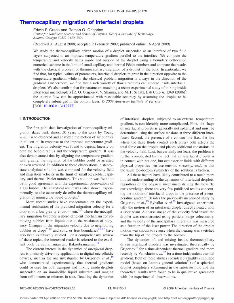
As Fig. 4�b� illustrates, the condition number becomesvery large for slender droplets, like that shown in Fig. 2�b�.As a result, the boundary collocation scheme fails to producean accurate solution at high truncation orders for slenderdroplets, as Figs. 4�a� and 5�a� show. Furthermore, Fig. 5�a�shows that our boundary collocation scheme also has diffi-culties at higher truncation orders for highly asymmetric

FIG. 4. The dependence of the residual ET �a� and condition number �b� onthe droplet aspect ratio ��12=0 corresponds to spherical droplet and �12=2to a slender film�.



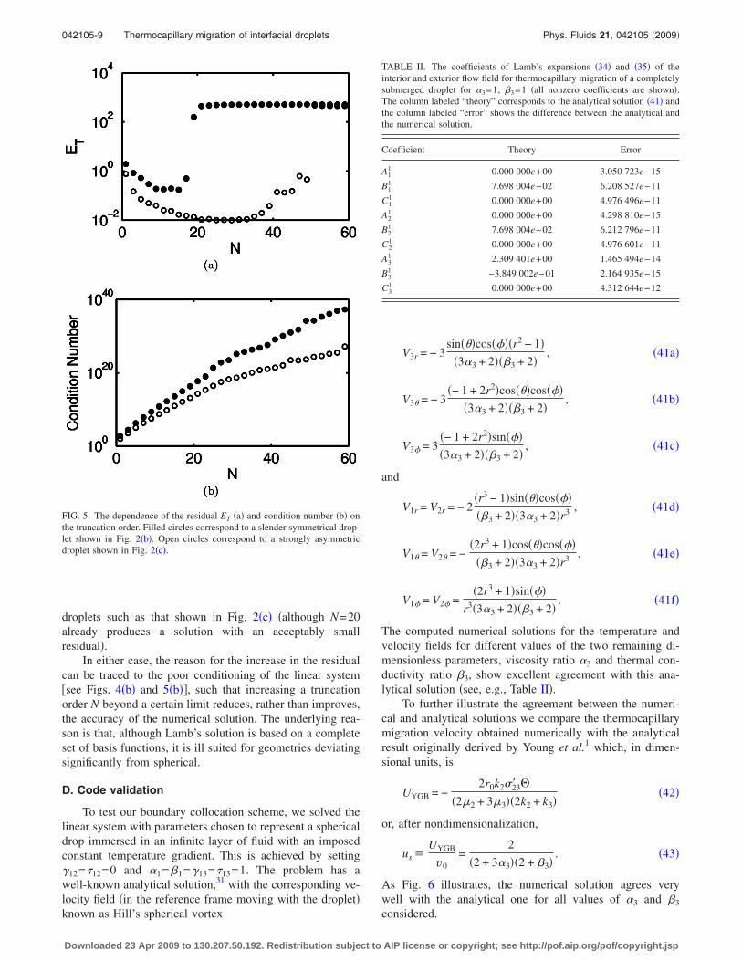
droplets such as that shown in Fig. 2�c� �although N=20already produces a solution with an acceptably smallresidual�.

In either case, the reason for the increase in the residualcan be traced to the poor conditioning of the linear system�see Figs. 4�b� and 5�b��, such that increasing a truncationorder N beyond a certain limit reduces, rather than improves,the accuracy of the numerical solution. The underlying rea-son is that, although Lamb’s solution is based on a completeset of basis functions, it is ill suited for geometries deviatingsignificantly from spherical.

D. Code validation

To test our boundary collocation scheme, we solved thelinear system with parameters chosen to represent a sphericaldrop immersed in an infinite layer of fluid with an imposedconstant temperature gradient. This is achieved by setting�12=�12=0 and �1=�1=�13=�13=1. The problem has awell-known analytical solution,31 with the corresponding ve-locity field �in the reference frame moving with the droplet�known as Hill’s spherical vortex

V3r = − 3sin��cos��r2 − 1�

�3�3 + 2��3 + 2�, �41a�

V3� = − 3�− 1 + 2r2�cos��cos��

�3�3 + 2��3 + 2�, �41b�

V3� = 3�− 1 + 2r2�sin��3�3 + 2��3 + 2�

, �41c�

and

V1r = V2r = − 2�r3 − 1�sin��cos��3 + 2��3�3 + 2�r3 , �41d�

V1� = V2� = −�2r3 + 1�cos��cos��

��3 + 2��3�3 + 2�r3 , �41e�

V1� = V2� =�2r3 + 1�sin��

r3�3�3 + 2��3 + 2�. �41f�

The computed numerical solutions for the temperature andvelocity fields for different values of the two remaining di-mensionless parameters, viscosity ratio �3 and thermal con-ductivity ratio �3, show excellent agreement with this ana-lytical solution �see, e.g., Table II�.

To further illustrate the agreement between the numeri-cal and analytical solutions we compare the thermocapillarymigration velocity obtained numerically with the analyticalresult originally derived by Young et al.1 which, in dimen-sional units, is

UYGB = −2r0k2�23� �

�2�2 + 3�3��2k2 + k3��42�

or, after nondimensionalization,

us �UYGB

v0=

2

�2 + 3�3��2 + �3�. �43�

As Fig. 6 illustrates, the numerical solution agrees verywell with the analytical one for all values of �3 and �3

considered.

FIG. 5. The dependence of the residual ET �a� and condition number �b� onthe truncation order. Filled circles correspond to a slender symmetrical drop-let shown in Fig. 2�b�. Open circles correspond to a strongly asymmetricdroplet shown in Fig. 2�c�.

TABLE II. The coefficients of Lamb’s expansions �34� and �35� of theinterior and exterior flow field for thermocapillary migration of a completelysubmerged droplet for �3=1, �3=1 �all nonzero coefficients are shown�.The column labeled “theory” corresponds to the analytical solution �41� andthe column labeled “error” shows the difference between the analytical andthe numerical solution.

Coefficient Theory Error

A11 0.000 000e+00 3.050 723e−15

B11 7.698 004e−02 6.208 527e−11

C11 0.000 000e+00 4.976 496e−11

A21 0.000 000e+00 4.298 810e−15

B21 7.698 004e−02 6.212 796e−11

C21 0.000 000e+00 4.976 601e−11

A31 2.309 401e+00 1.465 494e−14

B31 −3.849 002e−01 2.164 935e−15

C31 0.000 000e+00 4.312 644e−12



IV. RESULTS AND DISCUSSION

Next we use the boundary collocation method describedpreviously to determine the velocity of thermocapillary mi-gration for interfacial droplets and the flow fields, inside andoutside the droplet, arising in response to the applied tem-perature gradient.

A. Temperature field

Although the temperature field is not of direct interesthere, it is important for describing the relative magnitudes ofthermocapillary stresses at the surfaces of the droplet and thesubstrate. Qualitatively, the structure of the temperature fieldis controlled by the thermal conductivity ratios �1 and �3.

In particular, �1=k1 /k2 controls the relative magnitude�and uniformity� of the thermocapillary stresses at the drop-let’s top and bottom surface. As Figs. 7�a� and 7�b� illustrate,for �1�1 the temperature gradient at the top of the droplet issmaller, while for �1�1 it is larger, than at the bottom. Cor-respondingly, the thermocapillary stresses at the top domi-nate for �1�1 and those at the bottom dominate for �1�1.It should be mentioned that, although the overall temperaturedrop across the top and the bottom cap is exactly the sameregardless of �1 �T1=T2=T3 everywhere on the contact line�,it is the regions near the top and the bottom of the dropletthat have the largest contribution to the surface force �30�.

The second ratio �3=k3 /k2 controls the importance ofthermocapillary stresses at the droplet surface relative tothose at the substrate surface. Figures 7�c� and 7�d� show thatfor �3�1 the thermal gradient at the droplet surface in-creases above its value at the substrate surface away from thedroplet, while for �3�1 the thermal gradient on the dropletsurface decreases below that value. In particular, for�3→� the temperature becomes constant throughout thedroplet and the thermocapillary stress on the droplet surfacevanishes.

The remaining parameters that affect the temperaturefield are those that define the droplet shape. We found thatvarying these parameters always resulted in a temperaturefield that resembled one of the four types shown in Fig. 7.

B. Thermocapillary migration velocity

In the classical problem of thermocapillary migration,the droplet velocity �42� is essentially determined by thethermocapillary effect at the droplet surface, with the sub-strate fluid being essentially at rest far from the droplet. Forsubstrates with a free surface, the substrate itself comes inmotion due to the thermocapillary effect at its free surface.The characteristic velocity due to the thermocapillary effectat the substrate surface is V1

��v0 �in the −x direction�,while that due to the thermocapillary effect at droplet surfaceis v0 �in the +x direction�, smaller by a factor of �=H /r0.Since for interfacial droplets the ratio � is typically quitelarge, the dominant contribution to the thermocapillary mi-gration speed U0 is given by the advection of the droplet bythe substrate flow �12b� rather than the thermocapillary effectat the droplet surface. Moreover, an interfacial droplet wouldmove in the direction opposite to the applied temperaturegradient, while the classical thermocapillary migration is inthe direction of the gradient.

Since the contribution of the thermocapillary effect onthe droplet surface is much smaller than that on the substratesurface, the variation in the thermocapillary migration veloc-ity with parameters is the easiest to describe in terms of themobility function

Mi �U0 − V1

�

UYGB, �44�

where V1� is the velocity of the asymptotic flow at the sub-

strate surface. The mobility function represents the magni-

FIG. 6. The migration velocity dependence on �3 with �3=1 �a� and on �3

with �3=1 �b�. The solid curves correspond to analytical solution �43� andthe symbols represent solutions found numerically.

FIG. 7. Temperature field in the y=0. The darker shading corresponding tocooler fluid with 20 isotherms evenly spaced over the range of temperature�−Tmax,Tmax�. The parameters are �12=0.5, �13=1 and �a� �1=0.09, �3=1,Tmax=1.66, �b� �1=10, �3=1, Tmax=1.78, �c� �3=0.09, �1=1, Tmax=1.84,and �d� �3=10, �1=1, Tmax=1.60.



tude of the thermocapillary migration speed of an interfacialdroplet, with the advection component subtracted off, rela-tive to the classical thermocapillary migration velocity. De-viations of Mi from unity demonstrate the effects of confine-ment at an interface, the droplet shape variation, and thediscontinuity in the physical properties of the surroundingfluid on thermocapillary migration speed in a form indepen-dent of the substrate depth H and the droplet size r0.

There are too many nondimensional parameters to ex-plore the migration velocity of an interfacial droplet compre-hensively. Therefore, we chose to restrict our focus to thedependence of the mobility function Mi on each of the eightO�1� nondimensional parameters, with the other seven heldfixed. All the fixed parameters were set to unity except �12,the nondimensional surface tension at the interface ��12. Avalue of �12=0.5 was chosen to yield an interfacial dropletwith moderate, compared to a perfect sphere, deformation�see Fig. 7�.

We start by examining the dependence on the bulk prop-erties of the fluids, the viscosity and thermal conductivityratios. As Fig. 8�a� illustrates, an increase in the viscosityratio �1=�1 /�2 results in a decrease in Mi. This trend is dueto the increased viscous drag at the top cap of the droplet forlarge �1: as �1 increases with all other parameters fixed,U0−V1

� decreases, while UYGB does not change.A more quantitative description can be obtained by rep-

resenting the migration velocity as a sum of three compo-nents

U0 = V1� + Utc + Ush, �45�

where V1� describes the advection by the asymptotic flow, Utc

is a correction due to the thermocapillary effect at the dropletsurface, and Ush is a correction due to the shear in the sub-strate fluid �which is itself a result of the thermocapillaryeffect at the substrate interface ��12�. The component Utc

can be estimated by using a modification of the classicalexpression �42�, where the material parameters describingthe fluid surrounding the droplet are replaced with the aver-ages of the corresponding parameters for fluids 1 and 2:

Utc = −r0��13� + �23� ��k1 + k2�

2��1 + �2 + 3�3��k1 + k2 + k3�. �46�

The contribution Ush can be estimated by adapting the ex-pression for the sedimentation velocity of a liquid droplet;the well-known Hadamard–Rybczyński problem32,33

Ush = − Cr0��12� ��1 + �2 + 2�3�

2�2��1 + �2 + 3�3�, �47�

where C is a geometric factor describing the degree of sub-mersion of the droplet into the substrate fluid and the valuesof material parameters for the surrounding fluid were re-placed with the averages of those for fluids 1 and 2. Substi-tuting these expressions into the definition of the mobilityfunction one obtains

Miest =

�1 + �13��2 + 3�3��1 + �1��2 + �3�4�1 + �1 + 3�3��1 + �1 + �3�

+ C�12�1 + �1 + 2�3��2 + 3�3��2 + �3�

2�1 + �1 + 3�3��1 + �1�. �48�

Comparing the numerical result with estimate �48� we findrather good agreement, except for a small decrease in Mi at�1→0, which is likely due to a subtle flow rearrangementaround the droplet. Here and below we set C=1 /3. Thisvalue of C was chosen such that, when all parameters are setto one, both terms in Eq. �48� are equal to unity. In effect,this sets the nondimensionalized versions of Eqs. �46� and�47�, the thermocapillary and shear corrections to the migra-tion velocity, equal to each other when the material param-eters of the substrate and covering fluid are equal.

The dependence of Mi on the thermal conductivity ratio�1=k1 /k2 shown in Fig. 8�b� is also in reasonable agreementwith estimate �48�. As k1 is increased �decreased�, with allother parameters fixed, the thermocapillary effect at the topof the droplet starts to dominate �lag� that at the bottom�recall the discussion in Sec. IV A�, leading to an increase�decrease� in the thermocapillary migration speed of thedroplet relative to the substrate fluid�s�. The dependence on�1 is rather weak, reflecting the weak dependence of thethermal gradients on �1 �see Fig. 7�.

The dependence of Mi on the viscosity ratio �3=�3 /�2

is shown in Fig. 8�c�. We again find reasonable agreementwith Eq. �48� for all values of �3. For small �3, Mi ap-proaches a constant. In the limit �3→� �or �3→� with allother parameters fixed� both UYGB and Utc vanish; the ther-mocapillary migration speed of the droplet relative to the

FIG. 8. The mobility function dependence on the bulk material parameters.The symbols show the numerical results for the interfacial droplet and thesolid curve estimate �48�.



substrate is dominated by the shear flow in the substrate andapproaches a constant. In this limit Eq. �48� yields Mi�3.The dependence of Mi on the thermal conductivity ratio�3=k3 /k2 �see Fig. 8�d�� can be understood using the sameargument, which predicts Mi=const for small �3 andMi�3 for large �3.

The same argument also explains the dependence of Mi

on the surface tension temperature coefficient ratio�12=�12� /�23� shown in Fig. 9�c�. Here Eq. �48� predictsMi=const for small �12 when the thermocapillary effect atthe interface ��12 is negligible. Note that the numerical com-putation yields Mi�1 for �12→0 �just as it should be for anearly spherical droplet when Utc�UYGB�Ush�. For large�12 when the thermocapillary effect at the interface ��12 isdominant, Eq. �48� yields Mi�12, in agreement with thenumerical result.

The dependence of the mobility function on the secondsurface tension temperature coefficient ratio �13=�13� /�23� isshown in Fig. 9�d�. It is also accurately described by estimate�48� for all values of �13 and can be understood using thesame arguments used previously to explain the dependenceon �1.

We conclude this section by discussing the dependenceof the mobility function on the surface tension ratios�12= �12 / �23 and �13= �13 / �23. These ratios determine thedroplet shape and position relative to the substrate surface��12 �see Sec. II D�. No simple analytical argument can beused to predict this dependence quantitatively, so one has toresort to qualitative arguments. In particular, as �12 increasesfrom zero, the droplet shape deviates progressively from a

sphere to a slender symmetric �for �13=1� liquid lens �seeFig. 10�. The resulting increase in the surface-to-volume ra-tio leads to an increase in the viscous drag and a correspond-ing decrease in the contribution of the thermocapillary effecton the droplet surface to the migration speed, leading to adecrease in Utc and hence Mi �see Fig. 9�a��.

The value of �13 controls the position of the droplet rela-tive to the substrate surface and hence the value of the geo-metrical prefactor C in Eq. �47�. For small �13 the droplet isalmost completely expelled by the substrate fluid into thecovering fluid �see Fig. 11�b��, C is small, so the shear flowin the substrate fluid has almost no contribution to the ther-mocapillary migration speed, UshUtc�UYGB. In this limitone should expect Mi�1, as the numerics confirm. As �13

increases, so does the immersion into the substrate fluid, theprefactor C, and hence Ush, explaining the trend observed inFig. 9�b�. For large �13 �see Fig. 11�a�� the droplet is almostcompletely encapsulated by the substrate, with Mi achievingnear-maximal values.

C. Interior flow field

Next we turn to the description of the flow field insideinterfacial droplets. As we mentioned previously, the topo-logical structure of this flow field is crucially important fordetermining its mixing properties. It is the easiest to charac-terize this topological structure by identifying the invariant

FIG. 9. The mobility function dependence on the interfacial material param-eters. The symbols show the numerical results for the interfacial droplet andthe solid curve estimate �48�.

FIG. 10. The droplet shape and streamlines of the flow in the y=0 plane.The value of the surface tension ratio �12=0 corresponds to a sphericaldroplet �a� and �12=1 results in a slender droplet �b�. All other parametersare fixed at unity.

FIG. 11. The droplet shape and streamlines in the y=0 plane. The droplet isalmost completely encapsulated by the substrate for �13=1.45 �a� and almostcompletely expelled for �13=0.55 �b�. In both cases �12=0.5 and all otherparameters are set to unity.



sets of the flow such as separatrix surfaces, homo- and het-eroclinic orbits, and fixed points of the flow. One question ofparticular interest is whether the deviation of the dropletshape from a sphere, and the associated discontinuity in thesurface curvature at the contact line, have a significant im-pact on the flow topology, as compared with the flow in acompletely submerged spherical droplet under similar condi-tions.

1. Comparison with the model

To gain a better understanding of the flow structure forgeneric values of parameters we will compare the numeri-cally computed solution for the interfacial droplet with theanalytical one produced by a simplified model of the flowderived in Ref. 21. In the analytical model, a spherical drop-let was assumed to be completely submerged �with its centerat a fixed distance d�r0 below the interface� in the substratefluid, hence we will refer to this system as a submergeddroplet. In the model the interior velocity was assumed to begiven by a linear superposition of the n=1 and n=2 terms inLamb’s solution �35�, the first one representing the dipolelikefield �Hill’s spherical vortex� arising due to the thermocapil-lary effect on the droplet surface and the second—a recircu-lation flow �referred to as the Taylor flow in Ref. 21� causedby the shear flow �12c� in the substrate fluid. In our notationsthe nondimensionalized interior velocity field of the sub-merged droplet is

vr = 3�1 − r2�� r cos �

2�3 + 2�12

+1

�3�3 + 2��2 + �3��sin � cos � , �49a�

v� = � r��6 − 10r2�cos2 � − 5�1 − r2� − 2�3�4�3 + 4

�12

+3�1 − 2r2�cos �

�3�3 + 2��2 + �3��cos � , �49b�

v� = − � r�1 − 5r2 − 2�3�cos �

4�3 + 4�12

+3�1 − 2r2�

�3�3 + 2��2 + �3��sin � . �49c�

The problem has the same symmetry in the presence of aconstant horizontal temperature gradient, regardless ofwhether the droplet is fully submerged or is suspended at thesurface of the substrate. The flow is mirror symmetric withrespect to the y=0 plane, which is thus both an invariantplane and a separatrix of the flow, with Vy =0 at y=0. An-other separatrix surface is the droplet surface. The flow isalso invariant with respect to reflection about the x=0 planecombined with time reversal �v→−v�, so that vy =vz=0 atx=0. Combined with the incompressibility condition �1�, thisguarantees the existence of a line of fixed points of the flow,where v=0, lying in the plane x=0. We will, therefore, con-centrate on the velocity field in the planes x=0 and y=0which contain the majority of invariant sets.

In particular, flow �49� possesses a set of �saddle� fixedpoints lying at the intersection of the y=0 plane with thedroplet surface, with the polar angle given by

�1�2 cos2 � + �3�2��3 + 1�

+3 cos �

�3�3 + 2��2 + �3�= 0. �50�

Another set of �elliptic� fixed points lies at the intersection ofthe droplet surface with the x=0 plane, with the polar anglegiven by

�1��3 + 2�cos �

2��3 + 1�+

3

�3�3 + 2��2 + �3�= 0. �51�

To calculate the locations of the fixed points for the in-terfacial drop we chose the values of relative surface tensions�12=1 and �13=1.888 for which the interfacial droplet isalmost completely submerged. �Choosing a larger value of�13 results in a solution with an unacceptably large residual.�We also set �3=1 and �1=0 to reflect the fact that in practicethe covering fluid �e.g., air or even vacuum� would typicallyhave viscosity negligible compared to that of both the dropletand the substrate. The thermal conductivity of a typical cov-ering fluid would also be small. However, we chose to set�1=�3=1 to make the temperature gradient at the dropletsurface uniform, in accordance with the assumption used inderiving the model.

The numerical results for various relative temperaturecoefficients of surface tension �12, with fixed �13=1, arefound to be in a good qualitative �and often even quantita-tive� agreement with the simple model. For instance, Figs. 12and 13 show the locations of the fixed points on the surfaceof the droplet at x=0 and y=0, respectively. For the interfa-cial drop, the fixed points are found numerically using abounded Newton’s method, while for the submerged dropletthey are obtained by solving Eq. �51�. In each case, wefind a pair of bifurcations as �12 is increased from zero.These occur at �12

ds =4 /15�0.27 and �12sn =2 /�50�0.28 in

the model of the submerged droplet and at �12ds �0.31 and

�12sn �0.41 for the interfacial drop.

For the submerged droplet we find a symmetric pair offixed points in the y=0 plane below �12

ds. A degenerate saddle-

FIG. 12. The polar angle of the fixed points on the surface of the submerged�solid line� and the interfacial drop �circles� restricted to the x=0 plane.



node bifurcation at �12ds leads to the creation of two additional

symmetric pairs of fixed points at �=� �one pair in thex=0 plane and one in the y=0 plane�. Another saddle-nodebifurcation at �12

sn corresponds to the two pairs of fixed pointsin the y=0 plane colliding and disappearing. Above thisvalue only one pair of fixed points in the x=0 plane remains,with the polar angle approaching � /2 for large �12.

For the interfacial drop we find exactly the same se-quence of bifurcations, albeit occurring at slightly differentvalues of �12. In addition, the interfacial droplet also pos-sesses a pair of fixed points at the intersection of the y=0plane with the contact line, in this case at �c�2� /9. Addi-tional fixed points might arise near the contact line as a resultof corner vortex formation at smaller values of �1+�2. Theresolution of our numerical scheme, however, does not allowus to distinguish them.

Additional evidence for the qualitative similarity of theflows is found by computing the interior streamlines in they=0 plane for the submerged and interfacial drop at differentvalues of �12. These are shown in Fig. 14. In both cases, wefind a pair of elliptic fixed points in the interior of the droplet�on the z axis� for �12��12

ds, where the flow looks topologi-cally similar to Hill’s spherical vortex. At �12

ds one of theinterior elliptic fixed points collides with the surface anddisappears. For �12��12

ds only one fixed point is found on thez axis and the flow becomes topologically similar to rigidrotation. Similarly good qualitative agreement between thefully submerged and the interfacial droplet is found in com-paring the magnitude of the velocity in the x=0 plane shownin Fig. 15 for different values of �12. In this and the followingfigures ten evenly spaced level sets of �vx� in the interval�0,Vmax� are shown, with darker shades corresponding tolarger values.

Summarizing, we find the analytical model21 based onassuming the droplet to be completely submerged in the sub-strate fluid to also provide a reasonably accurate representa-tion of the flow inside interfacial droplets almost entirelysubmerged into the substrate fluid, with only a small capexposed to an inviscid fluid �such as air� above. Conse-quently, we should expect the model to provide a reasonably

accurate description of mixing inside the interfacial dropletsas well, provided the assumptions on which it is based hold.

2. Comparison with experiment

Next we perform a more detailed analysis of the validityof our numerical model and its predictions for the values ofparameters taken from the fluid mixing experiments reportedin Ref. 19. In the microfluidic device used in that study thecovering fluid �fluid 1� was air. Fluorinert FC-70 was used asthe substrate �fluid 2� and the droplet �fluid 3� was a water/glycerin mixture. The values of most material parameterswere taken from the CRC Handbook.34 Some parameters,such as the temperature coefficients of surface tension andthe temperature gradient were estimated from indirectmeasurements. Other parameters �substrate thickness, anddroplet radius� were measured directly. A typical setup isdescribed by the following basic scales: r0=6.2�10−5 m,�=100 K /m, and v0=3.0�10−5 m /s.

FIG. 13. The polar angle of the fixed points on the surface of the submerged�solid line� and the interfacial droplet �circles� restricted to the y=0 plane.The fixed points at the contact line, �=�c, are not shown.

FIG. 14. Stream plots for a submerged ��a�, �c�, and �e�� and interfacial��b�, �d�, and �f�� drop in the y=0 plane. Panels �a� and �b� correspond to�12=0.13, �c� to �12=0.27 and �d� to �12=0.35, and �e� and �f� correspond to�12=0.50.



The values of the corresponding nondimensional param-eters are summarized in Table III. We have not quoted thevalues for Re1, Pe1, Bo1, and Ca1 for the air layer due to itssmall values of density, viscosity, and thermal conductivity.

The heat and momentum fluxes in air are too small to sig-nificantly affect the temperature and velocity fields inside thedroplet and the substrate fluid.

A quick inspection of Table III shows that most of thenondimensional parameters have the order of magnitude as-sumed in Sec. II. One notable exception is the large value ofthe Péclet number Pe2 in the substrate fluid. This means thatat large distances from the droplet heat transport isadvection—rather than diffusion—dominated and hence ourasymptotic solution �12� is inaccurate for such large tempera-ture gradients. A more accurate analysis of the asymptoticflow profile �to be presented in a subsequent publication�shows that the temperature gradient acquires a vertical com-ponent for larger values of Pe. As we discussed previously,the validity of the present numerical model can be restoredby reducing the magnitude of the temperature gradient.

In the experiment, the easiest parameter to modify was�3, the ratio of the droplet viscosity to that of the substrate.With this in mind, we have computed and compared the ve-locity field for different values of �3. For intermediate valuesof �3, the streamlines of the flow in the y=0 plane and theabsolute value of vx at x=0 are shown in Fig. 16. A quickcomparison of the numerical solution and the simplifiedmodel flow �49� shows that the two are quite similar. Inparticular, the topological structure of both flows is domi-nated by a continuous set of elliptic fixed points in the x=0plane �see Fig. 17�, anchored at the z axis near the top of thedroplet and extending all the way to the droplet surface �thebulk of the fluid circulates around the curved line represent-

FIG. 15. The absolute value of the velocity in the x=0 plane for the sub-merged droplet ��a�, �c�, and �e�� and interfacial droplet ��b�, �d�, and �f��. �a��12=0.13 and Vmax=0.30, �b� �12=0.13 and Vmax=0.29, �c� �12=0.5 andVmax=0.56, �d� �12=0.5 and Vmax=0.46, �e� �12=1 and Vmax=0.94, and �f��12=1 and Vmax=0.71.

TABLE III. Dimensionless parameters computed from Grigoriev et al.�Ref. 19�.

Viscosity �1=0.0008 �3=0.59

Thermal conductivity �1=0.036 �3=5.9

Surface tension �12=0.33 �13=1.2

Temperature coefficient �12=0.59 �13=1.2

Bond number Bo2=0.004 Bo3=0.0008

Capillary number Ca2=1�10−5 Ca3=5�10−7

Thermal Péclet number Pe2=35 Pe3=0.02

Reynolds number Re2=0.096 Re3=2�10−4

Length =4�104 �=64

FIG. 16. The interior flow field for the light glycerin/water mixture. Shownare the streamlines for the submerged �a� and interfacial �b� droplet in they=0 plane and the magnitude of vx for the submerged �c� and interfacial �d�droplet in the x=0 plane. Vmax=0.58 and 0.33 in �c� and �d�, respectively.The parameters are as in Table III.



ing this set�. One should, therefore, expect the model to pro-vide a qualitatively accurate description of the flow �andhence its mixing properties� almost everywhere inside theinterfacial droplet.

On the other hand, one finds that the simplified model,for the same values of parameters, does not capture somefiner details of the flow near the droplet surface, such as thepairs of spiral and saddle fixed points �see Fig. 18�a�� and theheteroclinic orbits connecting the spiral fixed points �seeFig. 17�. The emergence of such invariant structures can, inprinciple, radically alter the mixing properties of the flow,either enhance or impede mixing, near the surface �and pos-sibly near the y=0 plane�. In practice, however, the regionswhere the predictions of the model disagree with the numer-ics are characterized by small values of the velocity, so ineither case the flow will have poor mixing properties there.To be fair, we should also mention that, for slightly differentvalues of parameters, similar spiral flow structures arise nearthe droplet surface in the simplified model, as Fig. 18�b�illustrates.

The corresponding numerical solution for the flow out-side the droplet is shown in Fig. 19�a�. Two features of thisflow are worth pointing out. First of all, for the values ofparameters in Table III there are two stagnation points of theflow at the front of the droplet and two at the back �moretypically one finds one stagnation point at the front and one

at the back�. The top pair corresponds to the triple contactline, while the bottom pair corresponds to a saddle located inthe vicinity of the spiral fixed point shown in Fig. 18�a� andits mirror image on the other side of the droplet. Second, thedisturbance in the exterior field due to the presence of thedroplet is seen to decay very quickly with the distance to thedroplet, such that even near the droplet the outside flow isquite close to the asymptotic shear flow V�. It, therefore,should not be very surprising to find that the thermocapillarydriven flow shown in Fig. 19�a� is qualitatively similar to theflow inside and around an interfacial droplet driven by exter-nal shear �compare with Fig. 6 of Ref. 24�.

For a small value of the relative viscosity, �3=0.043,corresponding to a pure water droplet, the numerical solutionand the flow predicted by model �49� are shown in Fig. 20.Again we find reasonable qualitative agreement over most ofthe droplet interior.

For a heavy glycerine/water mixture used in Ref. 19 thedroplet is substantially more viscous than the substrate fluid,�3=4.9. The corresponding solutions are shown in Fig. 21.In this limit too, we find reasonable qualitative agreementbetween the numerical and the approximate analytical solu-tion over most of the droplet interior. However, while the

FIG. 17. Invariant sets of the flow inside �a� the interfacial droplet and �b�the fully submerged droplet. The open squares represent the set of ellipticfixed points in the x=0 plane. The solid lines are sample 3D steamlines andthe dashed line is a heteroclinic orbit connecting the stable and unstablespiral fixed points. The surface of the droplet �light gray�, the y=0 plane�dark gray�, and the contact line are also invariant sets.

FIG. 18. Streamlines of the flow in the y=0 plane. �a� The blowup of Fig.16�b� near a spiral fixed point. �b� A spiral fixed point of the flow producedby the model for �3=0.59 and �13=0.125.

FIG. 19. The exterior flow field for the interfacial droplet with the param-eters taken from Table III. Shown are 2D streamlines in the y=0 plane �a�and sample 3D streamlines near the droplet surface �b�.



model predicts the flow to be almost identical to solid rota-tion around the y axis �i.e., quasi-2D�, the boundary condi-tions at the triple contact line force the numerical solutioninside the interfacial droplet to retain a distinctly three-dimensional �3D� structure, as the level sets of vx shown inFig. 21�d� illustrate.

To conclude this section, we would like to point out thatthe parameter space of the problem is too large to fully ex-plore. However, changing even just one of the parametersrelative to the experimental values can produce interior flowswith substantially more complex structure. One such flow ispresented in Fig. 22. In contrast to the other cases consideredin this section, we now find that the flow is organized aroundtwo sets of fixed points in the x=0 plane extending from thez axis to the surface of the droplet �see Fig. 23�a��. While thebottom set is again composed of elliptic fixed points, the top

FIG. 20. The interior flow field for a pure water droplet. Shown are thestreamlines for the submerged �a� and interfacial �b� droplet in the y=0plane and the magnitude of vx for the submerged �c� and interfacial �d�droplet in the x=0 plane. Vmax=0.75 and 2.55 in �c� and �d�, respectively.The parameters are as in Table III, except for �3=0.043.

FIG. 21. The interior flow field for the heavy glycerine/water mixture.Shown are the streamlines for the submerged �a� and interfacial �b� dropletin the y=0 plane and the magnitude of vx for the submerged �c� and inter-facial �d� droplet in the x=0 plane. Vmax=0.37 and 0.15 in �c� and �d�,respectively. The parameters are as in Table III, except for �3=4.9.

FIG. 22. Interior flow with complex topology. Shown are streamlines in they=0 plane. The parameters are as in Table III, except for �13=6�10−3.

FIG. 23. Invariant structures of the flow are shown for the interfacial �a� andthe submerged droplet �b�. The open squares and crosses represent the setsof elliptic and saddle fixed points, respectively, in the x=0 plane. The solidlines are sample 3D streamlines and the dashed line is a heteroclinic orbitconnecting the stable and unstable spiral points. The invariant sets containedinside the y=0 plane are not shown. The parameters are as in Table. III,except for �13=6�10−3.



set is made up of saddles near the z axis and elliptic fixedpoints near the surface. The important new feature of theflow is that the spirals now affect the flow globally, so model�49� provides an adequate description of the flow nowhereinside the droplet.

V. CONCLUSION

To summarize, we have numerically solved the problemof thermocapillary migration of a droplet �or liquid lens�suspended at a free interface of two immiscible fluids �thesubstrate and the covering fluid� in response to an imposedweak horizontal temperature gradient. The numerical methodused a boundary collocation scheme to compute the velocityand temperature fields in the three fluids in terms of Lamb’sgeneral solution and spherical harmonic expansions, respec-tively. The method was found to produce accurate �in termsof the residual� solutions for generic choices of parameters.However, the numerical solutions were found to become in-accurate, at large values of the truncation order, when thedroplet was either �i� strongly stretched due to a large surfacetension at the substrate’s free surface or �ii� almost com-pletely expelled by, or immersed in, the substrate. This wasfound to be a result of the condition number of the system ofequations representing the boundary conditions on the collo-cation rings becoming very large, illustrating the limitationsof Lamb’s/spherical harmonic expansions in geometries de-viating strongly from spherical.

We have computed the velocity of thermocapillary mi-gration for interfacial droplets as a function of the eight non-dimensional parameters and found the results to differ dra-matically from the classical problem of thermocapillarymigration in the bulk.1 Most important, for typical values ofparameters, interfacial droplets were found to migrate in thedirection opposite to the temperature gradient, while in theclassical problem migration is always in the direction of thegradient. For interfacial droplets, the migration speed is de-termined primarily by the motion of the substrate fluidcaused by the thermocapillary effect at its free surface andhence is strongly dependent on the boundary conditions forthe substrate layer. The thermocapillary effect on the dropletsurface responsible for the motion of the droplet relative tothe substrate’s free surface �see Sec. IV B� provides only arelatively small correction.

This study was largely motivated by the problem of mix-ing inside thermocapillary driven droplets. Although qualita-tive agreement was found between the experimentalobservations19 and the predictions of a simplified analyticalmodel,21 it was unclear whether the model, which assumedthe droplet to be completely submerged and hence spherical,was sufficiently accurate. The results reported here confirmthat, for relatively small deformations of the droplet shapefrom a sphere, the analytical solution provides a qualitativelyaccurate description of the flow in most of the droplet vol-ume. For strongly deformed droplets numerical solutions,such as those presented in this paper, become necessary.

Finally, we should mention that in the limit of vanishingPéclet numbers the velocity field is symmetric with respectto the x=0 plane, so that all streamlines are closed and the

flow is integrable. Mixing via chaotic advection requires thissymmetry to be broken. In the analysis of Ref. 21, symmetrybreaking resulted from assuming the temperature gradient tobe nonuniform. In fact, for temperature boundary conditionsrelevant to experiments, no such assumption is necessary.For finite Péclet numbers the temperature gradient acquires avertical component due to the advection of heat in the sub-strate, breaking the symmetry and making the flownonintergrable,35 even in the simplified model. Incorporatingthe effect of a vertical temperature gradient into the numeri-cal model is currently underway; the results will be reportedin a subsequent publication.

ACKNOWLEDGMENTS

We would like to thank Peter Mucha for his input in theearly stages of this investigation and Michael Schatz, VivekSharma, and Daniel Borrero for sharing the experimental re-sults. This material is based upon work supported by theNational Science Foundation under Grant No. 0400370. Ac-knowledgment was also made to the donors of the AmericanChemical Society Petroleum Research Fund for partial sup-port of this research.

1N. O. Young, J. S. Goldstein, and M. J. Block, “The motion of bubbles ina vertical temperature gradient,” J. Fluid Mech. 6, 350 �1959�.

2K. D. Barton and R. S. Subramanian, “The migration of liquid drops in avertical temperature gradient,” J. Colloid Interface Sci. 133, 211 �1989�.

3H. D. Smith, D. M. Mattox, W. R. Wilcox, R. S. Subramanian, and M.Meyyappan, “Experimental observation on the thermocapillary driven mo-tion of bubbles in a molten glass under low gravity conditions,” in Mate-rials Processing in the Reduced Gravity Environment of Space, Proceed-ings of the Materials Research Society Annual Meeting, Boston, MA,November 1981, edited by G. E. Rindone �North-Holland, New York,1982�, pp. 279–288.

4R. L. Thompson, K. J. DeWitt, and T. L. Labus, “Marangoni bubble mo-tion phenomenon in zero gravity,” Chem. Eng. Commun. 5, 299 �1980�.

5D. Neuhaus, “Bubble motions induced by a temperature gradient,” Natur-wiss. 73, 348 �1986�.

6G. Wozniak, “On the thermocapillary motion of droplets under reducedgravity,” J. Colloid Interface Sci. 141, 245 �1991�.

7P. H. Hadland, R. Balasubramaniam, G. Wozniak, and R. S. Subramanian,“Thermocapillary migration of bubbles and drops at moderate to largemarangoni number and moderate Reynolds number in reduced gravity,”Exp. Fluids 26, 240 �1999�.

8X. Ma, R. Balasubramaniam, and R. S. Subramanian, “Numerical simula-tion of thermocapillary drop motion with internal circulation,” Numer.Heat Transfer, Part A 35, 291 �1999�.

9M. Meyyappan, W. R. Wilcox, and R. S. Subramanian, “The slow axisym-metric motion of two bubbles in a thermal gradient,” J. Colloid InterfaceSci. 94, 243 �1983�.

10H. Wei and R. S. Subramanian, “Thermocapillary migration of a smallchain of bubbles,” Phys. Fluids A 5, 1583 �1993�.

11Y. Wang, R. Mauri, and A. Acrivos, “Thermocapillary migration of abidisperse suspension of bubbles,” J. Fluid Mech. 261, 47 �1994�.

12S. Nas, M. Muradoglu, and G. Tryggvason, “Pattern formation of drops inthermocapillary migration,” Int. J. Heat Mass Transfer 49, 2265�2006�.

13M. Meyyappan and R. S. Subramanian, “Thermocapillary migration of agas bubble in an arbitrary direction with respect to a plane surface,” J.Colloid Interface Sci. 115, 206 �1987�.

14R. M. Merritt and R. S. Subramanian, “Migration of a gas bubble normalto a plane horizontal surface in a vertical temperature gradient,” J. ColloidInterface Sci. 131, 514 �1989�.

15K. D. Barton and R. S. Subramanian, “Thermocapillary migration of a



http://dx.doi.org/10.1017/S0022112059000684

http://dx.doi.org/10.1016/0021-9797(89)90294-4

http://dx.doi.org/10.1080/00986448008935971

http://dx.doi.org/10.1007/BF00367261

http://dx.doi.org/10.1007/BF00367261

http://dx.doi.org/10.1016/0021-9797(91)90319-4

http://dx.doi.org/10.1007/s003480050285

http://dx.doi.org/10.1080/104077899275254

http://dx.doi.org/10.1080/104077899275254

http://dx.doi.org/10.1016/0021-9797(83)90255-2

http://dx.doi.org/10.1016/0021-9797(83)90255-2

http://dx.doi.org/10.1063/1.858835

http://dx.doi.org/10.1017/S002211209400025X

http://dx.doi.org/10.1016/j.ijheatmasstransfer.2005.12.009

http://dx.doi.org/10.1016/0021-9797(87)90025-7

http://dx.doi.org/10.1016/0021-9797(87)90025-7

http://dx.doi.org/10.1016/0021-9797(89)90194-X

http://dx.doi.org/10.1016/0021-9797(89)90194-X

liquid drop normal to a plane surface,” J. Colloid Interface Sci. 137, 170�1990�.

16M. Loewenberg and R. H. Davis, “Near-contact, thermocapillary migra-tion of a nonconducting, viscous drop normal to a planar interface,” J.Colloid Interface Sci. 160, 265 �1993�.

17S. H. Chen, “Thermocapillary migration of a fluid sphere parallel to aninsulated plane,” Langmuir 15, 8618 �1999�.

18R. S. Subramanian and R. Balasubramaniam, The Motion of Bubbles andDrops in Reduced Gravity �Cambridge University Press, Cambridge, UK,2001�.

19R. O. Grigoriev, V. Sharma, and M. F. Schatz, “Optically controlled mix-ing in microdroplets,” Lab Chip 6, 1369 �2006�.

20S. Rybalko, N. Magome, and K. Yoshikawa, “Forward and backwardlaser-guided motion of an oil droplet,” Phys. Rev. E 70, 046301 �2004�.

21R. O. Grigoriev, “Chaotic mixing in thermocapilary-driven microdrop-lets,” Phys. Fluids 17, 033601 �2005�.

22D. Vainchtein, J. Widloski, and R. O. Grigoriev, “Mixing properties ofsteady flow in thermocapillary driven droplets,” Phys. Fluids 19, 067102�2007�.

23H. Brenner, “The Stokes resistance of a slightly deformed sphere,” Chem.Eng. Sci. 19, 519 �1964�.

24K. A. Smith, J. M. Ottino, and M. O. de la Cruz, “Dynamics of a drop ata fluid interface under shear,” Phys. Rev. E 69, 046302 �2004�.

25F. Greco, “Second-order theory for the deformation of a Newtonian dropin a stationary flow field,” Phys. Fluids 14, 946 �2002�.

26R. V. Craster and O. K. Matar, “On the dynamics of liquid lenses,” J.Colloid Interface Sci. 303, 503 �2006�.

27V. G. Levich, Physicochemical Hydrodynamics �Prentice-Hall, EnglewoodCliffs, NJ, 1962�.

28Q. Hassonjee, P. Ganatos, and R. Pfeffer, “A strong-interaction theory forthe motion of arbitrary three-dimensional clusters of spherical particles atlow Reynolds number,” J. Fluid Mech. 197, 1 �1988�.

29P. Ganatos, R. Pfeffer, and S. Weinbaum, “A numerical-solution techniquefor three-dimensional Stokes flows, with applications to the motion ofstrongly interacting spheres in a plane,” J. Fluid Mech. 84, 79 �1978�.

30N. Sneeuw, “Global spherical harmonic analysis by least-squares and nu-merical quadrature methods in historical perspective,” Geophys. J. Int.118, 707 �1994�.

31J. L. Anderson, “Droplet interactions in thermocapillary motion,” Int. J.Multiphase Flow 11, 813 �1985�.

32J. Hadamard, “Mouvement permanent lent d’une sphere liquide et vis-queuse dans un liquide visqueux,” Acad. Sci., Paris, C. R. 152, 1735�1911�.

33W. Rybczynski, “Translatory motion of a fluid sphere in a viscous me-dium,” Bull. Acad. Sci. Cracovie 1a, 40 �1911�.

34D. R. Lide, CRC Handbook of Chemistry and Physics, 79 ed. �CRC, BocaRaton, FL, 1998.

35M. D. Bryden and H. Brenner, “Mass-transfer enhancement via chaoticlaminar flow within a droplet,” J. Fluid Mech. 379, 319 �1999�.



http://dx.doi.org/10.1016/0021-9797(90)90054-R

http://dx.doi.org/10.1006/jcis.1993.1396

http://dx.doi.org/10.1006/jcis.1993.1396

http://dx.doi.org/10.1021/la990641b

http://dx.doi.org/10.1039/b607003e

http://dx.doi.org/10.1103/PhysRevE.70.046301

http://dx.doi.org/10.1063/1.1850374

http://dx.doi.org/10.1063/1.2738846

http://dx.doi.org/10.1016/0009-2509(64)85045-4

http://dx.doi.org/10.1016/0009-2509(64)85045-4

http://dx.doi.org/10.1103/PhysRevE.69.046302

http://dx.doi.org/10.1063/1.1445182

http://dx.doi.org/10.1016/j.jcis.2006.08.009

http://dx.doi.org/10.1016/j.jcis.2006.08.009

http://dx.doi.org/10.1017/S0022112088003155

http://dx.doi.org/10.1017/S0022112078000051

http://dx.doi.org/10.1111/j.1365-246X.1994.tb03995.x

http://dx.doi.org/10.1016/0301-9322(85)90026-6

http://dx.doi.org/10.1016/0301-9322(85)90026-6

http://dx.doi.org/10.1017/S0022112098003395

Thermocapillary migration of interfacial droplets

Documents

Transcript of Thermocapillary migration of interfacial droplets