University of Central Florida University of Central Florida

STARS STARS

Electronic Theses and Dissertations, 2004-2019

2009

Thermo-mechanical Characterization Of High-temperature Shape Thermo-mechanical Characterization Of High-temperature Shape

Memory Ni-ti-pd Wires Memory Ni-ti-pd Wires

Matthew Fox University of Central Florida

Part of the Engineering Commons

Find similar works at: https://stars.library.ucf.edu/etd

University of Central Florida Libraries http://library.ucf.edu

This Masters Thesis (Open Access) is brought to you for free and open access by STARS. It has been accepted for

inclusion in Electronic Theses and Dissertations, 2004-2019 by an authorized administrator of STARS. For more

information, please contact STARS@ucf.edu.

STARS Citation STARS Citation Fox, Matthew, "Thermo-mechanical Characterization Of High-temperature Shape Memory Ni-ti-pd Wires" (2009). Electronic Theses and Dissertations, 2004-2019. 1509. https://stars.library.ucf.edu/etd/1509

THERMO-MECHANICAL CHARACTERIZATION OF HIGH-TEMPERATURE SHAPE MEMORY Ni-Ti-Pd WIRES

by

MATTHEW D. FOX B.S. University of Central Florida, 2007

A thesis submitted in partial fulfillment of the requirements for the degree of Master of Science

in the Department of Mechanical, Materials and Aerospace Engineering in the College of Engineering and Computer Science

at the University of Central Florida Orlando, Florida

Summer Term

2009

ii

© 2009 Matthew David Fox

iii

ABSTRACT

Actuator applications of shape memory alloys have typically been limited by their phase

transformation temperatures to around 100 degrees C. However, recently with a focus on

aerospace and turbomachinery applications there have been successful efforts to increase the

phase transformation temperatures. Several of these alloy development efforts have involved

ternary and quaternary elemental additions (e.g., Pt, Pd, etc.) to binary NiTi alloys.

Experimentally assessing the effects of varying composition and thermo-mechanical processing

parameters can be cost intensive, especially when expensive, high-purity elemental additions are

involved. Thus, in order to save on development costs there is value in establishing a

methodology that facilitates the fabrication, processing and testing of smaller specimens, rather

than larger specimens from commercial billets. With the objective of establishing such a

methodology, this work compares thermo-mechanical test results from bulk dog-bone tensile

Ni29.5Ti50.5Pd20 samples (7.62 mm diameter) with that of thin wires (100 μm-150 µm diameter)

extracted from comparable, untested bulk samples by wire electrical-discharge machining

(EDM). The wires were subsequently electropolished to different cross-sections, characterized

with Scanning Electron Microscopy, Transmission Electron Microscopy and Energy Dispersive

X-Ray Spectroscopy to verify the removal of the heat affected zone following EDM and

subjected to Laser Scanning Confocal Microscopy to accurately determine their cross-sections

before thermo-mechanical testing. Stress-strain and load-bias experiments were then performed

on these wires using a dynamic mechanical analyzer and compared with results established in

iv

previous studies for comparable bulk tensile specimens. On comparing the results from a bulk

tensile sample with that of the micron-scale wires, the overall thermomechanical trends were

accurately captured by the micron-scale wires for both the constrained recovery and monotonic

tensile tests. Specifically, there was good agreement between the stress-strain response in both

the martensitic and austenitic phases, the transformation strains at lower stresses in constrained

recovery, and the transformation temperatures at higher stresses in constrained recovery. This

work thus validated that carefully prepared micron-diameter samples can be used to obtain

representative bulk thermo-mechanical properties, and is useful for fabricating and optimizing

composition and thermomechanical processing parameters in prototype button melts prior to

commercial production. This work additionally assesses potential applications of high

temperature shape memory alloy actuator seals in turbomachinery. A concept for a shape

memory alloy turbine labyrinth seal is also presented. Funding support from NASA’s

Fundamental Aeronautics Program, Supersonics Project (NNX08AB51A) and Siemens Energy is

acknowledged.

v

Dedicated to my family and friends, who have

given me unwavering support, encouragement,

and advice throughout my education.

vi

ACKNOWLEDGMENTS

I would like to express my thanks and sincere gratitude to my advisor and mentor during

my graduate research at the University of Central Florida, Dr. Raj Vaidyanathan. Without his

undying drive to make every student that he advises better than they ever knew they could be, I

would not be the person I am today.

My sincere gratitude also goes out to Dr. Kevin Coffey, Dr. C Suryanarayana and Dr. Ali

Gordon for their sound advice and guidance during my graduate studies and for serving on my

defense committee. I would also like to extend my sincere thanks to all of the students in our

group who have provided great knowledge, wisdom, and most importantly, friendship, to me

during my time here at UCF as a graduate student. I would especially like to express my

gratitude to R. Mahadevan Manjeri for his great help in assisting me in all of my SEM and TEM

investigations that I have presented in this work, and Glen Bigelow for providing the raw data

for his bulk thermo-mechanical measurements of NiTiPd which I used in this work. I would also

like to acknowledge the AMPAC administrative staff, Ms. Cynthia Harle, Ms. Karen Glidewell,

Ms. Angelina Feliciano, and Ms. Kari Stiles for all of their great work, and for assisting me

throughout my graduate studies. Without them, we would all be lost and confused.

Most importantly, I would like to express my absolute love and respect for my family and

friends who have made my life so much more enjoyable and meaningful. Without their support,

guidance and love, I would never have become the person I am today, or the person I hope to be

in the future.

vii

TABLE OF CONTENTS

LIST OF FIGURES……………………………………………..........................................…….xii

LIST OF TABLES……………………………………………….........................................…..xvii

LIST OF ACRONYMS/ABBREVIATIONS………………….......................................……..xviii

CHAPTER ONE: INTRODUCTION……………………………………......................................1

1.1 Motivation………………………………………………........................................…1

1.2 Shape Memory Alloys.................................................................................................2

1.2.1 Shape Memory Effect…………….......................................……...……….4

1.2.2 Superelasticity………………………..…….....................................………6

1.3 Applications of Shape Memory Alloys…………….......................................……….7

1.4 Electrical-Discharge Machining..................................................................................9

1.5 Electropolishing.........................................................................................................10

1.6 Dynamic Mechanical Analysis…………………....................................…………..11

CHAPTER TWO: LITERATURE REVIEW…………………...............................…………….12

2.1 Phase Transformations in NiTi Alloys…….................................................……….12

2.2 Effect of Thermo-mechanical Treatment in NiTi Alloys….............................…….13

2.3 Physical Properties of NiTi Alloys…………………………...........................…….17

2.4 Mechanical Properties of NiTi Alloys…………………….............................……..17

2.5 Fabrication Techniques for NiTi Alloys………………….............................……...18

2.6 Scaling Effects in NiTi...............................................................................................19

viii

2.7 NiTiPd Alloys…........................................................................................................20

2.8 Prospective Application of HTSMA to Turbomachinery..........................................23

CHAPTER THREE: FABRICATION OF MICRON-SCALE NiTiPd WIRES...........................32

3.1 Bulk Sample Preparation...........................................................................................32

3.2 Electrical-Discharge Machining................................................................................32

3.3 Electropolishing.........................................................................................................34

3.3.1 Preparation of Electrolyte...........................................................................34

3.3.2 Electropolisher Operation...........................................................................35

3.3.3 Electropolishing Procedure.........................................................................40

CHAPTER FOUR: CHARACTERIZATION OF NiTiPd WIRES...............................................42

4.1 Scanning Electron Microscopy..................................................................................42

4.2 Transmission Electron Microscopy...........................................................................43

4.3 Measurement of Fabricated Wire Cross-sections......................................................43

4.4 Dynamic Mechanical Analysis..................................................................................46

4.4.1. Equipment..................................................................................................47

4.4.1.1 Perkin Elmer Diamond DMA......................................................48

4.4.1.2 Computer – MUSE Software.......................................................49

4.4.1.3 Furnace Cooling Tank..................................................................49

4.4.1.4 Furnace Cooling Controller.........................................................50

4.4.1.5 DMA Cooling Cylinder...............................................................51

4.4.2 System Operation........................................................................................51

ix

4.4.2.1 Turning on the DMA...................................................................52

4.4.2.2 Replacing the Fixtures.................................................................53

4.4.2.2.1 Tension to Bending.......................................................54

4.4.2.2.2 Bending to Tension.......................................................57

4.4.2.3 Loading the Sample.....................................................................59

4.4.2.4 Running an Experiment...............................................................61

4.4.2.5 Turning off the DMA...................................................................64

4.4.3 Calibrating the DMA..................................................................................64

4.4.3.1 Temperature.................................................................................65

4.4.3.2 Compliance Correction................................................................67

4.4.3.3 Time Constant Correction............................................................69

4.4.3.4 Viscosity Correction....................................................................70

4.4.3.5 Probe Mass...................................................................................71

4.4.3.6 Elasticity Correction....................................................................72

4.4.3.7 F/L Gain.......................................................................................72

4.4.3.8 Tension Gain................................................................................74

4.4.3.9 Load Sensitivity Correction of Static Control Mode...................75

4.4.4 Thermo-mechanical Testing of NiTiPd Wires............................................77

4.4.4.1 Calibration Verification...............................................................77

4.4.4.2 Monotonic Tensile Testing..........................................................78

4.4.4.3 Constrained Recovery..................................................................79

x

CHAPTER FIVE: RESULTS AND DISCUSSION......................................................................82

5.1 Effects of Electrical-Discharge Machining................................................................83

5.2 Effects of Electropolishing........................................................................................87

5.3 Thermo-mechanical Testing......................................................................................93

5.3.1 Verification of Instrument Calibration........................................................93

5.3.2 Monotonic Tensile Testing.......................................................................100

5.3.3 Constrained Recovery...............................................................................105

5.4 Comparison of Micron-scale Wires to Bulk Tension Samples................................106

5.4.1 Monotonic Tensile Testing.......................................................................106

5.4.2 Constrained Recovery...............................................................................109

CHAPTER SIX: CONCEPT FOR A VARIABLE AREA LABYRINTH SEAL.......................119

6.1 Background..............................................................................................................119

6.1.1 Clearance Control in Turbine Compressors..............................................120

6.2 Proof-of-Concept.....................................................................................................122

6.2.1 Active vs. Passive Control........................................................................123

6.2.2 Actuation Methods....................................................................................125

6.3 Design Challenges and Issues..................................................................................126

6.3.1 Shape Setting of SMA Segments..............................................................126

6.3.2 Sealing between Segments........................................................................127

6.3.3 Temperature Limitations...........................................................................128

6.3.4 Cyclic Degradation...................................................................................128

xi

6.3.5 Heat Transfer............................................................................................129

6.3.6 Corrosion and Oxidation...........................................................................129

CHAPTER 7: CONCLUSIONS..................................................................................................131

REFERENCES............................................................................................................................136

xii

LIST OF FIGURES

Figure 1.1: Ability of NiTi to accommodate large strains by means of detwinning in martensite [Shaw and Kyriakides 1995]..........................................................................................3

Figure 1.2: Atomic arrangements in the Shape Memory Effect…………………………………..5 Figure 1.3: Transformation path for thermally induced phase transformation; where Ms is the

martensitic start temperature, Mf is the martensitic finish temperature, As is the austenitic start temperature, and Af

is the austenitic finish temperature……………..6

Figure 1.4: Superelastic response of NiTi........................................................................................7 Figure 1.5: Material removal schematic for wire-EDM [Hsieh et al. 2009]...................................9 Figure 2.1: Forward and reverse transformation of NiTi showing intermediate R-phase

[Elliott et al. 2002].......................................................................................................13 Figure 2.2: DSC curves for a Ti-50.85at%Ni as a function of annealing temperature [Huang and Liu 2001]..................................................................................................14 Figure 2.3: Effect of thermal cycling under an applied stress of 300MPa for a given NiTi alloy

that had been 20% cold-worked and annealed at 400°C for 15 min. [Miller and Lagoudas 2001].........................................................................................15 Figure 2.4: Effect of “training” on NiTi-based HTSMA samples [Bigelow 2008].......................16 Figure 2.5: Effect of ternary alloying on the transformation temperatures of NiTiX (X=Hf, Zr, Pt,

Pd, Au) [Noebe et al. 2006].........................................................................................21 Figure 2.6: Phase Transformation path for various NiTiPd compositions [Otsuka and Wayman 1998]........................................................................................22 Figure 2.7: Stress-strain response of superelastic Ti51Pd30Ni19

[Wu and Tian 2003]..................23

Figure 2.8: Schematic of jet engine and typical operating conditions [Webster 2003].................24 Figure 2.9: Potential Applications for SMA in Turbomachinery [Bigelow 2006]........................25 Figure 2.10: Power/weight ratios for common actuator systems...................................................26

xiii

Figure 2.11: Linear SMA actuator design concept [Lam et al. 2007]...........................................27 Figure 2.12: Designs proposed in patent detailing active clearance control, with suggested

modifications for incorporation of shape memory alloys shown in red [Evans 1993].............................................................................................................28 Figure 2.13: Design proposed in patent detailing active clearance control, with suggested

modifications for incorporation of shape memory alloys shown in red [Tseng and Hauser 1991]..........................................................................................29 Figure 2.14: Design proposed in patent detailing passive clearance control, with suggested

modifications for incorporation of shape memory alloys shown in red [Diakunchak 2005]....................................................................................................29 Figure 2.15: Design proposed in patent detailing variable geometry exhaust, with suggested

modifications for incorporation of shape memory alloys shown in red [James 1980].............................................................................................................30 Figure 2.16: Design proposed in patent detailing variable geometry exhaust, with suggested

modifications for incorporation of shape memory alloys shown in red [Elorriaga et al. 2000]...............................................................................................31 Figure 2.17: Design proposed in patent detailing variable geometry exhaust, with suggested

modifications for incorporation of shape memory alloys shown in red [Renggli 2007]..........................................................................................................31 Figure 3.1: Sequence for extraction of wires from bulk samples by wire-EDM...........................33 Figure 3.2: Positioning of sample holding fixture and grounding wire for electropolisher..........37 Figure 3.3: Configuration of sample holding fixture [ESMA, Inc.]..............................................37 Figure 3.4: Gauges and displays on front panel of electropolisher................................................39 Figure 3.5: Deoxidization of titanium holding clip and placement of sample back in the clip.....40 Figure 4.1: Example 3-D profile image using Laser Scanning Confocal Microscopy…………..45 Figure 4.2: Example 2-D profile of cross-section after filtering out noise....................................46 Figure 4.3: DMA Equipment.........................................................................................................47

xiv

Figure 4.4: Furnace cooling controller showing fluid level indicator lights..................................51 Figure 4.5: How to move the DMA furnace..................................................................................54 Figure 4.6: Tension fixture assembled to the DMA......................................................................56 Figure 4.7: Fully assembled bending fixture.................................................................................56 Figure 4.8: Bending fixture assembled to the DMA......................................................................57 Figure 4.9: 20 mm steel spacer for tension fixture........................................................................59 Figure 4.10: DMA experiment sequence plot viewed in MUSE software....................................64 Figure 4.11: DMS calibration tab viewed in MUSE software.......................................................69 Figure 4.12: Schematic showing data extracted from constrained recovery experiments.............81 Figure 5.1: SEM image of wire surface after EDM.......................................................................83 Figure 5.2: EDX of oxides on wire surface after EDM.................................................................84 Figure 5.3: EDX of remelt on wire surface after EDM.................................................................84 Figure 5.4: Uniformity of wire after EDM....................................................................................85 Figure 5.5: Formation of oxide particles near surface of wire after EDM....................................85 Figure 5.6: STEM image of wire cross-section after EDM and line EDX profile........................86 Figure 5.7: SEM image of wire surface after electropolishing......................................................88 Figure 5.8: Uniformity of wire after electropolishing...................................................................88 Figure 5.9: STEM images from electropolished wire....................................................................89 Figure 5.10: TEM image of 150 μm x 130 μm wire showing absence of HAZ............................90 Figure 5.11: TEM image of 110 μm x 100 μm wire showing absence of HAZ............................90

xv

Figure 5.12: 2-D cross-section profiles of the three wires with differing corner radii tested in constrained recovery, which were generated from 3-D LSCM images....................91

Figure 5.13: 3-D surface image of wire using LSCM after electropolishing................................92 Figure 5.14: Temperature calibration results for Tg

Figure 5.15: Stress-strain response of 127 μm diameter stainless steel wire in the DMA............95

of PMMA in the DMA................................94

Figure 5.16: Stress-strain response of 127 μm diameter AlMgSi wire in the DMA.....................96 Figure 5.17: Stress-strain response of 178 μm diameter superelastic NiTi wire in the DMA.......97 Figure 5.18: Comparison of constrained recovery of commercial HTSMA wire at a hold stress of

172 MPa (reference curves from manufacturer and the DMA response of the wire after electropolishing to reduce size)........................................................................99

Figure 5.19: Stress-strain response of wires at Mf-50o

C.............................................................101

Figure 5.20: Stress-strain response of wires at Af+50o

C.............................................................102

Figure 5.21: Stress-strain response of 150 μm x 130 μm wires at Af+50oC and Af+100o

C.......103

Figure 5.22: Stress-strain response of 110 μm x 100 μm wires at Af+50oC and Af+100o

C.......104

Figure 5.23: Comparison of the stress-strain response of NiTiPd wires and the bulk sample; tested at Mf-50o

C....................................................................................................107

Figure 5.24: Comparison of the stress-strain response of NiTiPd wires and the bulk sample; tested at Af+50o

C....................................................................................................108

Figure 5.25: No-load heating of wires……………….................................................................110 Figure 5.26: Comparison of constrained recovery response of wires and the bulk sample tested at

99 MPa hold stress..................................................................................................113 Figure 5.27: Comparison of constrained recovery response of wires and the bulk sample tested at

197 MPa hold stress................................................................................................114 Figure 5.28: Comparison of constrained recovery response of wires and the bulk sample tested at

295 MPa hold stress................................................................................................115

xvi

Figure 5.29: Comparison of transformation strain with holding stress for wires and the bulk sample.....................................................................................................................116

Figure 5.30: Comparison of irrecoverable strain with holding stress for wires and the bulk

sample.....................................................................................................................117 Figure 6.1: General clearances in a jet turbine during flight [Chupp et al. 2006].......................120 Figure 6.2: General design for proof-of-concept.........................................................................123 Figure 6.3: SMA phase path for both passive and active/passive control...................................125 Figure 6.4: Methods of actuation for SMA labyrinth seal...........................................................126 Figure 6.5: Method for producing desired pre-stress for SMA segments....................................127

xvii

LIST OF TABLES Table 2.1: Fatigue of NiTi [Stöckel 1992].....................................................................................16

Table 2.2: Physical Properties of NiTi [Dynalloy]........................................................................17

Table 2.3: Mechanical Properties of NiTi [Mavroidis 2002]........................................................18

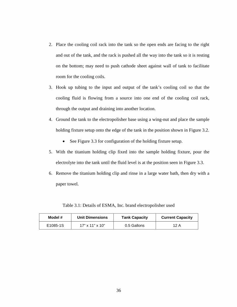
Table 3.1: Details of ESMA, Inc. brand electropolisher used.......................................................36

Table 4.1: DMA Specifications [Perkin Elmer]............................................................................48

Table 5.1: Comparison of moduli in DMA....................................................................................98

Table 5.2: Comparison of commercial HTSMA wire (reference values from manufacturer and DMA response of electropolished wire)....................................................................100

Table 5.3: Average corner radius of electropolished wires tested in constrained recovery........105

Table 5.4: Comparison of the critical stress for detwinning in martensite and the yield stress of austenite for the wire and bulk samples.....................................................................109

Table 5.5: Transformation temperatures acquired during heating...............................................110

Table 5.6: Transformation temperatures as a function of applied stress in constrained recovery for the three different micron-scale wires tested in the DMA, and the bulk sample tested on an MTS servo-hydraulic load frame...........................................................118

Table 5.7: Open-loop strain (εOL), transformation strain (εTF

), and work output as a function of applied stress in constrained recovery for the three different micron-scale wires tested in the DMA, and the bulk sample tested on an MTS servo-hydraulic load frame..........................................................................................................................118

xviii

LIST OF ACRONYMS/ABBREVIATIONS

Af

A

Austenite Finish

s

BSE Back Scattered Electron

Austenite Start

CNC Computer Numerical Controlled

DARPA Defense Advanced Research Projects Agency

DMA Dynamic Mechanical Analysis/Analyzer

DSC Differential Scanning Calorimetry

EDM Electrical-discharge Machining

EDS Energy Dispersive Spectroscopy

EDX Energy Dispersive X-ray Spectroscopy

FIB Focused Ion Beam

HAZ Heat-affected Zone

HTSMA High-temperature Shape Memory Alloy

LED Light Emitting Diode

LSCM Laser Scanning Confocal Microscopy/Microscope

Md

M

Martensite Desist

f

M

Martensite Finish

s

NASA National Aeronautics and Space Administration

Martensite Start

xix

PMMA Poly-methyl Methacrylate

RMS Root-mean Square

SE Superelasticity

SEM Scanning Electron Microscopy

SMA Shape Memory Alloy

SME Shape Memory Effect

STEM Scanning Transmission Electron Microscopy

TEM Transmission Electron Microscopy

1

CHAPTER ONE: INTRODUCTION

NiTi shape memory alloys SMA have the ability to undergo a reversible, thermoelastic

phase transformation between a low-temperature (B19’) martensite phase and a high-temperature

(B2) austenite phase. The martensite phase has a crystallographically twinned structure that can

accommodate large strains by detwinning, and when heated to the (B2) austenite structure will

return to the original macroscopic shape it had prior to deformation, even against an externally

applied stress. This ability allows NiTi to be used in actuator applications, where it can perform

work during the reverse transformation from martensite to austenite. Binary NiTi alloys are the

most commonly used shape memory alloys in commercial actuator applications, though the

transformation temperatures of binary NiTi do not exceed 120°C [Otsuka & Wayman 1998].

NiTi-based shape memory alloys have received much attention for their potential application in

the fields of aerospace and turbomachinery engineering [Rey et al. 2001, Padula et al. 2007,

Lattime & Steinetz 2002], though raising the operating temperature of these NiTi-based alloys is

needed to make them operable as actuators in the environments present in some of those

applications.

1.1 Motivation

Alloying can significantly raise the transformation temperatures of NiTi, and both

platinum and palladium have been considered some of the most promising ternary additions to

NiTi for increasing these transformation temperatures [Noebe et al. 2006]. In order to certify the

use of ternary NiTi-(Pd, Pt) alloys in actuators, they have to first be evaluated for their thermo-

2

mechanical performance [Bigelow et al. 2008], though the cost of producing large billets with

upwards of 40 at% (Pd, Pt) can prove very expensive. Establishing a methodology that

optimizes the compositional and thermo-mechanical processing parameters on small-scale button

melts (~30 g) prior to large-scale commercial production would save money on developmental

costs of novel high-temperature shape memory alloys. Such a methodology would require a

comparative study between thermo-mechanical data sets from both bulk specimens machined out

from large billets and micron-scale wires extracted from much smaller button melts, which is the

primary focus of this work. In the process of achieving the above mentioned objective, any size-

scale or geometry effects that were observed between the bulk tensile specimens and micron-

scale wires were examined. This work additionally assesses some potential areas in

turbomachinery where HTSMA actuator seals can be implemented. A concept for a shape

memory turbine labyrinth seal is also presented.

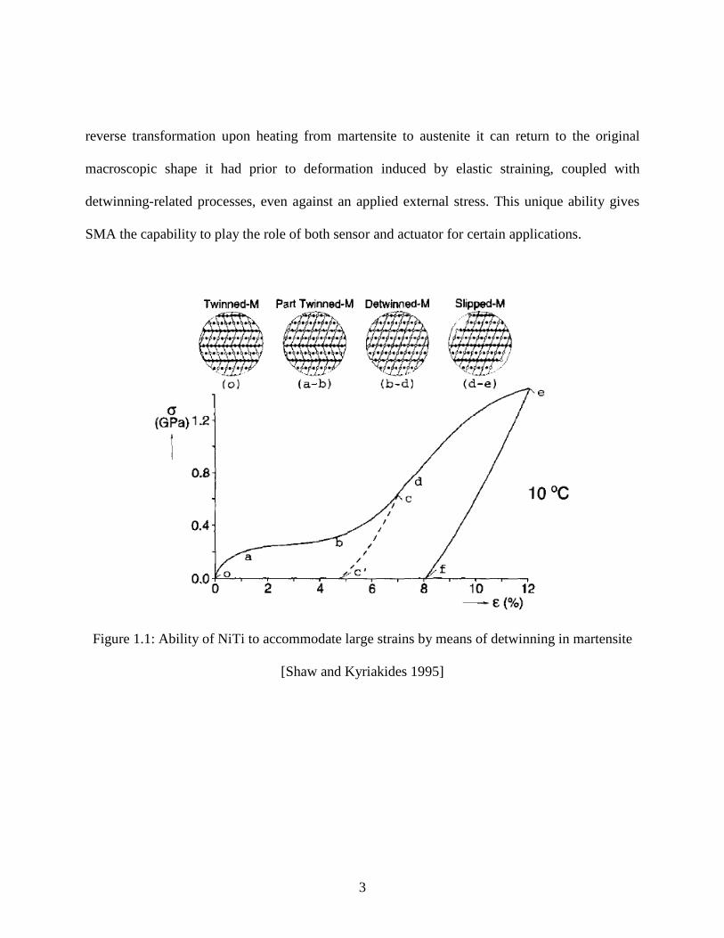
Shape memory alloys (SMAs) are a unique group of alloys that can undergo a solid-solid

phase transformation between a low-symmetry martensite phase to a high-symmetry austenite

phase [Orgéas and Favier 1998]. The crystallographically twinned martensite phase is able to

accommodate large amounts of strain by means of detwinning, which it can then recover by a

transformation to its parent phase, austenite (Fig. 1.1). This phase transformation can be

accomplished by various means; such as changing temperature, stress, or even by application of

a magnetic field for some SMAs [Otsuka & Wayman 1998]. When the SMA goes through the

1.2 Shape Memory Alloys

3

reverse transformation upon heating from martensite to austenite it can return to the original

macroscopic shape it had prior to deformation induced by elastic straining, coupled with

detwinning-related processes, even against an applied external stress. This unique ability gives

SMA the capability to play the role of both sensor and actuator for certain applications.

Figure 1.1: Ability of NiTi to accommodate large strains by means of detwinning in martensite

[Shaw and Kyriakides 1995]

4

The shape memory effect (SME) was first discovered as early as the 1930s in the Au-Cd

system, and then later discovered in the NiTi system in 1963 at the United States Naval

Ordnance Laboratories [Otsuka & Wayman 1998]. NiTi alloys are the most widely used SMAs,

as they are applied to many different fields of use; such as eyeglass frames, biomedical implants,

orthodontics, robotics, and actuators. SMAs either use the shape memory effect or

superelasticity (SE). SME can be utilized by keeping the alloy under a bias stress and cycling it

through its phase transformation temperatures to provide a designed, repeatable displacement.

SE can be utilized by stressing the alloy while it is in the austenite phase, whereby it will revert

to a stress-induced, detwinned martensite phase [Otsuka & Ren 2005]. By releasing that stress

the material will revert back to the austenite phase, and its original shape, without accumulating

any residual plasticity.

1.2.1 Shape Memory Effect

The shape memory effect arises due to a diffusion-less, solid phase transformation where

the material can be deformed in its low-temperature phase, martensite, and when heated past a

certain higher temperature will return to its original shape in the higher temperature, austenite

phase (Fig. 1.2). The “remembered” shape in the austenite phase can be chosen by the user and

trained into the material before any deformation is to take place.

5

Figure 1.2: Atomic arrangements in the shape memory effect

The transformation process is determined by the transformation temperatures of the

material. There is an austenite start temperature (As), an austenite finish temperature (Af), a

martensite start temperature (Ms), and a martensite finish temperature (Mf). This means that the

material begins transforming into one of the two phases at the start temperature, and will be

completely in that particular phase once the finish temperature is reached. If the material is

being heated to austenite it will start transforming at the As temperature and complete the

austenitic transformation at the Af temperature, and if being cooled from austenite will start

transforming into martensite at the Ms temperature and complete the martensitic transformation

at the Mf temperature (Fig. 1.3). The gap between transformation paths between the two phases

for the material is called the hysteresis. For actuator applications it is usually beneficial to have

the hysteresis be as small as possible, since quick actuation is usually desired at a given

temperature.

Austenite

Heating Cooling

Detwinned Martensite Twinned Martensite

Loading

6

Figure 1.3: Transformation path for thermally induced phase transformation; where Ms is the martensitic start temperature, Mf is the martensitic finish temperature, As is the austenitic start

temperature, and Af

is the austenitic finish temperature

Some shape memory alloys can even obtain a two-way shape memory effect, where the

alloy remembers not only its high-temperature austenite shape, but its low-temperature

martensite shape as well. This can be accomplished by many different experimental paths,

though each one links back to the creation of internal stress fields in the austenitic phase which

controls both the austenitic and martensitic phase transformations [Funakubo 1987].

1.2.2 Superelasticity

Certain shape memory alloys have the ability to behave “pseudo-elastically”, when the

alloy is at a temperature slightly above the Af. These shape memory alloys have a martensite

desist (Md) temperature that is higher than the Af temperature. This means it can accommodate

7

large strains under an applied stress by undergoing an isothermal phase transformation from the

austenite phase to a detwinned martensite structure, without the accumulation of plasticity

[Miura et al. 1986]. When the stress is released it reverts back to the austenitic phase and returns

to its original shape due to the stress-induced martensite phase no longer being energetically

stable at that temperature under no load (Fig. 1.4).

Figure 1.4: Superelastic response of NiTi

1.3 Applications of Shape Memory Alloys

The shape memory and superelastic effects are both used in various applications of

SMAs. The shape memory effect requires biasing stress and thermal fluctuations to be viable

actuators, and the superelastic effect requires the material to be in a certain temperature range to

utilize its unique properties.

8

One of the first prominent applications of SMAs using the shape memory effect was in

1971, when a low-temperature NiTiFe Cryofit coupling was applied to connect titanium piping in

a high-pressure hydraulic system on an F-14 fighter jet [Humbeeck 1999]. This successful

demonstration in 1970 can be seen as the catalyst for engineering interest in SMAs, as a

multitude of patents have since been filed that involve the use of SMAs [Wu et al. 2000].

The superelastic effect in NiTi was proposed as a viable dental arch wire material in 1986

[Miura et al. 1986]. Dental arch wires used in braces and other dental devices use NiTi-based

alloys to provide the same effect steel wires do, with less fatigue and higher reliability. Miura et

al suggested that superelastic NiTi could provide a wide range of stresses needed for these arch

wires depending on the heat treatment used for shape-setting, and was least likely to undergo

permanent deformation over time as compared to other alloys being used as dental arch wires.

Intravascular NiTi stents were first conceived of in 1983, and were tested for years on

several different species of animals for their resistance to corrosion [Ryhanen 1999]. Stents are

comprised of a wire mesh in the shape of a tube that is inserted into a clogged artery to keep the

blood flowing through what used to be a blocked, or partially blocked, area. Stents utilize the

superelastic effect by being deformed into a catheter and when it is released into an artery will

expand and push on the blockage to expand the walls of the artery to open it. Since the mid-90s

stents have been used extensively in humans, and have been scientifically proven to provide

adequate function and excellent fatigue resistance, without invasive surgery [Berg 2008].

9

1.4 Electrical-Discharge Machining

Electrical-discharge machining (EDM) is a method used to cut hard materials that would

otherwise require careful machining techniques. EDM requires the material being cut to be

electrically conductive because EDM does not machine by conventional means, but locally melts

small craters in succession using high-frequency electrical pulses between the electrode and the

material. Wire-EDM uses the same principle, except the electrode used is a wire, and can locally

melt along a line instead of a point or area (Fig. 1.5).

Figure 1.5: Material removal schematic for wire-EDM [Hsieh et al. 2009]

10

EDM produces a heat-affected zone (HAZ) on the surface of the material due to the rapid

melting and solidification of the material. The thickness and composition of this zone for NiTi-

based alloys has been shown to vary depending on the process parameters, and the surface

roughness of the samples were also shown to vary depending on these parameters [Lin et al.

2001, Theisen et al. 2004, Hsieh et al. 2009].

1.5 Electropolishing

Electropolishing is an electrochemical etching process that smoothes the surfaces of

metal parts. The part is submerged in an electrolytic bath, and serves as the anode when a direct

current is applied to the part. The tank also contains cathodes to complete the circuit. When the

current is applied, an anodic film will form on the surface of the part, with it being thicker at the

surface, and thinner on the protrusions from the surface. This means that a higher current density

will be present on the peaks and will be etched away faster than the surface, hence, smoothing

the part. Electropolishing is used on NiTi parts to debur, decrease surface roughness, provide a

shiny surface, to passivate the part, or a combination of the aforementioned. Electropolishing

medical instruments and implants are especially important. Not only does the surface need to be

completely deburred if it is going to be put into the human body, but a thin titanium dioxide film

is formed on the surface during electropolishing that acts to prevent oxidation and corrosion, and

to prevent toxic nickel from diffusing into the body. As previously mentioned in Section 1.4, the

surface roughness of a part after EDM is dependant on the process parameters. Electropolishing

11

can lower the surface roughness of a part, but the time required to achieve the desired surface

roughness is dependant on the starting roughness [Pohl et al. 2004, Theisen et al. 2004].

Electrolyte temperature can also play an important role in the material removal rate of the parts

surface [Fushimi et al. 2006, Miao et al. 2006]. Depending on the material being electropolished

different electrolyte compositions are necessary to achieve the best results. For NiTi, it has been

shown that methanolic sulfuric acid shows some of the best results [Fushimi et al. 2006, Nishiura

et al. 2007].

1.6 Dynamic Mechanical Analysis

Dynamic mechanical analysis/analyzer (DMA) can measure rheological conditions under

both dynamic and static conditions. DMA can measure the modulus, compliance and damping,

as a function of temperature, time, frequency, stress, atmosphere, or a combination of these

parameters [Perkin Elmer]. Shape memory alloys have been tested in a DMA to determine

transformation regions and damping capacity, but a DMA is not commonly utilized to

characterize the actuator-type properties of the alloy; quasi-static stress strain or constrained

recovery. Roy et al. showed that DMA is also a viable tool for assessing such properties by

testing commercially available, trained NiTi wires of diameter 0.38 mm [Roy et al. 2008]. This

work will further this development by testing novel HTSMA wires with diameters ranging from

0.10 mm – 0.15mm for their actuator-type, thermo-mechanical properties.

12

CHAPTER TWO: LITERATURE REVIEW

Nickel-titanium alloys are the most common shape memory alloys on the market. They

are used in a wide variety of applications due to both their shape memory and superelastic

properties. The operational temperature limit for these alloys cannot exceed 100°C in most

circumstances; therefore, ternary elemental additions have been experimented with to increase

these operational temperature limits. The effects of palladium and platinum addition to NiTi will

be presented further in this chapter, along with potential applications of these alloys to

turbomachinery.

2.1 Phase Transformations in NiTi Alloys

NiTi exhibits a phase transition between its high-temperature phase, (B2) austenite, to its

low-temperature phase, (B19’) martensite, and back again. The B2 lattice is of BCC structure

and the B19’ lattice is of monoclinic structure. There is also the possibility of an R-phase

forming during the forward transformation when cooling from B2 B19’ (Fig. 2.1). The R-

phase has a trigonal structure which causes little lattice distortion when formed from the B2

phase (B2 R); otherwise, larger lattice distortions are noticed when going directly from B2

B19’ or R B19’ [Kim et al. 2004].

13

Figure 2.1: Forward and reverse transformation of NiTi showing intermediate R-phase [Elliott et al. 2002]

2.2 Effect of Thermo-mechanical Treatment in NiTi Alloys

There are many ways to control the hysteresis, transformation temperatures and yield

strength of NiTi alloys. Cold-working NiTi induces dislocations in the material, which greatly

strengthens the alloy, but these dislocations also prevent detwinning when strained in the

martensitic phase, causing slip to occur prematurely. By subsequently annealing NiTi after cold-

working the SME is reintroduced, but the yield strength decreases. Overall, the process of cold-

14

working and annealing increases the yield strength of the material from what it was before any

thermo-mechanical processing.

Annealing can affect the transformation temperatures in NiTi. Annealing at increasing

temperatures from 300°C can increase the transformation temperatures, but at a certain higher

temperature the trend can reverse (Fig. 2.2). Therefore, optimizing the annealing temperature

and time for a certain alloy can prove advantageous, and give the user more control over the

properties. By annealing at certain temperatures below the recrystallization temperature an R-

phase can be induced in the alloy.

Figure 2.2: DSC curves for a Ti-50.85 at%Ni as a function of annealing temperature [Huang and Liu 2001]

Thermal cycling an alloy can also induce a two-way effect, otherwise known as

“training,” which can thermo-mechanically stabilize the material after a certain amount of

thermal cycles under an applied stress (Fig. 2.3).

15

Figure 2.3: Effect of thermal cycling under an applied stress of 300 MPa for a given NiTi alloy that had been 20% cold-worked and annealed at 400°C for 15 min. [Miller and Lagoudas 2001]

Another similar method has been established and used for training of NiTiPd-based

HTSMA tension samples by NASA Glenn Research Center [Bigelow 2008]. The samples are

thermally cycled twice under no-load to relieve any stresses that might still be in the sample from

fabrication, and then thermally cycled twice at 172 MPa to evaluate the effect of thermal cycling

at no-load. After which, the sample was thermally cycled 10 times at 345 MPa, then cycled 10

more times back at 172 MPa to see if the high-stress cycling affected the stability of the alloy at

lower stresses. The results of which can be seen in Figure 2.4. After plastically deforming the

material at 345 MPa during thermal cycling the sample was able to undergo no further residual

plasticity when thermally cycled at 172 MPa. Although, if the alloy was overheated during

operation after training it would lose all of the training it had undergone, and go back to gaining

significant residual plasticity after cycling.

16

Figure 2.4: Effect of “training” on ternary and quaternary High-temperature NiTi-based alloys [Bigelow 2008]

The controlled stress or strain on a trained NiTi sample also significantly affects the

fatigue behavior of the alloy. By actuating at lower stresses or strains the alloy has longer cycle

life (Table 2.1).

Table 2.1: Fatigue of NiTi [Stöckel 1992]

# Cycles Max. Strain Max. Stress

1 8% 500 MPa

100 4% 275 MPa

10000 2% 140 MPa

100000+ 1% 70 MPa

17

2.3 Physical Properties of NiTi Alloys

NiTi shows similar physical properties to that of nickel, one of its base elements, but does

show differences between its two different phases; martensite and austenite. Table 2.2 shows

many of the important physical properties of NiTi that are of value when designing a NiTi-based

actuator.

Table 2.2: Physical Properties of NiTi [Dynalloy]

Density 6.45 g/cc

Specific Heat 837 J/(kg·K)

Melting Point 1250°C

Thermal Conductivity 0.21 W/(cm·°C)

Martensite 6.6x10-6/°C

Austenite 11x10-6/°C

Martensite 7.0x10-7 Ω·m

Austenite 8.5x10-7 Ω·m

Thermal Expansion Coefficient

Electrical Resistivity

2.4 Mechanical Properties of NiTi Alloys

Thermo-mechanical processing of NiTi can change some of the mechanical properties;

i.e., yield strength and elongation at break. Repeatability of processing is also a factor in the

mechanical properties, as all manufacturers of NiTi publish ranges of certain properties on their

18

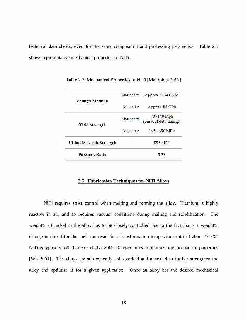
technical data sheets, even for the same composition and processing parameters. Table 2.3

shows representative mechanical properties of NiTi.

Table 2.3: Mechanical Properties of NiTi [Mavroidis 2002]

2.5 Fabrication Techniques for NiTi Alloys

NiTi requires strict control when melting and forming the alloy. Titanium is highly

reactive in air, and so requires vacuum conditions during melting and solidification. The

weight% of nickel in the alloy has to be closely controlled due to the fact that a 1 weight%

change in nickel for the melt can result in a transformation temperature shift of about 100°C.

NiTi is typically rolled or extruded at 800°C temperatures to optimize the mechanical properties

[Wu 2001]. The alloys are subsequently cold-worked and annealed to further strengthen the

alloy and optimize it for a given application. Once an alloy has the desired mechanical

19

properties it can be formed to many different shapes. In order to have a prescribed austenite

phase shape, the part can be mechanically deformed into a holding fixture and shape-set.

Typically, shape-setting is done for NiTi between 350-550°C for 5-60 min., depending on the

composition and size of the part.

Cold-drawing NiTi is a common practice in industry, but requires delicate procedures.

By passing the material through several dies to achieve the desired final dimensions, frequent

inter-pass annealing steps are performed. Inter-pass annealing refers to multiple anneals of the

wire between 600-800°C after every few reduction steps, due to the rapid work-hardening of the

NiTi wire [Wu 2001].

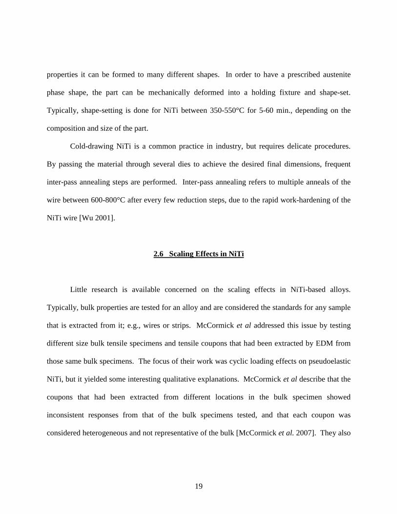
2.6 Scaling Effects in NiTi

Little research is available concerned on the scaling effects in NiTi-based alloys.

Typically, bulk properties are tested for an alloy and are considered the standards for any sample

that is extracted from it; e.g., wires or strips. McCormick et al addressed this issue by testing

different size bulk tensile specimens and tensile coupons that had been extracted by EDM from

those same bulk specimens. The focus of their work was cyclic loading effects on pseudoelastic

NiTi, but it yielded some interesting qualitative explanations. McCormick et al describe that the

coupons that had been extracted from different locations in the bulk specimen showed

inconsistent responses from that of the bulk specimens tested, and that each coupon was

considered heterogeneous and not representative of the bulk [McCormick et al. 2007]. They also

20

deduced that precipitates have a larger influence on the strength of hot-rolled NiTi than grain

size, and that Lüders-like behavior is prevalent in all the coupons, but not the full-scale tensile

specimens [McCormick et al. 2007].

2.7 NiTiPd Alloys

There are several ternary elemental additions that have been added to NiTi to increase the

transformation temperatures; such as hafnium, zirconium, platinum, palladium and gold (Fig.

2.5). These alloys typically have lower transformation temperatures than binary NiTi for the first

10% ternary addition, but then increase linearly to exceed binary NiTi [Lindquist 1988, Noebe et

al. 2006]. Though the transformation temperatures have been raised using ternary alloying, not

much thermo-mechanical testing has been done to evaluate the prospect of using the SME of

these alloys in an actuator application. Most of the ongoing research being done to assess the

actuator-type performance of HTSMA is in the NiTiPd and NiTiPt systems [Lin et al. 2008,

Bigelow 2008].

21

Figure 2.5: Effect of ternary alloying on the transformation temperatures of NiTiX (X=Hf, Zr, Pt, Pd, Au) [Noebe et al. 2006]

High-temperature NiTiPd does not have the same martensitic phase structure as binary

NiTi. For compositions of NiTiPd with <10 at% Pd the structure is monoclinic B19’ like NiTi,

but at over 10 at% Pd the martensite structure becomes orthorhombic B19 [Lindquist 1988,

Otsuka and Wayman 1998] (Fig. 2.6).

22

Figure 2.6: Phase Transformation path for various NiTiPd compositions [Otsuka and Wayman 1998]

NiTiPd also exhibits superelasticity in certain temperature ranges, but does not follow the

same stress-strain trend as NiTi (Fig. 2.7). The stress-induced B2 B19 transformation (II)

occurs very suddenly due to the reduced number of martensite variants for its orthorhombic

martensitic structure, as compared to B19’, and reorients quickly to begin elastic deformation of

the detwinned orthorhombic structure (III) [Wu and Tian 2003].

23

Figure 2.7: Stress-strain response of superelastic Ti51Pd30Ni19

[Wu and Tian 2003]

Shimizu et al. have established ageing parameters to raise the critical stress for slip,

thereby strengthening the alloy for actuator-type applications [Shimizu et al. 1998]. Tian et al.

have also been able to improve the oxidation resistance of NiTiPd by doping it with 1 wt%

Cerium, which impedes the outward diffusion of Ti to the surface [Tian et al. 2003].

2.8 Prospective Application of SMAs to Turbomachinery

Shape memory alloys have been used for many aerospace and aeronautical applications,

but not in any roles requiring high transformation temperatures (>100°C). They have been used

to extend solar panels on satellites [Carpenter et al. 1995], change the exhaust geometry on jet

24

engines [Calkins et al. 2006], and used to morph wing geometry [Lizotte and Allen 2005], but

have not been used to control flow within a turbine. Both ground-based turbines and jet engines

have internal temperatures during operation that far exceed the operational limit of any

commercially available shape memory alloy. There are many other factors besides high

temperatures that can influence the operation of an SMA material inside a turbine; i.e. high

pressures, vibrations, and creep effects from rotating components (Fig. 2.8).

Figure 2.8: Schematic of jet engine and typical operating conditions [Webster 2003]

There are many potential applications for SMAs in turbines, but the development of

viable high-temperature SMAs has not yet been established to survive in these environments (Fig.

2.9). Though an SMA-controlled jet engine inlet has been tested by DARPA, and Boeing has

developed a variable area fan nozzle prototype and a flight-tested variable geometry chevron

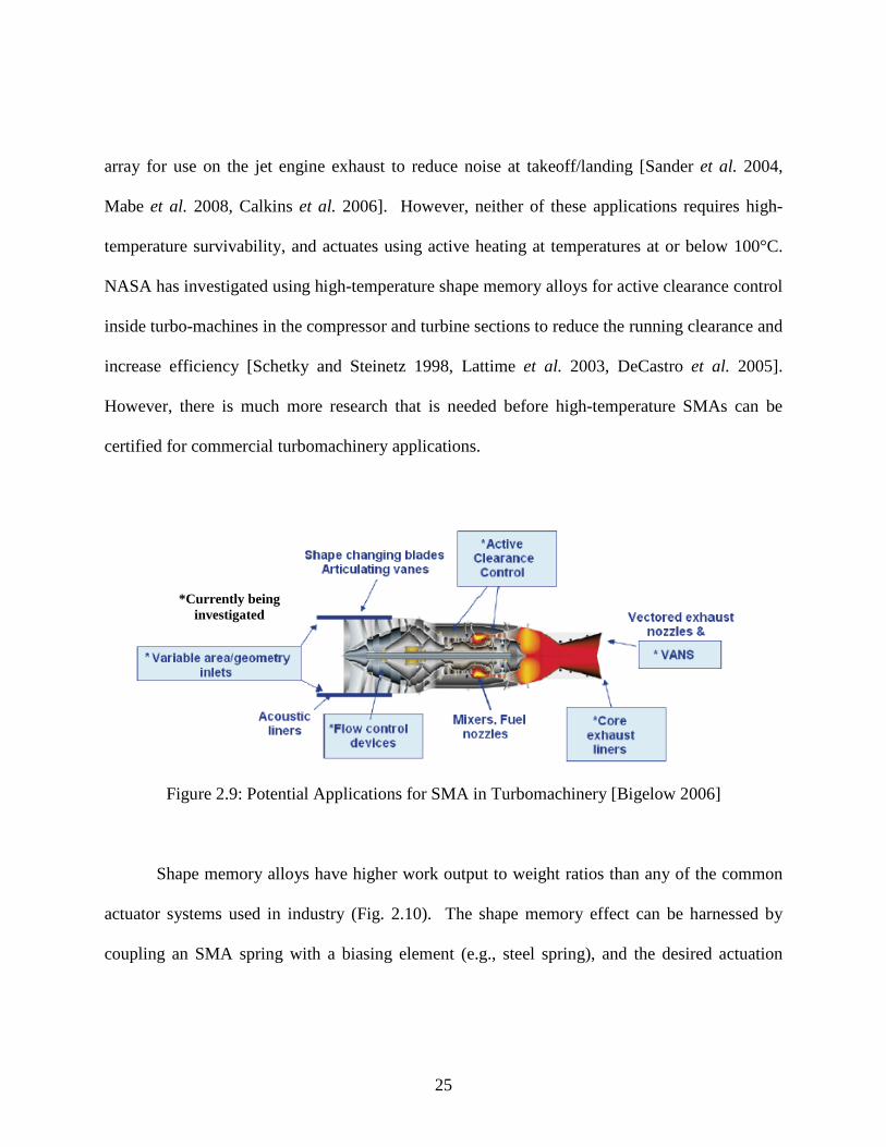
25

array for use on the jet engine exhaust to reduce noise at takeoff/landing [Sander et al. 2004,

Mabe et al. 2008, Calkins et al. 2006]. However, neither of these applications requires high-

temperature survivability, and actuates using active heating at temperatures at or below 100°C.

NASA has investigated using high-temperature shape memory alloys for active clearance control

inside turbo-machines in the compressor and turbine sections to reduce the running clearance and

increase efficiency [Schetky and Steinetz 1998, Lattime et al. 2003, DeCastro et al. 2005].

However, there is much more research that is needed before high-temperature SMAs can be

certified for commercial turbomachinery applications.

Figure 2.9: Potential Applications for SMA in Turbomachinery [Bigelow 2006]

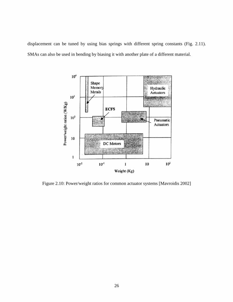
Shape memory alloys have higher work output to weight ratios than any of the common

actuator systems used in industry (Fig. 2.10). The shape memory effect can be harnessed by

coupling an SMA spring with a biasing element (e.g., steel spring), and the desired actuation

*Currently being investigated

26

displacement can be tuned by using bias springs with different spring constants (Fig. 2.11).

SMAs can also be used in bending by biasing it with another plate of a different material.

Figure 2.10: Power/weight ratios for common actuator systems [Mavroidis 2002]

27

Figure 2.11: Linear SMA actuator design concept [Lam et al. 2007]

There are many patent filings that detail the use of actuators in turbines for the purposes

of either active/passive clearance control, or variable geometry exhaust systems. None of these

have come to fruition by the use of shape memory alloys as the main component for the actuators

described.

For active clearance control, D. H. Evans has proposed using a feedback control system,

coupled with a fluid reservoir, to control the position of a shroud segment over rotating turbine

blades [Evans 1993]. By replacing the feedback control system with a shape memory alloy,

coupled with a bias spring, the same function can be achieved using less weight and simpler

28

operation (Fig. 2.12). Similarly, a unison ring can be positioned circumferentially around the

turbine blade shroud, and can rotate by active mechanical means using an external actuation

system to radially position the shroud segments towards and away from the blade tips [Tseng and

Hauser 1991]. The same function can be accomplished by using an active/passive shape

memory alloy circumferential actuator system (Fig. 2.13). A passive system proposed by I. S.

Diakunchak suggests using a bi-metal approach for clearance control [Diakunchak 2005]. This

means forming a layered structure with two opposing materials, where each one has its own

coefficient of thermal expansion that can passively alter position of the structure tips to come

closer or further from the turbine blades during heating and cooling. By using the same

approach, a shape memory alloy and a biasing material (e.g., Inconel 718) can be sandwiched

together into a composite to form a bi-metal actuator (Fig. 2.14).

Figure 2.12: Designs proposed in patent detailing active clearance control, with suggested modifications for incorporation of shape memory alloys shown in red [Evans 1993]

29

Figure 2.13: Design proposed in patent detailing active clearance control, with suggested modifications for incorporation of shape memory alloys shown in red [Tseng and Hauser 1991]

Figure 2.14: Design proposed in patent detailing passive clearance control, with suggested modifications for incorporation of shape memory alloys shown in red [Diakunchak 2005]

30

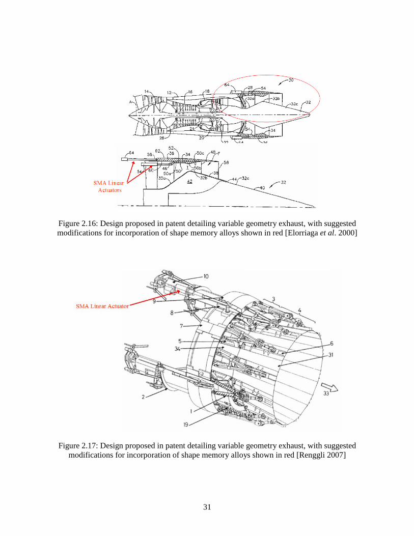
For variable geometry exhaust systems, V. L. James has proposed a mechanism which

controls the expansion ratio of a turbine exhaust by using circumferentially positioned linear

actuators to change the area of the throat [James 1980]; these linear actuators can be replaced

with an SMA linear actuator, like the one seen in Figure 2.11 (Fig. 2.15). Also, two overlapping

circumferential sleeves can be free to move backwards and forwards about the radial axis to alter

the expansion ratio by repositioning the exhaust throat along the diffuser cone by using linear

actuators [Renggli 2007]. These linear actuators can also be replaced with an SMA linear

actuator (Fig. 2.16). A similar concept has circumferentially positioned linear actuators which

control a mechanism to expand the exhaust area, while keeping the throat area and position

constant [Elorriaga et al. 2000]; these linear actuators can also be SMA-based (Fig. 2.17).

Figure 2.15: Design proposed in patent detailing variable geometry exhaust, with suggested modifications for incorporation of shape memory alloys shown in red [James 1980]

31

Figure 2.16: Design proposed in patent detailing variable geometry exhaust, with suggested modifications for incorporation of shape memory alloys shown in red [Elorriaga et al. 2000]

Figure 2.17: Design proposed in patent detailing variable geometry exhaust, with suggested modifications for incorporation of shape memory alloys shown in red [Renggli 2007]

32

CHAPTER THREE: FABRICATION OF MICRON-SCALE NiTiPd WIRES

The NiTiPd wires tested in this work were obtained by using a combination of wire

electrical-discharge machining (EDM) and electropolishing. Rectangular cross-section wires

with dimensions of 60 mm long and 0.2 mm sides were extracted from Ni29.5Ti50.5Pd20

bulk

tension specimens using wire-EDM. The cross-section dimensions were further reduced by

electropolishing to uniformly remove material from the surface, as well as remove the heat-

affected zone (HAZ) caused by EDM.

3.1 Bulk Sample Preparation

The as-received Ni29.5Ti50.5Pd20

bulk tension sample used for extracting the wires by

wire-EDM for this work was prepared using the procedure previously outlined [Bigelow 2006].

3.2 Electrical-Discharge Machining

To relieve any possible residual stresses from the machining operation of the bulk

specimens, all of the samples were wrapped in titanium foil and annealed at 400°C for one hour

and furnace cooled [Bigelow 2006]. Rectangular cross-section wire samples with cross-section

dimensions of 210 ±7 μm x 200 ±7 μm and length 60 mm were obtained from one of the “virgin”

bulk specimens by wire-EDM. An Elox-Model P wire-EDM with a Fanuc-6 controller was used

33

for the process. The controller was set to an operating voltage of 50V, a working current of 2.5A

and used a 100 μm diameter brass wire as the electrode at room temperature, and deionized water

as the dielectric fluid.

Figure 3.1: Sequence for extraction of wires from bulk samples by wire-EDM

3.3 Electropolishing

Selection of the proper electrolyte and operating voltage of the equipment was essential

to providing both good material removal rates and surface finish. Two sets of wires produced by

EDM were electropolished in a 3 mol·dm-3 methanolic sulfuric acid electrolyte [Fushimi et al.

34

2006] held at 24°C in an ESMA model E1085-1S electropolisher. One set had cross-sectional

edge lengths which averaged 150 ±2 μm x 130 ±2 μm and the other set had cross-sectional edge

lengths which averaged 110 ±2 μm x 100 ±2 μm. As a beneficial consequence of varying the

electropolishing parameters to optimize the removal rate and uniformity of the wires, a pattern

was established that could also control the relative curvature of the corners of each wire cross-

section. It has been suggested that lower electrolyte temperatures provide a better surface finish

[Fushimi et al. 2006]; however, due to the slow material removal rates that accompany it

electropolishing was performed at room temperature. The 60 mm long wires that were extracted

by wire-EDM were first cut into two 30 mm pieces before electropolishing.

3.3.1 Preparation of Electrolyte

To prepare the electrolyte 96% pure sulfuric acid and 99.8% pure methanol was used. By

creating an electrolytic solution that is 16 volume percent sulfuric acid and 84 volume percent

methanol, the desired 3 mol·dm-3 methanolic sulfuric acid was formed. The methanol was first

measured out to be 84% of the volume necessary to fill the electropolisher tank to the desired

fluid level. The remaining 16% volume of sulfuric acid was then measured out and mixed very

slowly into the methanol. The reaction of sulfuric acid with methanol is a exothermic reaction

that can easily become dangerous if precaution is not met. Care was taken to add sulfuric acid to

methanol, and not the other way around. The following is the procedure to be followed to mix

the electrolyte.

35

1. Make sure the container has a large opening (about the same diameter of the

container) to allow for more gas escape.

2. Always mix under ventilation and while wearing the appropriate safety gear

prescribed in the MSDS for sulfuric acid [Sulfuric Acid MSDS].

3. Pour the sulfuric acid very slowly into the methanol.

• Stop immediately if the bubbles begin to burst outwards from the surface.

• Small additions of sulfuric acid should be done at short intervals to allow

for the reaction to settle down before proceeding.

• The exothermic reaction of methanol and sulfuric acid produces a

combination of dimethyl sulfate and water.

4. Once the final solution is prepared and mixed allow for the full reaction to

complete and for the electrolyte to cool back to room temperature, as it will get

hotter during mixing.

3.3.2 Electropolishing Procedure

An ESMA, Inc. brand electropolisher was used to polish the wires used in this work. The

details of the model used can be seen in Table 3.1. Electropolishing was done in a ventilated

area. The following procedure was used for setup and operation of the electropolisher.

1. Place tank into the recess at the top of the electropolisher so the post on the base

plate of the polisher is aligned with the cylindrical recess in the tank.

36

2. Place the cooling coil rack into the tank so the open ends are facing to the right

and out of the tank, and the rack is pushed all the way into the tank so it is resting

on the bottom; may need to push cathode sheet against wall of tank to facilitate

room for the cooling coils.

3. Hook up tubing to the input and output of the tank’s cooling coil so that the

cooling fluid is flowing from a source into one end of the cooling coil rack,

through the output and draining into another location.

4. Ground the tank to the electropolisher base using a wing-nut and place the sample

holding fixture setup onto the edge of the tank in the position shown in Figure 3.2.

• See Figure 3.3 for configuration of the holding fixture setup.

5. With the titanium holding clip fixed into the sample holding fixture, pour the

electrolyte into the tank until the fluid level is at the position seen in Figure 3.3.

6. Remove the titanium holding clip and rinse in a large water bath, then dry with a

paper towel.

Table 3.1: Details of ESMA, Inc. brand electropolisher used

Model # Unit Dimensions Tank Capacity Current Capacity

E1085-1S 17" x 11" x 10" 0.5 Gallons 12 A

37

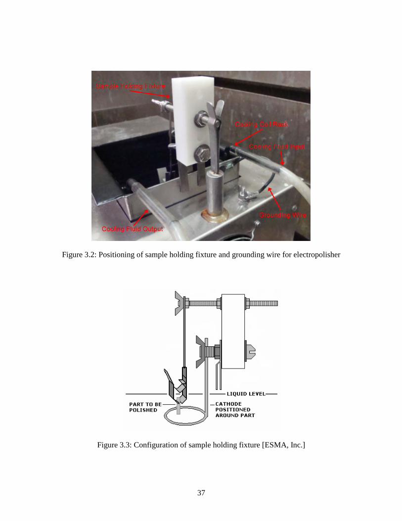
Figure 3.2: Positioning of sample holding fixture and grounding wire for electropolisher

Figure 3.3: Configuration of sample holding fixture [ESMA, Inc.]

38

7. Plug the electropolisher into a standard wall outlet, turn on the system using the

switch on the front face of the electropolisher, and set the fluid temperature using

the input panel on the face of the electropolisher (Fig. 3.4).

8. Wait for the temperature to stabilize, then fix the sample into the titanium holding

clip and fix the titanium holding clip back onto the sample holding fixture with

the sample being completely submerged in the electrolyte and centered in the

cathode ring.

9. Set the timer for the time you want to polish the sample.

10. When you are ready, hit the “Start” button, and adjust the voltage until the desired

reading is met on the gauge.

11. After the timer goes off turn the voltage to zero and remove the titanium holding

clip with the sample fixed in the clip.

12. After each trial it is important to neutralize the sample and clip in water,

deoxidize the clip in ESMA, Inc. brand Nitric Deox®, rinse it in water to

neutralize it and then dry it with a paper towel (Fig. 3.5).

13. Fix the sample into the clip again, this time with it being held at the opposite end

that it was in the previous trial, and repeat steps 9-13.

14. When the desired material removal has occurred and the sample is polished, you

can stop the cooling fluid flow to the cooling coil and turn off the electropolisher.

15. Remove the sample holding fixture from the tank and wash off all parts which

came in contact with the electrolyte.

39

16. Remove the input hose from its source and drain all fluid from the hose through

the cooling coil and into the drainage container.

17. Remove the cooling rack from the electrolyte and allow the electrolyte to drip

back into the tank before rinsing it with water to neutralize the acid.

18. Remove the ground wire from the base of the electropolisher, remove the tank and

drain the electrolyte back into its sealable holding container.

19. Rinse out the tank to neutralize the acid and dry it with a paper towel, then place

all items back with the electropolisher.

Figure 3.4: Gauges and displays on front panel of electropolisher

40

Figure 3.5: Deoxidization of titanium holding clip and placement of sample back in the clip

3.3.3 Electropolishing Procedure

The electropolisher was set up and operated in the way described in Section 3.3.2. For

the material removal and polishing of the NiTiPd wires to be tested for their monotonic tensile

behavior, the first and second trial was done at 8 V for 1 minute each. After which the wires

were rinsed in water and wiped using a propanol-soaked Kimwipe® to remove the remelt layer

from the surface of the wires that formed during the EDM process. This alone will make the

surface of the wires shiny, but further material removal must be done. The next trials were all

done for 1 minute each, at 10 V. These trials were repeated until the desired dimensions were

achieved. Each trial done in this way reduced the diameter of the wires by 10 μm. For instance,

to go from a 210 μm x 200 μm wire cross-section to a 110 μm x 100 μm cross-section, it would

take 10 trials of (10 V for 1 minute).

41

For the wires that were tested in constrained recovery conditions a different process was

used to control curvature at the corners, while all having the same cross-section dimensions.

They were initially polished at 8 V for 1 minute for 2 cycles to remove the remelt, and then were

polished at different voltages to create individualized results. For the wire with a corner radius

of 6 ±4 μm it was polished at 6 V for 30 s per trial. For the wire with 25 ±7 μm as the corner

radius it was polished at 7 V for 30 s per trial. Lastly, for the wire with the corner radius of 37

±5 μm it was polished at 8 V for 30 s per trial. The trials for each wire were repeated until the

overall dimensions were at or slightly below 150 μm x 140 μm. This is not meant to be an exact

procedure, but general guidelines for creating different shaped cross-section wires using an

electropolisher.

42

CHAPTER FOUR: CHARACTERIZATION OF NiTiPd WIRES

Electrical-discharge Machining (EDM) can damage the surface of the samples machined

in this way. Since the size of the wires being produced by this process were small (on the order

of 100 μm) it was essential to know the depth of this damage, and to remove it so it does not

influence the thermo-mechanical properties of the shape memory alloy wires. Scanning Electron

Microscopy (SEM) was used to ensure the electropolished samples were polished uniformly and

to determine the effect electropolishing had on the surface texture and composition of the wires.

Transmission Electron Microscopy (TEM) was used to analyze the cross-sectional profile of the

wires to determine if any Heat-affected Zone (HAZ) was still present in the material, and to

establish if there were any deleterious side effects from electropolishing. The cross-sectional

shape of the wires was determined using profile images taken using a Laser Scanning Confocal

Microscope (LSCM) in confocal viewing mode, and then redrawn and cross-sectional area

calculated using SolidWorks®.

4.1 Scanning Electron Microscopy

To assess the damage that had been incurred on the samples during the EDM process a

JEOL 6400F Scanning Electron Microscope operating at 12 kV, with Energy Dispersive

Spectroscopy (EDS) capabilities, was used to evaluate the surface structure that had formed on

the samples following EDM. Surface roughness and composition was analyzed at various

43

locations on the wires, both post-EDM and post-electropolishing to establish the effect of EDM

and the effect of electropolishing on the wires. Low-magnification images were also taken to

verify that the wires were uniform along the length-wise dimension after wire-EDM, and if they

remained uniform after electropolishing.

4.2 Transmission Electron Microscopy

An FEI Technai F30 TEM operating at 300 kV was used to determine the depth of the

heat-affected zone, as well as profile any structural or compositional changes from the surface to

the core of the sample. The TEM specimens were prepared using an FEI 200 Focused Ion Beam

instrument (FIB) operating at 30 kV. After electropolishing, TEM specimens were prepared of

the wire cross-section to determine if the HAZ had been completely removed from the sample,

and if a purely martensitic structure was present at room temperature.

4.3 Measurement of Fabricated Wire Cross-sections

An Olympus brand LSCM was used to profile the NiTiPd wires. The wires were

observed in optical mode and measured for their overall cross-section dimensions; i.e. width and

height. Six measurements were taken along the length of each sample to measure the overall

dimensions and the standard deviation. This entailed zooming into the wire at 480x zoom and

taking 10 line measurements across the width of the wire for six equally spaced locations across

44

the length-wise dimension of the wires. The average of the 10 measurements for each location

was calculated and recorded. The standard deviation for the wires’ dimensions no higher than

2.2 μm. The average of the six measurements taken along the length-wise dimensions for each

side of each wire was determined. Each wire surface was then observed in confocal viewing

mode. Using the average determined width for the surface being viewed, a location was selected

along the wire’s length-wise dimension that represented that exact value. The wires were placed

completely flat onto an opaque slide for imaging. The wires were then viewed at a magnification

that fit the entire wire just within the boundaries of the software’s image window. The

instrument was then focused down to the surface of the slide and that point was selected as the

bottom. Then, the instrument was focused up to the top most point on the surface of the wire and

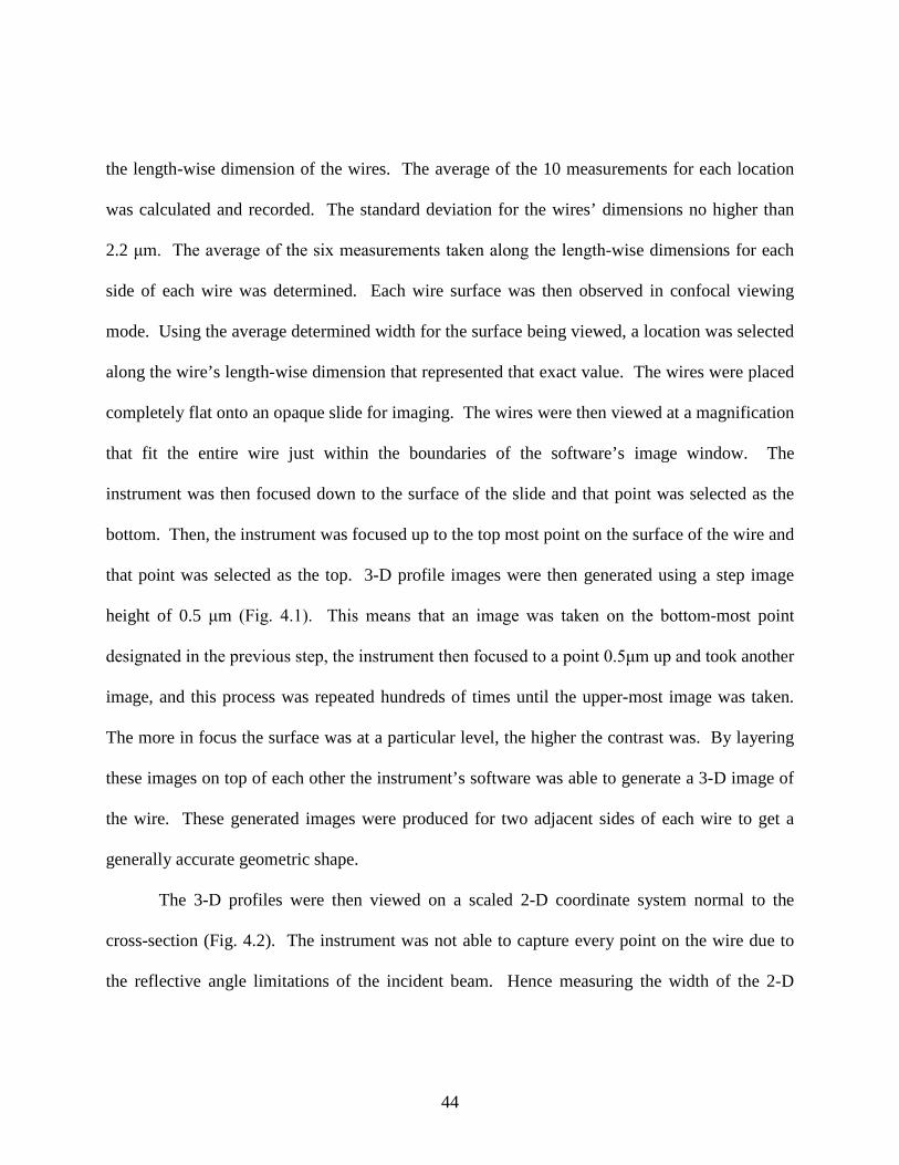
that point was selected as the top. 3-D profile images were then generated using a step image

height of 0.5 μm (Fig. 4.1). This means that an image was taken on the bottom-most point

designated in the previous step, the instrument then focused to a point 0.5μm up and took another

image, and this process was repeated hundreds of times until the upper-most image was taken.

The more in focus the surface was at a particular level, the higher the contrast was. By layering

these images on top of each other the instrument’s software was able to generate a 3-D image of

the wire. These generated images were produced for two adjacent sides of each wire to get a

generally accurate geometric shape.

The 3-D profiles were then viewed on a scaled 2-D coordinate system normal to the

cross-section (Fig. 4.2). The instrument was not able to capture every point on the wire due to

the reflective angle limitations of the incident beam. Hence measuring the width of the 2-D

45

representation and comparing it to the recorded value it was possible to verify that the outermost

points of the wire were captured. The images were then converted into a system of coordinates;

over 1,000 for each profile. The wire cross-sections were then redrawn and measured for their

cross-sectional area using SolidWorks®. After mechanical testing of calibration wires and

calculating the elastic modulus using the above method for cross-sectional area calculation, it

was shown to be an accurate method for determination of wire cross-sectional area.

In addition, a wire was mounted in epoxy, mechanically polished and etched, and the

surface analyzed using LSCM to determine the grain size for comparison to bulk samples

analyzed in previous work [Bigelow 2006].

Figure 4.1: Example 3-D profile image using Laser Scanning Confocal Microscopy

46

Figure 4.2: Example 2-D profile of cross-section after filtering out noise

4.4 Dynamic Mechanical Analysis

A dynamic mechanical analyzer (DMA) was used to determine the thermo-mechanical

properties of the NiTiPd wires. A DMA “supplies information about major transitions as well

as secondary and tertiary transitions not readily identifiable by other methods,” [Menard 1999].

For this reason a DMA was considered suitable for testing such thin SMA wires. The following

sections detail the components, operation and calibration of the DMA, as well as the thermo-

mechanical testing that was performed on the NiTiPd wires in the DMA after full calibration,

and in the process builds on work done by a previous author [Nandiraju 2006].

47

4.4.1 Equipment

The DMA setup consists of a cooling tank that, along with the cooling controller, helps

control the temperature inside the test section, a cooling cylinder that cools the internal

components of the DMA when operating at high temperatures, a computer-based software

package which controls the system, and the DMA itself (Fig. 4.3).

1. Perkin Elmer Diamond DMA

Equipment List:

2. Computer – MUSE Software

3. Furnace Cooling Tank

4. Furnace Cooling Controller

5. DMA Cooling Cylinder

Figure 4.3: DMA Equipment

48

4.4.1.1 Perkin Elmer Diamond DMA

The Diamond DMA can measure the rheological behavior of a material under dynamic

and static conditions, as a function of temperature, stress, time, frequency, or a combination of

these parameters. The Diamond DMA uses Fourier transform to reduce signal noise, thereby

being capable of detecting very weak transitions that may occur in the material during a

particular test. The system utilizes a heater that encompasses the test section for controlled

heating, an embedded LVDT which measures the probe displacement and a force generator to

provide a static or oscillatory (dynamic) force. The specifications of the DMA are outlined in

Table 4.1.

Table 4.1: DMA Specifications [Perkin Elmer]

49

4.4.1.2 Computer – MUSE Software

The MUSE software is the computer program which controls the total operation of the

DMA setup, and is user-controlled. The user can give inputs to the software to calibrate the

machine, as well as design the experiment and plot the resulting data.

4.4.1.3 Furnace Cooling Tank

The furnace cooling tank contains liquid nitrogen which is evaporated by a controlled,

internal heater and fed directly into the test section during operation and along with the internal

DMA heater can control the internal temperature of the test section between -150° to 600°C.

The supply line from the liquid valve of the tank must be screwed into the front of the DMA

furnace prior to testing, and the connection should be encapsulated using insulating material to

avoid losses. There are gauges on the tank which indicates the fluid level and the internal

pressure. The following instructions are to be used.

• Do not fill tank past 90% full to avoid over-pressurizing.

• Always have the gas release valve open during refilling of the tank.

• If pressure gauge on the cooling tank begins to rise, reduce flow of liquid nitrogen

from supply tank and open the release valve on the cooling tank more until pressure

stabilizes near 0 psi.

• Always use protective cryogenic gloves when filling tank.

• Do not move tank during use, whether it is being filled or feeding to the DMA.

50

4.4.1.4 Furnace Cooling Controller

The cooling controller links the user-controlled temperature program input to the MUSE

software to a control output valve on the furnace cooling tank which releases liquid nitrogen at

controlled rates to the DMA test section. The indicator lights on the controller tell the user, and

the system, how much liquid nitrogen is remaining in the tank (Fig. 4.4).

If the top indicator LED is lit then it is considered safe to operate the DMA for extended

periods of time (usually no more than 2-3 days). If the second LED is lit it is safe to run short

experiments (a few hours), but recommended to fill the tank a bit more before test. If the third

LED is lit the tank is at dangerously low levels and should be filled prior to use. If the bottom

light is lit the system will consider the liquid nitrogen levels unfit for use and not draw any liquid

nitrogen from the tank, regardless of the user writing a temperature program requiring controlled

cooling. Therefore, it is always recommended to refill the tank before programming any cooling

step in the experiment program which may exceed the levels available.

51

Figure 4.4: Furnace cooling controller showing fluid level indicator lights

4.4.1.5 DMA Cooling Cylinder

The cooling cylinder contains nitrogen gas and is a back-up measure that feeds into the

DMA inner components section. It is triggered automatically by the system when the test section

reaches a minimum of 400°C to ensure the DMA components do not overheat.

4.4.2 System Operation

This section explains how to turn on the DMA, replace the tension and bending fixtures,

load a sample, design and program an experiment, and properly turn off the DMA.

52

4.4.2.1 Turning on the DMA

1. Open the valve on the DMA cooling cylinder and adjust the release valve until the

pressure gauge reads between 45 – 55 psi.

2. Ensure the furnace cooling tank is full and plugged into the DMA furnace, and then

switch on the cooling controller.

3. Switch on the DMA power and wait for the display to read “LINKwait”.

4. Open the MUSE software application located on the computer and double-click on

the “measure” icon.

5. Go to “File” “Open Communication Port”; ensure “Com 1” is highlighted and

click “OK”.

6. The MUSE software will begin linking to the DMA; allow the DMA to display

“READY” before proceeding.

7. The MUSE software will display a message asking the user to initialize the system.

Before clicking to initialize, make sure there is no sample loaded in the test section

and that the probe is free to translate in the vertical direction when the force generator

is activated during initialization, i.e., nothing is contacting the probe that could

impede its movement. The user must take the following precautions.

• Do not put excessive force on the probe when removing samples or you

could damage the load-train.

• See Section 4.4.2.2 for directions on opening and closing the furnace.

• See Section 4.4.2.3 for directions on mounting and removing samples.

53

8. Click “OK” to initialize the system when the previous step is complete; make sure the

“Move to the target position” box is unchecked, and the “Adjust the offset load” box

is checked.

9. The system will take 1-2 minutes to initialize; the MUSE software will say “Ready”

in the upper left hand portion of the screen when done.

• The display on the DMA must read between ±5 μm, otherwise you must re-

initialize until that range is met.

10. At this point it is safe to load your test sample, begin writing the program and test.

• See Section 4.4.2.4 for procedure on writing the program.

4.4.2.2 Replacing the Fixtures

There are many different types of fixtures which can be used in the DMA; these include

bending, tension, shear, film shear, compression, and three-point bending. For the purposes of

this work only the tension and bending fixtures will be discussed. In order to replace the fixture

or mount a sample you must first switch on the DMA and allow it to display “LINKwait” before

opening the furnace. To open the furnace, see Figure 4.5. When opening the furnace, you must

wait until the furnace moves down and then all the way back before releasing the buttons. When

closing the furnace, you must wait until the furnace moves forward and then all the way up until

it seals with the DMA before releasing the buttons.

54

Figure 4.5: How to move the DMA furnace

4.4.2.2.1 Tension to Bending

First you must turn on the DMA in order to open the furnace. Keep the furnace fully

open and moved back into the recess before attempting to replace the fixture or you risk

dropping pieces into the test chamber.

1. Remove the (4) hex screws from the bottom of the base of the tension fixture that

are holding it to the protruding DMA pegs (Fig. 4.6).

2. Open the “Module” “Motor Control” box in the MUSE software and type in

“-16” as your “Target Position” and click “Move”.

55

3. When the position is reached, loosen the (2) probe screws from the probe and

remove the upper portion of the tension fixture (Fig. 4.6).

4. The bending fixture should already be assembled, and held together with a custom

plate gap setting provided by Perkin Elmer (Fig. 4.7).

5. Loosen the (2) probe screws on the bending fixture and affix the bending fixture

into position onto the bottom of the protruding DMA pegs and make sure the

plates being held together by the (2) probe screws are wrapped around the probe

tip (Fig. 4.8).

• Make sure the probe is resting naturally and not being forced in any

direction by the plates on the bending fixture being held together by

the (2) probe screws.

6. Lock the bending fixture into position with the (4) hex screws and then tighten the

(2) probe screws so the probe is secured to the bending fixtures top portion.

7. Loosen the (2) sample set screws all the way and remove the steel locking bar.

8. Open the “Module” “Motor Control” box in the MUSE software and click the

“Auto adjustment” button for the system to assess the new weight of the probe

attachment, and click the “Close” button when it has completed.

9. Initialize the system again to ensure accuracy, and the system is ready for testing

using the bending fixture.

56

Figure 4.6: Tension fixture assembled to the DMA

Figure 4.7: Fully assembled bending fixture

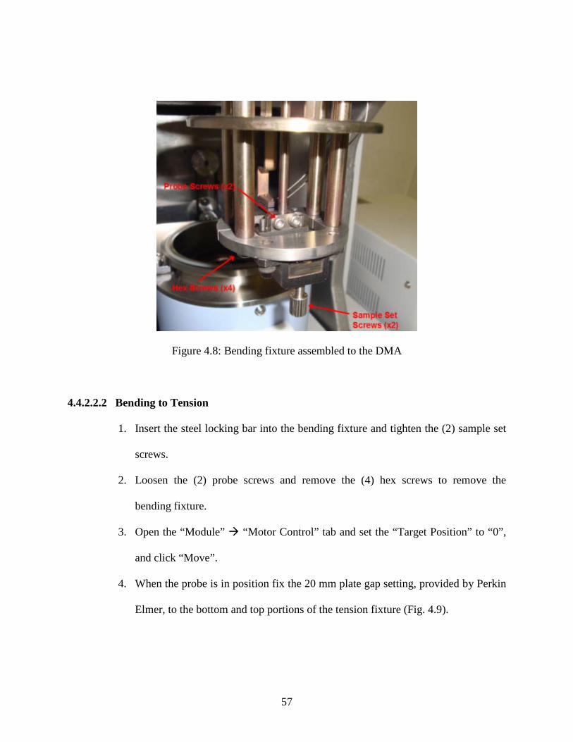
57

Figure 4.8: Bending fixture assembled to the DMA

4.4.2.2.2 Bending to Tension

1. Insert the steel locking bar into the bending fixture and tighten the (2) sample set

screws.

2. Loosen the (2) probe screws and remove the (4) hex screws to remove the

bending fixture.

3. Open the “Module” “Motor Control” tab and set the “Target Position” to “0”,

and click “Move”.

4. When the probe is in position fix the 20 mm plate gap setting, provided by Perkin

Elmer, to the bottom and top portions of the tension fixture (Fig. 4.9).

58

• Fix the spacer into position so both portions of the tension fixture are

flush against the insets of the 20 mm spacer to ensure accuracy.

5. Loosen the (2) probe screws and affix the tension fixture into position so the

DMA protrusions are recessed into the base of the tension fixture, and the plates

being held together on the upper portion of the tension fixture by the (2) probe

screws are enveloping the probe.

• Make sure the probe is resting naturally and not being forced in any

direction by the plates on the tension fixture being held together by

the (2) probe screws.

6. Tighten the (2) probe screws and remove the steel 20 mm spacer.

7. Re-tighten the tension fixture screws and use the “Auto adjustment” to reset the

new probe attachment weight.

59

Figure 4.9: 20 mm steel spacer for tension fixture

4.4.2.3 Loading the Sample

For the tension fixture:

1. Loosen the (2) top screws and the (2) bottom screws that are holding the set plates

together so there is a sufficient gap between the plates to insert your sample safely.

2. Hold the sample in position with a set of tweezers and re-tighten the (4) screws to

pin your sample between the top and bottom sets of plates.

• For more delicate samples it may be necessary to remove the front

plate of the bottom set to make sure you do not bend the sample when

positioning it into the tension fixture; replace the front plate of the

bottom set once the top set is tightened down and holding your sample

in position.

60

• Make sure the sample is long enough to extend at least 1 mm into the

voids between the plates pinching the sample, for both the bottom and

top set plates.

• Keep the probe as still as possible while positioning the sample.

• Do not over-tighten; once the screws are in tight enough to provide

some resistance you do not need to force it tighter. Doing so can

induce stress concentrations which may cause your sample to fail

prematurely during test/provide inaccurate data.

• The sample must be as vertical as you can get it, but not necessarily

centered. Although, it should be as centered as possible.

• You will notice the display on the DMA reading varying positions

while adjusting the sample. The display should read between ±25 μm

when the probe settles after you stop adjusting the sample. Otherwise,

you must loosen the grips and re-tighten until the probe is as relaxed

as possible, and the DMA display is reading between ±25 μm.

3. Close the furnace once the sample is fixed and the above conditions are met.

For the Bending Fixture:

1. Loosen the screws holding the horizontal set of probe plates together to allow

enough room to slide in the sample you are mounting.

61

2. Unscrew the (2) sample set screws all the way and slide your sample all the way

though the fixture so that it is resting midway between the probe attachment.

3. Tighten the (2) sample set screws all the way, then re-tighten the set of screws

loosed in step 1 to fix the sample completely.

• Make sure the sample is centered in the fixture and not at an angle.

4.4.2.4 Running an Experiment

Once the machine has been turned on, initialized, the sample has been loaded properly

and the furnace closed, you can begin programming the experiment.

1. On the MUSE software main screen open the “Conditions” “Condition Editor”

screen.

2. On the “Sample Condition” tab you must enter the sample name, shape and

dimensions, and then select the folder in which you want the program to save the

results, along with giving it a file name.

3. Open the “Method” tab, and select the type of measurement you would like to run.

a) SS control: Static tension mode.

b) Tension: Dynamic tension mode.

c) Bending: Dynamic bending mode.

• For the purposes of this work only SS control will be discussed further.

62

4. While staying in the “Sample Condition” tab, open the “Temperature Program”

tab and program in the temperature steps in which you would like the DMA to

follow.

a) Select the starting temperature in the first step to be the same upper

temperature read on the DMA display.

b) Enter the next temperature you would like to ramp to under the “Limit

(Cel)” column in the first step row.

c) Enter the rate at which you would like to increase or decrease the

temperature for the first step (between 0 - 20°C/min).

d) Enter the amount of time you would like the system to hold at that limit

temperature under the “Hold (min)” once the program temperature is

reached.

e) Fill in the additional temperature steps you would like to use for the

experiment, and check the end step you want the experiment to end with.

• Each step will begin at the exact time that the previous steps hold time has

ended.

• The program will end once the last temperature steps hold time has ended.

• It is necessary to enter higher than normal values for the temperatures in

your program because the resultant sample temperature will always settle

lower than the program temperature, i.e. if you want the sample to cycle

up to 250°C you must enter 269 as your program temperature. The higher

63

the temperature you program the larger the disparity between the actual

settled sample temperature and the program.

5. While staying in the “Sample Condition” tab, open the “SS Program” tab and

program in the loading steps in which you would like the DMA to follow.

• “F Control” will control force, and “L Control” will control displacement.

• “L control” will not work under certain material conditions.

6. Follow the same general procedure as you did for the temperature program.

7. After the temperature and load programs are set you can refer to the plot

displayed on the “Sample Condition” tab for a visual of the entire program to

ensure the temperature and loading steps match up correctly (Fig. 4.10).

8. Click “OK” on the bottom of the “Sample Condition” tab to open the MUSE

software profile screen.

9. Click the play button to begin the test, and then click on “View” “Profile”.

10. To customize the profile, double-click the axes to select the unit you would like to

follow, and with the axis highlighted you can expand or contract the range it

displays with the mouse wheel.

11. Once the program has ended you can analyze the results by going to the initial

MUSE software screen, and double-click the “Standard Analysis” button.

12. Open the file that you saved your experiment as and go to “File” “Output to

Excel,” for raw data.

64

13. If another experiment is to be run, you must remove the tested sample and reset

the motor control to the initial position before loading the next sample.

Figure 4.10: DMA experiment sequence plot viewed in MUSE software

4.4.2.5 Turning off the DMA

Whenever an experiment is not running, and you are going to be leaving the instrument

idle, you should turn off the DMA.

1. Remove any sample that may be mounted in the test section and re-tighten all

screws.

2. Close the furnace and go to “File” “Close Communication Port”. This will

power off the DMA and cooling controller.

3. Close the valves on the DMA cooling cylinder and close the MUSE software.

4.4.3 Calibrating the DMA

It is recommended to perform the full calibration procedure every 6 months. The

following procedures are arranged in the same order in which they need to be performed. Any

65

other order will result in a failed calibration, as the system recalculates certain constants after

each step is performed. As an exception, the temperature calibration can be performed anytime

with either the tension or bending fixture.

For the calibration procedure you will need the following testing materials:

1. PMMA (Poly-methyl Methacrylate) Plate (1.5 mm x 10 mm x 50 mm)

2. PMMA Plate (0.2 mm x 8 mm x 40 mm)

3. Stainless Steel Plate (3 mm x 10 mm x 50 mm)

4. Pure Iron Plate (0.4 mm x 10 mm x 50 mm)

5. Aluminum Plate (0.1 mm x 3 mm x 40 mm)

4.4.3.1 Temperature

The temperature calibration matches the recorded glass-transition temperature of PMMA

in the DMA to a reference value of 117°C.

1. Set the motor control position to “0 mm”, so the gage length becomes 20 mm.

Tension:

2. Open the “ABC Condition” tab and record the “0 order value”.

3. Measure the exact dimensions of the 0.2 mm thick PMMA sample and record in

the “Sample Condition” window, and then mount the PMMA sample (dimensions

0.2 mm x 8 mm x 40 mm) in the DMA.

66

4. In the “Temperature Program” select “Tension” as the mode, enter in a starting

temperature of 30°C and a limit temperature of 150°C for step one. Enter 2°C as

the heating rate, 0 min as the hold time, and 1 (s) as the sampling. Select step 1 as

the end step.

5. Select only 1 Hz as the DMS frequency.

6. Under DMS Tension Settings, select 10 μm as the L amp, 300 mN as the min.

tension/compression force, 1.5 as the tension/compression force gain, 4000 mN as

the force amplitude initial value, 10000 μm as the approved maximum

deformation, 8 (s) as the position movement wait time, and 0.0 sec/mN as the

creep wait time.

7. Run the experiment, and then open the plot in the standard analysis window.

8. Measure the peak temperature of the E” curve and using the equation (“New 0

order value” = a +117-b; where a = the initially recorded “0 order value”, and b =

the previously determined E” value), enter the “New 0 order value” into the ABC

condition window as the “0 order value”.

1. Load the bending fixture and mount the PMMA sample (dimensions 1.5 mm x

10 mm x 50 mm), making sure to record the exact dimensions into the

“Sample Condition” window.

Bending

2. Open the “ABC Condition” tab and record the “0 order value”.

67

3. In the “Temperature Program” select “Bending” as the mode and select

sinusoidal oscillation in the “DMS Frequency” tab. Enter in a starting

temperature of 30°C and a limit temperature of 150°C for step one. Enter 2°C

as the heating rate, 0 min as the hold time, and 1 (s) as the sampling. Select

step 1 as the end step.

4. Select only 1 Hz as the DMS frequency.

5. Run the experiment, and then open the plot in the standard analysis window.

6. Measure the peak temperature of the E” curve and using the equation (“New 0

order value” = a +117-b; where a = the initially recorded “0 order value”, and

b = the previously determined E” value), enter the “New 0 order value” into

the ABC condition window as the “0 order value”.

4.4.3.2 Compliance Correction

Before beginning the rest of the calibration, open the “DMS” tab under the “ABC

Condition” tab (Fig. 4.11), and enter the following values: set “F/L Gain” and “Tension Gain” to

“1”, set the “Load Span” to 11768, and set the remaining constants to “0”.

1. Load the bending fixture.

2. Measure and record the dimensions of the 3mm thick stainless steel plate into the

“Sample Condition” window.

3. Mount the 3 mm thick stainless steel plate into the bending fixture.

4. Open the “Method” tab and set the DMS mode to “Shear”.

68

5. Open the “Temperature” tab and set the control mode to “Step” mode, and set the

start temperature to “0”, the limit temperature to “10”, the step temperature to

“0.5”, and the soak time to 2 (s).

6. Open the “DMS Frequency” tab and select sinusoidal oscillation and 1 Hz as the

frequency.

7. Open the “DMS Tension Setting” and enter 20 μm as the L amplitude, 300 mN as

the force amplitude default, and click “OK” to complete the condition editor.

8. Click the “Test” button on the measurement screen, and when it is completed,

make sure the value falls with in the range on the screen. The “Test”

measurement initializes the DMS control system.

9. Click the play button to begin the actual measurement, and open the results using

standard analysis when it is completed.

10. Set the x-axis to “time”, and calculate the average value of G’

11. Open the “DMS” tab under the “ABC Condition” tab, and click the ellipses icon

next to the “Compliance Correction” box.

12. Enter the E’ value obtained in step 10 into the “Actual Calculation” box, and click

“OK”. If correct, the new calculated value in the Compliance Correction box

should read between 10-4 and 10-3

. Click “OK” to close the condition editor.

69

Figure 4.11: DMS calibration tab viewed in MUSE software

4.4.3.3 Time Constant Correction

1. Enter the exact measured dimensions of the 0.4 mm thick iron plate into the

condition editor.

2. Load the 0.4 mm thick iron plate into the bending fixture.

3. Check only the 100 Hz frequency under the “DMS Frequency” tab.

4. Keep all the remaining settings from the Compliance Correction procedure.

5. Click “OK” to close the “Condition Editor” window, and select “View”

“Profile” from the menu.

6. Open the “Axis Settings” from the tanD axis, make sure the “Logarithmic

Display” box is unchecked, and then click “OK”.

7. Click the “Test” button, and make sure the value falls within the range.

70

8. Click the play button and enlarge the tanD axis to view the maximized curve, and

record the average tanD value.

9. Open the “DMS” tab under the “ABC Condition”, and click on the ellipses next to

the “Time Constant” box.

10. Enter the recorded tanD value into the “Actual Measurement” box, enter “0.005”

in offset, 100 Hz in frequency, and then click “Apply” and “Close”.

11. If correct, the new calculated value should be on the order of 10-4

12. Click “OK”, and close the “Condition Editor” window.

.

13. Perform the measurement again and repeat the process until the tanD value has

dropped to 0.005 or lower.

4.4.3.4 Viscosity Correction

1. Remove any samples from the fixture.

2. Open the “DMS Frequency” tab and check only 20 Hz.

3. Open the “DMS Tension Condition”, and enter 10 mN for the force amplitude

default value, and then click “OK” to close the “Condition Editor” window.

4. Open the “Motor Control” window, and click “Auto Adjustment” for the offset

load. Click “Close”.

5. If the DMA display reads greater than the absolute value of 0.5 μm, initialize the

instrument before proceeding further.

6. Click the “Test” button on the measurement window, and then click “Close”.

71

7. Click the play button to run the sample-less experiment, and increase the tanD

range to 0 - 0.4.

8. Open the “DMS” tab under the “ABC Condition” tab, and enter a value between

0.5 – 2 for the viscosity correction.

9. Click “OK” and click play to measure the tanD range again.

10. Adjust the viscosity correction value in the “DMS” tab until the measured tanD

value falls within the range of 0.002 – 0.02. This can be seen by looking at the

results in standard analysis.

4.4.3.5 Probe Mass

1. No sample should be loaded for this calibration step.

2. In the dimensions section of the “Condition Editor”, Enter 0.01 mm for the

length, 1 mm for the width, and 5.1 mm for the thickness.

3. In the “DMS Frequency” tab, check only the 1, 10, and 20 Hz frequencies.

4. Click “OK” to exit the “Condition Editor”, and then click the “Test” button to

initialize the DMS control parameters.

5. Click the play button, go to “View” “Profile” on the measurement screen

while it’s testing and enlarge the G’ axis to bring the 3 frequencies just within

the screen.

72

6. Enter a value of 50 – 100 in the “Probe Mass” box under the “DMS” tab in the

“ABC Condition” section after each measurement until the conditions of step 7

are met.

7. The goal of this exercise is to have all 3 frequency responses as flat and parallel

as you can get it, and within 1 decade of each other. Adjust the “Probe Mass”

value until this condition is met. Will take several trial-and-error measurements.

4.4.3.6 Elasticity Correction

1. Open the “Standard Analysis” results of the final measurement from Section

4.4.3.5, and select the 1Hz curve for G’ from the drop-down menu on the results

screen. You should see brackets form around the curve of interest on the plot.

2. Read the value recorded for that curve (should be between 1000 – 3000).

3. Open the “DMS” tab under the “ABC Conditions” tab and enter in the value

recorded from step 2 into the “Elasticity Correction” box, and then click “OK” to

accept the changes to the “DMS” values.

4.4.3.7 F/L Gain

1. Record the exact dimensions of the 0.4 mm thick iron plate into the “Condition

Editor” main screen, and then load the 0.4 mm thick iron plate into the bending

fixture.

73

2. Open the “DMS Tension Setting” tab, and enter 2000 mN as the force amplitude

default value.

3. Make sure the DMS measurement mode is set to “Bending”, set the frequency

mode to “Sinusoidal Oscillation”, and check only the 1 Hz box under the “DMS

Frequency” tab.

4. Click “OK” to exit the “Condition Editor”, click the “Test” button to initialize the

settings, and make sure the elasticity ratio is displayed in the range.

5. Click the play button to begin testing, and then open the results in the “Standard

Analysis” when it has completed.

6. Set the x-axis to “Time”, and calculate the average E’ value.

7. Open the “DMS” tab under the “ABC Condition” tab, and click on the large box

marked with ellipses next to the “F/L Gain” box.

8. Enter 1.92E+11 as the E’ literature value, the value calculated from step 6 as the

actual measured E’, and then check the “F/L Gain”, “Viscosity Correction”,

“Probe Mass”, and “Elasticity Correction” boxes.

9. Click “Apply”, and then “Close”. The values in the left-hand boxes have now all

recalculated based on the value you entered for the “F/L Gain”.

10. Click “OK” to close the “Condition Editor” and accept the changes.

74

4.4.3.8 Tension Gain

1. Remove any sample that may be in the ending fixture and load the steel locking

bar and re-tighten all the screws, fixing the bar into position. This will hold the

entire bending fixture together.

2. Remove the bending fixture, reset the motor control to “0” to bring the gage

length to 20 mm, and then load the tension fixture. Make sure to use the “Auto

Adjustment” in the motor control tab to account for the new probe weight.

3. Initialize the instrument to bring the dL on the DMA display as close to “0”.

4. Record the exact measurements of the 0.1 mm thick aluminum sample in the

“Condition Editor”, and then load the 0.1 mm thick aluminum sample into the

tension fixture.

5. Open the “Condition Editor”, set the measurement mode to “Tension”, the

frequency mode to “Sinusoidal Oscillation”, and check only the 1 Hz box under

the “DMS Frequency” tab

6. Open the “DMS Tension Setting” tab, and enter 300 mN for the “Minimum

Tension/Compression”, 1.5 for the “Tension/Compression Gain”, 4000 mN for

the “Force Amplitude Default Value”, and then click “OK” to accept all changes.

7. Click the “Test” button to initialize the DMS control system.

8. Click the play button to run the measurement, and when it completes, open the

results under “Standard Analysis”.

9. Set the x-axis to time, and record the average E’ value.

75

10. Open the “DMS” tab under the “ABC Condition” tab, click on the ellipses next to

the “Tension Gain” box, record the literature value as 6.91E+10, and the actual

value as the E’ value calculated in step 9.

11. Click “Apply”, and then “Close” to save the changes.

12. Click the play button to run the measurement once more to ensure the new E’

value measured from the results is 6.91E+10 (±0.01E+10).

4.4.3.9 Load Sensitivity Correction of Static Control Mode

1. Remove any sample that may be loaded in the tension fixture.

2. Remove the base of the tension fixture so that only the upper portion is connected

to the probe.

3. Open the “Motor Control” window and perform an “Auto Adjustment”.

4. Initialize the DMA to bring the dL on the DMA display as close to “0”.

5. Open the “Method” tab under the “Condition Editor” window, select “SS

Control” mode, and under the “SS Control” tab put it in “L Composite” control.

6. Open the “ABC Condition” tab and enter 11768 mN for the load span, then click

“OK” to save and close the “Condition Editor” window.

7. Using a known 50 g weight, hang it from the upper portion of the tension fixture

that is attached to the probe using a string, which will add an insignificant amount

of weight.

76

• Make sure the weight is hanging directly below the probe, so there is no

moment generated.

8. Open the “Condition Editor”, and enter in the “Temperature Program”, in step 1, a

start and finish temperature of whatever the current temperature is in the furnace,

enter an arbitrary rate (ex. 10°C/min), a hold time of 10min, sampling of 1 (s),

and select step 1 as the end step.

9. For the “SS Program”, in step 1, enter 0 μm as the start and limit point, enter an

arbitrary rate (ex. 10 μm/min), and a hold time of 10 min.

10. Click “OK” to save the changes, and then click the play button to start the

measurement.

11. The DMA will adjust until the dL on the DMA display stabilizes at/near 0μm,

then record from the measurement screen of the MUSE software what the Force

output was at the moment the dL stabilized at 0 μm, and stop the measurement.

12. Open the “Condition Editor” window, then navigate to the “DMS” tab under the

“ABC Condition” tab and click on the ellipses next to the “Load Span” box.

13. Enter 490.333 mN as the literature value, and enter the measured force output

from step 11 as the actual value.

14. Click “Apply” to re-calculate the new load span, click “Close”, and then “OK” to

save all the changes.

77

4.4.4 Thermo-mechanical Testing of NiTiPd Wires

First, to verify the calibration procedure has adequately prepared the DMA for testing of

the fabricated NiTiPd wires, monotonic tensile tests were performed on materials of known

thermo-mechanical properties, as well as constrained recovery tests on a known commercial

HTSMA wire. Once the verification was complete, two different types of tests were performed

on the NiTiPd wires in the DMA; monotonic tensile tests and constrained recovery tests. These

tests can yield the most important thermo-mechanical data for a shape memory alloy that is being

developed for use in any actuator application. The data sets achieved during these tests will be

directly compared to thermo-mechanical results of the Ni29.5Ti50.5Pd20

bulk tension specimens

obtained in previous work [Bigelow 2006].

4.4.4.1 Calibration Verification

To ensure the DMA was functioning correctly and capable of providing valid, real

thermo-mechanical data, strain and temperature verification tests were performed on materials

with known thermo-mechanical properties after completion of the prescribed calibration

procedure detailed in Section 4.4.3. Room-temperature stress-strain tests were performed on

Steel, AlMgSi, and Superelastic NiTi wire to see if there was any additional compliance

correction to account for in SS Control mode. A commercial HTSMA wire was also tested in

constrained recovery to determine if the compliance correction made better agreement between

the literature response and the DMA response for the transformation strain. The commercial

HTSMA wire received had a diameter too large to test in the DMA under a 172 MPa hold stress,

78

which was the hold stress used in the reference curves for constrained recovery of that alloy.

Therefore, the wire was electropolished to bring down the diameter from 500 μm to 150 μm.

The transformation temperatures were also determined from the DMA response of the

commercial HTSMA wire and compared to the literature response to verify that the temperature

calibration was valid.

4.4.4.2 Monotonic Tensile Testing

Monotonic isothermal tensile tests were performed on “virgin” Ni29.5Ti50.5Pd20 wires with

rectangular cross-sections, with averaged dimensions of 150 ±2 μm x 130 ±2 μm for one set of

wires and averaged dimensions of 110 ±2 μm x 100 ±1 μm for a second set of wires. The grain

size for the wires was found to be equal to the grain size of the bulk samples (10 µm), which

makes about 200 grains to be present in the cross-section of the thicker wires, and about 100

grains present in the cross-section of the thinner wires. The reason for testing two sets of wires

with different cross-sectional areas was to evaluate any size-scale effects due to the number of

representative grains in the cross-section. Untested wires from each set were tested in the

martensitic and austenitic phase. For the martensitic phase tensile tests, untested samples from

both sets were loaded in the DMA at no-load and heated up to 73°C (Mf-50°) at a rate of

10°C/min and allowed to soak for a minimum of 15 minutes. Once equilibrium temperature was

established the samples were stressed at a rate of 250 mN/min up to a maximum of 5.8 N before

being unloaded at the same rate. For the austenitic phase tensile tests, untested samples from

both sets were loaded in the DMA at no-load and heated up to 193°C (Af+50°) at a rate of

79

10°C/min, through its phase transformation, and allowed to soak for at least 15 minutes. Once

equilibrium temperature was established the samples were stressed at a rate of 250 mN/min up to

a maximum of 5.8 N before being unloaded at the same rate. Tensile testing in the austenitic

phase was also carried out at 243°C (Af+100°) to determine if there could have been retained

martensite in the samples at Af+50°. The reference Mf and Af temperatures used for these tests

are presented in Section 5.3.2. The apparent yield stress for these responses were calculated and

compared to the previously reported bulk sample data [Bigelow 2006].

4.4.4.3 Constrained Recovery

Load-bias tests were performed on electropolished Ni29.5Ti50.5Pd20 wires using 20 mm as

the gage length and rectangular cross-sections with average overall dimensions of 150 ±2 μm x

130 ±2 μm. The cross-sectional shape of the electropolished wires was determined using profile

images taken using an Olympus LEXT OLS3000 Laser Scanning Confocal Microscope in

confocal viewing mode. The previous work which measured thermo-mechanical data from

NiTiPd bulk specimens had thermally cycled the bulk tension samples twice under no-load

conditions in a mechanical tester, but since the DMA had proven to respond inaccurately during

the cooling cycles at no-load it was safer to thermally cycle the wires in a furnace, rather than

subject them to conditions which may induce plasticity when none should be expected. Thermal

cycling can affect a shape memory alloy’s performance, therefore it was considered a necessary

step to thermally cycle them anyway to make sure they compared well to the bulk samples’

testing procedures. After thermal cycling in a furnace, the untested wires were loaded in the

80

DMA at no-load and heated up to 50°C at a rate of 10°C/min, which is well below the Mf

Figure 4.12 shows a schematic of how actuator-type performance data was extracted

from the constrained recovery curves for the micron-scale wires and bulk tensile sample

thermally cycled at incrementing stress levels. The transformation temperatures (As, Af, Ms,

and Mf) were measured from the second thermal cycle at each stress level using the intersection

of fit lines through the transformation and the linear coefficient of thermal expansion (CTE)

regions of the curves. The transformation strains (ε

established in previous work for bulk NiTiPd specimens [Bigelow 2006]. The samples were

then loaded up to 99 MPa at a rate of 250 mN/min and allowed to settle for about 5 minutes

before being heated up to 250°C at a rate of 2°C/min, and allowed to soak for 1 minute before

being cooled back down to 50°C at a rate of 2°C/min. After being allowed to soak at 50°C for 1

minute the sample was heated again in the same manner up to 250°C at 2°C/min and cooled back

down to 50°C at 2°C/min. The sample was then loaded isothermally up to 197 MPa at a rate of

250 mN/min and thermally cycled twice at this stress level in the same manner as was done

under the previous load. The sample was loaded isothermally up to 295 MPa in the same manner

and thermally cycled twice between 50°C and 250°C. The second thermal cycle at each stress

level is what was plotted and compared to the constrained recovery data from the previously

reported bulk sample data [Bigelow 2006].

TF) were measured as the difference between

the strains at the austenite finish and austenite start intersections, and the work output at each

stress level was calculated by multiplying the transformation strain by the applied stress. The

81

open-loop strain (εOL

), or irrecoverable strain, was measured as the strain difference between the

beginning of the heating curve and the end of the cooling curve.

Figure 4.12: Schematic showing data extracted from constrained recovery experiments

82

CHAPTER FIVE: RESULTS AND DISCUSSION

Following EDM of the bulk sample to produce rectangular cross-section wires on the

order of 200 μm in diameter, a heat-affected zone is formed on the new surfaces caused by the

rapid local heating and cooling from the pulse current which creates very high thermal gradients.

Successful removal of the entire HAZ from the samples was considered crucial to attaining

representative bulk thermo-mechanical responses from the wires to be tested in the DMA. For

this reason, EDM sample dimensions were made moderately larger than the desired final

electropolished wire dimensions. In going from an EDM sample with initial cross-section

dimensions of 210 μm x 200 μm to an electropolished sample with cross-section dimensions of

150 μm x 130 μm, and 110 μm x 100 µm, 6-10 minutes is required to remove material from the

wires to make them sufficiently small to go up to large stresses in the DMA. The time associated

with this process has been shown to increase surface roughness, although the finish surface

roughness of the wires was within the range established in previous work [Pohl et al. 2004].

After fabrication of the wires by wire-EDM and electropolishing, they were tested in a DMA for

their thermo-mechanical response and compared to previously reported results for a bulk tension

specimen similar to the one used for extraction of the wires [Bigelow 2006].

83

5.1 Effects of Electrical-Discharge Machining

After EDM, the wires were shown to have a rough surface from where the rapid re-

melting and solidification occurred (Fig. 5.1). Backscattered electron (BSE) images were taken

using SEM and Energy Dispersive X-ray Spectroscopy (EDX) of the surfaces was performed.

The results showed a combination of oxides and remelt on the wire’s surface (Fig. 5.2, 5.3). An

SEM image of a 3.2 mm section of the wire shows the wire to be uniform along its length (Fig.

5.4). TEM shows changes of the near-surface layer of the wires where oxides have now formed

due to the EDM process (Fig. 5.5). Another cross-section of the EDM wire was extracted by FIB

and a Scanning TEM (STEM) image obtained. The profile shows that the damage zone is rich

with oxide particles, but after a depth of 5 μm the sample is free of any damage from the EDM

process (Fig. 5.6).

Figure 5.1: SEM image of wire surface after EDM

84

Figure 5.2: EDX of oxides on wire surface after EDM

Figure 5.3: EDX of remelt on wire surface after EDM

85

Figure 5.4: Uniformity of wire after EDM

Figure 5.5: Formation of oxide particles near surface of wire after EDM

86

Figure 5.6: STEM image of wire cross-section after EDM and line EDX profile

87

5.2 Effects of Electropolishing

The wires produced by EDM were electropolished from their original dimensions of 210

μm x 200 μm down to no greater than 150 μm x 140 μm fo r any of th e DMA-tested wires

presented in this work. While the depth of the HAZ appeared to be no more than 5μm, the true

microstructural impact the EDM process could have had on the material could be slightly deeper.

To ensure the HAZ would be completely removed and not affect the thermo-mechanical

response of the wires when tested in the DMA, a minimum of 30 μm was removed from the

surface of each wire on each side.

The electropolished wires were observed in the SEM and shown to have a smooth surface

(Fig. 5.7). The samples also maintained uniformity throughout the electropolishing process (Fig.

5.8). However, some small particles presented themselves on the surfaces of the electropolished

wires, which are represented by the small contrast spots on the surface seen in Figure 5.7. STEM

confirms these particles are nearly pure titanium (Fig. 5.9). It is not clear from the literature why

the presence of these nearly pure titanium particles have formed on the surface as a result of

electropolishing. Figure 5.9 also shows that the expected Ti2

(Ni,Pd) phase was present

throughout the core of the wires, as they are the same ones present in the microstructure analysis

done in previous work on bulk NiTiPd specimens [Bigelow 2006]. TEM verifies that the HAZ

had been removed from both the 150 μm x 130 μm wires and the 110 μm x 100 μm wires, and

there was a fully martensite structure present at the surface (Fig. 5.10, 5.11).

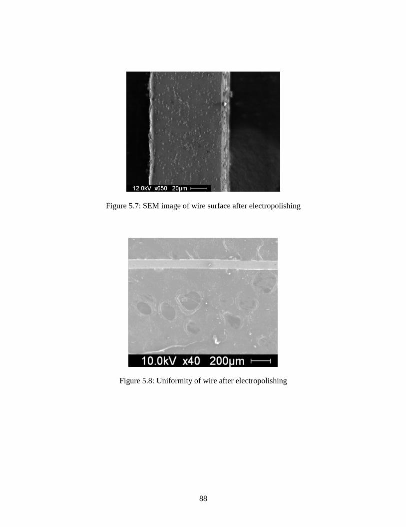
88

Figure 5.7: SEM image of wire surface after electropolishing

Figure 5.8: Uniformity of wire after electropolishing

89

Figure 5.9: STEM images from electropolished wire

90

Figure 5.10: TEM image of 150 μm x 130 μm wire showing absence of HAZ

Figure 5.11: TEM image of 110 μm x 100 μm wire showing absence of HAZ

1 µm1 µm

Surface

0.5 µm0.5 µm

Surface

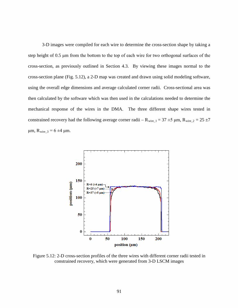
91

3-D images were compiled for each wire to determine the cross-section shape by taking a

step height of 0.5 μm from the bottom to the top of each wire for two orthogonal surfaces of the

cross-section, as previously outlined in Section 4.3. By viewing these images normal to the

cross-section plane (Fig. 5.12), a 2-D map was created and drawn using solid modeling software,

using the overall edge dimensions and average calculated corner radii. Cross-sectional area was

then calculated by the software which was then used in the calculations needed to determine the

mechanical response of the wires in the DMA. The three different shape wires tested in

constrained recovery had the following average corner radii – Rwire_1 = 37 ±5 μm, Rwire_2 = 25 ±7

μm, Rwire_3

= 6 ±4 μm.

Figure 5.12: 2-D cross-section profiles of the three wires with different corner radii tested in constrained recovery, which were generated from 3-D LSCM images

92

The surfaces of the electropolished wires were also viewed using LSCM in confocal

mode at a magnification of 2400x to determine surface roughness. The wire was imaged in 3-D

at a step height of 0.01 μm (Fig. 5.13). The root-mean square (RMS) surface roughness was

determined using the LSCM software to be 0.4 μm.

Figure 5.13: 3-D surface image of wire using LSCM after electropolishing

93

5.3 Thermo-mechanical Testing

To determine the thermo-mechanical response of the NiTiPd wires they were tested in a

DMA in SS Control mode using the tension fixture, as outlined in Section 4.4. The results of the

calibration verification, monotonic tensile testing, and constrained recovery testing are reported

in the following sections.

5.3.1 Verification of Instrument Calibration

The temperature calibration step described in Section 4.4.3.1 yielded accurate results for

the glass transition temperature of PMMA after calibration (Fig. 5.14). Monotonic tensile tests

were performed on stainless steel, Aluminum (98 at.% Al 1 at.% Mg and 0.6 at.% Si), and

superelastic NiTi wires to see if the Young’s modulus matched the reference values. After

loading each sample in tension mode and running a “Test” measurement in dynamic mode the

storage modulus (E’) of the material was established. The E’ values found using the “Test”

measurement method all fell within the reference value range for each of the tested alloys. After

recording the E’ of these three alloys, they were tested in the static “SS Control” mode, which is

the mode needed to determine actuator-type performance of the NiTiPd wires. Each alloy was

tested at room temperature, and stressed in force control at a rate of 250 mN/min up to a

predetermined stress that kept the material in the elastic region throughout the entire test (Fig.

5.15-5.17).

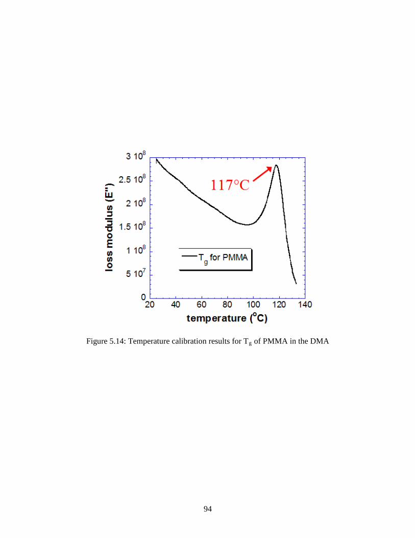
94

Figure 5.14: Temperature calibration results for Tg

of PMMA in the DMA

95

Figure 5.15: Stress-strain response of 127 μm diameter stainless steel wire in the DMA

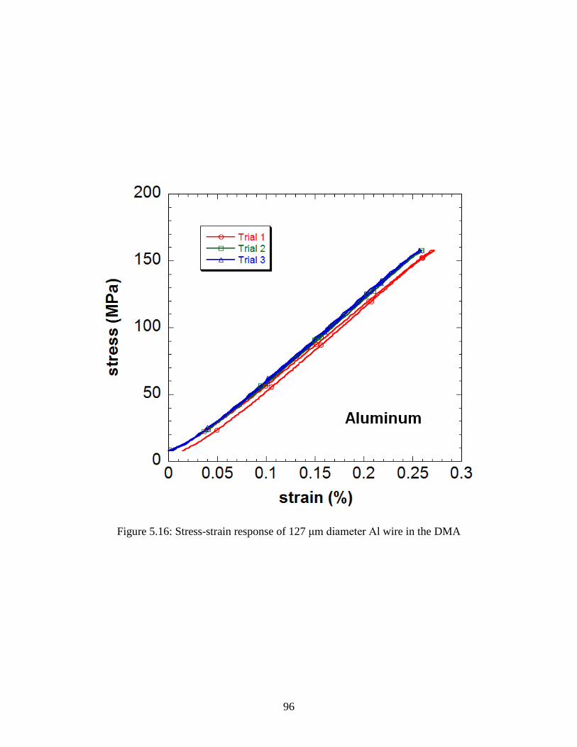
96

Figure 5.16: Stress-strain response of 127 μm diameter Al wire in the DMA

97

Figure 5.17: Stress-strain response of 178 μm diameter superelastic NiTi wire in the DMA

98

The calculated E/E’ ratios for each of the three alloys resulted in a 3:4 ratio (Table 5.1).

These results led to an additional instrument compliance that was factored into static tests

conducted in the DMA in “SS Control” mode.

Table 5.1: Comparison of moduli in DMA

Stainless Steel Aluminum Superelastic

NiTi

E' 200 GPa 83 GPa 79 GPa

E 150.7 GPa 62.7 GPa 59 GPa

E/E’ 0.7535 0.7554 0.7468

The electropolished commercial HTSMA wire was strained in force control up to 172

MPa at a rate of 250 mN/min at room temperature. After reaching the hold stress, the wire was

heated up to about 240°C at 2°C/min and then cooled down to about 40°C at 2°C/min. After

applying the instrument compliance determined in the beginning of this section, the DMA

constrained recovery response was plotted vs. the reference curve supplied with the wire (Fig.

5.18).

99

Figure 5.18: Comparison of constrained recovery of commercial HTSMA wire at a hold stress of 172 MPa (reference curves from manufacturer and the DMA response of the wire after

electropolishing to reduce size)

The transformation strain (εTF) of the reference HTSMA wire was 1.99%, whereas the

electropolished version of that wire in the DMA had a transformation strain of 1.69%. The As

for the wire was 4°C higher than that of the reference curves, the Af was 2°C lower, the Ms was

18°C lower, and the Mf was 10°C lower than the reference curves (Table 5.2). The differences

in the thermo-mechanical response are discussed later in the context of comparisons with the

bulk specimens. Regardless of the reason for the differences in the thermo-mechanical response

of the commercial HTSMA wire, a conclusion can be drawn that the DMA is properly calibrated,

100

and fully capable of assessing the actuator-type properties of a given shape memory alloy when

the additional instrument compliance is accounted for.

Table 5.2: Comparison of commercial HTSMA wire (reference values from manufacturer and DMA response of electropolished wire)

Mf M(°C)

s A(°C)

s A(°C)

f ε(°C)

TF Work

Output (J/cm(%) 3)

Reference 165 193 177 200 1.99 3.42

DMA 155 175 181 198 1.69 2.91

5.3.2 Monotonic Tensile Testing

Untested wires from both the 150 μm x 130 μm wire set and 110 μm x 100 μm wire set

were tested at 73oC and 193oC, which are Mf-50oC and Af+50oC, respectively. Those values

were established in previous work for the bulk samples of Ni29.5Ti50.5Pd20

Figure 5.19 shows the response of both the 150 μm x 130 μm wires and the 110 μm x 100

μm wires tested in the martensitic phase. The apparent elastic moduli of the two wires were

comparable, with the 150 μm x 130 μm wire having a modulus of 44 ±2.5 GPa, and the 110 μm

x 100 μm wire having a modulus of 38 ±2.5 GPa. The critical stress for detwinning was 131

MPa for the bulk sample, and 124 MPa and 112 MPa for the 150 µm x 130 µm and 110 µm x

100 µm wires, respectively.

[Bigelow 2006], and

the micron-scale wires were tested in the DMA at those same temperatures to ensure the alloy

was completely one phase of either martensite (B19) or austenite (B2).

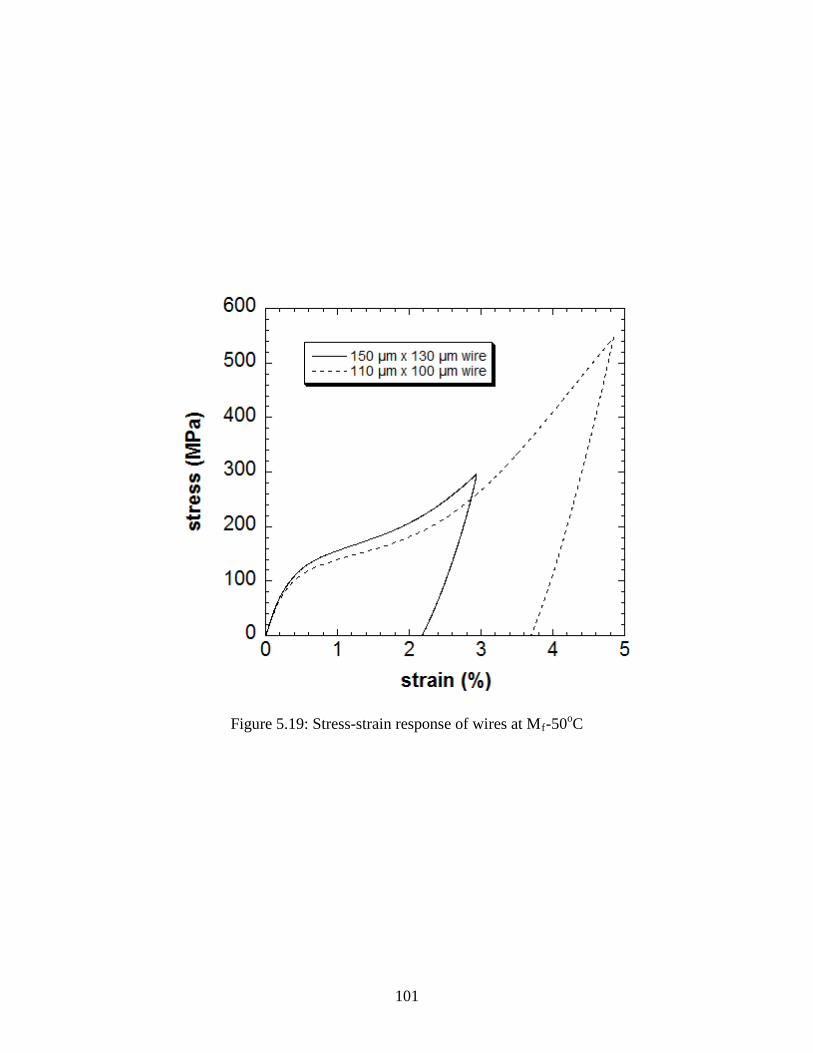
101

Figure 5.19: Stress-strain response of wires at Mf-50o

C

102

Figure 5.20 shows the response of both the 150 μm x 130 μm wires and the 110 μm x 100

μm wires tested in the austenitic phase. The elastic modulus for both wires was within error (72

±2.5 GPa, but given the DMAs force limitations, the 150 μm x 130 μm wire could not be loaded

to a stress high enough to induce plasticity. Therefore, the yield stress for the 150 μm x 130 μm

wire in its austenite state could not be determined.

Figure 5.20: Stress-strain response of wires at Af+50o

C

103

The modulus for the 150 μm x 130 μm wires were near equal between Af+50oC and

Af+100oC, with a modulus of 65 ±2.5 GPa, indicating that if retained martensite contributed to

the deflated modulus it is still stable at those higher temperatures (Fig. 5.21). The 110 μm x 100

μm wires also had similar elastic moduli, with a modulus of 62 ±2.5 GPa, but the yield stress of

the 110 μm x 100 μm wire tested at Af+100oC was higher than that of the one tested at Af+50oC

by 23 MPa, with the wire tested at Af+50oC yielding at 364 MPa and the wire tested at

Af+100o

C yielding at 387 MPa (Fig. 5.22).

Figure 5.21: Stress-strain response of 150 μm x 130 μm wires at Af+50oC and Af+100oC

104

Figure 5.22: Stress-strain response of 110 μm x 100 μm wires at Af+50oC and Af+100o

C

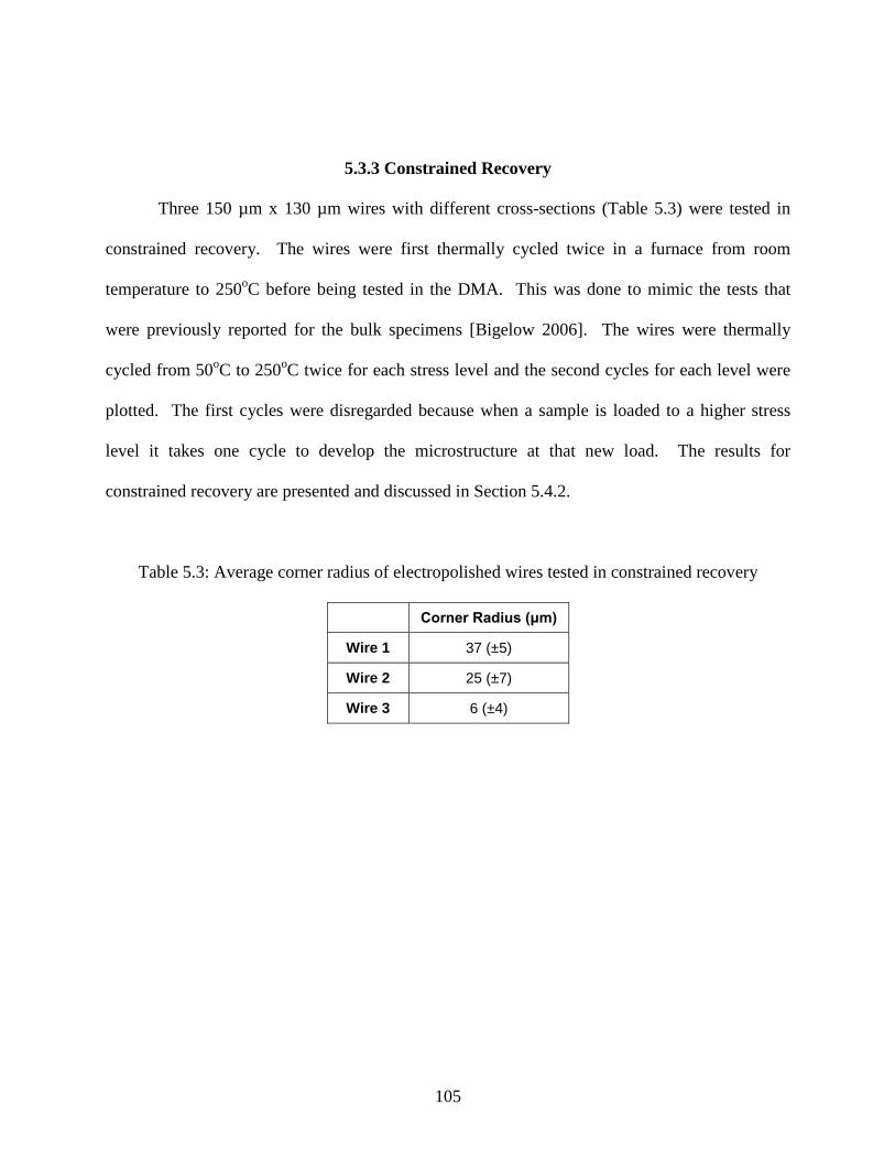
105

5.3.3 Constrained Recovery

Three 150 µm x 130 µm wires with different cross-sections (Table 5.3) were tested in

constrained recovery. The wires were first thermally cycled twice in a furnace from room

temperature to 250oC before being tested in the DMA. This was done to mimic the tests that

were previously reported for the bulk specimens [Bigelow 2006]. The wires were thermally

cycled from 50oC to 250o

C twice for each stress level and the second cycles for each level were

plotted. The first cycles were disregarded because when a sample is loaded to a higher stress

level it takes one cycle to develop the microstructure at that new load. The results for

constrained recovery are presented and discussed in Section 5.4.2.

Table 5.3: Average corner radius of electropolished wires tested in constrained recovery

Corner Radius (μm)

Wire 1 37 (±5)

Wire 2 25 (±7)

Wire 3 6 (±4)

106

5.4 Comparison of Micron-scale Wires to Bulk Tension Samples

After analyzing the thermo-mechanical responses of the NiTiPd wires in the DMA they

were compared to the bulk responses that had been previously reported [Bigelow 2006]. All of

the results for the NiTiPd bulk samples presented in this work are from previous work [Bigelow

2006], and were re-plotted from the original raw data for better visual comparison to the results

obtained in the DMA for NiTiPd wires of the same composition and bulk processing. The raw

data for the bulk samples were converted to engineering strain to match the engineering strain

plotted for the DMA results of the electropolished NiTiPd wires. For the purposes of direct

comparison the DMA wire results for constrained recovery have been offset to reflect the same

starting strains for each stress level as that of the bulk sample results. All of the results presented

in this section are directly responsible for the actuator-type performance of the alloy, and will

establish a confirmation that the DMA is a powerful tool for analyzing such properties.

5.4.1 Monotonic Tensile Testing

On comparing the martensitic stress-strain response of the two wires to the bulk sample,

it can be seen that the moduli are comparable, with the bulk sample having a modulus of 44 GPa

[Bigelow 2006], the 150 μm x 130 μm wire having a modulus of 44 ±2.5 GPa, and the 110 μm x

100 μm wire having a modulus of 38 ±2.5 GPa (Fig. 5.23).

107

Figure 5.23: Comparison of the stress-strain response of NiTiPd wires and the bulk sample; tested at Mf-50o

C

108

For the austenitic stress-strain responses, the wires displayed a slightly lower elastic

modulus of 72 ±2.5 GPa, as opposed to the 81 ±2.5 GPa for the bulk sample [Bigelow 2006],

possibly due to retained martensite in the samples, even at Af+50o

C (Fig. 5.24). The 110 μm x

100 μm wire was able to be loaded to the point of yielding, and was seen to plastically deform at

a lower stress than that of the bulk.

Figure 5.24: Comparison of the stress-strain response of NiTiPd wires and the bulk sample; tested at Af+50o

C

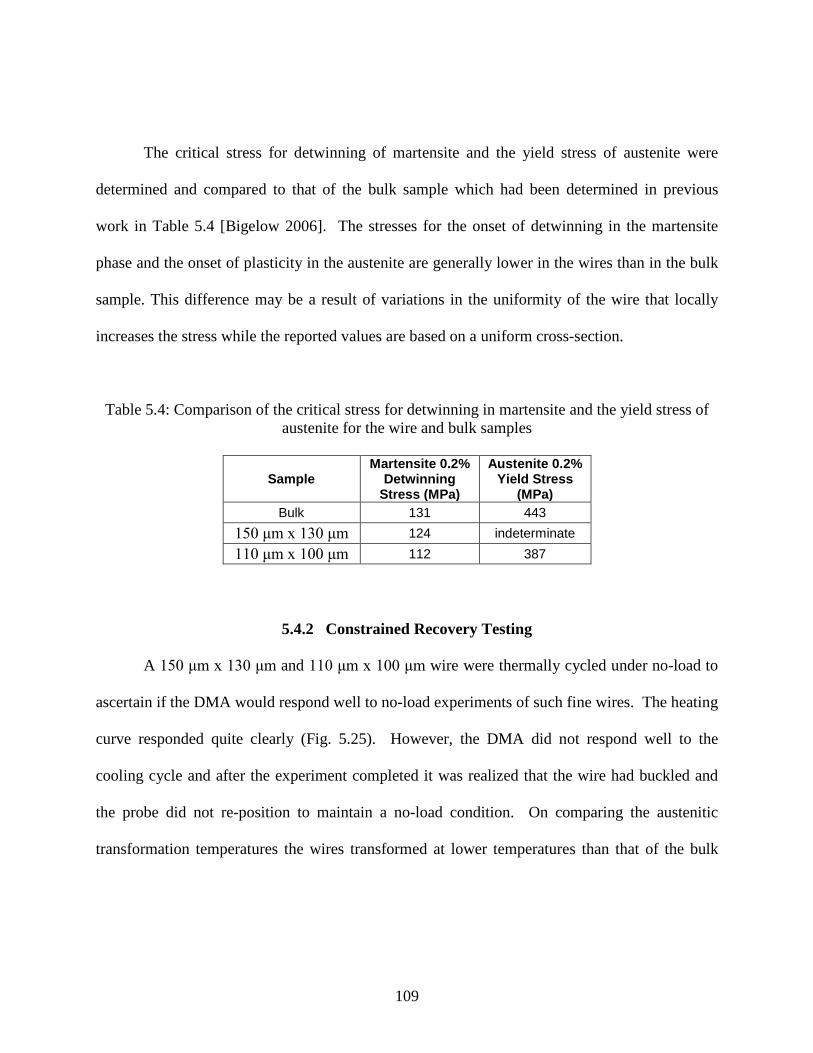
109

The critical stress for detwinning of martensite and the yield stress of austenite were

determined and compared to that of the bulk sample which had been determined in previous

work in Table 5.4 [Bigelow 2006]. The stresses for the onset of detwinning in the martensite

phase and the onset of plasticity in the austenite are generally lower in the wires than in the bulk

sample. This difference may be a result of variations in the uniformity of the wire that locally

increases the stress while the reported values are based on a uniform cross-section.

Table 5.4: Comparison of the critical stress for detwinning in martensite and the yield stress of austenite for the wire and bulk samples

Sample Martensite 0.2%

Detwinning Stress (MPa)

Austenite 0.2% Yield Stress

(MPa) Bulk 131 443

150 μm x 130 μm 124 indeterminate 110 μm x 100 μm 112 387

5.4.2 Constrained Recovery Testing

A 150 μm x 130 μm and 110 μm x 100 μm wire were thermally cycled under no-load to

ascertain if the DMA would respond well to no-load experiments of such fine wires. The heating

curve responded quite clearly (Fig. 5.25). However, the DMA did not respond well to the

cooling cycle and after the experiment completed it was realized that the wire had buckled and

the probe did not re-position to maintain a no-load condition. On comparing the austenitic

transformation temperatures the wires transformed at lower temperatures than that of the bulk

110

sample, but by no more than 12o

C (Table 5.5). For this reason the wires had been thermally

cycled twice in a furnace before being tested in the DMA under load.

Figure 5.25: No-load heating of wires

Table 5.5: Transformation temperatures acquired during heating

As (o AC) f (oC)

Bulk 133 143

150 μm x 130 μm Wire in DMA 125 131

110 μm x 100 μm Wire in DMA 125 134

111

At a hold stress of 99 MPa the wire with a cross-section that had a larger corner radius

than the others displayed a response most similar, in terms of transformation strain, to the bulk

sample which had a circular cross-section (Fig. 5.26). As the samples’ edges got sharper the

wire underwent less transformation strain as compared to the bulk sample. This can be attributed

to more geometrical constraints placed on the system in terms of the orientation of individual

variants for the case of sharper geometries. The transformation temperatures are lower in the

wires at the 99 MPa hold stress than that of the bulk sample. The difference in the

transformation temperatures can be attributed to intergranular stresses in the wire that affect the

transformation temperatures. At a hold stress of 197 MPa the wires displayed more closely

related values between each other for the transformation strains than for the 99 MPa hold stress

case (Fig. 5.27).

At higher applied stresses, the effects of intergranular stresses are overcome and hence

there is better agreement in the transformation temperatures between the wires and the bulk

sample. The effect of wire geometry is also reduced since the higher applied stresses more

strongly favor a certain distribution and orientation of variants. However, they did not display

the same relative amount of transformation strain compared to the bulk sample at this stress level.

The transformation temperatures of the wires were closer to that of the bulk sample for the 197

MPa hold stress case. At the final hold stress of 295 MPa the agreement between the wires’

transformation temperatures and strains were closer than in the previous cases (Fig. 5.28). The

difference between the transformation strains of the wires and the bulk sample were still present

at this higher stress level. The transformation strains between the wires get closer as the applied

112

hold stress is increased (Fig. 5.29). They are most comparable to the bulk at the lower stress;

however, get further from the bulk as stress is increased. In general at higher stresses there is an

inadequate number of grains (about 200 in the case of the 150 μm x 130 μm wires) to satisfy

stress and strain compatibility close to the wire surface while existing in an optimal distribution

and orientation of variants as in the bulk sample. The wires effectively display the same

irrecoverable strains as the bulk sample under each hold stress (Fig. 5.30). A summary of all the

above results is presented in Tables 5.6 and 5.7.

113

Figure 5.26: Comparison of constrained recovery response of wires and the bulk sample tested at 99 MPa

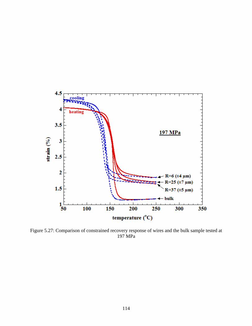
114

Figure 5.27: Comparison of constrained recovery response of wires and the bulk sample tested at 197 MPa

115

Figure 5.28: Comparison of constrained recovery response of wires and the bulk sample tested at 295 MPa

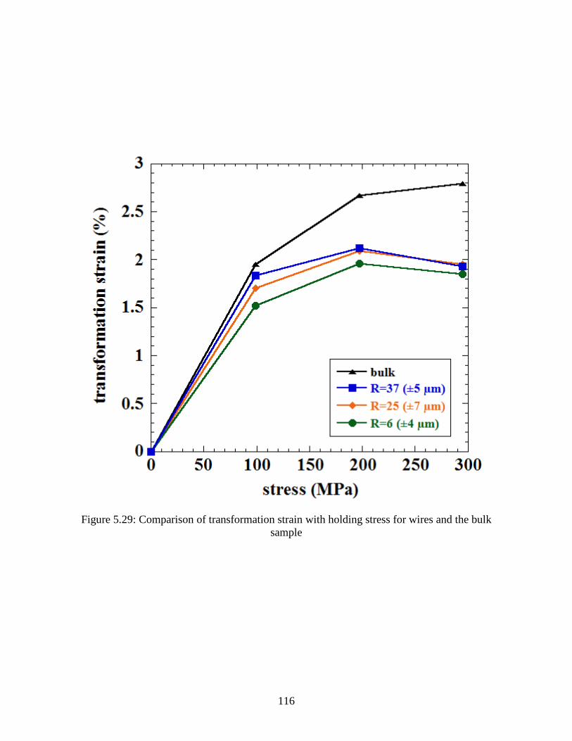
116

Figure 5.29: Comparison of transformation strain with holding stress for wires and the bulk sample

117

Figure 5.30: Comparison of irrecoverable strain with holding stress for wires and the bulk sample

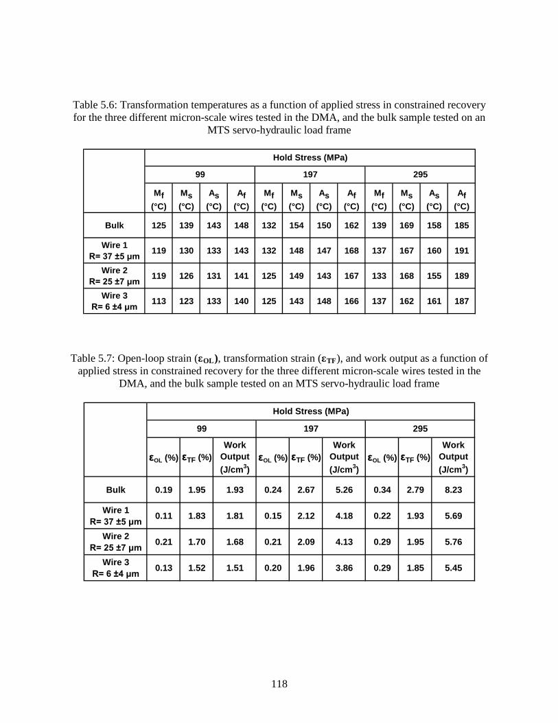
118

Table 5.6: Transformation temperatures as a function of applied stress in constrained recovery for the three different micron-scale wires tested in the DMA, and the bulk sample tested on an

MTS servo-hydraulic load frame

Mf (°C)

Ms (°C)

As (°C)

Af (°C)

Mf (°C)

Ms (°C)

As (°C)

Af (°C)

Mf (°C)

Ms (°C)

As (°C)

Af (°C)

Bulk 125 139 143 148 132 154 150 162 139 169 158 185

Wire 1 R= 37 ±5 μm 119 130 133 143 132 148 147 168 137 167 160 191

Wire 2 R= 25 ±7 μm 119 126 131 141 125 149 143 167 133 168 155 189

Wire 3 R= 6 ±4 μm 113 123 133 140 125 143 148 166 137 162 161 187

Hold Stress (MPa)

99 197 295

Table 5.7: Open-loop strain (εOL), transformation strain (εTF

), and work output as a function of applied stress in constrained recovery for the three different micron-scale wires tested in the

DMA, and the bulk sample tested on an MTS servo-hydraulic load frame

εOL (%) εTF (%)Work

Output (J/cm3)

εOL (%) εTF (%)Work

Output (J/cm3)

εOL (%) εTF (%)Work

Output (J/cm3)

Bulk 0.19 1.95 1.93 0.24 2.67 5.26 0.34 2.79 8.23

Wire 1 R= 37 ±5 μm 0.11 1.83 1.81 0.15 2.12 4.18 0.22 1.93 5.69

Wire 2 R= 25 ±7 μm 0.21 1.70 1.68 0.21 2.09 4.13 0.29 1.95 5.76

Wire 3 R= 6 ±4 μm 0.13 1.52 1.51 0.20 1.96 3.86 0.29 1.85 5.45

Hold Stress (MPa)

99 197 295

119

CHAPTER SIX: CONCEPT FOR A VARIABLE AREA LABYRINTH SEAL

Turbines are mostly designed around a “cold-build” clearance where the unstressed, room

temperature components are designed to have dimensions necessary to achieving minimum

clearance at equilibrium conditions during operation. Considering that the blades expand faster

than the shroud can accommodate, due to centrifugal forces, the shroud must be designed to be

slightly larger in radius. Otherwise, the blades will contact the shroud causing significant wear,

or even catastrophic failure. When the blades reach equilibrium the shroud continues expanding

due to thermal effects. This means the clearance gap at equilibrium conditions will be wider

than desired. By incorporating a labyrinth seal that is composed of shape memory actuators, a

final clearance can be controlled after startup, and not have to depend on a “cold-build”

clearance.

6.1 Background

Efficiency is a great concern with current turbine technologies. While it is desired to

have each stage in the turbine operating at optimum efficiency, the inlet compressor stages are

some of the most influential on the overall performance of a turbine. The inlet compressor

stages are also usually the least hot areas in a turbine’s flow-path area, and given the current

temperature limitations for shape memory alloys (SMA), is the most likely area to first apply

SMA actuators to aid in optimizing turbine efficiency. One of the biggest reasons for losses in a

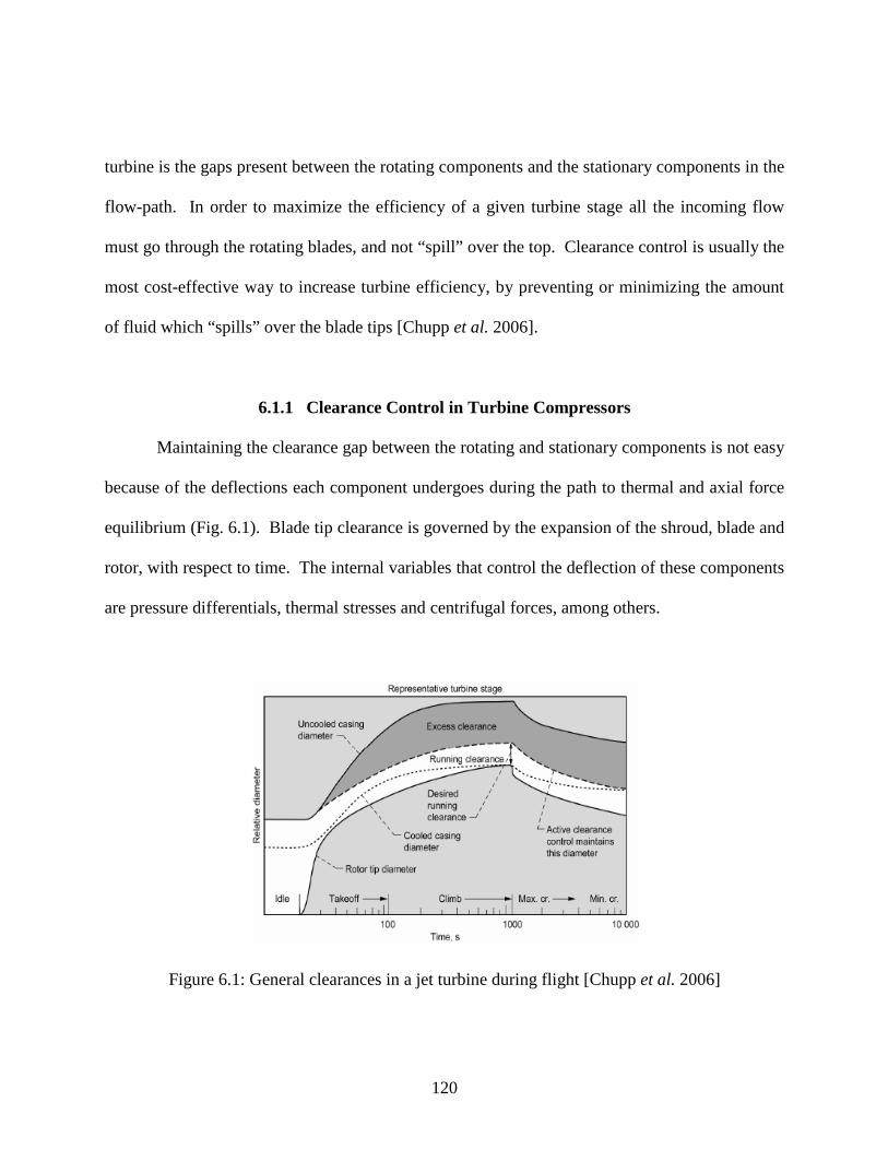
120

turbine is the gaps present between the rotating components and the stationary components in the

flow-path. In order to maximize the efficiency of a given turbine stage all the incoming flow

must go through the rotating blades, and not “spill” over the top. Clearance control is usually the

most cost-effective way to increase turbine efficiency, by preventing or minimizing the amount

of fluid which “spills” over the blade tips [Chupp et al. 2006].

6.1.1 Clearance Control in Turbine Compressors

Maintaining the clearance gap between the rotating and stationary components is not easy

because of the deflections each component undergoes during the path to thermal and axial force

equilibrium (Fig. 6.1). Blade tip clearance is governed by the expansion of the shroud, blade and

rotor, with respect to time. The internal variables that control the deflection of these components

are pressure differentials, thermal stresses and centrifugal forces, among others.

Figure 6.1: General clearances in a jet turbine during flight [Chupp et al. 2006]

121

Equation 6.1 is the general equation for an instantaneous tip clearance gap, where rshroud

is the inner wall position with respect to the center of rotation of the rotor, rrotor is the outside

surface position of the rotor with respect to its center of rotation and lblade

is the protrusion length

of the blade out from the outer surface of the rotor to its outer tip.

Clearance (t) = rshroud (t) – [rrotor (t) + lblade

(t)] (6.1)

The shroud radial deflection is governed by the pressure differential between the outer

and inner walls, and thermal stresses. The pressure differential effect on the shroud radial

deflection is dependent on the thickness of the shroud, the material properties of the shroud, the

mean internal pressure of the turbine at that location and the shroud external pressure. The

thermal stress effect on the shroud radial deflection is dependent on the thermal expansion of the

shroud material, the thickness of the shroud, and the temperature at the inner and outer wall of

the shroud.

The blade deflection is due to centrifugal forces and thermal stresses. The blade

deflection due to centrifugal forces is dependent on the material properties, the unstressed length,

and the angular speed of the blade. The blade deflection due to thermal stresses is dependant on

the coefficient of thermal expansion, the unstressed length and the mean temperature of the blade.

The rotor deflection is also due to centrifugal forces and thermal stresses. The rotor

deflection due to centrifugal forces is dependant on the material properties, the unstressed radius,

122

and the angular speed of the rotor. The rotor deflection due to thermal stresses is dependant on

the coefficient of thermal expansion, the unstressed radius and the mean temperature of the rotor.

By knowing the radial position profiles for each component in the system with time a

shape memory labyrinth seal can be designed to actuate with the timing necessary to avoid tip

contact with the seal, and to achieve and maintain a minimum clearance during steady-state

operation.

6.2 Proof-of-Concept

An ideal design would incorporate shape memory alloy segments positioned

circumferentially about a center point, and actuate to accommodate the gap change between the

“cold-build” radial position of the blade tip and the shroud. The SMA segments would need to

have biasing force acting on them in order to provide the necessary two-stage actuation.

Therefore, alloy segments of another material that does not have shape memory properties can be

circumferentially positioned about the center point and overlap the SMA segments. By

alternating the SMA segments with the biasing segments a seal can be made and two-stage

actuation can be achieved (Figure 6.2).

123

Figure 6.2: General design for proof-of-concept

6.2.1 Active vs. Passive Control

On starting the turbine, the blade tips expand rapidly and begin to come closer to the

labyrinth seal tips, which are circumferentially positioned on the inner surface of the shroud. A

minimum gap will be reached at a certain point, but the shroud will continue to expand at a faster

rate as a result of thermal expansion and widen the gap. This can be called the “pinch-point.” It

is at this pinch-point that the labyrinth seal tips will need to extend radially inward to close the

clearance gap.

The shape memory alloy segments can be actuated by either active or passive control.

Passive control would mean that the SMA segments would transform when the ambient

temperature causes it to do so. Once it reaches its austenite phase it would remain in that state

124

until the ambient temperature was reduced below the SMA’s Ms temperature. The SMA would

heat up by the hot flow inside the turbine and, when it reached its As temperature, it would begin

to transform into its stronger austenite phase, thereby pushing against the biasing segments and

changing the radial tip position of the labyrinth seal. Active control would mean that the SMA

segments would be heated externally by a controlled heating source, i.e., electrical induction

heating. The SMA can be actuated to position the seal at a higher radial position during startup

by intrinsically heating the SMA to above its Af temperature. Then, when the pinch-point is

reached, the heating can be stopped and the SMA allowed to cool to the flow-path temperature,

which would be less than the Mf

temperature for the alloy. This means that the system will

actually be active for a period of time, but transition to passive control once the induction heating

is stopped. For a visualization of the transformation path the SMA will take during either

passive or active/passive control for this application, see Figure 6.3.

125

Figure 6.3: SMA phase path for both passive and active/passive control

6.2.2 Actuation Methods

There are several different ways in which the various SMA and bias segments can be

positioned to provide two-stage actuation (Fig. 6.4). One method of actuation can involve the

overlapping of bias segments with SMA strips fixed to the back ends, or between the overlap

points. Another method can involve alternating overlapping SMA and bias segments. A

combination of these ideas is also possible.

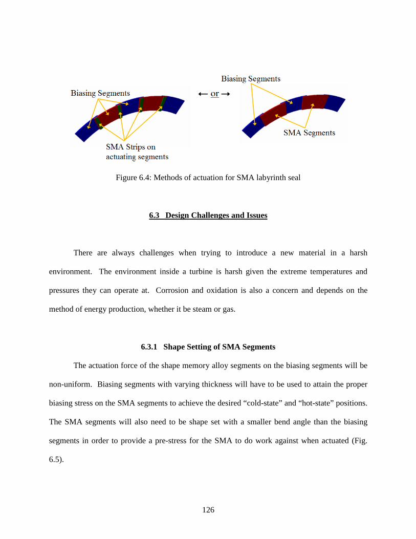
126

Figure 6.4: Methods of actuation for SMA labyrinth seal

6.3 Design Challenges and Issues

There are always challenges when trying to introduce a new material in a harsh

environment. The environment inside a turbine is harsh given the extreme temperatures and

pressures they can operate at. Corrosion and oxidation is also a concern and depends on the

method of energy production, whether it be steam or gas.

6.3.1 Shape Setting of SMA Segments

The actuation force of the shape memory alloy segments on the biasing segments will be

non-uniform. Biasing segments with varying thickness will have to be used to attain the proper

biasing stress on the SMA segments to achieve the desired “cold-state” and “hot-state” positions.

The SMA segments will also need to be shape set with a smaller bend angle than the biasing

segments in order to provide a pre-stress for the SMA to do work against when actuated (Fig.

6.5).

127

Figure 6.5: Method for producing desired pre-stress for SMA segments

6.3.2 Sealing between Segments

Given that the total radial displacement of the labyrinth seal tips should not need to

exceed about 1.25 mm the total deflection of the labyrinth seal about its center of curvature will

need to be on the order of 1°, depending on the height of the segments. The overlapping of the

segments in the array will provide a natural mechanical seal to prevent any flow between the

segments. The edges of the SMA segments will create a line contact with the contacting plane of

the biasing segments and would slide during actuation. This would mean that the assembly

would have to be impervious to flutter that may occur from the incoming flow. If the flow

creates any kind of minimal gap between the overlapping segments it is possible for a boundary

layer to form in the gap and hold the segments apart. Therefore, the rear segments of the

assembly need to have a higher stiffness than the front segments, so that the more compliant

segments will impact the stiffer rear segments during high-velocity flow, thus creating a better

mechanical seal and preventing flutter. For the active/passive design, the SMA segments need to

be placed in front of the biasing segments. Since the SMA segments will be in the martensitic

128

phase during steady-state operation it will be more compliant than the rear biasing segments.

Martensitic NiTi-based alloys also have excellent damping capabilities, meaning the spring-back

of the rear biasing segments will be greater than that of the SMA segments, thus maintaining a

mechanical seal even during any possible flutter.

6.3.3 Temperature Limitations

Certain areas of a turbine can reach temperatures of over 1000°C, and since most current

applications of shape memory alloys do not exceed 100°C further alloy development must be

done. The compressor stages of several ground-based turbines usually do not exceed 450°C.

Therefore, developing a shape memory alloy that can meet or exceed 450°C would go a long

way towards integrating them into a turbine. The methodology established in this work is

expected to aid in the quick and cheap development of a suitable shape memory alloy for use at

high temperatures. At the time of writing, NiTiPt alloys show promise for use at high

temperatures.

6.3.4 Cyclic Degradation

One of the main goals for turbine technologies is to have components that do not have to

be serviced or replaced for at least 2-5 years. In order for a shape memory alloy labyrinth seal to

be implemented it must also satisfy this criterion. Since the SMA segments do not undergo

much deformation their cyclic performance can be expected to be favorable when actuated, and

should not accumulate any plastic strain. NiTi has been able to perform for millions of cycles

129

after training when having to recover low strains and hence it is conceivable that new shape

memory alloys will perform similarly.

6.3.5 Heat Transfer

As previously explained in section 6.2.1, active or passive control relies on the

transformation temperatures of the alloy being used. It is essential that the labyrinth seal

segments not contact the blade tips, so accurate design and implementation is vital to a viable

SMA labyrinth seal. For passive control, the gas flow temperature will decide when the SMA

segments will begin actuation, so the actuation speed of the labyrinth seal must not be too fast or

it will contact the blade tips before steady-state is reached. Therefore, intimate knowledge of the

heat transfer in the entire system that would affect the temperature profile of the SMA segments

must be known, and accounted for in the design. For the active/passive control method, the

SMA will be held at an open position for the entire startup and through the pinch-point, but

knowing when to release it and allow for it to cool to the ambient flow temperature requires

intimate knowledge of the heat transfer as well.

6.3.6 Corrosion and Oxidation

While NiTi has been extensively studied for its corrosion and oxidation resistance the

HTSMAs being developed across the world have not been put under such rigorous testing for

such properties yet. Electropolishing NiTi to create a thin layer of TiO2 or coating it with a

barrier layer is quite common for current applications, but turbine environments are much more

130

hostile than the current environments SMAs are used in. Considering that NiTi begins a rather

rapid growth of oxidation above 600°C it is likely that some sort of special coating or isolation

of the SMA components altogether might be necessary to apply SMA inside harsh turbine

environments in the future.

131

CHAPTER 7: CONCLUSIONS

Micron-scale wires were extracted by wire electrical-discharge machining (EDM) from a

Ni29.5Ti50.5Pd20 bulk tensile specimen, and were subsequently electropolished to remove the

heat-affected zone (HAZ) from the surfaces of the wires, and to reduce the cross-section

dimensions for adequate thermo-mechanical testing in a dynamic mechanical analyzer (DMA).

The results of these thermo-mechanical tests were compared to previous results acquired from

corresponding Ni29.5Ti50.5Pd20

For purposes of direct comparison, electrical discharge machining (EDM) was used to

extract wires from the bulk samples. Characterization of the wires’ heat affected zone (HAZ)

was undertaken using scanning electron microscopy (SEM) and transmission electron

microscopy (TEM). TEM studies of the wires after EDM identified the depth affected by the

EDM process and hence the layer that needed to be removed to produce test samples capable of

exhibiting thermo-mechanical data representative of the core material. Electropolishing with

methanolic sulfuric acid was chosen as the method to remove the HAZ from the wires and

selecting the right electrolyte composition for electropolishing Ni

bulk tensile specimens at NASA Glenn Research Center.

29.5Ti50.5Pd20 needed to be

established. By varying the electropolisher parameters, i.e., input voltage and time, a process

was established for removing the HAZ from the surfaces of the wires, while maintaining

uniformity in the cross-section over the length of the sample. In addition, by varying the input

voltage between the established electropolishing voltage (6-8 volts) the corner radius of the

wires’ cross-sections were controlled to be different from one another.

132

Precise measurement of the wires’ cross-section area was required for determination of

the mechanical properties from DMA testing. Given the small cross-section of the wires tested

(of the order of 100 μm) and the delicate handling necessary for such wires it was difficult to

calculate the area of the wire cross-sections by non-destructive means. Therefore, a

methodology was established to measure the wire cross-section dimensions by using laser

scanning confocal microscopy (LSCM) in 3-D confocal viewing mode. This method not only

allowed for precise area measurement of the wires’ cross-sections, but provided the tools

necessary to measure the corner radius of these wires’ cross-sections as well.

Once valid test samples were produced a DMA was used to characterize the thermo-

mechanical properties of the Ni29.5Ti50.5Pd20 wires. Aside from the prescribed DMA calibration

procedure provided by the manufacturer, Perkin Elmer, additional instrument compliance was

needed based on monotonic tensile test results of stainless steel, aluminum and superelastic NiTi

wires. Constrained recovery tests at increasing stress levels of 99, 197 and 295 MPa were then

performed on micron-scale wires with overall dimensions of 150 μm x 130 μm (though they had

varying corner radii to represent different cross-section shapes); with wires having an average

corner radii of 37 μm, 25 μm and 6 μm, respectively. Isothermal tensile tests were also

performed on two different sets of micron-scale Ni29.5Ti50.5Pd20 wires in a DMA, at temperatures

of 73°C (Mf-50°C) and 193°C (Af+50°C) to ensure fully martensitic and fully austenitic

structures, respectively; with one set having overall cross-section dimensions of 150 μm x 130

μm, and the other set having overall cross-section dimensions of 110 μm x 100 μm.

133

On comparing the results from NASA’s previous testing on bulk tensile specimens with

that of the micron-scale wires, the overall thermo-mechanical trends were accurately captured by

the micron-scale wires for both the constrained recovery, and monotonic tensile tests.

Specifically, there was excellent agreement between the stress-strain response in both the

martensitic and austenitic phase, the transformation strains at lower stresses in constrained

recovery, and the transformation temperatures at higher stresses in constrained recovery. The

transformation strains were sensitive to the corner radius of the wires at lower stresses in

constrained recovery, and then became outweighed at higher stresses by the representative

number of grains in the cross-section.

Shape memory alloys (SMAs) have been used in many aerospace and aeronautical

applications, but have yet to be implemented in turbomachinery because both ground-based and

jet turbines have internal operation temperatures that far exceed the operational limit of any

commercially available SMA. Other factors, such as high pressures, vibrations, and creep effects

from rotating components, could also affect the behavior of SMAs. While it is desired to have

each stage in the turbine operating at optimum efficiency, the inlet compressor stages are some

of the most influential on the overall performance of a turbine. The inlet compressor stages are

also usually the least hot areas in a turbine’s flow-path area, thus are the most likely area to first

apply SMA-based actuators to aid in optimizing turbine efficiency. One of the ways to make a

compressor stage more efficient is to reduce the gap between the compressor blade tip and the

shroud. By allowing more area between the blade tips and the shroud less volume of gas will be

compressed, thus negating the purpose of the compressor stage. Complex seals are used in

134

turbomachinery to minimize “spillage” over turbine blades, but the main drawback to those seals

is they are made of rigid components which only change shape due to their respective coefficient

of thermal expansion. This work additionally has presented a concept for a variable area

labyrinth seal which uses high-temperature shape memory alloys (HTSMAs) to further reduce

the gap between the compressor blade tips and the shroud.

In order for NiTi-based SMAs to be implemented in high-temperature environments

elemental additions and special heat treatments must be used. Expensive elements, like platinum

and palladium, are encouraging ternary additions that raise the transformation temperatures of

NiTi. Melting large billets and machining tensile samples is expensive when trying to optimize

the thermo-mechanical properties necessary for a given application. By melting smaller buttons

and using a process that comprises both wire-EDM and electropolishing to produce thin wires,

the thermo-mechanical trends can be realized in a DMA, and be considered representative of a

bulk specimen. Once an optimized response is acquired, large-scale billets can be produced, and

bulk samples extracted from those billets can be used to further evaluate the material, e.g.,

dimensional stability, creep, etc. By improving upon the methodology presented in this work

through optimization of the EDM and electropolishing parameters, a more quantitatively similar

set of thermo-mechanical data to a bulk specimen can be expected.

The results of the experiments on Ni29.5Ti50.5Pd20 described in this work are very

encouraging and can potentially bring down the cost of shape memory alloy development in the

future. In driving down the costs associated with HTSMA development, less-expensive and

vigorous alloy development can commence which could accelerate the advancement of shape

135

memory alloy use in high-temperature environments. With the costs of electricity generation for

consumer use continually increasing and jet fuel costs poised to rise in the near future and

beyond, achieving greater turbine efficiency sooner, rather than later, can help to offset these

costs in the near-term. It is expected that the work presented in this thesis can help bring the use

of HTSMAs in turbomachinery closer to reality.

136

REFERENCES

Berg B., “Mechanics of NiTi Fatigue for Vascular Stent Design”, Society of Engineering Science:

45th

Annual Technical Meeting (2008).

Bigelow G., “Effects of Palladium Content, Quaternary Alloying, and Thermomechanical Processing on the Behavior of Ni-Ti-Pd Shape Memory Alloys for Actuator Applications”, NASA/TM – 2008-214702 (2008).

Bigelow G. S., Thesis, “Effects of Palladium Content, Quaternary Alloying, and

Thermomechanical Processing on the Behavior of Ni-Ti-Pd Shape Memory Alloys for Actuator Applications”, Colorado School of Mines, 2006.

Calkins F. T., Mabe J. H., Butler G. W., “Boeing’s Variable Geometry Chevron: Morphing

Aerospace Structures for Jet Noise Reduction”, Proc. of SPIE Vol. 6171 (2006). Carpenter B. F., Head R. J., Gehling R., “Shape Memory Actuated Gimbal”, Proc. of SPIE Vol. 2447 (1995), pp. 91-101. Chupp R. E., Hendricks R. C., Lattime S. B., Steinetz B. M., “Sealing in Turbomachinery”,

NASA/TM – 2006-214341 (2006). DeCastro J. A., Melcher K. J., Noebe R. D., “System-Level Design of a Shape Memory Alloy

Actuator for Active Clearance Control in the High-Pressure Turbine”, NASA/TM – 2005-213834 (2005).

Diakunchak I. S., U.S. Patent 6,926,495 (2005). Duerig T., Pelton A., Stöckel D., “An Overview of Nitinol Medical Applications”, Materials

Science and Engineering A, Vols. 273-275, (1999), pp. 149-160. Dunne J. P., Hopkins M. A., Baumann E. W., Pitt D. M., White E. V., “Overview of the

SAMPSON Smart Inlet”, Proc. of SPIE Vol. 3674 (1999), pp. 380-390. Dynalloy, Inc., Costa Mesa, CA, http://www.dynalloy.com/pdfs/TCF1140RevD.pdf Elliott R. S., Shaw J. A., Triantafyllidis N., “Stability of Thermally-Induced Martensitic

Transformations in Bi-Atomic Crystals”, Journal of the Mechanics and Physics of Solids, Vol. 50, (2002), pp. 2463-2493.

137

Elorriaga J., U.S. Patent 6,102,307 (2000). ESMA, Inc., South Holland, IL, http://www.esmainc.com/products/pdf/electropolishing/e1085-

1s.pdf Evans D. H., U.S. Patent 5,203,673 (1992). Funakubo H., “Shape Memory Alloys”, Gordon and Breach Science Publishers, New York, 1987. Fushimi K., Stratmann M., Hassel A. W., “Electropolishing of NiTi Shape Memory Alloys in

Methanolic H2SO4

”, Electrochimica Acta, Vol. 52, (2006), pp. 1290-1295.

Golberg D., Xu Y., Murakami Y., Morito S., Otsuka K., “Characteristics of Ti50Pd30Ni20

High-Temperature Shape Memory Alloy”, Intermetallics, Vol. 3, (1995), pp. 35-46.

Hsieh S. F., Chen S. L., Lin H. C., Lin M. H., Chiou S. Y., “The Machining Characteristics and Shape Recovery Ability of Ti-Ni-X (X = Zr, Cr) Ternary Shape Memory Alloys Using the Wire Electro-Discharge Machining”, International Journal of Machine Tools & Manufacture, Vol. 49, (2009), pp. 509-514.

Huang X. and Liu Y., “Effect of Annealing on the Transformation Behavior and Superelasticity

of NiTi Shape Memory Alloy”, Scripta Materialia, Vol. 45, (2001), pp. 153-160. Humbeeck J. V., “Non-Medical Applications of Shape Memory Alloys”, Materials Science and

Engineering A, Vols. 273-275, (1999), pp. 134-148. James V. L., U.S. Patent 4,196,856 (1980). Kim J. I., Liu Y., Miyazaki S., “Ageing-Induced Two-Stage R-Phase Transformation in Ti –

50.9at.%Ni”, Acta Materialia, Vol. 52, (2004), pp. 487-499. Lam S., Schoenwald K. D., Snyder D. W., Watson D. S., “Detailed Design Report for a Debris Free Control Release Mechanism Utilizing NiTi Shape Memory Alloys for the National Aeronautics and Space Administration”, Senior Design Project – University of Central Florida (Spring 2007). Lattime S. B., Steinetz B. M., “Turbine Engine Clearance Control Systems: Current Practices

and Future Directions”, NASA/TM – 2002-211794 (2002). Lattime S. B., Steinetz B. M., Robbie M. G., “Test Rig for Evaluating Active Turbine Blade Tip

Clearance Control Concepts”, NASA/TM – 2003-212533 (2003).

138

Lin B., Gall K., Maier H. J., Waldron R., “Structure and Thermomechanical Behavior of NiTiPt Shape Memory Alloy Wires”, Acta Biomaterialia, Vol. 5, (2009), pp. 257-267.

Lin H. C., Lin K. M., Cheng I. S., “The Electro-Discharge Machining Characteristics of TiNi

Shape Memory Alloys”, Journal of Materials Science, Vol. 36, (2001), pp. 399-404. Lindquist P. G., Dissertation, “Structure and Transformation Behavior of Martensitic Ti – (Ni,

Pd) and Ti – (Ni, Pt) Alloys”, University of Illinois at Urbana-Champaign, 1988. Lizotte A. M., Allen M. J., “Twist Model Development and Results from the Active Aeroelastic

Wing F/A-18 Aircraft”, NASA/TM – 2005-212861 (2005). Mabe J. H., Calkins F. T., Alkislar M. B., “Variable Area Jet Nozzle Using Shape Memory Alloy

Actuators in an Antagonistic Design”, Proc. of SPIE Vol. 6930, (2008). Mavroidis C., “Development of Advanced Actuators Using Shape Memory Alloys and

Electrorheological Fluids”, Res Nondestr Eval, Vol. 14, (2002), pp. 1-32. Menard K. P., “Dynamic Mechanical Analysis: A Practical Introduction”, CRC Press LLC, Boca

Raton, 1999. Miao W., Mi X., Wang X., Li H., “Electropolishing Parameters of NiTi Alloy”, Trans.

Nonferrous Met. Soc. China, Vol. 16, (2006), pp. 130-132. Miller D. A. and Lagoudas D. C., “Influence of Cold Work and Heat Treatment on the Shape

Memory Effect and Plastic Strain Development of NiTi”, Materials Science and Engineering A, Vol. 308, (2001), pp. 161-175.

Miura S., Mogi M., Ohura Y., Hamanaka H., “The Super-Elastic Property of the Japanese NiTi

Alloy Wire for Use in Orthodontics”, American Journal of Orthodontics and Dentofacial Orthopedics, Vol. 90, (1986), pp. 1-10.

Nandiraju D., Thesis, “Commissioning of a Dynamic Mechanical Analyzer for the

Characterization of Low Temperature NiTiFe Shape Memory Alloys”, University of Central Florida, 2006.

Nishiura T., Hayashi K., Nishida M., “Electropolishing Conditions for Trace Analysis of B19’

Martensite in Ti – Ni Shape Memory Alloys”, Materials Science and Engineering A, Vols. 481-482, (2008), pp. 446-451.

139

Noebe R., Biles T., Padula S. A., “NiTi-based High-Temperature Shape-Memory Alloys: Properties, Prospects, and Potential Applications” in Advanced Structural Materials: Properties, Design Optimization, and Applications, edited by Sobojyejo W. O. and Srivatsan T. S., CRC Press LLC, Boca Raton, 2006.

Orgéas L., Favier D., “Stress-Induced Martensitic Transformation of a NiTi Alloy in Isothermal Shear, Tension and Compression”, Acta Materialia, Vol. 46, (1998), pp. 5579-5591. Otsuka K., Ren X., “Physical Metallurgy of Ti-Ni-based Shape Memory Alloys”, Progress in Materials Science, Vol. 50, (2005), pp. 511-678. Otsuka K. and Wayman C. M., “Shape Memory Materials”, Cambridge University Press, New

York, 1998. Padula S., Noebe R., Bigelow S., Culley D., Stevens M., Penney N., Gaydosh D., Quackenbush T., Carpenter B., “Development of a HTSMA-Actuated Surge Control Rod for High- Temperature Turbomachinery Applications”, AIAA Structures, Structural Dynamics, and Materials Conference, April, 2007. Perkin Elmer, Waltham, MA, http://www.perkinelmer.com. Pohl M., Heßing C., Frenzel J., “Electrolytic Processing of NiTi Shape Memory Alloys”,

Materials Science and Engineering A, Vol. 378, (2004), pp. 191-199. Renggli B. J., U.S. Patent 7,174,704 (2007). Rey N. M., Tillman G., Miller R. M., Wynosky T., Larkin M. J., Flamm J. D., Bangert L. S.,

Proc. of SPIE, Vol. 4332, (2001), 371-382 Roy D., Buravalla V., Mangalgiri P. D., Allegavi S., Ramamurty U., “Mechanical

Characterization of NiTi SMA Wires Using a Dynamic Mechanical Analyzer”, Materials Science and Engineering A, Vol. 494, (2008), pp. 429-435.

Ryhänen J., Dissertation, “Biocompatibility Evaluation of Nickel-Titanium Shape Memory

Metal Alloy”, University of Oulu, 1999. Sanders B., Crowe R., Garcia E., “Defense Advanced Research Projects Agency – Smart

Materials and Structures Demonstration Program Overview”, Journal of Intelligent Material Systems and Structures, Vol. 15, (2004), pp. 227-233.

140

Schetky L. M. and Steinetz B. M., “Shape Memory Alloy Adaptive Control of Gas Turbine Engine Compressor Blade Tip Clearance”, Proc. of SPIE Vol. 3326, (1998), pp. 346-354.

Shaw J. A. and Kyriakides S., “Thermomechanical Aspects of NiTi”, J. Mech. Phys. Solids, Vol.

43, (1995), pp. 1243-1281. Shimizu S., Xu Y., Okunishi E., Tanaka S., Otsuka K., Mitose K., “Improvement of Shape

Memory Characteristics by Precipitation-Hardening of Ti – Pd – Ni Alloys”, Materials Letters, Vol. 34, (1998), pp. 23-29.

Stöckel D., “Status and Trends in Shape Memory Technology”, Proc. Actuators VDI/VDE

Bremen, (1992), pp. 79-84. Sulfuric Acid MSDS, Fisher Scientific, ACC# 22350, Revision #15, Updated 2/13/2008. Theisen W. and Schuermann A., “Electro Discharge Machining of Nickel – Titanium Shape

Memory Alloys”, Materials Science and Engineering A, Vol. 378, (2004), pp. 200-204. Tian Q., Chen J., Chen Y., Wu J., “Oxidation Behavior of TiNi – Pd Shape Memory Alloys”, Z.

Metallkd., Vol. 94, (2003), pp. 36-40. Tseng W. Y., U.S. Patent 5,035,573 (1991). Webster J., “Opportunities for Adaptive Optimisation of Gas Turbine Systems”, Proc. of SPIE

Vol. 4763, (2003), pp. 101-105. Wu J. and Tian Q., “The Superelasticity of TiPdNi High Temperature Shape Memory Alloy”,

Intermetallics, Vol. 11, (2003), pp. 773-778. Wu M. H., “Fabrication of Nitinol Materials and Components”, Proc. of SMST, (2001), pp. 285-

292. Wu M. H. and Schetky L. M., “Industrial Applications for Shape Memory Alloys”, Proc. of

SMST, (2000), pp. 171-182.