
Thermalization of two point functions in the AdS/CFT duality
31
Thermalization of two point functions in the AdS/CFT duality Ville Keränen University of Oxford
Transcript of Thermalization of two point functions in the AdS/CFT duality

Thermalization of two point
functions in the AdS/CFT duality
Ville Keränen
University of Oxford

1) CFT “quench” = Bulk gravitational collapse (use an AdS example)
2) A quick review of different correlators (retarded, Wightman, relation to
occupation numbers)
3) The calculation of AdS -Vaidya correlators
4) Results and their explanation
5) Non-equilibrium occupation numbers
6) Future directions and conclusions
Outline

1. Quench = Gravitational collapse● Consider a 2+1 CFT, which has a conserved current . Start
from the vacuum state, and turn on a time dependent
external electric field , which is coupled to the current
● In the gravity dual, this means that we turn on a time
dependent electric field near the boundary and see how the
field will evolve

1. Quench = Gravitational collapse● Relevant part of the gravity action
● Equations of motion
● Boundary conditions: Asymptotically AdS with electric field
● Ansatz

1. Quench = Gravitational collapse● There is only one non-trivial component of Maxwell's
equations
● From the AdS/CFT dictionary we can already identify as
the electric field in the boundary theory
● One non-vanishing stress energy tensor component

1. Quench = Gravitational collapse● Solving the Einstein's equations with the asymptotically AdS
boundary conditions gives the metric (Vaidya spacetime)
● Black hole with a time dependent mass
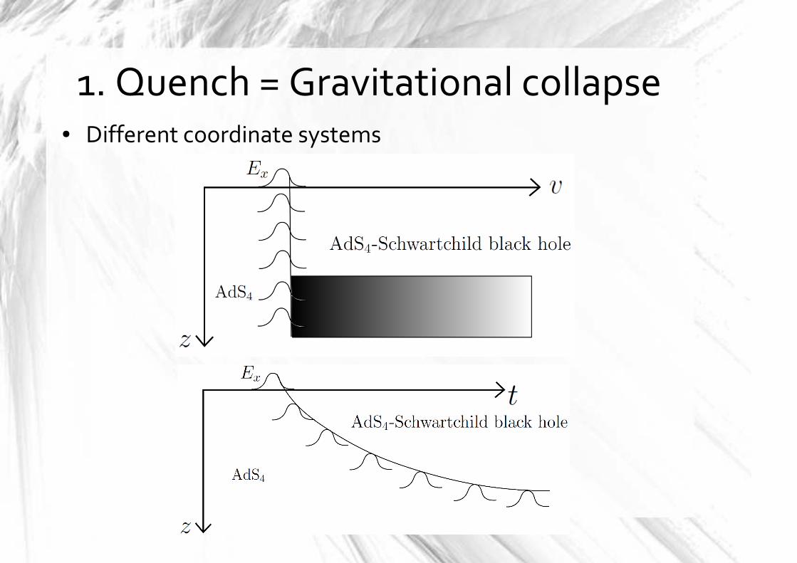
1. Quench = Gravitational collapse● Different coordinate systems

1. Quench = Gravitational collapse● Use the AdS/CFT dictionary to obtain CFT observables
● The current expectation value is given by (Ohm's law)
● The expectation value of energy density satisfies
(Joule heating)
● The expectation values become stationary (and thermal)
immediately when the electric field is turned off

1. Quench = Gravitational collapse● The Vaidya spacetime generalizes to any number of
dimensions
● One has to assume that there is some matter that gives rise to
the appropriate stress energy tensor
● In the following will consider the Vaidya spacetime in 2+1
dimensional bulk as a model for a quench in a 1+1 CFT
● We will consider the case where the mass is a step function
● Want to figure out what happens to correlation functions

2. Review of correlation functions
● Retarded correlators quantify response of a system to
external classical perturbations
● Wightman functions quantify fluctuations in the quantum
state of the system (e.g. occupation numbers of states)
● E.g. harmonic oscillator

2. Review of correlation functions
● In thermal equilibrium the Wightman functions (fluctuations)
and the retarded correlators (response) are related by the
fluctuation dissipation relation
● The density of states

3. Details of the calculation● In the following will consider a scalar field in AdS_3/Vaidya
which is dual to some scalar CFT operator
● Will use the “extrapolate dictionary” to obtain boundary
theory correlators from the bulk correlators
● Most of the time will talk about the bulk correlator, the limit
to boundary does not do anything special

3. Details of the calculation● To obtain the bulk Wightman function, we use the Heisenberg
equation of motion
from which it follows that
● The problem is to solve this 6 dimensional PDE with the initial
data that the correlator at early times agrees with the known
AdS vacuum correlator

3. Details of the calculation● Some technical points:
1) Since we have spatial translational symmetry, we can
→perform a spatial Fourier transform 2x2 dimensional PDE's
→2) The initial data has singularities at short distances Makes
the numerical calculation a bit challenging
3) We solved this problem by using the method of Green's
functions and reduced it to performing integrals over known
→functions Integrate numerically and be careful with the
short distance singularities

4. Results and explanation
● Results:
● The Wightman function seems to approach the thermal one
with a rate given by the lowest quasinormal mode

4. Results an explanation● Quasinormal modes: Poles of the boundary retarded two
point function
● They are actually also poles of the bulk retarded two point
function
● Upon Fourier transforming, the poles become exponentials
● At large timelike separation the retarded correlator decays
exponentially with a rate given by the lowest quasinormal
mode

4. Results and explanation● A useful fact about the retarded correlator is that it satisfies
the Klein-Gordon equation with a delta function source
and the initial condition
● Any initial data for the Klein-Gordon equation can be
propagated in time by using the retarded propagator

4. Results and explanation
1) Sufficiently smooth initial data decays at late times with
the lowest quasinormal mode
2) Initial data with sharp features near the horizon takes long
→time to reach the boundary Starts decaying only after
reflecting from the boundary

4. Results and explanation
● Apply the lessons to the Wightman function
● The initial data has singularities
● Thus, the Wightman function doesn't belong to the 1)
→category Good, since it shouldn't decay to zero!

4. Results and explanation
● But consider the difference
This satisfies the Klein-Gordon equation
and furthermore has no singularities at the initial time
● This is because the singularities are
short distance singularities, which do
not depend on the state of the bulk
scalar

4. Results and explanation
● Thus, we can use the K-G equation to first evolve it with
respect to x_1
This provides smooth initial data f(x_2) that we next evolve
with respect to x_2 to get
Taking the points to the boundary, we get the desired result
● Nothing in the previous discussion relied in the fact that we
are considering AdS_3-Vaidya or on the specific value of the
→mass Expect the conclusion to hold for any d and m

5. Occupation numbers
● Recall the fluctuation dissipation relation in thermal
equilibrium
Thus, in thermal equilibrium the occupation number is given
by a ratio of correlation functions
● We would like to define an effective occupation number in the
non-equilibrium system similarly as a ratio of correlators
● How does one define the Fourier transforms in this case?

5. Occupation numbers
● One way to circumvent the problem: Wigner transform
● Define an effective occupation number as
● This is well defined out of equilibrium and reduces to the
Bose-Einstein distribution in equilibrium

5. Occupation numbers
● Results

5. Occupation numbers
● Results

6. Conclusions and future directions
● The calculations of Wightman (or Feynman) correlators in
holography are very rare
● There are no good simple methods for doing this
● We used a particular method based on the method of Green's
functions. This works for Vaidya spacetime with a sharp theta
function mass, but it does not generalize to any other non-
equilibrium spacetimes
● Thus, new calculational methods are certainly welcome

6. Conclusions and future directions
● We obtained the formula
and I tried arguing this might be true more generally in AdS-
Vaidya than the case we did the numerical calculation for
● Another example where one can easily (analytically) show
that the above is true is in the dual of a “Cardy-Calabrese
state” with a specific boundary state dual to an RP^2 geon
.

6. Conclusions and future directions
● Let's assume that it is generally true in collapsing spacetimes
and see what it would imply
1) Thermalization time scale becomes easy to calculate: just
calculate the quasinormal modes of the final static black hole
2) The “top-down” pattern of holographic thermalization that
has been around in the literature is incorrect for low scaling
→dimension operators It is “bottom-up”
3) CFT correlation functions in far from equilibrium states
thermalize with the same rate as (infinitesimally) small
perturbations around thermal equilibrium

Thanks for listening!

Possible new methods
● One possibility: “mode function approach”
Start from some state where the mode functions and the
expectation values of the creation operators are known (e.g.
vacuum or thermal equilibrium)
● The function f is a solution to the Klein-Gordon equation that
is straightforward to solve numerically in any background
spacetime
● The initial mode function is some known smooth function
(e.g. a Bessel in the case of AdS vacuum)

Possible new methods
● Everything works fine until one plugs the expressions into a
correlation function. One gets expressions of the form
Now the problem is that these integrals do not converge very
fast at large values of the momenta, while numerics usually
breaks down at large momenta
● I don't know how to proceed
● Perhaps one could do something analytically at large
momenta and then patch that to the numerical solution...


![Abstract2 Introduction to the AdS/CFT correspondence The AdS/CFT correspondence, rst suggested by Maldacena [1], is a duality between gravity theory in anti de …](https://static.fdocuments.us/doc/165x107/5e948e6acba06f3abf38eae1/abstract-2-introduction-to-the-adscft-correspondence-the-adscft-correspondence.jpg)


![Gauge/gravity duality ・ Strongly coupled gauge theory ( in large N limit ) ・ String theory gravity in a curved space AdS/CFT [1997, Maldacena] D-brane.](https://static.fdocuments.us/doc/165x107/56649c895503460f94941f4d/gaugegravity-duality-strongly-coupled-gauge-theory-in-large-n-limit.jpg)