Thermal Radiation: The Stefan-Boltzmann Law

Andy Chmilenko, 20310799

Instructor: Tan Dinh

Section 1(Dated: 2:30 pm Wednesday June 26, 2013)

I. PURPOSE

The purpose of this experiment is to verify the Stefan-Boltzmann Law, investigate aspects of blackbody radia-tion such as radiation rates from different surfaces andmeasure their emissivity (ε), investigating the absorptionand transmission of thermal radiation, as well as verifythe inverse square law with respect to the radiative powerof our Stefan-Boltzmann lamp.

II. ANALYSIS

A. Radiation rates from different Surfaces

Cube Thermistor Temperature Sensor reading (mV)

No. Resistance (Ω) T (K) Black White Dull Al Polished Al

9 4,692 378.6 17.4 16.0 2.6 0.9

8 5,500 373.2 16.5 16.2 2.9 1.1

6 13,910 345.6 8.9 9.0 2.6 0.9

5 21,430 334.5 6.4 6.3 1.4 0.6

TABLE I: Thermistor measurements along with the calcu-lated Temperatures for several Leslie cubes, as well as thesensor measurements from the Thermopile for all 4 sides ofthe cubes.

Sample calculations for T using row 1 of Table I

Using values from Table X in the Appendix, for a Ther-mistor Resistance of 4692 Ω, assuming a linear relation-ship between two adjacent resistances corresponding toa difference in 1 degree, using 4760.3 Ω → 105 C and4615.1 Ω → 106 C we can correlate the difference inresistance with the difference in 1 degree.

T = 105C + %Difference · 1C + 273.15CT = 105C + 4760.3−4692

4760.3−4615.1 · 1C + 273.15C

T = 378.6

The distribution function as seen in Eq.1 for the wave-length dependence of emission of thermal radiation bya blackbody at temperature T using Planck’s theory ofquantization.

I(λ, T ) =2πhc2

λ5 · e hcλkT

(1)

and integrating this over all wavelengths the totalpower is simply defined as Eq.2 and including a term ε,

the emissivity, where an emissivity of 1 is a perfect black-body, and 0 < ε < 1 is an imperfect or non-blackbody.

P = εσT 4 (2)

Using the thermopile, several surfaces of different tem-peratures were measured, and the data was compiled intoTable I. Using this data we can calculate the relativeemissivity of each face for all the Leslie cubes assumingthat the black face of the cube has ε = 1, these valuesare compiled in Table II.

Cube Emissivity ε

No. Black White Dull Al Polished Al

9 1 0.92 0.15 0.05

8 1 0.98 0.18 0.07

6 1 1.01 0.29 0.10

5 1 0.98 0.22 0.09

TABLE II: Relative emissivity for all faces of Leslie cubes,assuming the black face has an emissivity of 1

Sample calculations for White emissivity using row1 of Table I, and assuming black emissivity is 1

εwhite = WhiteemissionBlackemission

εwhite = 16.017.4

εwhite = 0.92

Emissivity in this case is independent of temperature,as the temperature decreases the emissivity stays more orless the same as seen in table II with standard deviationvalues in Table III. The dull and polished aluminiumhave some slightly varying emissivity values as the per-cent deviation values are around 28%, but this isn’t toosignificant relative to radiative output compared to theblack surface. The data show that better absorbers arebetter emitters, and poorer absorbers (better reflectors)are poorer emitters like in the case of the aluminium andeven more extreme the polished aluminium compared tothe black or white surfaces.

2

Surface Mean Emissivity Percent

ε Deviation

Black 1 0

White 0.97 4%

Dull Al 0.21 29%

Polish Al 0.08 28%

TABLE III: Mean emissivity and relative percent deviationsfrom the mean for all the surfaces measured in Table II

Sample Calculations Averaging White Emissivity εin Table II using column 3

ε =∑ni εin

ε = 0.92+0.98+1.01+0.984

ε = 0.97

Sample Calculations for White standard deviation σε

in Table II using column 3 and a mean of 0.97

σε =√

1n−1

∑ni (εi − ε)2

σε =

√√√√√ 1

4− 1[(0.92− 0.97)2 + (0.98− 0.97)2+

(1.01− 0.97)2 + (0.98− 0.97)2]

σε =√

130.0043

σε = 3.8× 10−2

Sample Calculations for White percent deviationusing a σε of 3.8 × 10−2 and mean emissivity ε of

0.97 from Table III

%deviation = σεε × 100

%deviation = 3.8×10−20.97 × 100

%deviation = 4%

B. Absorption and transmission of thermalradiation

Cube I0 Iglass Iglass

No. (mV) (mV) I0

9 16.3 0.0 0

9 13.8 0.0 0

TABLE IV: Intensity of thermal radiation of the black surfacemeasured through air and through a pane of glass

Sample Calculations forIglass

I0using Table IV row 1

IglassI0

= 0.016.3 = 0

In this case we didn’t have a strong enough signal tohave any transmission through the glass, but we con-cluded that glass blocks most of the infrared radiationincident on it, as seen in Table IV. In this case, it doesn’tseem like Iglass is dependent on I0.

C. The Stefan Boltzmann law at low temperatures

The thermopile sensor can also be thought of as sourceof thermal radiation since it operates at room tempera-ture. So the net power read by the sensor is the differencefrom the source of radiation it is measuring and the radi-ation from the detector itself since it radiates away someof the energy it is trying to measure. This is given byEq.3

Pnet = Prad − Pdet = εσT 4 − εdetσT 4det (3)

We can try assuming that the Pdet can be neglectedin this experiment because it is low and doesn’t accountfor much difference. Assuming ε = εdet we can rearrangeEq.3 as follows.

Prad = εσT 4 − εdetσT 4det

Prad = εσ(T 4 − T 4det) = εσ(T 4

k − T 4rm)

Prad(T 4k − T 4

rm)= εσ = Const (4)

Since our sensor measurement is directly proportionalto the power of the radiation, we can graph Prad versus(T4

K - Trm4) to confirm weather the Stefan- Boltzmann

equation is correct.

Cube Thermistor Temperature Sensor reading

No. Resistance (Ω) T (K) for Black (mV)

9 4,692 378.6 17.4

8 5,500 373.2 16.5

7 8,160 361.4 10.3

6 13,910 345.6 8.9

5 21,430 334.5 6.4

4 24,120 331.5 5.8

3 54,820 311.5 2.0

2 109,730 296.2 0.3

1 110,320 296.1 0.3

CubeRT 112,220 295.7 0.3

TABLE V: Thermistor measurements along with the calcu-lated Temperatures for several Leslie cubes, as well as thesensor measurements from the Thermopile for the black sideof the cube.

3

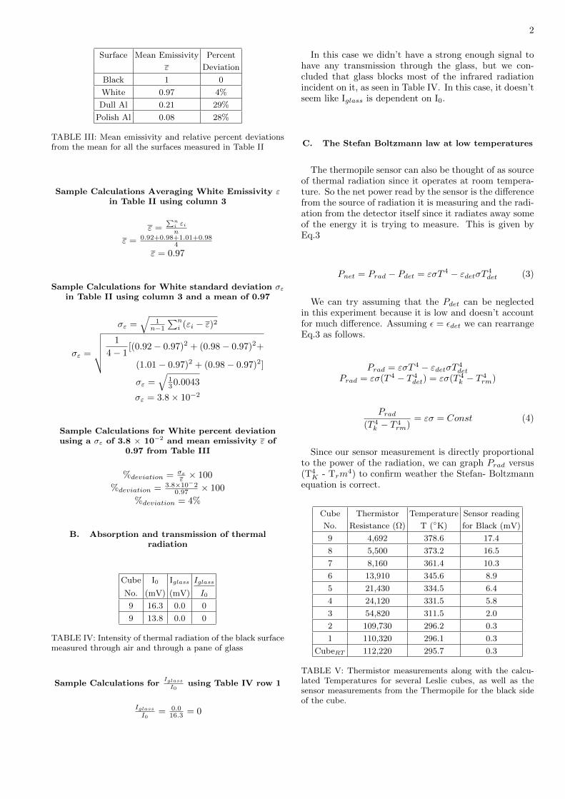
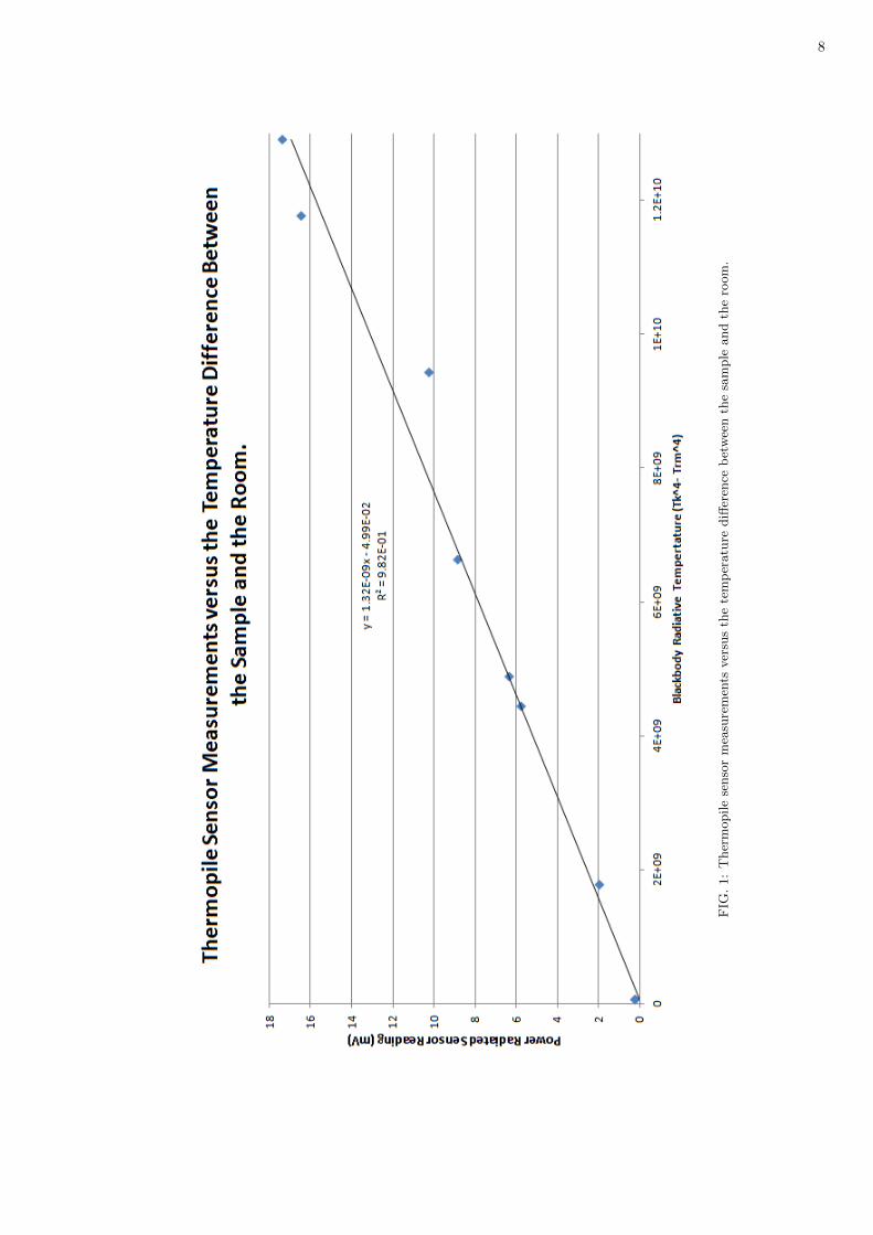
FIG. 1: Thermopile sensor measurements versus the temper-ature difference between the sample and the room.

As seen in Fig.1, we can see that this line fits the datavery well, with one outlier data point with row 3 of TableV, but that withstanding, this proves the relationship ofpower and temperature in the Stefan-Boltzmann equa-tion even at low temperatures.

D. Inverse Square Law

Distance Sensor

(m) Reading (mV)

2.2 0

10 0

20 0

30 0

40 0

50 0

60 0

70 0

80 0

90 0

100 0

TABLE VI: Thermistor measurements of the Stefan-Boltzmann lamp while it was off, for the average ambientmeasurements of the lab.

The average measurements of the lamp from column2 of Table VI was calculated to be 0 mV, there was notenough infrared radiation in the lab to produce any sig-nificant measurements to the sensor.

Distance Sensor

(m) Reading (mV)

2.5 126.1

5 42.4

10 12.7

15 6.1

17 4.8

20 3.5

25 2.3

30 1.6

40 0.8

50 0.5

60 0.3

70 0.2

80 0.0

100 0.0

TABLE VII: Thermistor measurements of the Stefan-Boltzmann lamp running at a voltage of 9.99 V, at variousdistances.

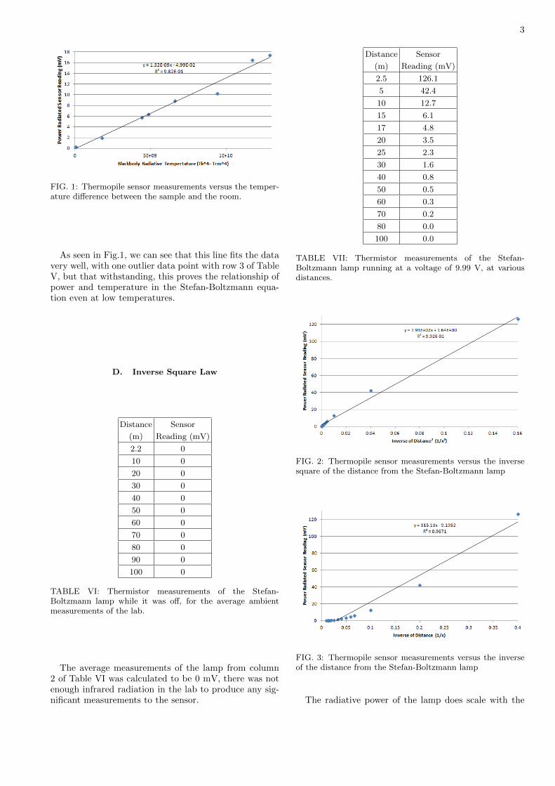
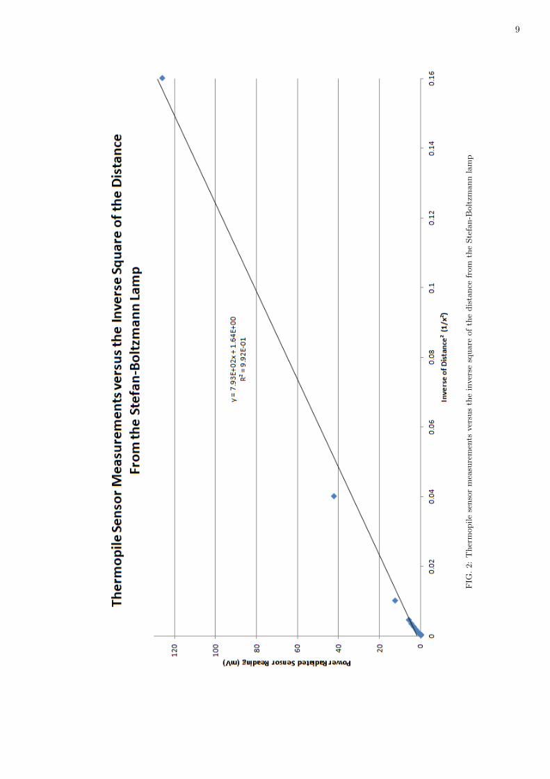
FIG. 2: Thermopile sensor measurements versus the inversesquare of the distance from the Stefan-Boltzmann lamp

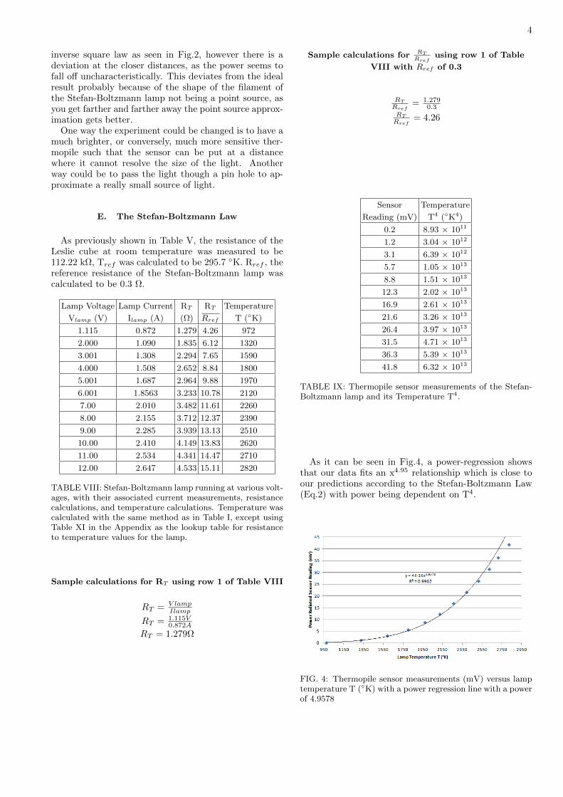
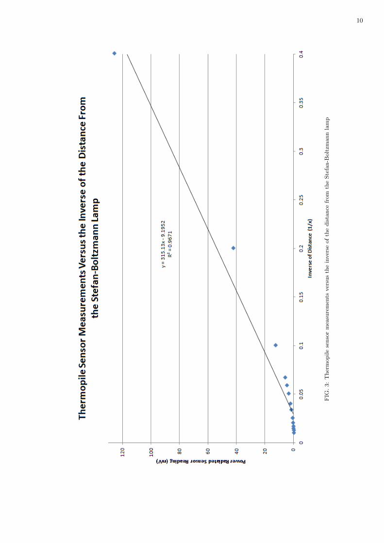
FIG. 3: Thermopile sensor measurements versus the inverseof the distance from the Stefan-Boltzmann lamp

The radiative power of the lamp does scale with the

4

inverse square law as seen in Fig.2, however there is adeviation at the closer distances, as the power seems tofall off uncharacteristically. This deviates from the idealresult probably because of the shape of the filament ofthe Stefan-Boltzmann lamp not being a point source, asyou get farther and farther away the point source approx-imation gets better.

One way the experiment could be changed is to have amuch brighter, or conversely, much more sensitive ther-mopile such that the sensor can be put at a distancewhere it cannot resolve the size of the light. Anotherway could be to pass the light though a pin hole to ap-proximate a really small source of light.

E. The Stefan-Boltzmann Law

As previously shown in Table V, the resistance of theLeslie cube at room temperature was measured to be112.22 kΩ, Tref was calculated to be 295.7 K. Rref , thereference resistance of the Stefan-Boltzmann lamp wascalculated to be 0.3 Ω.

Lamp Voltage Lamp Current RT RT Temperature

Vlamp (V) Ilamp (A) (Ω) Rref T (K)

1.115 0.872 1.279 4.26 972

2.000 1.090 1.835 6.12 1320

3.001 1.308 2.294 7.65 1590

4.000 1.508 2.652 8.84 1800

5.001 1.687 2.964 9.88 1970

6.001 1.8563 3.233 10.78 2120

7.00 2.010 3.482 11.61 2260

8.00 2.155 3.712 12.37 2390

9.00 2.285 3.939 13.13 2510

10.00 2.410 4.149 13.83 2620

11.00 2.534 4.341 14.47 2710

12.00 2.647 4.533 15.11 2820

TABLE VIII: Stefan-Boltzmann lamp running at various volt-ages, with their associated current measurements, resistancecalculations, and temperature calculations. Temperature wascalculated with the same method as in Table I, except usingTable XI in the Appendix as the lookup table for resistanceto temperature values for the lamp.

Sample calculations for RT using row 1 of Table VIII

RT = V lampIlamp

RT = 1.115V0.872A

RT = 1.279Ω

Sample calculations for RTRref

using row 1 of Table

VIII with Rref of 0.3

RTRref

= 1.2790.3

RTRref

= 4.26

Sensor Temperature

Reading (mV) T4 (K4)

0.2 8.93 × 1011

1.2 3.04 × 1012

3.1 6.39 × 1012

5.7 1.05 × 1013

8.8 1.51 × 1013

12.3 2.02 × 1013

16.9 2.61 × 1013

21.6 3.26 × 1013

26.4 3.97 × 1013

31.5 4.71 × 1013

36.3 5.39 × 1013

41.8 6.32 × 1013

TABLE IX: Thermopile sensor measurements of the Stefan-Boltzmann lamp and its Temperature T4.

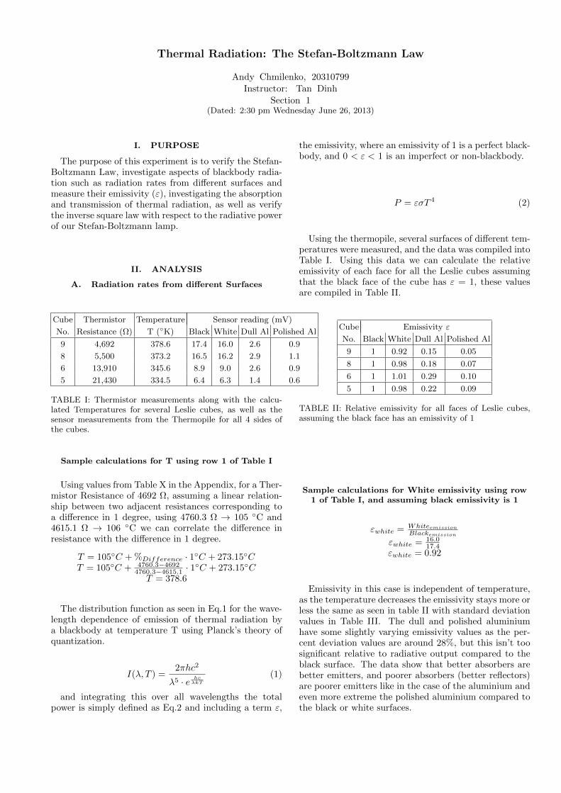
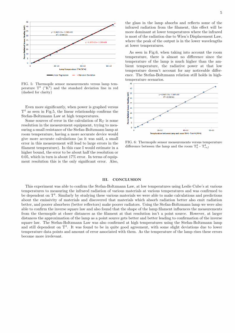
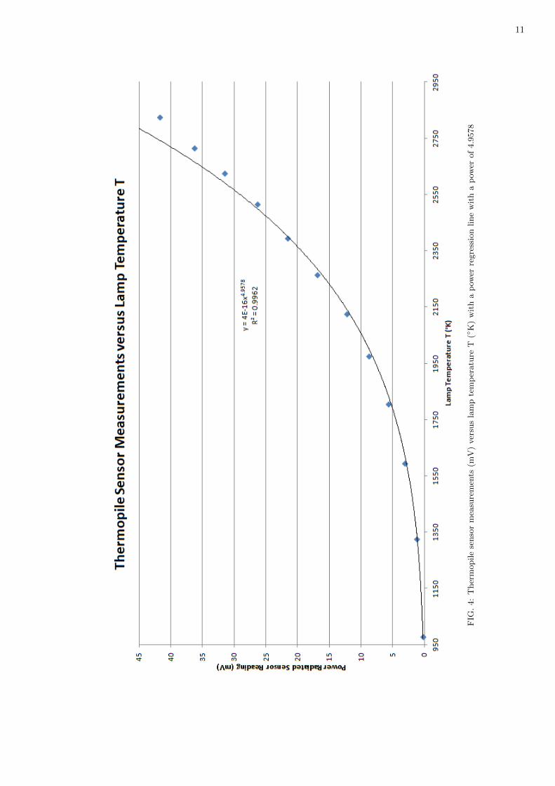
As it can be seen in Fig.4, a power-regression showsthat our data fits an x4.95 relationship which is close toour predictions according to the Stefan-Boltzmann Law(Eq.2) with power being dependent on T4.

FIG. 4: Thermopile sensor measurements (mV) versus lamptemperature T (K) with a power regression line with a powerof 4.9578

5

FIG. 5: Thermopile sensor measurements versus lamp tem-perature T4 (K4) and the standard deviation line in red(dashed for clarity)

Even more significantly, when power is graphed versusT4 as seen in Fig.5, the linear relationship confirms theStefan-Boltzmann Law at high temperatures.

Some sources of error in the calculation of RT is someresolution in the measurement equipment, trying to mea-suring a small resistance of the Stefan-Boltzmann lamp atroom temperature, having a more accurate device wouldgive more accurate calculations (as it was said, a smallerror in this measurement will lead to large errors in thefilament temperature). In this case I would estimate in ahigher bound, the error to be about half the resolution or0.05, which in turn is about 17% error. In terms of equip-ment resolution this is the only significant error. Also,

the glass in the lamp absorbs and reflects some of theinfrared radiation from the filament, this effect will bemore dominant at lower temperatures where the infraredis most of the radiation due to Wien’s Displacement Law,where the peak of the output is in the lower wavelengthsat lower temperatures.

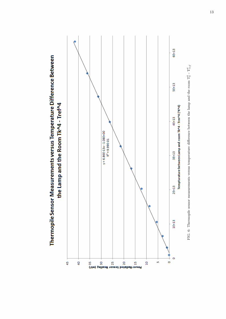
As seen in Fig.6, when taking into account the roomtemperature, there is almost no difference since thetemperature of the lamp is much higher than the am-bient temperature, the radiative power at that lowtemperature doesn’t account for any noticeable differ-ence. The Stefan-Boltzmann relation still holds in high-temperature scenarios.

FIG. 6: Thermopile sensor measurements versus temperaturedifference between the lamp and the room T4

k - T4ref

III. CONCLUSION

This experiment was able to confirm the Stefan-Boltzmann Law, at low temperatures using Leslie Cube’s at varioustemperatures to measuring the infrared radiation of various materials at various temperatures and was confirmed tobe dependent on T4. Similarly by studying these various materials we were able to make calculations and predictionsabout the emissivity of materials and discovered that materials which absorb radiation better also emit radiationbetter, and poorer absorbers (better reflectors) make poorer radiators. Using the Stefan-Boltzmann lamp we were alsoable to confirm the inverse square law and also found that the shape of the lamp filament influences the measurementsfrom the thermopile at closer distances as the filament at that resolution isn’t a point source. However, at largerdistances the approximation of the lamp as a point source gets better and better leading to confirmation of the inversesquare law. The Stefan-Boltzmann Law was also confirmed at high temperatures using the Stefan-Boltzmann lampand still dependent on T4. It was found to be in quite good agreement, with some slight deviations due to lowertemperature data points and amount of error associated with them. As the temperature of the lamp rises these errorsbecome more irrelevant.

6

Appendices

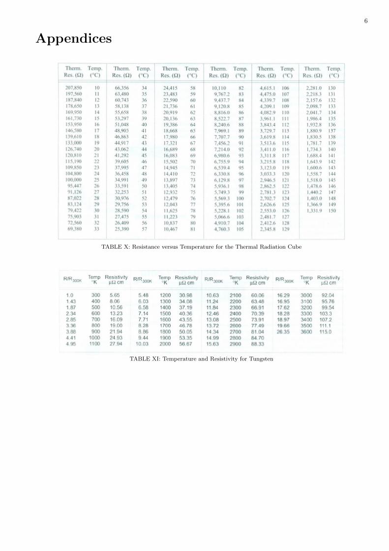
TABLE X: Resistance versus Temperature for the Thermal Radiation Cube

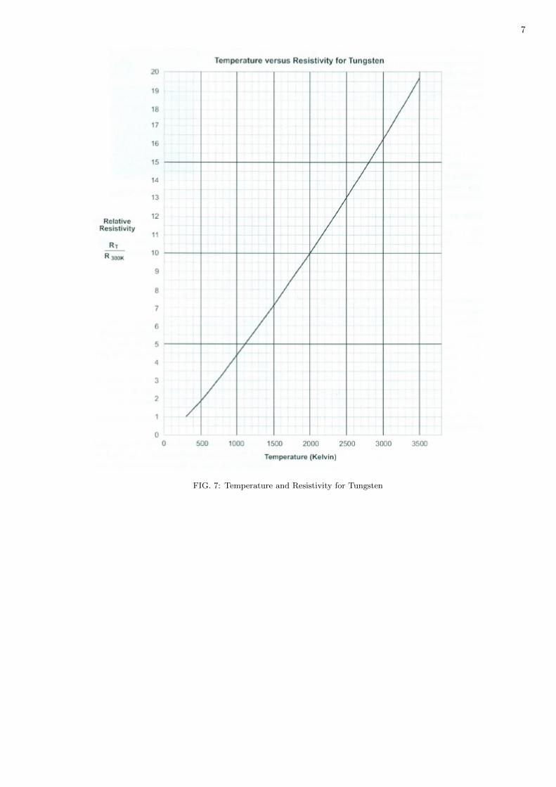
TABLE XI: Temperature and Resistivity for Tungsten

7

FIG. 7: Temperature and Resistivity for Tungsten

8

FIG

.1:

Ther

mopile

senso

rm

easu

rem

ents

ver

sus

the

tem

per

atu

rediff

eren

ceb

etw

een

the

sam

ple

and

the

room

.

9

FIG

.2:

Ther

mopile

senso

rm

easu

rem

ents

ver

sus

the

inver

sesq

uare

of

the

dis

tance

from

the

Ste

fan-B

olt

zmann

lam

p

10

FIG

.3:

Ther

mopile

senso

rm

easu

rem

ents

ver

sus

the

inver

seof

the

dis

tance

from

the

Ste

fan-B

olt

zmann

lam

p

11

FIG

.4:

Ther

mopile

senso

rm

easu

rem

ents

(mV

)ver

sus

lam

pte

mp

eratu

reT

(K

)w

ith

ap

ower

regre

ssio

nline

wit

ha

pow

erof

4.9

578

12

FIG

.5:

Ther

mopile

senso

rm

easu

rem

ents

ver

sus

lam

pte

mp

eratu

reT

4(

K4)

and

the

standard

dev

iati

on

line

inre

d(d

ash

edfo

rcl

ari

ty)

13

FIG

.6:

Ther

mopile

senso

rm

easu

rem

ents

ver

sus

tem

per

atu

rediff

eren

ceb

etw

een

the

lam

pand

the

room

T4 k

-T

4 ref