Thermal energy storage in metallic phase change · PDF fileThermal energy storage in PCMs...

Thermal energy storage in metallic phase change

materials

by

Johannes Paulus Kotzé

Dissertation presented for the degree of Doctor of Philosophy in the Faculty of Engineering at

Stellenbosch University

Promoter: Prof. Theodor Willem Von Backström

Co-Promoter: Dr. Paul Johan Erens

December 2014

The financial assistance of the National Research Foundation (NRF) towards this

research is hereby acknowledged. Opinions expressed and conclusions arrived at

are those of the author and are not necessarily to be attributed to the NRF.

i

Declaration

By submitting this dissertation electronically, I declare that the entirety of the

work contained therein is my own, original work, that I am the sole author thereof

(save to the extent explicitly otherwise stated), that reproduction and publication

thereof by Stellenbosch University will not infringe any third party rights and that

I have not previously in its entirety or in part submitted it for obtaining any

qualification.

This dissertation includes one original paper published in a peer-reviewed journal,

two peer reviewed conference papers, three conference papers and one

unpublished publication. The development and writing of these papers (published

and unpublished) were the principal responsibility of myself and, for each of the

cases where this is not the case, a declaration is included in the dissertation

indicating the nature and extent of the contributions of co-authors.

Date: _________________

Copyright © 2014 Stellenbosch University

All rights reserved

Stellenbosch University http://scholar.sun.ac.za

ii

Abstract

Currently the reduction of the levelised cost of electricity (LCOE) is the main goal

of concentrating solar power (CSP) research. Central to a cost reduction strategy

proposed by the American Department of Energy is the use of advanced power

cycles like supercritical steam Rankine cycles to increase the efficiency of the

CSP plant. A supercritical steam cycle requires source temperatures in excess of

620°C, which is above the maximum storage temperature of the current two-tank

molten nitrate salt storage, which stores thermal energy at 565°C. Metallic phase

change materials (PCM) can store thermal energy at higher temperatures, and do

not have the drawbacks of salt based PCMs. A thermal energy storage (TES)

concept is developed that uses both metallic PCMs and liquid metal heat transfer

fluids (HTF). The concept was proposed in two iterations, one where steam is

generated directly from the PCM – direct steam generation (DSG), and another

where a separate liquid metal/water heat exchanger is used – indirect steam

generation, (ISG). Eutectic aluminium-silicon alloy (AlSi12) was selected as the

ideal metallic PCM for research, and eutectic sodium-potassium alloy (NaK) as

the most suitable heat transfer fluid.

Thermal energy storage in PCMs results in moving boundary heat transfer

problems, which has design implications. The heat transfer analysis of the heat

transfer surfaces is significantly simplified if quasi-steady state heat transfer

analysis can be assumed, and this is true if the Stefan condition is met. To validate

the simplifying assumptions and to prove the concept, a prototype heat storage

unit was built. During testing, it was shown that the simplifying assumptions are

valid, and that the prototype worked, validating the concept. Unfortunately

unexpected corrosion issues limited the experimental work, but highlighted an

important aspect of metallic PCM TES. Liquid aluminium based alloys are highly

corrosive to most materials and this is a topic for future investigation.

To demonstrate the practicality of the concept and to come to terms with the

control strategy of both proposed concepts, a storage unit was designed for a

100 MW power plant with 15 hours of thermal storage. Only AlSi12 was used in

the design, limiting the power cycle to a subcritical power block. This

demonstrated some practicalities about the concept and shed some light on control

issues regarding the DSG concept.

A techno-economic evaluation of metallic PCM storage concluded that metallic

PCMs can be used in conjunction with liquid metal heat transfer fluids to achieve

high temperature storage and it should be economically viable if the corrosion

issues of aluminium alloys can be resolved. The use of advanced power cycles,

metallic PCM storage and liquid metal heat transfer is only merited if significant

reduction in LCOE in the whole plant is achieved and only forms part of the

solution. Cascading of multiple PCMs across a range of temperatures is required

to minimize entropy generation. Two-tank molten salt storage can also be used in

conjunction with cascaded metallic PCM storage to minimize cost, but this also

needs further investigation.


iii

Opsomming

Tans is die minimering van die gemiddelde leeftydkoste van elektrisiteit (GLVE)

die hoofdoel van gekonsentreerde son-energie navorsing. In die

kosteverminderingsplan wat voorgestel is deur die Amerikaanse Departement van

Energie, word die gebruik van gevorderde kragsiklusse aanbeveel. 'n Superkritiese

stoom-siklus vereis bron temperature hoër as 620 °C, wat bo die 565 °C

maksimum stoor temperatuur van die huidige twee-tenk gesmelte nitraatsout

termiese energiestoor (TES) is. Metaal fase veranderingsmateriale (FVMe) kan

termiese energie stoor by hoër temperature, en het nie die nadele van

soutgebaseerde FVMe nie. ŉ TES konsep word ontwikkel wat gebruik maak van

metaal FVM en vloeibare metaal warmteoordrag vloeistof. Die konsep is

voorgestel in twee iterasies; een waar stoom direk gegenereer word uit die FVM

(direkte stoomopwekking (DSO)), en 'n ander waar 'n afsonderlike vloeibare

metaal/water warmteruiler gebruik word (indirekte stoomopwekking (ISO)).

Eutektiese aluminium-silikon allooi (AlSi12) is gekies as die mees geskikte

metaal FVM vir navorsingsdoeleindes, en eutektiese natrium – kalium allooi

(NaK) as die mees geskikte warmteoordrag vloeistof.

Termiese energie stoor in FVMe lei tot bewegende grens warmteoordrag

berekeninge, wat ontwerps-implikasies het. Die warmteoordrag ontleding van die

warmteruilers word aansienlik vereenvoudig indien kwasi-bestendige toestand

warmteoordrag ontledings gebruik kan word en dit is geldig indien daar aan die

Stefan toestand voldoen word. Om vereenvoudigende aannames te bevestig en om

die konsep te bewys is 'n prototipe warmte stoor eenheid gebou. Gedurende toetse

is daar bewys dat die vereenvoudigende aannames geldig is, dat die prototipe

werk en dien as ŉ bevestiging van die konsep. Ongelukkig het onverwagte

korrosie die eksperimentele werk kortgeknip, maar dit het klem op 'n belangrike

aspek van metaal FVM TES geplaas. Vloeibare aluminium allooie is hoogs

korrosief en dit is 'n onderwerp vir toekomstige navorsing.

Om die praktiese uitvoerbaarheid van die konsep te demonstreer en om die

beheerstrategie van beide voorgestelde konsepte te bevestig is 'n stoor-eenheid

ontwerp vir 'n 100 MW kragstasie met 15 uur van 'n TES. Slegs AlSi12 is gebruik

in die ontwerp, wat die kragsiklus beperk het tot 'n subkritiese stoomsiklus. Dit

het praktiese aspekte van die konsep onderteken, en beheerkwessies rakende die

DSO konsep in die kollig geplaas.

In 'n tegno-ekonomiese analise van metaal FVM TES word die gevolgtrekking

gemaak dat metaal FVMe gebruik kan word in samewerking met 'n vloeibare

metaal warmteoordrag vloeistof om hoë temperatuur stoor moontlik te maak en

dat dit ekonomies lewensvatbaar is indien die korrosie kwessies van aluminium

allooi opgelos kan word. Die gebruik van gevorderde kragsiklusse, metaal FVM

stoor en vloeibare metaal warmteoordrag word net geregverdig indien beduidende

vermindering in GLVE van die hele kragsentrale bereik is, en dit vorm slegs 'n

deel van die oplossing. ŉ Kaskade van verskeie FVMe oor 'n reeks van

temperature word vereis om entropie generasie te minimeer. Twee-tenk gesmelte

soutstoor kan ook gebruik word in samewerking met kaskade metaal FVM stoor

om koste te verminder, maar dit moet ook verder ondersoek word.


iv

Acknowledgements

I would like to acknowledge the following people:

My promoters: Prof. T.W von Backström and Dr. P.J. Erens, for your time and for

supervising me throughout this project.

My siblings, Ilze, Pieter, Hannetjie, Koot and Alwyn who always supported me

with love and incredible friendship, you are my best friends.

My parents Koot and Marianne, whose unconditional love and support are never-

ending, which really is a base of stability in my life. Dad, you are truly my mentor

and the greatest engineer I know. Mom, you are like a cool breeze on a hot

summer’s day.

Alexandra, your friendship, love and endless prayers carried me more than you

know.

The staff of the Mechanical and Mechatronic Department.

All the members of STERG.

The NRF/DST, CRSES and STERG for funding.

ESTEQ for making FLOWNEX available free of charge.

Mrs. Banks, you gave me a second chance, and without your experience and

knowledge, none of this would be possible.

The late Prof. Detlev Kröger, you were an inspiration to all of us.


v

“My grace is sufficient for thee: for my strength is made perfect in weakness.”

2 Cor 12:9


vi

Table of contents

Page

List of figures .......................................................................................................... ix

List of tables .......................................................................................................... xiv

Nomenclature ........................................................................................................ xvi

Important dimensionless numbers ......................................................................... xx

1 Introduction .................................................................................................... 1

2 Literature review and project goals ................................................................ 3

2.1 Cost breakdown of CSP and strategies for cost reduction.................. 4

2.2 Factors determining thermal efficiency .............................................. 5

2.3 Power cycles ....................................................................................... 9

2.4 Overview of thermal energy storage and current technical limitations10

2.4.1 Current state of the art ...................................................... 11

2.4.2 High temperature storage concepts .................................. 14

2.5 Thermal energy storage in phase change materials .......................... 17

2.5.1 Eutectic materials ............................................................. 18

2.5.2 Comparison of some PCMs ............................................. 19

2.6 AlSi12 as a PCM in literature ........................................................... 21

2.7 Heat transfer fluids and current technical limitations ....................... 27

2.7.1 Thermal oil ....................................................................... 28

2.7.2 Molten salt........................................................................ 29

2.7.3 Direct steam ..................................................................... 30

2.7.4 Air or gas .......................................................................... 30

2.7.5 Sodium ............................................................................. 30

2.7.6 NaK .................................................................................. 31

2.7.7 Conclusion ....................................................................... 32

2.8 Conclusion and project scope ........................................................... 33

3 Thermal energy storage concept ................................................................... 35

3.1 Direct steam generator ...................................................................... 35

3.2 Indirect steam generator ................................................................... 37

4 Material properties ....................................................................................... 39

4.1 The properties and characteristics of AlSi12 .................................... 39


vii

4.1.1 Thermal and physical properties of eutectic Aluminium

silicon alloy ...................................................................... 40

4.2 The properties and characteristics of NaK ....................................... 42

4.2.1 Physical properties ........................................................... 43

4.2.2 Safety ............................................................................... 46

4.2.3 Steam generator design .................................................... 47

4.3 Other materials ................................................................................. 48

5 Flownex ........................................................................................................ 49

6 Heat transfer mechanisms ............................................................................ 51

6.1 Liquid metal heat transfer ................................................................. 51

6.2 Convective boiling heat transfer inside plain tubes .......................... 52

7 Moving boundary heat trasnfer around vertical heat transfer tubes ............. 53

7.1 Analysis of the moving boundary system and transient analysis ..... 54

7.2 Instantaneous heat transfer ............................................................... 58

7.3 Numerical solution to the moving boundary problem for transient

analysis ............................................................................................. 60

7.4 Prototype and experimental setup..................................................... 66

7.4.1 Heating elements .............................................................. 71

7.4.2 Cooling system ................................................................. 72

7.4.3 Thermal insulation and losses .......................................... 75

7.4.4 Measurements and data acquisition ................................. 76

7.5 Experiment ....................................................................................... 78

7.6 Numerical simulation ....................................................................... 80

7.7 Comparison and conclusions ............................................................ 81

8 Preliminary plant design and simulation ...................................................... 85

8.1 Power generating cycle ..................................................................... 85

8.2 Primary heat transfer loop ................................................................ 89

8.2.1 Primary loop heat transfer requirements .......................... 90

8.2.2 Receiver sizing ................................................................. 95

8.3 Storage sizing ................................................................................... 99

8.4 Heat exchanger sizing and modelling ............................................. 101

8.4.1 Steam/water Heat exchangers for the DSG concept ...... 104

8.4.2 NaK heat exchangers for the DSG concept ................... 107


viii

8.4.3 Heat exchangers for the ISG concept ............................. 108

8.5 Overall model ................................................................................. 111

8.6 Conclusion and practical considerations ........................................ 114

8.6.1 Feasibility of the DSG concept ...................................... 114

8.6.2 Thermodynamic considerations and cascaded thermal

energy storage. ............................................................... 114

9 High temperature corrosion of AlSi12 ....................................................... 118

10 Techno-economic feasibility ...................................................................... 121

11 Future work ................................................................................................ 128

11.1 Axial conduction and CFD models ................................................ 128

11.2 Material testing ............................................................................... 128

11.3 More alloys and investigation into hyper-eutectics ........................ 129

11.4 High temperature corrosion resistance, heat exchangers and

containment .................................................................................... 129

11.5 The use of liquid metals in CSP ..................................................... 129

11.6 Analysis of a combined molten salt storage system with metallic

PCM storage ................................................................................... 130

11.7 Optimisation through entropy minimization .................................. 130

12 Conclusion .................................................................................................. 131

13 References .................................................................................................. 134

Appendix A Candidate phase change materials ................................. 140

Appendix B Properties of NaK........................................................... 144

Appendix C Derivation of the Stefan number .................................... 147

Appendix D Experimental design ....................................................... 150

D.1 Certificates of analysis and calibration ................................................ 150

D.2 Laminar flow meter design detail ........................................................ 153

Appendix E Prediction of thermal losses of the test section .............. 158

Appendix F Heat transfer measurements ........................................... 160

F.1 Measurement of heat transfer from PCM to Oil .................................. 160

F.2 Measurement of heat transfer from Oil to Water ................................. 161

Appendix G Simulation Code ............................................................. 162

Appendix H Thermodynamic analysis of the steam cycle ................. 166

Appendix I Flownex model ............................................................... 171


ix

List of figures

Page

Figure 1 - Efficiency of a receiver at various concentration ratios .......................... 7

Figure 2 – Approximate thermal efficiency of a steam cycle at increasing source

temperatures for a sink temperature of 40°C ........................................................... 7

Figure 3 - Thermal efficiency of a CSP plant at different concentration ratios for a

sink temperature of 40°C ......................................................................................... 8

Figure 4 - Modes of thermal energy storage .......................................................... 10

Figure 5 – Classification of TES concepts ............................................................. 11

Figure 6 - Two tank molten salt TES for central receivers (Direct system) .......... 13

Figure 7 - Two tank molten salt TES system for parabolic trough (Indirect)

(Herrmann, et al., 2006) ......................................................................................... 13

Figure 8 - Graphite heat transfer enhancements for low thermal diffusivity in

PCMs (Tamme, 2007) ............................................................................................ 16

Figure 9 - Concrete storage with heat exchanger pipes visible at the end (Tamme,

2007) ...................................................................................................................... 16

Figure 10 - Generic phase diagram for a binary eutectic system ........................... 19

Figure 11 - Comparison of high temperature PCMs found in literature (Latent heat

of fusion against temperature) ............................................................................... 20

Figure 12 - Metallic phase change materials found in literature (Birchenall, et al.,

1979) ...................................................................................................................... 21

Figure 13 - Analytical comparison of the charging rate of a metallic PCM versus a

salt PCM (Hoshi, et al., 2005 ) .............................................................................. 22

Figure 14 - Steam generator as proposed by Adinberg et al. (2010) ..................... 22

Figure 15 - Thermal storage around a catalyst to reduce the light-up time for a

catalytic converter .................................................................................................. 23

Figure 16 - Catalytic converter with PCM TES system ........................................ 23

Figure 17 - Test results from catalytic converter tests ........................................... 24

Figure 18 - Waste heat recovery unit using AlSi12 as PCM ................................. 24

Figure 19 - Temperature readouts for thermocouples in the storage unit through

discharge ................................................................................................................ 25

Figure 20 - Space heater with latent heat storage (Wang, et al., 2004) ................. 25

Figure 21 - Sectioned view of the space heater (Wang, et al., 2004) .................... 26

Figure 22 - Section through the space heater (Wang, et al., 2004) ........................ 26

Figure 23 - Test results for 1540 W heating power (Wang, et al., 2004) .............. 27


x

Figure 24 - Sodium-Potassium eutectic system (Liquid metal engineering center,

1972) ...................................................................................................................... 32

Figure 25 - Comparison of HTF operative temperatures ....................................... 33

Figure 26 - Direct steam generator concept ........................................................... 36

Figure 27 - Power cycle with the direct steam generation concept ....................... 37

Figure 28 - Indirect steam generation concept ....................................................... 38

Figure 29 - Power cycle with the indirect steam generation concept .................... 38

Figure 30 - Aluminium-Silicon eutectic system (Murray, et al., 1984)................. 40

Figure 31 - Thermal diffusivity of eutectic NaK ................................................... 45

Figure 32 - Prandtl number of eutectic NaK .......................................................... 45

Figure 33 – Flownex model of a Rankine cycle .................................................... 49

Figure 34 – Discretization and two dimensional models for charging and

discharging ............................................................................................................. 53

Figure 35 - Hexagonal elements showing solidified PCM cylinders touching ..... 54

Figure 36 - Problem description ............................................................................ 55

Figure 37 - Stefan number as a function of wall temperature ............................... 58

Figure 38 - Resistance heat transfer model for charging and discharging ............. 59

Figure 39 - Discretisation of the heat transfer problem ......................................... 60

Figure 40 - Resistances between elements ............................................................ 61

Figure 41 - T-H diagram for a eutectic or pure metal ............................................ 63

Figure 42 - Enthalpy method algorithm ................................................................. 65

Figure 43 - Cross section of the test section .......................................................... 66

Figure 44 – Test section ......................................................................................... 67

Figure 45 – Empty test section .............................................................................. 69

Figure 46 - Casting of AlSi12 into test section ...................................................... 69

Figure 47 - Test section suspended in frame with heating elements and cladding

(cladding still open) ............................................................................................... 70

Figure 48 - Ceramic band heater ............................................................................ 71

Figure 49 - Wiring of the three band heaters ......................................................... 72

Figure 50 – Band heaters installed around the storage vessel ............................... 72

Figure 51 – Test rig process diagram ..................................................................... 73

Figure 52 - Flownex model used to design the experiment ................................... 74

Figure 53 – The experimental setup ...................................................................... 76


xi

Figure 54 - Heat transfer measurements ................................................................ 79

Figure 55 - Thermocouple readouts throughout discharge of the storage system . 80

Figure 56 - Simulation results of the phase change problem based on the

experimental ........................................................................................................... 81

Figure 57 - Experimental data and simulation data plotted over each other for

comparison ............................................................................................................. 82

Figure 58 - Comparison between the positions of solidification front as predicted

by the simulation and measured in the prototype .................................................. 83

Figure 59 - Quasi steady conduction problem ....................................................... 83

Figure 60 - Temperature distribution through melt as the solidification front

passes thermocouple #5 ......................................................................................... 84

Figure 61 - Overview of the model ........................................................................ 85

Figure 62 - Power generation cycle ....................................................................... 86

Figure 63 - T-s diagram for the power cycle ......................................................... 87

Figure 64 - Flownex model of the Rankine Cycle ................................................. 89

Figure 65 - Heat exchanger configuration for the DSG concept ........................... 90

Figure 66 - Annual DNI for South Africa (Geosun) .............................................. 91

Figure 67 - Clear sky DNI for Upington ................................................................ 91

Figure 68 - Normalized DNI for the summer solstice, winter solstice and the

southward equinox (spring) for Upington ............................................................. 92

Figure 69 - Energy balance to storage ................................................................... 93

Figure 70 - Power to and from storage .................................................................. 94

Figure 71 - External receiver ................................................................................. 95

Figure 72 - Liquid sodium receiver tested at PSA (Schiel, 1988) ......................... 96

Figure 73 - Pressure drop over receiver versus outer diameter for various B36.19

tubes ....................................................................................................................... 98

Figure 74 – Receiver model ................................................................................... 99

Figure 75 – Heat transfer sizing ........................................................................... 102

Figure 76 - Boiler arrangement ............................................................................ 104

Figure 77 – Boiler model ..................................................................................... 105

Figure 78 - Re-heater and super-heater arrangement ........................................... 105

Figure 79 – Re-heater and super-heater model .................................................... 106

Figure 80 – ISG heat transfer and storage ........................................................... 109

Figure 81 - Primary cooling loop for the ISG concept ........................................ 109


xii

Figure 82 – Calculation of charge state and moving boundary position ............. 111

Figure 83 – Screenshot of the overall Flownex model for the DSG concept ...... 112

Figure 84 – Screenshot of the overall Flownex model for the ISG concept ........ 113

Figure 85 - Entropy generation between the primary cooling loop and the PCM

............................................................................................................................. 116

Figure 86 – Single PCM storage in the DSG concept ......................................... 116

Figure 87 – Single PCM storage in the ISG concept ........................................... 117

Figure 88 – Cascaded PCMs for the DSG concept .............................................. 117

Figure 89 - Microstructure of inter-metallic zone (Bouayad, et al., 2003) .......... 118

Figure 90 - Aluminium-iron eutectic system ....................................................... 119

Figure 91 - Electron-micrograph of a surface treated steel sample after corrosion

testing. (Deqing, et al., 2003) ............................................................................... 120

Figure 92 – Material cost of metallic PCMs versus melting temperature. .......... 123

Figure 93 – Single metallic PCM storage to enable supercritical steam ............. 126

Figure 94 – T-s diagram of a supercritical steam cycle for combined storage .... 126

Figure 95 - Density of eutectic NaK .................................................................... 144

Figure 96 - Dynamic viscosity of NaK ................................................................ 144

Figure 97 - Kinematic viscosity of eutectic NaK ................................................ 145

Figure 98 - Thermal conductivity of eutectic NaK .............................................. 145

Figure 99 - Specific heat of eutectic NaK ............................................................ 146

Figure 100 - Temperature profiles during one-dimensional freezing of a liquid

initially at T∞ ........................................................................................................ 147

Figure 101 - Chemical analysis of aluminium alloy cast into the test section ..... 150

Figure 102 - Certification of compliance for K-type thermocouples .................. 152

Figure 103 - Calibration certificate - water flow meter ....................................... 152

Figure 104 - Laminar flow meter drawing ........................................................... 154

Figure 105 - Calibration curve for the Endress+Hauser Deltabar S PMD75

pressure transducer .............................................................................................. 154

Figure 106 - Kinematic viscosity of the ISO 100 heat transfer oil ...................... 155

Figure 107 - Kinematic viscosity of ISO 100 oil as a function of temperature ... 156

Figure 108 - Dynamic viscosity of ISO100 oil as a function of temperature ...... 156

Figure 109 - Calibration curve for the flow meter at 42.5°C ............................... 157

Figure 110 - Heat transfer rates from PCM to oil ................................................ 160


xiii

Figure 111 - Heat transfer from oil to water ........................................................ 161

Figure 112 - Steam Rankine cycle ....................................................................... 166

Figure 113 - T-S diagram for the Rankine steam cycle ....................................... 167

Figure 114 - Flownex model of the steam Rankine cycle ................................... 171

Figure 115 - HP turbine settings .......................................................................... 172

Figure 116 - LP turbine settings .......................................................................... 172

Figure 117 - LP Pump chart ................................................................................. 173

Figure 118 - HP pump chart ................................................................................ 173


xiv

List of tables

Page

Table 1 - Cost breakdown of CSP (Kolb, et al., 2011) ............................................ 4

Table 2 - Notable examples of thermal energy storage (Medrano, et al., 2010) ... 12

Table 3 - Thermal properties of nitrate salts .......................................................... 14

Table 4 - Candidate materials for sensible thermal energy storage (Gil, et al.,

2010) ...................................................................................................................... 15

Table 5 - Properties of heat transfer fluids ............................................................ 28

Table 6 - Composition specifications of LM6 alloy (BS 1490:1988 LM6) .......... 39

Table 7 - General material properties of eutectic AlSi12 alloy (Matbase) ............ 41

Table 8 - Thermal properties used by He et al. (He, et al., 2001) ......................... 41

Table 9 - Thermophysical properties of AlSi12 as used by Wang et al. ............... 41

Table 10 - Properties of AlSi12 ............................................................................. 42

Table 11 – Thermal properties of low carbon steel and stainless steel 304 ........... 48

Table 12 - Test section geometry ........................................................................... 68

Table 13 - Chemical analysis of the cast aluminium alloy .................................... 70

Table 14 - Properties of ISO 100 quenching oil (Kopeliovich, 2013) ................... 73

Table 15 - Cooling loop component details ........................................................... 75

Table 16 - Thermal resistance of insulating layers around the storage unit .......... 75

Table 17 - Measurement errors on the test section thermocouples ........................ 77

Table 18 - Measurement devices and calibration points ........................................ 78

Table 19 - Energy balance during latent heat discharge ........................................ 79

Table 20 - Energy balance of a hypothetical power cycle ..................................... 88

Table 21 - Boundary conditions and heat transfer requirements of the steam

generator ................................................................................................................ 88

Table 22 - Heat transfer requirements for the primary heat transfer loop ............. 94

Table 23 – Typical receiver peak flux design values (Battleson, 1981) ................ 96

Table 24 - Pressure drop for various heat transfer tube diameters for the receiver

............................................................................................................................... 98

Table 25 - Receiver geometry and performance parameters ................................. 99

Table 26 - Mass and volume required for 15h of thermal energy storage ........... 100

Table 27 - Size of the storage tanks ..................................................................... 100


xv

Table 28 - ISG storage sizing .............................................................................. 100

Table 29 – Summary of material property databases used in Flownex ............... 102

Table 30 – Summary of correlations used in the Flownex simulations ............... 103

Table 31 – Steam water heat exchanger geometry .............................................. 106

Table 32 – Steam/water heat exchanger control strategy .................................... 107

Table 33 – NaK flow distribution ........................................................................ 107

Table 34 – NaK heat exchanger geometry for the DSG concept ......................... 108

Table 35 – NaK heat exchanger geometry, storage tank dimensions and

operational parameters ......................................................................................... 110

Table 36 – Material cost of eutectic nitrate salt ................................................... 121

Table 37 – Constituent metal prices .................................................................... 122

Table 38 – Material cost of a select number of metallic PCMs ........................... 122

Table 39 – Overall cost estimates of metallic PCMs ........................................... 123

Table 40 – Predicted reduction in LCOE ............................................................. 125

Table 41 – Enthalpy of steam in a supercritical steam generator ........................ 127

Table 42 – Carbonates (Kenisarin, 2009) ............................................................ 140

Table 43 – Hydroxides (Kenisarin, 2009) ........................................................... 140

Table 44 – Chlorides (Kenisarin, 2009) ............................................................... 141

Table 45 – Fluorides (Kenisarin, 2009) ............................................................... 142

Table 46 – Metals (Kenisarin, 2009) ................................................................... 143

Table 47 – Nitrates (Kenisarin, 2009) ................................................................. 143

Table 48 - Design parameters of the laminar flow meter .................................... 153

Table 49 - Laminar flow meter critical geometry ................................................ 153

Table 50 – Geometry, properties and conditions for heat loss estimation ........... 158

Table 51 – Air properties at 121°C ...................................................................... 158

Table 52 - Component efficiencies for the steam Rankine cycle ........................ 167

Table 53 - Energy balance of hypothetical power cycle ...................................... 170


generator .............................................................................................................. 170


xvi

Nomenclature

Acronyms:

AES Alkaline earth silicate

AlSi12 Eutectic aluminium-silicon alloy

ASME American society of mechanical engineers

CAD Computer aided drawing

CFD Computational fluid dynamics

CSP Concentrating solar power

DNI Direct normal irradiation

DOE US Department of energy

DSC Differential scanning calorimeter

DSG Direct steam generation

HP High pressure

HSU Heat storage unit

HTF Heat transfer fluids

IAPWS97' International association for the properties of water and steam

ID Inside diameter

IEA International energy agency

ISG Indirect steam generation

ISO International standards organization

LBE Lead-bismuth eutectic

LCOE Levelised cost of electricity

LM6 Eutectic aluminium-silicon alloy (British designation)

LMFBR Liquid metal fast breeder reactor

LP Low pressure

NaK Eutectic sodium-potassium alloy

NNR National nuclear regulator

O&M Operations and maintenance

OD Outer diameter

PBMR Pebble bed modular reactor

PCM Phase change material

PID Proportional-Integral-Differential

PSA Plataforma Solar de Almeria

PTC Parabolic trough collector

S-CO2 Supercritical carbon dioxide

SM Solar multiple

TES Thermal energy storage

V&V Verification and validation


xvii

Symbols:

A Area (m2)

C Optical concentration ratio

Cp Specific heat (J/kgK)

D Diameter (m)

DH Hydraulic diameter (m)

g Gravitational constant (m/s2)

h Enthalpy (kJ/kg)

I Incident radiation (W.m2)

k thermal conductivity (W/mK)

L Length (m)

N Mole fraction

Heat transfer (energy) (J)

Heat transfer rate (W)

Heat transfer rate per unit area (W/m2)

R Thermal resistance (K/W)

r Radius (m)

s Entropy (J/K)

T Temperature (°C/K)

Tm Melting temperature (°C/K)

t Time (s)

v Velocity (m/s)


xviii

Greek letters:

α Thermal diffusivity ⁄ (m2/s)

or

α Absorptivity

or

Convective boiling heat transfer coefficient (W/K.m2)

Two phase heat transfer coefficient (W/K.m2)

Nucleate boiling heat transfer coefficient (W/K.m2)

β Volumetric thermal expansion coefficient

ε Emissivity

η Efficiency

λ Heat of fusion (kJ/kg)

Dynamic viscosity (kg/m.s)

Kinematic viscosity ⁄ (m2/s)

Density (kg/m3)

σ Stefan Boltzmann constant


xix

Subscripts:

e Electrical

H High

i Inner diameter of PCM/outer diameter of heat transfer tube

K Potassium

L Low

m Solidification front

Na Sodium

NaK Eutectic sodium-potassium alloy

o Outer diameter of PCM volume

p Pipe

pi Pipe inner diameter

PCM Phase change material

PCM_s PCM in solid state

PCM_l PCM in liquid state

S Surface

th Thermal

∞ Infinity


xx

Important dimensionless numbers

Boussinesq number: ( )( ) ( )( )

Grashof number: ( )

Prandtl number:

Rayleigh number:

( )

Reynolds number:

Stefan number:

( )


1

1 INTRODUCTION

Solar power is becoming a more prominent source of renewable energy. Due to

the intermittent and variable nature of the solar resource, an energy storage system

is required to match electrical supply to demand. Energy can be stored in a

number of ways, but thermal energy storage (TES) proves to be the most

economical option for large-scale use. In principle more energy needs to be stored

in thermal energy than would be necessary in electrical or kinetic energy storage

because of the thermodynamic limitations of the power generating cycle, but the

cost of electrical, kinetic and potential energy storage is prohibitive.

Concentrating solar power (CSP) directly generates thermal energy that can be

stored, making it inherently suitable for TES.

Thermal energy is accumulated in a storage medium, the storage mechanism

being either sensible heat, latent heat, or chemical storage. Considering a review

paper by Medrano et al. (2010) it is clear that almost all operational solar thermal

power stations use sensible heat thermal storage. The most popular sensible

thermal storage systems use molten salts in a two tank storage system.

Currently the cost of CSP is the highest of all renewables (U.S. Energy

Information Administration, 2012); therefore cost reduction is the greatest priority

of the CSP community. The use of higher efficiency power cycles is essential for

cost reduction (Kolb, et al., 2011). Advanced high efficiency power cycles (e.g.

ultra-supercritical steam and supercritical CO2) require thermal sources in excess

of 600°C. This is above the temperature limits of current state of the art thermal

energy storage and heat transfer fluids (HTF).

Not only is the upper working temperature of current HTFs limited, but they

solidify at temperatures above ambient. This is an issue that needs to be addressed

by either using parasitic heating or a method of clearing the heat transfer pipes,

which increases the operational and maintenance cost of the plant.

Latent heat storage materials or phase change materials (PCM) can store relatively

large amounts of energy in small volumes at temperatures not possible with

sensible TES. Most PCMs operate between solid-liquid transitions and are

therefore most suitable as indirect storage concepts (Gil, et al., 2010). According

to review papers (Gil, et al., 2010) (Kenisarin, 2009) most of the potential salt-

based PCMs have low thermal conductivity and extensive material or heat

exchanger modifications must be performed to yield feasible storage systems.

This negates the cost savings through material reduction and makes them difficult

to implement. Birchenall et al. (1979) proposed that eutectic metals may be used

to store thermal energy in industrial processes; a concept that has been

investigated by:


2

He et al. (2001), who developed a waste heat storage device using an eutectic

alloy of silicon and aluminium (AlSi12);

Wang et al. (2004), who developed a space heater that stores thermal energy

in AlSi12; and

Sun et al. (2007), who explored the use of AlMg34Zn6 as a storage material.

The application of these storage devices was not aimed at TES in CSP, nor did it

give answers regarding the application of metallic PCMs and the value which it

could add to CSP. The value addition may be two fold;

Cost reduction of thermal energy storage; and

Decreasing the levelised cost of electricity (LCOE) of CSP by making it

possible to use advanced power cycles through high temperature TES.

To investigate the feasibility of metallic PCMs for TES, a concept was developed

for a TES system using metallic PCMs. Eutectic aluminium-silicon alloy (AlSi12)

was chosen as a good candidate PCM for research and a eutectic sodium-

potassium alloy (NaK) was identified as an ideal heat transfer fluid for CSP. The

concept was further developed and investigated using these two materials as a

basis, but the work is applicable to other metallic PCMs that would be better

suited for supercritical steam power cycles, like pure aluminium.

The heat transfer mechanisms of a latent heat TES system using metallic PCMs

was identified as a Stefan problem, which merited simplifying assumptions to aid

in concept evaluation and analysis. A Stefan problem is a moving boundary heat

transfer problem that occurs if a PCM with a high heat of fusion discharges across

a small temperature range. This is called the Stefan condition, where the

assumption could be made that the sensible heat of the storage material has little

effect on the heat transfer problem. A prototype was built and tested to validate

the concept and to validate the assumptions made. The practicality of the use of

AlSi12 as a PCM was evaluated using Flownex (Flownex, 2011) to highlight

some design aspects of a TES system using metallic PCMs. This aided in the

techno-economic feasibility study which was done to determine the economic

feasibility of metallic PCMs and the role it could play in the reduction of the

LCOE.

The scope of this project includes:

The development of a TES concept that utilizes metallic PCMs

Explore and evaluate the appropriate analytical tools necessary for

evaluation of metallic PCM TES systems and metallic HTFs.

Build a prototype to evaluate the concept and analytical tools.

Use these analytical tools to prove the concept and to determine

operational parameters.

Perform a techno-economic feasibility study and highlight the role of

metallic PCMs as a method to LCOE reduction.

Determine what future research is required for further development of

these storage concepts.


3

2 LITERATURE REVIEW AND PROJECT GOALS

The growing awareness of the need for renewable energy and the urgency for

change led the International Energy Agency (IEA) to develop a set of roadmaps

(International Energy Agency, 2010) for those technologies that are crucial for the

development of a renewable energy plan. These roadmaps are intended to help

turn political statements and analytical work into real-world solutions for

renewable energy.

CSP is one of these key technologies for a renewable energy future and the IEA’s

objectives are that CSP should be able to provide 11.3 % of the global energy

needs by 2050 (International Energy Agency, 2010). CSP has the inherent ability

to store thermal energy, which makes this a key technology to achieve a

renewable energy future. This will enable CSP to produce electricity to meet

demands after sunset, through cloud cover, and even enable base load electrical

power generation. The bulk of the electrical power generation by CSP will be

from large grid coupled power plants, but CSP will also be used to produce

industrial heat, which can be used in applications like desalination or the

production of solar fuels. It is expected that CSP can become a competitive source

of large scale power generation by 2020 for intermediate loads, and be able to

provide base-load power somewhere between 2025 and 2030 (International

Energy Agency, 2010). A reduction in the levelised cost of electricity is required

to make CSP competitive.

Currently CSP is one of the most expensive renewable energy sources (U.S.

Energy Information Administration, 2012). The cost of CSP consists of capital

investment and operational and maintenance (O&M) costs and is currently

estimated to be about 16.5 US$ cents per kWh (Kolb, et al., 2011). Naturally the

research objectives for CSP are aimed at the reduction of the LCOE. The power

tower receiver concept offers the potential for higher thermal efficiencies and

therefore there is much interest in developing technology that can increase thermal

efficiency and reduce the LCOE (Kolb, et al., 2011). The overall goal is to drive

down CSP costs to a level where it is competitive with other energy sources

without subsidy. The goal has been set to 6 US$ cents per kWh to make CSP

competitive with coal and nuclear (Kolb, et al., 2011). For the time being,

governments have to incentivise CSP and other renewables to allow investors to

invest into the renewable energy market. The IEA roadmap for CSP outlines work

that needs to be done on key technologies to facilitate these cost reductions. Cost

reduction can be achieved by:

Reduction in component cost

Increase in thermal efficiency

Reduction in O&M costs

Currently the majority of CSP plants are funded by investors, which means that

the technology needs to be proven in the field before an investment can be made.

The security of the investment is also dependent on the security of the feed-in

tariff structure guaranteed by the government, energy regulators and utility

companies.


4

2.1 Cost breakdown of CSP and strategies for cost reduction

It is important to understand what makes up the LCOE of a technology in order to

effectively address the right aspects of the technology to effectively reduce the

LCOE. Sandia National Laboratories and the U.S. Department of Energy

compiled a report with the aim of providing direction regarding the cost reduction

of power tower technology (Kolb, et al., 2011). The report is focused on power

tower technology in an American context, and the cost breakdown is presented in

Table 1 for a plant with the following specifications:

100 MWe

Solar multiple of 2.1

Heliostat field of 1000 000 m2

540 MWt peak surround receiver

9 hours of thermal storage

Table 1 - Cost breakdown of CSP (Kolb, et al., 2011)

Cost breakdown of LCOE (All costs)

Heliostat cost 22.1 %

Indirect costs 20.8 %

Operations and maintenance 12.1 %

Power plant cost 12.1 %

Receiver cost 10.1 %

Tax 8.1 %

Storage cost 7.4 %

Balance of plant cost 4.0 %

Site cost 2.0 %

Tower cost 1.3 %

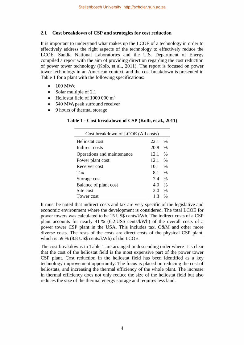
It must be noted that indirect costs and tax are very specific of the legislative and

economic environment where the development is considered. The total LCOE for

power towers was calculated to be 15 US$ cents/kWh. The indirect costs of a CSP

plant accounts for nearly 41 % (6.2 US$ cents/kWh) of the overall costs of a

power tower CSP plant in the USA. This includes tax, O&M and other more

diverse costs. The rests of the costs are direct costs of the physical CSP plant,

which is 59 % (8.8 US$ cents/kWh) of the LCOE.

The cost breakdowns in Table 1 are arranged in descending order where it is clear

that the cost of the heliostat field is the most expensive part of the power tower

CSP plant. Cost reduction in the heliostat field has been identified as a key

technology improvement opportunity. The focus is placed on reducing the cost of

heliostats, and increasing the thermal efficiency of the whole plant. The increase

in thermal efficiency does not only reduce the size of the heliostat field but also

reduces the size of the thermal energy storage and requires less land.


5

Currently the highest efficiency power cycles used in CSP are subcritical water

cycles that have overall thermal efficiencies between 38 and 40 %. Using

advanced power cycles with a higher efficiency (like Helium and supercritical

CO2 cycles) may increase the thermal efficiency to above 50 %. For argument’s

sake, consider a 7 % increase in thermal efficiency from 38 %. This relates to

15.56 % input energy savings. This means that there will be 15.56 % less

heliostats. A 15.56 % saving on heliostats relates to a 3.44 % reduction of the

LCOE based on heliostats and storage alone. However, it is estimated that the use

of an advanced power cycle could provide even greater cost reductions. This is

discussed in detail in section 10.

The key to increased thermal efficiency is to increase the temperature at which

energy is introduced to the power cycle. Apart from the thermodynamic cycle

limitations (discussed in section 2.3) the current operational temperatures of the

storage and heat transfer systems are limited (discussed in sections 2.4 and 2.7).

The argument can be made that an increase of the thermal efficiency is essential to

a reduction in LCOE. This would require higher operational temperatures of the

heat transfer and thermal energy storage system.

2.2 Factors determining thermal efficiency

When considering the overall thermal efficiency of a CSP plant there are many

factors to consider. If thermal energy storage comes into play the energy balance

is more complicated because the storage decouples the receiver from the power

cycle. For argument’s sake, take a simple scenario where the energy absorbed by

the receiver is used directly by the thermodynamic power cycle.

The overall thermal efficiency (ηth(CSP)) is primarily dependent on the thermal

efficiency of the power cycle (ηth), and the thermal efficiency of the receiver

(ηreceiver). Thus,

( ) (2.1)

The thermal efficiency of the power cycle (ηth) can be approximated by the

Chambadal-Novikov efficiency correlation (Novikov, 1958) (Chambadal, 1957):

√

(2.2)

Where TL is the sink temperature, and TH is the source temperature.


6

The thermal efficiency of the receiver is highly dependent on its design, but

generally radiation is the greatest loss in high temperature receivers. The

efficiency of the receiver can be expressed as:

(2.3)

Where is the radiation incident on the receiver, is the solar

radiation absorbed by the receiver and is the thermal losses from the

receiver.:

(2.4)

(2.5)

Here I is the incident radiation, C the concentration ratio of the collector, and A

the surface area of the receiver.

For Qlost it is assumed that the convective losses of the receiver are negligible, and

by applying the Stefan-Boltzmann law:

(2.6)

The following simplifications can be made:

α = 1 and ε = 1 (blackbody)

= 5.670373×10−8

W/m2.K

4

TH = Ts

I = 1000 W/m2

Substituting equations 2.4, 2.5 and 2.6 into equation 2.3, and substituting the

simplified result and equation 2.2 into equation 2.1 yields:

( ) (

) ( √

) (2.7)

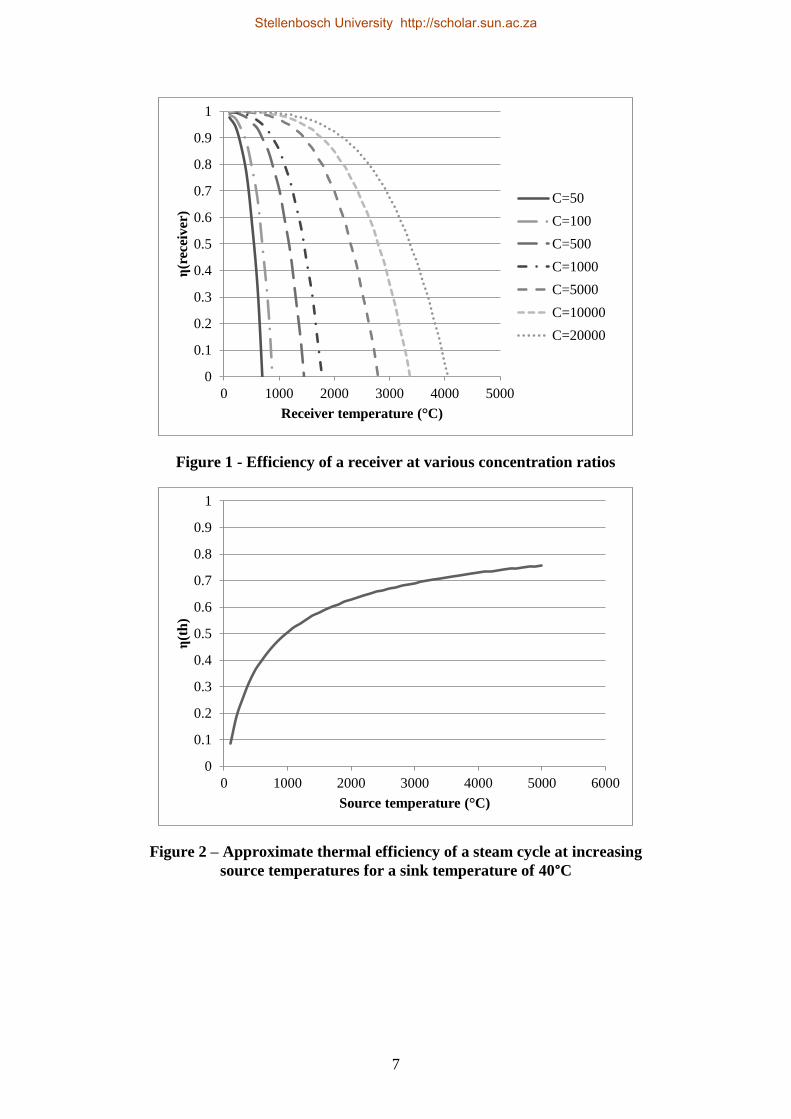
Assuming that the sink temperature is constant at 40°C, Figure 1 and Figure 2

show the efficiency of the receiver and the thermodynamic cycle respectively. The

overall thermal efficiency of the plant is presented in Figure 3, where the overall

thermal efficiency is plotted against receiver temperature for various

concentration ratios.


7

Figure 1 - Efficiency of a receiver at various concentration ratios

Figure 2 – Approximate thermal efficiency of a steam cycle at increasing

source temperatures for a sink temperature of 40°C

0

0.1

0.2

0.3

0.4

0.5

0.6

0.7

0.8

0.9

1

0 1000 2000 3000 4000 5000

η(r

ecei

ver

)

Receiver temperature ( C)

C=50

C=100

C=500

C=1000

C=5000

C=10000

C=20000

0

0.1

0.2

0.3

0.4

0.5

0.6

0.7

0.8

0.9

1

0 1000 2000 3000 4000 5000 6000

η(t

h)

Source temperature ( C)


8

Figure 3 - Thermal efficiency of a CSP plant at different concentration ratios

for a sink temperature of 40°C

For each concentration ratio there is an optimum receiver temperature.

Even though the specifics of any given power plant are distinctly different, this

analysis highlights the following key concepts:

A receiver’s thermal efficiency decreases at elevated temperatures due to

radiation losses.

The larger the surface area of the receiver, the greater the losses (equation

2.6).

Higher source temperature for a thermodynamic power cycle increases the

thermal efficiency of the CSP plant.

Because of these two counteracting effects there is an optimum receiver

temperature for any given concentration ratio.

At higher concentration ratios, radiation losses are less prominent.

Point focus collectors have the highest possible concentration ratio, and

accordingly, the highest possible thermal efficiency. Furthermore, because the

dish concept does not lend it to the use of one central power block, and therefore

the power tower collector is theoretically the CSP concept that has the highest

possible overall thermal efficiency. The higher the maximum flux density of the

receiver, the higher the concentration ratio of the collector will be. Therefore a

high flux density receiver is important in cost reduction; this is discussed in

section 8.

0

0.1

0.2

0.3

0.4

0.5

0.6

0.7

0.8

0.9

1

0 1000 2000 3000 4000 5000

η(r

ecei

ver

)

Source temperature ( C)

C=50

C=100

C=500

C=1000

C=5000

C=10000

C=20000


9

2.3 Power cycles

High efficiency power generation is crucial for the reduction of LCOE. The most

common and versatile power cycle is the steam Rankine cycle. Through years of

development the efficiency of these cycles have improved as the metallurgical

limits of newer, more advanced alloys allow higher temperatures and pressures.

Subcritical steam technology is mature, and power cycles running at live steam

conditions (the steam conditions at the turbine entrance) of 540 °C, 14 MPa are

commonplace. It is possible to obtain thermal efficiencies between 36 and 40 %

with these subcritical power blocks. Most current CSP plants use subcritical steam

power cycles.

Advanced metal alloys have enabled the development of supercritical and ultra-

supercritical power blocks that can achieve thermal efficiencies in the range of 45

to 49 %. Currently there are a number of power plants that are operating at

temperatures above 600 °C, at pressures between 25.5 MPa and 30 MPa, having

practical thermal efficiencies as high as 49 % when cooled with sea water. It has

been shown that these power blocks are not only technically feasible, but also

economical (Bugge, et al., 2006).

In the 1998 the European Union launched a project for the development of ultra-

supercritical steam power plants operating at 700 °C. With the high price of

chrome, the development of high performance austenitic and nickel based alloys

is crucial to the realisation of economic power blocks that can operate above

700 °C (Bugge, et al., 2006).

Air Brayton cycles are under investigation. One of the primary limitations in CSP

is the upper temperature limit of HTFs used in a CSP plant. To overcome this, air

Brayton cycles have been proposed. The overall thermal efficiency of an air

Brayton cycle is not as high as an S-CO2 or a steam cycle, but it can be used in

conjunction with a steam cycle to form a more efficient combined cycle (as a

topping cycle). By using thermal energy storage, the thermal energy of the hot

exhaust gasses of the Brayton cycle can be stored, and then used at night in the

steam cycle. This will also increase the thermal efficiency of the entire cycle

(Allen, et al., 2009).

A number of technical difficulties arise if an air Brayton cycle is applied in CSP.

Because air is a gas, the volume flow rate of the air is high resulting in large

pressure losses in a receiver or an intermediate heat exchanger, and this will have

a significant impact on the thermal efficiency. Furthermore, air is a poor heat

transfer medium and requires large heat exchange surfaces. In normal air Brayton

cycle applications heat is added to the air through combustion. There are

numerous concepts to try and mitigate these issues, but each with drawbacks.

Much work is being done on supercritical CO2 Brayton cycles (S-CO2). Above

500 °C and 20 MPa S-CO2 has properties that enable thermal efficiencies

exceeding 45 % at source temperatures as low as 550°C. Because of the high

density and non-ideal gas properties of S-CO2 it results in exceptionally compact

turbo machinery and heat exchangers. Unfortunately S-CO2 thermodynamic


10

cycles are not well suited for dry cooling, which limits the use of such cycles in

CSP. Another obstacle is the high pressures, but due to metallurgical advances

and the compact nature of S-CO2 power cycles, S-CO2 cycles are considered

technically and economically feasible (Dostal, et al., 2004).

Since supercritical steam, ultra-supercritical steam and S-CO2 power cycles can

utilise higher source temperatures to increase thermal efficiency, higher

temperature TES and HTFs are needed.

2.4 Overview of thermal energy storage and current technical limitations

Thermal energy storage is the main advantage that CSP has over other

renewables. It is important that the thermal energy storage system matches the

operational parameters of the power cycle. Since the goal is to investigate higher

thermal efficiency power cycles, only TES systems that can deliver thermal

energy at temperatures higher than 500°C will be discussed. Currently the two

tank molten nitrate salt system is considered as state of the art and is well suited

for subcritical steam generation, but it is currently at its upper temperature limit

(Gil, et al., 2010).

Thermal energy can be stored in a thermal energy storage material. Thermal

energy storage materials can be either solid or liquid and the storage mechanism

can be classified as either sensible, latent or chemical. In sensible thermal energy

storage the energy is stored by raising the temperature of a material. On the other

hand, latent energy storage refers to thermal storage by adding energy to a

material that is undergoing phase change (this is an isothermal process). This is

illustrated in Figure 4 below. In thermal chemical energy storage the thermal

energy is stored in a reversible chemical reaction.

Sensibl

e

Tem

per

ature

Energy stored

Sensib

le

LatentTemperature of

phase change

Figure 4 - Modes of thermal energy storage

Liquid thermal energy storage media lend themselves to active storage concepts.

In active storage concepts the storage medium is pumped through heat


11

exchangers. In some instances the liquid storage medium is used as HTF in both

the steam generator and the receiver. These are called direct systems. In other TES

systems an intermediate heat transfer fluid is needed to transfer heat from the

receivers to the storage media (known as indirect systems).

Solid thermal energy storage materials generally yield passive storage concepts

where the storage media is contained and heat is added to or taken from the

storage material using a heat transfer fluid. Most latent heat thermal energy

storage and solid sensible concepts are passive, indirect concepts. The

classification is illustrated in Figure 5.

Figure 5 – Classification of TES concepts

Since cost reduction is the greatest factor in CSP, the most important factors for

sensible thermal energy storage are that the storage medium has a large specific

heat, and that the operational temperature of the PCM is as high as possible.

Similarly, for latent heat thermal energy storage, the phase change material

(PCM) needs to have a large heat of fusion. The maximum operational

temperature of the storage system is also extremely important since the storage

temperature is the source temperature of the power cycle.

2.4.1 Current state of the art

Table 2 shows some of the more notable TES systems built for CSP (Medrano, et

al., 2010). There are numerous concepts, some more successful than others.

Notably all of the commercial TES systems are of the active type. The state of the

art is two tank molten salt storage. The specifics of the plant layout depend on the

receiver technology, but the general concept remains the same.

TES

Active

Direct

Indirect

Passive storage system


12

Table 2 - Notable examples of thermal energy storage (Medrano, et al., 2010)

Molten nitrate salt is used as the storage medium and it is held in two tanks, one

hot, and the other cold. The cold tank holds molten nitrate salt at a temperature of

about 230°C. The salt is pumped to either the receiver (direct system, Figure 6)

where the salt is heated up to the salt’s maximum operational temperature, or a

heat exchanger (indirect system, Figure 7). The hot salt is then piped to the hot

tank where it will stay in storage.

For steam generation, hot salt is taken from the hot tank and pumped through

either the steam generator (direct system) or to a heat exchanger (indirect). The

thermal energy of the salt is then used to generate steam, which powers the

turbines. The cooled salt returns to the cold tank.

Storage

media Mode HTF Plant

Collector

type

Operating

temperature

range (°C)

Thermal

capacity

(MWhth)

Total

capacity

(MWe)

Active

Storage

Direct

storageSteam Sensible Steam PS10

Central

recievern.a. 15(50min) 11

Steam Sensible PS20Central

recievern.a. n.a. 20

Oil SensibleMineral Oil

(CALORIA)SEGS I

Parabolic

trough307-240 115 14

Oil SensibleMineral Oil

(ESSO 500)SEGS II

Parabolic

trough316-240 n.a. 30

Molten

saltsSensible Molten salts THEMIS

Central

reciever450-250 40 2.5

Molten

saltsSensible Molten salts Solar Two

Central

reciever565–275 105 10

Molten

saltsSensible Molten salts Gemasolar

Central

reciever565–288 15h 20

Indirect

storageOil Sensible

Mineral Oil

(Santotherm

55)

SSPS DCS

(PSA)

Central

reciever290-180 588 (16 h) 17

Molten

salts,

Rock,

Sand

Sensible Steam Solar oneCentral

reciever304–224 182 10

Molten

saltsSensible Molten salts

SSPS

CESA1

(PSA)

Central

reciever340–220 7 1.2

Molten

saltsSensible Molten salts

SSPS CERS

(PSA)

Central

recievern.a. 2.7 0.5

Molten

saltsSensible Steam

ANDASOL

I

Parabolic

trough381-291 1010 50

Molten

saltsSensible Steam

ANDASOL

II

Parabolic

troughn.a. n.a. 50

Storage concept

Two tanks

One Tank

(Thermocline)

Direct steam

generation

Two tanks


13

Figure 6 - Two tank molten salt TES for central receivers (Direct system)

Figure 7 - Two tank molten salt TES system for parabolic trough (Indirect)

(Herrmann, et al., 2006)

The salts used are typically a binary or a ternary eutectic mixture of nitrate and

nitrite salts. The key issues with molten salt storage are: high melting point

(120 to 240°C), and limited upper operational temperature (565°C).

The properties of various nitrate salts are listed in Table 3. There are three

prominent salt mixtures, Hitec, Hitec XL and Hitec solar salt. Hitec, and Hitec XL

are better suited for parabolic trough applications because of their lower melting


14

points. Hitec solar salt is better suited for use in a central receiver system because

of its higher maximum operational temperature.

The highest storage temperature in commercial thermal energy storage systems a

565°C, and is due to the upper temperature limit of Hitec solar salt. Because of the

temperature limitations on nitrate salts and the risk of solidification, a number of

other thermal energy storage concepts had been proposed and researched. There

are very few of these storage concepts that enable high enough storage

temperatures to enable the use of high thermal efficiency thermodynamic cycles

(Gil, et al., 2010).

Table 3 - Thermal properties of nitrate salts

Unit

Hit

ec X

L

Hit

ec

Hit

ec s

ola

r

salt

Melting point °C 120 142 240

Maximum operating

temperature °C 500 538 567

Density kg/m^3 1640 1762 1794

Specific heat capacity kJ/kg.K 1.9 1.56 1.214

Volumetric heat capacity kJ/m3.K

3116 2748 2177

Viscosity Pa.s 0.0063 0.003 0.0022

Thermal conductivity W/(m.K) na. 0.363 0.536

Prandtl number 12.89 4.98

2.4.2 High temperature storage concepts

Currently there is much research being done on higher temperature thermal energy

storage. Sensible thermal energy storage can use either solid or liquid storage

media. The advantage of a liquid sensible storage medium is that it can be

pumped through a heat exchanger and can be stored in separate hot and cold

tanks. This is a very efficient and elegant form of thermal energy storage. For this

reason the two tank molten salt thermal energy storage is state of the art, and is a

tried and tested system, an important factor when bankability is a foremost

consideration. A number of liquid sensible storage materials have been

investigated in the past (listed in Table 4), but nitrate and nitrite salts have been

found to be the most favourable because of a combination of a manageable

melting point, low cost, high operational temperature and acceptable heat transfer

characteristics.

The current aim is to increase the maximum operational temperature and to

decrease the melting point of salt storage. Thus far a breakthrough has not been

made in a suitable heat transfer salt, and researchers have been investigating other

storage concepts (Gil, et al., 2010).


15

Table 4 - Candidate materials for sensible thermal energy storage (Gil, et al.,

2010)1

Storage

medium Temperature Average

density

(kg/m3)

Thermal

conductivit

y (W/mK)

Heat

capacity

(kJ/

kgK)

Volume

specific

heat

capacity

(kWhth/

m3)

Cost

(US$/

kg)

Cost

(US$/

KWth) Cold

(°C)

Hot

(°C)

Solid

NaCl (solid) 200 500 2160 7 0.85 150 0.15 1

Cast steel 200 700 7800 40 0.6 450 5 60

Cast iron 200 400 7200 37 0.56 160 1 32

Silica fire

bricks 200 700 1820 1.5 1 150 1 7

Magnesia

fire bricks 200

120

0 3000 5 1.15 600 2 6

Sand-rock-

mineral oil 200 300 1700 1 1.3 60 0.15 4.2

Reinforced

concrete 200 400 2200 1.5 0.85 100 0.5 1

Liquid

Mineral Oil 200 300 770 0.12 2.6 55 0.3 4.2

Synthetic

Oil 250 350 900 0.11 2.3 57 3 43

Silicone oil 300 400 900 0.1 2.1 52 5 80

Nitrite salts 250 450 1825 0.57 1.5 152 1 12

Nitrate salts 265 565 1870 0.52 1.6 250 0.5 3.7

Carbonate

salts 450 850 2100 2 1.8 430 2.4 11

Liquid

sodium 270 530 850 71 1.3 80 2 21

Most of the solid TES materials that have been investigated (Table 4) have very

low thermal diffusivity, requiring large heat exchange surfaces. Some of these can

be used in a packed bed, but others need a large heat exchanger that is embedded

in the material. Two notable examples of this are shown in Figure 8 and Figure 9.

These heat transfer modifications make up a significant portion of the capital cost

needed for the thermal energy storage unit and have a significant impact on the

economic viability for these concepts.

Among the various TES materials only PCMs and sensible thermal energy storage

in solids show potential for higher temperature thermal energy storage. Both PCM

and solid sensible TES result in passive storage systems, and this requires HTFs

that can charge and discharge the storage material.

1 Cost was calculated in 2010, and only to be used for comparison.


16

Figure 8 - Graphite heat transfer enhancements for low thermal diffusivity in

PCMs (Tamme, 2007)

Figure 9 - Concrete storage with heat exchanger pipes visible at the end

(Tamme, 2007)

Most research on PCMs and solid sensible TES focussed on lower temperature

storage that is more suited for direct steam solar application (Kenisarin, 2009).

Solid sensible thermal energy storage has been investigated for high temperature

applications, but very few solid storage materials show long term stability through

thermal cycling or prove to be economically viable. Some of the more viable solid

TES materials are shown in Table 4.

Since the temperature of a sensible TES material decreases as it discharges, it is a

technical challenge to design a system that can yield constant thermal output.

Consequently PCMs offer an attractive solution to high temperature TES. PCMs

store thermal energy isothermally, which is significantly easier to design for from

a heat transfer and process control point of view.

Unfortunately isothermal storage has a thermodynamic penalty as it can act as a

large entropy generator (this is discussed in section 8.6.2). To overcome the

shortcomings of PCM storage and solid sensible TES, a combination of both may

be used, or various PCMs can be cascaded to match the heat transfer of the power

cycle.


17

2.5 Thermal energy storage in phase change materials

Thermal energy storage in the latent heat of phase change materials has the

advantage that a great amount of energy can be stored across a small temperature

difference. The higher the heat of fusion of a PCM, the more energy can be stored

in it per unit mass. Therefore a high heat of fusion (λ) is preferable. Other than the

heat of fusion, there are a number of important properties that must be considered

in PCM selection (Kenisarin, 2009):

Melting temperature (Tm)

Low or no sub-cooling

Thermal stability

Chemical stability

Cyclic stability

Thermal conductivity

Specific thermal capacity

Low cost

Availability

Low toxicity

Compatibility with construction materials

The melting temperature of the material is one of the most important

considerations, and it limits the use of the material. The melting point will be the

operational temperature at which the TES system will operate. When designing a

latent TES system, it is important that the melting point of the PCM matches the

input temperature of the power block. Thermodynamically it makes sense to use

multiple PCMs with different melting temperatures in a cascaded fashion to

minimize entropy generation (Michels, et al., 2007). This is discussed in more

detail in section 8.6.2.

Thermal conductivity is probably the most important thermal property other than

heat of fusion and melting temperature. Hoshi, et al. (2005) investigated the

charging and discharging rate between a low conductivity salt and a metallic

phase change material. The results showed that thermal conductivity has a very

large role in the performance of the thermal storage unit. In thermal energy

storage, energy needs to be added and removed from the PCM. Because nearly all

of the feasible PCMs operate between the solid-liquid phase transition, these

storage solutions will be passive thermal storage concepts. Thus, a heat transfer

fluid must transfer thermal energy to and from the heat storage unit (HSU). If the

thermal conductivity of the PCM itself is too low, the size of the heat exchange

surfaces embedded into the PCM will have to be very large or material

modifications will be needed in the PCM (Agyenim, et al., 2009). Most of these

material modifications involve embedding metal or graphite structures into the

PCM to enhance the thermal diffusivity of the bulk material. This might result in

uneconomic storage concepts. If the thermal conductivity of the PCM is high,

sufficient heat transfer rates can be achieved with no material modification or

elaborate heat exchange surfaces.


18

Ideally a PCM should accumulate and release its energy at the same temperature,

but in practice some materials must cool down to substantially lower temperatures

than the melting point before the crystal structure of the material will form in the

absence of crystallization centres. This effect is called subcooling. This is a very

unfavourable phenomenon because energy that has been stored at one temperature

will now be “re-claimed” at a lower temperature. Thus the energy is returned with

more entropy (lower quality).

Naturally the long term stability, safety and general feasibility of the PCM is also

very important. The PCM should not corrode its container, be chemically reactive,

toxic or be a potential fire hazard. It should be chemically stable in its operational

temperature range, and it should be able to go through multiple phase changes

without a change in its thermal properties. This is one of the reasons pure

substances or eutectic mixtures and alloys are considered as candidate PCMs.

2.5.1 Eutectic materials

A eutectic system is a homogeneous mixture of substances that solidifies at a

temperature lower than that of the individual components. The eutectic

composition is the ratio of the constituent substances that has a lower melting

point than any other composition of those substances. The associated melting

temperature is called the eutectic temperature, and the intersection of the eutectic

temperature and the eutectic composition is called the eutectic point. A eutectic

system may comprise of a number of substances, but due to the complexity

associated in investigating these systems, most known eutectic systems are either

binary or ternary. A generic binary eutectic system is shown in Figure 10, where L

denotes liquid phase, α denotes the solid phase of constituent A, and β denotes the

solid phase of constituent B.

A eutectic mixture that is towards the right of the eutectic system is called a

hyper-eutectic composition and to the left is called a hypo-eutectic composition.

As either in a hypo- or hyper-eutectic system, either the α or β phases solidify

first, and cause the material to change phase over a range of temperatures. This

also causes “clumps” of either α or β phase material to form throughout the

material. This causes a non-homogeneous microstructure through the material. In

a eutectic composition, both the α and β phases solidify in a homogeneous manner

with both phases dispersed evenly through the microstructure. The homogeneous

dispersion of the two solid phases aids in material stability, as the “clumps” of α

or β phases in the hypo- and hyper-eutectic compositions have a tendency to drift

out of solution through multiple heating and cooling cycles (Li, et al., 2011).

Thus, eutectic compositions and pure substances are preferred as PCMs because

of thermal stability and very small temperature range for phase change.


19

Figure 10 - Generic phase diagram for a binary eutectic system

2.5.2 Comparison of some PCMs

Through the last three decades the need for thermal energy storage spurred

investigation into various PCMs. Nearly all of the investigated PCMs are binary

and ternary compositions of salts and metals. They can be classified under:

Eutectic salt compositions

Fluorides

Chlorides

Hydroxides

Nitrates

Carbonates

Eutectic metal alloys

To compare the classes of the various PCMs that can be found in literature, a plot

of the heat of fusion against the melting point of each candidate PCM is shown in

Figure 11. The data used in this graph is presented and referenced in Appendix A.

It is clear that the metallic PCMs and fluoride salts have melting temperatures that

are very well suited for high efficiency power blocks.

Generally the thermal conductivity of the salts is extremely low, in the order of

1 W/m2K (Kenisarin, 2009). This is in stark contrast with metal alloys that have

thermal conductivities a factor of more than a hundred higher than those of salts.

This is a very significant factor when it comes to the design of a heat storage unit

(HSU). Hoshi, et al. (2005 ) showed that the thermal conductivity of a PCM is

crucial for charge and discharge rates. The lower the thermal conductivity, the

larger the heat transfer area of the heat exchanger needs to be to achieve adequate

charge and discharge rates. To decrease the size and cost of the heat exchangers,

some researchers attempt to effectively increase the thermal conductivity of the

PCM by modifying the material through the inclusion of high conductivity

conductive elements like graphite flakes (Tamme, et al., 2004).


20

Figure 11 - Comparison of high temperature PCMs found in literature

(Latent heat of fusion against temperature)

Salts have a significant set of drawbacks that metallic PCMs generally do not

exhibit:

Salts are prone to subcooling, where metals generally have no or little

subcooling.

Salts have a large volume change over phase change.

Thus, metallic phase change materials pose a set of significant advantages over

that of salts. Figure 12 shows only the metallic phase change materials that could

be found in literature. Notably, AlSi12, a eutectic alloy of aluminium and silicon

has an exceptionally high heat of fusion, and a fairly moderate melting point. For

this reason, AlSi12 is the only metallic PCM with a melting point over 500 °C that

has been investigated to date (Gil, et al., 2010) (Kenisarin, 2009) (Herrmann, et

al., 2006). Therefore, AlSi12 will be used in this project, even though it will be

pointed out in chapter 10 that a pure aluminium or eutectic silicon-magnesium

alloy is better suited in practice.

AlSi12 is commercially available as LM6 casting alloy, and its metallurgy and

thermal properties are very well known in literature. It is inexpensive, commonly

available and it has a very high thermal conductivity. This makes AlSi12 an ideal

candidate metallic phase change material for both research and commercial

purposes. AlSi12 is discussed in more detail in section 4.1.

0

200

400

600

800

1000

1200

0 200 400 600 800 1000

Late

nt

hea

t of

fusi

on

(J

/g)

Melting temperature ( C)

Carbonates

Chloride eutectic compositions

Hydroxides

Metals

Nitrates

Flouride salts


21

Figure 12 - Metallic phase change materials found in literature (Birchenall, et

al., 1979)

2.6 AlSi12 as a PCM in literature

The first mention of AlSi12 as a PCM was made by Birchenall and Reichmann

(1979) in a paper that proposed thermal energy storage in eutectic metals. The

core of the research was the prediction of the composition, melting temperature

and heat of fusion of eutectic substances by using molecular thermodynamics. In

their text a large list of potential PCMs had been listed. The metallic PCMs that

were listed in their paper are presented in Figure 12. Until recently most research

efforts focussed on TES at temperatures lower than 400 ⁰C due to focus on

parabolic through technology (Kenisarin, 2009). With increased interest in central

receiver technology, the emphasis of storage technology shifted to higher storage

temperatures, making high temperature phase change TES a more relevant field of

research.

Considering PCM research as a whole, a lot of research has gone into the

simulation, testing and modification of low conductivity PCMs. Most of the work

has gone into artificially increasing the thermal conductivity of the PCM material

by including high conductivity material into the bulk of the PCM. These analysis

methods are not of particular importance to metallic PCMs. This will be discussed

in greater detail in chapter 7 (Agyenim, et al., 2009).

The importance of high thermal conductivity is emphasised clearly by Hoshi, et

al. (2005), who compared the effect of thermal conductivity on the discharge rate

of a PCM. In their study they used computational methods to study the discharge

rate of lead and potassium nitrate as PCMs. They found that lead’s inherently high

46.3Mg–53.7Zn

96Zn–4Al Mg(55)–28–17Zn

Al(59)–35Mg–6Zn

Mg(60)–25Cu–15Zn

Mg(52)–25Cu–23Ca

86.4Al–9.4Si–4.2Sb

34.65Mg–65.35Al

60.8Al–33.2Cu–6.0Mg

60.8Al–33.2Cu–6.0Mg

Al(54)–22Cu–18Mg–6Zn

68.5Al–5.0Si–26.5Cu64.3–34.0Cu–1.7Sb

66.92Al–33.08Cu

83.14Al–11.7Si–5.16Mg

87.76Al–12.24Si

Al(65)–30Cu–5Si46.3Al–4.6Si–49.1Cu

Zn2Mg

Zn(49)–45Cu–6Mg

Cu (91)–9P

Cu(69)–17Zn–14P

Cu(74)–19Zn–7Si

Cu(56)–27Si–17Mg

Mg(84)–16CaMg(47)–38Si–15Zn

Cu(80)–20Si

Cu(83)–10P–7Si

Mg2Cu

Si(49)–30Mg–21Ca

Si(56)–44Mg

321.00

0

100

200

300

400

500

600

700

800

0 200 400 600 800 1000

La

ten

t h

eat

of

fusi

on

(J

/g)

Melting temperature ( C)

Al


22

thermal conductivity enabled far higher discharge rates. This comes as no

surprise, but underlines the advantage of using a metallic PCM in thermal energy

storage. Figure 13 shows the results of the analysis done by Hoshi, et al. (2005).

Figure 13 - Analytical comparison of the charging rate of a metallic PCM

versus a salt PCM (Hoshi, et al., 2005 )

Adinberg, Zvegilsky and Epstein (2010) investigated the use of eutectic Zink-Tin

alloy as a PCM in a “heat pipe” type steam generator (shown in Figure 14). The

system was evaluated analytically, and shows that steam could be delivered at

340-360 ⁰C. The applicability of the concept to higher temperatures is limited to

lower temperatures due to the heat transfer arrangement. This concept lends itself

well to direct steam systems due to its operational temperature range.

Figure 14 - Steam generator as proposed by Adinberg et al. (2010)


23

Otherwise there is limited published information on metallic PCMs researched in

CSP. A number of authors have investigated PCM TES concepts for applications

not directly associated to solar.

Burch, et al. (1996) presented a concept where two PCMs are used to store

thermal energy around the catalytic converter in a car’s exhaust system to reduce

light up time and reduce emissions. Figure 15 and Figure 16 shows the physical

setup. The paper does not divulge what PCM is used, but one of the PCMs used in

the prototype is definitely AlSi12 (PCM #1). Figure 17 demonstrates the ability of

the storage unit to keep the catalytic converter warm.

Figure 15 - Thermal storage around a catalyst to reduce the light-up time for

a catalytic converter

Figure 16 - Catalytic converter with PCM TES system


24

Figure 17 - Test results from catalytic converter tests

He and Zhang (2001) investigated a concept intended to capture waste heat from

industrial furnaces for recovery at a later stage. It consists out of a shell and tube

heat exchanger, filled with AlSi12 alloy on the shell side. It has eighteen 20mm

ID tubes running the 400mm length of the heat exchanger. The tubes are

configured in a double pass configuration and air is used as a heat transfer

medium. For the experiment the storage unit is heated up using electrical heating

elements. Figure 18 shows a conceptual drawing of the heat recovery unit, and

Figure 19 shows the temperature readouts of the thermocouples at the positions

indicated in Figure 18 through discharge.

Figure 18 - Waste heat recovery unit using AlSi12 as PCM


25

Figure 19 - Temperature readouts for thermocouples in the storage unit

through discharge

The mass of AlSi12 in the storage unit is not stated explicitly in the paper (just

one of many shortcomings in the paper) making it hard to follow exactly what the

operational parameters of the experiment were. The test is supplemented by a

simulation that does not seem to follow the experimental data particularly well,

nor is it possible to determine exactly where the thermocouples were placed

relative to the heat exchange surfaces.

Wang, et al. (2004) investigated a novel space heater concept (Figure 20). The

idea is to offset electrical usage by charging a mass of AlSi12 as a PCM during

times of the day when electricity is cheaper, and to allow the PCM to bridge the

high cost times of the day through discharge. It consists of a 31 kg block of

AlSi12 alloy encased in insulation with one side open to the atmosphere (Figure

21 and Figure 22). Thermal energy is added to the space heater using long

cartridge heating elements embedded into the PCM.

Figure 20 - Space heater with latent heat storage (Wang, et al., 2004)


26

Figure 21 - Sectioned view of the space heater (Wang, et al., 2004)

Figure 22 - Section through the space heater (Wang, et al., 2004)

The positions of various thermocouples are visible in Figure 22. The heater was

tested and compared against a simple model. The model was simply an energy

balance for the mass of PCM, with appropriate convective heat transfer

coefficients applied to each of its surfaces. The heater was tested at two power

levels, yielding similar results in both cases. The results of one of the tests are

shown in Figure 23. The input power was 1540W and it had a charge time of 8

hours, where it was in latent charge mode for about 3.41 hours. The latent

discharge time was 4.32 hours after the power was switched off. This

demonstrates the phase change material’s ability to charge and discharge

isothermally.


27

Figure 23 - Test results for 1540 W heating power (Wang, et al., 2004)

It must be noted that the corrosive properties of aluminium alloys were not

mentioned in any of the papers dealing with AlSi12 as a storage material. This is

dealt with in section 9.

2.7 Heat transfer fluids and current technical limitations

Since phase change materials lend themselves to passive TES concepts, HTFs

must transfer thermal energy between the receiver, storage and power block. The

three primary HTFs used in CSP are:

Thermal oil

Molten salt

Direct steam

These HTFs have limitations that inhibit CSP plant performance which are

discussed below along with other proposed HTFs that may offer superior heat

transfer performance which will enable the use of high temperature thermal

energy storage. The properties of these HTFs are listed in Table 5 for comparison.


28

Table 5 - Properties of heat transfer fluids

Unit

So

diu

m (

atm

)

NaK

78

(at

m)

Po

tass

ium

Hit

ec X

L

Hit

ec

Hit

ec s

ola

r sa

lt

Do

wth

erm

A

Melting point °C 97.82 -12.6 63.2 120 142 240 15

Maximum

operating

temperature

°C 881.4 785 756.5 500 538 567 400

Density kg/m^3 820 749 715 1640 1762 1794 1056

Specific heat

capacity kJ/kg.K 1.256 0.937 0.782 1.9 1.56 1.214 2.5

Viscosity Pa.s 0.00015 0.00018 0.00017 0.0063 0.003 0.0022 0.0002

Thermal

conductivity W/(m.K) 119.3 26.2 30.7 na. 0.363 0.536 0.093

Prandtl

number 0.0016 0.0063 0.0043 12.89 4.98 5.38

Reference (see

footnotes):

2 2 2 3 3 4 5

2.7.1 Thermal oil6

Some parabolic trough collector (PTC) type solar plants use synthetic oil as a

primary heat transfer fluid. There are various brands of synthetic oil HTFs.

Synthetic heat transfer oils such as Dowtherm A are stable at higher temperatures

than mineral oil. Synthetic oils start to decompose at 400°C. At the maximum

operating temperature the vapour pressure of Dowtherm A is 11 bars, which

means that all the pipes, joints and receiver tubes must be pressurised. Thermal oil

is highly flammable, especially at high temperature. It is also hazardous to the

environment if it should leak out of the system.

2 (Liquid metal engineering center, 1972)

3 (Coastal Chemical, 2012)

4 (Kearney, et al., 2003),

5 (Dow chemical company, 2001)

6 (Dow chemical company, 2001)


29

2.7.2 Molten salt7

Sensible heat storage in molten nitrate salt is one of the most prominent thermal

storage mediums today. The high melting point of eutectic nitrate salts means that

special precautions are needed to prevent freezing. This may be done with either

trace heating or by circulating hot salt through the receiver, which is an energy

loss. Trace heating is where the HTF is heated throughout the system using

heating elements. For this reason it is preferable to use the salt as a primary HTF

in a central receiver system where piping is contained within the tower and the

power block.

Different molten salt mixtures are available but they generally have similar heat

transfer characteristics. The most prominent high temperature salt is known as

solar salt. It is a eutectic mixture of sodium nitrate (60 % by weight) and

potassium nitrate (40 % by weight). It has a melting point of 238°C, and an

operative temperature range of between 260 and 567 °C. It is non-toxic, non-

flammable and has a low vapour pressure.

For lower temperature applications ternary eutectic products like Hitec and Hitec

XL are used. These salt mixtures have melting points of about 100 °C lower than

that of solar salt, but their maximum operational temperature is between 500 and

538°C. These salts are more applicable for parabolic trough collector (PTC)

applications. Table 5 shows the operative temperatures of some molten salts.

Solar salt is better suited for high temperature applications.

There is some incentive to use molten salt as a primary HTF in PTC plants

(Kearney, et al., 2003): Parabolic trough plants represent the most mature CSP

concept; the increased maximum operational temperature (from 400 °C to

450-500°C) means higher thermal efficiency.

The use of molten salt as HTF in a PTC system needs innovative designs to

prevent the solidification of salt in the receiver tubes. The high melting

temperature of molten salt poses a potential reliability issue in CSP installations,

but the risk is substantially mitigated in central receiver plants. The power

consumption of a trace heating system depends on the specific plant, and figures

may vary extensively. In a study done on a 55 MWe PTC system using molten salt

as a primary HTF, the night time thermal power loss of the solar field was

10.7 MWth (Kearney, et al., 2003).

In central receiver plants with molten salt storage it is possible to perform thermal

storage and operate at a maximum temperature of 567 °C. The risk of frozen salt

blockage is still present but because the heat transfer pipes are centralized and

substantially shorter, freeze protection is more manageable.

7 (Coastal Chemical, 2011 ) (Coastal Chemical, 2012)


30

2.7.3 Direct steam

Direct steam allows higher operational temperatures than possible with either

molten salt or thermal oil. Theoretically it is possible to achieve superheated

temperatures, but the high operating pressures are a limiting factor. While it is

possible to build a regular steam cycle running at supercritical pressures, it is a

technical challenge to create receiver equipment that can handle high pressures.

Currently the maximum operational steam conditions for a PTC are 500 °C and

120 bar in an experimental setup at the REAL-DISS test facility at the Endes as

Litoral power plant in Carboneras (Spain). This technology is still in development

but the main challenges are (Eck, et al., 2011):

Availability in large numbers of high pressure components such as flexible

connector hoses and high pressure receiver tubes.

Suitable thermal energy storage

Process management of direct steam generation within a large parallel

field.

In central receiver systems the pressure limitations are far lower, and process

control is much simpler, but thermal storage remains an issue.

Another limiting factor is the trade-off between receiver tube performance and

maximum operating pressure. Higher pressures mean that the receiver tubes must

be made of thicker walled tube. The thicker walls impede the heat transfer

performance of the receiver tubes.

2.7.4 Air or gas

In an attempt to achieve higher thermal efficiencies it has been proposed that

compressed air or gas be used in a Brayton cycle. Since both the HTF and the

working fluid is a gas, the maximum temperature is no longer limited by the HTF

or working fluid. But there are a number of drawbacks:

The low density of the gas/air requires large heat transfer areas for

efficient heat exchange to occur

Since the gas or air is at high pressure, a closed volumetric receiver is

needed. This is a major technical challenge for two reasons; the surface

area needed for effective heat exchange is large, and the aperture needs to

be covered by a completely transparent lens that can withstand high

temperature and pressure (Achenbach, 2011).

Thermal storage is difficult and needs a large surface area for heat

exchange.

One example of proposed CSP concepts using air as a HTF is the SUNSPOT

(Allen, et al., 2009) project.

2.7.5 Sodium

Sodium is a well-known HTF in fast neutron reactors. It has a melting point of

97.8 °C and boiling point of 881.4 °C@atm. It has a very high thermal conductivity


31

and relatively high heat capacity, making it a good HTF, but it is very reactive

with water. In the 1950s the United States of America began the development of

liquid metal fast breeder reactors (LMFBR). Sodium was chosen as the coolant

because of its good heat transfer and nuclear characteristics. The program

outcomes were very stringent and they had to satisfy guidelines and standards that

ensured reliable operation of sodium cooled power plants, and the ability for

operators to live with sodium on a routine basis. All data, guidelines and

experience gained over this program were published in the Sodium-NaK

Engineering Handbook by the Liquid Metals Engineering Centre (Liquid metal

engineering center, 1972)

In the 1980s a consortium funded by the IEA investigated the use of sodium as a

coolant in CSP applications. Testing was done at the Plataforma Solar de Almería

(PSA) as the IEA-SSPS High Flux Experiment (Schiel, 1988). In August 1985 a

sodium fire broke out during a maintenance procedure and caused extensive

damage to the sodium system and the PSA. This event emphasised the importance

of safe liquid metal design practices.

Sodium solidifies at 97.8°C. In a system where the primary source of thermal

energy is intermittent the possibility exists that the sodium could solidify

somewhere in the system. This causes a hazard and some measures will have to be

taken to unblock the system to prevent a sodium spill. This situation is avoided at

all costs in the nuclear industry, and Eutectic NaK alloy is used instead (Liquid

metal engineering center, 1972).

2.7.6 NaK

In LMFBRs that must be operated intermittently, the solidification of sodium

causes an inherent reliability issue. Therefore NaK is used in these reactors

(Liquid metal engineering center, 1972). Similarly one can argue that the use of

sodium in a CSP application causes an inherent risk of blockage since the energy

source is intermittent, thus NaK is more suitable for CSP applications.

NaK is a eutectic alloy of sodium and potassium that melts at -12.8°C@ atm and

boils at 785°@ atm. It has heat transfer properties inferior to those of sodium (see

Table 5), and a relatively low specific heat capacity compared to other HTFs, but

it is still considered an excellent heat transfer medium. The NaK eutectic system

(shown in Figure 24) also allows for different compositions of sodium and

potassium. Eutectic NaK has composition of 77.8 % potassium by weight and

22.2 % sodium. It is possible to use NaK46 (46 % potassium), which has a

melting point of 20 °C, and has higher thermal conductivity and greater specific

heat capacity than eutectic NaK (Liquid metal engineering center, 1972). The

properties of sodium, potassium and NaK are shown in Table 5. The properties for

NaK (in Table 5) is that of eutectic NaK alloy, even though it is acknowledged

that NaK alloy with higher sodium content is better suited for CSP applications

because of its superior heat transfer characteristics and acceptable melting point.


32

Figure 24 - Sodium-Potassium eutectic system (Liquid metal engineering

center, 1972)

The biggest risk involving NaK and sodium is that they react violently with water.

This becomes a problem during routine maintenance and when parts need to be

replaced. In a system using NaK it is possible to clear the piping using high

pressure inert gas when the system has cooled down. This is inherently safer than

a situation where there is a risk of pipe blockage during maintenance.

By pressurising eutectic NaK to a pressure of 10 bar, the operational temperature

of liquid NaK can be increased to over 1100 °C (Liquid metal engineering center,

1972).

2.7.7 Conclusion

Considering all the current HTF solutions in CSP, limitations on the maximum

operational temperature is the most prominent. Liquid metals pose an elegant but

risky solution to the problem, capable of maximum operational temperatures

between 785 °C (NaK) and 881 °C (Sodium) at atmospheric pressure, which can

be increased to temperatures exceeding 1100 °C with moderate pressurisation. A

comparison between the temperature ranges of the HTFs is shown in Figure 25.

Note that pressurised NaK46 has an operational temperature range exceeding all

of the other HTFs.

Both NaK and sodium are highly reactive with water, and both pose a serious

safety risk. Experience with NaK and sodium as HTFs in LMFBRs yielded an

extensive database of regulations, design codes and handling instructions that can

be used to create a safe design that use either NaK or sodium as an HTF.

Furthermore, NaK’s low melting point is more suited for use in CSP than sodium

because it does not pose an inherent risk for pipe blockage. Accordingly, it is

possible to design a CSP system where personnel can work with the NaK system

without danger, and have the advantage of high operating temperatures. The fact


33

that NaK needs no freeze protection means that the entire primary loop can be

shut down at night with no risk of damage to the receiver, pumps or heat

exchangers. This means that the primary heat transfer system can be designed to

be much more robust.

It should also be noted that other NaK compositions can also be used to increase

the thermal conductivity, maximum operative temperature and to increase the

specific heat capacity. By using a NaK composition of 48 % potassium by weight,

the NaK alloy still melts at 20 °C but the heat transfer properties are improved.

This translates to savings in pumping power for the primary cooling loop.

Because all literature on NaK is based on the eutectic composition, the eutectic

composition will be considered from here on unless otherwise specified. The

properties of NaK will be discussed in more detail in section 4.2.

Figure 25 - Comparison of HTF operative temperatures

2.8 Conclusion and project scope

Currently the main objective for research and development in CSP is the reduction

of LCOE. One of the most direct paths to cost reduction is to increase the thermal

efficiency of the power block. This requires a higher source temperature than

possible with two-tank molten salt storage. Unfortunately the maximum storage

temperatures of molten salts are limited to 565 ⁰C. It is possible to store thermal

energy isothermally at higher temperatures in PCMs. The operational temperature

of a PCM is its melting temperature, and at temperatures higher than 565 ⁰C only

fluoride salts, chloride salts and eutectic metal alloys can be used. Metallic PCMs

have properties that make them a more viable class of storage material than salt

based PCMs.

-100 0 100 200 300 400 500 600 700 800 900 1000

Hitec XL

Hitec

Hitec Solar Salt

Thermal oil

NaK78 (atm)

NaK46 (10bar)

Sodium (atm)

Water

Operational Temperature - C


34

Looking at the known metallic PCMs, there is a number of pure metals and

eutectic metal alloy that are suitable characteristics for high temperature TES.

AlSi12 has an exceptionally high heat of fusion at a reasonably manageable

melting temperature, making it an ideal candidate metallic PCM for research

purposes. Furthermore it is affordable, readily available and has very favourable

thermophysical properties.

Because thermal energy storage in PCMs result in passive storage concepts, a heat

transfer fluid is needed that can operate at temperatures exceeding that of metallic

PCMs. Considering all available HTFs, NaK is the heat transfer fluid best suited

for CSP applications due to its low melting point (-12.8 ⁰C), high boiling point,

low vapour pressure and high thermal conductivity.

The scope of this project is limited to:

The development of a TES concept that utilizes metallic PCMs to

demonstrate the implementation of advanced power cycles.

Explore and evaluate the appropriate analytical tools necessary for

evaluation of metallic PCM TES systems and metallic HTFs.

Build a prototype to evaluate the concept and analytical tools that may be

used for design.

Use these analytical tools to prove the concept and to determine

operational parameters.

Perform a techno-economic feasibility study and highlight the role of

metallic PCMs as a method to LCOE reduction.

Determine what future research is required for further development of

these storage concepts.


35

3 THERMAL ENERGY STORAGE CONCEPT

In chapter 2 it has been established that metallic PCMs will enable the use of

higher efficiency power cycles through high temperature storage. The specific

PCM used depends on the application and the melting point of the PCM. This is

primarily a techno-economic consideration and is discussed in chapter 10. AlSi12

is a metallic PCM which has been identified as a good PCM with a high heat of

fusion, high thermal conductivity and a reasonably high melting point. It is readily

available and is inexpensive which makes AlSi12 an excellent candidate PCM for

this project. Furthermore, NaK has been identified as an ideal HTF for high

temperature applications. AlSi12 melts at 577°C, and is well suited for a

subcritical steam cycle. The concept will be developed to apply AlSi12 to a

subcritical steam cycle, but it must be kept in mind that the concepts are also

applicable for higher temperature storage.

NaK is extremely reactive with water, and has serious safety implications. In the

nuclear industry NaK-water steam generators are common, but the application of

liquid metal cooling in CSP is still under development and the feasibility of a

NaK-water steam generator in CSP is still not clear. Consequently, two storage

concepts are developed. The one is called the direct steam generator (DSG)

concept, where the steam is generated directly from the PCM (section 3.1). The

key here is to separate the NAK and water heat exchangers from each other using

the PCM as a buffer. The other is the indirect steam generator (ISG) concept

(section 3.2) where the steam is generated in a steam generator separate from the

storage unit like in a nuclear power plant.

Each of these concepts has to be evaluated using a preliminary design that is

representative of what might be a real world implementation. For AlSi12, a

subcritical steam cycle is the most applicable power cycle, and the concepts are

developed accordingly. This is discussed in greater detail in chapter 8. The two

concepts are presented in the subsequent sections along with a power cycle in

which it is implemented.

The power cycle is specified as follows:

100 MW electrical output;

Base load operation;

540 °C, 140 bar superheat;

540 °C, 30 bar re-heat;

one open-feed water heater supplied from the high-pressure turbine outlet;

and

air-cooled condenser.

3.1 Direct steam generator

In the direct steam generator, both the steam pipes and the liquid metal heat

transfer pipes are imbedded into the bulk of the storage media as illustrated in

Figure 26. Heat is added to the PCM using the liquid metal heat exchanger, and


36

heat is removed using the water/steam heat exchanger. As illustrated in Figure 26,

the water/steam and liquid metal heat transfer pipes are arranged regularly through

the whole melt. Therefore, steam is generated with heat directly from the PCM.

As the PCM charges and discharges, the PCM will melt or solidify in a radial

fashion around the pipes of the heat exchangers. This is discussed in more detail

in chapter 7.

NaK in:

NaK out:

Steam

out

Steam

in

AlSi12 PCM

Figure 26 - Direct steam generator concept

In a subcritical steam power cycle three heat exchangers are needed:

Boiler

Super-heater

Re-heater

All three parts of the steam generation system are conceptually the same as in

Figure 26. The layout of the subcritical power cycle is shown in Figure 27. The

boundary conditions of these subsections of the steam generator are presented in

section 8.1.

The specifications and boundary conditions of the liquid metal heat exchanger in

the storage system is determined by nature of the field, the location of the plant

and the capabilities of the receiver. This is discussed in section 8.2


37

LP-Turbine

G

HP-Turbine

CondenserO-FWH FW Pump

FW Pump

Superheater

Boiler

Re-heater

Steam drum

NaK to storage

NaK to Recievers

Collector field

Figure 27 - Power cycle with the direct steam generation concept

3.2 Indirect steam generator

In the ISG concept, only NaK heat transfer pipes will be imbedded into the PCM

as illustrated in Figure 28. A separate steam generator will be used, and the plant

layout is shown in Figure 29 where it can be seen that the steam generator is

separate from the storage unit. Because the PCM charges and discharges

isothermally, the NaK will always exit the storage system at a temperature close

to the melting point of the PCM whether it is charging or discharging.

In this case the steam generator is a separate and specially built unit that is beyond

the scope of this project. Similarly to the DSG concept, the sizing of the liquid

metal heat exchanger in the heat storage unit is primarily dictated by the factors

affecting the energy input into the storage system. This is discussed in section 8.2

During charging, NaK passes from the receivers, through the storage system and

to the steam generator and then back to the receivers. During discharge the

receivers will be bypassed, and the NaK will only cycle between the steam

generator and the storage unit.

Similarly to the DSG concept the PCM will melt or solidify in a radial fashion

around the pipes of the heat exchangers. This is discussed in more detail in

chapter 7.


38

NaK in:

NaK out:

AlSi12 PCM

Figure 28 - Indirect steam generation concept

LP- Turbine

G

HP- Turbine

CondenserO- FWH FW Pump

FW Pump

NaK to storage

NaK to RecieversCollector field

Boiler

Super heater

Re-heater

Metallic PCM

Storage

Figure 29 - Power cycle with the indirect steam generation concept

NaK to steam generator


39

4 MATERIAL PROPERTIES

4.1 The properties and characteristics of AlSi12

Eutectic Aluminium Silicon alloy is well known for having a high heat of fusion,

low melting point, high fluidity, low thermal expansion coefficient and low

shrinkage during solidification. For this reason it is popular in the casting industry

for the production of cast parts with thin sections and work pieces with fine detail.

AlSi12 is known in the casting industry by many names depending on region, but

in the commonwealth it is known by its British standards designation: LM6. The

composition of LM6 is standardised in the BS 1490:1988 LM6 standard, and can

be regularly purchased as a master alloy. The composition of LM6 is listed in

Table 6.

Table 6 - Composition specifications of LM6 alloy (BS 1490:1988 LM6)

Element wt.%

Copper 0.1 max

Magnesium 0.10 max

Silicon 10.0-13.0

Iron 0.6 max

Manganese 0.5 max

Nickel 0.1 max

Zink 0.1 max

Lead 0.1 max

Tin 0.05 max

Titanium 0.2 max

Aluminium Remainder

The phase diagram of the Al-Si eutectic system is shown in Figure 30 on the next

page. One thing to notice is that it is a very simple phase system. It only has two

solid solution phases, a face cantered cubic aluminium α-phase, and a diamond

cubic silicon β-phase. These phases crystallize out of solution in hyper- and hypo-

eutectic solutions affecting the microstructure of the alloy. The effect of the

microstructure might have effects on the cyclic stability of the alloy. This is

discussed later in this section.

At the eutectic point (12.2 at.% silicon) the phase change occurs at 577 ⁰C. Master

alloys are manufactured within specifications will be close to the eutectic point,

but will still have α- and β-phase inclusions depending on the exact composition.


40

Figure 30 - Aluminium-Silicon eutectic system (Murray, et al., 1984)

4.1.1 Thermal and physical properties of eutectic Aluminium silicon alloy

To perform thermal analysis, sizing and mechanical design, knowledge of the

thermophysical properties of AlSi12 is important. Because AlSi12 is just one of a

large family of alloys, the exact properties of AlSi12 are not as commonly

available as one would expect. Various manufacturers do in-house testing for the

required properties. This data is considered a company asset and is not divulged

into the public domain. This means that there is no central database for AlSi12

properties over a large range of temperatures like there is for water and NaK.

Because the nature of this work is to evaluate the feasibility of using metallic

PCMs as high temperature thermal storage materials, detailed high temperature

materials testing on AlSi12 is not possible due to the high costs associated with it.

Only some of the most critical properties like heat of fusion and melting

temperature will be measured using a Scanning Differential Calorimeter (DSC).

The required accuracy of the properties depends on the application. Because the

storage system will operate around the melting point of the system, it is important

that the properties are representative of AlSi12 around the melting point in either

the solid or liquid state.

The general properties of eutectic AlSi12 are presented in Table 7 as quoted on an

online materials database. The temperature range of these properties was not

listed.


41

Table 7 - General material properties of eutectic AlSi12 alloy (Matbase)

Mechanical properties

Solidification shrinkage 0.5 %

Density 2650 kg/m2

Fatigue failure 55-60 MPa

Shear modulus 27500-28000 MPa

Tensile strength 150 MPa

Yield strength 70 MPa

Young's modulus 72000-75000 MPa

Thermal properties

Melting temperature 577 degC

Specific heat 970 J/kg.K

Thermal conductivity 130-190 W/m.K

Thermal expansion 21 e-6/K

Heat of fusion 460 kJ/kg

To date a limited number of authors have published on the practical use of AlSi12

as a PCM (see section 2.6), and because of this, their analytical work had to be

based on some assumptions. Both of the authors who did a practical investigation

into AlSi12 as a PCM did not reference the property set that they used. He et al.

used the following values (Table 8):

Table 8 - Thermal properties used by He et al. (He, et al., 2001)


Density 2661 kg/m2

Thermal properties


Specific heat 939 J/kg.K

Latent heat of fusion 515 kJ/kg

Curiously, the thermal conductivity of the material is not mentioned in the paper,

which is a very important factor in modelling PCM systems.

Wang et al. (Wang, et al., 2004) used the values presented in Table 9:

Table 9 - Thermophysical properties of AlSi12 as used by Wang et al.


Density 2700 kg/m2

Thermal properties


Specific heat (solid) 1038 J/kg.K

Specific heat (liquid) 1741 J/kg.K

Thermal conductivity 160 W/m.K



42

Since there is some inconsistency between the values found in literature (Wang, et

al., 2004) (He, et al., 2001) other sources had to be used. The values for specific

heat and heat of fusion stated by Wang et al. are considered correct because they

were measured using a differential scanning calorimeter. The rest of the values

used in this text have been taken from a selection of text books and were

recommended by a metallurgist specializing in aluminium alloys (Munn, 2013).

Unfortunately the values of thermal conductivity for liquid AlSi12 could not be

found, and the value for solid AlSi12 around the melting point is used as

recommended by a metallurgist (Munn, 2013). The physical properties used in

this text are presented in Table 10.

Table 10 - Properties of AlSi12

Mechanical properties Temperature Reference

Solidification

shrinkage

0.5 % n.a. (Matbase) (Mondolfo,

1976)

Thermal expansion

(solid)

21.6 10-6

m/m.K

27-327°C (Mondolfo, 1976)

Thermal expansion

(liquid)

10

(Mondolfo, 1976)

Dynamic Viscosity 2.96 mPa.s 577°C-580°C (Brandes, et al., 1998)

Density 2560 kg/m3 577°C (Mondolfo, 1976)

Thermal properties

Melting temperature 577 degC n.a. Measured & (Mondolfo,

1976)

Specific heat (solid) 1038 J/kg.K 577°C (Wang, et al., 2004)

Specific heat (liquid) 1741 J/kg.K 577°C (Wang, et al., 2004)

Thermal conductivity 160 W/m.K 577°C (Wang, et al., 2004) &

(Mondolfo, 1976)

(Tenekedjiev, et al., 1995)

Heat of fusion 560 kJ/kg n.a. Measured

4.2 The properties and characteristics of NaK

In section 2.7 it has been established that NaK is an ideal heat transfer fluid for

high temperature CSP applications. It has distinct advantages and shares some

heat transfer properties with potassium and sodium that make high heat transfer

rates possible at temperatures not possible with other HTFs, whilst not requiring

trace heating due to its low melting point. It has two drawbacks: the first being

that, it has a relatively low specific heat; and the second, but most important

drawback is that it is extremely reactive with water.

Because sodium and NaK are difficult materials to work with the Liquid Metals

Engineering Centre summarised all data on Sodium and NaK in the Sodium-NaK

Engineering Handbook. This is the most comprehensive resource on liquid metal

engineering.


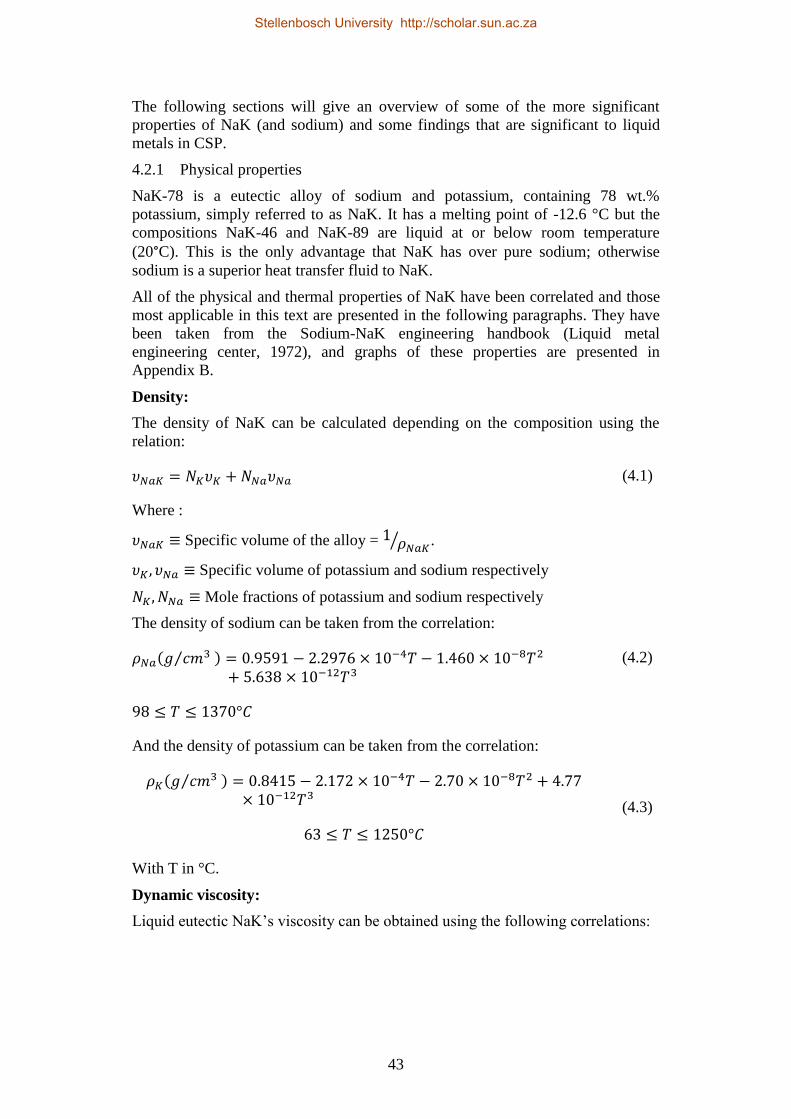
43

The following sections will give an overview of some of the more significant

properties of NaK (and sodium) and some findings that are significant to liquid

metals in CSP.

4.2.1 Physical properties

NaK-78 is a eutectic alloy of sodium and potassium, containing 78 wt.%

potassium, simply referred to as NaK. It has a melting point of -12.6 °C but the

compositions NaK-46 and NaK-89 are liquid at or below room temperature

(20°C). This is the only advantage that NaK has over pure sodium; otherwise

sodium is a superior heat transfer fluid to NaK.

All of the physical and thermal properties of NaK have been correlated and those

most applicable in this text are presented in the following paragraphs. They have

been taken from the Sodium-NaK engineering handbook (Liquid metal

engineering center, 1972), and graphs of these properties are presented in

Appendix B.

Density:

The density of NaK can be calculated depending on the composition using the

relation:

(4.1)

Where :

Specific volume of the alloy = ⁄ .

Specific volume of potassium and sodium respectively

Mole fractions of potassium and sodium respectively

The density of sodium can be taken from the correlation:

( ⁄ )

(4.2)

And the density of potassium can be taken from the correlation:

( ⁄ )

(4.3)

With T in °C.

Dynamic viscosity:

Liquid eutectic NaK’s viscosity can be obtained using the following correlations:


44

( )

[

]

(4.4)

( )

[

]

(4.5)

Where μ is measured in centipoise, ρ in g/cm3 and T in K.

Thermal conductivity:

The thermal conductivity of eutectic NaK can be taken from the correlation:

( )

(4.6)

With T in °C.

Specific heat:

The specific heat of eutectic NaK can be calculated from the correlation:\

( )

(4.7)

With T in °C.

The specific heat of eutectic NaK is presented in Figure 99 as a function of

temperature (presented in SI units)

The thermal diffusivity and Prandtl number of eutectic NaK are presented in

Figure 31 and Figure 32 respectively to give quick reference in subsequent

subsections


45

Figure 31 - Thermal diffusivity of eutectic NaK

Figure 32 - Prandtl number of eutectic NaK

2.50E-05

3.00E-05

3.50E-05

4.00E-05

100 200 300 400 500 600 700 800

Th

erm

al d

iffu

siv

ity

(m

2/s

)

Temperature (⁰C)

0

0.005

0.01

0.015

0.02

0.025

100 200 300 400 500 600 700 800

Pra

nd

tl n

um

ber

Temperature (⁰C)


46

4.2.2 Safety

One of the key issues when it comes to liquid metals is safety. Throughout the

liquid metal heat transfer programmes, a key consideration was to establish

design, handling and operational protocols to allow engineers, technicians and

operators to work with liquid metals on a routine basis in a safe manner.

Unlike lead-bismuth and mercury, sodium and NaK are not toxic, but the most

prominent concerns are:

Corrosion

Leakage (from pumps and valves)

Maintenance procedures

Of which the major issue underpinning all of these is a fire hazard. Alkali metals

react exothermically with water, producing hydrogen, and forming a strong base.

It can be described with the following equation:

(4.8)

And

(4.9)

Where sodium hydroxide is a very strong base and the hydrogen burns off during

the reaction. Sodium and potassium’s affinity for water is so strong, that the

reaction can occur with the moisture from the air. If NaK is exposed to air, a

yellow potassium superoxide is formed, that reacts explosively with organic

compounds. Thus, NaK should be kept away from air and water at all times. In

practice NaK is stored under dry argon or nitrogen.

In the mid-1980s the IEA – SSPS High flux experiment investigated the

performance of a sodium cooled receiver (discussed in section 8.2.2). During a

maintenance procedure, technicians had to remove a pipe which was blocked with

solidified sodium. A section that was mistaken to be solidified actually contained

a vacuum which made it appear to be cool and when the pipe was removed, liquid

sodium leaked out of the system. The moisture in the air started a fire that

destroyed the facility. This could have prevented if proper design protocol was

followed.

The Sodium-NaK engineering handbook stipulates all factors of liquid metal

engineering, and addresses all matters from handling to equipment design.

Following these established guidelines, it is possible to build a heat transfer

system that is safe and reliable, offering superior heat transfer solutions for CSP

applications.

An intermittent power input is a key reliability issue in CSP. Nitrate salts must be

kept in a molten state throughout the night and during maintenance. Trace heating

is used to keep pipes warm at night and during down time and the molten salt

must be continually pumped through these pipes to prevent solidification in cold


47

spots like the receiver. A similar situation would exist if sodium is used, and this

would present a significant safety risk during maintenance.

For this reason NaK’s low melting point has two advantages. The first is that there

is no need for trace heating, and secondly, maintenance and repairs can be done in

a safe manner, because it is possible to purge the pipes and equipment at room

temperature. This is the reason NaK is used in experimental LMFBRs.

A convenient attribute of NaK is that it is electrically conductive, making

electromagnetic pumping possible. This further adds to safety, as the seals on a

conventional pump is a great concern.

4.2.3 Steam generator design

Because NaK’s great reactivity with water, the steam generator is a great safety

concern. For the success of any CSP plant, the risk to the investor needs to be

minimized and proven through demonstration. If NaK is to be implemented into a

CSP plant, one of the main concerns would be that of a NaK steam generator,

where NaK and water would come into close proximity with each other. This

requires that the heat exchangers should have a high structural integrity and be

capable of handling the worst possible accidents.

The high heat transfer capability of NaK means that the heat exchanger will

experience high thermal stresses during transient conditions. In the past sodium

heated steam generators have failed due to thermal stress, and lessons learnt from

these failures have been used to establish design guidelines to ensure safe and

reliable designs in the future. Some of these problems include:

Tube-to-tube-sheet joints

Differential expansion

Flow distribution

Vibration

Thermal transient stress

Other issues like corrosion from the water side and material compatibility are

some design aspects that had to be resolved. NaK/sodium is not as corrosive as

lead-bismuth, and proper material selection is sufficient to ensure lasting

corrosion protection in the steam generator as well as the whole system from the

NaK side. The central material related issues that must be taken into account can

be summarised as:

Material compatibility

Corrosion

Erosion

Material processes

Throughout the life of the steam generator, some key issues must be addressed.

These might be the hardest to implement, because of human error. For this reason

a certain level of robustness must be designed into the steam generator. Some of

the more prominent problems that must be considered are:


48

Flow misdistribution

Excessive thermal transients

Feed water purity

Sodium purity

Through years of experience and a number of failures, the design criteria for

NaK/sodium steam generators have been built up to design for all of these

problems. Along with good design protocol, leak detection systems enable the

plant to stop and clear the steam generator in the event of a leak. Generally this

involves the detection of hydrogen, and then clearing the heat exchanger using

high pressure inert gas. In the nuclear industry double redundancy is a

requirement, but other techniques of risk dissipation can be implemented in CSP,

since the field can be defocused in the event of an emergency.

A number of successful experimental and commercial LMFBRs has been built

and is still in use to this day proving the technical viability of NaK and sodium

heated steam generators. The only factor that may prohibit the use of such a steam

generator may be cost, and a detailed economic feasibility study may shed some

light on the implications on LCOE.

4.3 Other materials

Some of the more standard materials used in this project include:

Water

Stainless steel

Mild steel

The properties of water are taken form the IAPWS industrial formulation 1997 for

the thermodynamic properties of water and steam (Wagner, et al., 2011). This is

known to be the most comprehensive and accurate model for water and steam

properties.

The construction material of choice for the experimental rig is low carbon steel,

and the material proposed for use for the NaK heat exchanger is austenitic

stainless steel as prescribed for the use in the Liquid metals engineering handbook

(Liquid metal engineering center, 1972). The thermal properties presented in

Table 11 are used throughout this text.

Table 11 – Thermal properties of low carbon steel and stainless steel 304

Low carbon steel

Stainless steel

(AISI 304)

Density (kg/m3) 7854 7900

Specific heat (J/kg.K) 685 482

Thermal conductivity (W/m.K) 36.2 22.6

Thermal expansion (10-6

m/m.K) 16.6 18.7


49

5 FLOWNEX

The simulation and modelling will be done in Flownex® SE throughout this

project. Flownex® is a simulation environment that has been developed and

validated within an ISO 9001 and ASME NQA1 accredited system and has seen

extensive validation and verification within these systems. Flownex has also been

validated in the nuclear industry, and holds the following accreditations:

In 2007 the National Nuclear Regulator (NNR) of South Africa reviewed

the Flownex® Software Verification & Validation (V&V) status and

found it to be acceptable to be used to support the design and safety case

for the PBMR.

NQA1:2008 (Westinghouse EC USA)

2009: ISO 9001 (audited and approved)

Flownex uses nodes connected by components to analyse thermal-fluid networks.

Each component is a mathematical model; mostly comprising partial differential

equations (PDE) for mass, momentum and energy conservation. Flownex solves

these networks of PDEs to yield the temperature, pressure and mass flow rates

through the network. These networks can either be solved as steady state or

transient state problems. Additional equations are also solved to describe other

aspects such as shaft dynamics, electrical networks and control systems. The

solution procedure is well documented in the Flownex theory help files supplied

with the program. The Flownex model of a Rankine cycle is shown in Figure 33.

Figure 33 – Flownex model of a Rankine cycle

Flownex can deal with single and multiphase flow, and has built-in heat transfer

and pressure drop correlations which are automatically chosen to yield the most

accurate results possible. It is also possible to manually program new correlations

into Flownex using a C# user interface.

An extensive component, fluid and material database makes it possible to build up

network models of varying complexity. It is also possible to add components,

fluids and materials to the database using a specialized tool set. The database is


50

well documented and enables the user to evaluate every component and determine

the applicability of the results.

A number of built-in tools in the Flownex package proved to be very helpful in

this project. The design and optimization tools were key to the sizing of heat

exchangers and the sensitivity analysis tool helped with the discretization of the

heat transfer and flow problems.


51

6 HEAT TRANSFER MECHANISMS

To evaluate and establish design guidelines, heat transfer predictions for the heat

exchangers are needed. Both liquid metal heat transfer and forced convective

boiling are considered specialist fields of heat transfer, and the methods used in

this text are described here.

6.1 Liquid metal heat transfer8

Liquid metals have unique thermal properties that make them very efficient HTFs.

Low viscosity and high thermal conductivity means that NaK and sodium have

very low Prandtl numbers as discussed in section 4.2. This means that conductive

heat transfer is dominant. For this reason, extremely high flux densities can be

achieved in a NaK heat exchanger, this is especially important in the receiver,

where it leads to a smaller heat exchanger, and higher overall efficiency. Because

of the application of NaK in this study, only single phase heat transfer in tubes

will be dealt with.

A property of heavy metals such as lead-bismuth and mercury is that they tend not

to properly wet iron and iron alloy surfaces because of thin layers of oxides that

form. This is only of concern with NaK in the presence of an abundance of gasses

in the system. Otherwise there is enough reason to assume perfect wetting

between NaK and the heat exchange surfaces and that there is no contact

resistance that have to be considered.

In the case of normal liquids in forced convective heat transfer, the greatest

temperature variation is found in the laminar sub-layer at the channel wall, where

molecular thermal conduction is the primary mode of heat transfer in this layer. In

the turbulent core of the tube eddy conduction is the primary heat transfer mode.

In stark contrast, the thermal conductivity in liquid metals is so high that

molecular thermal conductivity is competing with eddy conductivity in the

turbulent core. The result is that it is possible to get very high heat transfer rates

into the fluid without boiling.

According to the Sodium-NaK engineering handbook, the recommended heat

transfer correlations:

(6.1)

for uniform heat flux, and

(6.2)

for uniform wall temperature. Pe is the Péclet number, which is the product of the

Reynolds and the Prandtl numbers. These correlations are accurate for



52

6.2 Convective boiling heat transfer inside plain tubes

Convective boiling yields extremely high heat transfer rates, but it is difficult to

predict the local heat transfer coefficients for a fluid flowing within a pipe because

of the complex hydrodynamic behaviour of a two phase fluid. A number of

correlations have been developed to predict heat transfer and pressure drop of an

evaporating fluid in a closed channel. Generally these correlations have limited

accuracy, but some perform better than others depending on application.

All of these correlations assume a homogeneous model. In the homogeneous

model, the fluid properties of the fluid at any given position of the pipe are taken

as a weighted average between the properties of the liquid and gaseous phases.

The gas-liquid composition (otherwise known as the steam quality, and

represented by x) is predicted by the model itself.

The local two phase flow boiling heat transfer coefficient (αtp) is defined as:

( ) (6.3)

Where is the local heat flux from the tube wall into the fluid, Tsat is the local

saturation pressure, and Twall is the local, uniform wall temperature along the

evaporator tube.

There are two mechanisms at work with forced convective boiling:

Nucleate boiling heat transfer (αnb)

Convective boiling heat transfer (αcb)

Using a power law format, the flow boiling heat transfer can be expressed as:

[( ) ( )

] (6.4)

Most of the models use this expression as a basis, and use various methods to

predict the nucleate and convective boiling heat transfer. Nucleate boiling heat

transfer (αnb) is considered to be a function of heat flux and convective boiling

heat transfer (αcb) is considered to be a function of mass velocity. This is an

important factor that needs consideration for process control.

There are many correlations, but the two recommended heat transfer correlations

for flow boiling are the Steiner-Taborek asymptotic model (Steiner, et al., 1992)

for vertical tubes, and the updated version of the Kattan-Thome-Favrat model

(Thome, et al., 2002) for horizontal tubes. Only vertical tubes will be considered

in this text due to the geometry of the concept. The models were incorporated into

the Flownex heat transfer models discussed in chapter 8.


53

7 MOVING BOUNDARY HEAT TRASNFER AROUND VERTICAL

HEAT TRANSFER TUBES

As shown in chapter 3, the heat storage unit concept consists of heat transfer tubes

embedded at regular intervals throughout a pool of phase change materials

(PCM). There are two variations of the concept, the indirect steam generation

(ISG) and the direct steam generation (DSG).

In the DSG concept the liquid metal heat transfer pipes (heat input) and the

steam/water heat transfer pipes (heat output) are all embedded at regular intervals

throughout the melt. This may lead to a very complex thermal distribution

throughout the PCM which is highly dependent on the exact geometry of both the

liquid metal and the steam/water heat exchange pipes. To simplify the analysis,

only discharge conditions will be considered for the DSG concept, since a

computational fluid dynamics (CFD) solution is necessary for charge conditions.

On the other hand, in the ISG concept, the same heat exchange surface is used to

charge and discharge the heat storage unit (HSU), resulting in a fairly simple heat

transfer problem from a geometrical point of view.

Axial conduction is ignored to simplify the heat transfer problem. If there is a

significant temperature gradient along the length of a heat transfer pipe, the

chances are that the cylinder will not grow out evenly along the length of the pipe,

but like a cone. This phenomenon must be analysed using a CFD analysis, and it

is outside the scope of this project. The assumption makes this a one dimensional

heat transfer problem around each heat transfer pipe.

For simplification, the entire volume of PCM is discretized into hexagonal

cylinders around each heat exchange pipes as illustrated in Figure 34. As the HSU

discharges, the PCM solidifies in cylinders around the heat transfer pipes known

as a moving boundary problem.

Heat transfer

pipe

PCM

Figure 34 – Discretization and two dimensional models for charging and

discharging


54

Eventually the cylinders will grow into each other (Figure 35). This will create a

situation where the heat transfer characteristics of the heat exchange surfaces are

nonlinear, and heat transfer rates will decrease rapidly and therefore the volume

between the cylinders is treated as a dead volume. It can be geometrically proven

that if the cylinders expand to the point where they touch each other, 9.3 % of the

total volume of PCM is still liquid. This volume is ignored in the analysis and is

considered to be construction material

Figure 35 - Hexagonal elements showing solidified PCM cylinders touching

The central theme of this study is to evaluate the feasibility of the concepts

presented in chapter 3. Part of this is to understand the nature of a moving

boundary problem and how this will affect the functionality of the heat transfer

surfaces. This is especially true during discharge, when the solidified PCM around

the heat transfer surfaces increase the thermal resistance between the molten PCM

and the HTF.

7.1 Analysis of the moving boundary system and transient analysis

The charging and discharging states of a hexagonal element are described in

Figure 36 below. The heat transfer problem is essentially three concentric

cylinders, with a moving boundary, rm separating the solid and the liquid phase.

As the HSU charge or discharge, the boundary moves. The temperature at this

boundary is equal to the melting point of the PCM, Tm.


55

Figure 36 - Problem description

As described in Figure 36, there are three material zones in both the discharge and

charging cases:

Heat transfer pipe – Designated by subscript P

Solidified PCM – Designated by subscript S-PCM

Liquid PCM – Designated by subscript L-PCM

A key consideration is the dominating heat transfer mechanism in all of these

regions. It is clear that conduction is dominant in the two solid regions, but either

Rayleigh-Bénard convective mixing (Getling, 1998) or conductive heat transfer

can be dominant in the liquid region. The low Prandtl number of liquid AlSi12

(0.032209) and the isothermal nature of the storage concept suggests that

conduction is the dominating heat transfer mechanism in the liquid phase

(Getling, 1998). Furthermore, the high thermal conductivity of liquid AlSi12


56

suggest that the temperature gradient of the liquid AlSi12 would be low, which

has implications for the heat transfer between the solid and liquid phase.

Thus, the heat transfer mechanism throughout the entire problem is considered to

be conductive. The one dimensional conduction equation for a cylinder is:

(7.1)

Perfect thermal contact between the heat transfer pipe and the PCM is assumed:

( ) ( ) (7.2)

And:

( )

( )

(7.3)

The Rayleigh number is a dimensionless number used to determine the

significance of buoyancy driven flow in liquid metals. The Boussinesq number is

in turn used to calculate the Nusselt number for the convective heat transfer in

liquid metals, and it is defined as:

( )( ) ( )( ) (7.4)

If the Rayleigh number for a liquid is below its critical number, the heat transfer

mechanism is primarily conductive. Unfortunately the critical Rayleigh number is

dependent on the fluid, and no published critical Rayleigh number could be found

for AlSi12 specifically. If it is assumed that the bulk of the liquid, ( ) is close to

the melting point of the PCM ( ), the Rayleigh number will be low, and

conductive heat transfer between the solid-liquid interface is the dominant heat

transfer mechanism. This assumption is based on the high thermal conductivity of

the AlSi12, but was verified in the experiment presented in section 7.4 and is

discussed in section 7.7.

Therefore the energy balance on the solidification front yields:

( )

( )

( )

(7.5)

And the temperature of the solidification front is the melting temperature of the

PCM:

( )

The internal convection boundary layer at rpi and the outer boundary condition at

ro depend on the specific problem, and will be specified accordingly.


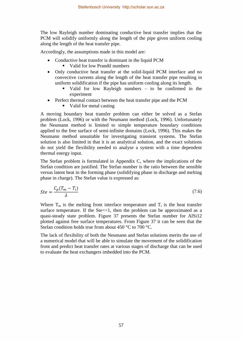
57

The low Rayleigh number dominating conductive heat transfer implies that the

PCM will solidify uniformly along the length of the pipe given uniform cooling

along the length of the heat transfer pipe.

Accordingly, the assumptions made in this model are:

Conductive heat transfer is dominant in the liquid PCM

Valid for low Prandtl numbers

Only conductive heat transfer at the solid-liquid PCM interface and no

convective currents along the length of the heat transfer pipe resulting in

uniform solidification if the pipe has uniform cooling along its length.

Valid for low Rayleigh numbers – to be confirmed in the

experiment

Perfect thermal contact between the heat transfer pipe and the PCM

Valid for metal casting

A moving boundary heat transfer problem can either be solved as a Stefan

problem (Lock, 1996) or with the Neumann method (Lock, 1996). Unfortunately

the Neumann method is limited to simple temperature boundary conditions

applied to the free surface of semi-infinite domains (Lock, 1996). This makes the

Neumann method unsuitable for investigating transient systems. The Stefan

solution is also limited in that it is an analytical solution, and the exact solutions

do not yield the flexibility needed to analyse a system with a time dependent

thermal energy input.

The Stefan problem is formulated in Appendix C, where the implications of the

Stefan condition are justified. The Stefan number is the ratio between the sensible

versus latent heat in the forming phase (solidifying phase in discharge and melting

phase in charge). The Stefan value is expressed as:

( )

(7.6)

Where Tm is the melting front interface temperature and Ti is the heat transfer

surface temperature. If the Ste<<1, then the problem can be approximated as a

quasi-steady state problem. Figure 37 presents the Stefan number for AlSi12

plotted against free surface temperatures. From Figure 37 it can be seen that the

Stefan condition holds true from about 450 °C to 700 °C.

The lack of flexibility of both the Neumann and Stefan solutions merits the use of

a numerical model that will be able to simulate the movement of the solidification

front and predict heat transfer rates at various stages of discharge that can be used

to evaluate the heat exchangers imbedded into the PCM.


58

Figure 37 - Stefan number as a function of wall temperature

7.2 Instantaneous heat transfer

Because the system can be approximated as quasi-steady at low Stefan numbers,

the instantaneous heat transfer for any charge state can be calculated using the

resistance model given that the Stefan number remains low. Thus, if the thermal

resistance of the solidified PCM is high enough, then the Stefan number will rise,

making the quasi-steady assumption invalid, and the enthalpy method for transient

analysis needs to be applied to the problem. As established in section 7.1, heat

transfer in both the liquid and the solid phases can be considered purely

conductive, simplifying the analysis considerably.

The same assumptions and conclusions that were established in section 7.1 holds

for the instantaneous heat transfer analysis. The model for both charging and

discharging is shown in Figure 38.

0

0.1

0.2

0.3

0.4

0.5

0.6

300 350 400 450 500 550 600 650 700 750

|Ste

|

Wall temperature ( C)


59

Molten PCM

Solidified PCM

Rconvective boiling/

convection

Rwall

T(rpi)

TmTbulk fluid

RPCM_S

ro

rm

ri

rpi

T(ri)

Molten PCM

Solidified PCM

ro

rm

ri

rpi

Rconvection Rwall

T(rpi)

TmTbulk fluid

RPCM_L

T(ri)

Discharging

Charging

Figure 38 - Resistance heat transfer model for charging and discharging

The resistances are calculated using equations 7.7 and 7.8. In these equations r2 is

the outer radius and r1 is the inner radius. The values for the physical properties

are taken as close to the melting point, Tm, this is possible due to the isothermal

nature of the storage system and lack of thermal properties at high temperatures

(see section 4.1)

(

)

(7.7)

(7.8)


60

The heat rates transfer is calculated using equation 7.9:

∑ (7.9)

7.3 Numerical solution to the moving boundary problem for transient

analysis

The best way to implement a numerical solution of a moving boundary problem is

the enthalpy method (Voller, et al., 1980). In the enthalpy method, the enthalpy of

each node is used to determine its temperature using enthalpy-temperature

relations. The heat transfer between nodes is calculated based on the conduction

equation (Eqn. 7.1) and the temperature of the nodes. Thus, the conservation of

energy will be applied directly rather than indirectly as in the finite difference

method (Kakac, et al., 1993).

The enthalpy method will be discussed in the form of an algorithm. Referring to

Figure 39, the entire domain (rpi<r<ro) is discretised into cylindrical shell

elements of thickness Δr. The position of the element is denoted by variable j, and

the radial position (rj) is taken in the centre of the element, with its boundaries at

rj+ Δr/2 and rj-Δr/2 respectively.

Δr

jj+1

j-1

rj

ro

rpi

Figure 39 - Discretisation of the heat transfer problem


61

Step 1 – Calculate position, volume and mass of each node

The first step is to calculate the position, volume and mass constants for each

element, which are stored in vectors r(j), V(j) and M(j) respectively. The density

of the element is taken as that of the solid AlSi12 at the melting point. The r(j),

V(j) and M(j) is calculated by equations 7.10, 7.11 and 7.12 respectively.

( ) ( ) (7.10)

( ) (( ( ) ) ( ( ) ) ) (7.11)

( ) ( ) (7.12)

Step 2 – Calculate the thermal resistance between each node

In section 7.1 it has been established that the heat transfer through the entire

problem is conductive. The steady state analytical solution for equation 7.1 can be

implemented using the resistance method (Kakac, et al., 1993). In this sense, the

heat transfer between elements is treated as quasi-steady within each time step.

The thermal resistances between the nodes (Figure 40) are stored in vector R(j),

and are calculated using equation 7.13.

j j+1

Figure 40 - Resistances between elements

( ) (

( )

( ))

(7.13)

Step 3 – Define boundary and initial conditions


62

The boundary conditions of the problem can also be represented using the

resistance model for heat transfer. Generally the heat transfer at the inner pipe at

rpi depends on the heat transfer mechanism on that boundary, and similarly on the

outside, ro, either way, the heat transfer coefficient of this boundary condition can

be calculated with the appropriate heat transfer correlation which will be

discussed along with the analysis. Convective boundary conditions are generally

represented by equation 7.14 where h represents the heat transfer coefficient.

( ) (7.14)

The initial conditions can be initialized by using the temperature vector, T(j),

which is simply the temperature of each node, or by using the internal energy

vector, E(j). The internal energy vector can be used to describe an initial condition

with a solid-liquid interface somewhere within the domain to represent a partial

charge or discharge.

If the initial temperature, Ti, is given, then:

( ) (7.15)

If Ti is above or below the melting point, the internal energy is calculated as:

( ) ( )∫ ( )

if

(7.16)

( ) ( ) (∫ ( )

∫ ( )

)

if

(7.17)

The initial enthalpy matrix H(j), is calculated by

( ) ( ) ( ) (7.18)

Step 4 – Calculate the temperature of each node

Essential to the enthalpy method is the temperature-enthalpy (T-H) relationships.

The enthalpy-temperature relationships can be derived using a DSC machine,

yielding complex T-H curves. Fortunately, eutectic materials such as AlSi12, have

a very sharp melting temperature, which results in a fairly simple, linear T-H

relations (Voller, et al., 1992). The T-H diagram for a eutectic of pure substance is

shown in Figure 41.


63

Tm T (°C)

H (

kJ/

kg)

λ

CpL

Cps

H3

H2

Figure 41 - T-H diagram for a eutectic or pure metal

The T-H relations for the eutectic system are defined in equations 7.19 through

7.24.

(7.19)

∫ ( )

(7.20)

(7.21)

( ) ( )

if

( )

(7.22)

( )

if

( )

(7.23)

( ) ( ( ) )

if

( )

(7.24)

Because the whole system is essentially on the melting point, the specific heat will

be taken as close to the melting temperature a possible and will be treated as a

constant.


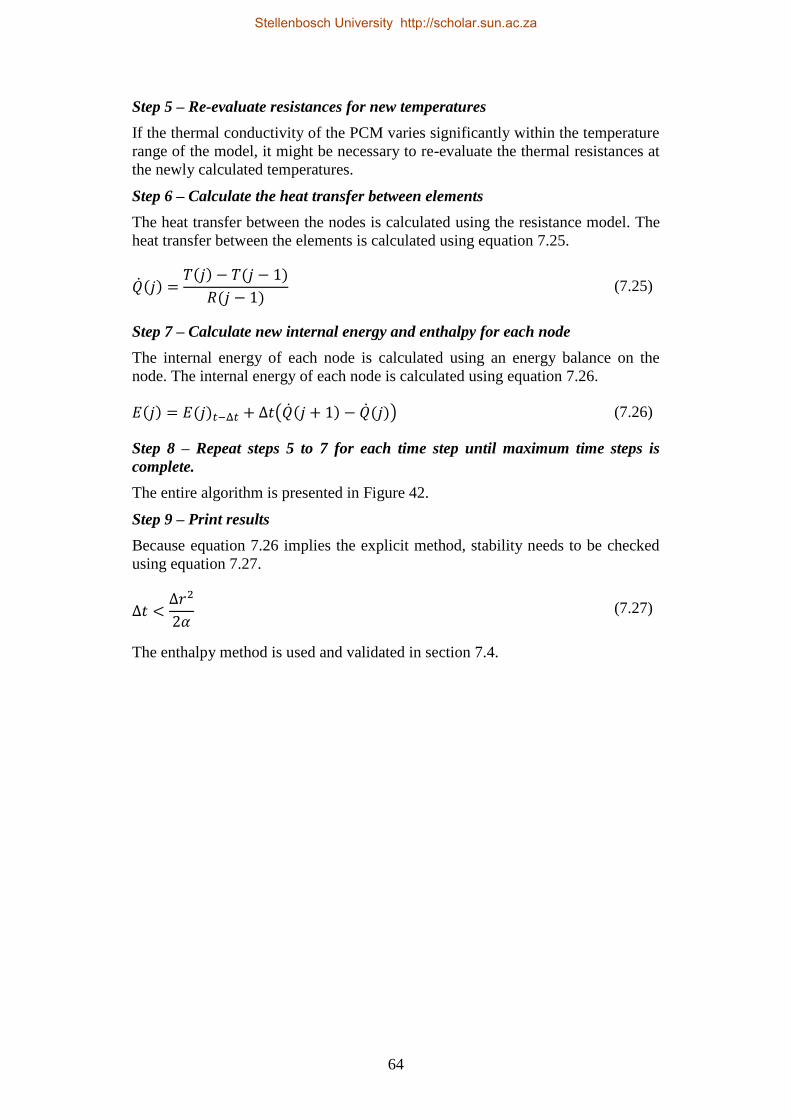
64

Step 5 – Re-evaluate resistances for new temperatures

If the thermal conductivity of the PCM varies significantly within the temperature

range of the model, it might be necessary to re-evaluate the thermal resistances at

the newly calculated temperatures.

Step 6 – Calculate the heat transfer between elements

The heat transfer between the nodes is calculated using the resistance model. The

heat transfer between the elements is calculated using equation 7.25.

( ) ( ) ( )

( ) (7.25)

Step 7 – Calculate new internal energy and enthalpy for each node

The internal energy of each node is calculated using an energy balance on the

node. The internal energy of each node is calculated using equation 7.26.

( ) ( ) ( ( ) ( )) (7.26)

Step 8 – Repeat steps 5 to 7 for each time step until maximum time steps is

complete.

The entire algorithm is presented in Figure 42.

Step 9 – Print results

Because equation 7.26 implies the explicit method, stability needs to be checked

using equation 7.27.

(7.27)

The enthalpy method is used and validated in section 7.4.


65

Problem

description:

rpi, ri, ro, L, Δr, Δt,

Ti, hpi, ho , Cp, k, ρ

Step 1 – Calculate position,

volume and mass of each node

5.7,5.8,5.9

Step 2 – Calculate the thermal

resistance between each node

5.10

Step 3 – Define boundary and

initial conditions

5.11,5.12,5.13,5.14,5.15

Step 4 – Calculate the temperature

of each node

5.16,5.17,5.18,5.19,5.20,5.21

Stable?

(5.24)

Yes

Step 5 – Re-evaluate resistances

for new temperatures

5.10

Step 6 – Calculate the heat

transfer between elements

5.22

Step 7 – Calculate new internal

energy and enthalpy for each node

5.23

t+Δt

No

Is t>tmaxPrint results Yes

E

H

T

M

R

r

V

Q

Figure 42 - Enthalpy method algorithm


66

7.4 Prototype and experimental setup

To serve as a proof of concept and to validate the analytical methods developed in

sections 7.1, 7.2 and 7.2, an experiment was devised. Liquid metals posed a

serious safety risk, and as alternative heat transfer fluid had to be used. For this

reason the storage system could not be heated up through the central heat transfer

pipe, but has to be heated with external ceramic band heaters. A single storage

element is approximated by the arrangement shown in Figure 43. It consists out of

a steel cylinder filled with AlSi12 alloy and a thick walled steel pipe running

through the centre that will act as a cooling pipe. The steel containment vessel is

heated using ceramic band heaters, and the whole assembly is wrapped in ceramic

wool for insulation. A set of five thermocouples is imbedded at various distances

from the centre of the vessel, which measure the temperature of the melt and will

enable the measurement of charge state.

Insulation

Ceramic heater bands

Outer containment wall

PCM

Heat transfer pipe

Heat transfer fluid

Thermocouples

Figure 43 - Cross section of the test section

The diameter of the outer containment shell was determined by the limitations of

the laboratory power supply. The 240V, 100A 3-phase power supply permitted

the use of three 406.4mm diameter, 330mm long ceramic band heaters, making

the outside diameter of the containment vessel 406.4mm and the length of the

vessel to 990mm excluding end caps.

Because the use of liquid metal was not permitted for safety reasons, another heat

transfer fluid had to be used. The following HTFs were considered:

Air

Water

Quenching oil


67

Preliminary heat transfer calculations revealed that the heat transfer rates using air

would be too low, and no distinct solid-liquid interface would form. On the other

hand, water also proved unfeasible because it either needs a high pressure cooling

system that resulted in an excessively expensive test rig, or the heat transfer rates

would result in two phase flow, which would complicate the measurement of heat

transfer rates. Quenching oil was considered the only viable heat transfer fluid.

A drawing of the test section is presented in Figure 44 with some of the more

important dimensions listed in Table 12. The entire test section was manufactured

from carbon steel. The internal pipe was chosen to be a BSP 1 inch S80 seamless

carbon steel pipe. It was only later discovered that molten aluminium is corrosive

to steel, which is discussed in chapter 9.

The thermocouples were placed into open ended thermocouple guide tubes to

keep them straight and in position. These were in turn held in place with a baffle

plate with location holes for the thermocouple sleeves. Unfortunately the second

thermocouple tube was accidently installed at an angle due to a mistake during

assembly, and ended up missing the guide hole in the baffle. This was only

discovered on inspection at the foundry, and could not be fixed due to logistical

reasons. The radial position of this thermocouple tube had to be re-measured

using a calliper, and is not considered accurate.

Figure 44 – Test section


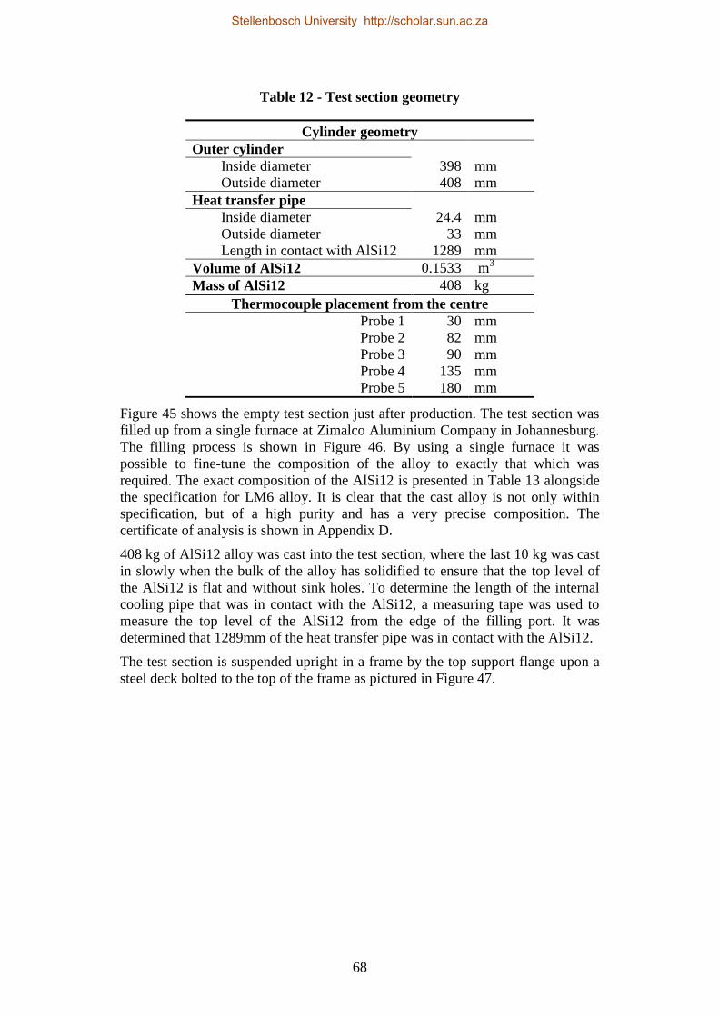
68

Table 12 - Test section geometry

Cylinder geometry

Outer cylinder

Inside diameter 398 mm

Outside diameter 408 mm

Heat transfer pipe

Inside diameter 24.4 mm

Outside diameter 33 mm

Length in contact with AlSi12 1289 mm

Volume of AlSi12 0.1533 m3

Mass of AlSi12 408 kg

Thermocouple placement from the centre

Probe 1 30 mm

Probe 2 82 mm

Probe 3 90 mm

Probe 4 135 mm

Probe 5 180 mm

Figure 45 shows the empty test section just after production. The test section was

filled up from a single furnace at Zimalco Aluminium Company in Johannesburg.

The filling process is shown in Figure 46. By using a single furnace it was

possible to fine-tune the composition of the alloy to exactly that which was

required. The exact composition of the AlSi12 is presented in Table 13 alongside

the specification for LM6 alloy. It is clear that the cast alloy is not only within

specification, but of a high purity and has a very precise composition. The

certificate of analysis is shown in Appendix D.

408 kg of AlSi12 alloy was cast into the test section, where the last 10 kg was cast

in slowly when the bulk of the alloy has solidified to ensure that the top level of

the AlSi12 is flat and without sink holes. To determine the length of the internal

cooling pipe that was in contact with the AlSi12, a measuring tape was used to

measure the top level of the AlSi12 from the edge of the filling port. It was

determined that 1289mm of the heat transfer pipe was in contact with the AlSi12.

The test section is suspended upright in a frame by the top support flange upon a

steel deck bolted to the top of the frame as pictured in Figure 47.


69

Figure 45 – Empty test section

Figure 46 - Casting of AlSi12 into test section


70

Table 13 - Chemical analysis of the cast aluminium alloy

Spec Measured

Element wt.% wt.%

Copper 0.1 max 0.01

Magnesium 0.10 max 0.01

Silicon 10.0-13.0 12.89

Iron 0.6 max 0.54

Manganese 0.5 max 0.08

Nickel 0.1 max 0.01

Zink 0.1 max 0.02

Lead 0.1 max <0.01

Tin 0.05 max <0.01

Titanium 0.2 max 0.09

Strontium na. 293 ppm

Aluminium Remainder 86.33

Figure 47 - Test section suspended in frame with heating elements and

cladding (cladding still open)


71

7.4.1 Heating elements

The heating elements around the storage unit are ceramic band heaters (pictured in

Figure 48). The size of the heaters was determined by the limitations on the

electrical supply. The properties of the heaters are as follows:

Power: 23kW max

Voltage: 3-phase 230V each

Current: 33A

Inside diameter: 406mm

Height: 330mm

Maximum operational temperature: 600°C

Figure 48 - Ceramic band heater

The band heaters is wired through an electrical panel which controls the power

delivery of the band heaters using solid state relays controlled by GEFRAN 450

PID temperature controllers. This is depicted in Figure 49. Safety features

include:

Isolator on the main distribution board

Isolator in the electrical panel

A main circuit breaker

Safety interlock toward the heater bands

300 mA earth leakage

100A ultra rapid fuses

The installed band heaters are shown in Figure 50 along with the orange electrical

panel in the background.


72

Main power

distribution

board:

3 Phase

240V

100A max

Electrical PanelBand heater 1

Top

Band heater 2

Middle

Band heater 3

Bottom

Type K thermocouple

on top band heater

Type K thermocouple

on middle band heater

Iso

lato

r

Ma

in c

ircu

it

bre

ak

er

Hea

ter

ba

nk

s

safe

ty i

nte

rlo

ck

Dis

trib

uti

on

blo

ck

Ea

rth

lea

ka

ge

30

0 m

A

Ult

ra r

ap

id f

use

s

10

0A

Cu

rren

t cl

am

ps

So

lid

sta

te r

ela

ys

Control circuit:

GEFRAN temperature controller

GEFRAN temperature cut-off

On/Off

Current display

E-Stop

L1

L2

L3

L1

L2

L3

L1

L2

L3

Figure 49 - Wiring of the three band heaters

Figure 50 – Band heaters installed around the storage vessel

7.4.2 Cooling system

The cooling of the test section was a particularly challenging design because of

the high temperature at which the AlSi12 PCM stores energy and the limitations

of regular HTFs. ISO 100 quenching oil was selected as a coolant because of its

high temperature stability and moderate heat transfer rates at high temperature

gradients. Quenching oil has the following characteristics:

High flash point

Oxidation stability

Controlled volatility

Thermal stability at high temperatures


73

The quenching oils generally come in three grades, ISO 22, ISO 32 and ISO 100.

The number indicates the oil’s viscosity index. The higher the viscosity index, the

lower the quenching oil’s cooling rate. The properties of ISO 100 quenching oil is

presented in Table 14.

Table 14 - Properties of ISO 100 quenching oil (Kopeliovich, 2013)

Density at 60°F (15.6°C) 890 kg/m³

Kinematic viscosity at 104°F (40°C) 90.2 cSt

Kinematic viscosity at 212°F (100°C) 10.6 cSt

Viscosity index 100

Flash point 267 ºC

Pour Point -9 ºC

Thermal conductivity at 104°F (40°C) 0.0106 W/m.K

Specific heat capacity at 104°F (40°C) 1950 J/(kg.K)

The oil is then cooled using water in a plate heat exchanger. The water is cooled

using a cooling tower. The cooling arrangement is illustrated in Figure 51. The oil

flow through the test section is controlled using a bypass line that is controlled

using a gate valve. All the oil piping is 1½ inch high temperature rubber hose,

piping through and close to the test section is 1 inch S40 carbon steel pipe. The

water piping is 1¼ inch Polyethylene irrigation pipe throughout.

Dump tank

Water pump:

Grundfos CM3-6

PTC

Plate HX:

Alfa Laval TL3

36 x SS304 0.4mm plates

Gate valve

F

Header tank

(Oil)

Vapour

condenser

Test section

Ball Valve

Ball Valve

Ball Valve

Solenoid valve

One-way

valve

One-way

valve

Ball Valve

Cooling

tower:

FGS7-

740-99

Heaters

Flow meter:

Laminar flow

meter

TC

FFlow meter:

Bürkert SO 55 TC

Oil Pump:

Pedrollo F 32-

200A

1" Steel pipe

1.5 " High temperature rubber tubing

1.25 " PE pipe

Legend:

TC

TC

TCP

Figure 51 – Test rig process diagram


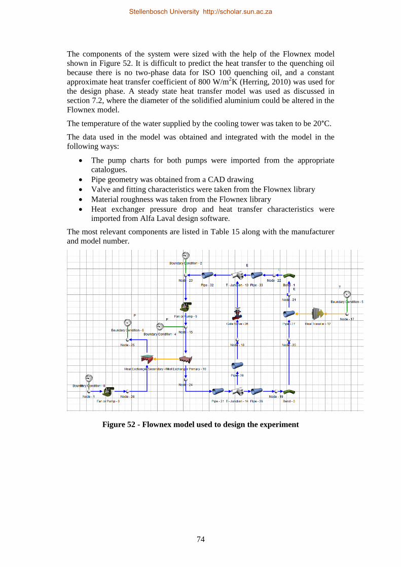
74

The components of the system were sized with the help of the Flownex model

shown in Figure 52. It is difficult to predict the heat transfer to the quenching oil

because there is no two-phase data for ISO 100 quenching oil, and a constant

approximate heat transfer coefficient of 800 W/m2K (Herring, 2010) was used for

the design phase. A steady state heat transfer model was used as discussed in

section 7.2, where the diameter of the solidified aluminium could be altered in the

Flownex model.

The temperature of the water supplied by the cooling tower was taken to be 20°C.

The data used in the model was obtained and integrated with the model in the

following ways:

The pump charts for both pumps were imported from the appropriate

catalogues.

Pipe geometry was obtained from a CAD drawing

Valve and fitting characteristics were taken from the Flownex library

Material roughness was taken from the Flownex library

Heat exchanger pressure drop and heat transfer characteristics were

imported from Alfa Laval design software.

The most relevant components are listed in Table 15 along with the manufacturer

and model number.

Figure 52 - Flownex model used to design the experiment


75

Table 15 - Cooling loop component details

Component: Manufacturer Model number

Cooling tower IWC FGS7-740-99

Water pump Grundfos CM3-6

Plate Heat Exchanger Alfa Laval TL3 -36 x SS304 0.4mm

Oil pump Pedrollo F 32-200A

The heat transfer from the test section was predicted to be about 35kW at an oil

flow rate of 0.22 kg/s.

7.4.3 Thermal insulation and losses

Insulation for the system was challenging since the band heaters had to be

operated at their upper temperature and power delivery limits, and band heater

failure meant the constant replacement of the cladding. For this reason removable

cladding bands had to be devised. The solution was to build cladding bands that

would go around each heater which could be removed individually. Because of

manufacturing limitations, the thickness of the cladding was limited to 22mm of

alkaline earth silicate wool (AES wool).

The conductive thermal resistance between the outer layer of the AlSi12 PCM and

the outside is summarised in Table 16.

Table 16 - Thermal resistance of insulating layers around the storage unit

Ther

mal

conduct

ivit

y (

W/m

K)

Thic

knes

s

(mm

)

Res

ista

nce

(°C

/W)

Sourc

e

Steel wall 22.6 5 0.00015 (Cengel, 2003)

Ceramic heating element 1.5 13 0.00572 (Technical ceramics, 2013)

AES wool 0.14 22 0.09588 (Technical Glass , 2011)

The surface temperature of the cladding was measured during the experiment

using an infrared temperature probe and was later verified using a K-type

thermocouple. The temperature was determined to be 224°C. This translates to a

thermal loss of 3462W as presented in Appendix E. This is well in agreement with

radiation and convective heat transfer predictions based on a surface temperature

of 224°C, an emissivity of 0.17 and an ambient temperature of 18°C.

The completed experimental setup is shown in Figure 53.


76

Figure 53 – The experimental setup

7.4.4 Measurements and data acquisition

The two aspects of the experiment that had to be monitored were the temperature

distribution in the melt, and the heat transfer from the test section. Data was

collected using an Agilent 34972A data logger.

All temperatures were measured using K-type thermocouples. The certification of

compliance of the thermocouples is included in Appendix D. The thermocouples

were connected to the Agilent before installation and checked at 0 and 100 °C

using ice water and boiling water. All of the thermocouples measured correctly,

passing the initial calibration. K-type thermocouples have an accuracy of

± 0.75 % (based on a 0 °C reference junction), which relates to an expected offset

of approximately 4.33 °C at 577 °C. Fortunately, the melting point of AlSi12 alloy

is fixed at 577 °C, which serves as a reference point for calibration. During the

test, the phase change is very distinct in the data set because during both the

charge and discharge the thermocouples measure a constant temperature for a fair

amount of time. By averaging the isothermal readings of each thermocouple, it

could be seen that all the thermocouples had an average offset of 4.21 °C. The

readings of the thermocouples imbedded into the molten AlSi12 were then

adapted accordingly.


77

Table 17 - Measurement errors on the test section thermocouples

Measurement Error

Probe 1 572.78 °C 4.22 °C

Probe 2 572.81 °C 4.19 °C

Probe 3 572.80 °C 4.20 °C

Probe 4 572.79 °C 4.21 °C

Probe 5 572.73 °C 4.27 °C

Average 572.78 °C 4.21 °C

To measure the heat transfer rates from the test sections, two measurement

arrangements were made. The first measured the oil flow rate and the entrance

and exit temperatures, and the other measuring the heat transfer from the oil to the

water using the water flow rate and the inlet and exit temperatures of the heat

exchanger.

Measuring oil flow rate is difficult since it has laminar flow and oil is not

conductive. For that reason a laminar flow meter had to be devised. In preliminary

design stages of the experimental setup, oil flow rates between 0.1 and 2 kg/s

were considered. The Hagen-Poiseuille equation (7.28) can be used to calculate

the flow rate of the fluid (Johnson, 1998). Is the volumetric flow rate, D is the

diameter of the pipe, L is the length and is the dynamic viscosity.

7.28

For equation 7.28 to be valid, the flow needs to be fully developed. The length of

the pipe ( ) required for laminar flow can be calculated using equation 7.29

(Johnson, 1998).

7.29

Using the properties of the thermal oil listed in Table 14 and equations 7.28 and

7.29, it was possible to design a laminar flow meter consisting of a long pipe with

two pressure taps a meter apart and 4.5m of entrance region to allow for

developed flow. The flow meter is constructed as an annulus, of which the air in

the annulus is evacuated, preventing heat transfer from the oil inside the pipe,

which could seriously affect measurements because a temperature variation in the

oil greatly affects the viscosity of the oil. The pressure is measured using an

Endress+Hauser Deltabar S PMD75 pressure transducer, which has been

calibrated using a Betz water micromanometer, of which the calibration curve is

presented in Appendix D. The details of this flow-meter are included in Appendix

D. The water flow rate is measured with a Bürkert SO 55 electromagnetic flow

meter. The calibration certificate is available in Appendix D.

All the information of the sensors and calibration information are presented in

Table 18.


78

Table 18 - Measurement devices and calibration points

Measurement Sensor Calibration range/point

Temperature probes

Test section

Probe 1 K-Type thermocouple Zero, 100 & 577 °C





Oil loop

Header tank K-Type thermocouple Zero & 100 °C

Distribution manifold K-Type thermocouple Zero & 100 °C

Test section inlet K-Type thermocouple Zero & 100 °C

Test section Outlet K-Type thermocouple Zero & 100 °C

Water loop

Heat exchanger inlet K-Type thermocouple Zero & 100 °C

Heat exchanger outlet K-Type thermocouple Zero & 100 °C

Flow meters

Oil loop

Laminar flow meter 1.12E-04 to

2.25E-03 m3/s

Water loop

Bürkert SO55 Electromagnetic flow meter 1 to 10 m/s

7.5 Experiment

The test section was first heated using the band heaters to a uniform temperature

of 630°C. During the heating of the test section, the oil is pre-heated to 40 °C by

simply passing the oil through the bypass loop with a partially closed ball valve

giving flow resistance. When the test section reached a steady and uniform

temperature of 630 °C through all the embedded thermocouples, the band heaters

were switched off and the cooling oil was re-directed through the test section and

the water cooling loop was switched on. The cooling loop was kept on until the

entire test section was cooled down to 200 °C.

The heat transfer through the cooling system could not be accurately predicted

due to the lack of two phase heat transfer data of the ISO100 oil, and therefore it

had to be measured and a correlation had to be fed back to the simulation for the

validation. The heat transfer rates from PCM to oil and from oil to water are

presented in Figure 54. The details of the heat transfer measurements are

presented in Appendix F.


79

Figure 54 - Heat transfer measurements

It was possible to do an energy balance on the storage system during latent heat

discharge by numerically integrating the heat transfer data from the beginning to

the end of latent heat discharge. The energy balance is presented in Table 19.

95.95 % of the energy that was discharged from the storage system was accounted

for by the heat transfer to the oil and calculated losses.

Table 19 - Energy balance during latent heat discharge


Mass of AlSI12 408 kg

Latent energy stored 228.48 MJ 100 %

Losses through cladding

(calculated) 16.86 MJ

7.38 %

Discharge through coolant

(measured) 202.36 MJ

88.57 %

Total heat out 219.22 MJ 95.95 %

Energy unaccounted for 9.26 MJ 4.05 %

The thermocouple readouts throughout the discharge are presented in Figure 55,

where isothermal storage is very evident, and the movement of the solidification

front is very clear where the temperature of the thermocouples drops below the

melting point of the PCM.

0

20

40

60

80

100

120

140

0 2000 4000 6000 8000

Hea

t tr

an

sfer

(k

W)

Time (s)

Heat transfer:

Oil-Water

Heat transfer:

PCM-Oil


80

Figure 55 - Thermocouple readouts throughout discharge of the storage

system

Unfortunately, this experiment could only be run once, as an unexpected

corrosion issue was uncovered during high temperature testing of steel samples

immersed into AlSi12. This posed significant safety risks. It was discovered that

molten AlSi12 is highly corrosive to most steels through mass transfer, as iron is

highly soluble into aluminium. This was unexpected, and is not readily

documented in literature. This is discussed in more detail in chapter 9.

For this reason, the data presented here is all that is available, and a replacement

test section was not possible due to budget constraints.

7.6 Numerical simulation

The entire test section was modelled as a cylinder and discretised into cylindrical

shells as discussed in section 7.2. Material properties for steel and AlSi12 was

used as presented in chapter 4 and geometry as presented in section 7.4 was used.

The inner boundary conditions for the numerical model could be expressed as:

( ) ( ) 7.30

Where PP(t) is a spline which is fitted through the measured heat transfer data

presented in Figure 54. PP(t) is a result of the built in spline function in Matlab.

450

470

490

510

530

550

570

590

610

630

0 2000 4000 6000

Tem

per

atu

re ( C

)

Time (s)

Probe 1 (°C)

Probe 2 (°C)

Probe 3 (°C)

Probe 4 (°C)

Probe 5 (°C)


81

The thermal losses towards the outside were dealt with by including the

resistances of the heating elements and cladding to the model and giving the outer

node a constant temperature as discussed in section 7.4.3.

The discretization, Δr, was chosen to be 1 mm because one of the aspects of the

moving boundary problem that must be investigated is the energy distribution

around the solidification front, and a resolution of 1mm was considered small

enough. Based on this, and the material properties listed in chapter 4, stability

criterion (equation 7.27) requires that the time step should be smaller than 9.1 ms.

The time step was made 1 ms since computational time was still within acceptable

limits.

The resulting Matlab code is presented in Appendix G.

The simulation was started with an initial temperature of 630 °C throughout. The

cooling boundary condition on the inside of the heat transfer pipe is only started

after 40 s. The temperatures of the nodes corresponding to the probes in the

experiment is plotted every 10 s, and the results is shown in Figure 56.

Figure 56 - Simulation results of the phase change problem based on the

experimental

7.7 Comparison and conclusions

The first very obvious observation that can be made from the experimental data is

that the molten part of the PCM is isothermal at the melting temperature of

AlSi12, 577 °C, confirming one of the core simplifying assumptions made. This

450

470

490

510

530

550

570

590

610

630

0 2000 4000 6000

Tem

per

atu

re ( C

)

Time (s)

SimProbe 1

(°C)

SimProbe 2

(°C)

SimProbe 3

(°C)

SimProbe 4

(°C)

SimProbe 5

(°C)


82

means that there are no convective currents in the melt, and heat transfer can be

considered as purely conductive.

By simply plotting the experimental and the simulation data over each other, as in

Figure 57, it is possible to see that the model simulates the general trends very

well apart from the transition towards the end of the discharge which is more

abrupt in the simulation than in the experiment. This can be attributed to the

constant specific heat used. The specific heat capacity of AlSi12 will have to be

determined using a differential scanning calorimeter.

Figure 57 - Experimental data and simulation data plotted over each other

for comparison

One of the key questions is if the numerical model accurately predicts the

movement of the solidification front through discharge. Figure 58 shows the

position of the thermocouples against the time when the thermocouple readout

drops below the melting point. The position of the melting point, as calculated by

the simulation, is also plotted in Figure 58 and shows good correlation with the

experimental data.

450

470

490

510

530

550

570

590

610

630

0 2000 4000 6000

Tem

per

atu

re ( C

)

Time (s)

Probe 1 (°C)

Probe 2 (°C)

Probe 3 (°C)

Probe 4 (°C)

Probe 5 (°C)

SimProbe 1 (°C)

SimProbe 2 (°C)

SimProbe 3 (°C)

SimProbe 4 (°C)

SimProbe 5 (°C)


83

Figure 58 - Comparison between the positions of solidification front as

predicted by the simulation and measured in the prototype

The assumption that quasi steady assumptions are valid is the basis for using the

resistance model for instantaneous heat transfer calculations for heat exchanger

sizing. From Figure 55 and Figure 56 it is clear that after discharge, the

temperature of the solidified mass of PCM is upheld by the discharge process and

the thermal resistance “downstream” from that location in the melt, as illustrated

in Figure 59.

Qout

T(r

m)=

Tm

T(r

pi)

T(r

pi+Δ

r)

T(r

pi+

2.Δ

r)

T(r

m-Δ

r)

T(r

m-2

.Δr)

Figure 59 - Quasi steady conduction problem

0

0.05

0.1

0.15

0.2

0.25

0 1000 2000 3000 4000 5000 6000

Posi

tion

of

soli

dif

icati

on

fro

nt

(m)

Time(s)

Position

Pedicted position


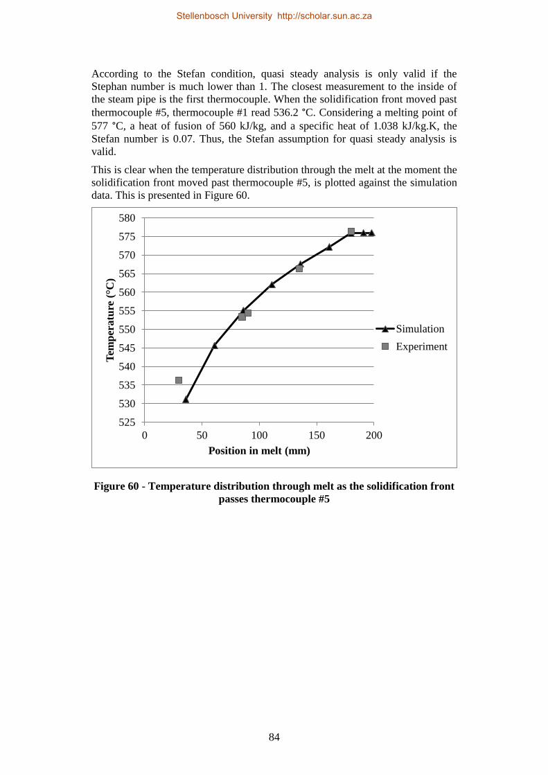
84

According to the Stefan condition, quasi steady analysis is only valid if the

Stephan number is much lower than 1. The closest measurement to the inside of

the steam pipe is the first thermocouple. When the solidification front moved past

thermocouple #5, thermocouple #1 read 536.2 °C. Considering a melting point of

577 °C, a heat of fusion of 560 kJ/kg, and a specific heat of 1.038 kJ/kg.K, the

Stefan number is 0.07. Thus, the Stefan assumption for quasi steady analysis is

valid.

This is clear when the temperature distribution through the melt at the moment the

solidification front moved past thermocouple #5, is plotted against the simulation

data. This is presented in Figure 60.

Figure 60 - Temperature distribution through melt as the solidification front

passes thermocouple #5

525

530

535

540

545

550

555

560

565

570

575

580

0 50 100 150 200

Tem

per

atu

re ( C

)

Position in melt (mm)

Simulation

Experiment


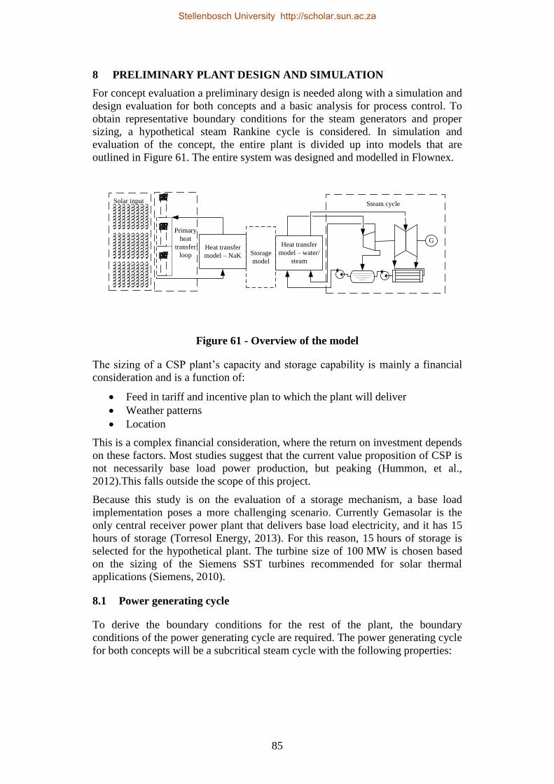
85

8 PRELIMINARY PLANT DESIGN AND SIMULATION

For concept evaluation a preliminary design is needed along with a simulation and

design evaluation for both concepts and a basic analysis for process control. To

obtain representative boundary conditions for the steam generators and proper

sizing, a hypothetical steam Rankine cycle is considered. In simulation and

evaluation of the concept, the entire plant is divided up into models that are

outlined in Figure 61. The entire system was designed and modelled in Flownex.

Storage

model

Heat transfer

model – NaK

Heat transfer

model – water/

steam

Primary

heat

transfer

loop

Solar input

G

Steam cycle

Figure 61 - Overview of the model

The sizing of a CSP plant’s capacity and storage capability is mainly a financial

consideration and is a function of:

Feed in tariff and incentive plan to which the plant will deliver

Weather patterns

Location

This is a complex financial consideration, where the return on investment depends

on these factors. Most studies suggest that the current value proposition of CSP is

not necessarily base load power production, but peaking (Hummon, et al.,

2012).This falls outside the scope of this project.

Because this study is on the evaluation of a storage mechanism, a base load

implementation poses a more challenging scenario. Currently Gemasolar is the

only central receiver power plant that delivers base load electricity, and it has 15

hours of storage (Torresol Energy, 2013). For this reason, 15 hours of storage is

selected for the hypothetical plant. The turbine size of 100 MW is chosen based

on the sizing of the Siemens SST turbines recommended for solar thermal

applications (Siemens, 2010).

8.1 Power generating cycle

To derive the boundary conditions for the rest of the plant, the boundary

conditions of the power generating cycle are required. The power generating cycle

for both concepts will be a subcritical steam cycle with the following properties:


86





and

Air-cooled condenser (ACC) with a condenser pressure of 0.15 bar.

A process diagram of the Rankine cycle is shown in Figure 62 and a T-s diagram

of the power cycle is shown in Figure 63. The numerical annotation is consistent

throughout these two figures.

LP

Turbine

G

HP

Turbine

Open

FW heater

LP FW

Pump

6

HP FW

Pump

10

7

Re-heater

Super heater

Boiler

3

1

8

9

2

Air cooled

condenser

4

5

Tamb=30°C

Figure 62 - Power generation cycle


87

100

200

300

400

500

1 2 3 4 5 6 7

3

1

45

7

6

2

8

9

Entropy (kJ/kg.K)

Tem

per

ature

(°C

)

Figure 63 - T-s diagram for the power cycle

Flownex SE was used to provide a complete simulation environment where heat

transfer, fluid mechanics and thermodynamics could be simulated simultaneously

in both steady state and in transient state. To provide initial design parameters for

the Flownex model, the power cycle first had to be evaluated by hand. The

detailed hand calculation of the power cycle is presented in Appendix H. The

energy balance of the power cycle is presented in Table 20. The overall thermal

efficiency of the cycle is 38 %, which is within the expected range for such a

simplified steam cycle. It must be noted that the thermal efficiencies of the

components are not based on the performance of actual hardware and taken to be

approximate values for these components as stated in literature (Cengel, et al.,

2002) (Karassik, et al., 1985) (Johnson, 1998).

The steam generator is divided into three distinct sections:

Boiler

Super-heater

Re-heater

These will be considered separately throughout. The boundary values yielded by

hand calculations are shown in Table 21.


88

Table 20 - Energy balance of a hypothetical power cycle

Mass flow

(kg/s) (MW) Efficiency

Thermal input

Boiler 93.99 151.7 Super-heater 93.99 74.83 Re-heater 68.01 34.01 Total 260.54

Pump electrical input

Pump 1 68.01 0.24 0.85

Pump 2 93.99 1.48 0.85

Total 1.72

Heat removed by the condenser

Condenser 68.01 156.99

Turbine output

Turbine 1 93.99 36.39 0.87

Turbine 2 68.01 68.87 0.87

105.26

Generator 100 95

Overall thermal efficiency 0.38


generator

Mass

flow

(kg/s)

Enthalpy

change

(kJ/kg) (MW) Tin(°C) Tout(°C) P(bar)

Boiler 93.99 1613.98 151.70 236.85 336.67 140

Super-heater 93.99 796.11 74.83 336.67 540 140

Re-heater 68.01 500.01 34.01 321.17 540 30

The Flownex model is built up using the hand calculations as a starting point. The

Flownex model is based on exactly the same theory and assumptions as the hand

calculations and thus the energy balance and the boundary conditions are the same

as in Table 20 & Table 21. The details of the Flownex model are shown in

Appendix I. The basic Flownex model used in the Rankine cycle is presented in

Figure 64.


89

Figure 64 - Flownex model of the Rankine Cycle

The model shown in Figure 64 is used as a basis throughout the rest of this text

because most of the design work was done with the aid of the “Flownex

designer” tool. The designer tool uses the Newton-Raphson solution algorithm to

solve a set of non-linear equations that relates to the dependent and independent

variables of the flow network. The relation between the independent variables

(such as orifice diameter or turbine efficiency) is set by the user, and the

dependent variables (such as mass flow rate, pressure drop and flow velocity) in

the designer interface. By setting goals for the dependent variables and a domain

for the independent variables with initial guess values, the designer will find a

solution that best suits the scenario.

8.2 Primary heat transfer loop

The solar thermal input of the power generating system is dependent on a number

of factors mostly related to the time dependent input of the sun. The solar resource

is available in a sinusoidal fashion, and has to be concentrated by the collector

field and absorbed by the receiver. The collector field has its own characteristic

behaviour which is highly dependent in the exact nature of the heliostats, heliostat

field layout, tower height and weather conditions. Furthermore, the exact design

of the receiver also has a large effect on the efficiency and characteristics of the

system as a whole. Because the focus of this project is not the collector or the

receiver itself, some simplifying assumptions are necessary. The aim is to obtain

peak design parameters for the receiver loop that are representative of what may

be encountered in a real central receiver plant.

To design the heat exchangers for the primary cooling loop the peak design heat

transfer requirements are necessary. The primary heat transfer loop of the DSG

concept is illustrated in Figure 65. The factors influencing both the peak heat

transfer requirements and the nature of the heat exchange elements are discussed

in the subsequent subsections.


90

Super heater

Boiler

Re-heater

Receivers

Figure 65 - Heat exchanger configuration for the DSG concept

8.2.1 Primary loop heat transfer requirements

The time dependent thermal input of the solar collector and receiver system must

be considered to calculate the peak heat transfer requirements of the primary heat

transfer loop of the plant. The thermal input from the collector field to the receiver

is the product of the direct normal irradiation (DNI) and the collector field

efficiency. The collector field’s efficiency depends on the design of the field and

is also time dependent. The specific design of the field is outside of the scope of

this study, and the field efficiency is taken to be constant throughout the day.

Consequently the time dependent profile of the thermal input can therefore be

taken as the normalized DNI (Battleson, 1981) (Steine, et al., 1986) (Meduri, et

al., 2013). To determine the location of the plant, a map of the South African

annual DNI is presented in Figure 66, p.92.

The annual DNI is the annual sum of the DNI on that location and is measured in

kWh/m2. The map in Figure 66 indicates the best places for such a power plant.

The higher the DNI, the more power is produced per square meter of the collector,

which brings down the LCOE. In this project, Upington (28°24′0″S, 21°16′0″E) is

chosen as the location of the hypothetical plant due to high DNI , good supply of

water, and the existing grid connection in the area (Fluri, 2009).

The DNI for a given location can be calculated accurately, and the Bird Clear Sky

Model (Bird, et al., 1981) is taken to be the industry standard model to calculate

the clear sky DNI at any given time assuming clear skies. The DNI values in

Upington for four seasons are shown in Figure 67, p.92.


91

Figure 66 - Annual DNI for South Africa (Geosun)

Figure 67 - Clear sky DNI for Upington

0

200

400

600

800

1000

1200

00:0

0:0

0

03:0

0:0

0

06:0

0:0

0

09:0

0:0

0

12:0

0:0

0

15:0

0:0

0

18:0

0:0

0

21:0

0:0

0

00

:00

:00

DN

I (W

/m2)

Time(hh:mm:ss)

Summer

Winter

Spring/Autumn


92

The primary heat transfer loop transports thermal energy from the receiver to the

HSU and the power block. Because solar energy is time dependent, the receiver

will have to have a peak working point where the receiver must absorb all the

incoming radiation from the collector field. The normalized DNI dictates the time

dependent “shape” of this thermal input since the assumption is based on the

collector field having a constant optical efficiency throughout the day. Figure 68

presents the normalized DNI in Upington for summer, winter and spring.

Figure 68 - Normalized DNI for the summer solstice, winter solstice and the

southward equinox (spring) for Upington

Designing the field for the winter will result in significant defocussing in summer

and designing for the summer will result in excessive co-firing in the winter. A

financial evaluation is required to find an optimum collector field size. To

simplify the analysis, the time dependent input for the southward Equinox for

2013 (Spring – 22nd

September) will be used as a basis for the time dependent

thermal input,( ( )). The primary heat transfer loop is to be sized to achieve full

charge (15h) on a day with no clouds on the southward equinox. It must be noted

that proper sizing of the thermal energy storage system is a complex study, and

falls out of the scope of this project, and this crude assumption will have to

suffice.

The receiver was sized using an energy balance of the storage system for one day

illustrated in Figure 69. The heat transfer requirements to the steam generator

( ) is calculated in section 8.1 and is presented in Table 21. This yields a time

dependent problem since the heat transfer from the primary cooling loop has a

certain profile.

0

0.2

0.4

0.6

0.8

1

00:0

0:0

0

03

:00

:00

06:0

0:0

0

09:0

0:0

0

12

:00

:00

15:0

0:0

0

18:0

0:0

0

21

:00

:00

00:0

0:0

0

Norm

ali

zed

DN

I

Time(hh:mm:ss)

Summer

Winter

Spring/Autumn


93

= 260.54 MW

Storage

Qin(t) Qout

Qstore

SG

Figure 69 - Energy balance to storage

The heat transfer to the storage system is calculated by multiplying the normalized

DNI by the peak heat transfer rate:

( ) ( ) (8.1)

Where:

(8.2)

SM is the solar multiple. The energy delivered to storage is calculated by:

∫ ( )

(8.3)

and the energy delivered to the steam generators:

∫ ( )

(8.4)

The size of the storage can be calculated by

(8.5)

The energy balance yields:

(8.6)

Substituting equation 8.2 into equation 8.1 and substituting that into equation 8.6

and substituting equations 8.4 and 8.5 into equation 8.6:


94

∫ ( )

∫ ( )

(8.7)

Since and is known, the solar multiple, SM, can be calculated. The

function ( ) was given by the Bird clear sky model and the integration was

performed for a period of one day (since full charge is needed after one day). The

resulting solar multiple is 2.73, which results in a peak heat transfer rate of

711.80 MW for the primary heat transfer loop. The time dependent energy

balance is presented in Figure 70.

Figure 70 - Power to and from storage

It is possible to calculate the peak heat transfer rates to each storage section for the

DSG concept by taking the ratios of the heat transfer requirements between the

boiler, super- and re-heater (Table 21) and applying them to the peak heat transfer

rate of the primary cooling loop. This is presented in Table 22.

Table 22 - Heat transfer requirements for the primary heat transfer loop

(MW) (MW)

Boiler 151.7 414.44

Super-heater 74.83 204.44

Re-heater 34.01 92.92

Total 260.54 711.80


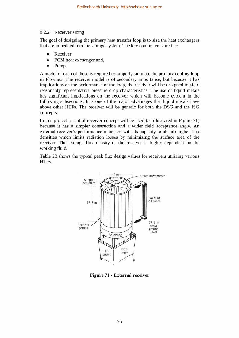
95

8.2.2 Receiver sizing

The goal of designing the primary heat transfer loop is to size the heat exchangers

that are imbedded into the storage system. The key components are the:

Receiver

PCM heat exchanger and,

Pump

A model of each of these is required to properly simulate the primary cooling loop

in Flownex. The receiver model is of secondary importance, but because it has

implications on the performance of the loop, the receiver will be designed to yield

reasonably representative pressure drop characteristics. The use of liquid metals

has significant implications on the receiver which will become evident in the

following subsections. It is one of the major advantages that liquid metals have

above other HTFs. The receiver will be generic for both the DSG and the ISG

concepts.

In this project a central receiver concept will be used (as illustrated in Figure 71)

because it has a simpler construction and a wider field acceptance angle. An

external receiver’s performance increases with its capacity to absorb higher flux

densities which limits radiation losses by minimizing the surface area of the

receiver. The average flux density of the receiver is highly dependent on the

working fluid.

Table 23 shows the typical peak flux design values for receivers utilizing various

HTFs.

Figure 71 - External receiver


96

Table 23 – Typical receiver peak flux design values (Battleson, 1981)

Heat transfer Fluid

Designed

peak flux

(MW/m2)

Liquid sodium 1.5

Molten nitrate salt 0.7

Liquid water 0.7

Steam vapour 0.5

Air 0.22

It is clear that a receiver using liquid sodium would be less than half the size of a

receiver using molten nitrate salt or water, reducing thermal losses by half.

Liquid sodium receivers have been tested by both SANDIA labs, and by PSA.

The receiver tested at PSA could achieve a peak flux density of 2.5 MW/m2 with a

receiver efficiency of 90 %. (Schiel, 1988).

The construction of a liquid metal receiver is relatively simple, and is similar to

water and molten salt receivers. The receiver tested at the PSA was constructed by

an Italian company, Franco Tosi. It consisted of a plate of parallel pipes, with two

headers. Five panels were constructed for the single receiver. A schematic of the

receiver is shown in Figure 72. The panels were covered in Pyromark™ paint.

Figure 72 - Liquid sodium receiver tested at PSA (Schiel, 1988)

Because the dominating heat transfer characteristic of sodium is its high thermal

conductivity, it is possible to generalize the attributes of a liquid sodium receiver

to other liquid metals, and it is theoretically possible to constrict similar receivers

using other liquid metals like NaK and Lead Bismuth alloy.


97

The use of liquid metals as HTFs enables the construction of compact,

lightweight, more efficient receivers, with simple design geometry that can

operate at higher temperatures than possible with other HTFs.

For this project, a peak heat flux density of 2.5 MW/m2 (Schiel, 1988) in an

external receiver will be assumed with a maximum operational temperature of

800 °C due to the material limits of Inconel X750 (Special Metals Corperation,

2013). It is possible to determine the most suitable heat transfer exit temperature

based on the combined thermal efficiency of the power block, storage and

receiver.

As discussed in section 8.2.1, the receiver should be able to deal with 711.80 MW

of heat flux. The receiver will be divided into three equally sized 237.2 MW

receivers due to field limitations.

Because there are no commercial liquid metal receivers, no pressure drop and

flow data available on the experimental receivers that was tested by PSA and

SANDIA (Schiel, 1988), some crude assumptions will have to be made to size a

receiver.

The heat transfer fluid pressure and temperature of the receiver will be found in an

iterative manner using Flownex, and the wall thickness of the pipes adapted

accordingly. Considering three separate receivers with uniform flux distribution (a

valid assumption at noon with a properly designed field) each with a flux density

of 2.5 MW/m2, yields a surface area of 94.91m

2 for each of them. The surface area

is calculated on the outer diameter of the receiver and not the surface of the

physical pipes. A roughly square target is preferred for the aiming of the

heliostats, and using a rounded up surface area of 95m2 a diameter of 5.5m and a

height of 5.5m are calculated.

The receiver is constructed of parallel tubes made of Inconel 800 coated with

Pyromark™ paint. To evaluate the most suitable tube size, a mass flow rate of

7550 kg/s and an inlet temperature of 590 °C is used. The exit temperature is

calculated as 692.38 °C using the properties presented in section 4.2. The mass

flow rate of the NaK is relatively high due to the low Cp value of NaK, and

therefore a low pressure drop is important to keep pumping power to a minimum.

Because Inconel tube is made according to specification (Special Metals

Corperation, 2013), and the pressure and temperature for the receiver are not

known at this stage of the analysis, the tube wall thicknesses is taken as that of

ANSI B36.19 steel tube.

The receiver is simply an array of tubes running along the circumference of the

receiver with their outer wall tangential to the outer diameter of the receiver. The

pressure drop was calculated for the receiver with the pre-selected conditions for

each standard B36.19 tube diameter from 1/8 inch to 2 inch. Pressure drop in

liquid metals flowing in tubes is calculated in the same manner as for water and

other liquids (Liquid metal engineering center, 1972), and the Darcy-Weisbach

(Darcy, 1857) (Weisbach, 1845) equation is used with a surface roughness of


98

60μm, which is typical for seamless steel tubes (Special Metals Corperation,

2013). The results are presented in Table 24 and are plotted in Figure 73.

Table 24 - Pressure drop for various heat transfer tube diameters for the

receiver

B36.19

designation

Outside

diameter

(mm)

Wall

thickness

(s40)

Inside

diameter

(mm)

Pressure

drop

(kPa)

Pipes per

receiver

Number

of pipes

(total)

1/8" 10.3 1.73 5.68 90656.73 1673 5019

1/4" 13.71 2.24 9.23 12130.23 1256 3768

3/8" 17.14 2.31 12.52 3767.88 1004 3012

1/2" 21.34 2.77 15.8 1706.59 806 2418

3/4" 26.67 2.87 20.93 605.80 644 1932

1" 33.4 3.38 26.64 266.81 514 1542

1 1/4 " 42.16 3.56 35.04 101.23 406 1218

1 1/2" 48.26 3.68 40.8 59.57 355 1065

2" 60.32 3.91 52.5 25.01 283 849

Smaller tube diameters are favourable for heat transfer because thinner walls can

be used, a significant factor if the low thermal conductivity of Inconel is

considered (Special Metals Corperation, 2013). By plotting the pressure drop

versus tube diameter (Figure 73) it can be seen that 1-inch (33mm outside

diameter) tube yields an acceptable 266.81 kPa pressure drop at peak flow rates.

Figure 73 - Pressure drop over receiver versus outer diameter for various

B36.19 tubes

0.00

200.00

400.00

600.00

800.00

1000.00

1200.00

1400.00

1600.00

1800.00

20 30 40 50 60 70

Pre

ssu

re d

rop

(k

Pa)

Outside diameter -S40 (mm)


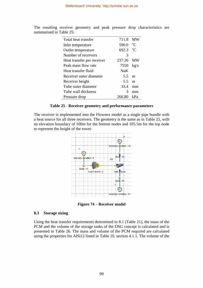
99

The resulting receiver geometry and peak pressure drop characteristics are

summarised in Table 25:

Total heat transfer 711.8 MW

Inlet temperature 590.0 °C

Outlet temperature 692.3 °C

Number of receivers 3

Heat transfer per receiver 237.26 MW

Peak mass flow rate 7550 kg/s

Heat transfer fluid NaK

Receiver outer diameter 5.5 m

Receiver height 5.5 m

Tube outer diameter 33.4 mm

Tube wall thickness 3 mm

Pressure drop 266.80 kPa

Table 25 - Receiver geometry and performance parameters

The receiver is implemented into the Flownex model as a single pipe bundle with

a heat source for all three receivers. The geometry is the same as in Table 25, with

an elevation boundary of 100m for the bottom nodes and 105.5m for the top node

to represent the height of the tower.

Figure 74 – Receiver model

8.3 Storage sizing

Using the heat transfer requirements determined in 8.1 (Table 21), the mass of the

PCM and the volume of the storage tanks of the DSG concept is calculated and is

presented in Table 26. The mass and volume of the PCM required are calculated

using the properties for AlSi12 listed in Table 10, section 4.1.1. The volume of the


100

heat exchangers (section 8.4) and the dead volume (chapter 7) are added to the

total volume of the tank. The dimensions of these tanks are presented in Table 27.

Table 26 - Mass and volume required for 15h of thermal energy storage

(MW)

Energy

storage

(GJ)

Mass of

PCM

(Ton)

Volume

(m3)

Total

volume of

imbedded

heat

exchangers

(m3)

Dead

volume

Total

volume

of the

tank (m3)

Boiler 151.7 8191.80 14628.21 5714 72.13 561.25 6347.38

Super-

heater 74.83 4040.82

7215.75 2819 47.66 278.07

3144.73

Re-heater 34.01 1836.54 3279.54 1281 32.42 127.40 1440.82

Total 260.54 14069.16 25123.50 9814 152.21 966.72 10932.93

Table 27 - Size of the storage tanks

Boiler

Super-

heater Re-heater

Tank diameter 36.61 m 28.23 m 18.06 m

Tank height 6 m 5 m 5 m

The height of the tanks is determined by the length of the heat exchangers, which

is determined by the heat transfer requirements of both the NaK and the

water/steam generators.

The ISG concept has one tank with one heat exchanger embedded into the PCM.

The details of the storage tank are shown in Table 28.

Table 28 - ISG storage sizing

(MW) 260.54 MW

Energy storage (MJ) 14069.16 GJ

Mass 25123.50 Ton

Volume 9813.87 m3

Volume of heat exchanger 69.39 m3

Total volume of the tank with dead volume included 10842 m3

Height of tank 6 m

Diameter of tank 47.97 m


101

8.4 Heat exchanger sizing and modelling

Seven heat exchangers had to be sized:

PCM – Water/steam heat exchangers for the DSG concept

Boiler

Super-heater

Re-heater

NaK – PCM heat exchangers for the DSG concept

Boiler

Super-heater

Re-heater

NaK – PCM heat exchangers for the ISG concept

To size the heat exchangers the extreme heat transfer parameters must be designed

for and provision has to be made for process control for all intermediate

conditions. As discussed in chapter 7, the solidified PCM around the heat transfer

pipe adds thermal resistance to the heat exchanger and changes the heat transfer

characteristics of the heat transfer surfaces. In other words, the heat exchangers

have to be designed for both fully charged and nearly fully discharged conditions

at nominal heat transfer rates.

As mentioned in chapter 7, the NaK and steam/water heat exchangers will be

considered separately for simplification of the analysis, and this is merited by the

fact that the critical design points of the steam generator in the DSG concept is

during discharge only.

The basic variables of the heat exchangers in the steam generator sections include

the length of the heat-transfer pipes; the number of tubes; and the tube size. A

discretised model of these heat transfer surfaces is implemented in Flownex; and

the model is then used to obtain the sizing of the heat transfer surfaces.

All of the heat exchanger sizing and heat transfer analysis was done in Flownex.

The heat exchangers were first separately designed using the boundary conditions

determined in sections 8.1 and 8.2 and was implemented as illustrated in Figure

75 below. The separate models were then incorporated into the larger Flownex

model to evaluate the overall system performance parameters and to evaluate the

effect on various operational conditions.

The instantaneous heat transfer model discussed in section 7.2 is used for the heat

exchanger sizing. This is implemented into Flownex using a heat transfer element

as shown in Figure 75. The heat transfer element can be set up to include

radiation, conduction and convection of various geometries. The pipe element can

be set up to determine the pipe geometry, number of parallel pipes, and problem

discretization. Discretization is set up by setting the number of serial increments

the pipe is divided into. The heat transfer model is also automatically discretized

along the length of the pipe, and the same manner of discretization is possible

with the conduction heat transfer models. The level of discretization can be set

using a sensitivity analysis tool, which is used to automatically determine the


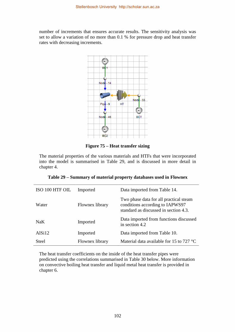
102

number of increments that ensures accurate results. The sensitivity analysis was

set to allow a variation of no more than 0.1 % for pressure drop and heat transfer

rates with decreasing increments.

Figure 75 – Heat transfer sizing

The material properties of the various materials and HTFs that were incorporated

into the model is summarised in Table 29, and is discussed in more detail in

chapter 4.

Table 29 – Summary of material property databases used in Flownex

ISO 100 HTF OIL Imported Data imported from Table 14.

Water Flownex library

Two phase data for all practical steam

conditions according to IAPWS97

standard as discussed in section 4.3.

NaK Imported Data imported from functions discussed

in section 4.2

AlSi12 Imported Data imported from Table 10.

Steel Flownex library Material data available for 15 to 727 °C

The heat transfer coefficients on the inside of the heat transfer pipes were

predicted using the correlations summarised in Table 30 below. More information

on convective boiling heat transfer and liquid metal heat transfer is provided in

chapter 6.


103

Table 30 – Summary of correlations used in the Flownex simulations

Single phase heat transfer for water Gnielinski (Gnielinski, 1975)

Two phase heat transfer for water Steiner and Taborek (Steiner, et al.,

1992)

Pressure drop for single phase water Darcey-Weisbach (Darcy, 1857)

(Weisbach, 1845)

Pressure drop for two phase water Lockheart -

Martenelli

(Lockheart, et al.,

1949)

Heat transfer correlation for single

phase liquid metal Seban-Shimazaki

(Liquid metal

engineering

center, 1972)

Pressure drop for single phase liquid

metal flow Darcey-Weisbach

(Darcy, 1857)

(Weisbach, 1845)

The onset of nucleate boiling, saturated boiling and Leidenfrost points are

calculated automatically in Flownex (Flownex, 2011). The Leidenfrost point is

where the liquid water separates from the heat transfer surface and forms a

sustained vapour layer. In transition boiling, a linear extrapolation between the

critical heat flux and the minimum heat flux points is used (Flownex, 2011); and

for film boiling the Zuber correlation is used (Flownex, 2011).

On the PCM side of the heat transfer surfaces (the heat transfer pipes are

embedded into the PCM), there is a moving boundary problem. As the storage

system discharges, solidified PCM builds up around the heat transfer pipes,

causing a variation in the heat transfer characteristics of the heat exchange

surfaces.

The maximum diameter of the PCM build-up (do), is calculated by dividing the

volume of the PCM by the number of heat transfer pipes of one of the heat

exchangers imbedded in it, and then calculating the distance between the sides of

a hexagon of that volume. The critical design points for the heat exchanger are full

charge, when the heat exchanger has no solidified PCM around it; and near full

discharge where the solidification front meets the maximum diameter. In the

Flownex model, the solidification front was calculated using an energy balance

for transient simulations. A spread sheet was built into the Flownex model which

automatically calculated the dependent variables such as do, storage volume and

overall tank geometry based on heat exchanger geometry and storage

requirements.

The heat exchangers were designed with the Flownex design tool. The Flownex

design tool was set to yield the required heat transfer rates at near discharge

conditions. Pressure drop was taken into account, but the pipe diameter and

lengths were fixed for simplification. The diameters of all the steam pipes were

set to a B36.19 1 inch S80 steam pipe for all the heat transfer surfaces. Steel was

used for the heat water/steam heat exchangers, and stainless steel 306 was used

for the NaK heat exchangers. The lengths of the pipes were found through a


104

number of design iterations that would satisfy both the NaK and the steam/water

heat exchangers.

8.4.1 Steam/water Heat exchangers for the DSG concept

For the plant to operate at steady conditions, the effect of the moving boundary

needs to be counteracted. There is nothing that can be explicitly controlled about

the energy source to the heat transfer surfaces (as in a gas-fired boiler), and the

only feasible method of control is to manage the flow in the heat exchangers.

Flow boiling is a function of both convective boiling heat transfer and nucleate

boiling heat transfer (Steiner, et al., 1992). To have a controllable steam generator,

the convective-boiling heat transfer should be the controlling heat transfer

mechanism in the heat exchanger, especially close to complete discharge.

For the boiler, the objective is to deliver saturated dry steam at the feedwater flow

rate. Dry out of the boiler tubes is prevented by keeping the vapour fraction

sufficiently low in the boiler itself, and this means that the flow rate though the

boiler should be multiple times that of the feedwater. The process layout is shown

in Figure 76 and the Flownex model of the boiler is presented in Figure 77. The

model was used to determine the operational limits of the boiler circuit. The boiler

circulation rate is adjusted to meet the heat transfer requirements throughout

discharge. The upper and lower boiler circulation rate is presented in Table 32

along with heat transfer coefficients. The heat exchanger geometry for the boiler

is presented in Table 31.

Boiler

Steam

drum

Pump

Variable

flow rate

NaK to receiver

NaK from receiver

To Superheater

Figure 76 - Boiler arrangement


105

Figure 77 – Boiler model

Because the super-heater and re-heater operate as single phase systems, it is

possible to bypass some of the steam past the re-heater or super-heater, and mix it

with the superheated steam that went through the heat transfer pipes. This

arrangement is illustrated in and Figure 78 and the generic Flownex model for

both are presented in Figure 79. The heat exchangers for both the super-heater and

re-heater were designed to deliver superheated steam with all of the steam running

through the heat exchanger at the end of its charge and with steam diverted past

the heat exchangers at higher charge states. The bypass rates and the average heat

transfer coefficients are presented in Table 32. The heat exchanger geometry is

presented in Table 31.

Superheated steam to

turbine

NaK to

receiver

NaK from

receiver

Steam from boiler/HP

turbineMixing

drum

Re-heater/

super-heater

Figure 78 - Re-heater and super-heater arrangement


106

Figure 79 – Re-heater and super-heater model

Table 31 – Steam water heat exchanger geometry

Boiler Super-heater Re-heater

Number of steam pipes 300 820 1000

Diameter of steam pipes 33.40 mm 33.40 mm 33.40 mm

Wall thickness 4.55 mm 4.55 mm 4.55 mm

Passes Single Double Double

Length 6 m 5 m 5 m

Material MS MS MS

Volume of heat exchanger 6.30 m3 14.36 m

3 17.52 m

3

Maximum PCM diameter, do 2.01 m 0.66 m 0.38 m


107

Table 32 – Steam/water heat exchanger control strategy

Full charge Low charge

Boiler

Boiler circulation rate 209.00 kg/s 213.00 kg/s

Heat transfer 151.70 MW 151.70 MW

Average convective boiling heat

transfer coefficient 6069.9 W/m

2.K 6937.49 W/m

2.K

dm 0 m 2.01 m

Super-

heater

Super-heater bypass 2.77 % 0.33 %


Average convective heat


2.K 2557.21 W/m

2.K

dm 0 m 0.66 m

Re-heater

Re-heater bypass 9.01 % 8.22 %


Average convective heat


2.K 1246.03 W/m

2.K

dm 0 m 0.38 m

8.4.2 NaK heat exchangers for the DSG concept

The isothermal nature of the storage unit decouples the heat transfer of the steam

heat exchangers from that of the NaK heat exchangers; allowing the NaK loop to

be considered separately. In the DSG concept, the NaK heat exchangers have to

be designed to transfer all the thermal energy from the receivers to the storage

units during peak conditions. In the DSG concept the NaK heat exchangers are

divided between the boiler, super-heater and re-heater. The NaK flow is diverted

according to the ratios of the energy removed by the steam generator. The heat

transfer requirements for each heat exchanger are shown in Table 33.

Table 33 – NaK flow distribution

(MW) Ratio

(MW)

Inlet

temperature

(°C)

NaK mass

flow

(kg/s)

NaK

volume

flow (m3/s)

Boiler 151.70 0.58 414.43 692.3 4396.00 6.04

Super-

heater 74.83 0.29 204.43 692.3 2168.44 2.98

Re-

heater 34.01 0.13 92.91 692.3 985.55 1.35


108

These requirements were used as boundary conditions in Flownex to size the heat

exchanger. The critical design points are at maximum heat transfer rates, and

close to full charge, where the layer of molten PCM is the largest. This design

point was used in Flownex to size the heat exchangers. Again, for simplification,

the heat exchanger pipes were kept to 1 inch S80, but are made of stainless steel

306. The length of the pipes is fixed to be the same as the length of the

water/steam heat exchanger pipes.

Table 34 – NaK heat exchanger geometry for the DSG concept

Boiler

Super-

heater Re-heater

Number of steam pipes 3130 1900 850

Diameter of steam pipes 33.40 mm 33.40 mm 33.40 mm

Wall thickness 4.55 mm 4.55 mm 4.55 mm

Passes Single Single Single

Length 6 m 5 m 5 m

Material SS SS SS

Pressure drop during peak flow 40.32 kPa 22.36 kPa 22.97 kPa

Maximum efficiency 0.93 0.93 0.93

Volume of heat exchanger 65.81 m3 33.29 m

3 14.89 m

3

8.4.3 Heat exchangers for the ISG concept

The ISG has one NaK-PCM heat exchanger for both charging and discharging as

illustrated in Figure 80. During charging all the NaK is directed through the

receivers and then through the storage bank. From the storage bank the NaK will

flow to the steam generator system. A liquid metal steam generator system is an

extremely specialized piece of equipment and will not be dealt with in detail, as it

falls outside the scope of this project. The steam generator was simulated as a pipe

with a pre-set heat loss equal to the heat transfer requirements for the power cycle.

As shown in Figure 70 (section 8.2), the peak heat transfer rate from the receiver

is 711.8 MW, and the heat transfer to the steam cycle is constant at 260.54 MW.

Therefore, during charging the heat exchanger has to transfer 451.26 MW to the

PCM, and during discharge it has to transfer 260.54 MW from the PCM to the

NAK HTF.

The same receiver model used in the DSG concept was implemented in the ISG

loop, and the peak receiver outlet temperature was kept at 693.45 °C for

consistency. The heat exchanger length was chosen as 6m and again S80 1 inch

stainless steel pipe was chosen for the heat exchanger.

The Flownex model in Figure 81 was used to size the heat exchanger and

determine operational parameters.


109

Figure 80 – ISG heat transfer and storage

Figure 81 - Primary cooling loop for the ISG concept

The critical design point for the heat exchanger is charging conditions at near full

charge and these conditions were used to get the design geometry presented in

Table 35. The control strategies that would have to employed to control the

primary cooling loop in the ISG system would be very complicated, and the

design parameters of the steam generator must be known. The Flownex model can

be used for these studies.


110

Table 35 – NaK heat exchanger geometry, storage tank dimensions and

operational parameters

Heat exchanger geometry

Number of steam pipes 3300

Diameter of steam pipes 33.40 mm

Wall thickness 4.55 mm

Passes 1

Length 6 m

Material SS

Volume 112.70 m3

Tank geometry

Height 6 m

Diameter 47.97 m

Volume 112.70 m3

do 0.8 m

Operational parameters: Charging (Full charge)

dm 0.8 m

NaK mass flow rate through HX 7550 kg/s

Pressure drop during peak conditions 107.51 kPa

Bypass: 0 %

Heat transfer coefficient 1405.20 kW/m2K


111

8.5 Overall model

From section 8.1 to section 8.4 all major components of the power generating

cycle were designed and simulated for both the DSG and ISG concepts in separate

design cases using the boundary conditions of the power cycle determined in

section 8.1. The separate components could then be integrated into one single

model to demonstrate the ability of Flownex to simulate an entire CSP plant.

All the components were connected together, and the model ran at nominal

conditions. The entire model is centrally controlled using an Excel spread sheet

and PID control models. In this model it was assumed that the charge state and

diameter of the solidified PCM is directly correlated. The charge state of the

storage units and the solidification moving boundary position are calculated as

shown in Figure 82.

Heat transfer models

– Calculate heat

transfer rates (Q)

Calculate

charge state

(c)

Calculate location of

moving boundary

(dm)

dm

c

Time step

(dt)

Calculate

energy to

and from

storage (Q)QQ

Excel

spreadsheet

Figure 82 – Calculation of charge state and moving boundary position

The circulation rate of the boiler and the bypass of the re-heater and super-heater

is controlled using the built in PID controller functions built into Flownex. The

model could be run at nominal conditions, providing a platform for future

parametric studies.


112

Figure 83 – Screenshot of the overall Flownex model for the DSG concept


113

A similar model was made for the ISG concept and is presented in Figure 84. It

was possible to achieve nominal power generation values with varying charge

rates and thermal input from the receiver.

Figure 84 – Screenshot of the overall Flownex model for the ISG concept


114

8.6 Conclusion and practical considerations

In chapter 7 it was established that quasi-steady assumptions is valid for metallic

PCMs such as AlSi12. To demonstrate how a metallic PCM can be used in a

power plant in a TES system, a complete power plant and TES was designed and

modelled in Flownex using quasi-steady heat transfer models. AlSi12 was the

only PCM used. The design process yielded practical heat exchanger geometries,

tank sizes and shed light on some issues concerning the use of PCMs.

8.6.1 Feasibility of the DSG concept

The reason the DSG concept was proposed is the uncertainty of the economic

feasibility of a NaK steam generator. The DSG concept physically separates NaK

and water from each other by using the PCM as a buffer. Unfortunately this adds a

lot of complexity to the system.

Firstly, there is the complexity of the geometry. The two heat exchangers would

have to be imbedded into the same mass of PCM, making the headers especially

complicated. Additionally, the header pipes containing NaK and those containing

steam would have to be in close proximity, which is also a safety risk. Add this to

the unproven nature of such an assembly; this may be a risk greater than that of a

NaK heat exchanger.

Since the heat source (charged PCM) cannot be controlled, the ability to run the

plant at part load is limited as dry out of the boiler must be avoided. The

introduction of cold HTFs (water) into a hot boiler causes boiler shock, which

may cause the failure of the steel pipes of the heat exchanger (Heselton, 2005).

This is unavoidable in the DSG concept if the storage system is not completely

discharged before shutdown, making intermittent operation of the DSG concept

impossible. Therefore the DSG concept is unfeasible for intermittent and part load

operation.

The ISG concept does not have these issues, since NaK and other metallic HTFs

can be kept in the heat exchangers during down time even at full charge, and the

steam generation is controlled by the flow rate to the steam generator. Therefore it

can be argued that the ISG concept is more suitable for CSP applications. The

specific application of this concept is further discussed in chapter 10.

8.6.2 Thermodynamic considerations and cascaded thermal energy storage.

Entropy generation minimization is a technique to optimise a thermodynamic

process by analysing irreversibilities in the system. This has been established as a

research field in a book called “Entropy generation through heat and fluid flow”

(Bejan, 1982). The study of entropy minimization requires the entire system to be

analysed, and a model as presented in this chapter is handy in understanding these

irreversibilities. Unfortunately the entropy minimization of an entire plant using

PCMs is an entire study on its own, but certain principles should be taken note of.

Considering thermodynamic and heat transfer irreversibilities and the use of a

single PCM as in this study highlights a core thermodynamic issue with PCMs.

This is especially apparent in the boiler, where there is a big temperature gap


115

between the melting point of AlSi12 (577°C) and the boiling point of water in the

boiler (336.67°C) This means that the energy is stored at a substantially higher

temperature or “quality” than is needed.

Entropy generation with latent heat can be described by equation (8.8):

(8.8)

And entropy generation through sensible heat transfer can be expressed by

equation (8.9):

(8.9)

Where Cave is the average specific heat of the working fluid, T2 is the final

temperature, and T1 is the starting temperature.

If the sum of the total entropy in the heat transfer system is taken, the entropy gain

in one heat transfer fluid should ideally be the same as the entropy loss in the

other heat transfer fluid or medium for the process to be reversible.

Bejan (1985) presents an analysis that assumes that the power generating cycle is

an idealized Carnot cycle. The analysis was kept very generic, but the following

general conclusions could be made:

The larger the temperature difference is in heat exchange, the larger the

entropy generation, and can be directly correlated.

Multiple PCMs can be arranged in a cascaded fashion to minimize entropy

generation.

An optimal receiver temperature can be calculated based on entropy

minimization.

For latent heat TES, there are two heat transfer processes that contribute to

entropy generation: Heat transfer between the primary cooling loop and the PCM,

and heat transfer from the PCM to the working fluid of the power generation

cycle. The entropy generation between the primary HTF and the PCM is

illustrated in Figure 85. The entropy generation between the PCM and working

fluid of the power generation cycle of various PCM storage schemes is presented

in Figure 86, Figure 87 and Figure 88. The grey areas indicate the temperature gap

through which heat transfer takes place; a larger temperature gap means that

energy is supplied at a temperature higher than needed.


116

Treceiver

Tstorage outTPCM

Storage unit

HTF

temperature

Figure 85 - Entropy generation between the primary cooling loop and the

PCM

Figure 86 shows the single PCM DSG concept analysed in this chapter, and it is

apparent that the heat transfer takes place across a large temperature gap between

the boiler and the melting point of the PCM.

Tm

TL

Treceiver Single

PCM

storage

Steam generation

Tstorage out

Figure 86 – Single PCM storage in the DSG concept

This situation is somewhat alleviated in the single PCM, ISG concept shown in

Figure 87.


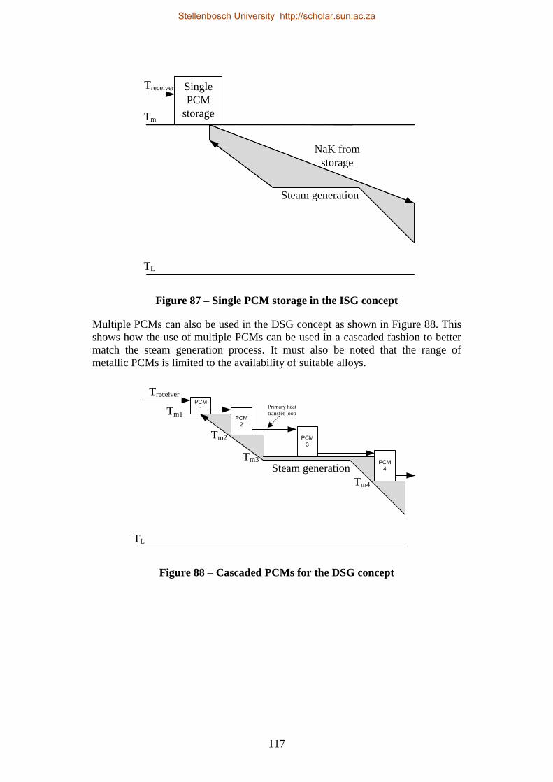
117

Tm

TL

Steam generation

NaK from

storage

Treceiver Single

PCM

storage

Figure 87 – Single PCM storage in the ISG concept

Multiple PCMs can also be used in the DSG concept as shown in Figure 88. This

shows how the use of multiple PCMs can be used in a cascaded fashion to better

match the steam generation process. It must also be noted that the range of

metallic PCMs is limited to the availability of suitable alloys.

TL

Steam generation

TreceiverPCM

1

PCM2

PCM3

PCM4

Primary heat

transfer loopTm1

Tm2

Tm3

Tm4

Figure 88 – Cascaded PCMs for the DSG concept


118

9 HIGH TEMPERATURE CORROSION OF ALSI12

During testing it was discovered that liquid aluminium alloys are extremely

corrosive to most metals and metal oxides (Deqing, 2008). This came as a surprise

since high temperature aluminium corrosion was never mentioned by other

authors who worked on AlSi12 as a storage material (He, et al., 2001) (Li, et al.,

2011) (Wang, et al., 2004). The mechanism of corrosion is diffusion of the other

metal into the molten aluminium alloy (Bouayad, et al., 2003). An electron-

micrograph of the interface between iron and molten aluminium is presented in

Figure 89. This was the result of a sample of polished iron submerged into molten

aluminium at 800 ⁰C for 5 minutes. It is clear that the aluminium and the iron mix

to form an alloy on the boundary interface, and as this process continues, the

aluminium will completely dissolve the iron. The Al-Fe eutectic system is shown

in Figure 90.

Figure 89 - Microstructure of inter-metallic zone (Bouayad, et al., 2003)


119

Figure 90 - Aluminium-iron eutectic system

All corrosion testing that could be found in literature was performed above

700 ⁰C9, and the kinetics of the corrosive process has been measured up to

1000 ⁰C (Bouayad, et al., 2003). The speed of the corrosion process is

proportional to temperature and is influenced by the exact composition of the

alloys. Unfortunately no corrosion tests could be found below 700 ⁰C. The lowest

temperature on the Al-Fe eutectic system is 660.4 ⁰C, but the effect of a lower

melting point Al-Si eutectic system in the presence of iron could not be found.

Regardless, the risk of a rupturing storage vessel merited an immediate halt to the

testing in the steel cylinder which has been used in this project.

In practice there are several corrosion resistant materials that have been

researched. Ceramic materials like; aluminosilicate, refractories, AlN, Al2O3,

Si3N4, TiB2 and sialons (Yan, 2001) (Jensen, et al., 2008). Unfortunately ceramics

are brittle and expensive, and are not well suited for a containment vessel or a heat

exchanger. Boronized carbon steel showed fair resistance to corrosion, but it is not

corrosion proof, and therefore it is not well suited for long term hardware (Tsipas,

et al., 1998). The only feasible corrosion protection that could be found was the

surface treatment of steel by first hot dipping the steel into molten aluminium at

elevated temperatures to form a layer of bonded aluminium-iron alloy, and then to

oxidize the surface of the aluminium (Deqing, et al., 2003). Figure 91 shows an

9 (Deqing, 2008) (Bouayad, et al., 2003) (Deqing, et al., 2003)


120

electron micrograph of surface treated steel that has been exposed to molten

aluminium at 750 ⁰C for 250 hours. It showed excellent corrosion resistance.

Unfortunately this was only a limited experimental run, and further testing is

needed regarding the stability and the toughness of the Al2O3 layer that is giving

the corrosion resistance.

Figure 91 - Electron-micrograph of a surface treated steel sample after

corrosion testing (Deqing, et al., 2003)

Further research is required into the corrosive effects of AlSi12 and other PCMs

on ferrous alloys and methods to provide corrosion protection to these alloys. The

aluminized steel with the oxide layer seems to be a promising technique, but

requires further development and validation for long term use in a large storage

system.


121

10 TECHNO-ECONOMIC FEASIBILITY

The economic feasibility of the storage system is dependent on:

Cost of storage materials

Cost of the containment vessel

Cost implications in the rest of the system:

Savings on heliostats

Cost of the power block

Two-tank molten salt storage is used as a benchmark for cost, as this is the current

state of the art. According to a leading salt producer, SQM, eutectic nitrate salt

mixture (60 % NaNO3 and 40 % KNO3), delivered to a South African port costs

830US$ per metric ton (SQM, 2013). The material cost of salt storage is

calculated and presented in Table 36 as 7.57 US$/kWh. Additionally, the cost of a

two tank molten salt storage system is estimated as 22US$/kWh on top of material

costs (Kolb, et al., 2011).

Table 36 – Material cost of eutectic nitrate salt

Cold storage point 240 °C

Maximum operating temperature 565 °C

Specific heat capacity 1.21 kJ/kg.K

Cost 830 US$/ton

Storage capacity 109.59 kWh/ton

Storage cost 7.57 US$/kWh

No indication of the cost of liquid metal heat transfer equipment, pumps and

steam generators could be found. Looking at liquid metal technology, austenitic

stainless steels offers adequate corrosion resistance to alkali metals, where

corrosion protection for other liquid metals such as lead bismuth eutectic is more

complex (Liquid metal engineering center, 1972).

The ISG concept requires a water-NaK steam generator. This technology has been

proven in the nuclear industry, and has been implemented in some power plants

since 1980, like the BN-600 reactor in Zerechny Sverdlovsk Oblast, Russia. The

BN-600 reactor has a good safety record, and larger reactors are under

construction (World Nuclear News, 2012). The heat transfer equipment, steam

generators, corrosion protection and operation in a solar power plant would be

very similar to that of a nuclear power plant, but with less risk because there is no

nuclear power. Close examination of NaK and Sodium design and handling

protocols would suggest that hardware would not be more complicated than

molten salt systems, even though a higher degree of safety is required (Liquid

metal engineering center, 1972). However, it is not possible to extrapolate cost

data for liquid metal cooling from the nuclear industry to CSP, since the nuclear

systems have much more stringent safety requirements, and liquid metal cooling

would have to be specifically designed for CSP. In this cost analysis it is assumed

that the use of NaK would not directly impact the LCOE.


122

The corrosion protection discussed in chapter 9 does not appear to add significant

additional costs to a CSP system as the corrosion protection only involves the hot

dipping of the heat exchanger pipes and the oxidation of the surface. It is assumed

that the containment structures would cost the same as those used in molten salt

storage. Consequently 22 US$/kWh will be added to the cost of the PCM to serve

as a comparison of overall storage system cost. This is a crude assumption, but

can only be improved if a more detailed study is done.

The material price of AlSi12 is 22.5 R/kg (Zimalco, 2013). At an exchange rate of

11.01 US$/R, this relates to 2.04 US$/kg. The cost of the other alloys had to be

calculated based on the prices of the constituents of the alloys which is

summarised in Table 37.

Table 37 – Constituent metal prices

Cost

(US$/ton) Source

Aluminium 1671 (InvestmentMine, 2014)

Antimony 9200 (InvestmentMine, 2014)

Calcium 2950 (Alibaba, 2014)

Copper 7174 (InvestmentMine, 2014)

Magnesium 2850 (InvestmentMine, 2014)

Silicon 2100 (Alibaba, 2014)

The cost of a number of metallic PCMs from Table 46 (Appendix A) is presented

in Table 38 below. Copper alloys were ignored because of the high cost and low

heat of fusion of these copper alloys. The material cost of these alloys has been

plotted against temperature in Figure 92.

Table 38 – Material cost of a select number of metallic PCMs

°C kJ/kg US$/ton US$/kWh

Si56Mg44 946 757 2430.00 11.56

Si49Mg30Ca21 865 305 2503.50 29.55

Mg47Si38Zn15 800 314 2438.40 27.96

Mg84Ca16 790 272 2866.00 37.93

Al 660 321 1671.00 19.28

Al88Si12 577 560 2043.60 13.14

Mg34.6Al65.4 497 285 2078.93 26.26

Al86.4Si9.4Sb4.2 497 471 2027.54 15.50

Al59Mg35Zn6 443 310 2103.75 24.43

Zn96Al4 381 138 1992.60 51.98

Mg46.3Zn53.7 340 185 2396.77 46.64


123

Figure 92 – Material cost of metallic PCMs versus melting temperature.

Table 39 shows the estimated cost of storage when tanks and heat exchangers are

added to the material cost.

Table 39 – Overall cost estimates of metallic PCMs

°C

Estimated

overall system

cost

(US$/kWh)

%

Increase

in cost

Nitrate salt 565 30 0.00

Si56Mg44 946 33.99 13.30

Al88Si12 577 35.57 18.57

Al86.4Si9.4Sb4.2 497 37.93 26.43

Al 660 42.58 41.93

Al59Mg35Zn6 443 46.86 56.20

Mg34.6Al65.4 497 48.69 62.30

Mg47Si38Zn15 800 50.39 67.97

Si49Mg30Ca21 865 51.98 73.27

Mg84Ca16 790 60.36 101.20

Mg46.3Zn53.7 340 69.07 130.23

Zn96Al4 381 74.41 148.03

AlSi12

(577, 13.14)Si56Mg44

(946, 11.56)

Si49Mg30Ca21

(865, 29.55)

Mg47Si38Zn15

(800, 27.96)

Mg84Ca16

(790, 37.93)

Al86Si9Sb4

(497, 26.26)

Mg34.6Al65.4

(497, 15.50)

Al59Mg35Zn6

(443, 24.43

Zn96Al4

(381, 51.98)

Mg46.3Zn53.7

(340, 46.64)

Al

(660, 19.28)

0

10

20

30

40

50

60

300 400 500 600 700 800 900 1000

Sto

rag

e m

ate

ria

l co

st (

US

$/k

Wh

)

Temperature ( C)


124

All of the metallic PCMs considered here are more expensive than solar salt in its

current form, though some of them are only marginally more expensive. The

impact that metallic PCMs have on the entire CSP plant needs to be considered in

terms of LCOE reduction. To make a reasonable estimation, the current cost

breakdown as outlined by Kolb, et al. (2011) (Table 1, p4) will be used as a basis

for analysis.

Another aspect that needs consideration is the fact that these metallic PCMs are

only some of the eutectic systems that have been investigated, and it is very

possible that there may be many more alloys that are even better suited as PCMs.

This is discussed in section 11.3. Generally the aluminium, silicon, magnesium

and zinc alloys seem to offer great prospective PCMs because of their low cost,

high thermal conductivity and high heat of fusion. It is reasonable to expect that a

range of new metallic PCMs will be Aluminium-Silicon based alloys. Therefore

the estimated total price of AlSi12 storage will be used in the cost analysis (33.99

US$/kWh).

As metallic PCMs are generally more expensive than salts, it is only merited with

the use of a supercritical or an ultra-supercritical steam cycles. Live steam

conditions of 27MPa/600 °C and a 60MPa/620 °C re-heat are normal for

supercritical steam cycles (Cziesla, et al., 2009). The typical thermal efficiency of

such a supercritical steam cycle can be between 45 % and 49 % depending on the

cooling system used. Assuming a 45 % thermal efficiency for a supercritical

power block (Cziesla, et al., 2009), the cost savings on the heliostat field and

storage system can be calculated. A 45 % thermal efficiency is a 7 %

improvement on the 38 % thermal efficiency of current subcritical power cycles,

this is a 15.56 % reduction in energy consumption. This means 15.56 % less

heliostats and storage material. The installation cost of a modern supercritical

steam cycle is 2 % more expensive than a subcritical steam cycle (Bugge, et al.,

2006).

The reduction of LCOE was based on the projected 2013 cost breakdown of

power tower technology by Power tower technology roadmap and cost reduction

plan (Kolb, et al., 2011). They calculated a LCOE of 16.5 US$ cents per kWh for

2013 on a 100 MWe plant with 9 hours of storage. The cost breakdown was

presented in Table 1, p4. In Table 40 below, the effect of such an increase of

thermal efficiency on LCOE is shown, and it shows that a 2.96 % cost reduction is

possible with the use of a supercritical steam cycle and metallic PCMs (Kolb, et

al., 2011).


125

Table 40 – Predicted reduction in LCOE

Cost breakdown

of LCOE

(All costs)

Current cost

breakdown

Breakdown

of 2013

LCOE

US$c

Effect of

storage cost

increase

Effect of

supercritical

steam cycle

Breakdown

of cost with

metal PCM

storage

US$c

Heliostats: 22.10 % 3.65 0.00 % -15.56 % 3.08

Indirect costs: 20.80 % 3.43 0.00 % 0.00 % 3.43

Operations and

maintenance: 12.10 % 2.00 0.00 % 0.00 % 2.00

Power plant: 12.10 % 2.00 0.00 % 2.00 % 2.04

Receiver: 10.10 % 1.67 0.00 % 0.00 % 1.67

Tax: 8.10 % 1.34 0.00 % 0.00 % 1.34

Storage: 7.40 % 1.22 18.75 % -15.56 % 1.26

Balance of plant: 4.00 % 0.66 0.00 % 0.00 % 0.66

Site cost: 2.00 % 0.33 0.00 % 0.00 % 0.33

Tower: 1.30 % 0.21 0.00 % 0.00 % 0.21

Total: 16.51 16.02

Effect on LCOE: -2.96 %

Consequently, the use of metallic phase change materials offers a prospective cost

reduction. Unfortunately the 2.96 % that has been calculated is a crude estimation

at best, but it shows that the use of metallic phase change materials does enable

the use of a supercritical steam cycle, which in itself is the only aspect that

reduces LCOE.

An aspect that needs to be considered is the role of a CSP plant. In the current

environment, CSP has most value to add as a peaking solution. Unfortunately

subcritical steam cycles offer greater flexibility when it comes to transient

conditions than supercritical steam cycles (Heselton, 2005). So it can be argued

that metallic PCM storage with supercritical steam power cycles will most

probably only be beneficial if the CSP plant is designed to deliver base load

power. For base load power to be feasible, the DOE target of 6 US$ cents per

kWh must be achieved. According to the Power Tower roadmap and cost

reduction plan (Kolb, et al., 2011) this would require extensive cost reduction on

all aspects of the plant, including storage and heat transfer equipment. This might

make metallic PCMs and liquid metal heat transfer unfeasible for the whole plant,

since it is more expensive than molten nitrate salt storage.

The use of two tank molten nitrate salt storage in conjunction with cascaded

PCMs could offer a thermal energy storage solution that offers high temperature

storage, while minimizing entropy generation. Such an arrangement is illustrated

in Figure 93, with a T-s diagram in Figure 94.


126

Ts

Supercritical

steam

Molten nitrate salt

from storage

T salt receiver Hot

Storage

TNaK_receiver

PCM

1Tm1

PCM

2

Cold

Storage

PCM

2Tm3

Tm2

Figure 93 – Single metallic PCM storage to enable supercritical steam

100

200

300

400

500

1 2 3 4 5 6 7

7

5

9

Tem

per

ature

(°C

)

8

600

4

1

2

36

270bar

60bar

Figure 94 – T-s diagram of a supercritical steam cycle for combined storage

To evaluate this idea, the Lüen Ultra-supercritical steam power plant is used as a

basis (Cziesla, et al., 2009). The assumption is made that the molten nitrate salt

storage will only be able to heat the steam up to 540°C, and that the metallic PCM


127

storage will heat the steam up to the temperature required by the power cycle. The

steam conditions at the points marketed on the T-S diagram in Figure 94 is

presented in Table 41. The enthalpy differences across heat exchangers are also

calculated, and it is shown that the heat transfer from molten nitrate salt to the

power cycle is 2373.58 kJ/kg, and the heat transfer from metallic PCM to the

power cycle is 164.63 kJ/kg. Therefore only 13.10 % of the energy is supplied by

metallic PCM storage, and 86.9 % of the storage is two-tank molten nitrate salt

storage.

Table 41 – Enthalpy of steam in a supercritical steam generator

Enthalpy:

(kJ/kg)

Heating

provided

by salt

storage:

(kJ/kg)

Heating

provided by

metallic

PCM

storage

(kJ/kg)

(1) Feedwater

conditions

270 bar/

310 °C 1381.50

1899.74

(2) Exit of salt

steam generator:

270 bar/

540 °C 3281.24

193.26

(3) Live steam

conditions:

270 bar/

600 °C 3474.50

(4)

HP turbine

outlet

conditions:

60bar/

350 °C 3043.43

473.84

(5) Exit of salt re-

heater:

60 bar/

540 °C 3517.27

164.63

(6) Re-heat steam

conditions:

60 bar/

610 °C 3681.90

2373.58 357.89

Thus, most of the storage will be done using tried and tested, low cost two-tank

molten nitrate salt storage, and the only value addition is done by replacing

13.10 % of the storage capacity with metallic PCM storage to facilitate the use of

a supercritical steam cycle. Such an implementation would require the use of both

a salt receiver and a liquid metal receiver, and the full cost implications are still

not well understood.


128

11 FUTURE WORK

This project is considered a first step towards higher thermal energy storage in

metallic PCMs and a number of future studies are needed before a conclusive

decision could be made on the feasibility of latent heat storage in metallic PCMs.

This section outlines a number of future research projects that will be needed for

future developments.

11.1 Axial conduction and CFD models

In this project a simplifying assumption was made by ignoring the effects of axial

conduction within the solidifying PCM and not considering the simultaneous

charging and discharging of two heat exchangers in one melt. This was done to

focus on the validity of the Stefan condition applied to metallic PCMs. This would

require CFD techniques, which fell outside the scope of this project.

Axial conduction would be especially important in instances where there is a large

variation of heat transfer rates along the length of the heat exchanger. Therefore it

needs to be taken into consideration in all applications where the heat transfer

fluid’s bulk mean temperature is close to that of the PCM melting point and there

is a significant difference between the inlet and outlet temperature of the heat

transfer fluid.

11.2 Material testing

In chapter 4 it became clear that there is a shortage of high temperature material

properties close to the melting point of AlSi12. Some assumptions proved to be

valid, but high temperature materials testing must be performed on a selection of

prospective metallic PCMs. The most important PCMs are:

Si56Mg44

AlSi12 (LM6)

Al86.4Si9.4Sb4.2

Al

Al59Mg35Zn6

Mg34.6Al65.4

Mg47Si38Zn15

These are the most cost effective metallic PCMs, and cover a range of

temperatures.

The material properties should be measured close to the melting point of the alloy,

in both the liquid and solid phase. The following properties should be known:

Melting point

Heat of fusion

Sub-cooling

Thermal conductivity

Specific heat capacity


129

Density

Coefficient of expansion

Expansion on at phase change

The melting point, heat of fusion, sub-cooling and specific heat capacity can all be

measured using a DSC machine with vacuum capabilities, as sample oxidation

severely affects the DSC measurements even with nitrogen cover. Furthermore,

the use of a DSC curve would be useful in CFD simulation of solidification

process.

The cyclic stability of the metallic PCM should also be evaluated by cycling a

sample through its melting point for about 8000 times, which will be equal to a bit

more than 20 years of operation. Other aspects affecting the stability of the

storage material should also be investigated.

11.3 More alloys and investigation into hyper-eutectics

The use of hyper-eutectic alloys should also be investigated. Material stability

may be prohibitive, but if it is possible to overcome cyclic stability, hyper-eutectic

alloys will be able to provide thermal energy storage at design temperatures,

which will be a great advantage from an exergetic point of view.

Furthermore it is likely that there are more alloys that offer higher heats of fusion

at other melting temperatures that might be more suitable for thermal energy

storage than those identified in this project (Birchenall, et al., 1979).

11.4 High temperature corrosion resistance, heat exchangers and

containment

Much work is still needed on corrosion resistance against molten metals. The

methods discussed in chapter 9 had limited testing, and long term corrosion

resistance must still be verified. The oxidation of aluminized steel is the most

promising corrosion protection method, but the longevity of the oxide layer

through thermal cycles needs to be verified, and the industrial application of this

corrosion resistance need more research.

11.5 The use of liquid metals in CSP

The use of NaK, sodium and other liquid metals as HTFs is well known in the

nuclear industry and its advantages in CSP is very clear. Safety, design and

material handling protocol are well established in the nuclear industry, but will

need to be adapted for CSP to reduce the cost. A detailed study is required on the

application of liquid metal heat transfer to CSP. The main questions regarding

liquid metal heat transfer in CSP is economic feasibility and safety. This includes

the use of LBE, NaK and sodium.


130

11.6 Analysis of a combined molten salt storage system with metallic PCM

storage

The concept of combining two-tank molten nitrate salt storage and metallic PCM

in a cascaded fashion is new. This may be a key to the implementation of

supercritical steam power cycles into CSP to deliver base load power. This

concept must be investigated further and an in-depth techno-economic study

needs to be performed. Most likely the concept will require two receivers, one

salt, and another for liquid metal.

11.7 Optimisation through entropy minimization

In section 8.6.2 the importance of entropy minimization is highlighted. A detailed

study of metallic PCM storage and entropy minimization should be done. The

Flownex model developed in chapter 8 can be used as a base to work from.


131

12 CONCLUSION

The current state of the art thermal energy storage is two tank molten salt. This

has a maximum operational temperature of 565 °C, limited largely by the thermal

properties of nitrate salts. This limits the source temperature of the power cycle,

and bounds the power cycle to a subcritical steam cycle of which the maximum

thermal efficiency is 36 to 40 %. Higher efficiency power cycles (like

supercritical steam) offer significant reductions in the levelised cost of electricity

(LCOE), but these power cycles require higher source temperatures than currently

possible with conventional two tank molten salt storage.

Phase change materials (PCMs) offer higher temperature energy storage than

possible with sensible heat storage. Metallic PCMs have thermal properties that

are more favourable than those of non-metallic phase change materials, with high

thermal conductivity and low sub-cooling being the most significant. The central

topic and contribution of this project was to evaluate the feasibility of metallic

PCMs as storage materials that could increase the maximum possible thermal

energy storage temperature to enable higher efficiency power generation. The

application of metallic PCMs in concentrating solar power is a novel idea, and the

feasibility of metallic PCMs had to be evaluated.

Key to the implementation of metallic PCMs are high temperature HTFs. Liquid

metals are the only heat transfer fluids (apart from gasses) that can operate at

temperatures suitable for supercritical steam and thermal energy storage (TES) in

metallic PCMs. Liquid metal receivers can absorb solar flux densities more than

twice those possible with other heat transfer fluids. This results in compact, high

efficiency receivers, which is extremely advantageous at high temperatures.

Additionally, the eutectic sodium-potassium alloy (NaK) has a melting point of

-12.8 °C which means that there is no need for trace heating in the primary heat

transfer loop. This significantly increases safety in the liquid metal system, as it is

possible to drain the heat transfer loop with no risk of pipe blockage. For this

reason, NaK was chosen as the heat transfer fluid used in this study.

To evaluate the idea of using liquid metal HTFs and metallic PCMs together, two

storage concepts have been developed. Aluminium-Silicon (AlSi12) was

identified as an ideal metallic PCM for research and the analytical work was

based on concepts employing both NaK and AlSi12, one where steam is generated

directly from the PCM and another where the steam generation is done using a

NaK-water heat exchanger.

Core to the analysis of latent heat thermal energy storage is the moving boundary

heat transfer problem in a cylindrical coordinate system, associated with the

solidification and melting of a PCM around a cylindrical pipe. Through an

experiment it was found that the Stefan condition holds true for AlSi12, which

allows analysis by quasi steady heat transfer assumptions. This allowed for the

development of a discretised transient model using an enthalpy tracking method to

predict the movement of a moving boundary. Because the Stefan condition is met,

an instantaneous heat transfer analysis can be done using a standard resistance


132

model on the moving boundary to calculate heat transfer rates. This is especially

convenient for heat exchanger sizing.

A prototype thermal energy storage unit was built, and it was used to validate the

assumptions made regarding the moving boundary heat transfer problem. It was

possible to predict the movement of the moving boundary and it was shown that

the Stefan condition holds true even for very high temperature gradients between

the coolant and the PCM. Furthermore, it was shown that instantaneous heat

transfer calculations could be used to design the heat transfer surfaces in such a

storage unit.

It must be noted that the effect of axial conduction was ignored, and only radial

conduction was considered in this model. The effect of axial conduction will have

to be analysed in detail using CFD techniques and thus fell outside the scope of

this project.

To demonstrate and evaluate the concept, a Flownex model was built based on a

subcritical steam power cycle. The thermodynamic model of the power generating

cycle yielded boundary conditions which were used for the sizing of the heat

exchangers in the storage system and steam generators. An integrated model of

the storage system, primary heat transfer loop and the power block yielded a

model that can be used in future studies.

The evaluation of the concepts highlighted that the DSG concept had a number of

issues relating to entropy generation, practical implementation, process control

and start-up and shutdown procedures. The ISG concept proved more favourable

in many respects, but requires a liquid metal-water heat exchanger. If NaK or

sodium were used as a primary HTF, the safety and cost of the steam generator

may be prohibitive, and requires further investigation. Alternative metallic HTFs

such as eutectic lead-bismuth alloy (LBE) may also offer solutions, especially in

applications where the plant is used for base load energy production.

One of the key problems with the use of latent heat thermal energy storage is the

fact that isothermal storage is responsible for entropy generation. Heat transfer

between sensible heat and latent heat inherently yields some entropy generation,

both in the primary heat transfer loop, and towards the working fluid of the power

cycle. The use of cascaded PCMs can minimize entropy generation. This is a topic

that needs further investigation.

During a techno economic evaluation, it was determined that metallic PCMs will

add value to a CSP plant by enabling the use of supercritical steam power cycles.

However, this is only significant if the DOE target for LCOE of 6US$c/kWh is

reached for the entire plant, which will allow CSP to compete for base load

generation. To reach this target cost reduction will have to be performed on the

entire plant, and the use of high temperature storage will only form one part of the

cost reduction solution.

The benefit of using metallic PCMs on their own is apparent, but storage costs can

further be reduced by using metallic PCM storage in conjunction with traditional

two tank molten nitrate salt storage, as only 13.10 % of the storage needs to be at


133

temperatures above that of the two tank molten salt storage. This also has benefits

from an entropy minimization point of view. Pure aluminium, eutectic

magnesium-aluminium alloy, eutectic aluminium-silicon alloy and eutectic

silicon-magnesium alloy seem to be promising metallic PCMs, although more

metallic PCMs need to be identified to enable cascaded PCMs across a greater

temperature range and at smaller increments for entropy minimization.

Furthermore, aluminium and aluminium alloys are highly corrosive, and

appropriate corrosion protection needs to be developed for industrial applications.

Oxidation of aluminized steel surfaces appears to be a viable corrosion protection

technique, but the application of this technique and the longevity of the corrosion

resistance still need more investigation.

The use of liquid metal HTFs in CSP also need further investigation, as it is

central to the development of high temperature thermal energy storage.

Experience gained from the implementation of liquid metals in the nuclear

industry will serve as a good basis, but the application to CSP needs to be fully

understood, and cost reduction needs to be kept in mind.


134

13 REFERENCES

Achenbach, T. 2011. Development of an edge module for open volumetric

receiver for the use of the radiation at the receiver boundary region

[Conference] // SolarPACES. - Granada

Adinberg, R., Zvegilsky, D. & Epstein, M. 2010 Heat transfer efficient thermal

energy storage for steam generation [Journal] // Energy conversion management,

51 pp. 9-15.

Agyenim, F. Hewitt, N. Eames, P. & Smyth, M. 2009. A review of materials,

heat transfer and phase change problem formulation for latent heat thermal

energy storage systems (LHTESS) [Journal] // Renewable and sustainable energy

reviews. 14(2) pp. 615-628

Alibaba.com [Online]. Available: http://www.alibaba.com/. – [12 February

2014]

Allen, K.G. Kröger, D.G. & Fluri, T.P. 2009. Thermal energy storage in a rock

bed [Conference] // ISES. - Johannesburg : ISES

Battleson, K.W. 1981. Solar Power Tower Design Guide: Solar thermal central

receiver power systems, a source of electricity and/or process heat [Report] :

Design guide. - : Sandia national labs - Albuquerque

Bejan, A. 1982. Entropy generation through heat and fluid flow [Book]. - New

York : Wiley

Bejan, A. 1995. Entropy generation minimization [Book]. - Boca Raton : CRC

press

Bejan, A. 1996. Method of entropy generation minimization, or modelling and

optimization based on combined heat transfer and thermodynamics [Journal] //

Revue Generlae de Thermique. 35. pp. 637-646.

Birchenall, C. E. & Reichman A.F. 1979. Heat storage in Eutectic Alloys

[Journal]. - Delaware : Metalurgical Transactions A, Vol 11 A.

Bird, R.E. & Hulstrom, R.L. 1981. Simplified Clear Sky Model for Direct and

Diffuse Insolation on Horizontal Surfaces [Report] : Technical Report No.

SERI/TR-642-761. – NREL - Golden (CO)

Bouayad, A. Gerometta & C. Belkebir, A. 2003. Kinetic interactions between

solid iron and molten aluminium [Journal] // Materials Science and Engineering. -

A363, pp.53-61/

Brandes, E.A. & Brook G.B. 1998. Smithells Metals Reference Book (7th

Edition) [Book]. - Oxford : Butterworth-Heinemann.

Bugge, J. Kjaer, S. & Blum, R. 2006. High-efficiency coal-fired power plants

development and perspectives [Journal] // Energy 31. pp. 1437-1445

Burch S D [et al.]. 1996. Applications and benefits of catalytic converter thermal

management [Conference] // SAE Fuels & Lubricants spring meeting. -

Dearborn,(MI) : SAE.


http://www.alibaba.com/

135

Cengel, Y.A. & Boles, M.A. 2002. Thermodynamics: an engineering approach -

fourth edition [Book]. - New York : McGraw-Hill.

Cengel, Y.A. 2003. Heat transfer - A practical approach [Book]. - New York :

Mc Graw Hill.

Chambadal, P. 1957. Les centrales nucléaires [Journal] // Armand Colin. pp.1-

58.

Coastal Chemical 2011. Hitec Solar Salt [Report] Houston : Coastal Chemical .

Coastal Chemical 2012. Hitec heat transfer salt [Report] Houston : Coastal

Chemical .

Cziesla, F. Bewerunge, J. & Senzel, A. 2009. Lünen – state of the art

supercritical steam power plant under construction [Conference] // POWER-GEN

Europe 2009, Cologne.

Darcy, H. 1857. Recherches Experimentales Relatives au Mouvement de L'Eau

dans les Tuyaux [Book]. - Paris : Mallet-Bachelier

Deqing, W. 2008. Phase evolution of an aluminized steel by oxidation treatment

[Journal]. - Dalian : Applied Surface Science, 2008. – 254 pp.3026–3032.

Deqing, W. Ziyuan, S. & Longjiang, Z. 2003. A liquid aluminium corrosion

resistance surface on steel substrate [Journal] // Applied Surface Science. -

214pp. 304-311.

Dostal, V. Driscoll, M.J. & Hejzlar, P. 2004. A Supercritical carbon dioxide

cycle for next generation nuclear reactors [Report] : PhD Thesis. - Boston : MIT.

Dow chemical company. 2001. Product information: Dowtherm A - Synthetic

organic heat transfer fluid, [Report] Dow chemical company

Eck, M [et al.] 2011. Direct steam generation in parabolic troughs at 500degC-

First results of the REAL-DISS project [Conference] // SolarPACES - Granada

Flownex 2011. Flownex theory manual [Book]. - Pretoria : Flownex,

Fluri, T.P. 2009. The potential of concentrating solar power in South Africa

[Journal] // Energy Policy (37). pp. 5075-5080.

Geosun Africa [Online]. Available: geosun.co.za. [29 August 2013]

Getling, A.V. 1998. Rayleigh-Benard Convection: Structures & Dynamics

[Book]. - London: World Scientific Publishing.

Gil A [et al.] 2010. State of the art on high temperature thermal energy storage

for power generation. Part 1 - Concepts, materials and modellization [Journal]. -

Lleida : Renewable and Sustainable Energy Reviews, 14, pp.1364-1381.

Gnielinski, V. 1975. Neue Gleichungen Für den Wärme- und den Stoffübergang

in durbulent durchströmten Rohren und Kanälen [Journal] // Forschung im

Ingenieurwesen A. 41(1) pp 8-16.


136

Hall A, Ambrosini A & Ho C. 2012. Solar Selective Coatings for Concentrating

Solar Power Central Receivers [Journal] // Advanced materials and processes. pp.

28-32.

He, Q. and Zhang, W. 2001 A study on latent heat storage exchangers with the

high-temperature phase-change material [Journal]. - Wuhan : International journal

of energy research. pp. 25-30.

Herring, D.H. 2010. Oil Quenching [Report]. Illinois : The Herring group, Inc.

Herrmann, U. Geyer, M. & Kearney, D. 2006 Overview on thermal storage

systems // Workshop on Thermal Storage for Trough Power Plants: FLABEG

Solar International GmbH.

Heselton, K.2005. Boiler Operator's Handbook [Book]. - Lilburn: Fairmont

Press,

Hoshi, A. [et al.] 2005. Screening of high melting point phase change materials

(PCM) in solar thermal concentration technology based CLFR [Journal] // Solar

Energy 79. pp. 332-339

Hummon, M. & Denholm, P. 2012. Simulating the value of concentrating solar

power with thermal energy storage in a production cost model [Report]:

Technical report. - Denver : NREL

International Energy Agency 2010.Technology Roadmap [Report] / IEA. -

Paris : IEA

InvestmentMine. [Online]. Available: http://www.infomine.com – [12 February

2014]

Jensen, M.S. [et al.]. 2008. Degradation of TiB2 ceramics in liquid aluminium

[Journal] // Journal of the European Ceramic Society (28). pp. 3155-3164.

Johnson, W.R. 1998. The Handbook of Fluid Mechanics [Book]. - Heidelberg :

CRC Press LLC

Kakac, S. & Yener,Y. 1993 Heat conduction [Book]. - Washington : Taylor &

Francis

Karassik, I.J. [et al.] 1985. Pump handbook [Book] New York: McGraw-Hill

Kearney, D. Herrmann, U. & Nava, P. 2003. Assessment of molten salt heat

transfer fluid in a parabolic trough solar field [Journal] // Journal of solar Energy

Engineering(125). pp:170-176.

Kenisarin, M.M. 2009. High Temperature Phase Change Materials for Thermal

Energy Storage [Journal]. - Renewable and Sustainable Energy Reviews 14(3).

pp: 955-970

Kolb. G.J. [et al.] 2011. Power tower technology roadmap and cost reduction

plan [Report]. Albuquerque: Sandia national laboratories


137

Kopeliovich, D. Heat transfer oil ISO100 [Online] Available:

http://www.substech.com/dokuwiki/doku.php?id=heat_transfer_oil_iso_100.

[05 July 2013]

Lai, G.Y. 2007. High-temperature Corrosion and Materials Applications

[Book] – New York : ASM International.

Li, F. Hu, Y. & Zhang, R. 2011. The influence of heating-cooling cycles on the

thermal storage performances of Al-17 wt.% Si alloy [Journal]. - Guangdong:

Advanced Materials Research. – pp: 239-242.

Liquid metal engineering centre 1972. Sodium-NaK engineering handbook

Vols. 1-5. [Book]. - New York : Gordon and Breach

Lock, G.S. 1996. Latent heat transfer: An introduction to fundamentals [Book]. -

Oxford : Oxford Science Publication,

Lockheart, R.W. & Martenelli, R.C. 1949. Proposed Correlation of Data for

Isothermal heat transfer in phase change [Journal] // Chem. Eng. Prog. (45), pp:

34-48

Matbase Matbase [Online] Available - http://www.matbase.com/. [9 September

2013]

Medrano, M. [et al.] 2010. State of the art on high-temperature thermal energy

storage for power generation. Part 2 - Case studies [Journal]. - Renewable and

Sustainable Energy Reviews14, pp. 1382-1401

Meduri, P. K. Hannemann, C.R. &Pacheco, J.E. 2013. Performance

characterization and operation of e-solar's sierra sun tower power tower plant

[Conference] // Las Vegas: Solar PACES.

Michels, H. & Pitz-Paal, R. 2007. Cascaded latent heat storage for parabolic

trough solar power plants [Journal] // Solar Energy. - 81. - pp. 829-837.

Mondolfo, L.F. 1976. Aluminium Alloys: Structures and properties [Book]. -

London : Butter Worths

Munn, G. Information on the properties of AlSi12 [Interview]. - 14 February

2013.

Murray, J.L. and McAlister, A. J. 1984. The Al-Si (Aluminium-Silicon) system

[Journal] // Bulletin of alloy phase diagrams pp. 74-84.

Novikov, I.I. 1958. The Efficiency of Atomic Power Stations [Journal] // Journal

Nuclear Energy II. pp. 125–128.

Schiel, W.J. 1988. Testing and external sodium receiver up to heat fluxes of

2.5MW/m2: Results and conclusions from the IEA-SSPS high flux experiment

conducted at the central receiver system of the Plataforma Solar de Almeria

[Journal] // Solar Energy (41) pp. 255-265.

Siemens 2010. Steam turbines for CSP plants [Brochure] - Erlangen: Siemens AG


138

Special Metals Corperation Special metals [Online] Available -

www.specialmetals.com. [14 November 2013]

SPX HT-5--200GPM Tester [Online] Available - http://www.spx.com/en/power-

team/pd-ht-series/ [3 November 2013]

SQM Contact sustainability SQM [Interview]. - 5 September 2013.

Steine, W.B. and Harringan, R.W. 1986. Power from the sun [Book]. - New

York : John Wiley and sons, Inc.

Steiner,D.I. and Taborek, J. 1992. Flow Boiling Heat Transfer in Vertical Tubes

Correlated by an Asymptotic Model [Journal] // Heat Transfer Engineering 13(2)

Stoddard, L. Abiecunas, J. & O'Connell, R. 2006. Economic, Energy, and

Environmental Benefits of Concentrating Solar Power in California [Report]

Subcontract Report. - Battelle: NREL.

Sun, J.Q. [et al.] 2007. Thermal Reliability Test of Al-34%Mg-6%Zn Alloy as

Latent Heat Storage Material and Corrosion of Metal With Respect to Thermal

Cycling [Journal] // Energy Conversion Management (48). pp. 619-624.

Tamme,R. Laing, D. & Steinmann, W.D. 2004. Advanced thermal energy

storage technology for parabolic trough [Journal] // Journal of solar energy

engineering . 126(2) pp. 109-125.

Tamme. R. 2007. Energy storage for direct steam solar power [Conference] //

The DISTOR Project. Consortium–objective–achievements. DISTOR

dissemination workshop. Energy storage for direct steam solar power plants :

Almeria, Spain.

Technical ceramics Ceramic formers spec sheet. - Capetown [5 December 2013]

Technical Glass. Superwool 607 HT. [Online] Available

http://www.goodfellow.com/corporate/news/2011/Superwool-607-HT-

Goodfellow-UK-Sept-2011.pdf [ 01 September 2011]

Tenekedjiev N [et al.] 1995. Microstructure and thermal analysis of strontium-

treated aluminium-silicon alloys [Book]. - Des Plaines : American foundrymen's

Society, Inc.

Thome, J.R. Kattan, .N and Ould Didi, M. B. 2002. Prediction of two-phase

pressure gradients of refrigerants in horizontal tubes [Journal] // International

Journal of Refrigeration 25(7). pp. 935-947.

Torresol Energy Newspaper library [Online] Available

http://www.torresolenergy.com/EPORTAL_DOCS/GENERAL/SENERV2/DOC-

cw524d4f94e5bff/gemasolar-celebrates-its-second-anniversary-with-an-excellent-

operational-record.pdf. [ 26 September 2013]

Tsipas, D.N. [et al.] 1998. Degradation behaviour of boronized carbon and high

alloy steels [Journal] // Material Letters (37). pp. 128-131.


http://www.specialmetals.com/

http://www.spx.com/en/power-team/pd-ht-series/

http://www.spx.com/en/power-team/pd-ht-series/

http://www.goodfellow.com/corporate/news/2011/Superwool-607-HT-Goodfellow-UK-Sept-2011.pdf

http://www.goodfellow.com/corporate/news/2011/Superwool-607-HT-Goodfellow-UK-Sept-2011.pdf

http://www.torresolenergy.com/EPORTAL_DOCS/GENERAL/SENERV2/DOC-cw524d4f94e5bff/gemasolar-celebrates-its-second-anniversary-with-an-excellent-operational-record.pdf



139

U.S. Energy Information Administration 2012. Annual Energy Outlook 2012 -

with Projections to 2035 [Report] : Independent report. Washington : U.S. Energy

Information Administration,

Voller, V. and Cross, M. 1980 Accurate solutions of moving boundary problems

using the enthalpy method [Journal] // International journal of heat and mass

transfer (24). pp. 545-556.

Voller, V. and Swaminathan, C.R. 1992. A general enthalpy method for

modelling solidification process [Journal] // Metallurgical transactions B

(23B). pp. 651-664.

Wagner, W. [et al.] 1997. The IAPWS Industrial Formulation 1997 for the

thermodynamic properties of water and steam [Journal] // Journal of Engineering

for Gas Turbines and Power (122) - pp. 150-182.

Wang, X. [et al.] 2004. Experimental research on a kind of novel high

temperature phase change storage heater [Journal]. - Beijing: Energy conversion

and management.

Weisbach, J. 1845. Lehrbuch der Ingenieur- und Maschinen-Mechanik [Book]. -

Braunschwieg : Paris.

World Nuclear News Large fast reactor approved for Beloyarsk [Online].

Availeble : http://www.world-nuclear-news.org/NN-

large_fast_reactor_approved_for_Beloyarsk-2706124.html. 27 June 2012

Yan, M. 2001. Durability of materials in molten aluminium alloys [Journal] //

Journal of materials science (36). pp. 285-295.

Zimalco Delivery of unit [Invoice]. - 17 January 2013.


http://www.world-nuclear-news.org/NN-large_fast_reactor_approved_for_Beloyarsk-2706124.html

http://www.world-nuclear-news.org/NN-large_fast_reactor_approved_for_Beloyarsk-2706124.html

140

APPENDIX A CANDIDATE PHASE CHANGE MATERIALS

Table 42 – Carbonates (Kenisarin, 2009)

Material Tm (°C) λ (J/g)

Na2CO3(6.4)–85.8NaOH–7.8NaCl 282 316

Li2CO3(32.1)–34.5K2CO3–33.4Na2CO3 397 276 Li2CO3(47)–53K2CO3 488 342

Li2CO3(47)–53K2CO3 491 321

Li2CO3(44)–56Na2CO3 496 370 Li2CO3(28)–72K2CO3 498 263

Li2CO3(28.5)–71.5K2CO3 498 316 Li2CO3(44.3)–55.7Na2CO3 498 393

Li2CO3(35)–65K2CO3 505 344

NaBr(43)–2NaF–55Na2MoO4 506 241 K2CO3(62)–17NaF–21KCl 520 274

Li2SO4(59.8)–36.7Li2MoO4–3.5CaMoO4 538 406

Li2CO3(20)–60Na2CO3–20K2CO3 550 283 KBr(60)–40KF 576 315

KBr(65)–35K2MoO4 625 91

Li2SO4(82)–11.44CaSO4–6.56CaMoO4 680 207 K2CO3(47.8)–52.2K2CO3 710 176

K2CO3(50)–50Na2CO3 710 163

K2CO3(51)–49Na2CO3 710 163

Table 43 – Hydroxides (Kenisarin, 2009)


NaOH(50)–50KOH 169 202

LiOH(30)–70NaOH 210 278

NaOH(20)–80NaNO2 230 206 NaOH(73)–27NaNO2 237 249

NaOH(78.1)–3.6NaCl–18.3NaNO3 242 242

NaOH(28)–72NaNO3 246 182 NaOH(55.6)–4.2NaCl–40.2NaNO3 247 213

NaOH(81.5)–18.5NaNO3 256 251

LiOH(63)–37LiCl 264 437 NaOH(59)–41NaNO3 266 278

NaOH(59)–41NaNO3 266 221

LiOH(65.5)–34.5LiCl 274 339 LiOH(62)–36.5LiCl–1.5KCl 282 300

NaOH(85.8)–7.8NaCl–6.4Na2CO3 282 316

NaOH(88.3)–5.3NaCl–6.4Na2CO3 282 279 NaOH(87.3)–6.1NaCl–6.6Na2CO3 291 283

NaOH(77.2)–16.2NaCl–6.6Na2CO3 318 290


141

Table 44 – Chlorides (Kenisarin, 2009)


LiCl(59.15)–40.85Ca(NO3)2 270 167

NaCl(7.8)–85.8NaOH–6.4NaCO3 282 316 LiCl(54.2)–6.4BaCl2–39.4KCl 320 170

LiCl(47.4–47.7)–(46.8–47.0)KCl–(3.2–3.4)LiCO3–(2.1–2.4)LiF 340 375

LiCl(58)–42KCl 348 170 KCl(28.7)–45MnCl2–26.3NaCl 350 215

LiCl(23.4–24.2)–(24.8–25.3)LiVO3–(27.1–27.6)Li2MoO4–(17.3–17.8)Li2SO4–(6.1–6.2)LiF 360 284 NaCl(22.5–26.5)–(18.5–22.5)KCl–(57.0–53.0) MgCl2 385 405

KCl(21.6)–45.4MgCl2–33.0NaCl 385 284

KCl(45.5)–34.5MnCl2–20NaCl 390 230

KCl(20)–50MgCl2–30NaCl 396 291

KCl(37.7)–37.3MnCl2–25NaCl 400 235

NaCl(56)–44MgCl2 430 320 KCl(54)–46ZnCl2 432 218

KCl(61)–39MgCl2 435 351

NaCl(56.2)–43.8MgCl2 442 325 LiCl(58.5)–23.6Li2SO4–17.9Li2MoO4 445 327

KCl(36)–64MnCl2 448 236

LiCl(49.0)–12.75Li2SO4–38.25LiVO3 449 450 KCl(35)–65MnCl2 450 237

NaCl(60)–40MgCl2 450 328

NaCl(48)–52MgCl2 450 430 CaCl2(47.6)–8.1KCl–41.3NaCl–2.9NaF 460 231

CaCl2(41.6)–2.2KCl–8.8MgCl2–47.4NaCl 460 245

CaCl2(50)–7.25KCl–42.75NaCl 465 245 KCl(36)–64MgCl2 470 388

BaCl2(8.7)–52.3KCl–18.2MgCl2–20.7NaCl 475 248

BaCl2(13.1)–16.9CaCl2–47.3KCl–22.7NaCl 478 208 BaCl2(9.3)–22.2CaCl2–42.7KCl–25.8NaCl 479 217

LiCl(69.5)–26.5LiF–4MgF2 484 157

KCl(25)–27 CaCl2–48 MgCl2 487 342 CaCl2(50)–1.5CaF2–48.5NaF 490 264

CaCl2(52.3–55)–(45–47.2) NaCl 500 239

NaCl(33)–67 CaCl2 500 281 CaCl2(66)–5KCl–29NaCl 504 279

SrCl2(68)–13KCl–19NaCl 504 223

NaCl(5)–40NaBr–55Na2MoO4 524 215 KCl(40)–23KF–37K2CO3 528 283

MgCl2(37)–63 SrCl2 535 239

KCl(28)–19NaCl–53BaCl2 542 221 KCl(24)–47BaCl2–29CaCl2 551 219

NaCl(952)–48NiCl2 573 558

LiCl(94.5)–5.5MgF2 573 131 NaCl(38.5)–23NaBr–38.5Na2MoO4 612 168

CaCl(38.5)–11CaSO4–4CaMoO4 673 224


142

Table 45 – Fluorides (Kenisarin, 2009)


NaF(5)–87NaNO3–8NaCl 288 224

LiF(7.0)–41.5LiCl–16.4LiVO3–35.1Li2CrO4 340 177 LiF(16.2)–51.5LiCl–16.2Li2SO4–16.2Li2MoO4 402 291

LiF(17.6–17.7)–(33.2–33.8) KF–(40.0–40.4) KCO4–(8.6–8.7) KCla 422 412

LiF(20)–80LiOH 427 1163 LiF(25.0)–43.8LiVO3–14.8Li2SO4–16.5Li2MoO4 428 260

LiF(80)–20LiOH 430 528 LiF(45.7)–1.8BaF2–41.2KF–11.3NaF 438 332

LiF(42.5–45.5)–(41.0–43.0) KF–(10.7–11.5) NaF–(2.8–3.0) KCl 440 682

LiF(27.1)–11.9NaF–55.1KF–5.9MgF2a 449 699

LiF(29.2)–11.7NaF–59.1KFa 454 414

LiF(46.5)–42KF–11.5–NaF 454 325

Li(29)–12NaF–59KFa 463 442 LiF(73.6)–26.4LiCl 485 403

KF(50)–50LiCl 487 344

LiF(33)–67KFa 493 458 LiF(18.0)–53.0LiVO3–29.0Li2MoO4 493 297

NaF(20.1)–79.9ZrF4a 510 255

NaF(17)–21KCl–62K2CO3a 520 274

KF(23)–40KCl–37K2CO3a 528 283

LiF(36.1)–34NaF–18.5CaF2–3.3BaF2–8.1BaMoO4 536 653

KF(40)–60KBr 576 315 LiF(25.67–25.76)–(36.45–36.57)NaF–(27.0–27.25) CaF2–(10.63–10.67)MgF2

a 593 510

KF(55)–45KCl 605 407

LiF(35.2)–38.3NaF–26.5CaF2 615 636 LiF(52)–35NaF–13CaF2 615 640

Li(46)–44NaF–10MgF2 632 858

NaF(27)–73NaBr 642 360 LiF(34.51–34.79)–(37.25–37.6)MgF2–(24.5–25.0)CaF2–(3.21–3.31)NaF 651 460

LiF(60)–40NaF 652 816

NaF(33.5)–66.5NaCl 675 572 LiF(62)–19NaF–19MgF2 693 690

LiF(70)–30MgF2 728 520

NaF(65)–23CaF2–12MgF2 743 568 LiF(67)–33MgF2 746 947

LiF(74)–13KF–13MgF2 749 860

LiF(80)–20CeF3 756 500 LiF(81.5)–19.5CaF2 769 820

KF(85)–15CaF2 780 440

KF(85)–15MgF2 790 520 NaF(64)–20MgF2–16KF 804 650

NaF(62.5)–22.5MgF2–15KF 809 543

NaF(68)–32CaF2 810 600 NaF(75)–25MgF2 832 627

CaF2(49)–41.4CaSO4–9.6CaMoO4 943 237


143

Table 46 – Metals (Kenisarin, 2009)


Cu(83)–10P–7Si 840 92

Cu(74)–19Zn–7Si 765 125 Cu (91)–9P 715 134

96Zn–4Al 381 138

Mg(55)–28–17Zn 400 146 Zn(49)–45Cu–6Mg 703 176

Mg(52)–25Cu–23Ca 453 184 46.3Mg–53.7Zn 340 185

Cu(80)–20Si 803 197

Zn2Mg 588 230

Mg2Cu 841 243

Mg(60)–25Cu–15Zn 452 254

Mg(84)–16Ca 790 272 34.65Mg–65.35Al 497 285

Al(54)–22Cu–18Mg–6Zn 520 305

Si(49)–30Mg–21Ca 865 305 Al(59)–35Mg–6Zn 443 310

Mg(47)–38Si–15Zn 800 314

64.3–34.0Cu–1.7Sb 545 331 68.5Al–5.0Si–26.5Cu 525 364

60.8Al–33.2Cu–6.0Mg 506 365

60.8Al–33.2Cu–6.0Mg 506 365 Cu(69)–17Zn–14P 720 368

66.92Al–33.08Cu 548 372

64.1Al–5.2Si–28Cu–2.2Mg 507 374 46.3Al–4.6Si–49.1Cu 571 406

Cu(56)–27Si–17Mg 770 420

Al(65)–30Cu–5Si 571 422 86.4Al–9.4Si–4.2Sb 471 471

83.14Al–11.7Si–5.16Mg 555 485

87.76Al–12.24Si 557 498 Si(56)–44Mg 946 757

Table 47 – Nitrates (Kenisarin, 2009)


LiNO3(29)–17NaNO3–49.4KNO3–4.6Sr(NO3)2a 105 110

LiNO3(33)–67KNO3a 133 170

LiNO3(31.7)–68.3KNO3a 135 136

KNO3(53)–40NaNO2–7NaNO3a 142 80

LiNO3(55.4)–4.5NaNO3–40.1KCla 160 266

LiNO3(58.1)–41.9KCla 166 272

LiNO3(47.9)–1.4LiCl–50.7NaNO3a 180 265

LiNO357)–43NaNO3a 193 248

LiNO3(49)–51NaNO3a 194 265

LiNO3(45)–47NaNO3–8Sr(NO3)2a 200 199

LiNO3(87)–13NaCla 208 369

KNO3(54)–46NaNO3a 222 100

NaNO3(54)–46KNO3 222 117 NaNO3(70)–30NaOH 247 158

LiNO3(97.4)–2.6Ba(NO3)2 253 368

NaNO3(86.3)–8.4NaCl–5.3Na2SO4 287 177


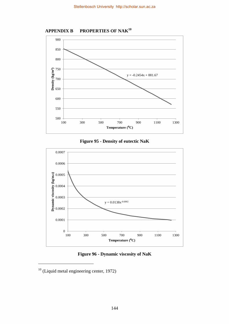
144

APPENDIX B PROPERTIES OF NAK10

Figure 95 - Density of eutectic NaK

Figure 96 - Dynamic viscosity of NaK


y = -0.2454x + 881.67

500

550

600

650

700

750

800

850

900

100 300 500 700 900 1100 1300

Den

sity

(k

g/m

3)

Temperature (⁰C)

y = 0.0138x-0.6902

0

0.0001

0.0002

0.0003

0.0004

0.0005

0.0006

0.0007

100 300 500 700 900 1100 1300

Dy

na

mic

vis

cosi

ty (

kg

/m.s

)

Temperature (⁰C)


145

Figure 97 - Kinematic viscosity of eutectic NaK

Figure 98 - Thermal conductivity of eutectic NaK

y = 8E-06x-0.562

0.E+00

1.E-07

2.E-07

3.E-07

4.E-07

5.E-07

6.E-07

7.E-07

100 200 300 400 500 600 700 800 900

Kin

ema

tic

vis

cosi

ty (

m2/s

)

Temperature (⁰C)

y = -2.2000E-05x2 + 2.0700E-02x + 2.1400E+01

22

22.5

23

23.5

24

24.5

25

25.5

26

26.5

27

100 200 300 400 500 600 700 800 900

Th

erm

al

Co

nd

uct

ivit

y (

W/m⁰C

)

Temperature (⁰C)


146

Figure 99 - Specific heat of eutectic NaK

y = 0.0003x2 - 0.369x + 970.69

850

860

870

880

890

900

910

920

930

940

950

100 200 300 400 500 600 700 800

Sp

ecif

ic h

eat

(J/k

g.⁰

C)

Temperature (⁰C)


147

APPENDIX C DERIVATION OF THE STEFAN NUMBER

This section presents the derivation of the Stefan number as presented in Lock

(1996):

Consider a phase change problem where a phase change material is being frozen

by removing heat from a surface at Y = 0. The initial temeprature of the material

is T∞, the meling point is Ti and the temperature of the surface at Y=0 is T0. This

is shown in figure 100.

T∞

Ti

T0

Freezing

temperature

LiquidSolid

Y Yi

Figure 100 - Temperature profiles during one-dimensional freezing of a

liquid initially at T∞

The conduction in the solid region can be described as:

(C.1)

And similarly for the liquid:

(C.2)

And the interface boundary can be described as:

(

) (

) (C.3)


148

Assuming T∞ > Ti, that all the material was molten at t=0, and that the surface

temperature is suddenly lowered to a fixed value of T0<Ti. From Figure 100 it is

clear that some scales are implied in the liquid (Ti<TL<T∞), solid (T0<TS<Ti) and

a dimensional scale (0<YS<Yi). By designation the scale of a variable by a

superscript c, we take:

And

(C.4)

as difference scales. The remaining scales are unknown; tc, Yi

c and YL

c. Yi

c is the

scale that will yield the position of the solidification interface. Assuming the

liquid is all at the melting point (T∞=Ti), this negates the conductivity of the liquid

phase and removes equation C.2 and simplifies the interface equation, C.3, that

may be re-written after introducing the following normalized values:

(C.5)

By taking

(as implied by equation C.4), and substituting it into the

deduced interface equation (C.3), the following equation is obtained:

[

( ) ] (

)

(C.6)

The expression in square brackets is a non-dimensional term of which the

magnitude depends on the unknown scales tc and

. The magnitude of this term

is not arbitrary because the derivatives of the equation, being normalized, are

expected to be of the order one. The only way equation C.6 can be satisfied in

general is if

( )

( ) (C.7)


149

This is a qualitative relationship between tc and

. By simply taking the right

hand side as 1, equation C.7 is converted into a quantitative relation.

By substituting the normalized variables (C.5) into equation C.1, the following

equation can be found:

[( )

]

(C.8)

Again the expression in the square brackets is a non-dimensional term and is

reminiscent of a reciprocal Fourier number, but has no meaning unless the length

and time scales are known. Equation 7 yields this, and can be re arranged to:

( )

(C.9)

The Stefan number of the solid layer is effectively the ratio of the sensible and

latent heat. Hence,

(C.9)

In essence the Stefan number determines the relative importance of the left side of

equation C.9. When the Ste<<1, the transient term may be neglected, conduction

is then essentially the same as in steady conditions.


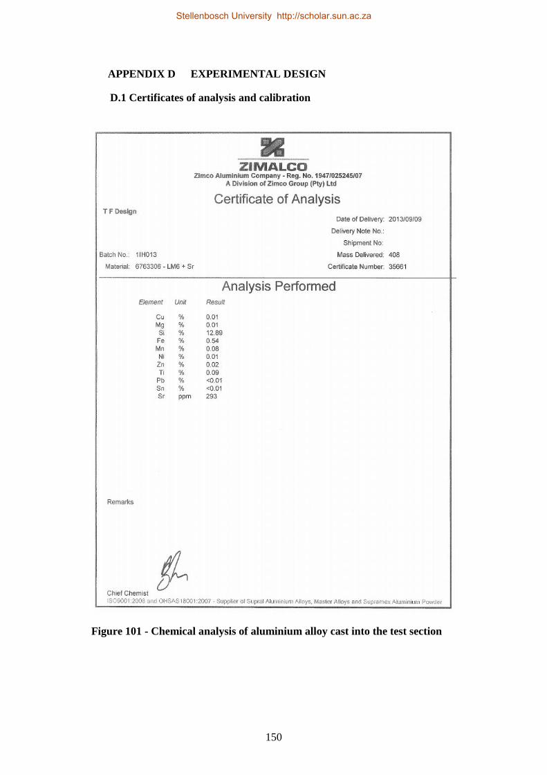
150

APPENDIX D EXPERIMENTAL DESIGN

D.1 Certificates of analysis and calibration

Figure 101 - Chemical analysis of aluminium alloy cast into the test section


151


152

Figure 102 - Certification of compliance for K-type thermocouples

Figure 103 - Calibration certificate - water flow meter


153

D.2 Laminar flow meter design detail

In preliminary design stages of the experimental setup, oil flow rates between 0.1

and 2 kg/s were considered. The flow meter was built from a 6m long 2 inch S10

seamless stainless steel pipe. Using equations 7.28 and 7.29 the design parameters

of the flow meter was evaluated; which is presented in Table 48. The critical

design geometry of the laminar flow meter is presented in Table 49.

Table 48 - Design parameters of the laminar flow meter

Min Max

Mass flow rate 0.10 kg/s 2.00 kg/s

Volumetric flow

rate 1.12E-04 m3/s 2.25E-03 m

3/s

Flow velocity 0.05 m/s 1.04 m/s

Reynolds number 75.69

1513.87

Entrance length 0.20 m 3.97 m

Pressure drop 19.31 Pa 386.15 Pa

Constants

Kinematic

viscosity 3.60E-05 m2/s

Density 890 kg/m³

Length 1 m

Diameter 47.8 mm

Temperature 40 °C

Table 49 - Laminar flow meter critical geometry

Internal diameter 47.8 mm

Entrance length 4 m

Distance between the

pressure taps 1.000 m

Furthermore, the flow meter is insulated using an evacuated annulus around the

central pipe. The reason for this is that the flow meter is highly dependent on the

viscosity of the fluid, which is strongly influenced by the temperature, especially

at lower temperatures. The annulus vacuum is held by a vacuum pump for the

duration of the experiment. The gap between the inner and the outer pipe is held

through star shaped spacers placed throughout the length of the pipe. A drawing

of the flow meter is presented in Figure 104.

The pressure difference between the pressure taps is measured using an

Endress+Hauser Deltabar S PMD75 pressure transducer. The transducer was

calibrated using a Betz micromanometer; the calibration curve is shown in Figure

105. The viscosity of the ISO 100 heat transfer oil was independently tested

according to the ASTM D 445 specification, and the certificate of analysis is

presented in Figure 106. The results of the viscosity test are shown in Figure 107


154

and is presented with a curve fit. The Dynamic viscosity is presented in Figure

108.

Figure 104 - Laminar flow meter drawing

Figure 105 - Calibration curve for the Endress+Hauser Deltabar S PMD75

pressure transducer

y = 189.26x - 749.84

R² = 1

0

500

1000

1500

2000

2500

0 5 10 15 20

Pre

ssu

re P

a

Current, mA

Ch1, mA

Linear (Ch1, mA)


155

Figure 106 - Kinematic viscosity of the ISO 100 heat transfer oil


156

Figure 107 - Kinematic viscosity of ISO 100 oil as a function of temperature

Figure 108 - Dynamic viscosity of ISO100 oil as a function of temperature

The Flow meter was initially calibrated against a SPX In-line hydraulic tester. It

has flow measurement scale of 0 to 200 l/min and an accuracy of 2 % of full scale

(SPX, 2013). The flow meter was connected in series with the hydraulic tester,

and the flow rate was adjusted using the tester’s valve. The resulting calibration

curve is shown in Figure 109. The calibration was done at an oil temperature of

42.5°C.

y = 93 609.113x-1.900

R² = 0.993

0

50

100

150

200

250

300

350

10 20 30 40 50 60 70 80 90

Kin

ema

tic

vis

cosi

ty (

mm

2/s

)

Temperature ( C)

y = 83.312x-1.900

R² = 0.993

0

0.05

0.1

0.15

0.2

0.25

0.3

10 20 30 40 50 60 70 80 90

Dy

na

mic

vis

cosi

ty (

kg

/m.s

)

Temperature ( C)


157

Figure 109 - Calibration curve for the flow meter at 42.5°C

y = 0.00043249x - 0.00171404

R² = 1.00000000

0

0.0001

0.0002

0.0003

0.0004

0.0005

0.0006

0.0007

0.0008

3.5 4.0 4.5 5.0 5.5 6.0

Flo

w r

ate

(m

3/s

)

Pressure transducer readout (mA)


158

APPENDIX E PREDICTION OF THERMAL LOSSES OF THE

TEST SECTION

The heat losses from the surface of the cladding is both convective and radiation.

The outer surface of the classing will be treated as a single smooth polished

stainless steel cylinder. Only these surfaces will be considered because of the

radial nature of the problem. The geometry, emissivity ambient temperature and

surface temperature are presented in 7.4.3.

Table 50 – Geometry, properties and conditions for heat loss estimation

Diameter 0.48 m

Length 1.29 m

Surface area 1.93 m2

Emissivity 0.17

Ambient temperature

(Tamb) 18.00 °C

Surface temperature

(Ts) 49 °C

The natural convective heat transfer coefficient on the surface can be calculated

like that of a vertical plane wall if equation E.1 is met. (Cengel, 2003).

E.1

The Grashof number was evaluated at the film temperature, which is the average

between the ambient and the surface temperatures. The surface temperature of the

cladding was measured at 224 °C and the ambient temperature was measured at

18°C. The properties of air at the film temperature (121 °C) are presented in Table

51:

Table 51 – Air properties at 121°C

2.52E-05 m2/s

β 0.00254

α 3.57E-05 m2/s

k 0.03374 W/m.K

Pr 0.7041

The Grashof number is 1.23x10

10. Substituting the Grashof number into equation

E.1, yields a right-hand side value of 0.121m, satisfying the condition. Thus, the

convection can be taken as that of a vertical plane wall. The Rayleigh number is

8.65x109, yielding a Nusselt number of 1.8x10

2, and this translates to a heat

transfer coefficient, h, of 5.28 W/(m2.K). Using equation E2, the heat transfer

through natural convection is calculated as 1876.25W


159

( ) (E.2)

The radiation heat transfer is calculated using equation E.3 with the properties

listed in Table 50. The radiation heat transfer is calculated as 1586.07W.

(

) (E.3)

This yields total thermal losses of 3462.42W.


160

APPENDIX F HEAT TRANSFER MEASUREMENTS

F.1 Measurement of heat transfer from PCM to Oil

The heat transfer was measured using the 0-20mA output from the flow meter

installation as discussed in Appendix D, and the temperature measurements at the

inlet and outlet of the test section.

To calculate the mass flow rate:

The pressure drop in the laminar flow meter was calculated using the

calibration curve in presented in Figure 105.

The volume flow rate was calculated using equation 7.28.

The mass flow rate was calculated using the properties listed in Table 14

The heat transfer rates was derived using the temperature difference

accross the inlet and the outlet of the test section, and the Cp value listed

in Table 14.

The resulting heat transfer rates for the experiment is presented in Figure 110.

Figure 110 - Heat transfer rates from PCM to oil

Notice that the heat transfer rates begin very high, at about 150 kW, but rapidly

drops down to 50kW, where it slowly decreases with time to below 20kW. This

initial phase of high heat transfer rates corresponds to the sensible discharge of the

PCM as discussed in section 7.5.

0

20

40

60

80

100

120

140

0 1000 2000 3000 4000 5000 6000 7000 8000

Hea

t tr

an

sfer

(k

W)

Time (s)


161

F.2 Measurement of heat transfer from Oil to Water

The water mass flow rates were given directly by the Bürkert SO55 flow meter,

and it was possible to determine the heat transfer using the inlet and outlet

temperatures. The water properties of the IAPWS industrial formulation 1997

were used. The resulting heat transfer rates are presented in Figure 111.

Figure 111 - Heat transfer from oil to water

0

20

40

60

80

100

120

140

0 1000 2000 3000 4000 5000 6000 7000 8000

Hea

t tr

an

sfer

(k

W)

Time (s)


162

APPENDIX G SIMULATION CODE

clear %clear memory

clc %clear screen% Geometrical Constants

%declare global variables

d_pi=0.024; %inner pipe diameter (m)

d_i=0.032; %outer pipe diameter(m)

d_o=0.398; %outer pipe diameter/outer diameter of hexagonal element(m)

L=1.289; %lenth of test section (m)

r_pi=d_pi/2;

r_i=d_i/2;

r_o=d_o/2;

Material properties:

% PCM : AlSi12

T_m=577; %melting point of PCM (degC)

H_f=560000; %heat of fusion (J/kg)

%solis

roh_PCMs=2560; %density around melting point 2700 (kg/m^3)

k_PCMs=160; %thermal conductivity (W/mK)

C_PCMs=2560; %Specific heat capacity of PCM (J/kgK)

%liquid

roh_PCMl=2560; %density around melting point 2700 (kg/m^3)

k_PCMl=160; %thermal conductivity (W/mK)

C_PCMl=1741; %Specific heat capacity of PCM (J/kgK)

%Mildsteel

roh_MS=7854; %density around melting point 2700 (kg/m^3)

k_MS=36.2; %thermal conductivity (W/mK)

C_MS=685; %Specific heat capacity of steel (J/kgK)

%Insert into array

k=[k_MS,k_PCMs,k_PCMl];

roh=[roh_MS,roh_PCMs,roh_PCMl];

Cp=[C_MS,C_PCMs,C_PCMl];

alpha=[(k_MS/(roh_MS*C_MS)),(k_PCMs/(roh_PCMs*C_PCMs)),(k_PCMl/(roh_PCMl*C_PCMl));

%calculation constants

dr=0.001;

dt=0.001;

SimT=3; %hours

%calculate number of increments

nr=(((r_o)-(r_pi))/(dr));

nt=SimT*60*60/dt;

%set up propertie matricies

r=r_pi:dr:r_o; %create a size matrix

T=ones(1,nr); %create temperature matrix

E=ones(1,nr); %create

S=ones(1,nr); %state

Q=ones(1,nr+1); %state

M=ones(1,nr); %Mass

V=ones(1,nr);% create volume matrix

init=ones(1,nr)*630;

T(1,:)=init;

R=zeros(1,nr); %resistance in elements

READOUT=zeros(9,(SimT*3600)/(10));

%READOUTime=10:10:(SimT*3600/10);

READOUT(1,:)=10:10:(SimT*3600);


163

%######################boundary Interfaces#############################

n_i=5;

S(1,1:(n_i-1))=0;

%flags

W=1; %flag to show the solidification thing

TN=1; %flag the time stamp

%initialize properties matricies

for j=1:nr

%Volumes

if j==1

V(1,j)=L*pi*((r(1,j)+dr/2)^2-r(1,j)^2);

else

V(1,j)=L*pi*((r(1,j)+dr/2)^2-(r(1,j)-dr/2)^2);

end

%resistances

if j<n_i

m=1;

R(j)=log((r(j+1))/r(j))/(2*pi()*L*k(m));

elseif j>=n_i

m=2;

R(j)=log((r(j+1))/r(j))/(2*pi()*L*k(m));

end

end

R_conv=1/(2*pi()*(r(1))*L*h_oil);

%enthalpy cutoffs for ALSI12

Tm1=575;

Tm2=577;

H1=0;

H2=Cp(2)*Tm1;

H3=H2+H_f;

A=(H3-H2)/(Tm2-Tm1);

Ti=630;

%mass matrix

for j=1:nr

if j<n_i

m=1;

M(j)=V(j)*roh(m);

elseif j>=n_i

m=3;

M(j)=V(j)*roh(m);

end

end

%energy matrix

for j=1:nr

if j<n_i

m=1;

E(j)=Ti*Cp(m)*M(j);

elseif j>=n_i

if Ti<Tm1

H=Ti*Cp(2);

E(j)=H*M(j);

elseif Ti>Tm2

H=H3+Cp(3)*(Ti-Tm2);

E(j)=H*M(j);

end

end

end

HC=E./M;

for i=1:nt

time=i*dt; %generate time stamp for readout

%heat flow between elemnets

for j=1:nr+1

if j==1


164

if time<40

Q(j)=0;

else

Q(j)=1236*(-7.4465170001*log(time)+91.9651158219);

end

elseif j<nr+1

Q(j)=(T(j)-T(j-1))/R(j-1);

elseif j==nr+1

Q(j)=-3462.42;

end

end

%energy balance on the elements

for j=1:nr

E(j)=E(j)+dt*(Q(j+1)-Q(j));

end

%asign temperatures to nodes

H=E./M;

for j=1:nr

if j<n_i

T(j)=H(j)/Cp(1);

else

if H(j)<H2

T(j)=H(j)/Cp(2);

S(j)=0;

elseif H(j)<H3

T(j)=Tm1+H(j)/A-H2/A;

S(j)=2;

elseif H(j)>=H3

T(j)=Tm2+(H(j)-H3)/Cp(3); % need to be fixed

S(j)=1;

end

end

end

for j=1:nr

if T(j)>Tm1

POS1=r(j);

break

end

end

for j=1:nr

w=nr+1-j;

if T(w)>Tm1

POS2=r(w);

break

end

end

%log the results

if time==(TN*10)

READOUT(2,TN)=T(25);









READOUT(11,TN)=Q(1)/1000;


165

READOUT(12,TN)=Q(nr+1);

READOUT(13,TN)=POS1;

READOUT(14,TN)=POS2;






TN=TN+1

end

end


166

APPENDIX H THERMODYNAMIC ANALYSIS OF THE STEAM

CYCLE

The generating cycle is a regular steam Rankine cycle with the following

properties:


base load operation;




and

Air-cooled condenser (ACC) with a condenser pressure of 0.15 bar with an

air temperature of 30 °C

The steam cycle is represented by the process diagram in Figure 112 below. The

numerical annotation on Figure 112 will be used throughout the analysis.

LP

Turbine

G

HP

Turbine

Open

FW heater

LP FW

Pump

6

HP FW

Pump

10

7

Re-heater

Super heater

Boiler

3

1

8

9

2

Air cooled

condenser

4

5

Figure 112 - Steam Rankine cycle

Assumptions:

Steady state operation

Kinetic and potential energy changes are negligible

Pressure drop through the piping is negligible

The thermal efficiencies of the various components in the Rankine cycle

are shown in Table 52.

Component: Isentropic


167

Efficiency

HP Turbine efficiency: 87%

IP&LP Turbine

efficiency: 87%

Pump 1 efficiency 85%

Pump 2 efficiency 85%

Generator efficiency 95%

Table 52 - Component efficiencies for the steam Rankine cycle

The T-S diagram is presented in Figure 113,

100

200

300

400

500

1 2 3 4 5 6 7

3

1

45

7

6

2

8

9

Entropy (kJ/kg.K)

Tem

per

atu

re (

°C)

Figure 113 - T-S diagram for the Rankine steam cycle

Steam conditions:

State 1: Specified P1 = 140 bar

T1 = 540 °C

h1 = 3434.20 kJ/kg

s1 = 6.53kJ/kgK

ρ1 = 41.10 kg/m3

State 3: Specified P3 = 30 bar

T3 = 540 °C

h3 = 3547.04 kJ/kg

s3 = 7.35 kJ/kgK

ρ3 = 8.147 kg/m3

State5: Saturated liquid of know pressure

(0.15bar)

P5 = 0.15 bar

T5 = 53.97 °C

h5 = 225.94 kJ/kg


168

s5 = 0.755 kJ/kgK

ρ5 = 986.16 kg/m3

State 7: Saturated liquid of a known

pressure (30 bar)

P7 = 30 bar

T7 = 53.97 °C

h7 = 1008.37 kJ/kg s7 = 2.65 kJ/kgK

ρ7 = 821.89 kg/m3

State 9: Saturated steam of a known

pressure (140 bar)

P9 = 140 bar

T9 = 336.67 °C

h9 = 2638.09 kJ/kg s9 = 5.37 kJ/kgK

ρ9 = 87.04 kg/m3

State 2 s2s=s1=6.53 kJ/kgK

using s2s → h2s = 2989.19 kJ/kg

h2=h1-ηt(h1-h2s)

h2=3047.04 kJ/kg

h2 & P2 → T2 = 321.17 °C

P2 = 30 bar

T2 = 321.17 °C

h2 = 3047.04 kJ/kg s2 = 6.63 kJ/kgK

ρ2 = 11.73kg/m3

State 10 State 10 = State 2 P2 = 30 bar

T2 = 321.17 °C

h2 = 3047.04 kJ/kg

s2 = 6.63 kJ/kgK

ρ2 = 11.73kg/m3

State 4 s4s=s3=7.35 kJ/kgK

sg=8.01 kJ/kgK

sf=0.75 kJ/kgK

sfg=7.25 kJ/kgK

x4s = (s4s- [email protected] bar)/sfg=0.909

h4s=hf+ x4shfg=2383.05 kJ/kg

h4=h3-ηt(h3-h4s)= 2534.3 kJ/kg

x4=(h4-hf)/hfg=0.97

s4= sf+ x4sfg = 7.81 kJ/kgK

P4 = 0.15 bar

T4 = 53.97 °C

h4 = 2534.36 kJ/kg

s4 = 7.35 kJ/kgK

ρ4 = 0.0998kg/m3

x4=0.97

State 6 wpump1.in=[v5(P6-P5)]/ηpump1 = 3.56 P6 = 30 bar


169

kJ/kg

h6=h5+ wpump1.in=229.40 kJ/kg

from h6 & P6 : all other properties

T6 = 54.21 °C

h6 = 229.59 kJ/kg

s6 = 2.64 kJ/kgK

ρ6 = 987.34kg/m3

State 8 wpump2.in=[v7(P8-P7)]/ηpump2 =

15.75 kJ/kg

h8=h7+ wpump2.in=1024.11 kJ/kg

from h8 & P8 : all other properties

P8 = 140 bar

T8 = 336.67 °C

h8 = 1024.11 kJ/kg s8 = 5.373 kJ/kgK

ρ8 = 828.43 kg/m3

Steam bleed

flow rate at

condition 10

Let y be the fraction of steam bled

off at the end of the HP turbine.

Then:

( )

Mass flow rate The specified electrical power

output is 100 MW. Taking the

thermal efficiency of the generator

yields that the turbines must

produce 105.3 MW.

By doing a basic energy balance

on the power cycle the mass flow

rate can be calculated.

(( )

( ))

( )(( )

( ))

This yields:

A basic energy balance is presented in Table 53.


170

Mass

flow

(kg/s) (MW)

Turbine 1 93.99 36.39

Turbine 2 68.01 68.87

105.26

Pump 1 68.01 0.24

Pump 2 93.99 1.48

1.72

Boiler 93.99 151.70

Super-heater 93.99 74.83

Re-heater 68.01 34.01

260.54

Thermal

efficiency

0.38

Table 53 - Energy balance of hypothetical power cycle

The boundary conditions and the heat transfer requirements for the steam

generator is presented in Table 54.

Mass

flow

(kg/s)

Enthalpy

change

(kJ/kg) (MW) Tin(°C) Tout(°C) P(bar)

Boiler 93.99 1613.98 151.70 236.85 336.67 140

Super-

heater 93.99 796.11 74.83 336.67 540 140

Re-heater 68.01 500.01 34.01 321.17 540 30


generator


171

APPENDIX I FLOWNEX MODEL

The Flownex model is used to aid in the design of the storage system and the heat

exchange equipment. To obtain boundary conditions for the design of the storage

system and the heat exchangers, the power cycle discussed in section 8.1 and the

boundary conditions developed in appendix H is was used as starting point for the

Flownex model.

Figure 114 - Flownex model of the steam Rankine cycle

The model is shown in Figure 114. The model was built using the designer tool to

fine-tune the component settings to match the conditions of the Rankine cycle

presented in section 8.1. The designer tool uses the Newton-Raphson solution

algorithm to solve a set of non-linear equations. The relation between the

independent variables (such as orifice diameter or turbine efficiency) is set by the

user, and the dependent variables (such as mass flow rate, pressure drop and flow

velocity) in the designer interface. Using a set of boundary conditions, the

Rankine cycle is built up from the inlet of the HP turbine and worked around until

the entire power generating cycle is a closed loop, running both as a steady state

model or a transient state model.

The turbines were modelled with the SimpleTurbine component because the

performance curves of a real turbine could not be obtained, nor does the purpose

of this model merit the level of detail. The simple turbine only takes a constant

isentropic efficiency of the turbine into account. This is in contrast with the

“Turbine” component, which takes the performance curves to calculate the

working point of the turbine depending on shaft speed and steam conditions. The

settings of the high pressure (HP) turbine model are shown in Figure 115. As with

all the components discussed henceforth, the settings and work points of the

components was found using the “Designer tool”.


172

Figure 115 - HP turbine settings

Figure 116 - LP turbine settings

The pumps were simulated by the “Fan or Pump” component. The fan model is

based on a pump chart. Because the feedwater pumps are hypothetical, custom

pumping curves had to be made up. Simple three point pump charts were

constructed around the desired working points, specified by the hand analysis in

appendix H. The pump chart for the low pressure pump is shown in Figure 117

and the HP pump chart is shown in Figure 118.


173

Figure 117 - LP Pump chart

Figure 118 - HP pump chart

Both the open feed water heater and the condenser are modelled using a “Two

phase tank” component. The “two phase tank” is essentially a node with a volume

and a geometry where the level of the tank is determined by the quality (x) of the

two phase fluid in the tank. The height of the outlets to interfacing components

(such as pumps) determines if they receive saturated liquid or saturated steam.

Both were modelled as cylindrical drums with a diameter of 1m, and a length of

3m with flat ends standing vertically. The outlets were set to be at the bottom of

the tank as to only allow saturated water to flow from the node.


174

The flow of turbine bleed steam to the open feed-water heater OFWH is

controlled so that the level of the OFWH is kept at 1.5m (x=0.5). Similarly, the

heat extracted from the condenser is also controlled by changing the heat removed

from the condenser. The condenser pressure is normally controlled by an ejector.

The ejector is simulated by placing a pressure boundary value on the condenser.

The flow rates are controlled by “restrictor with discharge coefficient”

components. The discharge coefficient in all three is set to 1, the number in

parallel is also set to 1 and the cross-sectional diameter was determined by using

the “Designer” tool. The diameter of the restrictor that feed the OFWH was set to

allow 25.98kg/s through (as in the hand calculations). Its diameter is 0.146m.

The restrictors after both pumps have been set up by the “Designer” as to have

the pumps remain at their designed working point. The restrictor after the LP

pump was set using the area function, and was set on 0.001986 m2, and that of the

HP pump was set on 0.065707m on the diameter setting.

Heat input was initially given by the “Custom losses” components. Both of them

had their losses set to zero, but the heat input was added as calculated by hand.

This model runs both in steady state and transient state, and is used as the basis to

add on and design the proper heat exchange and storage equipment.


Thermal energy storage in metallic phase change · PDF fileThermal energy storage in PCMs...

Documents

Transcript of Thermal energy storage in metallic phase change · PDF fileThermal energy storage in PCMs...