Thermal Comfort Conditions Near Highly Glazed Facades: An ...

Thermal Comfort Conditions Near Highly Glazed Facades:

An Experimental and Simulation Study

Mark Bessoudo

A Thesis in the Department of

Building, Civil, and Environmental Engineering

Presented in Partial Fulfillment of the Requirements for the Degree of Master

of Applied Science (Building Engineering) at Concordia University

Montreal, Quebec, Canada

February 2008

© Mark Bessoudo, 2008

1*1 Library and Archives Canada

Published Heritage Branch

395 Wellington Street Ottawa ON K1A0N4 Canada

Bibliotheque et Archives Canada

Direction du Patrimoine de I'edition

395, rue Wellington Ottawa ON K1A0N4 Canada

Your file Votre reference ISBN: 978-0-494-40863-6 Our file Notre reference ISBN: 978-0-494-40863-6

NOTICE: The author has granted a nonexclusive license allowing Library and Archives Canada to reproduce, publish, archive, preserve, conserve, communicate to the public by telecommunication or on the Internet, loan, distribute and sell theses worldwide, for commercial or noncommercial purposes, in microform, paper, electronic and/or any other formats.

AVIS: L'auteur a accorde une licence non exclusive permettant a la Bibliotheque et Archives Canada de reproduire, publier, archiver, sauvegarder, conserver, transmettre au public par telecommunication ou par Plntemet, prefer, distribuer et vendre des theses partout dans le monde, a des fins commerciales ou autres, sur support microforme, papier, electronique et/ou autres formats.

The author retains copyright ownership and moral rights in this thesis. Neither the thesis nor substantial extracts from it may be printed or otherwise reproduced without the author's permission.

L'auteur conserve la propriete du droit d'auteur et des droits moraux qui protege cette these. Ni la these ni des extraits substantiels de celle-ci ne doivent etre imprimes ou autrement reproduits sans son autorisation.

In compliance with the Canadian Privacy Act some supporting forms may have been removed from this thesis.

Conformement a la loi canadienne sur la protection de la vie privee, quelques formulaires secondaires ont ete enleves de cette these.

While these forms may be included in the document page count, their removal does not represent any loss of content from the thesis.

Canada

Bien que ces formulaires aient inclus dans la pagination, il n'y aura aucun contenu manquant.

ABSTRACT

Thermal Comfort Conditions near Glass Facades:

An Experimental and Simulation Study

Mark Bessoudo

There is a current trend of designing new commercial buildings with large

glazed facade areas. Maintaining comfort in the perimeter zones of these

buildings is difficult due to their exposure to solar radiation and cold outdoor air

temperature. Designing these buildings with high-performance fenestration

systems, however, can improve energy performance, provide a high-quality

thermal and visual environment, and reduce thermal loads.

This study presents an experimental and simulation study of thermal

comfort conditions of a perimeter zone office with a glass fagade and solar

shading device. The study investigates the impact of climate, glazing type, and

shading device properties on thermal comfort conditions. The objective of this

study is to determine the facade properties that will provide a comfortable

indoor environment without the need for secondary perimeter heating.

i i i

Experimental measurements were taken in an office equipped with two

different shading devices: Venetian blind and roller shade. The thermal

environment was measured with thermocouples, an indoor climate analyzer, and

thermal comfort meter.

For the simulation study, a one-dimensional transient thermal simulation

model of a typical glazed perimeter zone office and a transient two-node thermal

comfort model were developed. The impact of solar radiation and shading

device properties on thermal comfort was also quantified. Simulation results

were compared with experimental measurements.

The impact of diffuser location for primary heating supply on indoor

airflow and comfort is also investigated using computational fluid dynamics

software and it is shown that good comfort is achieved without the presence of

perimeter heating.

IV

ACKNOWLEDGMENTS

I would like to express my gratitude to my supervisor Dr. A. K. Athienitis for his

continuous encouragement, support, and patience during my graduate studies.

I am also indebted to Dr. A. Tzempelikos for his assistance, support, and advice.

A special thanks to Dr. R. Zmeureanu for his helpful advice.

Many thanks go to my friends and colleagues in the Solar Lab for their

friendship and support.

I would also like to thank my mom, dad, and sister for their unwavering support

and encouragement throughout my studies. I am forever grateful.

Financial support of this work was provided by NSERC through the Solar

Buildings Research Network.

v

To my parents

VI

TABLE OF CONTENTS

LIST OF FIGURES x

LIST OF TABLES xvi

NOMENCLATURE xvii

1 INTRODUCTION 1

1.1 Context 1

1.2 Background 2

1.3 Motivation 4

1.4 Objectives ....5

1.5 Thesis layout 6

2 LITERATURE REVIEW 8

2.1 Thermal comfort 8

2.1.1 The indoor thermal environment 9

2.1.2 Human thermoregulation 12

2.1.3 Prediction of thermal comfort 14

2.1.3.1 Steady-state thermal environments 14

2.1.3.2 Transient thermal environments 17

2.1.4 Conditions for thermal comfort 20

2.1.4.1 The comfort zone 20

2.1.4.2 Local discomfort 22

2.1.4.3 Adaptive approach 26

2.2 Fenestration systems and perimeter zones 28

2.2.1 Windows and glazing 29

2.2.2 Shading devices 32

2.2.3 Mechanical systems 35

2.2.4 Perimeter zones and thermal comfort 38

2.3 Summary 47

vii

3 EXPERIMENTAL STUDY AND RESULTS 48

3.1 Experimental perimeter zone 49

3.2 Data acquisition system, sensors, and measurements 52

3.3 Experimental results 55

3.3.1 Clear winter day 55

3.3.2 Cloudy winter day 59

3.4 Summary 63

4 NUMERICAL SIMULATION STUDY 65

4.1 Description of thermal simulation model 65

4.1.1 Typical meteorological year weather data 66

4.1.2 Solar radiation model 66

4.1.3 Geometry of perimeter zone office 70

4.1.4 Solar radiation transmission through glazing 71

4.1.5 Building thermal simulation model 74

4.1.6 Indoor thermal environment 79

4.2 Comparison of thermal simulation model and measurements 81

4.2.1 Clear winter day: no shading 82

4.2.2 Clear winter day: roller shade 84

4.2.3 Cloudy winter day: no shading 88

4.3 Description of thermal comfort model 90

4.4 Comparison of thermal comfort model with measurements 97

4.5 Parameters and assumptions 99

4.6 Results of simulation study 106

4.6.1 Clear winter day 106

4.6.2 Cloudy winter day 119

4.7 Further investigation using CFD 124

4.7.1 Description of CFD model 125

4.7.2 Results of CFD investigation... 128

5 CONCLUSIONS AND RECOMMENDATIONS 135

5.1 Conclusions 135

5.2 Recommendations for future work 138

REFERENCES 140

APPENDIX A: Perez irradiance model 147

APPENDIX B: Room geometry and view factors 154

APPENDIX C: Building thermal simulation model 166

APPENDIX D: Indoor thermal environment and thermal comfort model 206

IX

LIST OF FIGURES

Figure 2.1: Mean value of angle factors between seated person and horizontal or vertical rectangle (ASHRAE Handbook of Fundamentals, 2005) 11

Figure 2.2: Thermal interaction between the human body and surrounding environment (ASHRAE Handbook of Fundamentals, 2005) 13

Figure 2.3: Relationship between the Predicted Percentage of Dissatisfied (PPD) and Predicted Mean Vote (PMV) (ASHRAE Handbook of Fundamentals, 2005) 17

Figure 2.4: Representation of the concentric skin and core compartments in

the two-node thermal comfort model 19

Figure 2.5: The indoor comfort zone (ASHRAE Standard 55 - 2004) 21

Figure 2.6: Angle factors between a small plane element and surrounding surfaces (ASHRAE Handbook of Fundamentals, 2005) 23

Figure 2.7: Percentage of people dissatisfied for different surfaces (ASHRAE Handbook of Fundamentals, 2005) 24

Figure 2.8: Percentage of people dissatisfied at different air temperatures as a function of mean air velocity (ASHRAE Handbook of Fundamentals, 2005) 26

Figure 2.9: The components of heat transfer through glazing (left) and a simplified view of the components of solar heat gain (Carmody etal.,2004) 31

Figure 2.10: Shortwave (solar) and longwave energy spectrum. Area 1 represents idealized transmittance for low solar heat gain glazing; Area 2 represents idealized transmittance for high solar heat gain glazing (Carmody et al., 2004) 32

Figure 2.11: The perimeter and interior zones of a building (Carmody et al., 2004) 35

Figure 2.12: Cross section of perimeter zone office with typical HVAC configuration: overhead supply air (primary heating) and perimeter baseboard unit beneath glazing (secondary heating)37

Figure 2.13: Sources of thermal discomfort in glazed perimeter zones (Carmody et al., 2004) 38

Figure 2.14: Notation pertinent to calculating the effective radiation area (left) and a chart for determining the projected area factors for a seated person (right) (Rizzo et al., 1991) 43

x

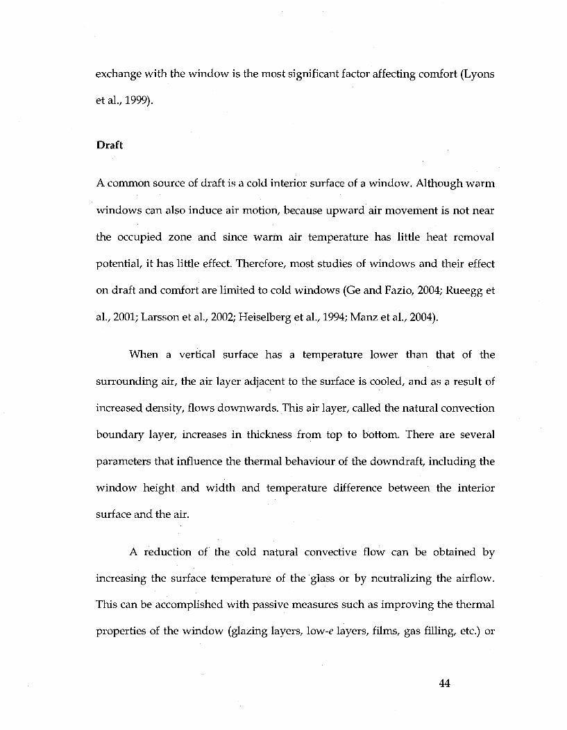
Figure 3.1: The EV Building at Concordia University in Montreal where the experimental measurements were completed (KPMB Architects, 2006). The image on the right shows one of the experimental sections with a dividing curtain 50

Figure 3.2: Schematic of experimental section used for measurements (not to scale) 51

Figure 3.3: Schematic of the six sections of the experimental facade (interior view). The roller shade is used for section 4; the Venetian blinds are used for section 5 51

Figure 3.4: Instruments for measuring indoor environmental parameters: (a) air velocity; (b) shielded air temperature; (c) humidity; (d) plane radiant temperature. (Parsons, 2003) 53

Figure 3.5: Temperature and total incident solar radiation measurements on clear day with no shading 55

Figure 3.6: Temperature and total incident solar radiation measurements on a clear day with roller shade 56

Figure 3.7: Temperature and total incident solar radiation measurements on a clear day with Venetian blind (tilt = 0°) 57



Figure 3.10: Temperature and total incident solar radiation measurements on cloudy day with no shading device 61

Figure 3.11: Temperature and total incident solar radiation measurements on a cloudy day with Venetian blind (tilt = 0°) 61



Figure 4.1: Solar angles for vertical and horizontal surfaces (ASHRAE Handbook of Fundamentals, 2005) 67

Figure 4.2: Direct radiation, ground reflected radiation, and different components of diffuse radiation (Fieber, 2005) 69

Figure 4.3: Graphical representation of view factors for radiation heat transfer calculation (ASHRAE Handbook of Fundamentals, 2005) 71

Figure 4.4: Thermal network diagram of perimeter zone office 75

XI

Figure 4.5: Operative temperature: verification of simulation model with measured values for a clear winter day with no shade 82

Figure 4.6: Room air temperature: verification of simulation model with measured values for a clear winter day with no shade 83

Figure 4.7: Interior glass surface temperature: verification of simulation model with measured values for a clear winter day with no shade 84

Figure 4.8: Operative temperature: verification of simulation model with measured values for a clear winter day with roller shade 85

Figure 4.9: Room air temperature: verification of simulation model with measured values for a clear winter day with roller shade 85

Figure 4.10: Interior glass surface temperature: verification of simulation model with measured values for a clear winter day with roller shade 86

Figure 4.11: Roller shade: verification of simulation model with measured values for a clear winter day with roller shade 87

Figure 4.12: Radiant temperature asymmetry: verification of simulation model and measured values for a clear winter day with roller shade 87

Figure 4.13: Operative temperature: verification of simulation model with measured values for a cloudy winter day with no shade 88

Figure 4.14: Room air temperature: verification of simulation model with measured values for a cloudy winter day with no shade 89

Figure 4.15: Glass temperature: verification of simulation model with measured values for a cloudy winter day with no shade 89

Figure 4.16: Comparison of skin temperature values for thermal comfort simulation model vs. Grivel experimental data 98

Figure 4.17: Comparison of thermal discomfort index for thermal comfort

simulation model vs. Gagge computer model 99

Figure 4.18: Climatic data for representative days used in simulation 100

Figure 4.19: Schematic of typical office used for simulations (not to scale).. 101

Figure 4.20: Effective solar transmittance of glazing as function of incidence angle 102

Figure 4.21: Absorptance of glazing as function of incidence angle 102

Figure 4.22: MRT due to surrounding surfaces only and MRT due to surrounding surfaces and solar radiation with an unshaded double-glazed window on a clear winter day 107

xn

Figure 4.23: Effect of glazing type on interior window surface temperature on a clear winter day 108

Figure 4.24: Effect of glazing type on mean radiant temperature for a clear winter day with no shading 109

Figure 4.25: Effect of glazing type on room air temperature for a clear winter day with no shading.... 109

Figure 4.26: Effect of glazing type on operative temperature for a clear winter day with no shading 110

Figure 4.27: Effect of glazing type on radiant temperature asymmetry for a clear winter day with no shading 110

Figure 4.28: Effect of glazing type on thermal discomfort for a clear winter day with no shading I l l

Figure 4.29: Effect of shade absorptance on shade temperature with glazing 2 (double-glazed, low-e) for a clear winter day 112

Figure 4.30: Effect of shade absorptance on maximum shade temperature for a clear winter day 112

Figure 4.31: Effect of shade absorptance on maximum mean radiant temperature for a clear winter day 113

Figure 4.32: Effect of shade absorptance on maximum room air temperature for a clear winter day 114

Figure 4.33: Effect of shade absorptance on maximum operative temperature for a clear winter day 114

Figure 4.34: Effect of shade absorptance on maximum radiant temperature asymmetry for a clear winter day 115

Figure 4.35: RTA as a function of distance from facade for three different shade absorptances using glazing 1 116



Figure 4.38: Effect of shade absorptance on maximum thermal discomfort for a clear winter day 117

Figure 4.39: Effect of shade absorptance on number of hours per day in discomfort zone for a clear winter day 118

Figure 4.40: Effect of shade absorptance on daily total heating demand for a clear winter day 119

xm

Figure 4.41: Minimum window surface temperature (glazing or shade): Effect of glazing type for a cloudy winter day 120

Figure 4.42: Minimum mean radiant temperature: Effect of glazing type for a cloudy winter day 121

Figure 4.43: Minimum operative temperature: Effect of glazing type for a cloudy winter day 121

Figure 4.44: Minimum thermal discomfort rating: Effect of glazing type for a cloudy winter day 122

Figure 4.45: Daily heating demand: Effect of glazing type for a cloudy winter day 122

Figure 4.46: RTA as a function of distance from facade for glazing 1 with and without shading 123

Figure 4.47: RTA as a function of distance from fagade for glazing 2 with and without shading 123

Figure 4.48: RTA as a function of distance from facade for glazing 3 with and without shading 124

Figure 4.49: Model of perimeter zone office used for Airpak simulation (left); representation of mesh (right) 127

Figure 4.50: Variation in air speed at three different heights with diffuser 0.7 m from window (TSUppiy = 30 °C; vSUppiy = 1.5 m/s) 129

Figure 4.51: Variation in air speed at three different heights with diffuser 1.1 m from window (TSupPiy = 30 °C; vSUppiy = 1.5 m/s) 129

Figure 4.52: Variation in air speed at three different heights with diffuser 1.5 m from window (TSUppiy = 30 °C; vSUppiy = 1.5 m/s) 130

Figure 4.53: Cross sectional contour plot of air speed with diffuser 0.7 m from window 130

Figure 4.54: Cross sectional contour plot of air speed with diffuser 1.1 m from window 131

Figure 4.55: Cross sectional contour plot of air speed with difusser 1.5 m from window 131

Figure 4.56: Cross sectional contour plot of operative temperature with diffuser 0.7 m from window 132



xiv

LIST OF TABLES

Table 4.1: Climatic data for representative days used in simulations 100

Table 4.2: Properties of the three different glazing types used for parametric

analysis (ASHRAE Handbook of Fundamentals, 2005) 103

Table 4.3: Thermal properties of building materials used for simulation 104

Table 4.4: Parameters of indoor environmental conditions and occupant properties used for the thermal comfort simulation 106

xvi

NOMENCLATURE

a horizon brightness coefficient

AD DuBois surface area of body, m2

Acg area of center of glass, m2

Aeg area of edge of glass, m2

Af area of frame, m2

b horizon brightness coefficient

cp specific heat, J / k g K

cp,b specific heat capacity of body, J / k g K

C thermal capacitance

Oes rate of convective heat loss from respiration, W/m 2

DISC index of thermal discomfort

DR draft risk, %

E rate of heat released from body via evaporation, W/m 2

Edif heat transfer by evaporation of moisture through the skin, W/m 2

Emax maximum rate of evaporative heat loss, W / m 2

Esk rate of evaporative heat loss from skin, W / m 2

Eres rate of evaporative heat loss from respiration, W/m 2

Ersw rate of regulatory sweating, W/m 2

sweat rate required for comfort, W/m 2

Fi circumsolar brightening coefficient

F2 horizon brightening coefficient

Fp-i angle factor between person and surface i

Fij angle (view) factor from surface i to surface j

fci clothing area factor

fp projected area factor

he evaporative heat transfer coefficient, W / m 2 k P a

hi interior convective heat transfer coefficient, W/m2 - °C

hn natural convection heat transfer coefficient, W/m2 - °C

xvn

h0 exterior convective heat transfer coefficient, W/m2- °C

hT heat transfer coefficient, radiation, W/m 2 , °C

hc heat transfer coefficient, convection, W/m- °C

im clothing moisture permeability

I total incident solar radiation, W / m 2

lb incident beam solar radiation, W / m 2

Ibh beam horizontal irradiance, W/m 2

Ibn direct normal solar radiation, W/m 2

Ici thermal insulation of clothing, clo

Id total hemispherical diffuse solar radiation, W/m 2

Idg ground reflected diffuse irradiance, W/m 2

Idh sky diffuse horizontal irradiance, W/m 2

k thermal conductivity, W / °C

K heat released from body via conduction, W / m 2

L length, m; thermal load on body, W/m 2

m body mass, kg

M metabolic rate of body, W/m 2

MRT mean radiant temperature

n Julian day number

Nu Nusselt number

Pa partial pressure of water vapour, kPa

PMV Predicted Mean Vote

PPD Predicted Percentage Dissatisfied, %

Psk saturated water vapour pressure on skin surface, kPa

q heat source, W

qSk total rate of heat loss from skin, W / m 2

qres total rate of heat loss through respiration, W / m 2

Q instantaneous heat flow, W

Qcrsk heat transfer from core to skin, W / m 2

R thermal resistance, m 2 °K/W

Ra Rayleigh number

RTA radiant temperature asymmetry, °C

S heat storage in body, W/m 2

Ssk rate of heat storage in skin compartment, W/m 2

Scr rate of heat storage in core compartment, W/m 2

SKBF rate of blood flow from core to skin, kg /hr rn 2

t time, s

tsk,req skin temperature required for comfort, °C

Ta room air temperature, °C

Tb mean body temperature, °C

Tb,c mean body temperature (cold set point), °C

Tb,h mean body temperature (hot set point), °C

Tc comfort temperature, °C

Ti temperature of surface i, °C

Tci temperature of clothing, °C

Tcr temperature of core compartment, °C

Top operative temperature, °C

T0 outdoor air temperature, °C

TSk temperature of skin compartment, °C

TSENS thermal sensation

Tu turbulence, %

U overall heat transfer coefficient, W / m 2 K

Ucg overall heat transfer coefficient for center of glass, W / m 2 K

Ueg overall heat transfer coefficient for edge of glass, W / m 2 K

Uf overall heat transfer coefficient for frame, W / m 2 K

U0 overall heat transfer coefficient of fenestration system, W / m 2 K

v0 outdoor wind speed, m / s

Vsd standard deviation of instantaneous air velocities

V mean velocity, m / s

Vol volume, m3

w skin wettedness

W mechanical work of body, W / m 2

xix

WWR window-to-wall ratio

a s solar altitude

aSk fraction of body mass concentrated in skin compartment

txci,d clothing absorptance for diffuse solar radiation

aci,b clothing absorptance for beam solar radiation

£ emissivity

es emissivity of person

*P surface azimuth angle

P surface tilt angle

o Stefan-Boltzmann constant

p g ground reflectance (albedo)

p density, kg /m 3

9 solar incidence angle

<|> solar azimuth angle

xx

1 INTRODUCTION

1.1 Context

The operation of buildings, including heating, cooling, and lighting, accounts for

roughly 50 per cent of Canada's electricity use and almost 30 per cent of its

energy consumption and greenhouse gas emissions (Ayoub et al., 2000). This

figure could be reduced significantly if buildings were designed to take

advantage of the surrounding climate. An obstacle to implementing energy-

conscious principles into building design, however, is the division of building

systems into different components that are handled separately, often with

conflicting interests. Therefore, in order to attain true energy-efficient buildings,

there is a need for a whole-system view of the building: its structure, subsystems,

and the way they interact with each other, the natural environment, and its

occupants.

Energy-related issues of buildings are only secondary factors; the primary

objective of buildings is to provide shelter, space, and comfort for the people that

live, work, and interact in them. Therefore, the primary objective should not be

neglected in the building design in order to attain energy-efficiency.

1

1.2 Background

It can be said that the "success" of a building depends on whether a comfortable

indoor environment is achieved. Achieving an acceptable indoor environment,

however, is one of the biggest challenges with respect to energy use. There are

several parameters that define the indoor environment including indoor air

quality, visual comfort, and thermal comfort; each has an impact on occupant

health and productivity, and, therefore, the total economic value of the building

(Poirazis, 2005).

Thermal comfort is often listed by occupants as one of the most important

requirements for any building. In surveys of user satisfaction in buildings with

passive solar features, it was found that having the "right temperature" was one

of the most important considerations (Nicol, 1993). Additionally, it was

determined that air freshness was an important requirement. Even the subjective

feeling of air freshness was found to be closely linked to the air temperature.

Therefore, two important requirements of user satisfaction with the indoor

environment are closely related to temperature.

Creating a comfortable indoor environment is also important because

occupants will react to any perceived discomfort by taking actions to restore their

comfort. Sometimes these actions will come with an energy cost; for example,

using a shading device and turning on lights is a costly way to eliminate glare

and overheating due to the presence of solar radiation. Similarly, opening a

2

window in the winter due to overheating is also a costly way to alleviate

discomfort. Therefore, it is important to recognize that a 'low energy' standard

that increases occupant discomfort may be no more sustainable than one that

encourages energy use (Nicol, 2003).

The building envelope is the most critical element of a building and can

influence every other component of the building. A poorly designed envelope

leads to higher energy consumption (for space heating, cooling, and lighting)

and poor comfort conditions in perimeter zones. A well-designed, high-

performance envelope, on the other hand, can improve building energy

performance, provide a higher quality thermal and visual environment, and

reduce peak thermal loads in perimeter zones.

Windows are one of the most significant components of the building

envelope, and therefore of the entire building. Although windows have always

been used as architectural components for providing outdoor view and natural

light, it has only been in recent years that the benefits of windows and their effect

on the satisfaction, health, and productivity of the building occupants have been

recognized (Carmody et al., 2004). This is reflected in the current trend of

designing commercial buildings with glass fagades. In addition to these more

immediate human-related needs, there is also an urgent need for significant

improvements in building energy performance.

3

This growing recognition of the benefits related to the improvement of both

the human-related and energy performance aspects of buildings is evident in the

recent popularity of green building rating systems and certification programs

such as LEED (Leadership in Energy and Environmental Design). These rating

systems require high-quality design in order to deliver superior daylight, views,

comfort, ventilation, and energy performance - all of which are directly related

to fenestration systems (U.S. Green Building Council, 2007). In addition,

sustainable building design requires consideration of passive and active solar

energy systems; good performance of these systems cannot be achieved unless

the integration of solar technologies is considered from the early design stage.

The systems' performance is directly related with the location, form, and

orientation of the building, and, thus, affects the quality of the indoor

environment.

1.3 Motivation

There is a current trend of designing commercial buildings with glass facades.

The reasons for this trend range from providing an expression of transparency

between the client and public to providing conditions that maximize daylighting

and views to aesthetics. In reality, however, these intentions often clash with

occupant behaviour. This is because the building, as a system, is not always

designed with occupant comfort in mind.

4

Although there exist a variety of models that can be used to predict human

thermal comfort, with varying complexity, many are not sufficient to predict

comfort based on the environmental conditions experienced in highly-glazed

perimeter zones. For example, most comfort models used in engineering design

assume steady-state thermal conditions, which is in contrast with the transient

thermal conditions often associated with highly-glazed perimeter zones. In

addition, the most common method to calculate mean radiant temperature

considers interior surface temperatures without considering high-intensity

sources such as solar radiation.

Therefore, there exists an opportunity to develop a thermal comfort model

that takes into account the impact of solar radiation in order to investigate

comfort conditions in highly-glazed perimeter zones. The model will investigate

how the design of facades, including glazing and shading devices, affects

thermal comfort; this knowledge can then be used to determine design

alternatives such as incorporating high-performance glazing and shading in

order to eliminate the need to use secondary perimeter heating.

1.4 Objectives

The objectives of this thesis are to:

5

1. Develop a one-dimensional transient thermal simulation model of a

glazed perimeter zone office environment which incorporates a transient

two-node thermal comfort model

2. Include the effect of solar radiation incident upon a person into the

thermal comfort model

3. Analyze the effect of glazing type and shading properties on the indoor

thermal environment and thermal comfort conditions under various

climatic conditions

4. Determine which facade configurations provide thermal comfort

conditions without the need for a secondary (perimeter) heating system

1.5 Thesis layout

Chapter 2 provides a literature review of thermal comfort, human

thermoregulation, and fenestration systems. Chapter 3 presents the methods and

results of experimental measurements taken in an experimental perimeter zone

office. Chapter 4 presents an overview of the numerical simulation study

detailing the modeling methods used, its verification with experimental

measurements, and results of a parametric analysis using the numerical

simulation model. Chapter 5 provides a summary of the study with conclusions

and recommendations for possible extensions of future work.

6

2 LITERATURE REVIEW

This chapter presents an overview of the major concepts related to thermal

comfort, fenestration systems, and perimeter zones and the interactions between

them. A literature review of the previous experimental and simulation work

completed on these subjects is also presented.

2.1 Thermal comfort

The principle purpose of heating, ventilation, and air-conditioning (HVAC) is to

provide conditions for human thermal comfort (ASHRAE Handbook of

Fundamentals, 2005). ASHRAE Standard 55 (2004) defines thermal comfort as

"that state of mind which expresses satisfaction with the thermal environment".

Although this broad definition has been subject to deep inquiry and

philosophical debate (Cabanac, 1996), it nevertheless emphasizes that the

judgement of comfort is a cognitive process that is influenced by a combination

of physical, psychological, and physiological factors. In general, comfort is

attained when body temperature is held within a narrow range, skin moisture is

low, and the physiological effort of regulation is minimized (ASHRAE

Handbook of Fundamentals, 2005).

8

2.1.1 The indoor thermal environment

From earlier research (Fanger, 1973; Mclntyre, 1980; Gagge et al., 1986), it is

known that thermal comfort is affected by the thermal interaction between the

body and surrounding environment. There are six primary factors that affect this

thermal interaction:

• Air temperature

• Mean radiant temperature (MRT)

• Air speed

• Humidity

• Metabolic rate

• Qothing insulation

The first four factors define the conditions of the surrounding environment

while the latter two represent "personal" variables that can vary between people

exposed to the same environmental conditions.

Mean Radiant Temperature

The mean radiant temperature is defined in ASHRAE Standard 55 (2004) as "the

uniform surface temperature of an imaginary black enclosure in which an occupant

would exchange the same amount of radiant heat as in the actual non-uniform space". It

is an important parameter affecting thermal comfort and also one of the most

difficult parameters to analyze. The MRT (Tmrt) can be calculated with

knowledge of the absolute temperature of the surrounding surfaces (Ti) and the

angle factors between the person and the surrounding surfaces (Fp-i):

9

j 4 = Y r 4 f .

mrf jfj i p-i (2.1)

The angle factors between the person and the surfaces depend on the

posture, position and orientation of the person relative to each surface.

Generally, the angle factors are difficult to determine since the geometry of a

person is complex; however, practical estimates can be made for simplified

analysis with the aid of graphs (Figure 2.1). A simplified algorithm to calculate

these view factors has been developed by Cannistraro et al. (1992) and was found

to give an error of less than 1% when compared to the graphs. The algorithm is

able to calculate the view factors based on the original criteria of posture,

position, and orientation of the person. More complex algorithms to calculate the

view factors of individual body parts to surrounding surfaces have also been

developed, such as the model developed by Zhang et al. (2004) which divides the

surface of the human body into more than five thousand nodes.

A. HOR ?<WTAl »Ex,TANGl F >Oi>« CEI. IM» OR fLOORi

Oft

0 «

ht-t ——— — ;-,

jy^****"*"" ' . ?

/*v~-~**" "' ^ ffls~"" 1 f/s'~~~ 153 M > * " ~ ' 06

££"*"""" »* K-— 0 2

B. VERTICAL RECTANGLE (ABOVE OR BELOW CENTER OF PERSON)

10

Figure 2.1: Mean value of angle factors between seated person and horizontal or vertical rectangle (ASHRAE Handbook of Fundamentals, 2005)

Humidity

Humidity affects the heat loss by evaporation, which is important at high

temperatures and high metabolism, and can have a large impact on the

perception of thermal comfort. In an office space, relative humidity usually

varies between 30% and 60%.

Air Speed

Air speed and turbulence intensity affect the convective heat loss from the body.

A study of air speeds over the whole body in neutral environments found that

air speeds up to 0.25 m / s had no significant effect on thermal acceptability

(ASHRAE Handbook of Fundamentals, 2005).

Clothing Insulation

Clothing provides thermal insulation and its quantity is measured in units of clo,

where 1 clo is equivalent to 0.155 m2K/W. Since people normally adapt their

clothing to suit the climate, typical values of clothing insulation are 0.5 clo in the

summer and 0.9 clo in the winter. Tables of the thermal insulation values of

various clothing ensembles can be found in ASHRAE Handbook of

Fundamentals (2005).

11

2.1.2 Human thermoregulation

In order to quantify how the environment influences thermal comfort, it is

important to first understand the principles of human physiology and

thermoregulation.

The human body produces heat primarily by metabolism, exchanges heat

with the environment via radiation, convection, and conduction, and loses heat

by evaporation of body fluids (Figure 2.2). The metabolic heat generated by a

resting adult is about 100 W. Since this heat is dissipated to the external

environment mainly through the skin, metabolic activity is usually defined in

terms of heat production per unit area of skin. For an average resting person this

is about 58.2 W/m 2 , or 1 met.

The human heat balance equation describes how the body maintains an

internal body temperature close to 37 °C and skin temperature between 33 °C

and 34 °C. The metabolic rate of the body (M) provides energy to the body

needed to do mechanical work (W), with the remainder released as heat (M-W).

Heat is transferred from the body via conduction (K), convection (C), radiation

(R), and evaporation (E). The heat production that is not transferred from the

body provides a rate of heat storage (S). Therefore, the conceptual heat balance

equation is (Parsons, 2003):

M-W = E + R + C + K + S (2.2)

12

Or more specifically:

= (C + R + Esk)+ (Cm + Eres)+ (Ssk + Scr) (2.3)

where:

qsk = total rate of heat loss from skin, W / m 2

qres = total rate of heat loss through respiration, W / m 2

Esk = total rate of evaporative heat loss from skin, W/m 2

Cres = rate of convective heat loss from respiration, W/m 2

Eres - rate of evaporative heat loss from respiration, W/m 2

Ssk = rate of heat storage in skin compartment, W / m 2

So- ~ rate of heat storage in core compartment, W / m 2

SURFACE iH ENVIRONMENT 0)

SURROUNDING

EVAPORATIVE HEAT LOSS (g^)

«eSP IRATrONfC_£ i ^

RADIATION {«) CONVECTION (Ci

SENSIBLE HEAT LOSS FROM SKIN <C*«5

BODY

8KiM{^4 6 }

SWEAT to,.,**

CLOTHING (K^ « , J

EXPOSSD SURFACE

Figure 2.2: Thermal interaction between the human body and surrounding environment (ASHRAE Handbook of Fundamentals, 2005)

The controlled variable for thermoregulation is a combined value of

internal (core) temperatures and skin temperature. The thermoregulatory system

is influenced by internal and external thermal disturbances. Thermoreceptors

13

located in the skin detect external thermal disturbances and enable the

thermoregulatory system to act before the disturbances reach the body core. In

addition to responding to temperature, thermoreceptors also respond to the rate

of temperature change (Hensen, 1990).

The central control system of human thermoregulation, located in the

brain, is the hypothalamus. In order to control various physiological processes of

the body for regulation of body temperature, the hypothalamus is responsible for

autonomic regulation such as heat production (shivering), internal thermal

resistance (control of skin blood flow), external thermal resistance (control of

respiratory dry heat loss), and water secretion and evaporation (sweating and

respiratory evaporative heat loss). These control behaviours are primarily

proportional to deviations from skin and core set point temperatures with some

integral and derivative response aspects involved (ASHRAE Handbook of

Fundamentals, 2005).

2.1.3 Prediction of thermal comfort

2.1.3.1 Steady-state thermal environments

The most significant contribution to research in thermal comfort for practical

application to the built environment was delivered by Fanger in his landmark

publication Thermal Comfort (1973). Fanger outlines the conditions necessary for

thermal comfort and the methods and principles necessary to evaluate thermal

14

environments. These methods and principles are now the most influential and

widely-used throughout the world. The reason for this success is due to the

practical method with which conditions for "average thermal comfort" could be

predicted. Fanger defines three conditions for a person to be in thermal comfort:

1. The body is in heat balance (i.e. no thermal storage; S = 0);

2. The sweat rate is within comfort limits; and

3. The mean skin temperature is within comfort limits.

The objective of Fanger's work was to develop a comfort equation that

required as inputs only the six basic parameters, based on the three conditions

above. The heat balance equation was therefore reduced to:

M-PV = 3.96xl0-8 / c | (rd + 273)4-(Tmrt + 273)4] + / A ( T d - T a )

+3.05[5.73 - 0.007(M - w) - Pa ] + 0.42[(M - w) - 58.12] (2.4)

+0.0173M(5.87 -Pa) + 0.0014M(34 - Ta)

where:

Tcl = 35.7 - 0.0275(M -W)- 0.155Id [(M - W) - 0.007(M -W)-Pa)

-0.42[(M -W)- 58.15] - 0.0173M(5.87 - Pa) - 0.0014 M(34 - TJ] (2.5)

where:

fa = clothing area factor

Tci = temperature of clothing, °C

hc = convective heat transfer coefficient, W/m 2

Ta = room air temperature, °C

Pa = partial pressure of water vapour, kPa

15

An index was created that correlates this heat balance equation with the

mean response of thermal sensation of a large group of people. This index, the

Predicted Mean Vote (PMV), is based on a seven-point scale of thermal

sensation:

+3 hot

+2 warm

+1 slightly warm

0 neutral

- 1 slightly cool

- 2 cool

- 3 cold

The PMV is calculated by:

PMV = [0.303 exp(-0.036M) + 0.028]L (2.6)

where L is the thermal load on the body, defined as "the difference between internal

heat production and heat loss to the actual environment for a person hypothetically kept

at comfort values of the mean skin temperature and sweat secretion at the actual activity

level" (ASHRAE Handbook of Fundamentals, 2005). It is essentially the difference

between the left and right sides of the heat balance equation. In comfort

conditions the thermal load will be zero (i.e. PMV = 0). Therefore, for deviations

from comfort condition, the thermal sensation experienced will be a function of

the thermal load and activity level.

With the PMV value known, it is possible to estimate the percentage of

people who would be dissatisfied with the given environmental conditions. This

16

index, called Predicted Percentage Dissatisfied (PPD), is a function of the PMV

index:

PPD = 100 - 95exp[-(0.03353PMV4 + 0.2179PMV2)] (2.7)

An acceptable thermal environment for general comfort is within the

range of -0.5 to +0.5, corresponding to a PPD < 10%. It can be seen from Figure

2.3 that even at thermal neutrality (L = 0, PMV = 0), 5% of the people are

expected to be dissatisfied. The PMV-PPD model is widely used for practical

application and is accepted for design and field assessment of comfort

conditions.

PREDICTED MEAN VOTE

Figure 2.3: Relationship between the Predicted Percentage of Dissatisfied (PPD) and Predicted Mean Vote (PMV) (ASHRAE Handbook of Fundamentals, 2005)

2.1.3.2 Transient thermal environments

Because of the thermal interaction between the HVAC system, climate, building

mass, and occupancy, pure steady-state conditions rarely exist in practice. This is

even more evident in the perimeter zones of buildings where interaction between

17

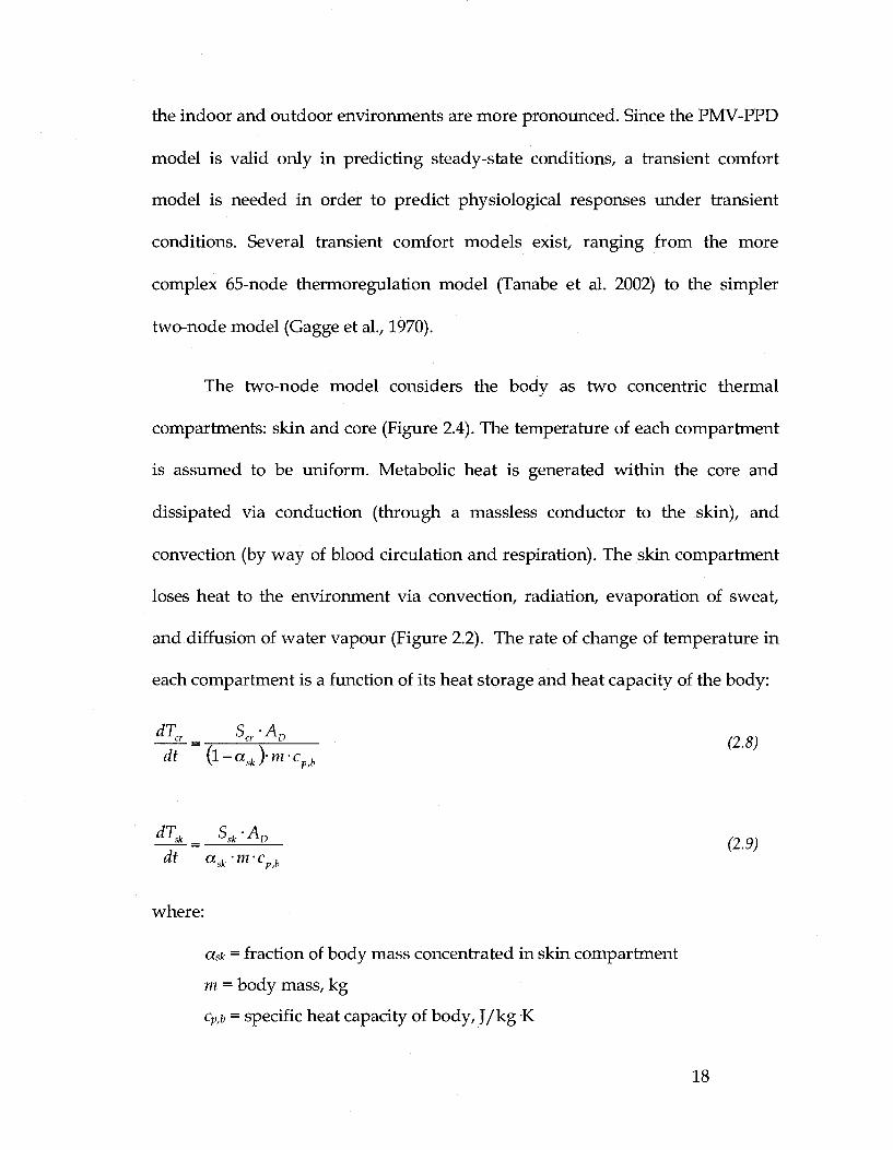
the indoor and outdoor environments are more pronounced. Since the PMV-PPD

model is valid only in predicting steady-state conditions, a transient comfort

model is needed in order to predict physiological responses under transient

conditions. Several transient comfort models exist, ranging from the more

complex 65-node thermoregulation model (Tanabe et al. 2002) to the simpler

two-node model (Gagge et al., 1970).

The two-node model considers the body as two concentric thermal

compartments: skin and core (Figure 2.4). The temperature of each compartment

is assumed to be uniform. Metabolic heat is generated within the core and

dissipated via conduction (through a massless conductor to the skin), and

convection (by way of blood circulation and respiration). The skin compartment

loses heat to the environment via convection, radiation, evaporation of sweat,

and diffusion of water vapour (Figure 2.2). The rate of change of temperature in

each compartment is a function of its heat storage and heat capacity of the body:

£LL.= — ^ A R (2.8) & \X-ask}m-c

P,b

"hk _ ^sk ' ^P ft g\ dt ccsk-m-cp/h

where:

aSk = fraction of body mass concentrated in skin compartment

m = body mass, kg

cp,b = specific heat capacity of body, J/ kg K

18

AD = DuBois surface area, m2

Tcr = temperature of core compartment, °C

Tsk = temperature of skin compartment, °C

t - time, s

Figure 2.4: Representation of the concentric skin and core compartments in the two-node thermal comfort model

The heat storage in each compartment can be expressed as:

Scr=M-W-(Cres -Eres)-Qcrsk (2.10)

Ssk=Qcrsk-(C + R + Esk) (2.11)

where Qcrsk [W/m2] is the heat transfer from the core to the skin by convection

through blood circulation and by conduction through the body tissue.

Thermoregulatory control processes (rate of blood flow, sweating and

shivering) are governed by temperature signals from the skin and core. These

signals are assumed to be proportional to the difference between actual

temperature and corresponding set-point temperature for neutral condition

(Zmeureanu and Doramajian, 1992).

19

By determining the values of skin temperature, core temperature, and skin

wettedness, the two-node model uses empirical expressions to predict thermal

sensation (TSENS) and thermal discomfort (DISC). Both of these indices are

based on 11-point scales, with positive values representing the warm side of the

neutral sensation and the negative values representing the cold side. TSENS is

based on the same scale as the PMV index, but with extra values of +4 and ±5

indicating very hot/ cold and intolerably hot/cold, respectively.

2.1.4 Conditions for thermal comfort

2.1.4.1 The comfort zone

Since neither MRT nor dry-bulb temperature alone are good thermal comfort

indicators, Fanger (1967) suggested using the operative temperature (Top) as an

indicator. The operative temperature is defined as "the uniform temperature of an

imaginary black enclosure in which an occupant would exchange the same amount of

heat by radiation plus convection as in the actual non-uniform environment" and can

be calculated as the average of the MRT and air temperature weighted by their

respective heat transfer coefficients:

T „ , - ^ i (2.12) hr+hc

ASHRAE Standard 55 (2004) specifies conditions (operative temperature

and humidity) where 80% of sedentary or slightly active people will find the

20

thermal environment acceptable (PPD < 20%) (Figure 2.5). Since people typically

change their clothing for different seasons, ASHRAE Standard 55 (2004) specifies

summer and winter comfort zones differentiating between clothing insulation

levels of 0.5 and 0.9 clo, respectively. Within the comfort zones, a typical person

wearing the prescribed clothing insulation levels would have a thermal sensation

at or near neutrality (-0.5 < PMV < +0.5). The comfort zones are also only valid

for primarily sedentary activity (1.0 met < M < 1.3 met) in low velocity

environments (v < 0.2m/s).

18 18 20 22 24 26 28 30 32

OPERATIVE TEMPERATURE, "C

Figure 2.5: The indoor comfort zone (ASHRAE Standard 55 - 2004)

It should be noted that although ASHRAE Standard 55 (2004) states that

environmental conditions should be kept within the comfort zone, it also allows

for the operative temperature to temporarily deviate from the limits of the

21

comfort zone. Temperature drifts or ramps are allowed, for example, given that

the operative temperature does not change more than 1.1 °C during a 15-minute

period or 2.2 °C during a one-hour period. Based on these criteria, Zmeureanu

and Doramajian (1992) were able to demonstrate that energy savings could be

obtained in office buildings in the summer if the indoor air temperature was

allowed to drift in the afternoon, exceeding the upper limit of the comfort zone.

2.1.4.2 Local discomfort

Although a person may feel thermally neutral as a whole, there may be instances

when they still feel uncomfortable due to one or more body parts being too

warm or too cold. These non-uniformities may be due to a cold window, a hot

surface, a draft, or a temporal variation of these. The comfort zones of ASHRAE

Standard 55 (2004) specify a thermal acceptability level of 90% if the environment

is thermally uniform, but since the Standard's objective is to specify conditions

for 80% acceptability, it is permitted to decrease acceptability by 10% due to local

non-uniformities.

Radiant Temperature Asymmetry

A non-uniform thermal environment will give rise to radiant temperature

asymmetry (RTA). It is defined as the difference between the plane radiant

temperatures of two opposite sides of a small plane element, where the plane

radiant temperature quantifies the thermal radiation in one direction. The angle

22

factors between a small plane element and surrounding surfaces can be

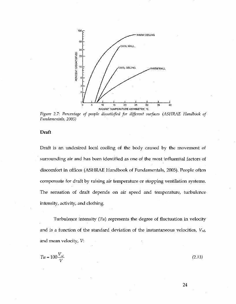
determined from Figure 2.6. ASHRAE Standard 55 (2004) recommends that RTA

due to a warm wall should not exceed 23 °C and 10 °C for a cool wall. Figure 2.7

shows the predicted percentage of dissatisfied occupants as a function of RTA

due to a cool or warm wall or ceiling.

Figure 2.6: Angle factors between a small plane element and surrounding surfaces (ASHRAE Handbook of Fundamentals, 2005)

23

WARM CEILING

WARM WALL

0 5 10 15 20 25 30 3S 40 RADIANT TEMPERATURE ASYMMETRY. °C

Figure 2.7: Percentage of people dissatisfied for different surfaces (ASHRAE Handbook of Fundamentals, 2005)

Draft

Draft is an undesired local cooling of the body caused by the movement of

surrounding air and has been identified as one of the most influential factors of

discomfort in offices (ASHRAE Handbook of Fundamentals, 2005). People often

compensate for draft by raising air temperature or stopping ventilation systems.

The sensation of draft depends on air speed and temperature, turbulence

intensity, activity, and clothing.

Turbulence intensity (Tu) represents the degree of fluctuation in velocity

and is a function of the standard deviation of the instantaneous velocities, Vsd,

and mean velocity, V:

Tu = 1 0 0 ^ -V

(2.13)

24

Air speed and turbulence intensity affect the convective heat loss from the

body. A study of air speeds over the whole body in neutral environments found

that air speeds up to 0.25 m / s had no significant effect on thermal acceptability.

However, air temperature has a significant influence on the percentage of

dissatisfied due to mean air speed (Figure 2.8) (ASHRAE Handbook of

Fundamentals, 2005).

It has been found that there is a much higher percentage of people

dissatisfied for situations with fluctuating velocity than of constant velocity

(Huizenga et al., 2006). Fanger et al. (1988) investigated the effect of turbulence

intensity on sensation of draft and developed an equation to predict the

percentage of people dissatisfied due to draft risk (DR):

DR = (34 - Ta ){V - 0.05)062 (0.37V • Tu + 3.14) (2.14)

ASHRAE Standard 55 (2004) states that the maximum draft risk for

maintaining comfort is 20%.

25

80

80

40

O

<£

< s» w

3 8 I 6 o tc 4 »

2

1 0 Q.t 0,2 0:3 0.4 0.5

MEAN AtR VELOCITY, mis

Figure 2.8: Percentage of people dissatisfied at different air temperatures as a function of mean air velocity (ASHRAE Handbook of Fundamentals, 2005)

2.1.4.3 Adaptive approach

The adaptive approach to thermal comfort is not related to thermoregulatory

modeling. Rather, it is based on the observation that there is a range of actions, or

"adaptive opportunities" that a person can perform in order to achieve thermal

comfort. Adaptive opportunities, which include the ability of an occupant to

open a window, draw a blind, use a fan, or change clothing, increase the

"forgiveness" of the building (i.e. occupants will overlook shortcomings in the

thermal environment more readily) and will therefore have a beneficial effect on

occupant's perception of comfort. The adaptive approach is best expressed with

the adaptive principle: "if a change occurs such as to produce discomfort, people react

in ways which tend to restore their comfort" (Nicol and Humphreys, 2002).

Nicol and Humphreys also state that the adaptive approach is dependent

on many factors (climate, HVAC systems, and time) and context dependent (i.e.

26

solar shading on an appropriate facade). Adaptive thermal comfort is a function

of the possibilities for change as well as the actual temperatures achieved. For

example, in situations where there are no possibilities for changing clothing or

air movement, the comfort zone may have a range as narrow as ±2 °C, whereas

situations where adaptive opportunities are available and appropriate, the

comfort zone may be considerably wider.

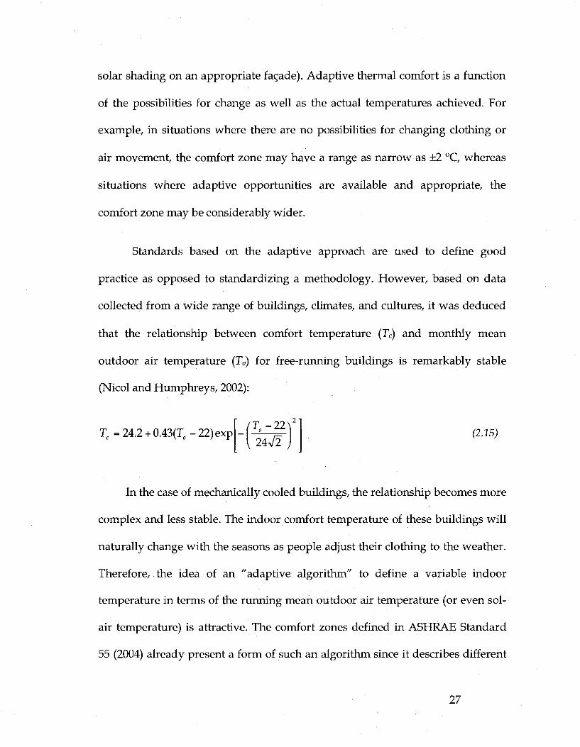
Standards based on the adaptive approach are used to define good

practice as opposed to standardizing a methodology. However, based on data

collected from a wide range of buildings, climates, and cultures, it was deduced

that the relationship between comfort temperature (Tc) and monthly mean

outdoor air temperature (T0) for free-running buildings is remarkably stable

(Nicol and Humphreys, 2002):

Tc =24.2 + 0.43(T0-22)exp 'T0-22\2

24V2 j (2.25;

In the case of mechanically cooled buildings, the relationship becomes more

complex and less stable. The indoor comfort temperature of these buildings will

naturally change with the seasons as people adjust their clothing to the weather.

Therefore, the idea of an "adaptive algorithm" to define a variable indoor

temperature in terms of the running mean outdoor air temperature (or even sol-

air temperature) is attractive. The comfort zones defined in ASHRAE Standard

55 (2004) already present a form of such an algorithm since it describes different

27

indoor ranges of operative temperatures and simply named "winter" and

"summer". These seasonal temperature ranges are based on crude assumptions

about the seasonal change in clothing insulation and metabolic rate. The adaptive

algorithm, on the other hand, does not rely on these vague descriptions. Rather,

it relates the comfort temperature directly to the running mean of the outdoor air

temperature. It is even suggested that such a method does not increase occupant

discomfort, yet significantly reduces energy consumption of the cooling system

compared to a method using a constant indoor set point.

2.2 Fenestration systems and perimeter zones

Fenestration is a term that refers to windows, skylights, and door systems within

a building. Fenestration system components of windows include glazing,

framing, and shading devices (interior, exterior, integral). The principle energy

concern of fenestration systems is their ability to control heat gains losses. They

affect building energy use through four basic mechanisms: heat transfer

(conduction, convection, radiation), solar heat gain, air leakage, and daylighting.

Therefore, fenestration systems play a significant role in the heating, cooling, and

lighting loads of perimeter zones. The recognition of the benefits that can be

attained by providing occupants with better access to daylight, views, and fresh

air is leading to buildings that are thinner in profile with more perimeter and

fewer core zones (Carmody et al., 2004).

28

2.2.1 Windows and glazing

The primary energy concern of windows is their ability to control heat loss. Heat

transfer through window systems is an interaction of all heat transfer

mechanisms: conduction, convection, and radiation. The standard way to

quantify this heat flow is with the U-value - an expression of the total heat

transfer coefficient of the window system. For a single pane of glass, the U-value

is:

U (2.26) l/hl+l/h0+l/k

where hi and h0 are the interior and exterior heat transfer coefficients (combined

convection and radiation), respectively, / is the thickness of the glass, and k is the

thermal conductivity of the glass.

The overall U-value of a fenestration system (U0) can be determined

knowing the separate heat transfer contributions of the center-of-glass, edge-of-

glass, and frame (subscripts eg, eg, and f) in the absence of solar radiation. The

total U-value thus becomes a weighted average of these contributions (ASHRAE

Handbook of Fundamentals, 2005):

u..u«A*+u-A< + u'A> (217)

where A0 is the overall area of the fenestration system.

29

Another major energy-related characteristic of windows is their ability to

control solar heat gain. When direct and diffuse solar radiation coming from the

sun and sky is incident on a window, some is transmitted to the interior and

some is absorbed in the glazing and readmitted to the interior (Figure 2.9). The

solar heat gain coefficient (SHGC) is the fraction of incident solar radiation that

actually gets transmitted to the interior as heat gain. It is a dimensionless number

from 0 to 1.

Therefore, the basic equation for the instantaneous energy flow through a

fenestration system, Q, is (ASHRAE Handbook of Fundamentals, 2005):

Q = U-A-{T0-Ti)+SHGC-A-I (2.18)

where:

Q = instantaneous energy flow, W

U = overall heat transfer coefficient, W/m2K

T0 = exterior air temperature, °C

Ti = interior air temperature, °C

I = incident solar radiation, W / m 2

30

II

#

Outdoor

v"*"*'

0

Double-glazed window

Indoor Conduction

Convection

Thermal radiation

w f f *

Double-glazed wWow

Solar trartsmrttarw

Reflected radiation

Outdoor

H»— Absorbed radiation

Indoor

InwawMfowing component of absorbed radiation

Figure 2.9: The components of heat transfer through glazing (left) and a simplified view of the components of solar heat gain (Carmody et ah, 2004)

The glazing component of fenestration systems can be comprised of single

or multiple layers, usually glass. The glass can be clear, tinted, and / or have

coatings. Spectrally selective coatings, those that select specific portions of the

energy spectrum to reflect or transmit, can be applied to windows and be

designed to optimize energy flows for passive solar heating and daylighting

(Figure 2.10). The emittance of glazing is also an important component for the

overall heat transfer of a window. Reducing the emittance of a window can

greatly improve its thermal performance. The most common type of coating is

one that exhibits low-emissivity (low-e) over the longwavelength portion of the

solar spectrum.

There are two types of low-e coatings: low-solar-gain coatings and high-

solar gain coatings. The low-solar-gain coatings are able to reduce solar heat gain

by transmitting visible light but reflecting the infrared portion of the solar

31

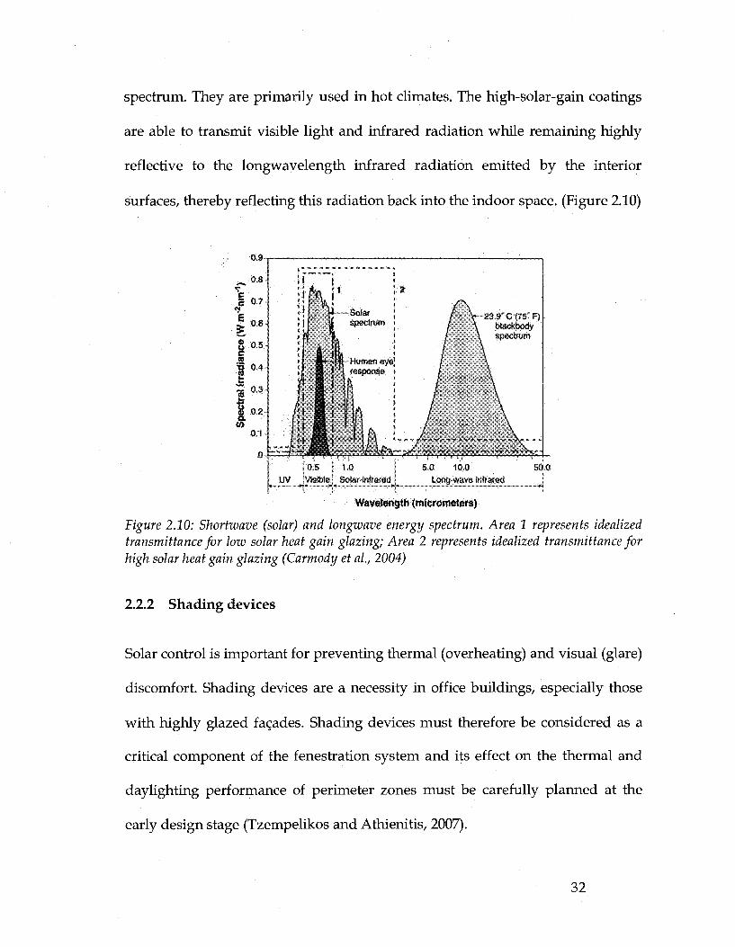
spectrum. They are primarily used in hot climates. The high-solar-gain coatings

are able to transmit visible light and infrared radiation while remaining highly

reflective to the longwavelength infrared radiation emitted by the interior

surfaces, thereby reflecting this radiation back into the indoor space. (Figure 2.10)

o.s ; 1.0 UV ^yisibiej^ Solar-infrared

5.0 10.0 Long-wave infrared

50.0

Wavelength (micrometers)

Figure 2.10: Shortwave (solar) and longwave energy spectrum. Area 1 represents idealized transmittance for low solar heat gain glazing; Area 2 represents idealized transmittance for high solar heat gain glazing (Carmody et ah, 2004)

2.2.2 Shading devices

Solar control is important for preventing thermal (overheating) and visual (glare)

discomfort. Shading devices are a necessity in office buildings, especially those

with highly glazed facades. Shading devices must therefore be considered as a

critical component of the fenestration system and its effect on the thermal and

daylighting performance of perimeter zones must be carefully planned at the

early design stage (Tzempelikos and Athienitis, 2007).

32

Shading devices can either be exterior to, interior to, or within the glazing

system. Types include Venetian blinds, roller shades, draperies, side fins,

awnings, and overhangs. Exterior shading devices reduce solar heat gain more

effectively than interior devices since a significant portion of solar radiation is

rejected to the outdoor environment. However, exterior shading devices are not

as versatile as interior shading devices since they must be robust enough to

withstand the effects of the exterior environmental conditions.

Several studies have shown how the energy performance of a fenestration

system is greatly affected by the presence of a shading device (Tzempelikos et al.,

2007; Tzempelikos and Athienitis, 2007; Shahid and Naylor, 2005; Collins et al.,

2002).

The thermal resistance of a window system with automated intermediate

Venetian blinds was measured experimentally by Tzempelikos and Athienitis

(2003). The thermal resistance of the window system varied in the range of 0.52 -

0.78 m2K/W, depending on the blind tilt angle, |3:

, N 0.068(i3-90°)2 + (-4)(/8-90°) + 600 R(B = X- 1—^-JV / (2.19)

v ; 1000

Although the coefficients in this equation will change for different slat

widths, slat distance, blind properties, and gap width, it was concluded that for

this type of window system, the thermal resistance of the window is determined

33

by the blind tilt angle; the temperature difference between inside and outside

had a small impact.

In another study examining the effects of louver angle (cp) of an internal

Venetian blind on the thermal performance of a window, Shahid and Naylor

(2005) demonstrated that the presence of a Venetian blind significantly improves

the energy performance of a single- and double-glazed window during ASHRAE

summer design conditions. It achieves this by reducing the overall heat transfer

rate through the window thereby reducing the thermal radiation from the

interior glazing. It was determined that the blind had the greatest impact on

energy performance of a window when the louvers were fully closed (cp = 90°),

reducing the U-value of a single-glazed window by 22% when compared to a

window with no blind. With the blind's louvers at a horizontal position (cp = 0°),

the U-value could be reduced by 11%. Similarly, for a double-glazed window,

the blinds in a fully closed position and horizontal position could reduce the

window U-value by 18% and 10%, respectively. In addition, the study also

quantified the effect that the blind has in shielding a nearby occupant from

radiative heat flux. It was found that for a single-glazed window, the blind

reduced the radiative heat transfer by 15% when cp = 0° and 42% when cp = 90°.

For a double-glazed window, the blind reduced the radiative heat transfer by

12% and 37% for louver angles of 0° and 90°, respectively.

34

2.2.3 Mechanical systems

All commercial buildings are divided into thermal zones (Figure 2.11). These

zones represent areas of the building that are served by different HVAC systems.

A mechanical system zone may operate like a separate building in that it receives

heating, cooling, and ventilation from either its own packaged unit or a central

system as needed. A building is divided into zones because different spaces have

different temperature and outdoor air requirements and therefore need separate

control. Zones are also divided based on the orientation of perimeter zone's

fagade. For example, a north-facing perimeter zone may require heat in the

winter while a south-facing perimeter zone within the same building may not

due to passive solar gains. Perimeter zones, especially those with fenestration

systems, are subject to the greatest fluctuation in thermal conditions due to its

direct exposure to outdoor environmental conditions.

ir rJSk

Perirrwswr zones

Interior zones

-j^3ft

Figure 2.11: The perimeter and interior zones of a building (Carmody et ah, 2004)

35

Traditionally, windows have affected the mechanical design of buildings

by increasing the size of mechanical equipment needed for heating and cooling.

While a majority of the buildings conditioning needs are delivered through

forced-air HVAC systems, additional radiant and connective perimeter

baseboard heating is often required near windows in order to mitigate

downdraft (Figure 2.12).

With high-performance windows, heat loss and gain though the window

is reduced significantly, lowering the peak heating and cooling loads, thereby

reducing the size of the mechanical systems. Thus, they play an important role in

reducing building energy consumption; a better understanding of how high-

performance windows affect occupant comfort could accrue even greater

savings. For example, as windows become more insulating, baseboard heaters

can be replaced with slot diffusers delivering heated air from above the window.

With highly insulating windows, a perimeter heating system may not be needed

at all. A recent study found that when high-performance windows are used in

houses, perimeter heating systems could be eliminated and energy savings of

10% - 15% could result from installing a simpler, less expensive duct system

(Hawthorne and Reilly, 2000).

In another case study of facade and envelope design options for a large

commercial building in Montreal, Tzempelikos et al. (2007) investigated the

effect of window-to-wall ratio (WWR) and glazing type on thermal performance

of a perimeter zone office (4m x 4m x 4.25m). After studying the thermal

36

performance of three glazing types, it was determined that a low-e double

glazing would need perimeter heating while a more insulated glazing

(R=0.67m2K/W) would not (WWR = 0.6).

A study by Tzempelikos and Athienitis (2007) showed the benefits of

integrated daylighting, shading, and electric lighting control. It was

demonstrated that optimum energy performance is only achieved if daylighting

benefits due to reduced electric lighting operation exceed the increase in energy

demand due to increased solar gains.

(Primary) Swpply air Return air

Tra ( 4^> -?<fc-

i/ {Secondary} Perimeter heating

Figure 2.12: Cross section of perimeter zone office with typical HVAC configuration: overhead supply air (primary heating) and perimeter baseboard unit beneath glazing (secondary heating)

37

2.2.4 Perimeter zones and thermal comfort

The presence of fenestration systems adds complexity to the problem of human

thermal comfort since fenestration components have different optical and

thermal properties. For perimeter zones, it is important to take into account the

effect that solar radiation has on the thermal environment since HVAC systems

rarely achieve perfect control and, as a result, solar gain often raises the operative

temperature of the perimeter zone.

Fenestration systems influence thermal comfort in three ways (Figure 2.13):

1. longwave radiation exchange between body and warm/cold interior

window surface;

2. transmitted solar radiation; and

3. convective drafts induced by difference between interior window surface

temperature and adjacent air temperature.

Figure 2.13: Sources of thermal discomfort in glazed perimeter zones (Carmody et at, 2004)

38

Thermal comfort is affected indirectly by the solar radiation absorbed in

the fenestration system and interior surfaces, and directly by the transmitted

solar radiation absorbed by the occupant.

Solar transmittance is the dominant factor with respect to the effect a

particular glazing system will have on comfort. Simulations have shown that a

double 3 mm low-e glass with solar transmittance of 0.53 can reduce discomfort

by more than 50% when compared with a single 3 mm clear glass and solar

transmittance of 0.83 (Lyons et al., 1999).

Carmody et al. (2004) carried out an extensive study into the effect of

various facade designs of large commercial buildings on the indoor

environmental and energy performance of perimeter zones. The performance of

a typical perimeter zone office was analyzed (energy use, peak loads,

daylighting, glare, thermal comfort) using different parameters (shading device,

glazing properties, lighting control) for different climates. It was determined that

for south-facing perimeter zones with large window area (WWR = 0.6), interior

shades improve thermal comfort for all window types except the double-glazed

reflective window. For poor glazing, such as a double-glazed, clear window,

overhangs and interior shades provided the biggest positive impact on comfort.

For east- and west-facing perimeter zones with a large window area (WWR =

0.6), interior shades improve comfort, however, only the interior shaded triple-

glazed, low-e window attained the criteria of PPD < 20%. Overall, it was found

that shading is recommended for large window areas, for all window types.

39

Interior shades result in a significant improvement in energy use; even high-rise

obstructions do not offset the need for shading.

A methodology to quantify the impact of fenestration systems on thermal

comfort was developed by Chapman et 'al. (2003) using the radiant intensity

method. This method considers discrete directions and nodes and calculates the

radiant intensity at each point and direction within an enclosure. The enclosure

space is divided into a three-dimensional space of finite control volumes. Four

different cases were analyzed for rooms with and without fenestration systems

and with and without a heating system. Comfort (defined as the operative

temperature corresponding to a PPD of 10%) was quantified as a percentage of

total floor space by plotting the PMV distribution across the room as contour

plots. It was determined through this analysis that "whole-room" heating or

cooling systems, such as forced air systems, do not impact the thermal comfort

distribution created by the fenestration system. The "penetration depth" was

introduced as a new metric for quantifying comfort, defined as the distance from

the fenestration into the room, beyond which thermally comfortable conditions

exist.

A study for the potential of electrochromic (EC) vacuum glazing (VG) to

improve thermal comfort was completed by Fang et al. (2006). Using a finite

volume model to analyze the heat transfer through an EC VG for ASTM standard

winter boundary conditions, it was shown that when the EC layer faced the

interior, glazing surface temperatures would be too high for occupant comfort;

40

therefore, it was recommended that the EC layer be facing the outdoor

environment. With an indoor set-point temperature of 20°C and outdoor

temperature of -20°C, it was shown that for incident solar radiation from 0 to

1000 W / m 2 interior surface temperature of the window increased from 13.4°C to

56.0°C. At an incident solar radiation level of 200 W/m 2 , the interior window

surface begins to transfer heat to the interior. Based on these results, the authors

concluded that their results suggest that EC VGs are comparable to a good triple-

glazed window in terms of thermal performance.

Another emerging technology used to improve comfort in perimeter

zones is electrically heated windows. When an electrical current is switched to a

selective layer on a window pane, the entire glazing can be heated. This presents

a unique opportunity for comfort conditioning in cold climates. When properly

located, electrically heated zones of a window can avoid downdraft and

asymmetric radiation caused by cold interior surfaces. Laboratory measurements

conducted by Kurnitski et al. (2003) show that electrically heated windows are an

efficient way for thermal conditioning when heated zones are properly

dimensioned and proper surface temperatures are used.

Mean Radiant Temperature

The method for calculating MRT as discussed in the previous section is valid

when a person is exposed only to low-temperature surfaces emitting longwave

radiation. If a person is situated near a window, however, the MRT is also

41

affected by the solar radiation hitting the body. Therefore, the previous equation

is inadequate to accurately describe the MRT for a person situated near a

window. A generalized algorithm to calculate the MRT of a person exposed to

solar radiation has been developed by La Gennusa et al. (2005):

N -I / M \

*r ~ 2J p-i ' + airr,d 2J P~j d>) + ain,b)v'-\ £.0

\ r i-i

(2.20)

where:

ss = emissivity of the person

cxirr,d = absorptivity of person for diffuse solar radiation

ctinvb = absorptivity of person for beam solar radiation

Fp.j = view factor of the person to any non-opaque element of the

building envelope

fp = projected area factor

This equation takes into account the effect of three separate components

on the MRT: low-temperature surfaces, absorbed diffuse solar radiation, and

absorbed direct beam solar radiation. The amount of direct beam solar radiation

striking the person is dependent on the solar geometry relative to the person,

since the projection of the sun onto the person, or projected area factor, changes

with the sun's altitude, azimuth, and person's orientation (Figure 2.14). Although

the projected area factor for seated or standing persons can be determined

manually from graphs (Figure 2.14), an algorithm to calculate it explicitly

(discussed in detail in Chapter 4) was developed by Rizzo et al. (1991).

42

This method allows for the calculation of the MRT for the whole body,

whereas more complex algorithms have been developed to model projected area

factors for individual body segments for both direct and diffuse solar radiation

using detailed three-dimensional geometry and numerical ray-tracing techniques

(Kubaha et al., 2004).

I j *JI,III JLW.JJ-;...?.! J 1. . ; rfr.^.J^.Y *YY.YY vj... Y.J

9 mmmmnwmmmmmwp rnimm «

Figure 2.14: Notation pertinent to calculating the effective radiation area (left) and a chart for determining the projected area factors for a seated person (right) (Rizzo et ah, 1991)

Radiant Temperature Asymmetry

The most common sources of discomfort due to asymmetric thermal radiation in

most buildings are cold, large windows or improperly installed radiant ceiling

panels (ASHRAE Handbook of Fundamentals, 2005). There have been many

studies that emphasize the effect of a warm or cold window on comfort

(Zmeureanu et al., 2003; Lyons et al., 1999). In one study it was concluded that

except in the case when the person is directly in the sun, longwave radiation

43

exchange with the window is the most significant factor affecting comfort (Lyons

et al., 1999).

Draft

A common source of draft is a cold interior surface of a window. Although warm

windows can also induce air motion, because upward air movement is not near

the occupied zone and since warm air temperature has little heat removal

potential, it has little effect. Therefore, most studies of windows and their effect

on draft and comfort are limited to cold windows (Ge and Fazio, 2004; Rueegg et

al., 2001; Larsson et al., 2002; Heiselberg et al., 1994; Manz et al., 2004).

When a vertical surface has a temperature lower than that of the

surrounding air, the air layer adjacent to the surface is cooled, and as a result of

increased density, flows downwards. This air layer, called the natural convection

boundary layer, increases in thickness from top to bottom. There are several

parameters that influence the thermal behaviour of the downdraft, including the

window height and width and temperature difference between the interior

surface and the air.

A reduction of the cold natural convective flow can be obtained by

increasing the surface temperature of the glass or by neutralizing the airflow.

This can be accomplished with passive measures such as improving the thermal

properties of the window (glazing layers, low-e layers, films, gas filling, etc.) or

44

using shading devices as radiant sources (to increase facade surface temperature)

and disrupt the flow of the downdraft. Active measures include heating the

surface with warm air from convectors, radiant heating, or electrically heated

windows. Both are used with the aim to increase comfort, however the active

measures increase energy consumption; even during periods when general room

heating is not required, the active systems may be operating. Therefore, using the

passive measures to reduce the risk of downdraft, active systems may not be

needed, thereby providing an advantage with respect to energy savings in

addition to thermal comfort.

Manz et al. (2004) conducted a study of thermal discomfort caused by

downdraft due to cold vertical surfaces, which was completed using

computational fluid dynamics (CFD). Simulating different wall surface

temperatures (17.5,15, and 10 °C) and internal heat loads (0 - 80 W/m2) in a 3 m

x 3 m x 5 m room, it was found that draft risk caused more discomfort than

reduced operative temperature or radiation asymmetry. Therefore, glazing with

a low thermal transmirtance not only reduces heat losses in the winter but also

mitigate the possibility of downdraft due to cooler interior temperatures. A PPD

of 20% due to draft was determined to be 1 m away from a 15 °C wall and 2 m

away from a 10 °C wall.

The results of Larsson et al. (2002) show that the use of well-insulated

windows not only reduces energy consumption but also considerably reduces air

speeds and turbulent intensity. Measurements taken in a climate-control

45

chamber show that well-insulated triple-glazed window (krypton-filled, low-e, U

= 1.0 W/m2K) reduced the maximum speed of downdraft by 50%, reduced the

turbulent intensity by 79%, and reduced temperature of the downdraft by 2.2 °C

when compared to a conventional triple-glazed window (U = 1.8 W/m2K).

However, another study of discomfort due to drafts caused by glazing

(Rueegg et al., 2001) concluded that the window frame, not the window glazing,

was the critical element in reducing draft risk in the occupied zone. Based on

experimental measurements, it was determined that neither active (perimeter

heating) nor passive (sill openings) measures were needed to mitigate

downdraft, but rather highly insulating glazing (triple-glazed, U = 0.55 W/m2K)

and frames (insulated profiles with U = 1.4 W/m2K). The author also measured

the velocity profile of a draft near a cold window and found that as the internal

heat load increased, the boundary layer thickness increased but the peak velocity

decreased. It was explained that plumes from the heat load spread at the ceiling

and circulated downwards, mixing together with the draft layer, reducing the

temperature of the layer thereby reducing the draft.

Structural components of facades that act as obstacles to the natural

convection boundary layer can be used as a measure to mitigate downdraft.

Heiselberg et al. (1995) showed that with turbulent flow and obstacles larger than

the natural convection boundary layer thickness, the boundary layer could break

down and reduce the downdraft from large glazed surfaces, thereby reducing

the risk of thermal discomfort considerably.

46

2.3 Summary

Based on the literature review, it is evident that there is a need for further

research into thermal comfort in perimeter zones. More specifically, there exists a

need for further research into the following areas:

• Thermal comfort conditions near glazing in perimeter zones

• Impact of solar radiation and shading devices on thermal comfort

• Reduction or elimination of perimeter heating as a secondary heating

system

47

3 EXPERIMENTAL STUDY AND RESULTS

As discussed in the literature review, thermal discomfort is often experienced in

perimeter zones due to the impact of exterior climatic conditions and poor facade

design. Therefore, an experimental study was undertaken to investigate the

comfort conditions in a perimeter zone office with shading devices. A numerical

model was developed and used for parametric analysis to predict the comfort

conditions in a perimeter zone office and the results from the experimental study

were used to verify the simulation results (Chapter 4).

This chapter presents the details of the experimental study of the indoor

environment (air temperature, mean radiant temperature, radiant temperature

asymmetry, and interior surface temperatures) and outdoor climatic conditions

(air temperature and solar radiation) of an experimental facade section equipped

with different shading devices in the perimeter zone of a highly glazed office

building in Montreal. In order to determine the impact of solar radiation and

shading devices on thermal comfort, the secondary perimeter heating system of

the experimental facade section was turned off. An overview of the measurement

methods and experimental setup is presented. Results are presented for clear and

cloudy winter days.

48

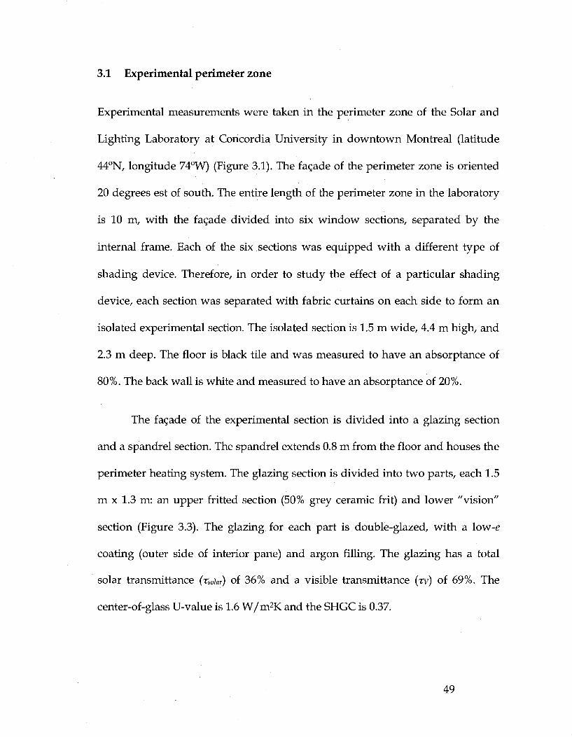
3.1 Experimental perimeter zone

Experimental measurements were taken in the perimeter zone of the Solar and

Lighting Laboratory at Concordia University in downtown Montreal (latitude

44°N, longitude 74°W) (Figure 3.1). The facade of the perimeter zone is oriented

20 degrees est of south. The entire length of the perimeter zone in the laboratory

is 10 m, with the fagade divided into six window sections, separated by the

internal frame. Each of the six sections was equipped with a different type of

shading device. Therefore, in order to study the effect of a particular shading

device, each section was separated with fabric curtains on each side to form an

isolated experimental section. The isolated section is 1.5 m wide, 4.4 m high, and

2.3 m deep. The floor is black tile and was measured to have an absorptance of

80%. The back wall is white and measured to have an absorptance of 20%.

The facade of the experimental section is divided into a glazing section

and a spandrel section. The spandrel extends 0.8 m from the floor and houses the

perimeter heating system. The glazing section is divided into two parts, each 1.5

m x 1.3 m: an upper fritted section (50% grey ceramic frit) and lower "vision"

section (Figure 3.3). The glazing for each part is double-glazed, with a low-e

coating (outer side of interior pane) and argon filling. The glazing has a total

solar transmittance (xSoiar) of 36% and a visible transmittance (xv) of 69%. The

center-of-glass U-value is 1.6 W/m2K and the SHGC is 0.37.

49

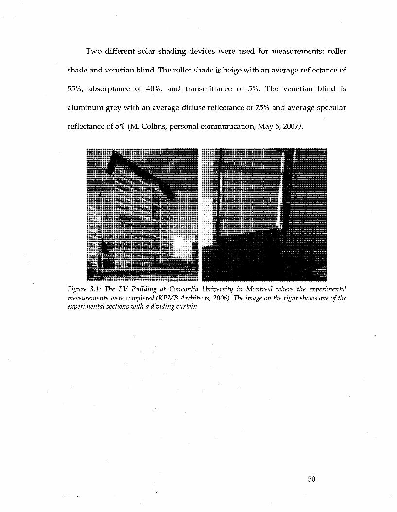
Two different solar shading devices were used for measurements: roller

shade and Venetian blind. The roller shade is beige with an average reflectance of

55%, absorptance of 40%, and transmittance of 5%. The Venetian blind is

aluminum grey with an average diffuse reflectance of 75% and average specular

reflectance of 5% (M. Collins, personal communication, May 6, 2007).

Figure 3.1: The EV Building at Concordia University in Montreal where the experimental measurements were completed (KPMB Architects, 2006). The image on the right shows one of the experimental sections with a dividing curtain.

50

/

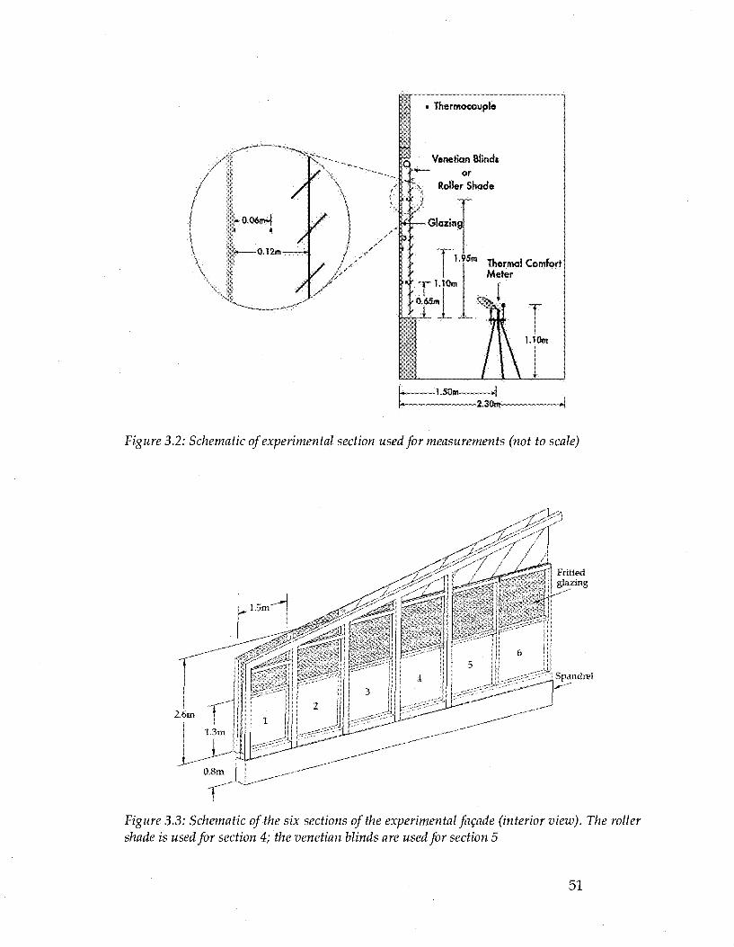
|» O.Wro*|

-0.12m-

/

• Thermocouple

Venetian Blind* -'* or

Roller Shade

pr-

•Glazing

,' 0.65m

1 ' ? S m Thermal Comfort Meter

1.10m

~2.30m———-——•(

Figure 3.2: Schematic of experimental section used for measurements (not to scale)

^aa

2.6o\

Fritted glazing

Spandrel

1.3m

0.8m

Figure 3.3: Schematic of the six sections of the experimental fagade (interior view). The roller shade is used for section 4; the Venetian blinds are used for section 5

51

3.2 Data acquisition system, sensors, and measurements

Climatic data was collected from exterior sensors placed outside next to the

laboratory. Solar radiation incident on the facade was recorded using a Li-cor

pyranometer. It is pre-calibrated against an Eppley precision spectral

pyranometer under natural conditions. It has a spectral response from 280 - 2800

ran, a linear response up to 3000 W/m 2 , a cosine correction for an angle of

incidence up to 80°, a response time of 0.01 ms, and an absolute error of 3%.

Several T-type thermocouples (error = ±0.5 °C) were used to record the exterior

air temperature. Thermocouples were also used to record the temperatures of all

the interior surfaces (glazing, shading device, floor), the air gap between the

glazing and shading device, and indoor air temperature. For the interior glazing

surface, three thermocouples were used: in the center of the bottom vision

section, 10 cm below the horizontal window frame in the bottom vision section,

and the center of the upper fritted section. A thermocouple was placed below the

horizontal window frame in the bottom section because the frame could act as a

shade on part of the window during times of high solar altitude.

Indoor environmental conditions were measured using a Briiel & Kjaer

Indoor Climate Analyzer (Type 1213), which is a collection of instruments and

transducers that can measure individual indoor environmental parameters: air

velocity, humidity, temperature, and plane radiant temperature (Figure 3.4).

Plane radiant temperature is measured using a net radiometer. It consists of a

small black plate element with a heat flow meter (thermopile) between the two

52

sides of the element. The radiant temperature asymmetry can be estimated by the

difference in net heat flow between the two sides of the element. A thin

polyethylene sphere covers the element to minimize the effect of air velocity

(Blazejczyk et al., 1998).

(a) « (c) W

Figure 3.4: Instruments for measuring indoor environmental parameters: (a) air velocity; (b) shielded air temperature; (c) humidity; (d) plane radiant temperature. (Parsons, 2003)

No method exists for a direct measurement of MRT, although many

prototype instruments have been developed such as a normal globe

thermometer, polyethylene shield globe, and two- or three-sphere radiometer.

The most common method for measuring MRT is the use of a black globe, which

consists of a hollow, black sphere with a temperature sensor in its center.

However, the globe shape (sphere) and colour (black) do not accurately represent

the shape of a person or colour of clothing. Therefore, the use of an ellipsoid-

shaped sensor is the preferred since its projected area factors may be considered

a closer approximation of the shape of a human body. In a study testing the

effect of solar radiation on an ellipsoid-shaped sensor, it was determined that

measurements were most accurate when the sensor was a grey colour

53

(Blazejczyk et al., 1998). For this reason, a Briiel & Kjaer Thermal Comfort Meter

(Type 1212) consisting of a grey-coloured ellipsoid-shaped transducer was used

to measure the operative temperature. It was set at a 30° angle from the

horizontal, to closely match the ratio of radiative heat loss to convective heat loss

of a seated human body. The indoor climate analyzer and thermal comfort meter

were placed 1.3 m from the fagade at a height of 1.1 m.

Data was collected every minute from the exterior and interior sensors and

transducers for a period of three months, from January to March 2007. The

objective was to examine the impact of climatic conditions and shading devices

on thermal comfort conditions near the fagade during sunny and cloudy days.

Therefore, the perimeter heating was turned off so that quasi-free-floating

environmental conditions of the perimeter zone could be measured (although

the section was affected by small air exchanges with the adjacent core zone of the

laboratory as a result of small gaps between the curtains and floor/ceiling). The

results of the measurements were also used to validate the simulation model

(Chapter 4). The results for clear and cloudy representative days are presented in

the next section.

54

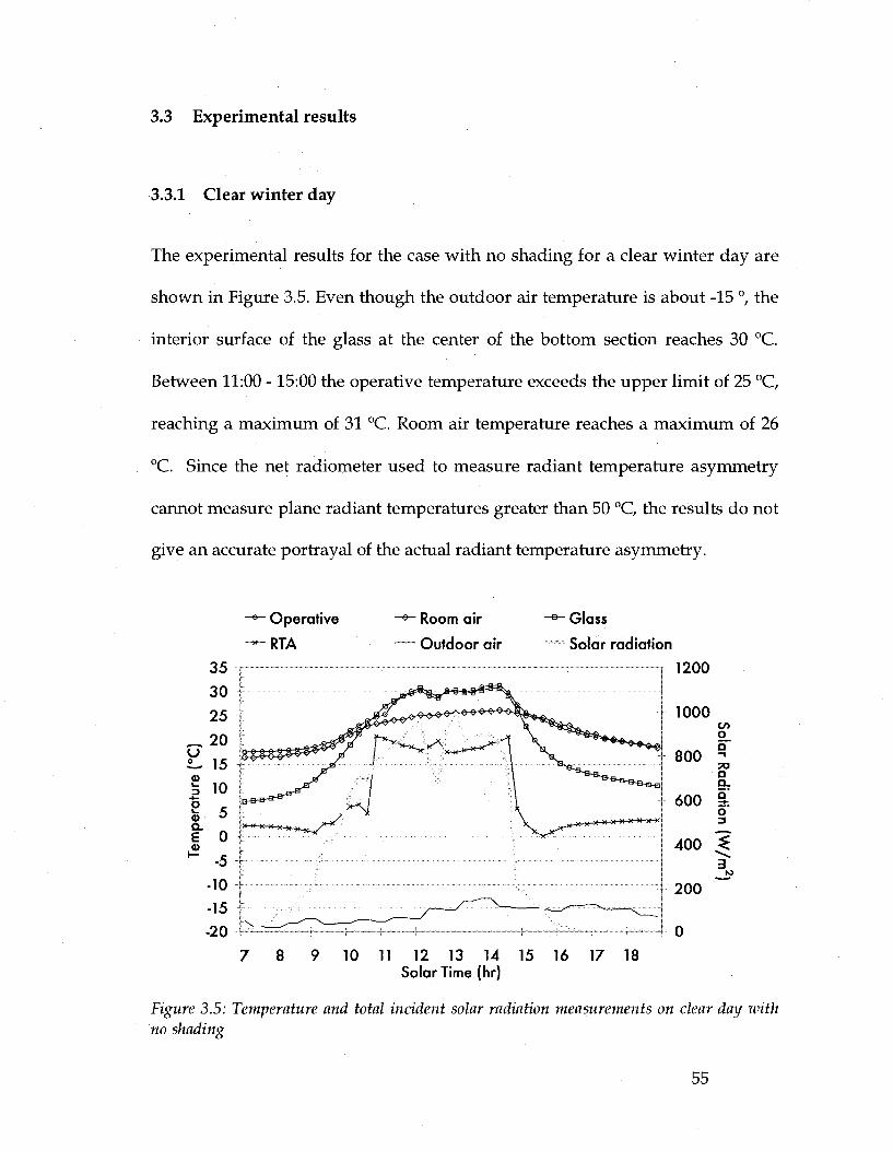
3.3 Experimental results

3.3.1 Clear winter day

The experimental results for the case with no shading for a clear winter day are

shown in Figure 3.5. Even though the outdoor air temperature is about -15 °, the

interior surface of the glass at the center of the bottom section reaches 30 °C.

Between 11:00 - 15:00 the operative temperature exceeds the upper limit of 25 °C,

reaching a maximum of 31 °C. Room air temperature reaches a maximum of 26

°C. Since the net radiometer used to measure radiant temperature asymmetry

cannot measure plane radiant temperatures greater than 50 °C, the results do not

give an accurate portrayal of the actual radiant temperature asymmetry.

Operative

RTA

Room air

Outdoor air

Glass

Solar radiation

1200

1000

800

600

400

200

o_ ar Radi

1 (W/m

2

7 8 9 10 11 12 13 14 15 16 17 18 Solar Time (hr)

Figure 3.5: Temperature and total incident solar radiation measurements on clear day with no shading

55

When using a roller shade on a sunny day with slightly higher outdoor

temperatures (Figure 3.6) both the shade and the interior surface of the window

reached temperatures over 40 °C. However, since the shading device reduces the

transmittance of direct solar radiation into the space, conditions remained within

the comfort zone for most of the day (9:30 - 18:00). During this time period, the

operative temperature was held between 20 - 26 °C, RTA remained at or below 5

°C, and the room air remained between 22 - 25 °C.

- * - Operative

— Outdoor air 45

Roller shade - * - Glass -* - Room air

RTA Solar radiation 1200

7 8 9 10 11 12 13 14 15 16 17 18 19

Solar Time (hr)

Figure 3.6: Temperature and total incident solar radiation measurements on a clear day with roller shade

With the Venetian blind set at a horizontal position (slat tilt angle = 0°) on

a similar cold and sunny day (Figure 3.7), the glazing and blind reached

temperatures of 32 °C. Since the blind slats are in a horizontal position, part of

the beam solar radiation is directly transmitted into the office. This can be

56

observed from the radiant temperature asymmetry results. Again, since the net

radiometer cannot record plane radiant temperatures greater than 50 °C, the

maximum RTA is only shown to be around 23 °C although it is expected to be

much higher in reality. The "spikes" in the RTA value are due to intermittent

shading of beam solar radiation on the net radiometer by the individual blind

slats. An occupant would not experience these intermittent decreases in RTA

since the surface of a human body is larger than the net radiometer and would

therefore be simultaneously shaded and irradiated. The operative temperature

remained above the comfort zone from 11:00 - 17:00, reaching a maximum of 31

°C. During this time, room air temperature ranged from 23 - 27 °C.

*- Operative

^RTA 40

-5 -10 -15 -20

- * - Room air

— Outdoor air

Glass - * - Venetian blind

Solar radiation 1200

1000

800

600

400

200

0

Sol ar R

adi

1 ? 3

7 8 9 10 11 12 13 14 15 16 17 18 19 Solar Time (hr)

Figure 3.7: Temperature and total incident solar radiation measurements on a clear day with Venetian blind (tilt = 0°)

57

Positioning the blind slats to a tilt of 45° has a significant effect on the

thermal environment since it can decrease the amount of direct solar radiation

entering the office (Figure 3.8). This can be seen in the significant reduction in

RTA. The RTA is kept below 10 °C for the entire day, except for small

intermittent increases in the afternoon when the sun's altitude is lower. The

glazing reaches a maximum temperature of about 32 °C while the blind reaches

slightly higher at 33 °C. Between 10:00 - 18:00 the operative temperature is

maintained between 21 - 27 °Q exceeding the comfort zone between 12:30 -

16:30. During this time the air temperature ranges from 20 - 25 °C.

Operative

RTA

Room air ~a~ Glass - * - Venetian blind

Outdoor air Solar radiation

1200

8 9 10 11 12 13 14 15 16 17 18 19 20 Solar Time (hr)


Tilting the slats 90° to a closed position creates a vertical barrier between

the glazing and indoor space (Figure 3.9). In this position the blind reaches a

58

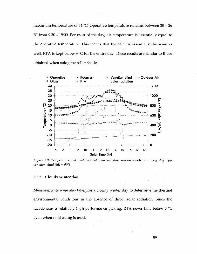
maximum temperature of 34 °C. Operative temperature remains between 20 - 26

°C from 9:30 -19:00. For most of the day, air temperature is essentially equal to

the operative temperature. This means that the MRT is essentially the same as

well. RTA is kept below 3 °C for the entire day. These results are similar to those

obtained when using the roller shade.

»- Operative a- Glass

40

35

Room air RTA

Venetian blind Solar radiation

30

£ 2 0

g 15

1 10 a. 5

I 0

-10

-15

-20

Outdoor Air

1200

X-X X n H'X-XiHfH-* - * - * v „ t"X-X-M"X"H-X'

1000

o_

800 ° TO a a.

600 I o

4 0 0 ^

200

0

6 7 8 9 10 11 12 13 14 15 16 17 18 Solar Time (hr)


3.3.2 Cloudy winter day

Measurements were also taken for a cloudy winter day to determine the thermal

environmental conditions in the absence of direct solar radiation. Since the

facade uses a relatively high-performance glazing, RTA never falls below 5 °C

even when no shading is used.

59

Figure 3.10 presents results for the case with no shade. The interior surface

of the glazing ranges between 13 - 19 °C from 9:00 - 17:00. Room air and

operative temperature ranges between 18 - 21 °C and RTA is kept below 5 °C

during this time.

With the Venetian blind at a horizontal position (slat tilt = 0°) the room air,

blind, and operative temperatures remained between 16 - 19 °C and glazing

interior temperature remained between 11 - 1 3 °C for most of the day, while RTA

does not exceed 4 °C.

Tilting the slats to an angle of 45°, operative temperature is between 20 -

23 °C and room air temperature is between 17 - 22 °C. RTA remains below 5 °C.

With the blinds fully closed (slat tilt = 90°), operative temperature never

falls below 20 °C.

60

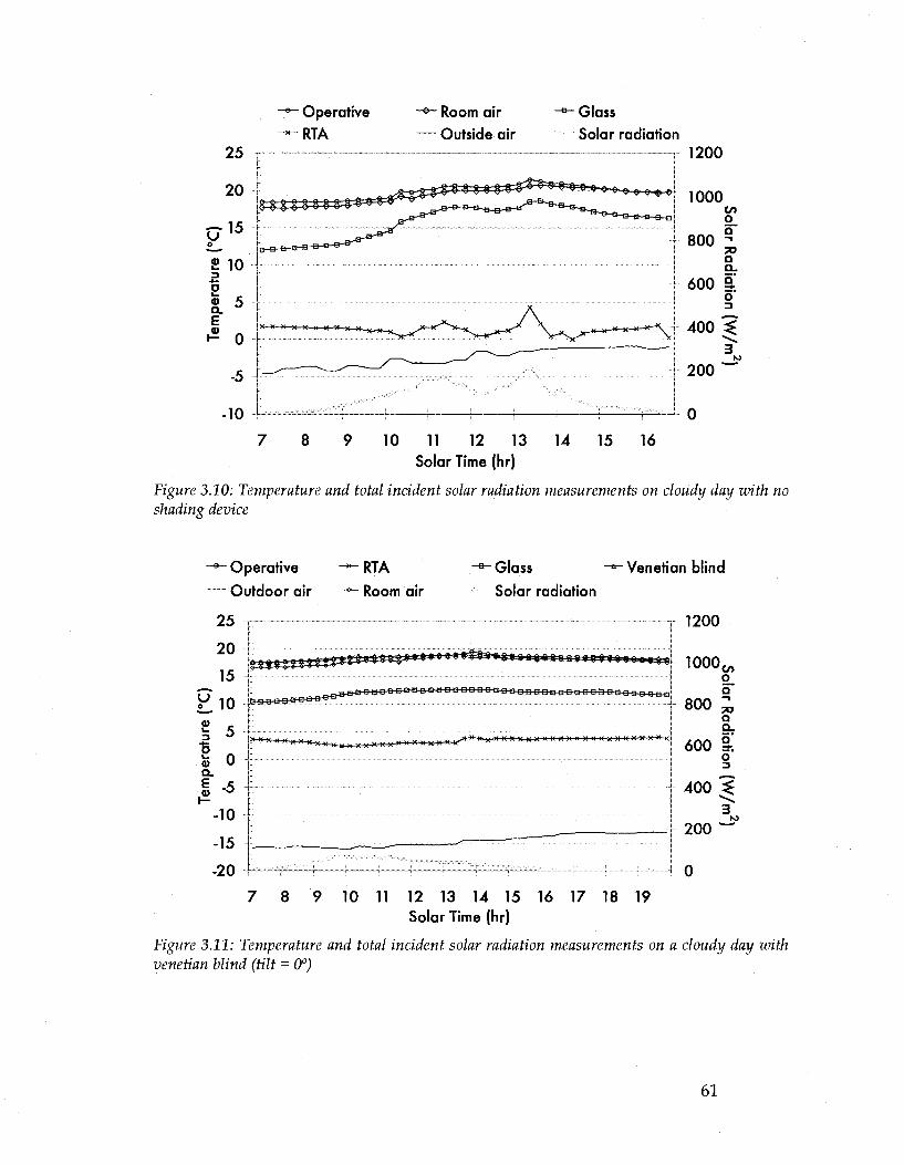
Operative

RTA

-*~ Room air

— Outside air

Glass

Solar radiation 25

20

U 1 5

£ 10 3 e c g. 5 E

»= 0

-5

-10

X X X X- H )( )< X x K-

1200

1000 CO

o_ 800 °

50 Q Q_

600 a o 3

400 ^

"3* 200 ~

7 8 9 10 11 12 13 14 15 16 Solar Time (hr)

Figure 3.10: Temperature and total incident solar radiation measurements on cloudy day with no shading device

Operative

Outdoor air

RTA

Room air

ntssnzzn*************

Glass -*- Venetian blind

Solar radiation

1200

1000

j - f i n q n n D D D D O a n a n n n n D n n n n r m n p n g n n n n n n a o n a a

c n x H x n M-J**~* * " " " " " " " " " " " " " " " * x)< )<)( x-x

25

20

15

£io 1 5 § 0 a. E -5

-10

-15

-20 7 8 9 10 11 12 13 14 15 16 17 18 19

Solar Time (hr)

Figure 3.11: Temperature and total incident solar radiation measurements on a cloudy day with Venetian blind (tilt = 0°)

800

600

'CO 0 0

TO O

a. Q_

0 3

400 ^

200 3 •—•

61

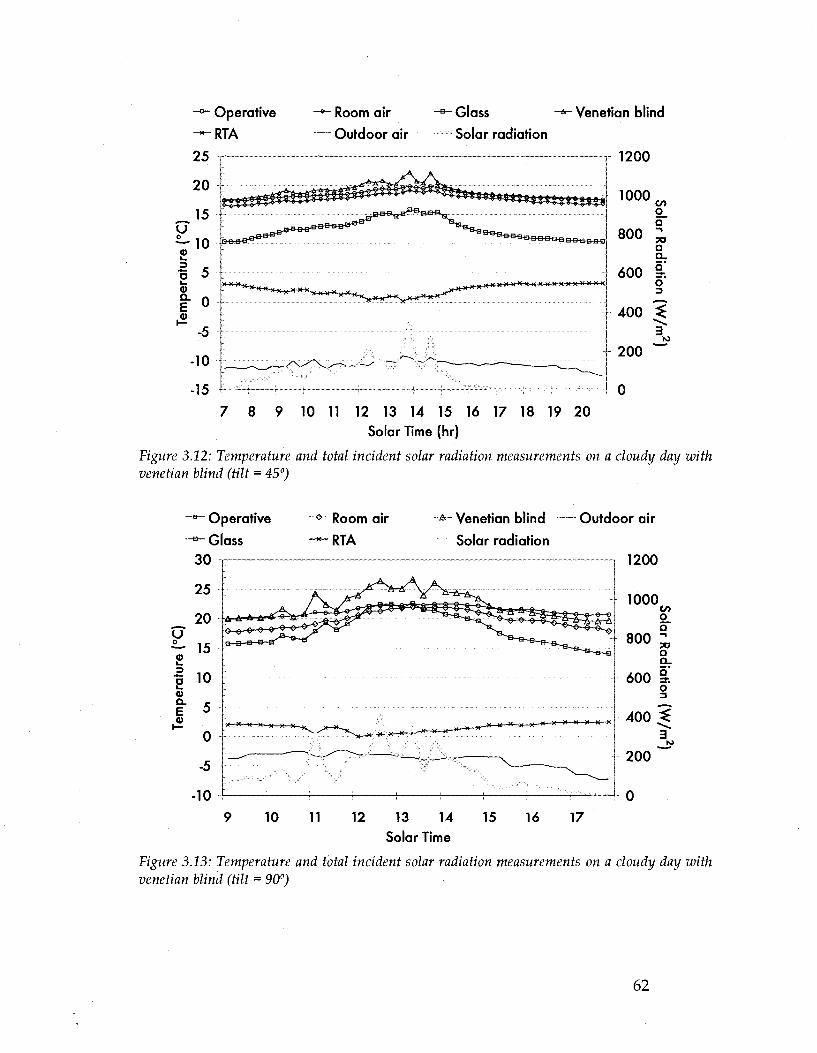
Operative

RTA

25

20

_ 1 5 u

4)

1 5 i .

-5

-10

-15

Room air

Outdoor air

Glass

Solar radiation

Venetian blind

1200

&&&s'Q«&afH3-d

j-M-H M X M H-M )( K )(X X X X X-X-X-Xj

1000

800 I 600 §,

o

400 ^

200

0

7 8 9 10 11 12 13 14 15 16 17 18 19 20

Solar Time (hr)


Operative

Glass

30

-10

Room air - * - Venetian blind — Outdoor air

RTA Solar radiation

1200

1000

800

o_ o -1 TO O Q.

600 o 3

400^

200

0 10 11 12 13 14

Solar Time

15 16 17


62

3.4 Summary

The results of the experimental study show how outdoor climate affects indoor

environmental and comfort conditions. The results also show how shading

devices impact these conditions.

Using a roller shade on clear winter days can improve the indoor thermal

environment (operative temperature and radiant temperature asymmetry) by

minimizing the amount of direct solar radiation absorbed by the occupant. Using

Venetian blinds on clear winter days can also improve the indoor thermal

environment but is dependent on the tilt angle of the slats. Maintaining slat

angles at a horizontal position (tilt = 0°) can still cause discomfort since a large

amount of the incident beam solar radiation can still be transmitted into the

space. A tilt of 45°, however, will decrease the amount of beam radiation entering

the space and will, therefore, improve the indoor environment.

On cloudy winter days it was shown that shading devices can decrease the

amount of heat loss through the facade and improve the thermal environment of

the space. Once again, the Venetian blinds set at a horizontal position showed no

discernable effect compared with having no shading device since it shields only a

small fraction of the glazing.

These results, however, are specific to the experimental facade. Even if the

building envelope and blind properties are kept the same, a building at different

latitude and with different orientation will have different results due to variation

63

in incident solar radiation. The purpose of the experimental study was to

develop a general understanding of the impact of shading on indoor

environmental conditions and to compare results with those generated with a

numerical simulation study, which will be described and discussed in the next

chapter. This numerical simulation study presents a model with which indoor

environmental conditions can be assessed for different building envelope and

blind properties and facade location and orientation.

64

4 NUMERICAL SIMULATION STUDY

This chapter presents the description and results of a numerical simulation study

of a thermal analysis of a typical office in a highly glazed perimeter zone and its

impact on thermal comfort. The results of the simulation study are compared

with the experimental results discussed in Chapter 3. A numerical thermal

simulation model of a typical office was developed using the Mathcad

simulation software. A parametric analysis of the thermal response of the office

was completed for different fenestration component properties (glazing and

roller shade) and different climatic conditions. A numerical simulation study of

thermal comfort was completed based on a transient two-node thermal comfort

model. The results of the thermal comfort simulation are compared with

experimental results found in the literature. Further investigation into the impact

of heated air supply on airflow and comfort conditions using Computational

Fluid Dynamics (CFD) is also presented.

4.1 Description of thermal simulation model

A transient building thermal simulation model of a typical office in a highly

glazed perimeter zone was developed using the Mathcad simulation software. In

Mathcad, the source code of the simulation program can be written in the form of

mathematical expressions. The model uses the explicit finite-difference thermal

65

network approach. The entire simulation model is built upon several

components:

• Typical Meteorological Year (TMY) weather data

• Solar radiation (Perez model)

• Geometry of perimeter zone office and angle factors

• Solar radiation transmission through glazing

• Building thermal simulation

• Thermal environmental conditions

• Transient thermal comfort modeling

4.1.1 Typical meteorological year weather data

An hourly weather data file for a Typical Meteorological Year (TMY) for

Montreal was imported from an Energy Plus weather file database for use in the

thermal simulation. The file contains hourly data for climatic variables including

horizontal beam and diffuse irradiance, dry-bulb air temperature, dew-point

temperature, humidity ratio, and wind speed.

4.1.2 Solar radiation model

The parameters in the simulation are expressed as a function of Julian day

number (n) and solar time (t). Hourly values of solar position are determined by

a three-dimensional angle with spherical coordinates based on longitude,

latitude, altitude, surface azimuth (ip), surface tilt angle (/3), solar altitude (a), and

solar azimuth (<p) (Figure 4.1). These angles are a function of day number and

66

solar time. The solar incidence angle is the angle between the sun's rays and a

line normal to the surface, calculated by (Athienitis, 1998):

0(n, t) = cos"1 [cos(a(n, t)) • cos(cp(n, t)-xp)- sin(/?) - sin(ot(n, t)) • cos(/S)] (4.1)

Hourly incident solar radiation on a tilted surface (fagade) is calculated

from horizontal irradiance values. Direct beam solar radiation on a tilted surface

is calculated from:

Ib{n,t) = Ibn{n,tycos{e(n,t)) (4.2)

where hn is the direct beam normal irradiance.

EARTH-SW Lim

Figure 4.1: Solar angles for vertical and horizontal surfaces (ASHRAE Handbook of Fundamentals, 2005)

67

Diffuse sky radiation on a tilted surface is calculated using the Perez

diffuse irradiance model (Perez et al., 1990). It consists of three components:

1. Isotropic part, received uniformly from the entire sky dome

2. Circumsolar diffuse, resulting from forward scattering of solar radiation and

concentrated in the part of the sky around the sun

3. Horizon brightening, concentrated near the horizon and most pronounced

in clear skies

The portion of diffuse irradiance coming from the sky can be calculated by:

Ids(n,t) = Idh(n,t)- ( 1 - F J - l ^ ^ l + F ^ + V s i n / ? (4.3)

where:

Idh = sky diffuse horizontal irradiance;

Fi = circumsolar brightening coefficient;

F2 = horizon brightening coefficient;

a - horizon brightness coefficient;

b = horizon brightness coefficient;

The brightening coefficients are statistically derived and represent the

degree of sky anisotropy. They are a function of solar altitude, sky clearness, and

sky brightness.

The component of diffuse radiation that is reflected from the ground (Idg)

is calculated by:

68

T /T T \ l - c o s / 5

where hh is the beam horizontal irradiance and pg is the ground reflectance

(albedo).

The total hemispherical diffuse solar radiation on a tilted surface (Id) is the

summation of the sky diffuse component and the ground-reflected diffuse

component:

Therefore, the total irradiance incident on a tilted surface is:

I-!„+!, (4.6)

^WZ* v *; isotropic i diffuse

X

x%% «<h \ \ ^ X %

% X X XX^Jb ' d

N x ' , y "onzo^tal diffuse

Figure 4.2: Direct radiation, ground reflected radiation, and different components of diffuse radiation (Fieber, 2005)

69

4.1.3 Geometry of perimeter zone office

The geometry of the office is needed for calculation of the view factors between

each surface, which, in turn, is needed for radiation heat transfer calculation. The

view factor from surface i to surface j (F,y) is equal to the fraction of diffuse

radiation leaving surface i that is directly incident on surface j . For two

perpendicular rectangles with a common edge, the view factor is given by

(Athienitis, 1998):

F * - TfW

1 \ I 1 w • tan_1| — \ + h- tan"1'

w iy^ w2 • tan-1

+hn\ (l + w2)(l + h2)

l + w2 + h2

w2(l + w2 + h2)

(l + w2)(w2 + h2)

^h2 + w2)

h2(l + h2 + w2)

(l + h2)(h2 + w2)

(4.7)

where h = Z/X and w = Y/X

For two parallel rectangular surfaces, the view factor is given by:

F„ jr-w-h

ll + h2)(l + w2) ,

V l + h2 + w2 w2 tan 1

IVIT w

+icnjl + h2 tan-1 w \4i^j

-/ztan 1(/ij-tytan 1[w\

(4.8)

where h = X/L and w = Y/L

70

1 0.2 0.5 t

A, PERPENDICULAR RECTANGLES WITH COMMON EDGE B. ALIGNED PARALLEL RECTANGLES

Figure 4.3: Graphical representation of view factors for radiation heat transfer calculation (ASHRAE Handbook of Fundamentals, 2005)

The view factors between all the room surfaces are calculated by applying

the follow principles (Athienitis, 1998):

Reciprocity:

Symmetry:

Airij — Ajtji

Fij = Fik

Energy Conservation: V F(j =1

(4.9)

(4.10)

(4.11)

4.1.4 Solar radiation transmission through glazing

Typically, transmission of solar radiation into the interior space through non

opaque elements such as windows is calculated using the laws of optics. This

method determines reflectance, absorptance and transmittance based on the

element's thickness, extinction coefficient, refractive index, and angle of

incidence. However, for the purposes of this simulation study, the glazing that

71

was used exhibit complex optical properties due to their selective coatings and

tints. Therefore, solar-optical properties (absorptance, transmittance, and

reflectance) were determined using the properties given in ASHRAE Handbook

of Fundamentals (2005) which are given as a function of incidence angle for

beam and diffuse radiation for each glazing layer.

Heat transfer through the fenestration system is determined by its U-value

and is a function of the U-value for the window frame, edge-of-glass, and center-

of-glass. For a curtain wall with aluminum frame, thermal break, and insulated

spacer the frame U-value (Uf) is taken to be 9.26 W/m2K for all glazing types.

The edge-of-glass effects are assumed to extend over a 65 mm-wide band

around the perimeter of the glazing. The U-value for the edge-of-glass (Ueg) can

vary from 2.49 W/m2K for low-e triple-glazed windows to 3.36 W / m 2 °c for clear

uncoated double-glazed windows (ASHRAE Handbook of Fundamentals, 2005).

The center-of-glass U-value (Ucg) for double- and triple-glazed windows is

approximately equal to the sum of the convective and radiative heat transfer

coefficients between the panes of glass. For parallel plates, the convective heat

transfer coefficient across a rectangular cavity is related to a number of

dimensionless parameters: the Nusselt number (Nu), the Rayleigh number (Ra),

and the Prandtl number (Pr) (ASHRAE Handbook of Fundamentals, 1989). The

convective heat transfer coefficient (hc) is determined by:

72

h - \ ^•(Nu1)i£Nu1>Nu2

air

L •(NM2) if Nut ^Nu2

(4.12)

where fc«,y is the thermal conductivity of air and L is the length of the cavity. The

thermal conductivity of air is calculated by:

k _ 0.002528 -Tmea

T _ + 200

1.5

(4.23}

where Tmean is the mean temperature of the hot and cold plates (°C). The Nusselt

number is calulcated by:

Nul=0.0605(Raf/3 (4.14)

Nu2 = + -

/ \ 0.293

0.104(Rfl)

1 + / \1.36'

[63101

3

1/3

(4.25)

For air the Rayleigh number, Ra, is determined by:

Ra = 2.737(1 + 2a)2 • a4 • (TM - TcM )(l)3 • p2 (4.16)

where p is the pressure in atmospheres, and a equals 100°C/rra

Therefore, the overall U-value (L70) for a fenestration system becomes:

73

^ m UcAg

+Ueg\+UfAf (417)

4.1.5 Building thermal simulation model

The building thermal simulation model uses the previous four modules (weather

data, Perez irradiance model, room geometry and view factors, and solar

transmission through glazing) as inputs. An explicit finite difference thermal

network approach is used to simulate the transient thermal response of a

perimeter zone office. The thermal network approach discretizes the space into a

series of nodes with interconnecting paths through which energy flows. Thermal

networks depend on a heat balance at each node to determine its temperature

and energy flow between all connected nodes. Finite difference models are one of

the most efficient techniques used for building simulation purposes

(Tzempelikos, 2005).

For this simulation, each surface, mass layer, and air component is

represented by a node that is connected by one or more thermal resistances to

other adjacent nodes (Figure 4.4). The thermal resistances in the network (R)

represent the three heat flow mechanisms between two nodes: convection,

radiation, and conduction. Non-linear heat transfer coefficients for convection

and radiation are employed; therefore, resistances are a function not only of

temperature, but also of time. Solar radiation absorbed in each layer is

74

represented by sources (S) and heat storage in thermal mass is represented by

capacitances (Q.

0 - Exterior air temperature 1 -Exterior window surface 2 -hteriorwBidowsurface

3 -Exteriorwall outside surface 4 -Exteriorwall mass 5 -Exteriorwall inside surface 6 - R O O T surface 7-Roor mass 8 - Wails interior surface 9-Wails mass 10-RoomAir 11 — Roller shade 12-A i rgap (befcweenshadeandwindow ) 13 - Ceiling 14-Ceil ing mass 15 - Adjacent Room Air R-Resistance C -Capactence S -Heatsource

Figure 4.4: Thermal network diagram of perimeter zone office

Conduction heat transfer is a function of a material's thermal conductivity

(k), area (A), and thickness (L), and is thus calculated by:

R = L/kA (4.18)

The convection heat transfer coefficient for interior surfaces is a function

of the surface temperature of the element (Ts) and the surrounding air (Ta) and

can be calculated as:

75

/zc=1.3l(Ts-Tfl)1/3 (4.19)

Radiation heat transfer between all surfaces is modeled in detail using the

radiosity method. Radiation view factors between surfaces are calculated and

radiation heat exchange is represented with non-linear heat transfer coefficients.

It is calculated by:

*„-"*f:Ty <**» where o is the Stefan-Blotzmann constant, F-- is the radiation exchange factor

(script F) for the two surfaces (a function of view factors and emissivities) and T,

and Tj are the temperatures of surfaces i and j (degrees K), respectively.

Radiation exchange factors between surfaces are a function of their

respective emissivities (s):

r . . * - - ; — (^-21)

1-1 e,i) , x

\£' EH

For common building materials, emissivity is 0.9; low-e coatings on

glazing can have an emissivity as low as 0.05.

The total exterior heat transfer coefficient is the sum of the convection and

radiation coefficients following the Energy Plus approach (Bauman et al., 1983).

76

The total convection coefficient is a combination of natural and forced convection

coefficients, with the natural convection coefficient calculated by:

1.81-3/T - T h = * - ! °- (4.22)

1.382

where T0 is the outside air temperature (°C). The total exterior convective heat

transfer coefficient depends on the roughness of the surface exposed to the

outside air (Bauman et al., 1983):

hcogkss = yjhl + (a • vl )2 for smooth (glass) surfaces (4.23)

hco =hn+Rf-(hcoglass -h0) for rough (cladding) surfaces (4.24)

where a and /? are constant modifiers for forced convection, v0 is the wind speed,

and Rf is a surface roughness coefficient (1.6 for brick/concrete). The exterior

radiation coefficient is a function of the temperature of the sky and the ground

and their respective view factors. For simplicity, linearization is used:

hro=4-a-ss-T^ (4.25)

where ss is the effective emissivity of the exterior surface and Tm is the mean

temperature of the sky, ground, and surface temperature. Therefore, the total

exterior heat transfer coefficient is evaluated for each exterior surface and is

calculated by:

&„=&*,+&„ (4-26)

77

Heat storage in the building structure (walls, floor, ceiling) is modeled by

using one or more thermal capacitances in the building mass nodes. The thermal

capacitance (C) is calculated by:

C = cp-p-Vol (4.27)

where cv is the specific heat, p is the density, and Vol is the volume of each mass

node.

The amount the solar radiation transmitted into the perimeter zone office

is computed based on the hourly values of direct and diffuse solar radiation

incident on the facade and the optical properties of the window system. The

optical properties of the glazing depend on the type used, as described above.

The roller shades are assumed to be perfect diffusers with constant transmittance

(5%) over all wavelengths.

An energy balance is applied at each node for each time-step to determine

the temperature of each node as a function of time. The system of simultaneous

differential and algebraic non-linear equations is then solved numerically in

Mathcad using an explicit finite difference technique. This involves going

forward in time based on a set of initial conditions. The general form of the

explicit finite difference model corresponding to node i and time-step p is

(Athienitis, 1999):

78

„p+1 _ At )

c IJV_JA

+ T," (4.28)

where T is the temperature, p+1 represents the next time-step, j represents all

nodes connected to node i, Rij is the thermal resistance connected nodes i and ;', Q

is the capacitance of node i, and q is a heat source at node i. Using this equation,

temperatures of all nodes are calculated at each time-step. The heating and

cooling load is computed using appropriate proportional and integral control

constants. Heating and cooling, if needed, is applied directly to the air node.

A short simulation time-step (five minutes) was selected based on

numerical stability criteria. Since the thermal simulation must run on a five-

minute time-step, the values of all simulation parameters must also be re

evaluated every five minutes. To do this, all parameters with hourly values were

modelled by discrete Fourier Series and then applied with an inverse Fourier

transform for the time-step (Athienitis, 1999).

4.1.6 Indoor thermal environment

Once the building thermal simulation model has computed the interior surface

temperatures, air temperature, and transmitted solar radiation into the space at

each time-step, it is possible to determine the mean radiant temperature,

operative temperature, and radiant temperature asymmetry.

79

To determine the mean radiant temperature, the view factors between a

seated person and the surrounding surfaces (FP-A) are computed using a

calculation method developed by Cannistraro et al. (1992):

FP-A = FMAx(l-exp[-(fl/c)T])- il-exp[-(b/c)/y]) (4.29)

where:

r=A+B- (4.30)

y=C + D- + E- (4.31) c c

The coefficients a, b, and c are show in Figure 2.1. The coefficients A, B, C,

D, and E can be found in Appendix D.

To determine the mean radiant temperature of a person irradiated by

solar radiation, the projected area factor (fp) of the sun on the person is computed

using a method developed by Rizzo et al. (1989):

/p(a,/3) = 2A(^)-«; (4-32)

A(/*) = i A , r £ ; (4-33) 7-0

80

where a is the azimuth angle between the front of the seated person and the sun

and /3 is the solar altitude angle. The values for the coefficient Ay can be found in

the Appendix E.

The mean radiant temperature for a person exposed to solar radiation is

then calculated using the algorithm developed by La Gennusa et al. (2005)

described in detail in Chapter 2:

,4 v « „ m 4 1 / M \

£*0 *-r ~ 2j P~> { + airr,d 2j P-)d'i +Clirr'b^Pb (4.34)

4.2 Comparison of thermal simulation model and measurements

The simulation model was compared with the results of the experimental

measurements by using the climatic data from the measurements as inputs. The

parameters used in the simulation for verification were modeled after the

experimental fagade section and therefore not considered to be representative of

a "typical" office. For example, the interaction between the conditioned adjacent

core zone and the unconditioned experimental section due to the divisions

between the sections had to be taken into account. Nevertheless, adequate results

could be generated using these parameters.

It should also be noted that verification of the experimental measurements

were only completed for the cases with the roller shade and not for the Venetian

81

blind, because there is currently no available method for calculating view factors

between a person and complex surfaces such as tilted Venetian blinds.

4.2.1 Clear winter day: no shading

The following figures show a comparison of simulation results with measured

values for a clear winter day with no shading. It can be seen from Figure 4.5 that

the operative temperature in the simulation model increases quicker than with

the measured data in the morning while the measured data decreases quicker at

the end of the day. This could be due to greater surface-solar azimuth angles at

sunrise and sunset that caused partial shading of the thermal comfort meter that

was not taken into account in the model.

35

_ 30 u o

£ 25 •4—

O

© 20 Q-

E £ 15 ©

8 10 © Q.

° 5

Simulation Experimental Solar Radiation 1200

1000 CO

o_

800 1 TO Q a_ 600 I! o

400 ^ 3

200

0

7 8 9 10 11 12 13 14 15 16 17 18 19 20 Solar Time (hr)

Figure 4.5: Operative temperature: verification of simulation model with measured values for a clear winter day with no shade

82

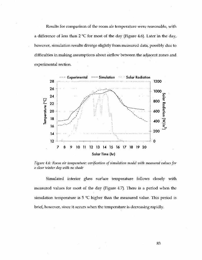
Results for comparison of the room air temperature were reasonable, with

a difference of less than 2 °C for most of the day (Figure 4.6). Later in the day,

however, simulation results diverge slightly from measured data, possibly due to

difficulties in making assumptions about airflow between the adjacent zones and

experimental section.

28

26

~ 24 u — 22 £ •§ 20 c Q>

§- 18 0)

h-16

14

12

- Experimental Simulation - ; —

/ ^ *S. ^ • — , .

s /

'/ // //

/ / 1

/ 1 / 1

/ /

^ ^ ^ • -

Solar Radiation "-

\ \

\ ~—-— X

\ . . . . • -s...

. , ,,-.

1200

1000 c/> o Q

800 2, 70 Q Q_

600 §! o 3

400 "? * s , N t ,

3

200

0

7 8 9 10 11 12 13 14 15 16 17 18 19 20

Solar Time (hr)

Figure 4.6: Room air temperature: verification of simulation model with measured values for a clear winter day with no shade

Simulated interior glass surface temperature follows closely with

measured values for most of the day (Figure 4.7). There is a period when the

simulation temperature is 5 °C higher than the measured value. This period is

brief, however, since it occurs when the temperature is decreasing rapidly.

83

Experimental Simulation Solar Radiation

u o

£ D •*-• o l_ <D

a. E £

*-\*

20

15

10

1200

1000

800

600

400

200

o a -% 73 a a. 5' 5" 3

g "^ 3 K>

7 8 9 10 11 12 13 14 15 16 17 18 19 20 Solar time (hr)

Figure 4.7: Interior glass surface temperature: verification of simulation model with measured values for a clear winter day with no shade

4.2.2 Clear winter day: roller shade


values for a clear winter day when using a roller shade. Figure 4.8 shows that the

simulation results for operative temperature has a maximum difference of 2 °C

from measured values. Simulated room air temperature follows closely with

measured values except after 18:30 when there is a difference of over 3 °C. This

could be due to difficulties in trying to model the airflow between the core zone

and experimental zone correctly (Figure 4.9).

84

ExDeri mental - Simulation Solar Radiation 30

28 u ^ - 2 6 a>

1" E 2 2

1 20 o

8. 18 O

16

14

1200

1000 CO

o_

800 ° TO a Q_ 600 I o 3

400 ^ 3

200

0 7 8 9 10 11 12 13 14 15 16 17 18 19 20

Solar time (hr)

Figure 4.8: Operative temperature: verification of simulation model with measured values for a clear winter day with roller shade

30

28

26 *— V s - 24 ©

1 22 0>

§" 20

18

16

14

- Experimental . —

s ^ S~

/> //

/ / / / ' J / / /

Simulation - —

< ^ • ' " ~ ~ '

-•r

Solar Radiation -

-\ \ ^

\ \ \ \ \ \ ' > v ^ \

\ • \ \

*«.

1200

1000 CO o o

800 Z, Q

600 1! o 3

400 3? 3

200

0

7 8 9 10 11 12 13 14 15 16 17 18 19 20

Solar time (hr)

Figure 4.9: Room air temperature: verification of simulation model with measured values for a clear winter day with roller shade

85

Results of the interior glass surface temperature (Figure 4.10) and roller

shade temperature (Figure 4.11) show that the simulated values slightly

underestimate the values that were measured. Due to these components' rapid

change in temperature due to rapidly increasing and decreasing incident solar

radiation, these differences can be as much as 5 °C. The simulation results for

RTA follow very closely with the measured values (Figure 4.12).


7 8 9 10 11 12 13 14 15 16 17 18 19 20

Solar time (hr)

Figure 4.10: Interior glass surface temperature: verification of simulation model with measured values for a clear winter day with roller shade

86


7 8 9 10 11 12 13 14 15 16 17 18 19 20

Solar time (hr)

Figure 4.11: Roller shade: verification of simulation model with measured values for a clear winter day with roller shade

Simulation Experimental Solar Radiation

L.

E 5 E

o 4 0) v.

o o i_ a> a. E 2

c i 2 '

TO o <* 0

1200

1000^ o_

800 % Q Q.

600 I o 3

400 S£

200 ~

0 7 8 9 10 11 12 13 14 15 16 17 18 19 20

Solar time (hr)

Figure 4.12: Radiant temperature asymmetry: verification of simulation model and measured values for a clear winter day with roller shade

87

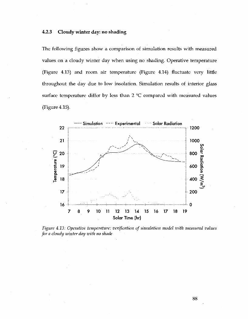
4.2.3 Cloudy winter day: no shading


values on a cloudy winter day when using no shading. Operative temperature

(Figure 4.13) and room air temperature (Figure 4.14) fluctuate very little

throughout the day due to low insolation. Simulation results of interior glass

surface temperature differ by less than 2 °C compared with measured values

(Figure 4.15).

Simulation Experimental Solar Radiation r 1200

7 8 9 10 11 12 13 14 15 16 17 18 19

Solar Time (hr)

Figure 4.13: Operative temperature: verification of simulation model with, measured values for a cloudy winter day with no shade

88

Experimental Simulation Solar Radiation 22 , r 1200

21

y 20

•2 19 a> a.

I 18

17

16

1000

800

o_ Q

a3

Q_

600 °. o 3

4 0 0 ?

200

7 8 9 10 11 12 13 14 15 16 17 18 19

Solar Time (hr)

Figure 4.14: Room air temperature: verification of simulation model with measured values

for a cloudy winter day with no shade

u 0

a> k.

-> n i_ 0) a. E 4i

20

19

18

17

16

16

14

13

12

11

10

•Experimental Simulation Solar Radiation 1200

1000 (A

o_ 800 |

o a. 600 I! o 3

400 ^ 3

200

0

7 8 9 10 11 12 13 14 15 16 17 18 19

Solar Time (hr)

Figure 4.15: Glass temperature: verification of simulation model with measured values for a

cloudy winter day with no shade

89

4.3 Description of thermal comfort model

A thermal comfort model was developed based on the transient two-node model

of Gagge et al. (1970) which considers the human body as composed of two

concentric thermal compartments: core and skin. This section describes the

numerical methods used for developing this simulation model (ASHRAE

Handbook of Fundamentals, 2005).

The rate of change of temperature of the core and skin is a function of its

heat storage and heat capacity of the body:

" cr _ ^cr ' ^D /A oc\

dt ( l " « S ) c ) " m , C ^

^ = Ssk'Au (4.36) dt ask-m-cph

where:

ask = fraction of body mass concentrated in skin compartment

m = body mass, kg

cp,b = specific heat capacity of body, J/ kg K

AD = DuBois surface area, m2

Tcr = temperature of core compartment, °C

Tsk = temperature of skin compartment, °C

t = time, s

The heat storage in each compartment can be expressed as:

90

Scr=M-W-(Cres-Eres)-Qcrsk (4.37)

Ssk=Qcrsk-(c + R + Esk) (4.38)

where Qcrsk is the heat transfer from the core to the skin by convection through

blood circulation and by conduction through the body tissue. It is calculated by:

QcrSk-(k+cpySKBF)(Tcr-Tsk) (4.39)

where k is the thermal conductance between the core and the skin, cv,b is the

specific heat of blood, and SKBF is the rate of blood flow to the skin

compartment.

During respiration, the body loses both sensible and latent heat by

convection and evaporation of heat and water vapour. These heat losses can be

determined by:

Cres = 0.0014M(34 - Ta) (4.40)

Eres = 0.0173M(5.87 - Pa) (4.42)

Convective and radiative heat losses from the outer surface of a clothed

body are related to their respective heat transfer coefficients:

C - / A ( T d - r . ) (4.42)

91

R = fA(Td-Tmrt) (4.43)

where:

fd = clothing area factor

hc = convective heat transfer coefficient, W/m2- °C

hr = linearized radiative heat transfer coefficient, W/m2- °C

Tci = temperature of clothing, °C

Ta = air temperature, °C

Tmrt = mean radiant temperature, °C

Several different equations can be used to determine the convective heat

transfer coefficient depending on the activity level of the person and the

condition of the surrounding air. For conditions typical of an office environment,

the following correlation can be used:

/zc=maxf8.3z;806, 3.l) (4.44)

The linearized radiative heat transfer coefficient (hr) is given by:

/zr = 4£o-(0.7) 273.2 + cl mrt (4.45)

where s is the average emissivity of clothing (0.95) and a is the Stefan-

Boltzmann constant.

92

Evaporative heat loss from the skin is a function of the amount of

moisture on the skin and the difference between the water vapour pressure at the

skin and in the surrounding air. It can be calculated by:

Esk=whe-(Psk-Pa) (4.46)

where w is the fraction of the skin surface covered by water, or skin wettedness,

he is the evaporative heat transfer coefficient, Psk is the saturated water vapour

pressure on the skin surface, and Pa is the partial pressure of water vapour at

ambient conditions. These can be evaluated by:

0 94-E w = 0.06 + rsw (4.47)

max

he = 16.5-im-hc (4.48)

where:

Ersw = rate of regulatory sweating, W/m 2

Emax - maximum rate of evaporative heat loss, W / m 2

im = moisture permeability of clothing

Skin temperatures and sweat rates required for comfort, tSk,req and ErSw,req

depend upon activity level (ASHRAE Handbook of Fundamentals, 2005):

?&,*„ = 35.7 - 0.0275(M - W) (4.49)

ErsW/rc=0A2(M-W-58.15) (4.50)

93

The mean body temperature (Tb) is therefore a weighted average of the

skin and core temperatures:

Tb=askTsk + 0--<Xsk)Tsk (4-51)

where ask is the fraction of body mass concentrated in the skin compartment and

is a function of the rate of blood flow from the core to the skin and the deviations

of skin and core temperature from their respective set-points:

n i 0.00028 . . „ . a ,*=0.1 + (4.52)

sk SKBF + 0.0011

SKBF. M + 20MVSTG. (4,53)

3600(1 + 0.5CSIGsk)

The rate of blood flow from the core to the skin is proportional with the

difference between the actual temperature and corresponding set-point value for

neutral condition:

Warm signal from the core:

0 T <T WSIGcr=

cr "" (4.54) cr cr,n cr cr,n

Cold signal from the core:

rjn rr-i r-j-i rri

/ - , r , T / - ! cr cr,n cr cr,n /A cc\

CSIGcr= (4.55) cr cr,n

Warm signal from the skin:

94

WSIGsk= ° 1**1** (4.56) 1sk 1sk,n lsk > is»r,n

Cold signal from the skin:

T T T T

C S I G ^ = 0 T >T ( 4 ' 5 7 )

Warm signal from the body:

0 T. =s T, WSIGb=

b b'n (4.58) 1b Lb,n 1b > 1b,n

where Tcrn = 36.80°C, Tbn = 33.70°C, andTb = 36.49°C.

Thermal sensation (TSENS) is defined in terms of the deviation of the

mean body temperature (Tb) from cold and hot set points. The set points

represent the lower (cold) and upper (hot) limit of the evaporation regulation

zone (TV and Tb,h , respectively) and are a function of the rate of internal heat

production:

TKc=^(M-W)+ 36.301 (4.59)

0 a.A'j TM=^(M-VV)+36.669 (4.60)

TSENS can then be calculated by:

95

TSENS =

0.4685(1,-T, J 3.995(Tb-TKc)/(Tbih-TbJ

3.995 + 0.4685(7;-T;,)

T b >TbrC

*-b,c ^ *-b ^ *-b,h

Tb,n<Tb

(4.61)

Thermal discomfort (DISC) is numerically equal to TSENS when Tb < Tb,c

and is related to skin wettedness when body temperature is regulated by

sweating. DISC is calculated by:

DISC = J

0.4685(Tb-Tb,c) Tb<TKc

4-7(Ersw-Ersw,req) (4.62)

^max ^rsw,req ^dif ^b,c ^ ^b

where Edif is the heat flow from evaporation of moisture diffused through the

skin.

The transient two-node thermal comfort model, like the building thermal

simulation model, requires a time-step based on numerical stability criteria. To

obtain numerical stability for the thermal comfort model, a time-step between 20

- 60 s is required (ASHRAE Standard 55, 2004); therefore, a 60 s time-step was

selected. Since the thermal data from the previous simulation was run on a five-

minute time-step it must be re-evaluated for the new 60 s time-step. This is done

by using the discrete Fourier Series and applying an inverse Fourier transform at

the 60 s time-step (Athienitis, 1998).

96

4.4 Comparison of thermal comfort model with measurements

It is generally a difficult process to validate or verify thermal comfort models

with measurements due to the assumptions used. Wissler (1988) suggests that a

model can be deemed acceptable if the predicted and measured values of mean

skin temperature agree within 2 °C. For comparison of thermal sensation,

however, values can present large differences not only due to limitations in the

mathematical model, but also due to experimental techniques used to assess the

perception of the indoor environment (Zmeureanu and Doramajian, 1992).

The results of the two-node comfort model are compared with

measurements taken by Grivel et al. (1989) The comfort model is also compared

with the results of a computer program developed by Gagge et al. (1986). In both

comparisons, mean radiant temperature is equal to air temperature.

Grivel et al. (1989) measured the skin temperature of six male and female

subjects in a climate chamber under cyclical ambient conditions. The ambient

temperature (air and mean radiant temperature) was kept constant at 28.8 °C for

one hour. Then, at a rate of 2 °C every eight minutes, it was decreased to 20.8 °C,

then increased to 34.8 °C, and then decreased again to 20.8 °C. The following

parameters were used in the simulation: body mass = 63.1 kg, body surface area

= 1.72 m2, clothing insulation = 0.1 clo, relative humidity = 50%, metabolic rate =

60 W/m2 , and air velocity = 0.2 m / s . The simulated results and measurements

are in good agreement, with differences smaller than 2 °C (Figure 4.16).

97

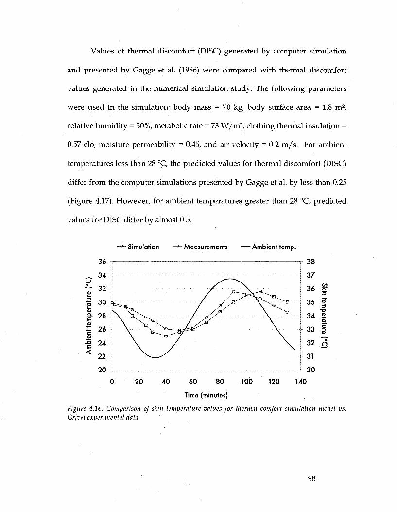
Values of thermal discomfort (DISC) generated by computer simulation

and presented by Gagge et al. (1986) were compared with thermal discomfort

values generated in the numerical simulation study. The following parameters

were used in the simulation: body mass = 70 kg, body surface area = 1.8 m2,

relative humidity = 50%, metabolic rate = 73 W/m2 , clothing thermal insulation =

0.57 clo, moisture permeability = 0.45, and air velocity = 0.2 m/s . For ambient

temperatures less than 28 °C, the predicted values for thermal discomfort (DISC)

differ from the computer simulations presented by Gagge et al. by less than 0.25

(Figure 4.17). However, for ambient temperatures greater than 28 °C, predicted

values for DISC differ by almost 0.5.

-Q- Simulation ~s~ Measurements Ambient temp.

0 20 40 60 80 100

Time (minutes)

120 140

Figure 4.16: Comparison of skin temperature values for thermal comfort simulation model vs. Grivel experimental data

98

- & _ Simulation -a _ Gagge model

2.5

2.0

1.5

1.0 U 52 0.5 a

0.0

-0.5

-1.0

-1.5 15 20 25 30 35

Ambient temperature (°C)

Figure 4.17: Comparison of thermal discomfort index for thermal comfort simulation model vs. Gagge computer model.

4.5 Parameters and assumptions

A parametric analysis of a typical office with glass facade in a south-facing

perimeter zone was completed in order to quantify the impact that different

glazing types and shading properties have on thermal comfort. This section

presents the parameters used and assumptions made for this analysis.

Climatic data

Representative days for winter conditions with clear and cloudy sky conditions

were chosen (Table 4.1) from the TMY data.

99

Table 4.1: Climatic data for representative days used in simulations

Sky condition

Clear Cloudy

Outdoor dry-bulb temperature ( °C)

Min Max

-22 -16 -19 -15

Maximum incident solar radiation (W/m2)

Beam Diffuse Total

735 310 1045 8 148 156

Outdoor temp, (clear day) Outdoor temp, (cloudy day) —*— Solar (clear day) —B— Solar (cloudy day)

0 1 2 0 o

8 9 10 11 12 13 14 15 16 17 18 19 20 Solar Time (hr)

Figure 4.18: Climatic data for representative days used in simulation

Room geometry

The geometry of the perimeter zone office is modeled as seven surfaces (ceiling,

floor, side walls, back wall, window, and facade wall containing the window),

with dimensions of 3.4 m x 3.0 m x 3.0 m (height x width x length). The window

is 2.4 m x 2.8 m (height x width) above the spandrel of height 0.8 m.

100

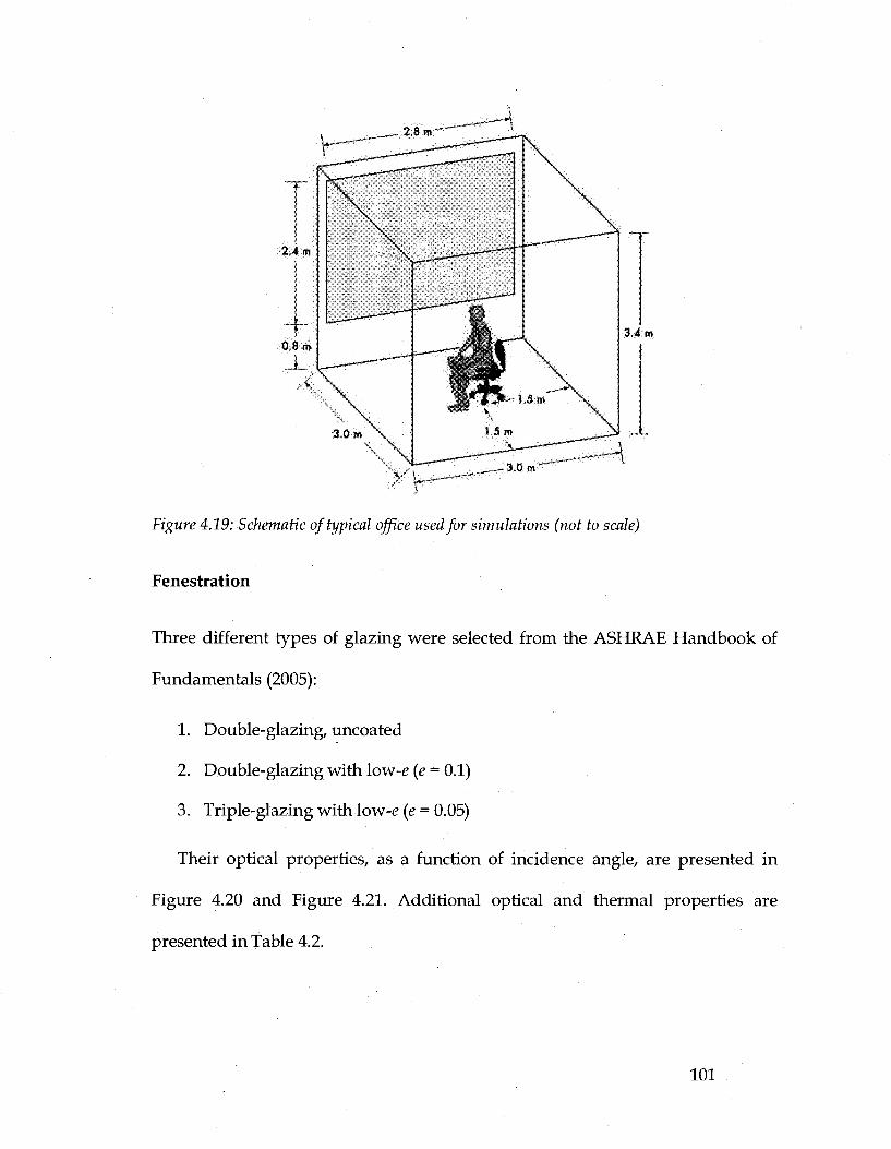
Figure 4.19: Schematic of typical office used for simulations (not to scale)

Fenestration

Three different types of glazing were selected from the ASHRAE Handbook of

Fundamentals (2005):

1. Double-glazing, uncoated

2. Double-glazing with low-e (e = 0.1)

3. Triple-glazing with low-e (e = 0.05)

Their optical properties, as a function of incidence angle, are presented in

Figure 4.20 and Figure 4.21. Additional optical and thermal properties are

presented in Table 4.2.

101

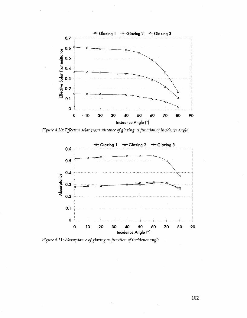
-s- Glazing 1 -* - Glazing 2 -®- Glazing 3

0 10 20 30 40 50 60 70 80 90

Incidence Angle (°)

Figure 4.20: Effective solar transmittance of glazing as function of incidence angle

0.6 Glazing 1 - * - Glazing 2 ~B~ Glazing 3

10 20 30 40 50 60 Incidence Angle (°)

Figure 4.21: Absorptance of glazing as function of incidence angle

70 80 90

Table 4.2: Properties of the three different glazing types used for parametric analysis (ASHRAE Handbook of Fundamentals, 2005)

Glazing

1 2 3

Visible Transmittance

0.78 0.53 0.55

SHGC

0.7 0.27 0.26

U-va

Center-of-glass

2.73 1.7

1.53

he (W/m2 °C)

Edge-of-glass

3.36 2.60 2.49

Total

3.51 2.63 2.43

The shading device type used for parametric analysis is a roller shade. Its

transmittance is kept at 5%. For parametric analysis its absorptance is varied

from 20% to 70%, and, hence, its reflectance is varied from 30% to 80%.

Building material properties

The floor, interior walls, and exterior fagade have an absorptance of 80%, 20%,

and 70%, respectively. Other thermal properties of the building materials are

presented in Table 4.3.

103

Table 4.3: Thermal properties of building materials used for simulation

F/oor Concrete Insulation

Exterior Wall Cladding Gypsum board Insulation

Interior walls Gypsum board Insulation

Ceil ing Gypsum board Concrete Insulation

Thickness (m)

0.2

0.1 0.02

0.02

0.02 0.2

Density (ka/m3)

2200

1800 800

800

800 2200

Specific heaf

(J/kg °Cj

1400

1005 750

750

750 1400

Thermal conductivity

(W/m °C)

1.7

1.3 0.16

0.16

0.16 1.7

Th resi (m2

ermaf isfance °C/W)

0.5

3

2

2

HVAC control

The HVAC system uses proportional-integral (PI) control for conditioning of the

air. It was determined that a proportional control constant of 500 W / °C and

integral control constant of 0.03 W / s would be necessary to adequately condition

the space. For heating, the set point temperature has a dead band of 1 °C.

Occupancy schedule

Internal gains from people (67 W) and lights/equipment (100 W) are modeled as

a heat source based on an occupancy schedule (8:00 - 20:00). Room air set point

temperature is also based on occupancy schedules with a daytime (6:00 - 22:00)

set point of 23 °C and nighttime (22:00 - 6:00) set point of 19 °C.

104

Other issues

Since it can take several time-steps for some of the parameters to reach

convergence in the building thermal simulation model, equivalent to several

simulation days, it would be unrealistic to assume that the occupant is "in the

space" for the time until convergence. This is because modeling the occupant as

being in the space during the night (while approaching convergence), when

conditions are outside of the comfort zone, would have an effect on the thermal

comfort conditions during the occupied hours. In other words, the effect of

discomfort caused by an occupant being modeled as being in the space during

the night would carry on into the occupied hours, thereby giving a false sense of

the actual comfort conditions that would occur in reality. Therefore, an

important assumption is made in relation to how thermal comfort is modeled for

an occupant while the building thermal simulation is running: during occupancy

off-hours (20:00 - 08:00) the occupant is modeled to be in a thermally neutral

state, i.e. room air and mean radiant temperature are forced to be 22 °C. Even

though the actual room air and mean radiant temperature in the space are not

these values, these parameters are used for the thermal comfort simulation

model so that an analysis of comfort during the occupied hours can start at a

reasonable value of DISC.

105

Indoor environment and occupant properties

The occupant is modeled as being seated in the center of the room facing parallel

to the fagade. The solar absorptance of clothing is divided into beam (aci,b) and

diffuse (aci,d) components, with aci,b = 0.8 (Blazejczyk et al., 1993) and aci,d = 0.5

(Lyons et al., 1999). Additional parameters related to the indoor environment

and occupant properties used for the simulation are shown in Table 4.4.

Table 4.4: Parameters of indoor environmental conditions and occupant properties used for the thermal comfort simulation

Metabolic

rate (met)

1.2

Body mass

(kg)

80

DuBois area

1.80

Air speed

(m/ i j

0.1

Relative humidity (%)

50

4.6 Results of simulation study

This section presents the most important results of the simulation study,

showing the impact that the three different glazing types and varying roller

shade properties have on occupant thermal comfort under clear and cloudy sky

conditions.

4.6.1 Clear winter day

The effect of solar radiation on thermal comfort has its greatest impact during

clear winter days. This is because a person has a larger projected area when the

sun is at lower altitude, thereby absorbing more solar radiation. For the same

reason, a vertical south-facing surface receives more incident solar radiation in

106

the winter months than in the summer months. Therefore, shading devices are

critical on clear winter days in order to avoid overheating due to the presence of

incident solar radiation. The properties of the shade, however, will determine the

degree to which comfort can be maintained.

The importance of taking solar radiation into account when modeling

thermal comfort in glazed perimeter zones can be seen in the results presented in

Figure 4.22. There is a 16 °C difference between the mean radiant temperature

due to the surrounding surfaces only and the mean radiant temperature due to

the surrounding surfaces and solar radiation with an unshaded double-glazed

uncoated window on a clear winter day.

- ° - MRT -*- MRT with solar Solar Radiation 1200

1 0 0 0 M o_ a

u 45 o "^ 40

i _

•H 35 1 o °° ! i - • A

8.30 j / ,<D 25 . S

' / T ^ 1 9

c 20 f ^ ° ^ o

^ 15 ' O '° ! cm c 10 1 o ! £ 5

8 9 10 11 12 13 14 15 16 17 18 19 20 Solar Time (hr)

Figure 4.22: MRT due to surrounding surfaces only and MRT due to surrounding surfaces and solar radiation with an unshaded double-glazed window on a clear winter day

When using no shading device on clear winter days, the solar-optical

properties of glazing have a pronounced effect on the mean radiant temperature

107

(Figure 4.24). During occupied hours (8:00 - 20:00), the predicted mean radiant

temperature ranged between 20 - 38 °C with glazing 1, 20 - 31.5 °C with glazing

2, and 20 - 25.5 °C with glazing 3. Room air temperature can reach as high as 27

°C with glazing 1 but only 23 °C with glazing 3 due to differences in

transmittance (Figure 4.25). The operative temperature ranged from 21 - 36.5 °C

with glazing 1, 21 - 31.5 °C with glazing 2, and 21 - 26 °C with glazing 3 (Figure

4.26). Radiant temperature asymmetry reaches above the maximum allowable 20

°C for all three glazing types (Figure 4.27). Discomfort reaches a maximum DISC

of +3.1 for glazing 1, +2.1 for glazing 2, and +0.9 for glazing 3 (Figure 4.28).

These results show how solar transmittance of glazing can affect the

thermal radiant environment and overall discomfort, especially with the lower

solar altitudes during winter.

~e~ Glazing 1 -*-Glazing 2 -H~ Glazing 3 Solar Radiation 3 0 T. , 200

8 9 10 11 12 13 14 15 16 17 18 19 20

Solar Time (hr)

Figure 4.23: Effect of glazing type on interior window surface temperature on a clear winter day

108

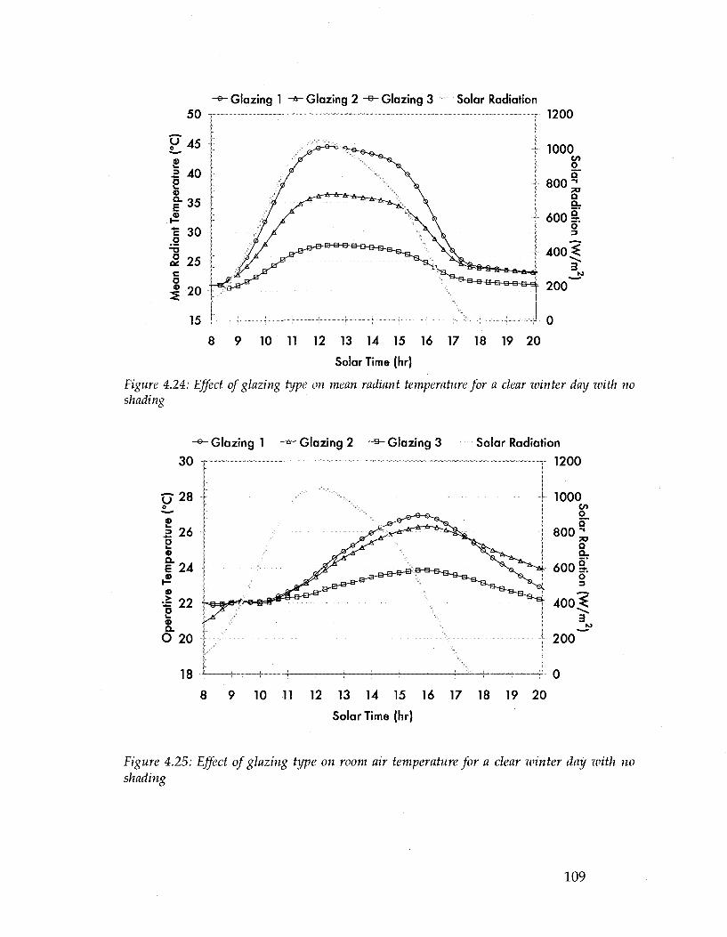
-®- Glazing 1 -*- Glazing 2 ~s~ Glazing 3 Solar Radiation

8 9 10 11 12 13 14 15 16 17 18 19 20

Solar Time (hr)

Figure 4.24: Effect of glazing type on mean radiant temperature for a clear winter day with no shading

-&- Glazing 1 -* - Glazing 2 ~s~ Glazing 3 Solar Radiation

30 r — - — - i- 1200

10 11 12 13 14 15 16 17 18 19 20

Solar Time (hr)

Figure 4.25: Effect of glazing type on room air temperature for a clear winter day with no shading

109

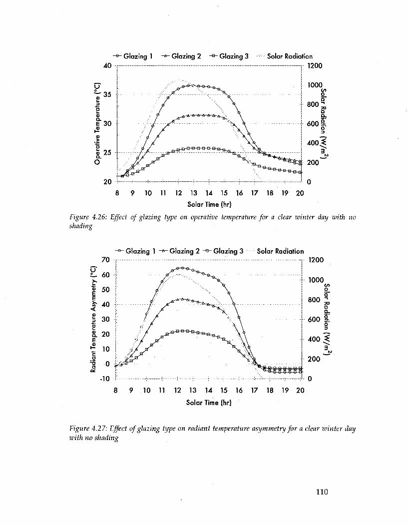
Glazing 1 -* - Glazing 2 -&- Glazing 3 Solar Radiation 1200

8 9 10 11 12 13 14 15 16 17 18 19 20

Solar Time (hr)

Figure 4.26: Effect of glazing type on operative temperature for a clear winter day with no shading

-&~ Glazing 1 -*-Glazing 2 -B-Glazing 3 Solar Radiation

8 9 10 11 12 13 14 15 16 17 18 19 20

Solar Time (hr)

Figure 4.27: Effect of glazing type on radiant temperature asymmetry for a clear winter day with no shading

110

Glazing 1 -*- Glazing 2 -a- Glazing 3 Solar Radiation 1200

8 9 10 11 12 13 14 15 16 U 18 19 20

Solar Time (hr)

Figure 4.28: Effect of glazing type on thermal discomfort for a clear winter day with no shading

When using a shading device, the thermal environment is highly dependent

upon the properties of the shade. An example of how shade temperature can

change with varying absorptance can be seen in Figure 4.29. With a shade

absorptance of 0.2 and 0.7, shade temperature with glazing 1 reaches a maximum

of 28 °C and 44.5 °C, respectively; with glazing 2, maximum shade temperature

reaches 26 °C and 37.5 °C, respectively; and with glazing 3, maximum shade

temperature reaches 24 °C and 29 °C, respectively (Figure 4.30).

I l l

Solar Radiation 1200

8 9 10 11 12 13 14 15 16 17 18 19 20

Solar Time (hr)

Figure 4.29: Effect of shade absorptance on shade temperature with glazing 2 (double-glazed, low-e)for a clear winter day

Glazing 1 - * - Glazing 2 - B - Glazing 3

45

40

u ^ 3 5

8 a> a. 30 E

25

20

0 0.1 0.2 0.3 0.4 0.5 0.6 0.7 0.8 Shade absorptance

Figure 4.30: Effect of shade absorptance on maximum shade temperature for a clear winter day

With a shade absorptance of 0.2 and 0.7, the simulated mean radiant

temperature with glazing 1 reaches a maximum of 23.5 °C and 29 °C,

112

respectively; with glazing 2, maximum mean radiant temperature reaches 23 °C

and 27 °C, respectively; and with glazing 3, maximum mean radiant temperature

reaches 22 °C and 23.5 °C, respectively (Figure 4.31).

-©- Glazing 1 -* - Glazing 2 -* - Glazing 3 30

U ^"28

s 2.26 E

1 24 TJ O

OS

I 22

20

0 0.1 0.2 0.3 0.4 0.5 0.6 0.7 0.8

Shade absorptance

Figure 4.31: Effect of shade absorptance on maximum mean radiant temperature for a clear winter day

With shade absorptance between 0.2 and 0.7, the maximum room air

temperature ranges from 24 - 30 °C for glazing 1; with glazing 2 it ranges from

23.5 - 28 °C; with glazing 3 it ranges from 23 - 25 °C (Figure 4.32).

With shade absorptance between 0.2 and 0.7, the maximum predicted

operative temperature with glazing 1 ranges from 23.5 - 29 °C; with glazing 2, it

ranges from 23 - 27 °C; and with glazing 3, it ranges from 22.5 °C and 24 °C,

respectively (Figure 4.33).

113

32

30

U" ^ " 2 8

i_

B <D

a. 26

Glazing 1 - * - Glazing 2 -JB~ Glazing 3

24

22

0.1 0.2 0.3 0.4 0.5 0.6 0.7 0.8

Shade absorptance

Figure 4.32: Effect of shade absorptance on maximum room air temperature for a clear winter day

-e~ Glazing 1 - * - Glazing 2 - B - Glazing 3

0 0.1 0.2 0.3 0.4 0.5 0.6 0.7 0.8

Shade absorptance

Figure 4.33: Effect of shade absorptance on maximum operative temperature for a clear winter day

When using a roller shade, the radiant temperature asymmetry is greatly

reduced as compared to using no shading. For all glazing types and shade

114

absorptances, the RTA due to a warm wall is kept below the upper limit of 23 °C

as recommended by ASHRAE Standard 55 (2004). The lowest radiant

temperature asymmetry is 3 °C for glazing 3 and a shade absorptance of 0.2; the

highest radiant temperature asymmetry is 18 °C for glazing 1 and a shade

absorptance of 0.7 (Figure 4.34).

-©-Glazing 1 Glazing 2 - Glazing 3

0 0.1 0.2 0.3 0.4 0.5 0.6 0.7 0.8

Shade absorptance

Figure 4.34: Effect of shade absorptance on maximum radiant temperature asymmetry for a clear winter day

The following three figures (Figure 4.35 - Figure 4.37) show the RTA at

different distances from the fagade for three different shade absorptances (0.2,

0.4, 0.7) for the three different glazing types. For each case the RTA is kept below

23 °C.

115

Shade absorptance: -©- 0.2 0.4

0.0 0.5 1.0 1.5 2.0

Distance from facade (m)

0.7

2.5 3.0

Figure 4.35: RTA as a function of distance from facade for three different shade absorptances using glazing 1

Shade absorptance: -®- 0.2 0.4

0.0 0.5 1.0 1.5 2.0


0.7

2.5 3.0

Figure 4.36: RTA as a function of distance from facade for three different shade absorptances using glazing 2

116

Shade absorptane: -e- 0.2 - H - 0.4 -*- 0.7 10

9

8

7

u °

s 5

& 4

3

2

1

0

0.0 0.5 1.0 1.5 2.0 2.5 3.0 Distance from facade (m)

Figure 4.37: RTA as a function of distance from fagade for three different shade absorptances using glazing 3

The maximum rating of discomfort on the DISC scale for glazing 1 ranges

from +0.5 to +1.9 for shade absorptance between 0.2 and 0.7. For glazing 2, the

maximum thermal discomfort ranges from +0.4 to +1.4. For glazing 3, the

maximum thermal discomfort ranges from +0.3 to +0.7 (Figure 4.38).

-°- Glazing 1 -*- Glazing 2 -B~ Glazing 3 2.0 T ~ - - - - - — -

1.5

u S2 1.0 a

0.5

0.0

0 0.1 0.2 0.3 0.4 0.5 0.6 0.7 0.8 Shade absorptance

Figure 4.38: Effect of shade absorptance on maximum thermal discomfort for a clear winter day

117

For glazing 1, the number of hours in a day outside the comfort zone

(DISC > +0.5) ranged from 0.5 hours to 9.5 hours, when using a shade with an

absorptance of 0.2 and 0.7, respectively. For glazing 2, it ranged from three hours

to just over nine hours when using a shade with an absorptance of 0.3 and 0.7,

respectively. For glazing 3, the DISC only exceeds +0.5 with shade absorptances

of 0.6 and 0.7, for three hours and over four hours, respectively (Figure 4.39).

o

i n IU 9

8

7

6

5

4

3

2

1 n u

Glazing 1

n 0.2 0.3

Glazing 2

0.4 O.i

Sh< 3d e abso rp tar

• Glazinc 13

- , J .

u ;'

- ,

r;

i i

i

i

i i

i 0.6 0.7

ice

Figure 4.39: Effect of shade absorptance on number of hours per day in discomfort zone for a clear winter day

Increasing shade absorptance decreases the heating load of the space for

all three glazing types (Figure 4.40). However, although glazing 3 has a slightly

higher insulating value than glazing 2, it has a lower solar transmittance.

Therefore, if using shading with an absorptance above 0.4 on clear winter days,

more heating is needed with glazing 3 due to lower solar gains.

118

-Q- Glazing 1 -*- Glazing 2 - e _ Glazing 3 6 -—-

l 4 -o c a | 3

Q O)

.S 2 a a>

X 1

0 •

0 0.1 0.2 0.3 0.4 0.5 0.6 0.7 0.8

Shade absorptance

Figure 4.40: Effect of shade absorptance on daily total heating demand for a clear winter day

4.6.2 Cloudy winter day

On overcast days in the winter, varying the shade absorptance has little effect on

the indoor environmental conditions due to low (or no) direct solar radiation.

Therefore, the comparison in this analysis only differentiates between the two

cases of using shading and not using shading. For all glazing types, using a

shading device increases the thermal performance of the faqade: the shading

device temperature is higher than that of the glazing interior surface and mean

radiant temperature is increased to be closer to room air temperature; therefore,

comfort conditions are improved. In addition, heating demand on cloudy winter

days decreases due to shading device use.

As expected, increasing the R-value of the window increases its interior

surface temperature to be closer to room air temperature (Figure 4.41). For all

119

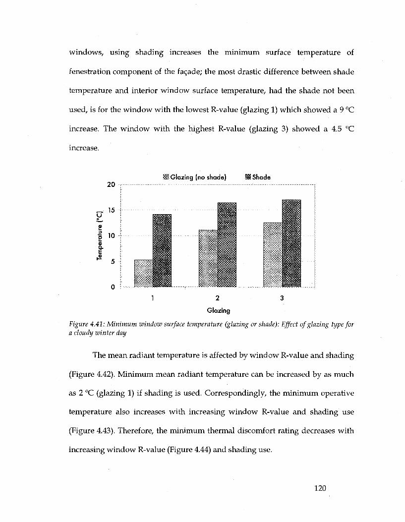
windows, using shading increases the minimum surface temperature of

fenestration component of the facade; the most drastic difference between shade

temperature and interior window surface temperature, had the shade not been

used, is for the window with the lowest R-value (glazing 1) which showed a 9 °C

increase. The window with the highest R-value (glazing 3) showed a 4.5 °C

increase.

...Glazing (no shade) MShade 20 T - \

1 10

1 2 3

Glazing

Figure 4.41: Minimum window surface temperature (glazing or shade): Effect of glazing type for a cloudy winter day

The mean radiant temperature is affected by window R-value and shading

(Figure 4.42). Minimum mean radiant temperature can be increased by as much

as 2 °C (glazing 1) if shading is used. Correspondingly, the minimum operative

temperature also increases with increasing window R-value and shading use

(Figure 4.43). Therefore, the minimum thermal discomfort rating decreases with

increasing window R-value (Figure 4.44) and shading use.

120

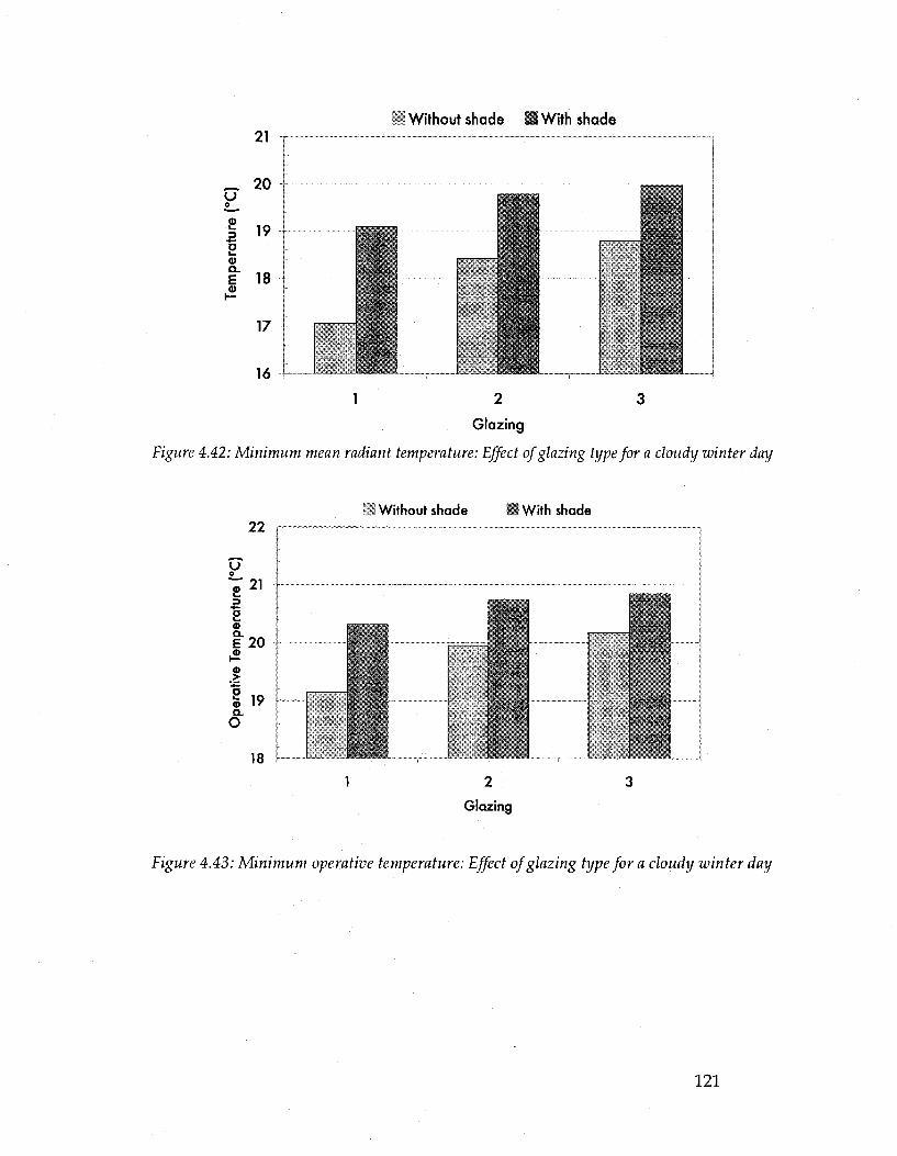
! Without shade SWith shade

E T

empe

ratu

re

20

19

18

17

" "

— . — •

•

•

i I

i 1 1 ! i j i

1 2 3

Glazing

Figure 4.42: Minimum mean radiant temperature: Effect of glazing type for a cloudy winter day

I Without shade S With shade 22

21 u o _

£

s « i"20

I § 19 a.

O

18

2

Glazing

Figure 4.43: Minimum operative temperature: Effect of glazing type for a cloudy winter day

121

u

n A ., u.u

-0.5

-1.0

1 K

Without shade

i

i

i

• With shade

-:

1 2 3

Glazing

Figure 4.44: Minimum thermal discomfort rating: Effect of glazing type for a cloudy winter day

Similarly, increasing the window's R-value decreases the heating energy

demand for the office and even more so if shading is used (Figure 4.45). A daily

heating demand of 16.3, 8.3, and 6.7 kWh is needed when using glazing 1, 2, and

3, respectively. If using a shading device, however, this demand can be reduced

by 42%, 41%, and 40%, respectively.

1 Without shade iWith shade 18

16

I" =£ 12 -u o 10 £ £ 8 o> .£ 6 o * A

0

1 2 3 Glazing number

Figure 4.45: Daily heating demand: Effect of glazing type for a cloudy winter day

122

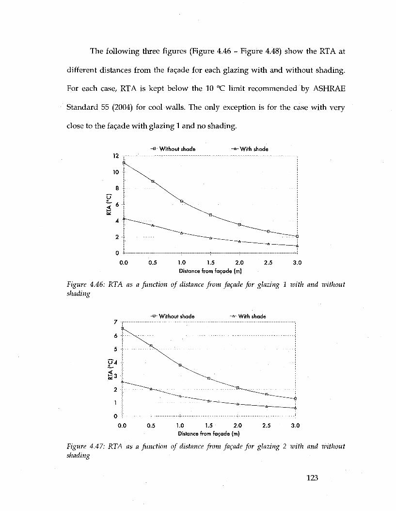
The following three figures (Figure 4.46 - Figure 4.48) show the RTA at

different distances from the fagade for each glazing with and without shading.

For each case, RTA is kept below the 10 °C limit recommended by ASHRAE

Standard 55 (2004) for cool walls. The only exception is for the case with very

close to the fagade with glazing 1 and no shading.

- Without shade With shade

0.0 0.5 1.0 1.5 2.0 Distance from facade (m)

2.5 3.0

Figure 4.46: RTA as a function of distance from facade for glazing 1 with and without shading

7

6

5

u4

S3-2

1

0

_B~ Without shade -*- With shade - —,

•

' 1

i


2.5 3.0

Figure 4.47: RTA as a Junction of distance from fagade for glazing 2 with and without shading

123

-a- Without shade ~*~ With shade 6

5

4 u" 0

I3

2

1

0

0.0 0.5 1.0 1.5 2.0 2.5 3.0 Distance from facade (m)

Figure 4.48: RTA as a Junction of distance from fagade for glazing 3 with and without shading

It should be noted that using a shade on a cloudy day is not typical since

occupants are more likely to take advantage of the view when the chance of glare

is minimal. Therefore, the results generated for the case with no shade would be

more indicative of reality. However, shading devices could be employed at night

to minimize heat loss through the fagade and increase comfort.

4.7 Further investigation using CFD

Although the finite-difference network model is adequate for performing

simulation of transient thermal environments, it handles air temperature as a

single node and air velocity as an input variable, and is, therefore, unable to

model the complex airflow and temperature stratifications that can occur within

the office. Thus, it cannot be used to predict local discomfort caused by

124

temperature stratification or air speed. For this reason, Computational Fluid

Dynamics (CFD) was employed for further analysis.

CFD is an established, state-of-the-art approach for quantitative prediction

and analysis of fluid flow and heat and mass transfer. For this study, the

commercial CFD software tool used was Airpak, which uses FLUENT as its

solver engine (Airpak 3.0 User's Guide, 2007). Airpak uses a finite-volume

formulation of governing differential equations used in CFD and can model basic

fluid flow, heat transfer (including radiation), turbulence, and contaminant

transport. These governing equations are adapted forms of the continuity

equation, the Navier-Stokes (or momentum) equations, and the energy

equations, based respectively on the fundamental principles of conservation of

mass, momentum, and energy. A detailed account of these equations can be

found in the literature.

4.7.1 Description of CFD model

A representative perimeter zone office was modeled with dimensions 3.4 m x 3.0

m x 3.0 m. The exterior wall has a window of dimensions 2.4 m x 2.8 m above a

spandrel of height 0.8 m. The part of the exterior fagade on both sides of the

window has a width and thickness of 0.2 m. Both the spandrel and exterior

fagade section have a thermal conductivity of 0.07 W/mK. The glazing is

modeled as having a U-value of 2 W/m 2 K (double-glazed, low-e).

125

An airflow analysis was completed for the case of a heated office under

winter conditions with the diffuser for supply heating at different locations on

the ceiling, with its center located 0.7 m, 1.1 m, and 1.5 m away from the

window.

Heating is supplied to the space through a diffuser at 30 °C and 1.5 m/s.

For boundary conditions in the model, outdoor air temperature is -20 °C and all

surfaces not exposed to outside (back wall, floor, ceiling, side walls) are assumed

to be adiabatic (no heat flux).

For an indoor air set-point temperature of 22 °C, the design heating load

was calculated to be:

Q —llJ .A .7 J .A \-(T —T\ y window window exterior exterior) \ R oj

'2 ™ W ^ J I - ^ W W ^ m2-°cj ^3m2-°CJ

= 662W

[22oC-(-20°c)l

The approximate size of the supply diffuser was then determined to be:

Q = 662W = m-cp-(rsupply -Treturn)

Q = 662W = Asupply • vsuppIy • p • cp • (rsupply - Treturn)

•'• Auppiy = 0.042m2 - 0.2m x 0.2m

Therefore, the diffuser was modeled to have an area of 0.2 m x 0.2 m. The

return vent was assumed to be 0.4 m x 0.4 m located 0.2 m from the back wall

126

(2.8 m from the window). The indoor zero-equation turbulence model was

selected for the flow regime since it was developed specifically for indoor airflow

simulations and is ideally suited for predicting indoor air flows that consider

natural convection, forced convection, and displacement ventilation (Airpak 3.0

User's Guide, 2007). Under-relaxation values for pressure (0.2) and momentum

(0.1) were selected based on convergence criteria for flow and energy. After

refining the grid size for the mesh, it was determined that a 0.095 m x 0.095 m

mesh would be sufficient to generate adequate results. A more refined mesh was

generated for components such as diffuser (0.02 m x 0.02 m) and return air vent

(0.04 m x 0.04 m). In total, the model contained 83,790 elements and 89,700 nodes.

/y* i

Figure 4.49: Model of perimeter zone office used for Airpak simulation (left); representation of mesh (right)

127

4.7.2 Results of CFD investigation

The resulting mean interior window surface temperature is 16 °C and the actual

heat loss through the fagade is calculated to be 554 W. Inner surfaces have a

mean temperature of about 23 °C. The calculated supply airflow rate is 5.80 L / s

(0.0687 kg/s), the mean temperature of supply air is 29 °C, and the mean return

air temperature is 26 °C. Therefore, the heat gain from the heating system is:

(^ = III Cp \1 guppjy — 1 r e t U m /

= 0 .0678^2-1005^—(34°C-26°C) s kg.K

= 552W

The variation in air speed as a function of distance from the window was

taken at three different heights from the floor, 0.1 m, 0.6 m, and 1.1 m,

corresponding to the heights of measurement of the ankle, chest, and head of a

seated occupant (ASHRAE Standard 55-2004). The following figures show the

differences in air speed at these heights for the diffuser at three different

distances from the window: 0.7 m (Figure 4.50), 1.1 m (Figure 4.51), and 1.5 m

(Figure 4.52).

128

h = 0.1m -«-h = 0.6m h = l . l m

U . J U

0.45

0.40

- . 0.35

£ 0.30

"I 0.25 j^O.20

< 0.15

0.10

0.05

0.00 •« p^^^~~e^'A S " ^ ^ — a ^ Z S " " " " ' ' -a B- _ / % ! !

-& U - J t r r l i


2.5 3.0

Figure 4.50: Variation in air speed at three different heights with diffuser 0.7 mfrom window (Tsupply = 30 °C; VsuWiy = 1.5 m/s)

0.0

-^-h = 0.1m -&-h = 0.6m h=1.1i

0.5

U . J U

0.45

0.40

^ 0.35

J . 0.30

1 0.25 » 0.20 L ,

< 0.15

0.10

0.05

0.00 i ^-^r^^^1-^—t^^^t^^^ 1.0 1.5 2.0


2.5 3.0

Figure 4.51: Variation in air speed at three different heights with diffuser 1.1 mfrom window (Tsuppiy = 30 "C; Vsuppiy = 1.5 m/s)

129

-a- h = 0.1 h = 0.6m -*-h=1.1r

0.0 0.5 1.0 1.5 2.0


2.5 3.0

Figure 4.52: Variation in air speed at three different heights with diffuser 1.5 mfrom window (Tsupply = 30"C; vsupply = 1.5 m/s)

Air Speed (m/s)

2.5

2H!

x 1.5

1-

0.5

O o o a i o ^>

p

I

v

0.5 1,5 2.5

1

0.9

0.8

0.7

0.6

0.5

0.4

0.3

0.2

0.1

0


Figure 4.53: Cross sectional contour plot of air speed with diffuser 0.7 mfrom window

130

2.5

I 1.5-

o.a

Air Speed (m/sj

/ ' I 0.6 P ' 0 ' " ^ •

. . o;i

«/._.

p

1

0.9

0.8

0.7

0.6

0.S

0.4

0.3

0.2

0.1

0

0.5 1 1.5 2


2.5

Figure 4.54: Cross sectional contour plot of air speed with diffuser 1.1 mfrom window

Air Speed {mis)

-'ill i'im :!'M

life ifilPi" .

' , / ! H

r^pcz^r^;-

'&> (''rJM¥'-X 1.5-j

o \ '0.6

°-r

a 50.5 -0.4

0.3

' f» \ r-» * \ '"> ' \ —' i i

^ '

0.1-

0.5

0.1.

0.5 1 1.5 2


2.5

Figure 4.55: Cross sectional contour plot of air speed with difusser 1.5 mfrom window

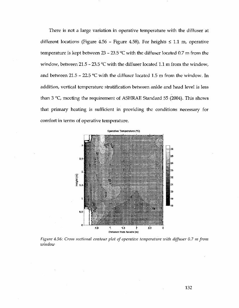
There is not a large variation in operative temperature with the diffuser at

different locations (Figure 4.56 - Figure 4.58). For heights < 1.1 m, operative

temperature is kept between 23 - 23.5 °C with the diffuser located 0.7 m from the

window, between 21.5 - 23.5 °C with the diffuser located 1.1 m from the window,

and between 21.5 - 22.5 °C with the diffuser located 1.5 m from the window. In

addition, vertical temperature stratification between ankle and head level is less

than 3 °C, meeting the requirement of ASHRAE Standard 55 (2004). This shows

that primary heating is sufficient in providing the conditions necessary for

comfort in terms of operative temperature.

Ui 2.5

24

x 1.841

0.5- I *

0.5

Operative Temperature f C)

mVi

8 0>

M

in

1 1.5 2 Distance from facade (m)

2.5

Figure 4.56: Cross sectional contour plot of operative temperature with diffuser 0.7 m from window

132

Operative Temperature ("CJ

a 2.5

2 - |

I 1.5-

•fi

0.5H BIBB

22S-~ 22

0.5 1 1.5

=3 5

22

2.5 Distance from facade (m)

|25

I B 24

1 123

22

21

20

19

18


Operative Temperature fC)

3-Bi

2.5

LK'v

0.5 X.

*«

* *

0.5

•22.6 . - 22"

.C<fc

1 1.5 2

Distance from facade fm)

' 2 a

•;2

26

— 25

24

23

22

21

20

19

18

2.5


133

The results from Airpak demonstrate the need for proper placement of the

diffuser in order to maintain comfort for occupants near the facade. Although

comfortable operative temperature is attained in each case, placing the diffuser

close to the window (0.7 m) would cause discomfort due to air speeds exceeding

0.45 m/s at the head level. The results also suggest that secondary perimeter

heating is not needed to mitigate cold downdraft or to increase operative

temperature near the fagade.

134

5 CONCLUSIONS AND RECOMMENDATIONS

5.1 Conclusions

This thesis has considered:

1. Thermal comfort in a perimeter zone office with glass fagade;

2. How exterior climate (air temperature and solar radiation) directly and

indirectly affects interior thermal conditions and thermal comfort; and

3. Shading device properties and glazing type and their use as a means to

improve thermal comfort.

An explicit finite-difference mathematical model was developed to analyze

the thermal conditions of highly glazed perimeter zones. A transient two-node

thermal comfort mathematical model was also developed to provide a prediction

of thermal comfort. The effect of shading properties on thermal comfort was

quantified.

Measurements were taken in an experimental perimeter zone using

thermocouples and an indoor climate analyzer to investigate the effect that the

exterior climate and shading devices have on the indoor thermal environment. It

was determined through the experimental study that shading devices can have a

positive impact on thermal comfort conditions in perimeter zones, preventing

135

overheating (minimizing operative temperature) on clear winter days and

increasing operative temperature on cloudy winter days. For both of these sky

conditions, the Venetian blinds only showed an improvement in comfort when

the slats were tilted at 45° or 90° (fully closed). A good agreement between the

measurements of the experimental study and simulation model was obtained.

Clear days in winter are the most complex conditions in terms maintaining

comfort and managing space conditioning. This is because the climate exhibits

contrasting thermal interactions: high incident solar radiation and cold air

temperature. Furthermore, comfort can be more difficult to manage due to low

solar altitude. This study has shown that not only the thermal resistance of

glazing, but also its solar transmittance, has a profound effect on thermal

comfort. Rooms that use glazing with low insulating value and high

transmittance exhibit the greatest fluctuations of the indoor thermal

environment. Rooms that use glazing with a higher insulating value and lower

transmittance create conditions which are more comfortable and less affected by

the exterior climate; however, there is a relationship between lower

transmittance of the glazing and increased demand of primary heating needed to

be supplied to the space due to decreased solar gains. It is evident that the

selection of fenestration components becomes a trade-off between energy,

thermal comfort, and lighting needs.

For cloudy winter days the indoor environmental conditions remain more

stable. For this case, indoor thermal conditions are dependent on the window

136

thermal transmittance. Even on very cold cloudy days, a highly insulating

window (i.e. triple glazed, low-e) can maintain comfort conditions. Regardless of

glazing type, using a roller shade can improve comfort conditions by decreasing

radiant temperature asymmetry and increasing operative temperature. For the

cases considered, perimeter heating could be eliminated when using a triple

glazed, low-e window or a double glazed, low-e window with roller shade.

However, it is not suggested to rely on the occupant using a shade on a cloudy

day since these climatic conditions provide an optimum scenario to take

advantage of glare-free daylighting and view.

Using CFD to analyze the airflow patterns in an office with double glazed

low-e windows on a cold cloudy day, it was determined that placing the diffuser

in the ceiling near the window (0.7 m) will cause discomfort near the window

due to elevated downdraft, with air speeds exceeding 0.45 m / s at head level. It

was also determined that secondary perimeter heating was not needed since the

primary heating could provide adequate thermal conditions by maintaining the

operative temperature in the comfort zone.

As noted in Chapter 4, it is generally a difficult process to validate or verify

thermal comfort models with measurements due to the assumptions used.

Furthermore, these assumptions (clothing insulation and absorptance, position in

the room, metabolic rates) are more complex in reality since they can vary from

person to person or even with respect to time. However, this work has been able

to show in general terms how thermal comfort in perimeter zones is affected by

137

glazing and roller shade properties and location of primary heating systems. It

was determined that with a high-quality building envelope (glazing U-value =

2.0 W/m 2 °C) and the diffuser for primary heating located away from the glazing

(1.1 m), cold air downdraft near the glazing would be reduced and operative

temperatures could be maintained within the comfort zone, thereby eliminating

the need for secondary perimeter heating.

5.2 Recommendations for future work

There are several possibilities for extension of current work. The work presented

in this thesis investigates whole-body thermal comfort. An investigation into the

impact of perimeter zones on local discomfort could be developed with a thermal

comfort simulation model for individual body segments.

Another possible extension would be to model the impact of Venetian

blinds on thermal comfort. It is currently difficult to model this since there is no

information in the literature on how to take complex surfaces into account for

mean radiant temperature; the process becomes even more difficult when

considering the varying amounts of solar radiation falling on the occupant due to

openings in the blinds. Therefore, it would be interesting to see if a model could

be developed based on experimental data.

Most importantly, however, would be the development of a model that

considers thermal comfort, visual comfort, daylighting, and energy management.

138

Since shading devices play an important role for all these parameters, control

strategies could be developed to optimize some or all of these criteria.

Furthermore, models that also consider or take into account occupant behaviour

would be advantageous since it is difficult to develop an automated control

strategy that predicts operating conditions when occupants have some control

over their work environment (i.e. shade position).

As with all thermal comfort prediction methods, which aim to provide

recommendations for building design in order to achieve comfort, there will be a

range of variability in the comfort conditions actually experienced by real people

under real conditions. Once a building is in use, it is important to consider

thermal comfort as part of the commissioning strategy by completing a post-

occupancy evaluation and adjusting any control strategy as necessary.

By considering comfort as a key element in building design from the

initial design stage to the occupancy stage, it can be ensured that new sustainable

high-performance and passive solar buildings are not only aesthetically pleasing

and energy-efficient, but also comfortable and enjoyable places to work and live.

139

REFERENCES

Architectural Energy Corporation (2004). Improving indoor environmental quality

and energy performance of California K-12 schools. No. D-2.2d - Final CFD

Analysis and Documentation Report.

ASHRAE. (2004). Standard 55 - Thermal environmental conditions for human

occupancy. Atlanta: American Society of Heating, Refrigerating, and Air-

Conditioning Engineers, Inc.

ASHRAE. (2005). Handbook of fundamentals. Atlanta: American Society of Heating,

Refrigerating, and Air-Conditioning Engineers, Inc.

Athienitis, A. K. (1998). Building thermal analysis (2nd ed.) Mathcad electronic

book, Mathsoft.

Athienitis, A. K. & Santamouris, M. (2002). Thermal analysis and design of passive

solar buildings. London: James and James.

Ayoub, J., Dignard-Bailey, L., & Filion, A. (2000). Photovoltaics for buildings:

Opportunities for Canada: A discussion paper. No. CEDRL-2000-72 (TR).

Varennes, Quebec: CANMET Energy Diversification Research Laboratory,

Natural Resources Canada.

140

Bauman, F., Andersson, B., Carroll, W., Kammerud, R. C , & Friedman, N. E.

(1983). Verification of BLAST by comparison with measurements of a solar-

dominated test cell and a thermally massive building. ASME Journal of Solar

Engineering, 105(2), 207-216.

Blazejczyk, K., Holmer, I., & Nilsson, H. (1998). Absorption of solar radiation by

an ellipsoid sensor simulated the human body. Journal of Physiological

Anthropology, 17(6), 267-273.

Blazejczyk, K., Nilsson, H., & Holmer, I. (1993). Solar heat load on man: Review

of different methods of estimation. International Journal of Biometeorology, 37,

125-132.

Cabanac, M. (1996). Pleasure and joy, and their role in human life. Proceedings of

Indoor Air '96.

Cannistraro, G., Franzitta, G., Giaconia, C., & Rizzo, G. (1992). Algorithms for the

calculation of the view factors between human body and rectangular

surfaces in parallelepiped environments. Energy and Buildings, 19(1), 51-60.

Carmody, J., Selkowitz, S., Lee, E. S., Arasteh, D., & Willmert, T. (2004). Window

systems for high-performance buildings (First ed.). New York: W.W. Norton &

Company, Inc.

141

Chaiyapinunt, S., Phueakphongsuriya, B., Mongkornsaksit, K., & Khomporn, N.

(2005). Performance rating of glass windows and glass windows with films

in aspect of thermal comfort and heat transmission. Energy and Buildings, 37,

725-738.

Chapman, K. S., & Sengupta, J. (2003). Development of a simplified methodology to

incorporate fenestration systems into occupant thermal comfort calculations. No.

1071. ASHRAE.

Clarke, J. A., Janak, M., & Ruyssevelt, P. (1998). Assessing the overall

performance of advanced glazing systems. Solar Energy, 63(4), 231-241.

Collins, M., Harrison, S. J., Nay lor, D., & Oosthuizen, P. H. (2002). Heat transfer

from an isothermal vertical surface with adjacent heated horizontal louvers:

Numerical analysis. Journal of Heat Transfer, 124:, 1072-1077.

Fang, Y., Eames, P. C , & Hyde, T. J. (2006) Electrochemical vacuum glazing may

improve thermal comfort in buildings. The International Society for Optical

Engineering.

Fanger, P. O. (1973). Thermal comfort. New York: McGraw-Hill Book Co.

Fanger, P. O., Melikov, A. K., Hanzawa, H., & Ring, J. (1988). Air turbulence and

sensation of draught. Energy and Buildings, 12, 21-29.

142

Fieber, A. (2005). Building integration of solar energy: A multifunctional

approach. (Licentiate Thesis, Department of Construction and Architecture,

Division of Energy and Building Design, Lund University, Sweden).

Fluent Inc. (2007). Airpak 3.0. User's Guide.

Gagge, A. P., Fobelets, A. P., & Berglund, L. G. (1986). A standard predictive

index and human response to the thermal environment. ASHRAE

Transactions, 92(2), 709-731.

Gagge, A. P., Stolwijk, J., & Nishi, Y. (1970). An effective temperature scale based

on a simple model of human physiological regulatory response. ASHRAE

Transactions,

Ge, H., & Fazio, P. (2004). Experimental investigations of cold drafts induced by

two different types of glazing panels in metal curtain walls. Building and

Environment, 39,115-125.

Grivel, F., Hoeft, A., & Candas, V. (1989). Body temperatures and thermal

perceptions during warm and cool periodic transients: Influence of clothing.

Proceedings of the Annual International Industrial Ergonomics and Safety

Conference, 217-224.

143

Hawthorne, W., & Reilly, M. S. (2000). The impact of glazing selection on

residential duct design and comfort. ASHRAE Transactions, 106(1).

Heiselberg, P., Overby, H., & Bjorn, E. (1995). Energy-efficient measures to avoid

downdraft from large glazed facades. ASHRAE Transactions, 101(2), 1127-

1135.

Hensen, J. L. M. (1990). Literature review on thermal comfort in transient

conditions. Building and Environment, 25(4), 309.

Hodder, S. G., & Parsons, K. (2007). The effects of solar radiation on thermal

comfort. International journal ofBiometeorology, 51(3), 233-250.

Huizenga, C , Zhang, H., Mattelaer, P., Yu, T., Arens, E., & Lyons, P. (2006).

Window performance for human thermal comfort. Final report to the National

Fenestration Rating Council. (Center for the Built Environment, University of

California, Berkeley).

Humphreys, M. A., Nicol, J. F., & McCartney, J. K. (2002). An analysis of some

subjective assessments of indoor air quality in five European countries.

Proceedings of the 9th International Conference on Indoor Air, Santa Cruz, USA.

86-91.

144

Hutcheon, N. B., & Handegord, G. O. P. (1995). Building science for a cold climate.

Institute for Research in Construction, National Research Council Canada.

KPMB Architects. Retrieved 11/01, 2007, from http://www.kpmb.com.

Kubaha, K., Fiala, D., Toftum, J., & Taki, A. H. (2004). Human projected area

factors for detailed direct and diffuse solar radiation analysis. International

Journal of Biometeorology, 49,113-129.

Kuhn, T. E., Biihler, C , & Platzer, W. J. (2000). Evaluation of overheating

protection with sun-shading systems. Solar Energy, 69(6), 59-74.

La Gennusa, M., Nucara, A., Rizzo, G., & Scaccianoce, G. (2005). The calculation

of the mean radiant temperature of a subject exposed to the solar radiation—

a generalised algorithm. Building and Environment, 40(3), 367-375.

Laforgue, P., Souyri, B., & Achard, G. (1997). Simulation of visual and thermal

comfort related to daylighting and solar radiation in office buildings. Paper

presented at the International Building Performance Simulation Association.

Larsson, U., & Moshfegh, B. (2002). Experimental investigation of downdraught

from well-insulated windows. Building and Environment, 37,1073-1082.

145

http://www.kpmb.com

Lyons, P., Arates, D., & Huizenga, C. (1999). Window performance for human

thermal comfort. ASHRAE Transactions, 73(2), 4.0-4.20.

Manz, H., & Frank, T. (2004). Analysis of thermal comfort near cold vertical

surfaces by means of computational fluid dynamics. Indoor and Built

Environment, 13,233-242.

Mclntyre, D. A. (1980). Indoor climate. Essex, England: Applied Science

Publishers, Ltd.

Nicol, F. (1993). Thermal comfort: A handbook of field studies toward an adaptive model.

London: University of East London.

Nicol, F. (2003). Thermal comfort. In M. Santamouris (Ed.), Solar thermal

technologies for buildings (pp. 164). London: James & James Ltd.

Nicol, F. (2004). Thermal comfort. Freiburg Solar Academy.

Nicol, J. F., & Humphreys, M. A. (2002). Adaptive thermal comfort and

sustainable thermal standards for buildings. Energy and Buildings, 34, 563-

572.

146

Park, C , Augenbroe, A., & Messadi, T. (2003). Daylighting optimization in smart

facade systems. Eight International IBPSA Conference, Eindhoven,

Netherlands.

Parsons, K. (2003). Human thermal environments: The effects of hot, moderate, and cold

environments on human health, comfort, and performance (2nd ed.). London:

Taylor & Francis.

Perez, R., Ineichen, P., Seals, R., Michalsky, J., & Stewart, R. (1990). Modeling

daylight availability and irradiance components from direct and global

irradiance. Solar Energy, 50(3), 235-245.

Poirazis, H. (2005). Single skin glazed office buildings: Energy use and indoor

climate simulations. (Licentiate Thesis, Department of Construction and

Architecture, Division of Energy and Building Design, Lund University,

Sweden).

Rizzo, G., Franzitta, G., & Cannistraro, G. (1991). Algorithms for the calculation

of the mean projected area factors of seated and standing persons. Energy and

Buildings, 17(3), 221-230.

147

Rueegg, T., Dorer, V., & Steinemann, U. (2001). Must cold air down draughts be

compensated using highly insulating windows? Energy and Buildings, 33,

489-493.

Shahid, H., & Naylor, D. (2005). Energy performance assessment of a window

with a horizontal Venetian blind. Energy and Buildings, 37, 836-843.

Shahid, H., & Naylor, D. (2005). Energy performance assessment of a window

with a horizontal Venetian blind. Energy and Buildings, 37, 836-843.

Tzempelikos, A., & Athienitis, A. K. (2007). The impact of shading design and

control on building cooling and lighting demand. Solar Energy, 81(3), 369-

382.

Tzempelikos, A. (2001). A methodology for detailed calculations of illuminance

levels and light dimming factors in a room with motorized blinds integrated

in an advanced window. (Master of Applied Science, Department of

Building, Civil, and Environmental Engineering, Concordia University).

Tzempelikos, A. and Athienitis, A.K. (2003). Modeling and evaluation of a

window with integrated motorized Venetian blinds. Proceedings of 3rd

International Solar Energy Society World Congress, Goteborg, Sweden, June

2003.

148

Tzempelikos, A. (2005). A methodology for integrating daylighting and thermal

analysis of buildings. (PhD, Department of Building, Civil, and

Environmental Engineering, Concordia University).

Tzempelikos, A., Athienitis, A. K., & Karava, P. (2007). Simulation of facade and

envelope design options for a new institutional building. Solar Energy, 81(9),

1088-1103.

U.S. Green Building Council (2007). Retrieved 07/01, 2007, from www.usgbc.org

Wissler, E. W. (1988). A review of human thermal models. In I. B. Mekjavic, E. W.

Banister & J. B. Morrison (Eds.), Environmental Ergonomics (pp. 267-285)

Taylor and Francis.

Zhang, H., Huizenga, C , Arens, E., & Wang, D. (2004). Thermal sensation and

comfort in transient non-uniform thermal environments. European Journal of

Applied Physiology, 92, 728-733.

Zmeureanu, R., & Doramajian, A. (1992). Thermally acceptable temperature

drifts can reduce the energy consumption for cooling in office buildings.

Building and Environment, 27(4), 469-481.

149

http://www.usgbc.org

Zmeureanu, R., Iliescu, S., & Jacob, Y. (2003). Radiation from cold or warm

windows: Computer model development and experimental validation.

Building and Environment, 38,427-434.

150

APPENDIX A: Perez irradiance model

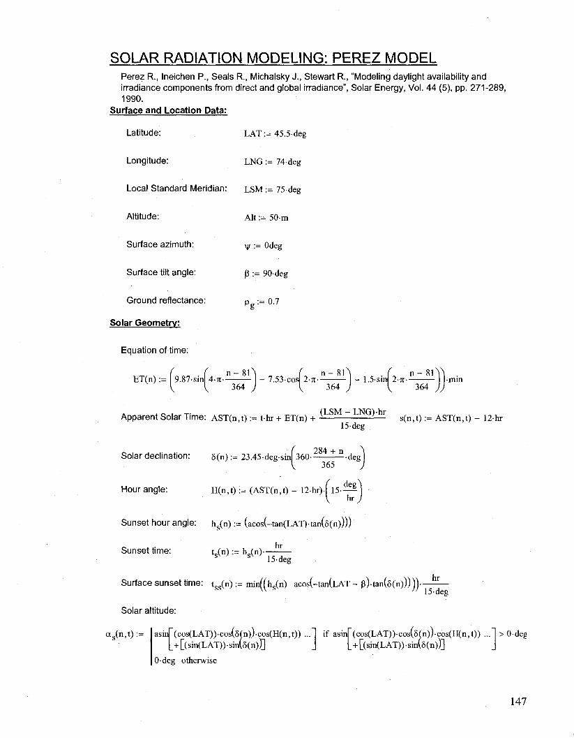
SOLAR RADIATION MODELING: PEREZ MODEL Perez R., Ineichen P., Seals R., Michalsky J., Stewart R., "Modeling daylight availability and irradiance components from direct and global irradiance", Solar Energy, Vol. 44 (5), pp. 271-289, 1990.

Surface and Location Data:

Latitude: LAT:= 45.5-deg

Longitude: LNG := 74-deg

Local Standard Meridian: LSM := 75-deg

Altitude: Alt := 50-m

Surface azimuth: y •= odeg

Surface tilt angle: p := 90-deg

Ground reflectance: p := 0.7

Solar Geometry:

Equation of time:

ET(n) := ( 9.87-sinf 4 - n — — J - 7.53-cosf 2n-^—^- J - 1.5-sinf 2 - j t - ^ - ^ - ) j-min

Apparent Solar Time: AST(n,t) := t-hr + ET(n) + ( L S M ~ L N G ) - r s ( n t ) : = A ST(n,t) - 12-hr

15deg

Solar declination: 5(n) := 23.45degsin[ 360 —-deg

Hour angle: H(n,t) := (AST(n.t) - 12hr)( 1 5 - ^

Sunset hour angle: hs(n) := (acos(-tan(LAT)tan(8(n))))

hr Sunset time: tc(n) := hc(n)

s s 15-deg

Surface sunset time: tss(n) := min((hs(n) acos(-tan(LAT - p)-tan(5(n)))))- hr

15-deg

Solar altitude:

a (n,t) := asin (cos(LAT))cos(8(n))cos(H(n,t)) ... if asin (cos(LAT))cos(8(n)j-cos(H(n,t)) _+[(sin(LAT))-sin(5(n))] J L+[(sin(LAT))sin(5(n))]

0-deg otherwise

Solar azimuth: <|>(n,t) := acos sin/a s(n,t)Vsin(LAT) - sin(5(n))

V coslas(n,t)Vcos(LAT)

H(n,t)

|H(n,t)|

Surface solar azimuth: ys(n,t) := (|)(n,t) - \\i

The angle of incidence, is: ee(n,t) := cos(as(n,t)ycos(|ys(n,t)| Vsin(p) + sin(as(n,t)Vcos(|3)

0(n,t) acos 86(n,t)+ |ee(n,t) |

(90deg) otherwise

if (l2hr - tss(n)) < th r < (l2hr + tss(n))

9(39, t)

deg

100

80

60

40 •K39,t) 2Q

deg Q

» # • • • a,(39,1) "20

deg -40

-60

-80

-100

Solar Time (hr)

Solar constant: I := 1367 W

m

Normal extraterrestrial solar radiation: Lx n(n) := L_-l 1 + 0.033-cosl ~-deg exnv ' • sc V 365

Hourly average global horizontal irradiance for Montreal:

Ih(n,t) = [lbn(n,t)(sin(a s(n,t))) + Idh(n,t)] W

Incident beam radiation on an inclined surface:

Ib(n,t):=(lb n(n,t)cos(e(n,t))). 2

m

Ibh(n>t) : = Ibn^'^^^s^11'1))

148

Perez diffuse irradiance model:

Diffuse radiation consists of three components:

1. Isotropic part, received uniformly from all the sky dome 2. Circumsolar diffuse, resulting from forward scattering of solar radiation and concentrated in the

part of the sky around the sun. 3. Horizon brightening, concentrated near the horizon, most pronounced in clear skies.

Anisotropic sky models have been produced initially by Hay & Davies (1980), and further developed by Reindl et al (1990). An anisotropy index is used to account for a portion of diffuse radiation which is treated as forward scattered. More recently, Perez et al (1988, 1990, 1993) produced more accurate models for treating the three parts of diffuse radiation on a tilted surface.

Horizon brightness coefficients:

ap(n,t) := max(o,cos(0(n,t))) bp(n,t) := max(cos(85-deg),sin(as(n,t)M

Relative optical air mass:

o p l • —1.253 sin(ac(n,t)) + 0.15-f a„(n,t) + 3.885

v s ' V 180-deg J Sky brightness:

W I dh( n - t ) -—

A(n,t) := mop t(n,t) - p -

Sky clearness:

e(n,t):=

W n ' t ) + W n - t ) - 6 / \3 + 5.535-10 (90-deg - a Jn , t ) )

Idh(n,t) V s I if Idh(n,t) > 0

1 + 5.535-10 -(90-deg - a s(n,t))

0 otherwise

Statistically derived irradiance coefficients for Perez model:

f n (n , t ) := -0.008 if s (n , t )< 1.065

0.130 if 1.065 <e(n , t )< 1.23

0.330 if 1.23 <e(n , t )< 1.5

0.568 if 1.5<s(n,t)< 1.95

0.873 if 1.95 <e(n , t )< 2.8

1.132 if 2 .8<s(n , t )<4.5

1.060 if 4 .5<s(n , t )<6.2

0.678 otherwise

f1 2(n,t): 0.588 if s(n,t) < 1.065

0.683 if 1.065 < s ( n , t ) < 1.23

0.487 if 1.23 <s(n, t ) < 1.5

0.187 if 1.5<£(n,t)< 1.95

-0.392 if 1.95 < s ( n , t ) < 2.8

-1.237 if 2 .8<s(n , t )<4.5

-1.600 if 4.5<s(n,t) < 6.2

-0.327 otherwise

f21(n,t):=

fl3(n,t):=

Brightness coefficients:

F|(n,t) := max

f22(n,t):= -0.060 if e(n,t) < 1.065

-0.019 if 1.065 <s (n , t )< 1.23

0.055 if 1.23<E(n,t)< 1.5

0.109 if 1.5<s(n,t)< 1.95

0.226 if 1.95 <E(n, t)< 2.8

0.288 if 2.8<E(n,t) < 4.5

0.264 if 4.5<£(n,t) < 6.2

0.156 otherwise

-0.062 if E(n,t) < 1.065 f23(n,t) :=

-0.151 if 1.065 <s (n , t )< 1.23

-0.221 if 1.23 <E(n,t) < 1.5

-0.295 if 1.5<£(n,t) < 1.95

-0.362 if 1.95 <£(n, t )<2.8

-0.412 if 2.8<E(n,t) < 4.5

-0.359 if 4.5<E(n,t)<6.2

-0.25 otherwise

0.072 if £(n,t) < 1.065

0.066 if 1.065 <£(n , t )< 1.23

-0.064 if 1.23 <£(n , t )< 1.5

-0.152 if 1.5<s(n,t)< 1.95

-0.462 if 1.95 <E(n, t )< 2.8

-0.823 if 2.8<E(n,t)<4.5

-1.127 if 4.5<E(n,t) <6.2

-1.377 otherwise

-0.022 if s(n,t) < 1.065

-0.029 if 1.065 <s(n, t ) < 1.23

-0.026 if 1.23 <s(n, t ) < 1.5

-0.014 if 1.5<e(n,t) < 1.95

-0.001 if 1.95 <E(n,t) <2.8

0.056 if 2.8<E(n,t) < 4.5

0.131 if 4.5<E(n,t)<6.2

0.251 otherwise

( 9 0 d e g - a (n,t)) 0 , f u (n , t ) + f12(n,t)-A(n,t) + n-- --f13(n,t)

180-deg

F2(n,t) := mad 0,f21(n,t) + f22(n,t)A(n,t) + n (90deg -a s (n , t ) )

180-deg f23(n,t)

Sky diffuse radiation on a tilted surface is calculated by

I s d(n, t ) :=Id h(n, t> ( 1 - F l ( n , t ) ) . ( 1 + co^)^ + F l ( n . t ) . ^ ^ + F 2 (n , t )W P ) bp(n,t)

_W 2

m

150

Ground-reflected radiation on a tilted surface:

L(n,t) := (lbh(n,t) + I d h (n , t ) ) P j 1 - cosl (p)" W

Total diffuse radiation on a tilted surface:

Id(n,t):= Isd(n,t) + Ig(n,t)

The total incident solar radiation on a tilted surface is equal to:

I(n,t) := Ib(n,t) + Isd(n,t) + Ig(n,t)

Components of diffuse solar radiation 400

a 3oo

a _ _ _

| I (39,t)-0.7 £ . . . . . 200 M Id(39,t)

100

1

_ — ™ _ _ ™ J L ™ .

1

: s • # * - # *

w * # * # • M *

/ • • ' " i

i i

• ^ S S i f c < * 3 , :

• \ '•

* \ * \ *• %s

« %'..

i ' * V . i _ _ .

1200

1000

10 15 20 t

Solar Time (hr)

Components of incident solar radiation

ition

(W

/m

Rad

i de

nt S

olar

1(39, t)

Ib(39,t)

Isd(39,t)

Ig(39,t)

800

600

400

200

25

# • * " * ***« t i l

10 12 14 16 IS 20 22 24

t Solar time (hr)

APPENDIX B: Room geometry and view factors

ROOM DIMENSIONS AND CALCULATION OF VIEW FACTORS

This file details the geometric dimensions of an office with one window. With this information, view factors between each surface can then be calculated to be used for radiation heat transfer analysis in the thermal simulation model.

Room Dimensions:

W := 3.2m ...width of room (along facade) D r m := 3m ...depth of room

H ^ := 3.0m ...height of room HL- := 2.0m ...height of window

EL„ := 0.8m ...height of spandrel (distance w„,:„ := \\f - 0.0001m ...width of window sp win rm

from window to floor) (equal to width of Window area (assume window is horizontally located at the middle of the wall):

room)

D w i n := H ^ - H - H ^ + 0.0001m ...distance from top of window to ceiling

D w i n = 0.2m

A w i n south : = Wwin'Hw m Awin s o u t h= 6.4 m ...window area

Wall net areas:

Asouth := V Wrm - Awinsouth Asouth = 3 ' 2 m - a r e a ° f W a " m i n u S w i n d o w

Awin WWR:=

south

^ m ' w r m WWR = 0.667 ...window-to-wall ratio

east' rm'^-m ''Svest • i east

Anorth : = Hrm-Wi rm Anorth = 9 6 m

A i- = W D ceiling rm rm floor • ceiling

V o 1 := Afloor-Hnn Vol = 28.8 m

Wall/window azimuth angles:

V south := 1 9 - 6 d e 8 Vnorth : = 199.6-deg

View Factors Between Internal Surfaces: The view factors for the room below are determined after first calculating the view factor between two rectangular finite surfaces inclined at 90 degrees to each other with one common edge:

J comm

h2

Define the following intermediate variables for calculating view factor from surface i to surface j :

wl w =

comm h =

h2

comm

2 2 A(h,w) := h + w

C(h):= 1 + h

B(w) := 1 + w

D(h,w):= 1 + ( h 2 + w2)

E(w) := w G(h) := h

View factor Fij from i to j :

w-atan| — + h-atan — II — ^/A(h,w)atan

+ 0.25-lrJ

Fij(w,h):=

V\/A(h,w)

E(w)D(h,w) AE(w) ( G(h)-D{h,w)f (h ) B(w)C(h)

B(w)A(h,w) C(h)A(h,w)

7t-W

D(h,w)

W rm

W win

D win

H wir

E win

H rm H_rm

W r m

Surf

East 2

ace 1

South 3

[2+3)

East 8

Floor 7

D rm

West 5

North 6

Ceiling 4

155

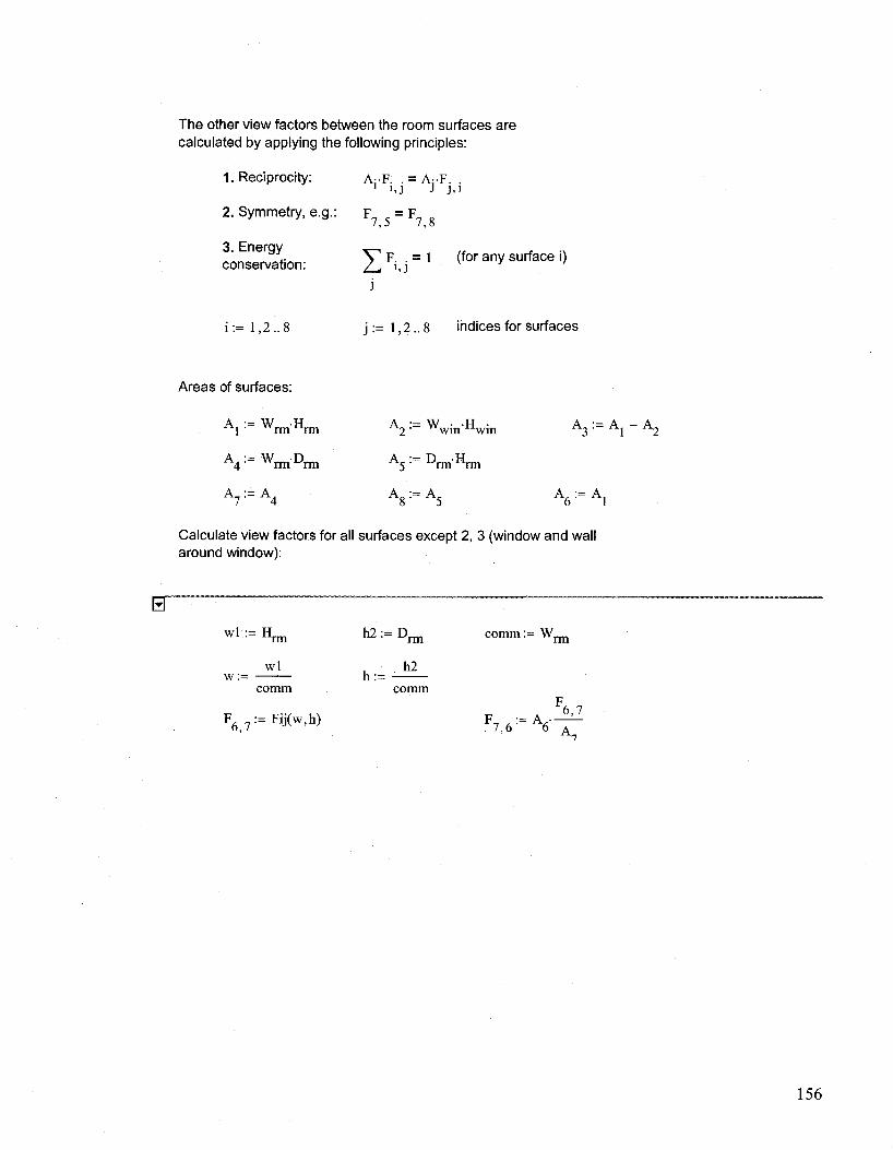
The other view factors between the room surfaces are calculated by applying the following principles:

1. Reciprocity: 1 i,j J J,i

2. Symmetry, e.g.: F ? 5 = F? g

.. V 1 F. . = 1 (for any surface i) conservation: ,/_, i,j v y '

j

i:= 1,2..8 j := 1,2.. 8 indices for surfaces

Areas of surfaces:

A ! := Wim-Hrm

A = W D 4 • vvrm ^rm

A r = A 4

A •= W • H • 2 ' win win

A5 : = D rm H rm

A 8 : = A5

A 3 : = V

A6 : = A l

" A 2

Calculate view factors for all surfaces except 2, 3 (window and wall around window):

0" w l : = H r m

wl w:=

comm

F 6 , 7 : = F i J( w ' h )

h 2 : = D n i l

h:= M

comm

comm := W_,

7,6 6 A

156

F *— F 6,4' 6,7

F 1 , 4 : = F 6 ; 7

F •— F 4,6" 7,6

F 1 , 7 : = F 6 , 7

F *— F 4,1 •"" 4,6

F 7 , 1 : = F 4 , 6

from symmetry

wl := W, rm

wl w:=

h2:= D,

h :=

rm c o m m : = H n n

h2

coiran

F 6 5 : = F iJ(w> h ) 5,6 6 A

6,5 F = F

6,8' 6,5

F *— F 8,6' 5,6

F = F F •= F 1,5' 6,8 5 , 1 ' 8,6

F = F 1,8' 6,8

F •= F 8 , 1 ' 8,6

w l : = H r m

wl w:=

comm

h2 := W,

h :=

rm

h2

comm

comm := D, rm

F 8 7 :=F i j (w ,h )

F 7 , 5 : = F 7 ,

8,7 F = A — F •= F

7 , 8 ' 8 A 5 , 7 ' 8,7 A 7

F 4 , 5 : = F 7 , « F •= F

5 , 4 ' 8,7

F •= F 8,4 ' 8,7

F •= F 4,8 7,i

a Determine the view factors for parallel opposite surfaces using the rule that:

VF. .=

F •= 1 - 2F - 2F 1,6' X Z f l , 8 Z r l , 4 F 6 , 1 : = F 1 , 6

F , •= 1 - 2-Fc . - 2 F , , 5,8 5,4 5,6

F 8 , 5 ' ' ~ F 5 , !

F 4 , 7 : = 1 - 2 - F 4 , 8 - 2 - F 4 , 6 F 7 , 4 : = F 4 , 7

Determine the view factor between the window and the floor. Note that the same equations may be used to determine the view factor between the window and all other surfaces except the back wall (6). F2 6 can be calculated from the fact that the sum of the view factors to all surfaces is equal to 1.

Calculation for view factors between window (surface 2) and floor (surface 7).

ET

H rm

W rm

rm

A b := W win D rm

A e : = W w i n H s p

•£*•£ • W „ , ^ * X 1 _ - . | ,

DIS :=

win *win W - W • rm win

Acl := Hwin-DIS

Aa := DISD, rm

Ac2 := HC„DIS

Aab := Dm-(D1S + Ww i n)

wl := D, rm

comm := W, win

wl w :=

Fb_2e:= Fij(w,h)

wl := D ^

comm := Ww i n

wl

h2 := Hwin + Hsp

h2

comm

...Ffrom Abto A2+Ae

h2 := H

h:=

sp

h2

comm

Fb 2e = 0.2

F b e := Fij(w,h)

wl := D, rm

Fb_e = 0.098

h2 :=H s p

158

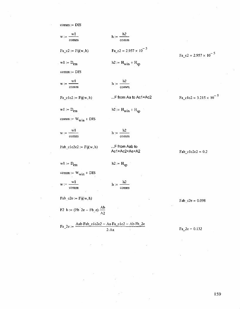
comm := DIS

wl w:=

comm

h2

comm

Fa_c2 := Fij(w,h)

wl := D m

comm:= DIS

Fa c2 = 2.957 x 10

h2 :- Hwin + Hsp

Fa c2 = 2.957 x 10 - 5

wl w:=

comm

h2

comm

Fa_clc2 := Fij(w,h) ...F from Aa to Ac1+Ac2 Fa clc2 = 3.215 x 10 - 5

wl := D, rm

comm := W,,.;„ + DIS Wil l

wl w :=

comm

h 2 : = H w i n + H! sp

h:= h2

Fab_clc2e2 := Fij(w,h) ...Ffrom Aab to Ac1+Ac2+Ae+A2 Fab clc2e2 = 0.2

wl := D, rm

comm := W,.„-„ + DIS Wil l

wl

comm

h2:= H,

h:=

sp

h2

comm

Fab_c2e := Fij(w, h)

F2_b := (Fb_2e - Fb_e)-Ab

A2

Fab c2e = 0.098

Fa 2e:= AabFab_clc2e2 - Aa-Fa_clc2 - Ab-Fb_2e

2-Aa Fa 2e= 0.132

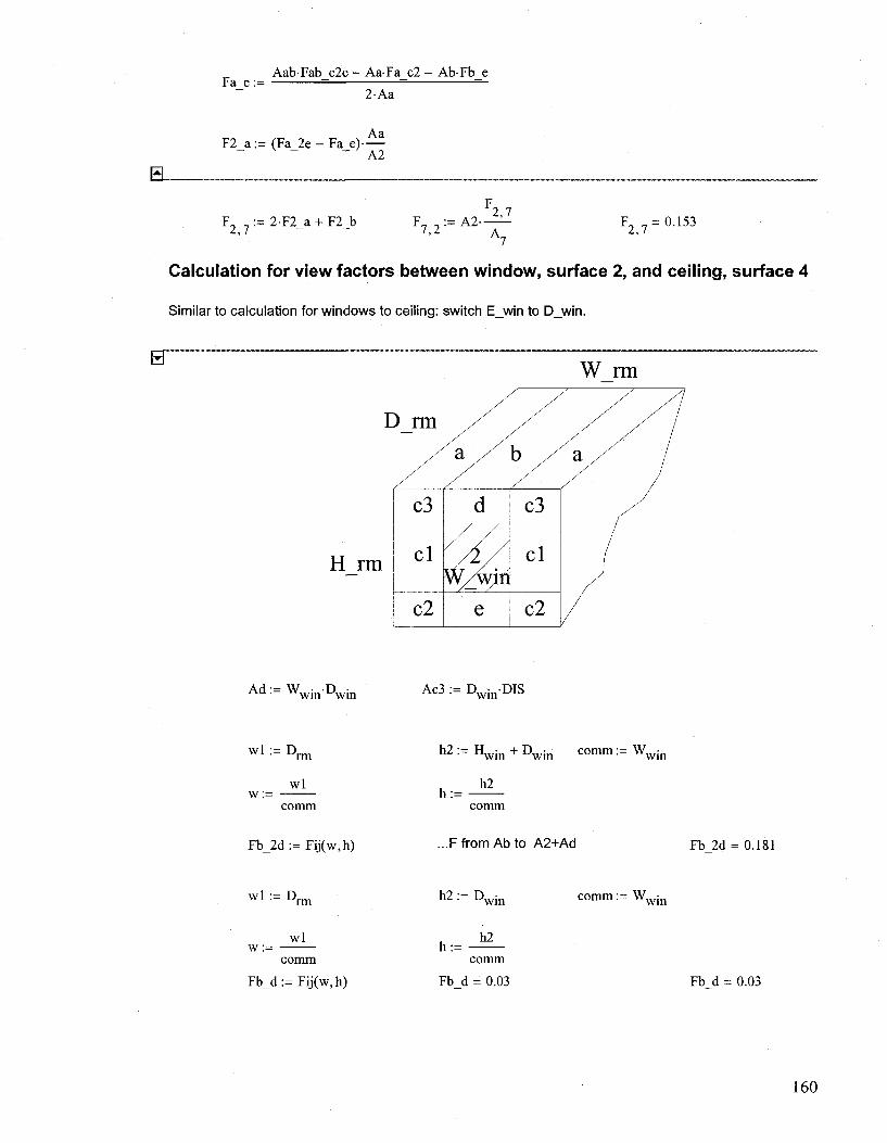
Fa e:= AabFab_c2e - AaFa_c2 - A b F b e

2-Aa

F2_a := (Fa_2e - Fa_e)-Aa

A2

F2 := 2-F2_a + F2_b 2,7

F7 :=A2 -7>2 A.

F2 ? = 0.153

Calculation for view factors between window, surface 2, and ceiling, surface 4

Similar to calculation for windows to ceiling: switch E_win to D_win.

ET W rm

H rm

Ad

wl

w::

Fb

•= W • D • • VYwin ^wrn

: = D rm

wl

comm

_2d := Fij(w: ,h)

Ac3 := Dwin-DIS

h2 := H w i n + D w J n comm := W w i n

h:= h2

comm

..FfromAbto A2+Ad Fb 2d = 0.181

wl := D,. h2 := D„ comm:= W„

wl w :=

comm

Fb_d:= Fij(w,h)

comm

Fb d = 0.03 Fb d = 0.03

wl := D, rm

h 2 : = D w i n comm := DIS

wl w :=

comm

Fa_c3 := Fij(w,h)

h:= h2

comm

Fa c3 = 2.597 x 10 - 5

wl := D, rm

wl w:

"^ : Hwin + Dwin

h:= h2

comm

comm := DIS

Fa_clc3 := Fij(w,h) ...Ffrom AatoAc1+Ac3 Fa clc3 = 3.177 x 10' - 5

wl := D rm

h 2 : - Hwin + Dwin comm := W w m + DIS

w:= wl

comm h:=

h2

Fab_2clc3d := Fij(w,h) ...F from Aab to Ac1+Ac2+Ad+A2

Fab 2clc3d = 0.181

wl := D, rm h ^ D w i n comm := W„„-„ + DIS

W i l l

wl

comm h:=

h2

comm

Fab_c3d := Fij(w,h) Fab c3d = 0.03

F2_b := (Fb_2d - Fbd) Ab

A2 Since Fa 2d = Fb clc2

Fa 2d := AabFab_2clc3d - AaFa_clc3 - Ab-Fb_2d

2-Aa Fa 2d = 0.117

Fa d:= AabFab_c3d - AaFa_c3 - Ab-Fb_d

2-Aa

F2 a:= (Fa 2d - Fa d) — " " A2

B

i „ . .— i- i ' i_a -r r i _ u «>2 A . 2 4 ~ 4 2 ~

Calculation for view factors between window, surface 2, and west/east wall, surface 518.

Similar to calculation for windows to floor.

0"

D rm

H rm

A d : = WwinDwin A e : = W win H sp A § := Dnn'Hwin A h : = D w i n D i rm A f : = H s p D r m

Acl := Hwin-DIS Ac2 := H -DIS Ac3 := Dwin-DIS Agh := Ag + Ah Agf := Ag + Af

wl := D, rm h2 := W w i n + DIS

comm := H„

wl w:=

comm h2

comm

Fg_2cl := Fij(w,h) ...FfromAgto A2+AC1 Fg_2cl = 0.174

wl := D,

w:=

rm

wl

comm

h2 := DIS

h2 h :

comm

comm := H. win

Fg_cl := Fij(w,h) Fe cl = 8.333 x 10 - 6

162

wl := D,.

w:= wl

coram

h2 := DIS

h2 h:=

comm

comm := D, win

Fh_c3 := Fij(w,h) Fh c3 = 8.327 x 10

wl := D, rm

wl

comm

h2 :=W w i n + DIS

h:= h2

comm

comm:= D win

Fh_dc3 := Fij(w,h) ___p from A h tQ A c 3 + A d

Fh dc3 = 0.041

wl := D,

w:=

rm

wl

comm

h 2 : = W w i n + DIS

h:= h2

comm:=Hw i n + D w i n

Fgh_clc3d2 := Fij(w,h) ...Ffrom Agh to Ac1+Ac3+Ad+A2 Fgh_clc3d2 = 0.181

wl := D,

w:=

rm

wl

comm

I := DIS

h2

comm

comm:=Hw i n + D w i n

Fgh_clc3 := Fij(w,h) Fgh_clc3 = 8.333 x 10 - 6

F2_g:=(Fg 2 c l - F g c l ) - ^ A2

Fh 2cl :=

Fh cl :=

Agh-Fgh

Agh-Fgh <

_clc3d2 • - AhFh_dc3 -

2-Ah

;lc3 - AhFh_c3 --Ag.

-Ag

Fg_

;-Fg_

cl

2c 1

2Ah

Fh 2cl = 0.106

Fh cl = 3.202 x 10

F2_h:= (Fh_2cl - Fh_cl) Ah A2

wl := D,.

wl w:=

Ff_c2 := Fij(w,h)

h2 := DIS

h2

comm := H, sp

h:= comm

Ff c2= 8.331 x 10 - 6

wl := D, rm

h2 :=W w i n + DIS comm:- H, sp

wl w:=

comm h:=

h2

comm

Ff_ec2:= Fij(w,h) F from Ah to Ac2+Ae Ff ec2 = 0.107

wl := D, rm

wl w:=

h2 :=W w i n + DIS

h:= h2

comm

comm := H ^ + H, sp

Fgf_clc2e2 := Fij(w,h) . . . F from Agf to Ac1+Ac2+Ae+A2

Fgf_clc2e2 = 0.199

wl := D,

w:=

rm

wl

comm

Fgf_clc2 := Fij(w,h)

h2 := DIS

h2 h:=

comm

comm:=Hw i n + H s p

Fgf_clc2 = 8.333 x 10 - 6

Ff 2cl:= Agf Fgf_clc2e2 - Af-Ff_ec2 - AgFg_2cl

2-Af Ff 2c 1 = 0.078

Ff cl := Agf-Fgf_clc2 - Af-Ff_c2 - A g F g c l

2Af Ff cl = 8.869 x 10 10

Af F2 f := (Ff 2c 1 - Ff cl)

A2

F2 f = 0.029 F2_g = 0.163

F, 7

2 5 := F2_h + F2_g + F2_f ¥§ 2 := A2-2,5

F2 h = 9.987 x 10

F •= F 2,8 - 2,5

- 3

F = F 8,2' 5,2

F 2 , 6 : l 2 'F2,5 F2,7 F2,4 F 6 , 2 : F 2 , 6 ' A

num:= 4 ,5 . . 8 F = F - F num,3 num, 1 num, 2

3, num ' num, 3 ^

F =

1

2

3

4

5

6

7

8

1

0

0

0

0.204

0.204

0.208

0.204

0.204

2

0

0

0

0.151

0.144

0.144

0.102

0.144

3

0

0

0

0.054

0.06

0.064

0.102

0.06

4

0.204

0.226

0.161

0

0.204

0.204

0.208

0.204

5

0.191

0.202

0.17

0.191

0

0.191

0.191

0.183

6

0.208

0.216

0.192

0.204

0.204

0

0.204

0.204

7

0.204

0.153

0.307

0.208

0.204

0.204

0

0.204

8

0.191

0.202

0.17

0.191

0.183

0.191

0.191

0

surf := 2 ,3 . .

suKij1 2-i Fi,surf Fsum

surf

VV

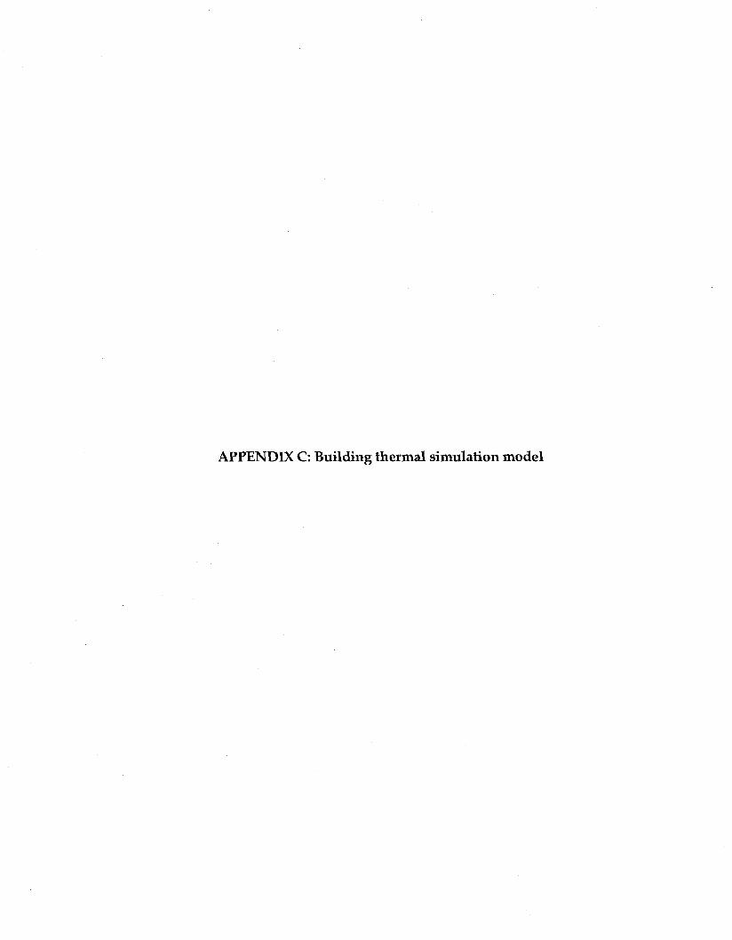
APPENDIX C: Building thermal simulation model

BUILDING THERMAL SIMULATION MODEL

i

This file is used for thermal analysis of the highly-glazed office space. The properties and dimensions of the surfaces and components are initially defined. Hourly values of incident solar radiation (beam and diffuse) are read from the Perez model. Representative days are selected for parametric analysis. Solar gains, thermal mass, heat transfer (convection, conduction, and radiation), and internal gains are modeled in detail. Glazing properties are modeled after data given in ASHRAE Handbook - Fundamentals, 2005 (Chapter 31, Fenestration). Therefore, the optical (transmittance, absorptance) and thermal properties of glazing were fitted to curves in Excel and used in Mathcad. Initial values of temperature and heat transfer coefficients are assumed; heat transfer coefficients are computed as a function of temperature at each time-step and the system of non-linear equations is solved explicitly in matrix form.

The results shown here are for an office with a south-facing facade in Montreal on a clear day in the winter. Shading with transmittance of 5% and absorptance 40% is used in conjunction with a double-glazed low-e window.

_8 watt d e g C ^ l < T : = 5 . 6 7 - 1 0

2 v* m K

Season and sky conditions:

The user can select the season (winter or summer) and sky conditions (clear or overcast)

season := 2 (summer = 1 or winter = 2) sky := 1 (clear = 1 or overcast = 2) 38 if season = 2 A sky = 2

39 if season = 2 A sky = 1

180 if season = 1 A sky = 1 Perez model

178 if season = 1 A sky = 2

...representative days selected from the

Roller shade properties:

shade := l ... set to 1 if shade is down, 0 if no shade is used

a • := 0.4 ...absorptance of shade % , := o.05 ...transmittance of shade

GLAZING PROPERTIES:

This file can six different types of glazing chosen from ASHRAE. Only three types were used in parametric analysis (1,4,6)

1 = ID #5b (uncoated double-glazing) 2 = ID#21a 3 = ID #21 d (low-e (e=0.1) double glazing) 4 = ID #25a (low e (e=0.05) double glazing) 5 = ID #40a 6 = ID #40d (low e (e=0.05) triple glazing)

ID := l ...selection of glazing type based on ID descriptions above.

166

Effective solar transmittance as a function of solar incidence angle:

t e(n, t) :=

f e ( n , t ) Y f 8 ( n , t ) Y 6(n,( -0.2152 +13.81 -278.54-—^-

^ deg J y deg J deg

+ 61350

100000

, 9 ( n , t ) f f e ( n , t ) V 6(n,t) -0.2206 +15.152 -315.26 +59408

if ID = 1

deg deg deg

100000

, 0(n , t )Y f 6 ( n , t ) Y 0(n,t) -0.13381 + 7.78624 - 151.47 + 4211 i

deg J \ deg J deg 100000

, ' e (n , t )Y fG(n, t )Y 0(n,t) -0.12211 +7.737 -163.1 +37169

deg J \ deg J deg

if ID = 2

if ID = 3

-0.0867-

100000

^9(n,t)Y r e ( n , t ) r 0(n,t) / ! +4.675-1 J \ - 122.02 + 28987

if ID = 4

deg deg deg

100000

; e ( n , t ) f f 9 ( n , t ) Y 9(n,t) -0.0407-1 1 + 1.6892-1 [ -36.026 +14981

if ID = 5

deg deg deg

100000 if ID = 6

W if l b ( n , t ) > 0 —

m

0 otherwise

Solar transmittance of first layer of glazing as a function of solar incidence angli

x(n,t)

-0.2668 ' 9 ( n , t ) x 3

deg + 17.956-

^Gfn.flV 9(n,t) 1 - 340.58- + 72542

deg deg

100000

, 0(11,0^ f e ( n , t ) Y 0(n,t) -0.2442 + 17.103- ' \ -331.26- +65519

deg deg deg

if ID = 1

if ID = 2

, 9(n,0 , -0.2271 I +16.165-

deg

100000

A 9(n , t )Y 0(n,t) 1 - 300.8- + 57552

V deg deg

100000

,' 0(n,t) \ 3 f 9 ( n , t ) Y 0(n,t) -0.151 +10.871- v ; -255.34- ' +41328

if ID = 3

deg deg deg

100000

l 0 ( n , t ) , \ 3 f 9 ( n , t ) V 0(n,t) -0.151 v +9.5141- -184.46- +45176

if ID = 4

deg deg deg

100000

, 8(n , t )Y f 0 ( n , t ) Y 9(n,t) -0.09951 +6.4989- \ -145.88- +33140

deg J \ deg j deg

if ID = 5

if ID = 6 100000

if l b ( n , t ) > 0 -W

0 otherwise

167

Diffuse transmittance and absorptance:

0.7 if ID = 1

0.65 if ID = 2

0.56 if ID = 3

0.35 if ID = 4

0.39 if ID = 5

0.39 if ID = 6

...diffuse transmittance of first glazing layer

r de : 0.51 if ID = 1

0.5 if ID = 2

0.35 if ID = 3

0.31 if ID = 4

0.23 if ID = 5

0.23 if ID = 6

...effective diffuse transmittance

' d i : 0.19 if ID = 1

0.2 if ID = 2

0.21 if ID = 3

0.26 if ID = 4

0.28 if ID = 5

0.35 if ID = 6

...diffuse absorptance of inner glazing layer

a d o : = 0.11 if ID = 1

0.27 if ID = 2

0.16 if ID = 3

0.04 if ID = 4

0.08 if ID = 5

0.03 if ID = 6

...diffuse absorptance of outer glazing layer

<dmid = 0 if ID = 1

0 if ID = 2

0 if ID = 3

0 if ID = 4

0.07 if ID = 5

0.14 if ID = 6

...diffuse absorptance of middle glazing layer

Solar transmittance of outer glazing as a function of solar incidence angle:

v3 /„,._ ^ \ 2

a 0 (n , t ) :=

-0.0013 ^ ( n . t ) ^ 4 ( 0 ( n , t ) y (Q(n,t)Y 6(n,t)

1 +0.1873 -7.2357 + 101.12 + 16949 deg deg deg deg

-0.0013 9(n , t )V f 0 ( n , t ) \ — ' - ^ - \ +0.1602 v ' \

deg J i deg J

100000

3 f 0 ( n , t ) Y 6(n,t) 5.9329 +88.986 + 19948

deg deg

-0.0013 e(n,t)

deg + 0.1873

9(n,t)

deg

100000

- 7.2357 G(n,t) 0(n,t)

+ 101.12 + 18949 deg J deg

100000

-0.0027 f0(n,t)

deg + 0.3629

^ e ( n , t ) x 3

deg 14.836

^ e ( n , t ) V 9(n,t) v ' ' ' +221.83 +23841 deg deg

100000

; 8 ( n , t ) ] 4 f 0 ( n , t ) V f 0 ( n , t ) V 6(n,t) -0.0037 +0.5178 -20.764 +281.7 +24809

if ID =

if ID = 2

if ID = 3

if ID = 4

deg deg deg

-0.0035 0(n,t)

deg + 0.4481

^ e ( n ; t ) x 3

100000

- 17.392

if ID = 5

^ ( n . o V 0(n,t) 1 + 242.39 + 33841 deg deg

100000 if ID = 6

0 otherwise

Solar transmittance of middle layer of glazing as a function of solar incident

o m i d ( n , t ) : = 0 if ID = 1

0 if ID = 2

0 if ID = 3

0 if ID = 4

, 6(n,t) , -0.0007 +0.0607

deg

' e ( n , t ) x 3

deg deg

, 0 ( n , t ) r 0(n,t) .6316 +36.844 +7001.9

deg

-0.0007 0(n,t)

deg + 0.057-

100000

^0 (n , t )V f 0 ( n , t ) V G(n,t) J] - 1.3312- +8.2881- +15002

if ID =

V deg deg deg

100000 if ID = 6

0 otherwise

169

Solar transmittance of inner layer of glazing as a function of solar incidence a

«j(n,t) :=

-0.0007 8(n,t)

deg + 0.0607

^0(n , t ) N 3 , 8(n,t) A 6(n,t)

-1.6316 +36.844 ' +11002 deg ) \ deg J deg

100000

, 6 ( n , t ) V ( '0(n,t) , \3 f -0.0009 +0.0983- -2.796-deg deg deg

8 (n , t )V 8(n,t) 1 +18.218- +7013.3

deg

100000

if ID = 1

if ID = 2

, 9(n,t) , -0.0022| | + 0.2739-

deg

/ 9 ( n , t ) A 3

deg deg

, 8(n,t) r 8(n,t) 10.396- —-^- + 138.93- + 15905

deg

100000 if ID = 3

0.0002 0(n,t)

deg J 0.04261 ( " ' { ) | +2.0696

deg

^0 (n , t )V 9(n,t) v ' I -27.171 v ' +4031.9 deg deg

, 9(n,t) , -0.00004| | +0.0103

deg

fe(n,t) V deg

100000

- 0.762 6(n,t) e(n,t)

+ 14.074 + 7013 deg ) deg

100000

, SCn.t)^ r 0 ( n , t ) V f 9 ( n , t ) V 8(n,t) -0.0002 +0.0142 -0.162 + 2.2007 +3010.4

deg deg deg

100000

0 otherwise

deg

if ID = 4

if ID = 5

if ID = 6

Conversion of outdoor variables for the day of interest:

T0( t) :=T0(n, t) yg(t) := ys(n,t) <x0(t):=<x0(n,t)

«i(t) :=aj(n,t)

a m i d ( t ) := a m i d ( n , t ) ag(t) := a s (n , t ) p( t ) :=p(n , t )

T(t):=T(n,t)

Te(t):=Te(n,t) e " ' ve'

U t ) := I_ (n , t )

TdpW^W"' 0

I_(t):=I_(t)-p.

Ib( t) :=Ib(n, t)

Id(t) := lsd(0 + lg(0

y ' ) : = I s d ( n , t )

I(t) := Ib(t) + Id(t)

p •= if(season = l,0.2,0.7) ...ground reflectance depends on season

170

1200

1000

1 at

ioi

arR

ad

1(0

%(0

WO

Ig(«)

800

600

400

200

Components of Solar Radiation T

t Solar Time (hr)

Optical Properties of Glazing T

Solar Time (hr)

171

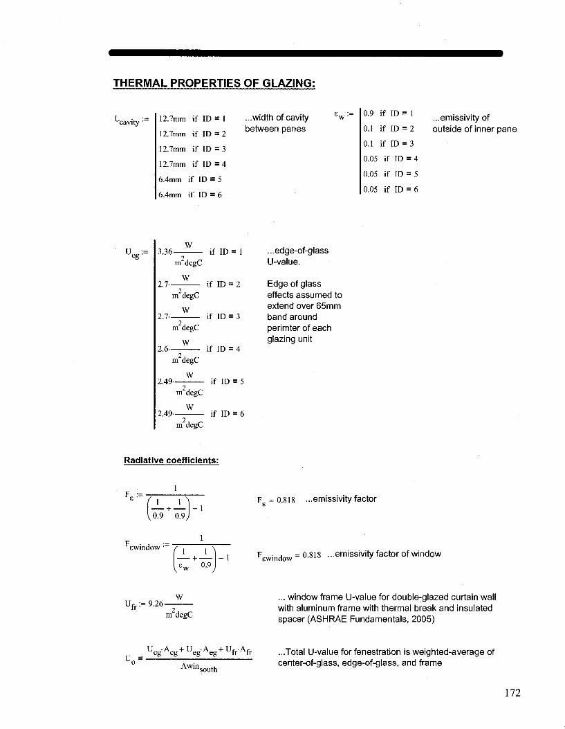
THERMAL PROPERTIES OF GLAZING:

"'cavity •" 12.7mm if ID = 1

12.7mm if ID = 2

12.7mm if ID = 3

12.7mm if ID = 4

6.4mm if ID = 5

6.4mm if ID = 6

...width of cavity between panes

s w : = 0.9 if ID = 1

0.1 if ID = 2

0.1 if ID = 3

0.05 if ID = 4

0.05 if ID = 5

0.05 if ID = 6

...emissivity of outside of inner pane

U eg : = 3.36-W

2.7-

m degC

W

if ID = 1

m degC

2.7-W

2.6-

m degC

W

m degC

if ID = 2

if ID = 3

if ID = 4

2.49-W

m degC

2.49-W

m degC

if ID = 5

if ID = 6

...edge-of-glass U-value.

Edge of glass effects assumed to extend over 65mm band around perimter of each glazing unit

Radiative coefficients:

F • -*V

1

^0.9 0.9 J

1 F

ewindow •

Ur_:=

f \ n l - w + °-9J

W 9.26

- 1

m degC

F =0.818 ...emissivity factor

F d =0.818 ...emissivity factor of window

... window frame U-value for double-glazed curtain wall with aluminum frame with thermal break and insulated spacer (ASHRAE Fundamentals, 2005)

_ ucg' Acg + ueg'Aeg + u f f Afr ...Total U-value for fenestration is weighted-average of o *„.;„ center-of-glass, edge-of-glass, and frame Awin, south

172

Acg := [ W w i n " 2-2(65mm)] . [H w i n - 2-2(65mm)]

Aeg := [ W win - 2(65mm)]-[Hw i n - 2(65mm)] - A c g

A f r : = (Wwin'Hwin) ~ A c g ~ Aeg

A c g = 5.115 m'

A e g = 0.625 rn

A f r = 0.659 m

W win H win = 6 - 4 m A c g + A e g + A f r = 6 - 4 m

Convection within cavity:

p •= 1 r a tnv '

T • win mean

Tg0ut + Tg in ...mean _ lOOdegC

- + 273 temperature of ^ m ~ ^ ~ inner and outer glazing

win mean

v . = win T.

0.002528.fTwin m e f m 1.5

PJ watt ...thermal conductivity of air in window

win mean + 200 mdegC

Rap = 2.737.(1+2-^ J - ^ 4 T - T •

gout gin P PI

cavity •P

^ mm J atm ...Rayleigh number

Nulp = 0.0605-(Rap) Nu2„ ! + •

0.104-(Rap) 0.293

1 + f6310V'36

Rap v l v apy

...Nusselt number

t i n hcglass = ~ - " i f ( N u l p > Nu2p,Nulp,Nu2p) ___ c o n v e c t i v e n e a t t r a n s f e r

P L, 'cavity coefficient within glazing cavity

OTHER PARAMETERS:

<xf:=0.8 ...absorptance of floor hCOnv :=3-5 ' W ... convective heat transfer

m degC coefficient between floor and basement

a := 0.7 ...absorptance of exterior wall awalls := °-2 " ' ' n t e n o r w a " s absorptance

Rinsglass:= 0.02lm2—— - insulated glazing unit

Temperature of adjacent rooms:

T a d j ^ := ifl season = X (26degC) if 1 < t < 6 v 22 < t < 24

(24degC) otherwise

(19degC) if 1 < t < 6 v 22 < t < 24

(23degC) otherwise

173

Exterior Heat Transfer Coefficients

hco = /hn2 + a (v )b ...outdoor conv. h.t. coeff. for glass

a and b are modifiers (2.5 and 0.75 on average, respectively).

v„ 24 if season = 2

10 otherwise .wind speed

hn = -

51 • JT„„-T.

1.382

go 'o ...Natural conv. coeff. for vertical surfaces

The radiative coeff. is calculated from the sky and ground temp, and their respective view factors.

h = 4-a-e Tm where Tm is the mean temp of the ro w outer glazing and outdoors:

T + T o go Tm = 2_ + 273

o~ co+ ro ...combined convective and radiative exterior heat transfer coefficient

Exterior heat transfer coeff. for outer glazing:

h o =

1.81 - / T „ „ - T , \2

go o 1.382

+ 2. ,5.(Vo)-]2 W m 2 K

• + 4-CTE,,

T + T o ^ "go > 13

+ 273 LV

•K J

Exterior heat transfer coeff. for wall surface:

hex = f'-81V T - T ex o

V 1.382 J

(

+ 1.Q " l . S l ^ T ^ - T ^ 2

L V 1.382 j 2.5 (v0)°-7 5]2 W »•«! j T e x - T o

m 2 K

+ 4.CT.£W. T + T ex o

+ 273 2 J

K

1.382

Interior Heat Transfer Coefficients

For convection_of interior surfaces, the following correlation is used:

i_

h • = 1.31AT3 where AT is the temp diff. between the surface and air temp.

For radiation_of interior surfaces, the following correlation is used:

_ CT(|[(T1+273)K]4-[(T2 + 273)K]1]-Fel2-F12-A1

'12 radiation between interior surfaces

Fi-T2

174

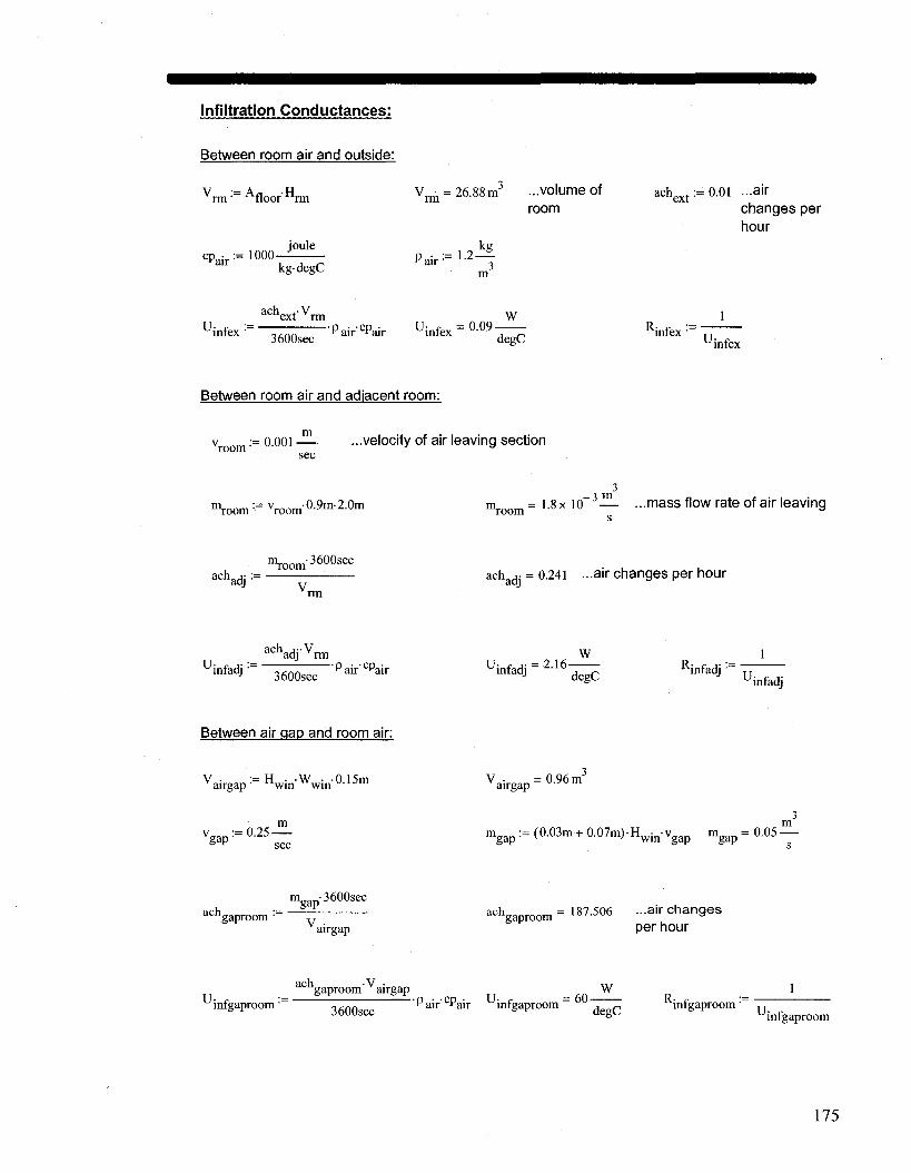
Infiltration Conductances:

Between room air and outside:

rm - floor rm

c p - :=1000. • ' a i r

joule

kg-degC

V rm = 26.88 m3 ...volume of room

. k g P a i r : = L 2 —

ache x t :=0.01 ...air changes per hour

a c h exf V rm W U infex : = , , Z -PaircPair Uinfex = ° - 0 9 - r

3600sec degC

R; infex ' U ; infex

Between room air and adjacent room:

v := o.OOl— ...velocity of air leaving section r o sec

m,.0„m := v,„„„,-0.9m-2.0m room • room

m n x J m = 1 - 8 x l ° _3 rn^

s ...mass flow rate of air leaving

ach "Voom 3 6 0 0 8 6 0

adj V.

achadj = 0.241 ...air changes per hour

U. infadj •

a c h ad j V rm

3600sec - P a i r ' ^ air Fair

Uinfadj = 2 J 6 W

degC R; infadj

U infadj

Between air gap and room air:

v - = H • W • 0I5m airgap • win "win "• ' J 1" Vairgap = ° - 9 6 m

vgap:=°-25-m g a p := (0.03m + 0.07m)-Hwin-vgap m g a p = 0.05-

ach m g a p ' 3 6 0 0 s e c

gaproom • v airgap

ach =187 506 ...air changes "^gaproom ° J " u a

per hour

U-ach V

gaproom airgap •Pa,VcPair

u = 60-W

R :, infgaproom • 3600sec pair' pair u infgaproom d c infgaproom U infgaproom

175

Between air gap and outside:

V - := H • W • -0.15m V - = 0.96m3 ach • := 0.01 ...air changes airsap win win aireap "• ; 'u l" at"gapext 3

per hour

rr achgapexfVairgap _ 3 W 1 u infgapext_

a , n n pair'cPair uinfgapext ~ i u x l u , n ^infgapext ~ T T

3600sec 8 P d e g C S P U i n f g a p e x t

Thermal Properties of Building Materials

Floor:

Concrete blocks: Lfloor:=0.2m kfloor:= 1.7 m- degC

kg joule

P f l o o r - 2 2 0 0 - i ^•-'m^^C m

Lfloor degC Rfloor := 7 " Rfloor = °-°X 2 —^T

kfloorAfloor W

2 p . . . . m degC insf degC lnsulat.on: Rinsf:=0.5 i L R i n s f :=- Rinsf = 0.052-2-

watt Rfloor w

Cfloor := ^oorPfloorAfloorLfloor Cfloor= 5 - 9 1 4 x ^ } - t h e r m a l t

capacitance of floor

Exterior (south) wall:

Brick:

Insulation:

Le x:=0.1-m p e x :

Lex e x ' k A . ex south

2 m

P — 3 l n s e x ' degCW

kg := 1 8 0 0 —

3 m

degC Re = 0.03—2-e W

^nsex ^ n s e x ' .

Asouth

cex joule

:= 1004.8-— kgdegC

kex := watt

= 1.3 m- degC

Cex := c exPex A sou th L e X Cex = 4 - 6 3 * ^ J - t h e r m a l capacitance of

exterior wall

176

East/west/north walls:

Gypsum board: W = ° - 0 2 m P e a s t : = 8 0 0 ~ T k e a s t - 0 - 1 6 ' kg

3

watt

m- degC ceast^=750-

joule

kgdegC

I •= I n •= n k •= k west' east H west" K east west' east

i-'««*-*t. •— t . north:~ Least p north : _ p east knorth :~ Keast K.,~-+u - ~ Ka cnorth • ceast

If considered as one: A ,I •= A ^u + A . + A t wall' -^northT ^west east

Awall = 25J6m

Lwall :~ Least+ Lwest+ Lnorth

^ a l l : -^ a l l

keast'Awall R w a l ^ 0 0 1 5

degC

W

Insulation: R- '— 2-inswall' degCW

R '= inswall'

inswall

A. wall

C wal l : _ ceast'p east'Awall'LWall Cwall = 9 - 2 7 4 * 1 0 J

Ceiling:

Gypsum board: Lceil := 0.02 P c e i l : = 8 0 o J T kcei l := 0- 1 6-

watt

m- degC cceil • 750-•

joule

kgdegC

Lceil \:eil • kceirAfloor R f loo r= 0 - 0 1 2

degC

W

Concrete blocks: L •• := 0.2m watt kg k c e i l : = L 7 — — P c e f l : = 2 2 0 0 - |

mdegC 3 cceil • 1400-

joule

kgdegC

bceil \;eil •

kceil'Afloor R c e i l = 0 - 0 1 2

degC

W

Insulation: R •= 2 insceil" degCW

R insceil'

insceil

A. wall

Cceil :~ cceirPceirAfloor'Lceil C c d l = 5.914x10" J

177

Air:

k a i r := 0.0257 watt

m- degC c a i r :=1005

joule

kgdegC 1.22

kg

Cair : _ cair'pair'(Afloor'Hrm) C • =3.296 x 10 J a l l

Since the room also contains furniture and other objects that can act as thermal mass, using the properties of air only is inadequate. Therefore, an estimate is made as to how the furniture can be lumped with the air capacitance ot make an "equivalent air capacitance" based on the ratio of furniture thermal capacitance (using wood as the material) to room air thermal capacitance:

cwood := 1 7 0 0 joule

kg-K Pwood •" 400-kg

Vol := 2.5m-1 m-0.75m = 1.875 m

Cwood :~ cwood'Pwood'(Vo1) Cwood=1-275xl° J

^wood

Cair = 38.686

...therefore, the equivalent room air capacitance should be a factor of about 40 greater than air capacitance alone.

O • = C • -40 ^air • ^air HU C • = 1.318 x 10 J air

View Factors:

Fsh_g := ' Fsky := °-5

Between floor and other surfaces:

floorceiling'_ 7>4

floor win _ 7,2

Ffloor_ceiling = 0 2 2 7

Ffloor win = 0 1 1 6

Ffloor south : = F7,3

F •= 1 — F —F —F floorwalls • floorsouth floorwin floor_ceiling

Ffl00r_south = 0 0 8 4

Ffloor walls = °-5 7 3

Between exterior (south) wall and other surfaces:

A floor south floor'

south floor south Fsouth floor" 0 3 1 4

Fsouth_ceiling :~ F3,4 Fsouth_ceiling ~ °'183

p ._ 1 p _ p south walls' south ceiling south floor p , „ - n 504 6 rsouth wa l l s - u : , w

Between window (or shade) and other surfaces:

Afloor p ._ p

win floor' A • floor win p . „ _ 0 174 Awin s o u t h - ^ w i n j l o o r - u ' 1 / 4

win_ceiling' 2,4 winceiling ~

p •— 1 F — F win walls • win ceiling win floor p . „ = o 6

- - - * w m -yvalls

Between ceiling and other surfaces:

A w i nsouth p ._ p p = 0 151

ceiling win ~ . win ceiling ceilingwin Afloor

F •= F ceiling floor' floor ceiling p ... „ _ n 997

- ceilingfloor

Asouth p ._ p ceiling south' . south ceiling p ... , = o 049

Afloor ~ rceilmg_south u ' w v

F *= 1 — F —F —F F = 0 57^ ceilingwalls' ceiling_win ceilingfloor ceilingsouth ceiling_walls "••"->

Between walls and other surfaces:

P . . C p f\ I AQ

walls win ~ . win walls walls w i n -

p ._ p p = 0 05 walls south' - . south walls walls south

walls floor' . floor walls walls floor u-^1 4

p l _ F F F F = 0 587 wallsceiling' wallswin walls_south walls_floor wallsceiling "•-'0/

AWlnsouth „

Awall

Asouth

Awall

Afloor

Awall

winwalls

southwalls

floorwalls

179

Selection of Simulation Time Step:

TS:= "floor "ceil ex

1 1 1 1 1 1 1 + + + hconvAfloor "^ +~ + ~Z + hconvAceiling 1 — + ~ + "

Kceil R,v„„™i Kceil & Kex R;„<™ Rfloor Rj n s f Rfloor

V 2 2 ceil Kinsceil cei l

2 2

ex insex

At := min(TS) dt:= 300sec ...simulation timestep

nda s : = 7day -number of days to run simulation

p:= 1,2.. "days

days 3 = 2.016x10

dt ...number of timesteps

dt

Transformation from hourly simulation to selected time-step:

Fourier transform:

2-7t(nn- 1) nn:= 1,2.. 7 j : • = ^

24- hr coco := 2 .0-

24

T0(t) := -17 - 2-cos| coco-t+ 5.2— |-degC if season = 2 A sky = 2

- 1 9 - 3-cos GH0-t+ 5.2— -degC if season = 2 A sky = 1

( A 28 - 3-cos co«)t+ 5.2— degC if season = 1 A sky = 1

( A 24 - 2-cos <oa)-t+ 5.2— degC if season = 1 A sky = 2

...outdoor temperature for representative days

T o »

-20

Solar time (hr)

180

" o : = E T < > ( t ) ' ~ ^ nn - i -^ 24

TT dP„ ?Z¥

ex^-jro^-thr)

24

n„n:=]Ti(t) exp(-j(Bnnthr)

24 n b : = V i b ( t ) nn t—i

exj^-j-cflnn-t-hr)

24

Hd : = V l d ( t ) nn -t—'

exp(-j(onnt-hr)

24 • 5 > exp(-J0)nnthr)

24

aa: := nn Xai(t)

exp{-jo)nnthr)

24 T^ exp(-JQ)nnthr)

24

*0 ^y^w-n n •*—J

exp(-jwnnthr)

24 Zexp(-jO)nnthr)

x(t) 1 '-24

YYS : = ^ y s ( t ) exp(-jconn-thr)

24 :=£«s(t)-

exp(-j(Bnnthr)

24

î-IW) exj^-jOnn-t-hr)

24 a amid : = y a m i d ( t )

nn •*—'

exp(-jo)nnt-hr)

24

tp := pdt ...times at which simulation will be performed

Generation of data for each time step (back in time domain):

nl :=2,3.. 7

T0 := TT„ P

o1

+ 2 f Z R e ( T r on l '

e x ^ m n r ^ Inl

Ib :=if| \ W

I lbl + 2 ' E ReTIIbnl-eXP(j<anrtp)) J > ° ~ ' H b + 2 ' E Re(IIbni

eXP( j-<Dnl tp) Inl " J V nl

\ W ^ 0

Id := ifl IId +2-l^

nl

ReTlIdêx^jm^tp)^ > 0 — ,IId + 2-|^T ReAljêx^jcOnrtp)

J m Inl

x 0 2 m

J

Ip •= ifl

nl

w " ' + 2 f Z ! ^ " n r ^ J ^ n r t p ) ) J > ° — ' I ] l + 2 j ^ R e ( n n i e x p ( j o ) n r t p ) ) j , 0 —

nl

W

<x0 :=ifl P

a a 0 + 2 j V R c / a a 0 -ex^jconjtp)^

Ul > 0 , a a + 2-

1 V R e ^ a a Q e x p ^ a ) ^ - ^

. nl

oij := if P

a a j +2-(\^ Refaa- exp(jG)ni-tpn > 0 , a a j + 2 | \ ^ R e | a a j exp(jcon|-tpJ

Ul " J Ul ,0

J J

a mid p : = if ""mid, + 2 | X ^ " m i d ^ - ^ K j ^ n r t p ) ) ) > ^ " " m i d , + 2 | X R e ( a a m i d n l

e x P ( j M n r t p F )

Ui ) Ui ,0

J J

T^ := ifl TT„ + 2 ' l S R e f T T e -exp(j'(8nr1p)')| > °'TTe + 2 " f y ] R € f T T e •exp(i-0)nrtp)")|'0

Tp := if " i + 2 | V Re(rrnrexp(j-G)nrtp))| > O.TTJ + 2 [ V Re(TTnlexp(jo)nr1p))

Ul J Ul ,0

J J

a s :=if| P

n s + 2 ' ( V R e 6 r s •exp(j-o)nrtp)'

v\

V Re/'aa s • exp( j - co n l • tp)^ a a . + 2- > 0 ,aa„ +2 ' s l

Tadjp : = " a d j , + 2 | X R ^ a d J n l

e x P O ' r o n r t p )

Ul

'dp : = TTdPl + 2 | 2 R^TTdp^^J^nrV)

Ui

V R e ^ a a s •exp(ja)n,tp)N\

nl

^ 0

J J

Tsky : - ( T o P V B

0.8 + -'dp

P 250 J

Internal gains:

Q i n t := if(8-3600sec < mod(pdt, 24-3600sec) < 20-3600sec, 167W,0W) ...internal gains from equipment P (100 W) and person (67 W) during

occupied hours

CONTROLS:

Set-point temperatures vary between summer and winter and between night and day. Conditioning of the air is modeled with proportional-integral (PI) control.

182

T := iff season = 1, 24degC if 8-3600sec < mod(p-dt,24-3600sec) < 20-3600sec

26degC otherwise

23degC if 8-3600sec < mod(

19degC otherwise

v= (600W) if season = 1

(500W) if season = 2 ...proportional control constant Kj := 0.03

W

sec ...integral control

startt :=

n d a y s - l d a y

dt startt = 1.728 x 10 endt :=

"days

dt endt = 2.016 x 10

offset := OdegC

sPn

'adL

25

24

23

22

21

20

19

18

17

16

15. 120 125 130 135 140 150 155 160 165 170 145

dt P'hr

When using PI control, control of the air conditioning is based on an integration of the deviation of actual air temperatures at previous time steps from the desired set-point temperature. Integral control is based on deviations of air temperature from set-point temperatures at previous time-steps. Since the set-point temperature changes from day to night, the PI control must only take into account deviations of previous values of air temperature from the set-point (not necessarily at the present time-step). For this reason, the time-step "counter" must be "reset" at each change of set-point temperature. The following lines outline the modeling needed in order to take this into account:

ppday := 24hr

dt ( P "1 pinitiaL := flooij ppday VPPdayJ

p_in_daytimep := pinitiaL + 8 hr

dt penddaytimep := pinitiaL + 20

hr

dt

pKIp:= 1 if p < hr

dt

p_in_daytimep if 8-3600sec < mod(p-dt,24-3600sec) < 20- 3600- sec

otherwise

p_end_daytimep if mod(pdt,24-3600sec) > 20-hr

(penddaytimep - ppday J if mod(pdt, 24-3600sec) < 8hr

183

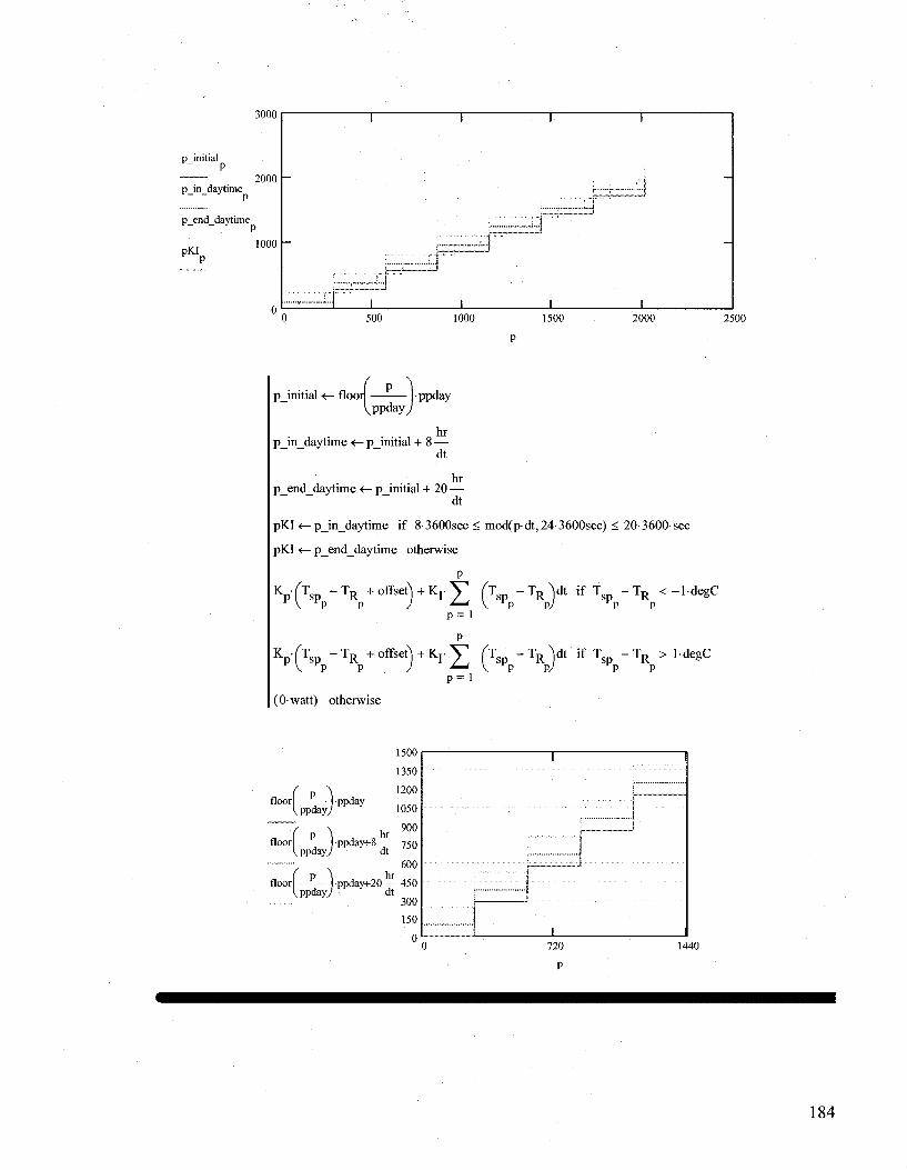
pinitial

p_in_daytime

3000

2000

p_end_daytime

pKI 1000

„ p=3 ,„ L

, .,."„",..,.,. i

. . .rrr** :—*

500 1000 1500 2000 2500

pinitial <— flooij |ppday Vppday,

p indayt ime <— p_initial + 8-hr

dt

hr penddaytime <— pinitial + 20—

dt

pKI <- p_in_daytime if 8-3600sec < mod(pdt,24-3600sec) < 20-3600-sec

pKI <— penddaytime otherwise

P

K p( T s P p - T R p + of fse t) + K r S (TsPp"TR

P)dt if T s P p - T R p <- l d e g c

p = l

S- ( T s P p - T R p + offset) + KrZ

p = l

(Owatt) otherwise

T s P - T R d t i f Tsp " T R > l d e 8 C

floor

floor

floor

PPday,

P ppday

P ppday.

ppday

. hr

1500

1350

1200

1050

900

ppday+8 — 7 5 0 dt

600

ppday+20-F 450

300

150

0

I ' ^

720 1440

INITIAL CONDITIONS:

Node temperatures:

floormass

T floorin.

T wallsmass.

T, wallsin

exmass,

exout

ceihngmass.

ceilingin

T • gin.

gout

lsh.

gap,

*R,

gmid

'sp

21

22

23

24

25

26.5

22.1

22.5

29

10

20.2

20.1

22.7

12

V 1 8 y

•degC

1 J

CONVECTIVE AND RADIATIVE COEFFICIENTS- initial values

Exterior heat transfer coefficient for window surface:

og,

1.81-j T0 l (^out),

1.382

2

w m 2 K

+ 4-E -CT-

Tgout, + T0 )

IA + 273 K

h = 31.325-1 W

n2 degC

Exterior heat transfer coefficient for wall surface:

,„.j T - T o. exout.

1.382 + 1.6

1.81 3 1 T - T o1 exout. \2

V + I2.5-V

1.382 0.75^

o

,,,.J T - T o. exout.

+ 4e w t r .

T + T o exout >* i 3

+ 273 •K

1.382

W

m 2 K

Radiation coefficients:

T g i n i + 273)K 4 r T f + 273 |K gout i ; J

Ewindow

rS, T„;„ - T , glllj gOUtj

rgmidl.

T • +273^K gin 1 )

T g m i d / 2 7 3 ) ^ ewindow

Tginj ^ m i d j

rgmid2

T g o u t l+ 2 7 3 ) K

-\4 r, " ( T g m i d ^ 2 7 3 ) ^ •F. ewindow

^out j V n i d !

"sh.g, •=

Tsh]+273JK T„;„ + 273~\K gin

F e F sh_g

• J 1 T

... between shade and glazing

T s h ] + 273^K

[1sh floor

T f l o o r i n ^ 2 7 3 ) ^ 4 F F e win floor

T — T sh floorin

...between shade and floor

shceiling

T s h ] + 273^K ^eilinginj + 2 7 3 ' K • F -F e winceiling

T — T sh ceilingin

...between shade and ceiling

T s h ] + 273^K T w a l l s i n i+ 2 7 3 ^ K F F e win walls

sh walls T — T sh wallsin

...between shade and walls

gfloor.

T g i n ] + 273)K ~\A

T f l o o r i n i+ 2 7 3 ) K "

F F e win floor

IT . — T gm floorin

...between glazing and floor

186

"g_ceiling1 :"

T g i + 2 7 3 ^ K Tceilinginj + 2 7 3 J K -F -F E win_ceiling

T • — T gin ceilingin

...between glazing and ceiling

g w a l l s '""

T g i n ^ K 1 4 r "Twallsiiij + 2 7 3 j K F F 6 win walls

T -— T gin wallsin

...between glazing and walls

T f l o o r i n ^ ^ K

f loorex •

T e x i n i+ 2 7 3 ) K "

F F e floor south

T — T floorin exin

...between floor and south wall

floor walls

T f l o o r i n ^ 2 7 3 ) * ] ~ [ ^ w a l l s i ^ + 2 7 3 ] K i 4 F • F

e floor walls

T — T floorin wallsin

...between floor and walls

floor_ceiling ' •i ;

Tfloorin, + 2 7 3 ) K 1 " ffTceilingin, + 2 7 3 > ~ F F e floor south

floorin ceilingii

...between floor and ceiling

cei l ingex

Tcei l ingi n i + 2 7 3 ) K

4 r, T e x i n i

+ 2 7 3 ) K • F F E cei l ingsouth

T — T ceilingin exin

...between ceiling and south wall

cei l ingwalls

Tcei l ingi n i + 2 7 3 ) K Twallsin1

+ 2 7 3 >K •14 F F

B cei l ingwalls

T — T ceilingin wallsin

...between ceiling and west wall

ex walls

T e x i n / 2 7 3 ) ^ •i4 r

Twallsinj + 2 7 3 ] K F F E south walls

T — T exin, wallsin,

south wall to walls

Convection coefficients:

watt h c g l a s s . ^ 2 - 5 ^

1 m degC

watt cglass mid l , : = 2 - 5 "

1 m degC cglass_mid2 2.5-

watt

m degC

N u l j := L 1 8 N u l m i d l , := 1.1 Nul mid2, := 1.18

Nu2, := 1.1 Nu2_midl1 := 1.1 Nu2_mid2i := 1.1

watt kwin := 0 . 0 2 3 5 — —

1 m- degC watt

k w i n m i d l := 0 . 0 2 3 5 — - — - 1 m- degC

watt k win mid2, •= 0 . 0 2 3 5 — —

- 1 m-degC

187

Ra[ := 7500 Rajnidl! := 7500 Ra_mid2! := 7500

"win. : = 0A ^ v i n m i d l , ^ 0 1 awin_mid2] : _ °-1

T g mean := 1 0 d e S C

P U„„ := 1.8

W eg l 2

U„ :=2.5-watt

m degC "' m2degC

hcfloor1 :_ 1 - 3 1 ' r T R 1 " T f l o o r i n 1 ^

3 W-degC ... room air to floor

cwalls .31 T — T R. wallsin 3 W-degC ... room air to walls

1.31 TR, Texin, 3 WdegC ... room air to south exterior wall

c 8 , 1.31 T V T s i n i

3 WdegC room air to glass

ncsh. 1.31- TR, ~ Tsh, 3 WdegC room air to shade

gapsh 1.31/ T — T gap, sh, 3 WdegC ... air gap to shade

cceiling 1.31 T — T R. ceilingin

3 WdegC ... room air to ceiling

gapg, ' 1.31 T - T • gap, gin,

3 WdegC

- 4

air gap to glass

FIN

ITE

DIF

FER

EN

CE

MO

DE

L (

SY

ST

EM

OF

EQ

UA

TIO

NS

) M

AT

RIX

:

1.81

? T

- T

o

sout

p

- PI

1.38

2 +

2.

5-V

. 0.75

w

H

T-K

• +

4

-BW

-CT

-

>

Tgo

ut

+

Tsk

y 1-

* 12

.+ 2

73

1,1

.| T

-

T

o ex

out

1.38

2 •+

1.6-

1M1 o

exou

t

1.38

2 +

2.

5-V

. 0.

75

r '•

"•J

T

— T

o

exou

t

1.38

2

W

A

• +

4-

s-a

in-K

[(H

+273

)'K [(

Tg

ou

t/ 2

73V

K

•F, sw

indo

w

T

• —

T

am

sout

, -

P e

p|

[fa+™

)^-[

(^s™

y] •

F sw

indo

w

W,+

27

3* F

giii

j gm

id1

•rT

gim

di

+

273)

Kj

•F, sw

indo

w

Tgo

utj

Tgm

idl

Tsh

+

273

VK

T

pa p

+ 2

73V

K

-F

.p

8 sh

_g

T

— T

I

sh

•'g

in

p Pi

[(Tsh

p +

27

3)'

K]4 -

[(T

floo

rmp +

2

73

)KJ

e w

in f

loor

T

— T

1 s

li 1f!

oonn

Tsh

+

2731

^

'-[(

Tc

eil

mg

in/2

73

) F

F s

win

cei

ling

T

— T

sh

ce

iimsi

n ,

p Pi

00

rTsl

l +

27

3V

K .14

Tw

alls

m

+2

73V

K

• P *

P s

win

wal

ls

Tgi

n +

2

73

^K

T

— T

I

sh

wal

lsin

P

PI

Tfl

oo

rui

+

27

3Y

K

P J

. s

win

fl

oor

T

• +

273

-

P

)*r T

—

T

sin

floo

rin

" P

p

Tce

ilin

gin

+2

73

^ ,P

.p

s

win

cei

lina

a-IT^+2

73)'KJ IT

_

T

gin

ceili

ngin

^

P °

PI

r/Tw

ails

in

+2

73

VK

1 *P

*P

s 'w

in w

alls

T

• —

T

gi

n w

alls

in

Tfl

oori

n +

27

3V

K

Tex

in

+

27

3)K

~ p

J •

P

«P

s fl

oor

sout

h

IT

— T

floo

rin

exin

P

P (T

floo

rin

+2

73

VK

A

P

-14

Tw

alls

iQ

+2

73

VK

| • P

»P

s

floo

r w

alls

IT

— T

I

floo

rin

wal

lsin

P

PI

2

73

VK

.14

'flo

orin

;

T

4- ^

73

^ ~K

ceil

iagi

n ~

r~/-'

i-1^

•F

-F fl

oor

sout

h

'p

T

I fl

oori

n ce

ilin

gin

p P

i

T

-v

• +

273V

K

ceilu

igm

T

i-;J i

^

Tex

ki

+27

3YK

P

/

-s

ceil

ing_

sout

h

IT

— T

I

ceil

ingi

n ex

in

P PI

ceiii

ngin

+

2

73

'VK

'fT

wal

lsm

+

27

3)"

K

A

P J

_ F

F e

ceii

ing_

wal

ls

( ex

in

+ 27

3V K

T

— T

ce

iiin

gin

wal

lsin

Tw

aUs,

n +

27

3V

K

•F *

F s

sout

h w

alls

T"

T

exin

w

alls

in

1.31

./ T

—

T

iR

^llo

orin

, ,

W-d

egC

-4

3

1.31

-f V

R

* w

alls

in

W-d

egC

m

1.31

T

—

T

R

^exi

ii W

-deg

C

in

1.31

-R

ce

iiing

in ,

P

Pi

3 W

-deg

C

1.31

-T

R

~T

2in

, p

~ Pi

3 W

-deg

C

1-31

-/- |

TR

-T

dl

p P

y W

-deg

C

/ 2

1.31

T

—

T

sap

sli

e *p

P

3 W

-deg

C

f I

5 #

SK Lsf*

•I 8.

J*

+

#

192

<£3

<

+ M

v

<

I wH

P

<|<*>

«

o o

'"Si

'5 c4

© ©

+

Q» 4-o

60

.a

J* T «.*• ?

C3

XJ* JF

J

XJ

g i. •? t

•s' -a

193

h ccei

img

, =p

+i

^csh

,

p+i

\gla

ss

, "

p+

i

cgia

ss m

idl

,

"cgl

ass

mid

2 ,

p+1

NB

l_m

idlj

H.j

Nu2

_mid

lp+j

N»2

_Biid

2p+j

"win

,

a wia

mid

l ,

p+i

>0

100-

degC

f gi

n * T

gmid

|

13 +

273

!

100-

degC

/ T

-i-

T

^ go

ut

T

'pa

id

I -

-+ 2

73

V. 2

J J T

gto

+

Tgo

ut

0.00

2528

- +

273

j w

att

T

- -s

-T

ai-d

egC

• 2

73

+ 2

00

0.00

2528

-'T

gia

p +

Tg

mid

p

\l-5

+ 2

73

\ w

aft

T

- +

T

gin

' ni

-deg

C

• +

273

+ 2

00

0.00

2528

-' *g

owt

+

Tgm

id

J-5

+

273 ./

wat

t

soot

"*"

am

id

ni-d

egC

-27

3 +

200

2-*m

Y-(

**m

)4'(

it.

\3

8/

W

K. T

goii

t ?

Tg

inp

'cav

ity

s m

m _

>

"aan

.3

•g

J H I

J

UP

.a sd O

<

S3

S

•S

JP

N*

f

J

Ji

I 3 •9

J

<J3

1.

o

8

l l J

J

+

«?

f

3

hi I

J

j J3

I +

1

j 1 if

J-. _ & 4-

"3 :s a B

195

II

?

I

+

H * 4

i

!

i

5

1.

+

l

^

03

as

IJ

#•

>

"3

t

1

i +

1

<

1

+

J\

+ •a

«?

I

$

U ™ > „-,™™™J

1

.53

+

J3

I =i »*• c

196

II

*"0 u 'S J3

en

'8

J +

|

m P

+

Pf

ftT £8

H 1

1

1

9 u *£3

*o O .a

r™1

i f

•1

if* I

J

if

Wi

J +

1 • 9

^3

i1

•Tfl

1 s$*

.g

+

wf

'S3

ss fti

M

1 £ 4,

*a & 3 oi

fir i f

6 ^

J3

f

J <

M

, '8

197

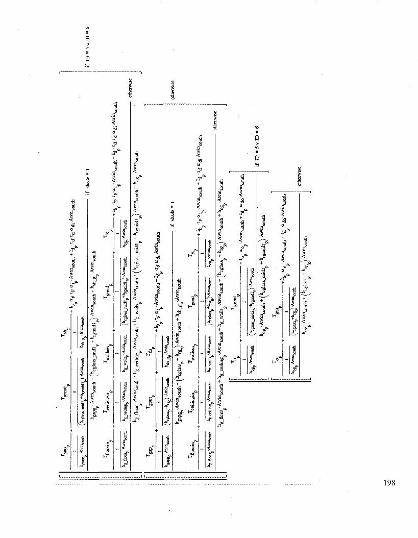
II

> II

a

*3

I

1 f v .'Oi

.<f

if

.3 <

+

j f

1 .3

&P"

+ 1

+

s

+ •3

jp

$

<

f 3

J

•f

•a B

I .a +

+ *0

df1

.2

1

+

i •3

•a +

,1 XI

o

3

.a I

+

II

0 > II Q

,1

(-4 If-

I1

+

1

+

+

0

+

+

198

gout

*g

jn

PP

. P

rfhcg

fass

_mid

l +

hrg

mid

l V

fhcg

lass

m

id2

+ h

rgm

ii2

lTA

wB

,soai

h L

\ P

P

/ V

~~

P

P

/J

floo

rki

ceili

agin

T

wal

ls m

• + I

b 'f

e •

«sh

'Al,

riaso

uih

+Id

-id

e'°-

05-A

wm

; P

P

P

kgs

pshp

'Aw

ife,

A

^J

pA

wi

,W

i ^

Jta

pA

aii

Ba

«&

V

.«a%

"A,™

»<w

&

^w

SE

kp

A^

îA

b<

^-A

wiB

s«fl

i

hsa

psh

-A

wi

lW

i +

hsh

_g •

Aw

raso

«th +

hrf

i fl

oor

'Aw

!« Soi

Mh

* K

h ce

iisng

•A

w«n

So«

th +

hsh

wal

ls -

A™

s©B

th +

h«

h -A

wi

lW

h -"

»*

p

-=

p

- p

P

P

p

P„

xsh

Wp

'Alr

iaK

**

Vp

*p'A

wI£

W*

jafg

apex

t in

fgap

room

hg

ap

8L

'Aw

"Wk +

hga

p& -

Aw

k,*

w!h

*

"""P

p

infg

aspe

xt

iafg

apro

om

dt

Tfiocm

n T

R

Tca

ltng

iii

%

Tw

alls

k TR

Tsh

TR

Tex

tn

TR

To

T

R

Tad

j T

R

Tga

p TR

P

P

P P

P

p

P P

P

P

P P

,

P

P

infe

x î

nfitd

j ^

nfs

+

Qff

lt +

Q;

mt

âu

x

igap

room

dt

ciio

or 'A

fioor

^x

eifa

gp'A

ceJl

iag

Wai

ls '

-V-a

ll ê

stu'

Aw

m«»

tti

\<s£

pAso

u&

Tfl

oort

a ~

%

Tce

tlsag

in

_ T

R

Tw

alki

n _

TR

Tg

ia ~

TR

T&

ri»

_T

R

To ~

%

Tad

j _

TR

Tga

p _T

R

P P

P

P

P P

P

P

P P

,

P

P ,

P

P

P

P +

Qin

t +Q

a

/fk

wc

"css

iliEg

p^ce

fliog

"W

alls

'"w

aif

"s:j„

'Aw

m»n

afa

\nsJ

-Ssa

iA

R

R

R

Mtit

xa«

x 'S

iifex

î

ofiid

j ia

fgap

room

. ?

p

+ T

R

if s

hade

= I

+ T

o ot

herw

ise

\ P

F

./

-..

P

H/

\ V

Y

s \

P

P

X

^„

*-

F

H/

Q-w

att

p =

pK

I p

— p

KI

(0-w

att)

ot

herw

ise

if

s*as

oa *

1

LL K

-(l

-

TR +

ofe

«\

+ K

ry

f'T

~T

RV

* if

fTsp

_

TR

5-2

-deg

C:x s

A(6

-360

0-se

c<m

od(p

.dt,

24-3

600-

sec)

<22

-3»0

-sec

) P

s ¥"

" i

—<

I

pp

p./

V F

p

p

J

\ P

P

p=

pKJ

V(T

* _

TR

-°f

f^)

+ %

Z

(T"p. -

TR

)*

if (

Tsp "

Ts-

- 1

-**c)

p =

pH

(0-w

att)

ot

henv

ise

if

seas

on :

(0-w

att)

ot

herw

ise

3000

2000

UXp

•1000

rffltfiii . 96 98 100 102 104 106 108

dt P'hr

110 112 114 116 118 120

\

sPn

Results:

AIR TEMPERATURES:

200

SURFACE TEMPERATURES

T •

Tshp

T flooriru

T floormass

Tgoutp

wallsin

ceilingin^

Texinp

T °P

35

30

25

20

15

10

5

0

-5

-10

"15

-20

:t&i&$^4m''sm'W&' WS'l

134 136 138 140

PTr

CONVECTIVE HEAT TRANSFER COEFFICIENTS

"cglassp

CgP

shp

"cfloor„

gapgD

gapshp

128 130 132 134 dt

PTr

136

X : X , _ ^ _ ^ £ 1 X ,

138 140

201

RADIATIVE HEAT TRANSFER COEFFICIENTS

\ Sp

n * - g n

nsh floor, P 3

floor wa!ls„

Analysis of energy consumption:

( n d a y s - l d a y ) startt :=

dt startt = 1.728 x 10

168 *" dt

endt := ("days)

dt endt = 2.016 x 10

Energy consumption for full day: 144hr

dt

•dt= 4.309 kW-hr

164 . hr

Energy consumption for occupied hours: I p =

152hr

•dt= 1.932kWhr

Heatingp := iff' Q a u x > Owatt, Q a u x • dt, OkW- hr) Cooling,, := iff Q a i l x < Owatt, Q a , l x • dt, OkW- hr =P • ^aux ^ " " " " ' ^ a u x P P

168-hr

Heating energy consumption for full day: Z lHeati"SP| = 4-309kW.hr 144hr

dt

I -'dt

Cooling energy consumption for full day: "V |coolingp| = OkW-hr

144hr

http://4-309kW.hr

n_p:=

n d a y s - l d a y ( n d a y s - l d a y

dt dt + 1

N ^"days^

dt .timesteps for last day

'n_p —

1

2

3

4

5

6

7

8

9

10

1

12.713

11.754

10.569

9.183

7.626

5.931

4.135

2.273

0.385

0

'sh n_p

kg

1

2

3

4

5

6

7

8

9

10

1

12.267

12.225

12.183

12.14

12.098

12.055

12.012

11.979

11.956

11.94

n_p

n_p

1

2

3

4

5

6

7

8

9

10

1

-21.007

-21.056

-21.103

-21.149

-21.194

-21.238

-21.281

-21.323

-21.364

-21.404

1

2

3

4

5

6

7

8

9

10

1

18.198

18.142

18.088

18.035

17.982

17.93

17.924

17.925

17.929

17.933

gin n_p

1

2

3

4

5

6

7

8

9

10

1

-0.351

-0.394

-0.437

-0.481

-0.525

-0.571

-0.617

-0.663

-0.699

-0.729

n_p

1

2

3

4

5

6

7

8

9

10

1

0

0

0

0

0

201.399

237.116

249.631

258.54

266.471

w

Total fenestration U-value:

Center of Glass:

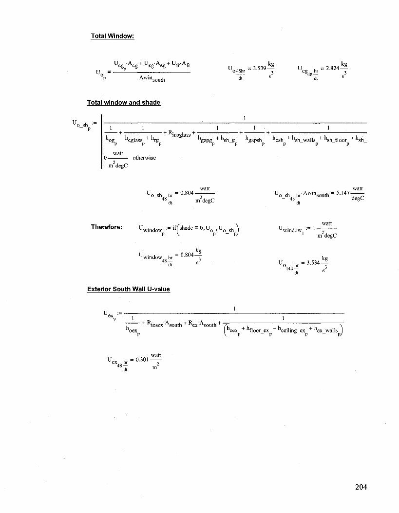
Total Window:

u„

U c g pA c g + U e g A e g + U f r A f r

Awin south

U 0 4 8 ^ = 3 - 5 3 9

dt

kg kg

7 Vs: = 2 - 8 2 4 7 s dt s

Total window and shade

u o sh ' - P

hog hcglass """"rg

watt 0 otherwise

m degC

1 1 — — + R i n sg l a s s +

h + h 'gapg + hsh_g hgapsh hcsh + hsh walls + hsh floor + hsh ° roy> - °p P P ~ P — P ~

watt Uo_shQhr = 0-804 —

48 ^ rndegC

watt U o sh hrA w i nsouth = 5 - 1 4 7 - 7 ~ 7 ; - 48 — degC

dt

Therefore: Uwinf1ftW := iff shade = 0, U0 , U0 s h

P ~ B

watt window, - 9

1 m degC

Uwindow hr = ° - 8 0 4 i 7 4 8 d , u v - = 3 - 5 3 4 7

Exterior South Wall U-value

U ex ' .

P 1 + ^nsex'Asouth + Rex'Asouth +

cex floor ex ceiling ex + ex walls P - P P P,

watt Uex hr = ° - 3 0 1 - T

204

Total U-Value (Glazing, Shade, exerior wall):

facade • , . P (WWR) + (1 - WWR)

IT IT window ex

P P

i watt f a c a d e ^ | = •* 4 - — „ ^ ( W ^ - H J = 4

dt

SUMMARY: _ . , , u „ . = 2.816-^ Center-of-glass: cg\44- 3

dt s

kg Total window: u . = 3.534— ° 1 4 4 ^ ,3

dt s

Total window and shade: uw i n d o w hr = 0.804-^ 4 8 - r o 3

Exterior Wall: u = 0.301 48 —

dt

dt

kg 3

s

s

Total facade: u facade hr = 0.544^ 4 8 d t

APPENDIX D: Indoor thermal environment and thermal comfort model

INDOOR THERMAL ENVIRONMENT & THERMAL COMFORT MODEL

The following methodology is refered to Algorithms for the calculation of the view factors between human body and rectangular surfaces in parallelepiped environments by G. Cannistraro, G. Franzitta, C. Giaconia and G. Rizzo, energy and buildings, 19 (1992) 51-60

Drawings and calculation procedure in this section courtesy of Yu Xiang Chen

Parameters for seated person with known orientation

SEK 1: Vertical rectangle in front of person and above their centre, or behind and below his center SEK 2: Vertical rectangle in front of person and below their centre, or behind and above his center SEK 3: Vertical rectangle on side wall above and forward of their centre, or below and behind his cente SEK 4: Vertical rectangle on side wall below and forward of their centre, or above and behind his cente SEK 5: Horizontal rectangle in ceiling and forward of their centre, or on floor and behind his center SEK 6: Horizontal rectangle in ceiling and behind their centre, or on floor and forward of his center

max '

'0.132N

0.103

0.131

0.104

0.130

v0.101.

A:=

'l.l4505N

1.33522

1.41607

1.15253

1.31858

vl.51966 J

B:=

f0.14524^

0.14454

0.09957

0.13945

0.12807

,0.12266 J

C:=

'0.74379^|

0.60637

0.76196

0.73371

1.00432

^0.84923,

D:=

'0.10312N

0.14678

0.07182

0.09442

0.03802

v0.10471J

F ( a , b , c ) : =

1 - e VB1

max. 1 - e

1 - e A.+B.-

4 4

1 - e 6 6

w-

A3+B3-| -

A5+B5-| -

a

c

K+BJ r

1 - e c i + D f i ! ) + E i ' a

1 - e C2+D2- c + E 2 - ' -

C 3 + D 3 - b + E r

b c

C.+D..-I - |+E.-1 - e

4 4 4

1 - e C 5 + D 5 . - + E 5 . | -

1 - e W!W-

E:=

0.02967

0.04628

0.05578

0.03688

0.06189

^0.05704^

..F() function for 6 SEKs

206

Convert room geometry into dimensionless quantities:

DSC

H P : =

" rnv

:=0.1

:0.6

rm

distance from wall for calculation to start (m)

...seated subject center

D„ H„

\n:=- dis„ DIS

W • win D„ H

V i n ' sp

MR := 12 ...Number of divisons in room in Y direction (rows)

NC := 12 ...Number of divisions in room in X direction (columns)

SF := l.. 8 ...indices of surfaces.

ORT = 1.. 3 ...indices of subject orientation. 1-facing south, 2-north, 3-partition

l iswin:= 0.001

1 south 2 floor 3 west 4 ceiling 5 east 6 north 7 window

NN [ >

V MM Floor Plan

B"

RSpan := • d ^ D S C

M R - 1 ...distance between rows CSpan :=

W r m - 2 D S C

N C - 1 ...distance between columns

mm := 1,2.. MR nn := 1,2.. NC ...indices of locations starting from north-west corner of plan

aa(M,N) :=

w m - [ DSC+ (N - l)CSpan]

w ^ - [ DSC+ (N - l)CSpan]

DSC+(M-1)-RSpan

w ^ - [ DSC + (N - l)CSpan]

D S C + ( M - 1)-RSpan

w m - [ DSC + (N - l)CSpan]

w r m - d i s w i n - t DSC+ (N - l )CSpan] |

D S C + ( N - l)CSpan

D S C + ( N - l ) C S p a n

d j ^ - [ DSC + (M - l)RSpan]

D S C + ( N - l)-CSpan

d r m - [ D S C + ( M - l ) R S p a n ]

D S C + ( N - 1)-CSpan

| [ D S C + ( N - l ) C S p a n ] - d i s w i n |

:= aa(mm,

bb(M,N) :=

h r m _ H p H„

D S C + ( M - l)RSpan dnT1 - [ DSC + (M - l)RSpan]

h rm-Hp H p

D S C + ( M - l)RSpan d ^ - t D S C + C M - l)RSpan]

h r m _ H p

h n n - HP

r m _ w i n - p|

H„

H„

| p ewm|

:= bb(mm,nn)

208

EL

cc(M,N) :=

im-[ DSC + (M - l)RSpan]

H„

[ D S C + ( N - l ) C S p a n ]

h r m _ H p

Wj^,- [ DSC+ (N - l )CSpan]

DSC + ( M - l ) R S p a n

d - [ DSC + (M - l )RSpan]

c m m . n n : = c c ( m m . n n )

1 2

3 4 5 6 7

1 [7.2] [7,2]

[7,2] [7,2] [7,2] [7,2] [7,2]

2 [7.2] [7,2] [7,2] [7,2] [7,2]

[7,2] [7,2]

3

[7.2] [7,2] [7,2] [7,2] [7,2] [7,2] [7,2]

4

[7,2] [7,2]

[7,2] [7,2] [7,2] [7,2] [7,2]

1

2

3

4

5

1

[7,1]

[7.1]

[7,1]

[7.1]

[7.1]

2

[7,1]

[7,1]

[7,1]

[7,1]

[7,1]

3

[7.1]

[7,1]

[7,1]

[7,1]

[7,1]

4

[7.1]

[7,1]

[7,1]

[7,1]

[7,1]

b =

1

2

3

4

5

1

[7,2]

[7.2]

[7.2]

[7.2]

[7,2]

2

[7.2]

[7,2]

[7,2]

[7,2]

[7,2]

3

[7,2]

[7,2]

[7,2]

[7,2]

[7,2]

For subjects facing south Fh, SF

North Wall

North

Ceiling

South Wall

JSEK1

]SEK4

SEK2 r r r - SEK3

SEK5 SEK6

North Wall

FF16(X )Y) :=F[(aX ; Y)6 ) i )(bX j Y)6 j 2 ,(cx ,Y)l1 + F[(aX;Y)6>2!(bXjY)6_2)(cXiY)6]1...

+ F[(aX>Y)6 ) f(bx,Yi6 > i ;(cx,Y)6]2 + F[ (ax ,Y) 6 ^(bx ,Y) 6 r ( cx ,Y) 6 ]2

F16mm,nn := FF16(mm,nn) Fhj 6 := F16

1

2

3

4

5

6

7

1

0.344

0.236

0.188

0.155

0.131

0.112

0.097

2

0.428

0.306

0.233

0.186

0.153

0.128

0.109

3

0.445

0.341

0.261

0.207

0.168

0.14

0.118

4

0.45

0.359

0.279

0.221

0.179

0.148

0.125

5

0.452

0.369

0.289

0.23

0.186

0.154

0.129

South Wall

FFl l (X,Y):=F[(a x > y ) i > i , (b X ) Y ) i > i , ( 9 x > Y ) i ] 1 + F[(a X ( y ) i i 2 , (b x > Y ) i ! i > (^ i Y ) i ] 1 . . .

+ F[(ax>Y)]]I>(bx>Yilj2,(cx,Y)1]2 + F[(aX j Y) i ] 2 , (bX ; Y) i > 2 , (cx ,Y) ]]2

F11mm,nn:=FF11(mm,nn) Fh1?1:=Fll

1

2

3

4

5

6

1

0.06

0.067

0.075

0.085

0.096

0.109

2

0.065

0.073

0.082

0.094

0.107

0.124

3

0.069

0.078

0.088

0.1

0.116

0.134

4

0.072

0.081

0.092

0.105

0.122

0.142

5

0.074

0.083

0.095

0.109

0.126

0.147

East Wall

FF15(X,Y):=F[(aXiY)5i i,(bXiY)5>2,(cx>Y)l3 + F[(aX ; Y)5 ) 2 !(bx ,Y)5 ] !(cx ,Y)5]3. . . + F [ ( a X ; Y) 5 i ] . (bx ,Y) 5 r (cx > Y) 5 ]4 + F[(ax,Y) 5^(bx,Yi 5 ] 2 . ( cX,Y) 5]4

F15mm nn := FF15(mm,nn) Fh| 5:=F15

210

1

2

3

4

5

6

7

1

0.048

0.051

0.053

0.055

0.056

0.056

0.056

2

0.054

0.058

0.06

0.062

0.064

0.064

0.064

3

0.061

0.066

0.069

0.072

0.073

0.074

0.073

4

0.07

0.076

0.08

0.083

0.085

0.086

0.085

5

0.081

0.088

0.093

0.097

0.1

0.101

0.1

West Wall ...same as east wall, just switch sub-script 5 to 3

FF13(X ,Y) :=F[ ( a X i Y ) 3 ! i ) (b X ; Y ) 3 > 2 , ( c x , Y ) l 3 + F [ ( a x , Y ) 3 ) 2 ) ( b X ; Y ) 3 j ] , ( c X ; Y ) 3 J 3 . . .

+ F [ ( a x , Y J 3 1 , ( b X ; Y J 3 i , ( c X i Y ) J 4 + F p a x > Y J 3 2 , ( b X i Y ) 3 > 2 , ( c X ) Y ) 3 ] 4

F13mmjnn:=FF13(mm,nn) F h , 3 : = F 1 3

1

2

3

4

5

6

7

1

0.344

0.43

0.448

0.454

0.455

0.456

0.455

2

0.238

0.303

0.338

0.357

0.367

0.371

0.37

3

0.191

0.231

0.257

0.273

0.283

0.287

0.286

4

0.157

0.183

0.201

0.213

0.221

0.224

0.223

5

0.131

0.148

0.161

0.17

0.176

0.178

0.177

Ceiling

FF14(X,Y) :=F[ (a x > Y ) 4 j , (b x > Y ) 4 > 2 > ( c X i Y ) 4 l 5 + F [ ( a x > Y ) 4 j 2 , ( b x > Y ) 4 > 2 > ( c X i Y ) 4 ] 5 . . .

+ F [ ( a X i Y ) 4 i i , ( b X ) Y J 4 > i , ( c X ; Y ) 4 ] 6 + F p a X ; Y J 4 2 ) ( b X i Y J 4 > ] ! ( c X ) Y ) 4 ] 6

F14m m n n :=FFl4(mm,nn) F h 1 4 : = F 1 4

1

2

3

4

5

6

7

1

0.06

0.064

0.067

0.068

0.069

0.069

0.067

2

0.066

0.07

0.073

0.075

0.075

0.075

0.073

3

0.07

0.075

0.078

0.08

0.08

0.08

0.078

4

0.073

0.078

0.081

0.083

0.084

0.083

0.082

5

0.076

0.08

0.084

0.086

0.086

0.086

0.084

Floor

F F 1 2 ( X ) Y ) : = F [ ( a X i Y ) 2 j i , ( b x > Y ) 2 i i , ( c x , Y ) 2 ] 5 + F [ ( a X i Y ) 2 ) 2 ; ( b x , Y ) 2 i , ( c X j Y ) 2 j 5 . . .

+ F[(ax,Y)2 i l ,(bx ;Y)2 ! 2 ,(cX >Y)2]6 + F [ ( a X ) Y J 2 > 2 , ( b X ( Y J 2 2 , ( c X ] Y ) J 6

F12„ FF12(mm,nn) Fh, 2 :=F12

Fh, 2 =

1 n

3

4

5

6

7

1

0.113 r\ A Atz \1. I t U

0.167

0.182

0.192

0.197

0.2

2

0.138 f\ 4~7C\

0.206

0.225

0.236

0.243

0.246

3

0.155

0.232

0.252

0.266

0.273

0.276

4

0.166

0.248

0.27

0.284

0.292

0.295

5

0.172

0.258

0.281

0.295

0.304

0.307

Window

For left and right

Sal(X, Y) := i f f w ^ - [ DSC+ (Y - l)CSpan] > disw i n , l , - l ] ...to decide substract or

Sa2(X, Y) := i f jbsc + (Y - l)CSpan > diswin> 1,-fj add from other parts of

the window area (S for S b K X . Y ^ i f f V - d ^ - H ^ O . l . - l ) s i g n )

S b 2 ( X , Y ) : = i f ( H p > e w j n , l , - l )

For top and bottom

S l t C X . Y ^ i f j h ^ - d ^ - H p ^ M )

Slb(X,Y):=if(Hp>ew i n ,2,l)

...determine the SEK for

top and bottom parts (S

for SEK, 1 for subject

facing south).

FF17(X,Y):=Sal(X,Y)-Sbl(X,Y).F[(ax,Y)7>],(bx>Y)7>1,(9x,Y)7lsiKX,Y)

+ Sa2(X,Y)Sbl(X,Y)F

+ Sal(X,Y)-Sb2(X,Y>F

+ Sa2(X,Y)-Sb2(X,Y)-F

(ax>Y)7]2>(bx,Y)71.(cx,Y)7

(ax,Y)7 ] . (bx,Y) 7 2 ) (cx>Y) 7

(ax,Y)7 2>(bx,Y)7 2 . (cx,Y)7

Slt(X,Y) •

Slb(X.Y)

Slb(X.Y)

F17n FF17(mm,nn) Fh, 7 :=F17

Fh 1,7:

1

2

3

4

5

6

7

1

0.043

0.048

0.054

0.06

0.068

0.077

0.087

2

0.047

0.052

0.059

0.067

0.076

0.087

0.1

3

0.05

0.056

0.063

0.071

0.082

0.094

0.11

4

0.052

0.058

0.066

0.075

0.086

0.1

0.116

5

0.053

0.06

0.068

0.077

0.089

0.103

0.121

Fh, :=Fh, , - F h 1,7

a

F h , 8 =

1

2

3

4

5

6

7

1

0.017

0.019

0.022

0.025

0.028

0.033

0.039

2

0.018

0.021

0.024

0.027

0.031

0.037

0.044

3

0.019

0.022

0.025

0.029

0.034

0.04

0.048

4

0.02

0.023

0.026

0.03

0.036

0.042

0.051

5

0.021

0.023

0.027

0.031

0.037

0.044

0.053

Sum up view factors to verify the accuracy:

SC:=2. . 8

z sc

Fh i ,sc =

1

2

3

4

5

6

7

8

9

10

11

12

1

0.97

0.993

0.999

0.999

0.999

0.999

1

1.002

1.004

1.004

0.997

0.967

2

0.99

0.988

0.993

0.998

1.002

1.005

1.006

1.007

1.006

1.002

0.995

0.989

3

0.991

0.99

0.985

0.984

0.986

0.987

0.989

0.991

0.993

0.996

0.999

0.993

4

0.988

0.992

0.982

0.976

0.975

0.975

0.977

0.981

0.987

0.994

1.003

0.992

5

0.985

0.992

0.981

0.973

0.969

0.969

0.971

0.976

0.984

0.995

1.004

0.99

6

0.983

0.993

0.98

0.971

0.967

0.966

0.969

0.974

0.983

0.995

1.005

0.989

7

0.983

0.993

0.98

0.971

0.967

0.966

0.969

0.974

0.983

0.995

1.005

0.989

8

0.985

0.992

0.981

0.973

0.969

0.969

0.971

0.976

0.984

0.995

1.004

0.99

9

0.988

0.992

0.982

0.976

0.975

0.975

0.977

0.981

0.987

0.994

1.003

0.992

10

0.991

0.99

0.985

0.984

0.986

0.987

0.989

0.991

0.993

0.996

0.999

0.993

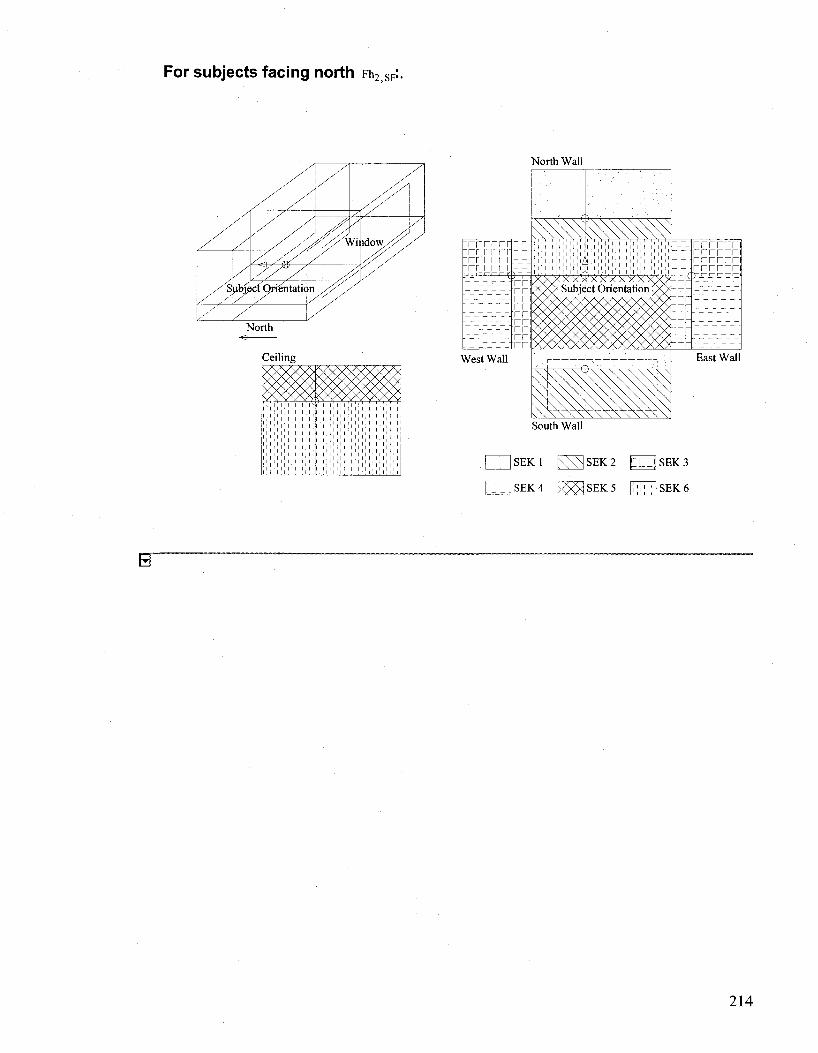
For subjects facing north Fh2 SP-

y

/ / /

/ $ / _,/'

y yhp

y

<itprientatic

X

i \ \ i

n

y

/ X v V i \Aowyy,

kx

North Wall

North

Ceiling

LLLLl

LLLLL

LLLLL

LLLLl

LLLLL

LLLLL

1 1

! 1

- . - „ .-. ~ -

r n r n r n r n r n r n r n r n i i

West Wall

\S 1' 1' 1

N ^ s f ^ ^ s ^ s

l i i ^ i i i i i i i l i i ! xXx x x wx x x x x x >oo< X/V Subject Orientation 5o<

r

iM^

r r T r _ r r _ r r " r r " r r " r r " r r " r r

LLLLL

LLLLL

LLLLL

LLLLL

LLLLL

LLLLL

East Wall

South Wall

SEK 2 [rrrij SEK 3 jSEKl ^ X

] SEK 4 R^xj SEK 5 ^ j ! | SEK 6

214

North Wall

FF26(X,Y):=F[(aXiY)6 ] , (bX ; Y)6 ^ ( ^ ^ ^ ^ [ ( a x ^ J ^ ^ ^ y ) ^ ^ ^ ^ ) ! ! ...

F26mm, nn := FF26(mm, nn) Fh2 6 := F26

1

2

3

4

5

6

7

8

g

10

11

12

1

0.341

0.243

0.201

0.17

0.146

0.126

0.109

0.096

0.085

0.075

0.067

0.06

2

0.425

0.316

0.25

0.204

0.17

0.144

0.124

0.107

0.094

0.082

0.073

0.065

3

0.442

0.352

0.28

0.227

0.188

0.158

0.134

0.116

0.1

0.088

0.078

0.069

4

0.447

0.371

0.299

0.243

0.2

0.168

0.142

0.122

0.105

0.092

0.081

0.072

5

0.45

0.381

0.31

0.253

0.208

0.174

0.147

0.126

0.109

0.095

0.083

0.074

6

0.45

0.385

0.315

0.257

0.212

0.177

0.149

0.128

0.11

0.096

0.084

0.075

7

0.45

0.385

0.315

0.257

0.212

0.177

0.149

0.128

0.11

0.096

0.084

0.075

8

0.45

0.381

0.31

0.253

0.208

0.174

0.147

0.126

0.109

0.095

0.083

0.074

9

0.447

0.371

0.299

0.243

0.2

0.168

0.142

0.122

0.105

0.092

0.081

0.072

10

0.442

0.352

0.28

0.227

0.188

0.158

0.134

0.116

0.1

0.088

0.078

0.069

South Wall

FF21(X,Y):=F[(ax iY)1>1,(bx,Y)1;2,(cx>Y)1]l+F[(ax,Y) i (2,(bx>Y) i2 )(cXiY) i]1...

+ F[(aX ) YJ i > i , (bX YJ i > i , (cX i Y) i] 2 + FpaX i YJ i ^ ( b x ^ j ^ j . ^ Y ^ J

F21mnl;nn := FF21(mm,nn) Fh2>i := F21

1

2

3

4

5

6

7

8

9

10

11

12

1

0.053

0.059

0.066

0.074

0.084

0.097

0.112

0.131

0.155

0.188

0.236

0.344

2

0.057

0.064

0.072

0.082

0.094

0.109

0.128

0.153

0.186

0.233

0.306

0.428

3

0.06

0.067

0.077

0.087

0.101

0.118

0.14

0.168

0.207

0.261

0.341

0.445

4

0.062

0.07

0.08

0.092

0.106

0.125

0.148

0.179

0.221

0.279

0.359

0.45

5

0.064

0.072

0.082

0.094

0.11

0.129

0.154

0.186

0.23

0.289

0.369

0.452

6

0.065

0.073

0.083

0.096

0.111

0.131

0.156

0.189

0.234

0.294

0.373

0.453

7

0.065

0.073

0.083

0.096

0.111

0.131

0.156

0.189

0.234

0.294

0.373

0.453

8

0.064

0.072

0.082

0.094

0.11

0.129

0.154

0.186

0.23

0.289

0.369

0.452

9

0.062

0.07

0.08

0.092

0.106

0.125

0.148

0.179

0.221

0.279

0.359

0.45

10

0.06

0.067

0.077

0.087

0.101

0.118

0.14

0.168

0.207

0.261

0.341

0.445

215

East Wall

FF25(X,Y) : = F [ ( a X ; Y ) 5 i i ; ( b X ; Y ) 5 > ] , ( c X ! Y ) 5 J 3 + F[ (a X i Y ) 5 2 , ( b X ] Y ) 5 2 ) ( c x > Y ) l 3 ...

+ F[(aX,Yi5 ;1>(bx,Yi5)2 ,(cx,Y)5]4 + F[(ax,Y)5 2 .(bx,Yi5 ] 1>(cx,Y)5]4

F25mm, nn := FF25(mm, nn) Fh2 _ 5 := F25

1

2

3

4

5

6

7

8

9

10

11

12

1

0.046

0.049

0.052

0.054

0.055

0.056

0.056

0.056

0.055

0.053

0.051

0.048

2

0.051

0.055

0.059

0.061

0.063

0.064

0.064

0.064

0.062

0.06

0.058

0.054

3

0.058

0.063

0.067

0.07

0.072

0.073

0.074

0.073

0.072

0.069

0.066

0.061

4

0.066

0.072

0.077

0.081

0.084

0.085

0.086

0.085

0.083

0.08

0.076

0.07

5

0.076

0.084

0.09

0.095

0.098

0.1

0.101

0.1

0.097

0.093

0.088

0.081

6

0.088

0.099

0.107

0.113

0.117

0.119

0.12

0.118

0.115

0.11

0.103

0.094

7

0.103

0.117

0.128

0.136

0.141

0.144

0.145

0.143

0.139

0.132

0.123

0.11

8

0.123

0.142

0.156

0.166

0.173

0.177

0.178

0.176

0.17

0.161

0.148

0.131

9

0.147

0.175

0.195

0.209

0.218

0.223

0.224

0.221

0.213

0.201

0.183

0.157

10

0.18

0.222

0.25

0.268

0.28

0.286

0.287

0.283

0.273

0.257

0.231

0.191

West Wall ...same as east wall, just switch sub-script 5 to 3

FF23(X,Y):=F[(^>Y)3 ( 1 , (bx ,Y)3 i l , (cx,Y)3]3 + F[(ax,y)3 i2»(bx,Y)3 )2.(cx,Y)3]3-"

+ F[(ax;Y)3;1»(bx,Y)3>2»(cx,Y)3]4 + F[(aX )Y)3 ;2,(bx,YJ3i l,(cx,Y)3]4

F23m m nn := FF23(mm, nn) Fh.2 3 := F23

1

2

3

4

5

6

7

8

9

10

11

12

1

0.337

0.424

0.443

0.45

0.453

0.455

0.456

0.455

0.454

0.448

0.43

0.344

2

0.228

0.294

0.331

0.352

0.364

0.37

0.371

0.367

0.357

0.338

0.303

0.238

3

0.18

0.222

0.25

0.268

0.28

0.286

0.287

0.283

0.273

0.257

0.231

0.191

4

0.147

0.175

0.195

0.209

0.218

0.223

0.224

0.221

0.213

0.201

0.183

0.157

5

0.123

0.142

0.156

0.166

0.173

0.177

0.178

0.176

0.17

0.161

0.148

0.131

6

0.103

0.117

0.128

0.136

0.141

0.144

0.145

0.143

0.139

0.132

0.123

0.11

7

0.088

0.099

0.107

0.113

0.117

0.119

0.12

0.118

0.115

0.11

0.103

0.094

8

0.076

0.084

0.09

0.095

0.098

0.1

0.101

0.1

0.097

0.093

0.088

0.081

9

0.066

0.072

0.077

0.081

0.084

0.085

0.086

0.085

0.083

0.08

0.076

0.07

10

0.058

0.063

0.067

0.07

0.072

0.073

0.074

0.073

0.072

0.069

0.066

0.061

216

Ceiling

FF24(X,Y) :=F[(aX;Y)4 ^(bx.Y^ ,!>(<*, Y) 4 ] 5 + { k Y ^ . K ^ ^ j U -+ F[(aXiYJ4!i,(bx,Yi4)2,(cX)Y)4]6 + F [ ( a X ) Y J 4 > 2 ! ( b X i Y ) 4 2 , ( c X i Y J 4 ] 6

F24mraj nn := FF24(mm, nn) Fh2 ? 4 := F24

1

2

3

4

5

6

7

8

9

10

11

12

1

0.046

0.052

0.058

0.062

0.065

0.067

0.069

0.069

0.068

0.067

0.064

0.06

2

0.05

0.057

0.063

0.067

0.071

0.073

0.075

0.075

0.075

0.073

0.07

0.066

3 0.053

0.06

0.067

0.072

0.076

0.078

0.08

0.08

0.08

0.078

0.075

0.07

4

0.055

0.063

0.07

0.075

0.079

0.082

0.083

0.084

0.083

0.081

0.078

0.073

5

0.057

0.065

0.072

0.077

0.081

0.084

0.086

0.086

0.086

0.084

0.08

0.076

6

0.057

0.066

0.073

0.078

0.082

0.085

0.087

0.088

0.087

0.085

0.082

0.077

7

0.057

0.066

0.073

0.078

0.082

0.085

0.087

0.088

0.087

0.085

0.082

0.077

8

0.057

0.065

0.072

0.077

0.081

0.084

0.086

0.086

0.086

0.084

0.08

0.076

9

0.055

0.063

0.07

0.075

0.079

0.082

0.083

0.084

0.083

0.081

0.078

0.073

10

0.053

0.06

0.067

0.072

0.076

0.078

0.08

0.08

0.08

0.078

0.075

0.07

Floor

FF22(X,Y) := F[(aXiY)2i,(bx,Y)22,(cx>Y)2]5 + F ^ a ^ ^ b ^ ^ c x ^ ) ! ...

+ F[(aXiYi2]i;(bX;YJ2]i,(cXiY)2]6 + Fpax>YJ2>2!(bXiYJ2i,(cXiY)J6

F22mmj nn := FF22(mm, nn) Fh2 _ 2 := F22

1

2

3

4

5

6

7

8

9

10

11

12

1

0.145

0.169

0.185

0.194

0.199

U.2

0.197

0.192

0.182

0.167

0.145

0.113

2

0.178

0.209

0.228

0.239

0.245

0.246

0.243

0.236

0.225

0.206

0.179

0.138

3

0.199

0.235

0.256

0.268

0.275

0.276

0.273

0.266

0.252

0.232

0.201

0.155

4

0.213

0.251

0.274

0.287

0.294

0.295

0.292

0.284

0.27

0.248

0.215

0.166

5

0.221

0.261

0.285

0.298

0.305

0.307

0.304

0.295

0.281

0.258

0.224

0.172

6

0.225

0.265

0.29

0.304

0.311

0.312

0.309

0.301

0.286

0.263

0.228

0.175

7

0.225

0.265

0.29

0.304

0.311

0.312

0.309

0.301

0.286

0.263

0.228

0.175

8

0.221

0.261

0.285

0.298

0.305

0.307

0.304

0.295

0.281

0.258

0.224

0.172

9

0.213

0.251

0.274

0.287

0.294

0.295

0.292

0.284

0.27

0.248

0.215

0.166

10

0.199

0.235

0.256

0.268

0.275

0.276

0.273

0.266

0.252

0.232

0.201

0.155

Window

Top and bottom

S 2 t ( X , Y ) : = i f ( h n n - d w i n - H p > 0,2,1)

S 2 b ( X , Y ) : = i f ( H p > e w i n , l , 2 )

determine the SEK for

top and bottom parts (S

for SEK, 2 for subject

facing north).

F F 2 7 ( X , Y ) : = S a l ( X , Y ) . S b l ( X , Y ) - F [ ( a X i Y ) 7 ^ , ( b X ) Y ) 7 ^ ( c X i Y n s 2 t ( X i Y )

+ Sa2(X,Y)Sbl(X,Y)F

+ Sal(X,Y)-Sb2(X,Y)F

+ Sa2(X,Y)Sb2(X,Y)F

F27n FF27(mm,nn)

(ax,y)7>2.(bx,Y)7>2.(cx,YJ,

(ax,Y)7 > , ,(bx,Y)7 J ,(qx,Y)7

(a x ,y) 7 2>(bx,Y) 7 , . ( C X , Y ) 7

S2t(X,Y) •

S2b(X,Y)

S2b(X,Y)

Fh •2,7 : F27

Fh2 7 =

1

2

3

4

5

6

7

8

9

10

11

12

1

0.043

0.048

0.054

0.06

0.068

0.077

0.087

0.1

0.114

0.131

0.152

0.202

2

0.047

0.052

0.059

0.067

0.076

0.087

0.1

0.116

0.137

0.162

0.196

0.248

3

0.05

0.056

0.063

0.071

0.082

0.094

0.11

0.129

0.152

0.182

0.218

0.257

4

0.052

0.058

0.066

0.075

0.086

0.1

0.116

0.137

0.163

0.194

0.229

0.259

5

0.053

0.06

0.068

0.077

0.089

0.103

0.121

0.142

0.169

0.2

0.235

0.26

6

0.054

0.061

0.069

0.078

0.09

0.105

0.123

0.145

0.172

0.204

0.237

0.261

7

0.054

0.061

0.069

0.078

0.09

0.105

0.123

0.145

0.172

0.204

0.237

0.261

8

0.053

0.06

0.068

0.077

0.089

0.103

0.121

0.142

0.169

0.2

0.235

0.26

9

0.052

0.058

0.066

0.075

0.086

0.1

0.116

0.137

0.163

0.194

0.229

0.259

10

0.05

0.056

0.063

0.071

0.082

0.094

0.11

0.129

0.152

0.182

0.218

0.257

Fh, :=Fh 2,1 •Fh 2 ,7

Fhi o =

1

2

3

4

5

6

7

8

9

10

11

12

1

i 10 -3

0.011

0.012

0.014

0.017

0.02

0.025

0.031

0.041

0.057

0.084

0.142

2

i-10-3

0.011

0.013

0.015

0.018

0.022

0.028

0.036

0.049

0.071

0.109

0.18

3

0.01

0.012

0.014

0.016

0.019

0.024

0.03

0.04

0.055

0.08

0.123

0.188

4

0.011

0.012

0.014

0.017

0.02

0.025

0.032

0.042

0.058

0.085

0.13

0.191

5

0.011

0.012

0.014

0.017

0.021

0.026

0.033

0.044

0.061

0.089

0.134

0.192

6

0.011

0.013

0.015

0.017

0.021

0.026

0.034

0.045

0.062

0.09

0.136

0.192

7

0.011

0.013

0.015

0.017

0.021

0.026

0.034

0.045

0.062

0.09

0.136

0.192

8

0.011

0.012

0.014

0.017

0.021

0.026

0.033

0.044

0.061

0.089

0.134

0.192

9

0.011

0.012

0.014

0.017

0.02

0.025

0.032

0.042

0.058

0.085

0.13

0.191

10

0.01

0.012

0.014

0.016

0.019

0.024

0.03

0.04

0.055

0.08

0.123

0.188

218


SC := 2.. 8

1

2

3

4

5

6

7

8

9

10

11

12

1

0.967

0.997

1.004

1.004

1.002

1

0.999

0.999

0.999

0.999

0.993

0.97

2

0.989

0.995

1.002

1.006

1.007

1.006

1.005

1.002

0.998

0.993

0.988

0.99

3

0.993

0.999

0.996

0.993

0.991

0.989

0.987

0.986

0.984

0.985

0.99

0.991

4

0.992

1.003

0.994

0.987

0.981

0.977

0.975

0.975

0.976

0.982

0.992

0.988

5

0.99

1.004

0.995

0.984

0.976

0.971

0.969

0.969

0.973

0.981

0.992

0.985

6

0.989

1.005

0.995

0.983

0.974

0.969

0.966

0.967

0.971

0.98

0.993

0.983

7

0.989

1.005

0.995

0.983

0.974

0.969

0.966

0.967

0.971

0.98

0.993

0.983

8

0.99

1.004

0.995

0.984

0.976

0.971

0.969

0.969

0.973

0.981

0.992

0.985

9

0.992

1.003

0.994

0.987

0.981

0.977

0.975

0.975

0.976

0.982

0.992

0.988

10

0.993

0.999

0.996

0.993

0.991

0.989

0.987

0.986

0.984

0.985

0.99

0.991

For subjects facing west /east Fh3 SF:.

[->!>] SEK 4 ggxj SEK 5 []; 5]] SEK 6

I

North Wall

FF36(X,Y) :=F[(a X j Y ) 6 2 , ( b x , Y ) 6 ^ ( c x ^ V F [ ( a X i Y ) 6 ^ K ^ j M ^ -

+ F[(a x > Y ) 6 i 5 (b x > Y ) 6 i ;(cx,Y)6]4 + F [ ( a X j Y J 6 2 ; (b X ! Y J 6 > 2 , ( c X j Y ) 6 J 4

F36mm>nn:=FF36(mm,nn) F h 3 6 : = F 3 6

1

2

3

4

5

6

7

8

9

10

11

12

1

0.336

0.232

0.186

0.155

0.13

0.111

0.096

0.084

0.073

0.065

0.058

0.052

2

0.425

0.304

0.233

0.186

0.153

0.128

0.109

0.093

0.081

0.071

0.063

0.056

3

0.444

0.342

0.263

0.209

0.17

0.141

0.118

0.101

0.087

0.076

0.067

0.059

4

0.45

0.363

0.283

0.225

0.182

0.15

0.126

0.107

0.092

0.08

0.07

0.062

5

0.453

0.374

0.295

0.235

0.19

0.156

0.131

0.111

0.095

0.082

0.072

0.064

6

0.454

0.38

0.301

0.24

0.194

0.16

0.133

0.113

0.097

0.084

0.073

0.065

7

0.455

0.381

0.302

0.241

0.195

0.161

0.134

0.114

0.097

0.084

0.074

0.065

8

0.455

0.377

0.298

0.238

0.192

0.159

0.133

0.112

0.096

0.084

0.073

0.064

9

0.454

0.367

0.288

0.23

0.186

0.154

0.129

0.109

0.094

0.082

0.072

0.063

10

0.449

0.349

0.271

0.216

0.176

0.146

0.123

0.105

0.09

0.079

0.069

0.061

South Wall

F F 3 1 ( X ) Y ) : = F [ ( a x , Y ) i j i , ( b X j Y ) i ) 2 , ( c x > Y ) i l 3 + F [ ( a X j Y ) i j 2 , ( b X ) Y ) i ; i , ( c X ) Y ) i ] 3 . . .

+ F[(ax>Yi1 ;1>(bx )YJ11 ,(cx,Y)1]4 + F [ ( a X j Y J i > 2 , ( b x > Y j ) ^ ( C X . Y ) , ^

F31 m m j n n := FF31 (mm, nn) Fh3 ] := F31

1

2

3

4

5

6

7

8

9

10

11

12

1

0.052

0.058

0.065

0.073

0.084

0.096

0.111

0.13

0.155

0.186

0.232

0.336

2

0.056

0.063

0.071

0.081

0.093

0.109

0.128

0.153

0.186

0.233

0.304

0.425

3

0.059

0.067

0.076

0.087

0.101

0.118

0.141

0.17

0.209

0.263

0.342

0.444

4

0.062

0.07

0.08

0.092

0.107

0.126

0.15

0.182

0.225

0.283

0.363

0.45

5

0.064

0.072

0.082

0.095

0.111

0.131

0.156

0.19

0.235

0.295

0.374

0.453

6

0.065

0.073

0.084

0.097

0.113

0.133

0.16

0.194

0.24

0.301

0.38

0.454

7

0.065

0.074

0.084

0.097

0.114

0.134

0.161

0.195

0.241

0.302

0.381

0.455

8

0.064

0.073

0.084

0.096

0.112

0.133

0.159

0.192

0.238

0.298

0.377

0.455

9

0.063

0.072

0.082

0.094

0.109

0.129

0.154

0.186

0.23

0.288

0.367

0.454

10

0.061

0.069

0.079

0.09

0.105

0.123

0.146

0.176

0.216

0.271

0.349

0.449

2 2 1

East Wall

F F 3 5 ( X ) Y ) : = F [ ( a X ; Y ) 5 i , ( b X i Y ) 5 2 , ( c X j Y ) l 1 + F [ ( a x > Y ) 5 ) 2 , ( b X ! Y ) 5 2 ) ( c X ; Y n i . . .

+ F [ ( a X ) Yi 5 j r (bx,Y) 5 1 >(cx,Y) 5 ]2 + F[(ax>Y)5 ) 2 ;(bx>Y)5 ; l !(cx,Y)5]2

F35m m nn := FF35(mm,nn) Fh3 5 := F35

1

2

3

4

5

6

7

8

9

10

11

12

1

0.047

0.05

0.053

0.054

0.056

0.056

0.056

0.056

0.054

0.053

0.05

0.047

2

0.052

0.056

0.059

0.062

0.063

0.064

0.064

0.063

0.062

0.059

0.056

0.052

3

0.059

0.064

0.068

0.07

0.072

0.073

0.073

0.072

0.07

0.068

0.064

0.059

4

0.067

0.073

0.078

0.081

0.083

0.085

0.085

0.083

0.081

0.078

0.073

0.067

5

0.077

0.084

0.09

0.095

0.097

0.099

0.099

0.097

0.095

0.09

0.084

0.077

6

0.089

0.099

0.106

0.112

0.115

0.117

0.117

0.115

0.112

0.106

0.099

0.089

7

0.104

0.117

0.127

0.134

0.139

0.141

0.141

0.139

0.134

0.127

0.117

0.104

8

0.123

0.141

0.155

0.164

0.17

0.173

0.173

0.17

0.164

0.155

0.141

0.123

9

0.148

0.174

0.193

0.205

0.213

0.217

0.217

0.213

0.205

0.193

0.174

0.148

10

0.181

0.221

0.247

0.264

0.274

0.279

0.279

0.274

0.264

0.247

0.221

0.181

West Wall

F F 3 3 ( X ( Y ) : = F [ ( a x , Y ) 3 1 , ( b x > Y ) 3 ; i , ( c X i Y ) 3 ] 1 + F [ ( a X ; Y ) 3 i 2 , ( b X ! Y ) 3 i ) ( c X i Y ) l 1 . . .

+ F[(ax,Yi3]1.(bx,Yl3>2.(cx,Y)3]2 + F[(ax>Y)3>2.(bx,Y)3 (2.(cx,Y)3]2

F^jn^nu := FF33(mm,nn) FI13 3 := F33

1

2

3

4

5

6

7

8

9

10

11

12

1

0.342

0.424

0.442

0.447

0.45

0.451

0.451

0.45

0.447

0.442

0.424

0.342

2

0.239

0.306

0.342

0.361

0.372

0.376

0.376

0.372

0.361

0.342

0.306

0.239

3

0.195

0.238

0.266

0.284

0.295

0.3

0.3

0.295

0.284

0.266

0.238

0.195

4

0.163

0.192

0.213

0.227

0.236

0.24

0.24

0.236

0.227

0.213

0.192

0.163

5

0.137

0.158

0.174

0.184

0.191

0.195

0.195

0.191

0.184

0.174

0.158

0.137

6

0.117

0.133

0.144

0.152

0.158

0.16

0.16

0.158

0.152

0.144

0.133

0.117

7

0.101

0.113

0.121

0.128

0.132

0.134

0.134

0.132

0.128

0.121

0.113

0.101

8

0.088

0.097

0.104

0.109

0.112

0.114

0.114

0.112

0.109

0.104

0.097

0.088

9

0.077

0.084

0.089

0.093

0.096

0.097

0.097

0.096

0.093

0.089

0.084

0.077

10

0.068

0.073

0.078

0.081

0.083

0.084

0.084

0.083

0.081

0.078

0.073

0.068

222

Ceiling

FF34(X,Y):=F[(aX;Y)4 i2 )(bX;Y)4 i ,(cXjY)4]5 + F[(ax,Y)4>2,(bx,Y)42,(cx ;Y)4]5...

+ F[(ax>YJ4_1,(bx>Yi4)i,(cXjY)4]6 + Fpax > Y)4 > i >(bX YJ4 > 2 )(cx,Y)4]6

F34mm> n n := FF34(mm, nn) Fh3 > 4 := F34

1

2

3

4

5

6

7

8

9

10

11

12

1

0.046

0.051

0.055

0.058

0.06

0.061

0.061

0.06

0.058

0.055

0.051

0.046

2

0.053

0.058

0.062

0.065

0.067

0.068

0.068

0.067

0.065

0.062

0.058

0.053

3

0.058

0.064

0.068

0.071

0.074

0.075

0.075

0.074

0.071

0.068

0.064

0.058

4

0.062

0.068

0.073

0.076

0.078

0.08

0.08

0.078

0.076

0.073

0.068

0.062

5

0.065

0.071

0.076

0.08

0.082

0.083

0.083

0.082

0.08

0.076

0.071

0.065

6

0.066

0.073

0.078

0.082

0.084

0.086

0.086

0.084

0.082

0.078

0.073

0.066

7

0.068

0.074

0.079

0.083

0.086

0.087

0.087

0.086

0.083

0.079

0.074

0.068

8

0.068

0.074

0.079

0.083

0.086

0.087

0.087

0.086

0.083

0.079

0.074

0.068

9

0.067

0.073

0.078

0.082

0.084

0.086

0.086

0.084

0.082

0.078

0.073

0.067

10

0.066

0.072

0.076

0.08

0.082

0.083

0.083

0.082

0.08

0.076

0.072

0.066

Floor

F F 3 2 ( X , Y ) : = F [ ( a x , Y ) 2 i > X ) Y ) 2 i , ( c X ) Y ) 2 V ^

+ F[(ax,Y)2i2.(bx,Y)2tl>(cX,Y)2]6 + F[(aX ; Y)2 > 2 , (bX j Y)2 2 , (cX ; Y)J6

F32mmnn:=FF32(mm,nn) Fh3 2 := F32

1

z 3

4

5

6

7

8

9

10

11

3

1

0.142

0.172

0.192

0.206

0.214

0.218

0.218

0.214

0.206

0.192

0.172

0.142

2

0.166

0.202

0.226

0.242

0.251

0.255

0.255

0.251

0.242

0.226

0.202

0.166

3

0.182

0.223

0.249

0.266

0.276

0.281

0.281

0.276

0.266

0.249

0.223

0.182

4

0.192

0.236

0.264

0.282

0.292

0.297

0.297

0.292

0.282

0.264

0.236

0.192

5

0.198

0.244

0.273

0.291

0.302

0.307

0.307

0.302

0.291

0.273

0.244

0.198

6

0.2

0.247

0.277

0.295

0.306

0.311

0.311

0.306

0.295

0.277

0.247

0.2

7

0.2

0.246

0.276

0.294

0.305

0.31

0.31

0.305

0.294

0.276

0.246

0.2

8

0.195

0.241

0.27

0.288

0.299

0.304

0.304

0.299

0.288

0.27

0.241

0.195

9

0.187

0.23

0.258

0.276

0.286

0.29

0.29

0.286

0.276

0.258

0.23

0.187

10

0.173

0.213

0.239

0.255

0.264

0.268

0.268

0.264

0.255

0.239

0.213

0.173

223

S3_11(X,Y) := ifffh^- d w i n - H p ) [ W r m - [DSC + ( Y - l)CSpan] - diswin] > 0,4,3]

S3_12(X, Y) := ifffh^ - d ^ - H p ) [ W r m - [ DSC + (Y - l)-CSpan ] - diswin] > 0,3,4]

S3_21(X, Y) := if[(hn„- d w i n - Hp)[[ DSC + ( Y - l)CSpan] - diswln] > 0,3,4]

S3_22(X,Y) := i f l h ^ - d w i n - Hp)-[[ DSC + (Y - l)CSpan] - diswin] > 0,4,3]

FF37(X,Y) := Sal(X,Y)-Sbl(X,Y)-Fr(ax>Y)7 1,(bx>Y)7 1,(CX,Y)7]S3_11(XJY)

+ Sa2(X,Y)Sbl(X,Y)F

+ Sa1(X,Y)Sb2(X,Y)F

+ Sa2(X,Y)Sb2(X,Y)F

(ax,Y)7)2,(bx,Y)7;1,(cx,Y)7

(ax;Y)72,(bx,Y)7j2.(cx>Y)7

S3J2(X,Y) -

S3_21(X,Y) -

S3_22(X,Y)

F37n := FF37(mm,nn) Fh3 7 := F37

Fh3>7 =

1

2

3

4

5

6

7

8

9

10

11

12

1

0.034

0.038

0.043

0.048

0.054

0.061

0.069

0.079

0.09

0.104

0.121

0.166

2

0.037

0.042

0.047

0.053

0.06

0.069

0.08

0.094

0.11

0.132

0.163

0.218

3

0.04

0.045

0.051

0.057

0.066

0.076

0.089

0.105

0.125

0.151

0.186

0.228

4

0.042

0.047

0.053

0.061

0.07

0.081

0.095

0.113

0.136

0.164

0.199

0.232

5

0.043

0.049

0.055

0.063

0.073

0.085

0.1

0.119

0.143

0.172

0.206

0.233

6

0.044

0.05

0.057

0.065

0.075

0.087

0.103

0.123

0.147

0.177

0.21

0.233

7

0.044

0.05

0.057

0.065

0.076

0.088

0.104

0.124

0.149

0.179

0.211

0.233

8

0.044

0.05

0.057

0.065

0.075

0.088

0.104

0.123

0.148

0.178

0.21

0.233

9

0.044

0.049

0.056

0.064

0.074

0.086

0.101

0.12

0.144

0.173

0.206

0.232

10

0.042

0.048

0.054

0.062

0.071

0.082

0.097

0.115

0.137

0.165

0.197

0.23

Fh, :=Fh 3,1 •Fh 3,7

Fh-> 0 =

1

2

3

4

5

6

7

8

9

10

11

12

1

0.017

0.019

0.022

0.026

0.03

0.035

0.042

0.051

0.064

0.082

0.11

0.17

2

0.018

0.021

0.024

0.028

0.033

0.039

0.048

0.059

0.076

0.101

0.141

0.207

3

0.019

0.022

0.026

0.03

0.035

0.042

0.052

0.065

0.084

0.112

0.156

0.215

4

0.02

0.023

0.027

0.031

0.037

0.044

0.055

0.069

0.089

0.119

0.164

0.218

5

0.02

0.023

0.027

0.032

0.038

0.046

0.056

0.071

0.092

0.123

0.168

0.22

6

0.021

0.024

0.027

0.032

0.038

0.046

0.057

0.071

0.093

0.124

0.17

0.221

7

0.021

0.024

0.027

0.032

0.038

0.046

0.056

0.071

0.092

0.123

0.169

0.222

8

0.02

0.023

0.027

0.031

0.037

0.045

0.055

0.069

0.09

0.12

0.167

0.223

9

0.02

0.022

0.026

0.03

0.036

0.043

0.053

0.066

0.085

0.115

0.161

0.222

10

0.019

0.021

0.025

0.029

0.034

0.04

0.049

0.061

0.079

0.106

0.151

0.219


SC := 2.. I

^ F h 2 , S C =

SC

1

2

3

4

5

6

7

8

9

10

11

12

1

0.967

0.997

1.004

1.004

1.002

1

0.999

0.999

0.999

0.999

0.993

0.97

2

0.989

0.995

1.002

1.006

1.007

1.006

1.005

1.002

0.998

0.993

0.988

0.99

3

0.993

0.999

0.996

0.993

0.991

0.989

0.987

0.986

0.984

0.985

0.99

0.991

4

0.992

1.003

0.994

0.987

0.981

0.977

0.975

0.975

0.976

0.982

0.992

0.988

5

0.99

1.004

0.995

0.984

0.976

0.971

0.969

0.969

0.973

0.981

0.992

0.985

6

0.989

1.005

0.995

0.983

0.974

0.969

0.966

0.967

0.971

0.98

0.993

0.983

7

0.989

1.005

0.995

0.983

0.974

0.969

0.966

0.967

0.971

0.98

0.993

0.983

8

0.99

1.004

0.995

0.984

0.976

0.971

0.969

0.969

0.973

0.981

0.992

0.985

9

0.992

1.003

0.994

0.987

0.981

0.977

0.975

0.975

0.976

0.982

0.992

0.988

10

0.993

0.999

0.996

0.993

0.991

0.989

0.987

0.986

0.984

0.985

0.99

0.991

Fh:

Fh =

^{12,12} {12,12} {12,12} {12,12} {12,12} {12,12} {12,12} {12,12}A

{12,12} {12,12} {12,12} {12,12} {12,12} {12,12} {12,12} {12,12}

v{12,12} {12,12} {12,12} {12,12} {12,12} {12,12} {12,12} {12,12}J

^{12,12} {12,12} {12,12} {12,12} {12,12} {12,12} {12,12} {12,12}^

{12,12} {12,12} {12,12} {12,12} {12,12} {12,12} {12,12} {12,12}

^{12,12} {12,12} {12,12} {12,12} {12,12} {12,12} {12,12} {12,12}

Z^'^y 1.001

sc ...sum of view factors for given orientation at a given position (x,y)

Correction Factor for View Factors

The algorithm to calculate view factors between a person and surrounding surfaces does not generate results for the sum of view factors that add up to exactly 1.00.. For example, some values add up to 0.975 which is considered accurate for most purposes. However, when calculating the MRT, absolute temperature is used - this means it is a weighted average of view factors and temperatures to the fourth power. These small differences in view factor summation will therefore be amplified when calculating MRT. Therefore, a correction factor is needed in order to force the view factors to add up to exactly 1.00:

X:= 1,2.. MR Y:= 1.2..NC index := 1,2.. 3

CORR(index,X,Y) :=

/ j (Fnindex,Sc) X,Y

SC = 2

ADJ( index, SC,x,Y) := CORR(index,x,Y)(Fhindex sc) ..adjustment of view factors to add to 1.00 A, Y

V ADJ(3,SC,X,Y)

SC = 2

1

2

3

4

5

6

I

Definition of Orientation and Surface Temperatures

ORT := 3 ...indices of subject orientation. 1-facing south, 2-north, 3-partition.

T •=

T, exin

floorin

T, wallsin

ceilinsin P

T wallsin

T, wallsin

T L if shade = 1

T • otherwise P

1 = south (window + wall) 2 = floor 3 = west 4 = ceiling 5 = east 6 = north 7 = window 8 = south wall (spandrel)

4p MRT(X,Y,p) := I V |(ADJ(ORT,i,X, Y))-["(Tp +273)1 4 ] - 273

J i=2

MRT 2 ,8 ,62— = 24.187 dti

Mean projected Area Factor for seated people (fp)

The mean projected area factor (fp) takes into account the position and orientation of the person relative to the sun's position (azimuth and altitude). A new parameter, the "person-solar azimuth angle" is used to define the azimuth angle between the sun and the front of the person (analogous to the surface-solar azimuth angle for tilted surfaces).

Person-solar azimuth angle:

Person's orientation: e per'

(Odeg) if ORT = 1

(180deg) if ORT = 2

(90deg) if ORT = 3

(facing facade = 0, with facade to left, v|/ = +90deg)

Yper • ^s + per ...person-solar azimuth

f ( n , t ) = y Af; ,-(a (n,t))y ' -..a function of solar altitude, a, and person-solar azimuth

angle, yper i = 0

Afr(n,t) = y Kcoeff .as(n,t)j

j = o

K coeff •

2.884-10-1 2.225-10"3 -5.47-10~5 1.802-10"7 '

2.225-10"3 -7.653-10"5 7.286-10"7 -1.457-10"9

-9.292-10"5 4.021-10"6 -6.215-10"8 3.152-10"10

9.027-10"7 -4.632-10"8 7.69-10"10 -4.015-10"12

^-10 12 V-2.51710 1.38-10 -2.341-10 1.231-10

-14

...coeff. of the polynomial algorithm

i:= 1.2..5

A f P , i : = Z j = l

K coeff. .' I.J

180

PV n

( j- l)

per • P

z A f p , i -

i = 1

0 otherwise

per 180

p V n

(i-i) if 12hr- t (n) < mod(p-dt,24-3600sec) < 12hr+t (n)

227

« per

0.4

0.3

0.2

0.1

Projected area factor (occupied hours) 1 I 1 1 1 1 1 1

1 1 L__ 1 1 I I 1

1 i 1

-

-

1 1 1

120 122 124 126 128 130 132 134

dt P h r

136 138 140 142 144

CALCULATION OF MEAN RADIANT TEMPERATURE

MRT due to interior surface temperatures only:

MRT(X,Y,p) := V r(ADJ(ORT,i,X, Y))-["(Tp + 273) 141 - 273

i = 2

MRT due to solar radiation and interior surface temperatures

E := 0.9 ...emissivity of person

a b r := o.8 ...beam absorptance of person a d := 0.5 ••• diffuse absorptance of person

Tfacade Te Tsh ' s a d e ~ ...solar transmittance of facade system with

Te otherwise P

and without shading device

MRTsolar<X 'Y>P> :=

O

V r(ADJ(ORT,i ,X,Y)) |"(Tp+273)l41 ...

i =2

2„4 in K

ad_perADJ(ORT,7 IX,Y)--

1 shade = l ,T s h , lj I j • xjgiflshade = 1

watt

~~2

+ a b_per' per

I b - T e i f ( s h a d e = l , T s h , l ) P P

watt ~~2

273

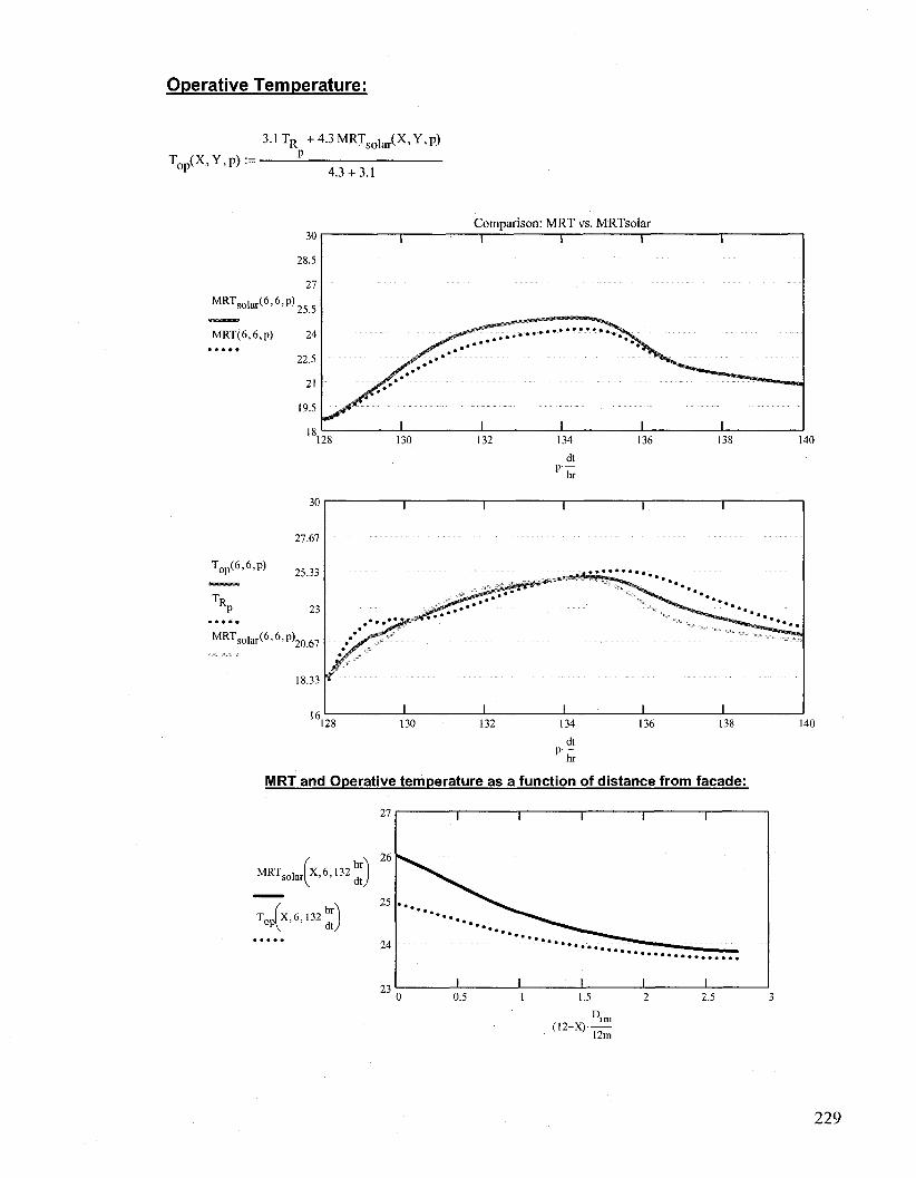
Operative Temperature:

T o p (X,Y,p) :=

3.1 TR +4.3MRT s o l a i{X,Y,p) P

4.3 + 3.1

MRTsolar(6,6,p)

MRT(6,6,p)

30

28.5

27

25.5

24

22.5

21

19.5

i: 128 130

Comparison: MRT vs. MRTsolar

132 134

dt

136 138 140

T o p ( 6 ' 6 ' p )

* * • A •

MRTsolar(6.6>P).

MRT and Operative temperature as a function of distance from facade:

M R T s o l a r [ X A 1 3 2 J

r o p ( x , 6 , 1 3 2 |

(12-X)-12m

229

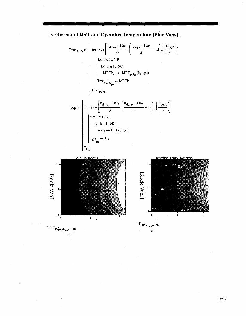
Isotherms of MRT and Operative temperature (Plan View):

Tmrt, solar' for pee n d a y s - l d a y r n d a y s - l d a y

dt •+ 12 ..

'"days'1

dt

for Is 1.. MR

for ke 1..NC

MRTPk?1«-MRT so l a r(k,l,pc)

V dt /

Tmrtso,ar ^ M R T P pc

Tmrt. solar

'OP for pc e ndays-'day fndayS- Iday

+ 12 dt V dt

for le 1.. MR

for ke 1..NC

T0 P k , < - T (k,l,pc)

T o p <-Top

'OP

pc

"days

dt

Tmrt, solarndays-12hr

dt

^ " d a y s - 1 2 1 * dt

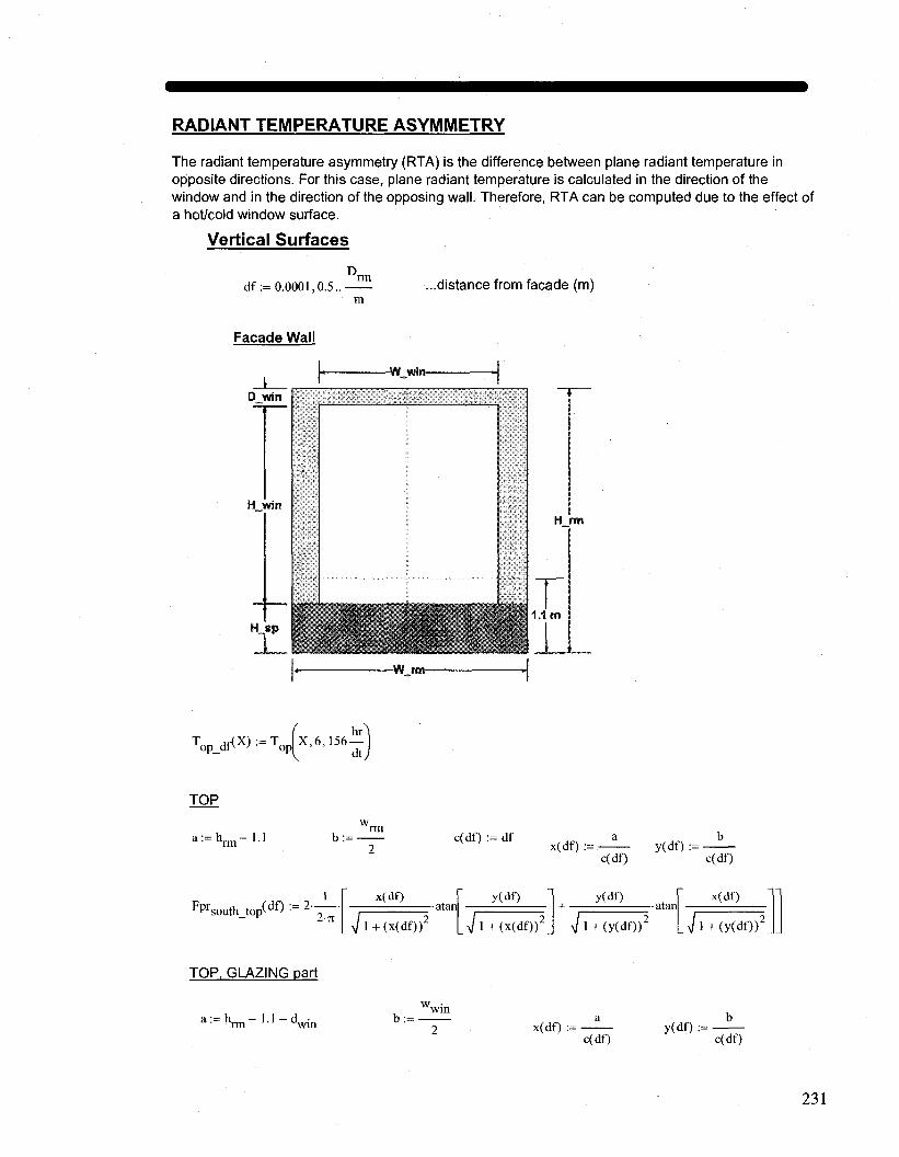
RADIANT TEMPERATURE ASYMMETRY

The radiant temperature asymmetry (RTA) is the difference between plane radiant temperature in opposite directions. For this case, plane radiant temperature is calculated in the direction of the window and in the direction of the opposing wall. Therefore, RTA can be computed due to the effect of a hot/cold window surface.

Vertical Surfaces

D_ df := 0.0001,0.5. ...distance from facade (m)

Facade Wall

i_ D win

H win

H_sp

JL

-W wln-

-W nm-

H rm

1.1 m

T o p _ d f ( X ) : = T o p X > 6 > 1 5 6 -

TOP

a : = h r m - U

FPrsouth_top(df) : = 2"

b:=

2-71

x(df)

c(df) := df a b K ; x(df) := y(df) := •

7 1 + (xi • atari

wr

y(df)

i + (x(df>r

c(df)

y(df)

/

•ataru

1 +(y(df))

c(df)

x(df)

1 +(y(df))^

TOP, GLAZING part

a : = h r m - U - d w i n b:=-x(df) :=

c(df) y(df)

c(df)

231

Fpr, glazingtop^" ) ' 2 ' ~ x(df)

•atartf

I + (x(df))z

y(df)

x/ 1 + (xi (df))

y(df)

7TT •atanl

(y(df))z

x(df)

^ (y(df))'

TOP, WALL part

FPrsouthwall_top(df) : = FPrsouth_top(df) ~ FPrglazing_top(df)

BOTTOM (entire)

a:= 1.1 b:=-x(df) :=

c(df) y(df) :=

c(df)

FPrsouth bottom(df) : = 2 ~ - 2-71

x(df) •ataru

h+(* (df» z

y(df)

/ 1 + (x(df))z

y(df)

7TT •atanl

(y(df))z

x(df)

1 + (y(df))z

BOTTOM. GLAZING part

a:= 1.1-e„ b:= x(df) :=

c(df) y(df) :=

c(df)

FPrglazing_bottom(df) '- 2 ' 2-7T

x(df)

/

• atari 1 + (x(df))z

y(df)

71+(xi (df» z

y(df) t , H atari

yrr (y(df))z

x(df)

7TT (y(df))z

BOTTOM, GLAZING + WALL (edges beside window)

b:= rm y(df) := c(df)

FPrglazing wall(df) : = 2 ' 2-71

x(df)

\/ 1 + (x

•ataru

(df)) '

y(df)

\ / l + ( x (df)) '

y(df) •ataru

/ . + (y(df))'

x(df)

x/l + (y(df))2J_

BOTTOM, WALL

FPrsouthwall_bottom(df) : = FPrglazing_wall(df) " FPrglazing_bottom(df)

BOTTOM,SPANDREL

FPrspandrel(df> := FPrsouth_bottom(df) ~ FPrglazing_wall(df)

TOTAL GLAZING

FPrglazing(df> : = FPrglazing_top(df) + FPrglazing_bottom(df)

TOTAL SOUTH WALL (facade excluding glazing)

FPrsouth_wall(df) := FPrsouthwall_top(df) + FPrsouthwall_bottom(df) + FPrspandreKdf)

Back Wall

TOP

a : = h r m - l . l b :=- c(df):=d - d f x(df) :=

FPrnorth_top(df) := 2 x(df)

"* LN/l + (x(df))2

• atari y(df)

>/ 1 + (x. (df))z

c(df)

y(df)

y(df) := • c(df)

•atari

yj 1 + (y(df))2 [ >/1 + (y(df»

x(df)

BOTTOM

a:= 1.1 x(df) := • c(df)

FPrnorth bottom(df) : = 2 ' 2-7t

x(df) -atari

>/ 1 + (x(df))2 [ N/ 1 + (xi

y(dO

s(df)r

y(df)

;

•atari 1 + (y(df))z

x(df)

/ 1 + (y(df))"

TOTAL NORTH WALL

Fprnorth(df) := Fprn o r t h_ t o p(df) + Fprn<j r th_bo t tom(df)

Side Walls

TOP, FORWARD

a(df):=df b := h — 1.1

x(df) := a(df)

y:=

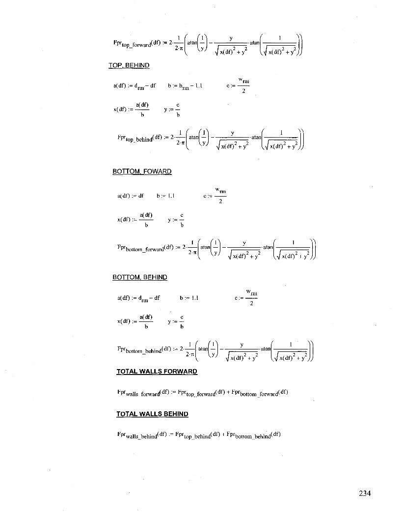
FPrtop f o r w a r d ^ : = 2 " 2- it

[ i 1 y atan — —atan

yJ Jx(df)2 + y2 U*(df)2 +

Y\

• y 2 ; ;

TOP, BEHIND

a ( d f ) : = d r m - d f

, , „ a(df) x(df) := — • —

b

b : = h m i -

c

1.1

FPrtop b e h i n d ^ : = 2 — 2-71

atani / 'A

vy; •atan

>/x(df)2 + y2 Ux(df)2 +

W

y2yy

BOTTOM. FOWARD

a(df):=df b : = l . l

, , n <df) x(df) := y := -

b b

FPrbottom forward(df) : = 2 ' 2-7t ^ ^ ( d f ^ + y2 W x ( d f ) 2

•atan Y*

' + y2;y

BOTTOM. BEHIND

a(df):=d - d f b : = l . l

x(df) := y := -b b

FPrbottom b e h i n d ^ : = 2 ~ — Z-7t

( ( atan I

V

V .yj >/x(df)2 + y2

•atan W

,7x(df)2 vv ^ u i ; + y JJ

TOTAL WALLS FORWARD

FPrwalls_forward(df) : = FP rtopJbrward(df) + FPrbottom_forward(df)

TOTAL WALLS BEHIND

FPrwalls_behind(df> := FPrtop_behind(df) + FPrbottomJ>ehind(df)

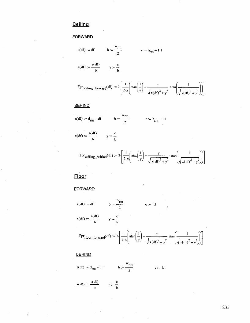
Ceiling

FORWARD

a(df) := df b := : : = h n n - l . l

x(df) := y := -b b

FPrceiling_forward(df) : = 2 ' 2-it

atan vy.

•atan ^x(df)2 + y2 Ux(df)2 +

AY

•y2JJ_

BEHIND

a ^ - d ^ - d f c - h ^ - 1 . 1

M O a ( d f ) c

x(df) := y := -b b

FPrceiling_behind(df) : = 2 ' 2-71

atan Vy \/xi

• atan 2 2

(df) +y 2

Y\l

.>/ x(df)2 + y2))_

Floor

FORWARD

a(df) := df

x(df) := b

b ;

y :

FPrfloor_forward(df)

w rm

2

c

b

= 2-1

2-71 atan

V

c:= 1.1

Vy ^

•atan 2 2

(df) +y 2

>V

.>/x(df)2 + y2JJ_

BEHIND

a ( d f ) : = d r m - d f b:=- c:= 1.1

^ n ^ d f ) c

x(df) := y := -b b

FPrfloor behind(df) : = 2

2-7T atani

y ( i ^ •atan

JJ yjx(d{)2 + y2 Ux(df)2 + y2

;y.

Check for unity:

/'A

FPrglazing(df) + FPrsoUth_wall(df) + FPrwalls_forward(df) + FPrceiling f o r w a r d ^ + FPrfloor f o r w a r d ^ =

W

236

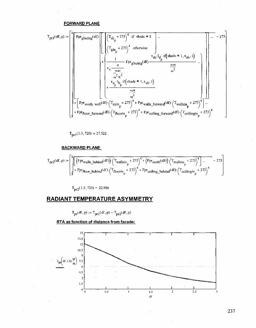
FORWARD PLANE

T p r ](df ,p) := Fpr glazing' (df) Tcll + 273V if shade = 1 sh ;

T • +273V otherwise P

•Fpr glazing' (df)-

T d e I d i f ( S h a d e = 1 ' T s h ' 1 )

m -is.

watt 2

T e - I b i f ( s h a d e = l , T s h , l ) P P v _

watt 2

FPrsouth wall(df)fTexin_ + 2 7 3 V + FPrwalls_forward(df)fTwallsin_ + 2 7 3 1 V J - V P /

+ FPrfloor_foraard(df)-fTfloorin + 2 7 3 ) + FPrceiling_foward(d^fTceilingin + 2 7 3 )

•273

T . (1.5,720) = 27.522

BACKWARD PLANE

V2(df'P):= (FPrwalls_behind(df))(Twallsinp + 2 7 3 ) + (FP rnorth(df))(Twallsinp

+ 2 7 3 ) ,

+ FPrfloor_behind(df>rTfloorinp + 2 7 3 ) + FPrceiling_behind(df)-rTceilingin + 2 7 3 )

•273

T 2 ( 1.5,725) = 22.986

RADIANT TEMPERATURE ASYMMETRY

Tpr(df, p) := Tp H(df,p) - Tpr2(df,p)

RTA as function of distance from facade:

Mdf'132!it

237

RTA as function of time (center of room):

Tpr(1.5m,p) 3

dt P'hr

n_p:=

n d a y s - 2 d a y f n d a y s - 2 d a y

dt dt + 1

n d a y s - l d a y

dt

MRT(6,6,n_p)

P^ rm

V 2m J

1

2

3

4

5

6

7

8

9

10

1

19.427

19.398

19.368

19.338

19.308

19.279

19.25

19.221

19.199

19.182

1

2

3

4

5

6

7

8

9

10

1

-2.93

-2.93

-2.931

-2.932

-2.933

-2.934

-2.936

-2.937

-2.937

-2.935

MRT s o l a r (6 ,6 , tu , )

1

2

3

4

5

6

7

8

9

10

1

19.428

19.398

19.369

19.339

19.31

19.28

19.251

19.222

19.2

19.183

Tpr(df,720)

^11.978^

9.611

6.806

4.793

3.393

2.428

V 1.774 j

T o p ( 6 , 6 , n j )

1

2

3

4

5

6

7

8

9

10

1

18.922

18.882

18.842

18.803

18.763

18.725

18.686

18.67

18.66

18.654

238

THERMAL COMFORT MODEL

This file is used for analysis of thermal comfort based on the principles of human thermoregulation using a transient two-node model. The environmental variables calculated in the building thermal sumulation model (room air temperature, mean radiant temperature) are used as inputs into this model. For this model, several assumptions need to be made for several parameters, such as: clothing insulation, body mass, surface area, metabolic rate, etc. Details regarding the thermoregulation model can be found in the literature (ASJHRAE Handbook, 2005; Parsons, Human Thermal Environments, 2003)

kPa= lOOOPa K = 1

X : = 6 Y := 6 ...position in room (X = distance from window, Y = distance from wall)

f M := 1.2- 58.15-

watt1

...metabolic rate wk := 0 watt ...external work

A D := l.8m ...DuBois surface area mb := 80kg ...body mass RH := 0.5 ...relative humidity

v - :=o.l ...air velocity (m/s) clo := 0.5 if season = 1

0.9 if season = 2 ...clothing insulation

C p B :=3490

C p b :=4187

kgdegC

J

kgdegC

...specific heat of the body

...specific heat of blood

k„„, := 5.28-watt ..thermal conductance between core and skin

T : c r n

Tsk_n

T B n :

m degC

= 36.8degC

:= 33.7degC

= 36.49degC

...neutral core temp.

...neutral skin temp.

...neutral body temp.

Aj :=-5.8002206-10

A 4 := 41.764768-10

A 2 := 1.3914993

A5:=-14.452093-10

-48.640239-10

A 7 := 6.5459673

.-3

...coefficients used for calculating partial pressure at skin

V c L a i r ^ ^ a i r ^ - 2 ' 3 - 1 ' 8 - 3 ' ^ 0.6\ watt

m degC

...convective heat transfer coeffient between clothing and room air

f , := 1 + 0.3-clo ...fractional increase in body surface attributed to clothing

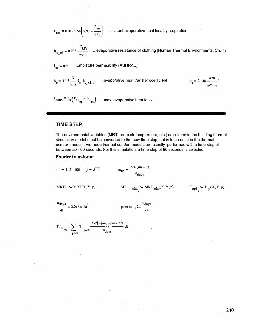
E r e s = 0.0173-M-P .

air 5.87 k?aj

\ ...latent evaporative heat loss by respiration

m kPa R i := 0.033 ...evaporative resistance of clothing (Human Thermal Environments, Ch. 7)

watt

i ^ := 0.4 ...moisture permeability (ASHRAE)

he := 16.5 i j ^ c l a i r ...evaporative heat transfer coefficient he = 20.46-wa

l n in c ci an e -> k P a - " m2kPa

max ~ e'f sk p w p J ...max. evaporative heat loss

TIME STEP:

The environmental variables (MRT, room air temperature, etc.) calculated in the building thermal simulation model must be converted to the new time step that is to be used in the thermal comfort model. Two-node thermal comfort models are usually performed with a time step of between 20 - 60 seconds. For this simulation, a time step of 60 seconds is selected.

Fourier transform:

1,2.. 100 j : = ^ 2 i t ( n n - 1)

<0nn : =

"days

MRTlp :=MRT(X,Y,p) M R T 1 solar : = M R 1 W X ' Y ' P ) Topl : = T o D ( X - Y 'P> P v P F

"days 3 "days — = 2.016x10 paux:=l ,2 . . —

dt dt

ex^-j-o^-paux-dt) TT R :=> T R dt

nn L-t paux nd paux 3

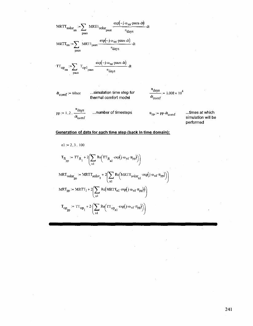
MRTT solar -I MRT1 solar exr^-jonnpauxdt)

paux n paux

days

M R T T n n : = £ MRTlpaux

paux

exp(-j-ff)nnpauxdt)

"days •dt

exp(-j-g)nnpauxdt) T T op : = X Topl d t

i-nn S-l paux nd

paux J

dt

dt m f := 60sec ...simulation time step for thermal comfort model

ndays

dt,

ndays 4 •= 1.008 x 10

dt. Lcomf

PP := 1,2.. '— ...number of timesteps ttpp := ppdtc 0 m f

comf

Generation of data for each time step (back in time domain):

nl :=2 ,3 . . 100

TR := T TR + 2 ( 2 ] M^R -exp(j-o>nr"pp)

M R Tsolar := M R T Tsolar , + 2 | Y R < M R T T s o l a r •exp(j«»nlttpp)

MRTpp := MRTTJ + 2 | V Re(MRTTn lexp(jcon lttpp))

T°PPP 1= TT°Pi + 2 f 2 Re('rropnl-

exP(j-cl)nrttpp)'

...times at which simulation will be performed

241

Initial Conditions:

'sk. 'sk n ..initial skin temperature = neutral skin temperature

..initial core temperature = neutral core temperature

WSIG_ CTi

CSIGcr]

W S I G s k ,

C S I G s k l

WSIGB

SKBFj

\_cl_air

a mass ,

'abs,

sk.

0

0

0

0

0

kg

3.7-

secm

watt

m degC

0.1

36degC

watt 0-

m

313K

5kPa

0

' i ;

f w, ^

^skj

CSj

Qcrsk

res

RS,

cr,

5sk,

Qbi,

Psat,

c w

max

cres, V 1 j

0-

0 >

watt

m

30degC

watt 0-

0 -

m

watt

2 m

watt

2 m

watt

2 m

watt

2 m

watt

2 ni

40 , 2 hrm

2kPa

lkPa

watt 100

20-

m

watt

m

242

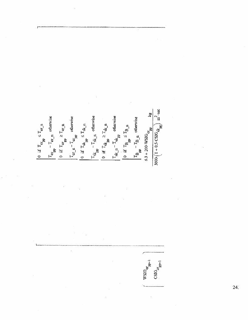
WSI

G cr

pp+

1

CS

Ki cr

PJM

-1

0 if

T

<

T

c,p

p c

r-n

Tc

r -

Tc

r n

othe

rwis

e m

0

if

T

> T

PP

Tc

rti

-T

er

ot»w

wis

e PP

0

if

T*

<T

sk

a PP

""s

k _

^s

k n

°*he

rwis

e '

PP

0 i

f T

sk

&T

sk

Q

PP

Tsf

c o

-'T

sk

°**

™«

e

0 if

T

B

< T

B

n

PP

TR

_T

g n

othe

rwis

e PP

6.3

+ 2

00-W

SIG

cr PP

k

g

36

00

.ri +

0.5

.CS

IGsk

)

m2

PR/

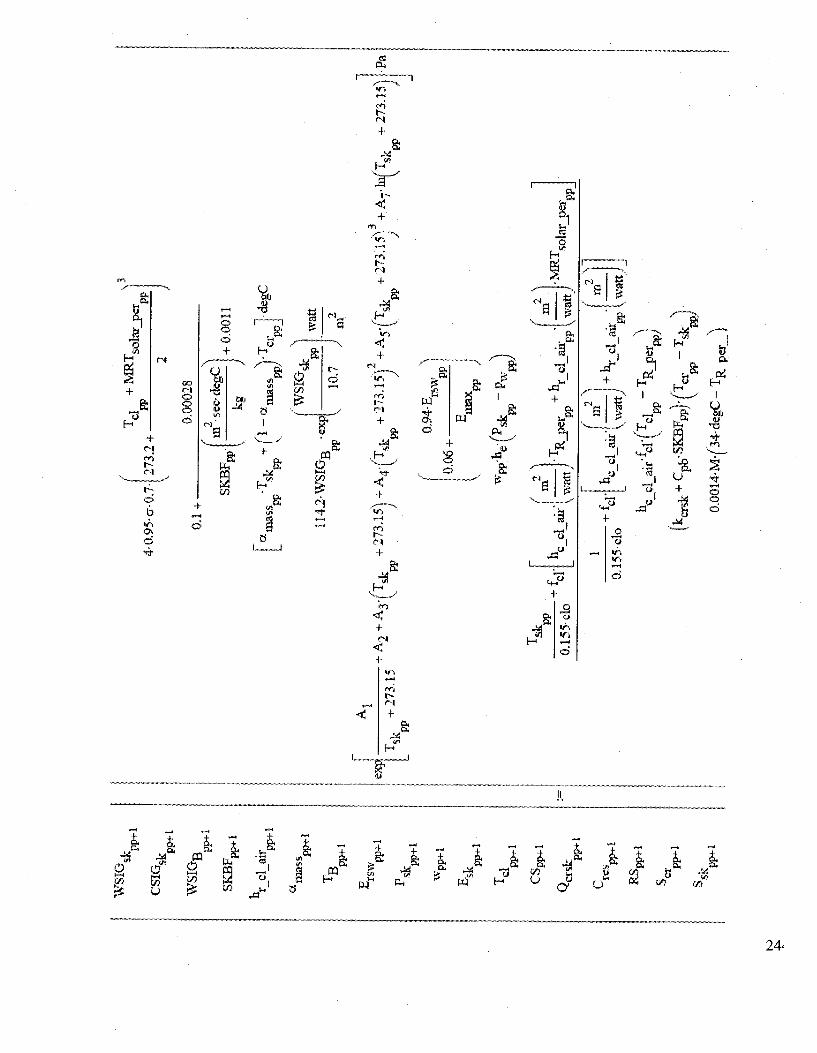
4- 0

,95-

GF-

0.7

-27

3.2

+ •

T

in

—*

<

pp

pp

V

0,1

0.00

028

„„

„„

I nT

-sec

-dee

C I

SK

BFp

p-

—

1 +

0.0

011

kg

114.

2-W

SIG

B

-exd

PP

f'W

SIG

^ )

pp

wat

t

10.7

m

™l\-

-

^T

^A

2+

A3

-(

Ts

k +

27

3.1

5U

A4Y

Ts

k +

27

3.1

5V

+ A

5.(

Tsk

+ 2

73.1

5V+

. A

rk

fT,

Ask

~

ri7

i-15

V

PP

/ V

PP

J

V

PP

J \

' L

P

P

0.06

+

PP

max

PP

J w

pp

-ivrp

sk

-P

w

V

PP

PP,

Tsk

PP

0.15

5- d

o •

+ € •c

l'

2\

k c c

l ai

r"

m

wa

tt J

•T

+ h

R

jper

r

cl

air

-^

PP

- -

PP (

2^

m

•MR

T so

lar_

per PP

1

0.15

5-do

+ 1 •c

l' h c

cl a

ir' (

2 \

m

v wa

tt /

+

hr

cl

air

PP f

2"

m

•y w

att

j

\ el

air

'^cl

'Pcf

TR

_per

\

PP

-^

PP,

(kcr

ek +

CP

b'S

KB

FP

p)f

Ta

' -T

sk

r '

V

PP

PP,

0.0Q

14-M

- (/34

-deg

€- T

R

pe

r

sk

+

PP

R-P

eW

i M

RT

, sola

r_pe

r PP

+1

"pp

+1

lsk fj

p+

i

opjp

er Pf

H-1

Qbi

pp-r

t

Psa

t pp+

1

Pw p

p*

i

'pp

+1

pp

~i

y

expj

PP»'

hr

cl a

ir

,fci

fTcl

_

MR

Ts

ot»

pe

r -

- PP

V

PP

"

^l

'/ P

. PP/

M-W

k-f

Cr

es

+E

re

s

V

PP

v

Qcr

sk

-fC

SP

P +

RS

EP +

E

sk

PP

V

PP..

TR

if 8

-360

0-se

c <

iii

odfp

p-dt

conl

f,24

-360

0-se

c)

< 2

0-36

00-s

ec

PP

if(s

easo

n s

1,24

,0- d

egC

,21-

<te

gC)

othe

rwis

e

MR

T ^

if 8

-360

0-se

c <

mod

^pp-

dtco

mf

,24-

3600

-sec

) <

20-

3600

-sec

pp

if(s

easo

n -

1,24

,0- d

egC

, 21

• deg

C)

othe

rwis

e

T

1c

r

Scr

"

AD

pp

'»

1 (^

"ma

ss)

-"b

^pB

PP

.

•4 'C

Off

if

Ts

k +

Ssk

~

AD

P

P

<x-

, m

ass

\ PP

nV

CpB

j 'OTeo

iaf

V c

l ai

r so

lar

per

c cl

air

R

per

PP

PP

J

PP

T-

cl a

ir

+"c

cl

air

pp

6.3

+ S

0.fi

ff"T

cr

- 37

-deg

C >

0.T

cr

- 37

-deg

C,o

Y

PP

PP

l+O

.S-f

if/M

-deg

C-T

^ >

0,3

4-d

egC

-T,,

,0

))

V

\ PP

PP

))

( L

'I

\lir

-ni''

,J

A, _

_ + A

2 + A

3.(

TR

+ 2

73

.15

)+A

4fT

R

+ 2

73.1

5V +

A5-(

TR

+273

.15"

) +

Ark

/TR

+27

3.15

) T

R

+2/

3.15

v

PP

/ \

PP

./ V

PP

/

v PP

/

R

L

PP

•Pa

RH

-p, sa

t PP

V

PP

PP,

0.01

73-M

-Pw

)

PP

!

kPs

4^

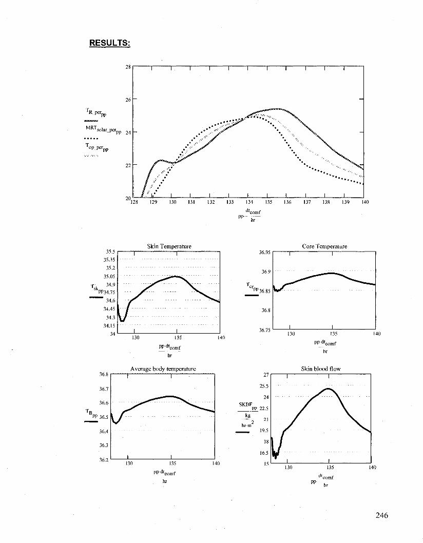
RESULTS:

'R_per PP

MRT solar_per PP 24

op_per. PP

137 138 139 140

PP-comf

hr

Skin Temperature

140

36.95 Core Temperature

T

Average body temperature Skin blood flow

'B PP 36.5

PP-"comf

hr

246

Radiative heat transfer coeff.

•V cl

PP-comf

hr

Convective heat loss from respiration T

PP-"comf

hr

0.17

PP

0.15

Fraction of body mass attributed to skin

dt. P P -

comf

hr

PP

Regulatory sweat rate

pp. comf

hr

Convective and radiative heat loss

dt, pp.

comf

~ h r ~

1

0.8

0.6 S cr p p 0.4

"0.2

-0.4

-0.6

-0.8

-1

• • »

Th .1 • • •

V ,

ermal storage

1 1 1 1 1

"Nl i •A.

• • • • • i i i i i

m core and skin

1 1 1 1 i

••i i i i i 130131132133134135136137138139140141142

dt. PP-

comf

hr

247

'B C =

f 0.194 ^

58.15-

LV

watt 2

m )

(M - Wk) + 36.301 .cold set-point for evaporative regulation zone

l B H -0.347

58.15-watt

(M - Wk) + 36.669 ...hot set-point for evaporative regulation zone

f E •= 0 42-

rsw_req • M - W k - 5 8 . 1 5 -

watt

m2 J Ediff :=

PP PP

max , v ppy

0.06-E„ PP

T S E N S p p := 0.4685-fTB - T B C ) if T B < T g c

V PP -J PP

3 .995rT B - T B C

PP

( T B _ H _ T B _ c ) i f T B C * TB n B H

PP

3.995 + 0.4685fTB - T B H ) if T B H < T B

PP -J ~ PP J

...index of thermal sensation

DISCpp := 0.4685-fTB -TBC) if T B < PP ~ ) PP

B C

47 . /E _ P 1 rsw rsw req PP -

p p p max rsw req c di f f

PP - PR

otherwise

.index of thermal discomfort

lUL- 26.5 if season = 1 , ,„ „ . .„ , . nt

...upper limit of 24 if season = 2 T .op . for Comfort

zone

T L L : = 23 if season = 1 . . J 0 w e r limit of

120.5 if season = 2 T .op . comfort zone

'opjerpp

MRT, solar_per PP

Operative Temperature T

PP-comf

DISC

0.5

-0.5

128 129

2

1.5

1

0.5

0

"0.5

-1.5

DISC and TSENS

1 1 1 1 1 1 1 1 1 1 1

1 1 1 1 I I 130 131 132 133 134 135 136 137 138 139 140

PP: "comf

hr

249

Thermal Comfort Conditions Near Highly Glazed Facades: An ...

Documents

Transcript of Thermal Comfort Conditions Near Highly Glazed Facades: An ...