1

Ginzburg-Landau Theory

Prof. Damian Hampshire Durham University

Cambridge Winter School January 20072

i) Microscopic theory – describes why materials are superconducting

There are two main theories in superconductivity:

ii) Ginzburg-Landau Theory – describes the properties of superconductors in magnetic fields

3

Ginzburg-Landau theory

This is a phenomenological theory, unlike the microscopic BCS theory. Based on a so-called phenomenological order parameter. Not strictly an ab initio theory, but essential for problems concerning superconductors in magnetic fields.G-L was the first theory to explain the difference between Type I and Type II superconductivity, and enable the calculation of two critical fields Hc1 and Hc2.

4

Outline of the LectureGinzburg-Landau theory The two G-L equationsThe basic phenomenology – Type I and Type II superconductorsTime dependent G-L theoryGinzburg-Landau and PinningConclusions

5

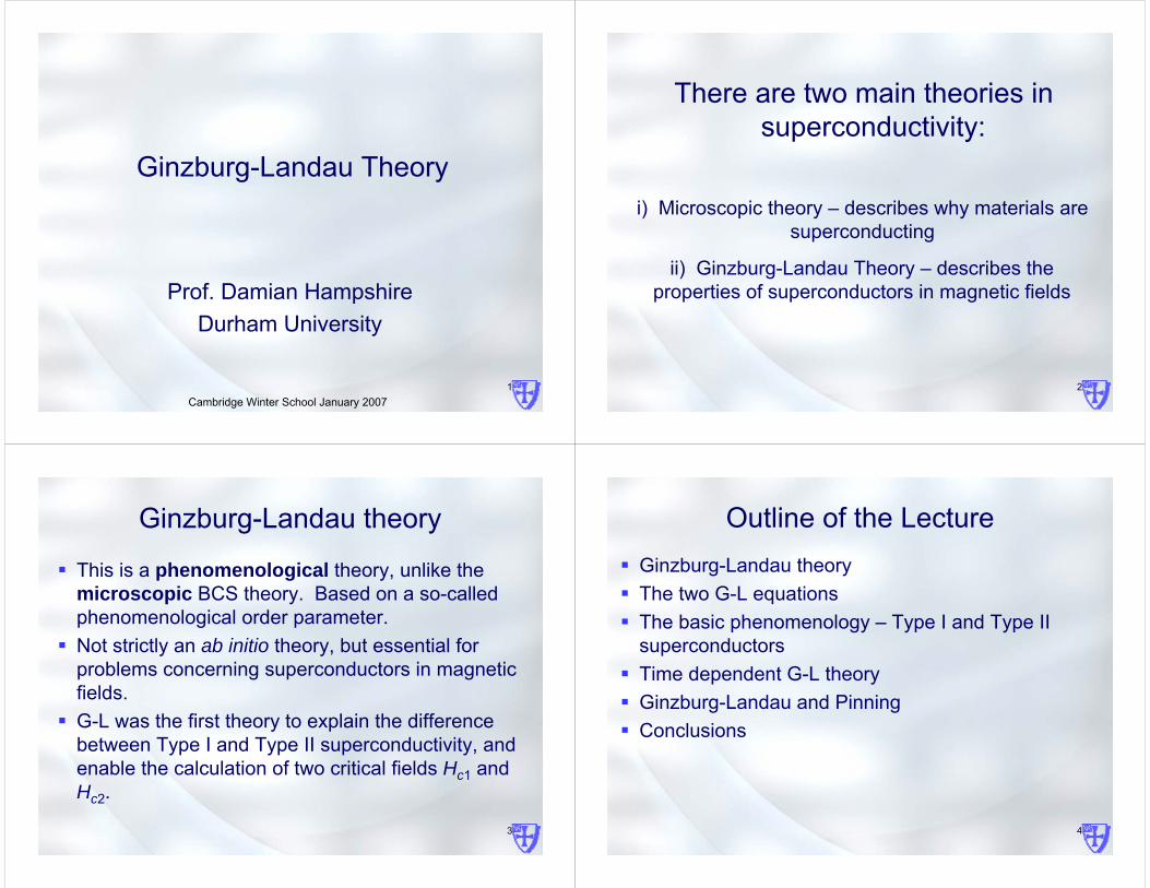
Ginzburg-Landau Theory

2 4 2 - 2e ) + d 1 1f = + + (-i2 2m

α ψ β ψ ψ∇ ∫A H B

Ginzburg and Landau (G-L) postulated a Helmholtz energy density for superconductors of the form:

where α and β are constants and ψ is the wavefunction. α is of the form α’(T-TC) which changes sign at TC

6

The two Ginzburg-Landau Equations

Functional differentiation w.r.t. ψ and A gives the two G-L equations (coupled partial differential equations):

G-L I

G-L II

( ) 02i-21 22 =ΨΨ+Ψ+Ψ−∇ βαAem

( )2

2* *i 4e eJ Am m

= − Ψ ∇Ψ −Ψ∇Ψ − Ψ

7

London Theory – Type I superconductors

The London brothers -

sL Jt

E∂∂

μ= 20λ

sL JB ∧∇μ−= 02λ

*s

*

L enm

0

2

μ=λ

BBL

22 1

λ=∇

Substituting the second London equation into one of Maxwell’s equations we get the Meissner state:

where

8

Magnetisation of superconductors

-Hc

Hc1 Hc Hc2

Type IType II

M

H0

Tc

H0T

Hc1

Hc

Hc2

Meissner

Mixed Normal

The magnetisation (M) of a type I and type II superconductor, with the same Hc as a function of applied magnetic field (Ho). Inset: The phase diagrams of type I and type II superconductors.

9

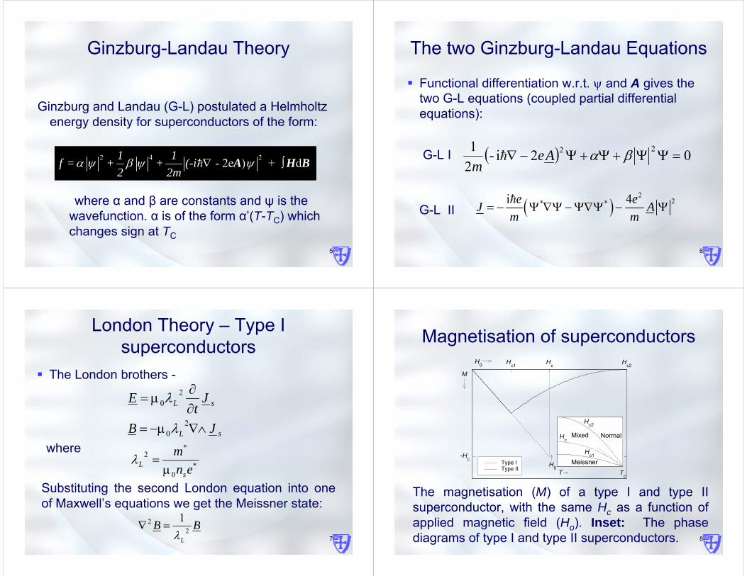
The structure of the fluxon

The order parameter, magnetic field (B) and supercurrent density (JC) as a function of distance (r) from the centre of an isolated vortex (κ ≈ 8). The order parameter squared is proportional to the density of superelectrons.

0

ψ∞

2μ0Hc1

0 ξ λ

Jθ

Bz

Jθ(r)

Bz(r)

r

|ψ(r)|

10

The Mixed state

λ: depth of the current flowd: fluxon – fluxon spacingIf B increases, d decreases.

11

The Mixed State in NbSe2

(a) (b)The hexagonal Abrikosov lattice: (a) contour diagram of the order parameter from Kleiner et al.; the lines also represent contours of B and streamlines of J. (b) Scanning-tunnelling-microscope image of the flux lattice in NbSe2 (1 T, 1.8 K) from Hess et al. the vortex spacing is ~479Å.

12

The Mixed State in Nb

Vortex lattice in niobium – the triangular layout can clearly be seen. (The normal regions are preferentially dark because of the ferromagnetic powder).

13

Flux Quantisation

By considering the persistent current as a wave, phase coherence demands (n: integer) - leads to flux quantisation. k: momentum of the superelectrons.

14

G-L Theory – Type I and Type II superconductors

2 emξ

α=

204em

eβλ

μ α=

Ginzburg-Landau theory predicts that a superconductor should have two characteristic lengths:

Penetration depth

This ratio, κ, distinguishes Type-I superconductors, for which κ ≤ 1/√2, from Type-II superconductors which have higher κ values.

Coherence length

The Ginzburg-Landau parameter λκξ

=

15

Thermodynamic Critical Field, HC

In Type I superconductors HC is the critical field at which superconductivity is destroyed − ψ drops abruptly to zero in a first-order phase transition.At the thermodynamic critical field HC, the Gibbs free energies for superconducting and normal phases are equal. For the superconducting phase B = 0, and for the normal phase ψ = 0

0cH

αμ β

=

16

Lower and upper critical fields

1 ln2C

cH

H κκ

≈

22 1c C CH H Hκ κ≈ ≈

00 2 22cH

φμπξ

=

0cH

αμ β

=

17

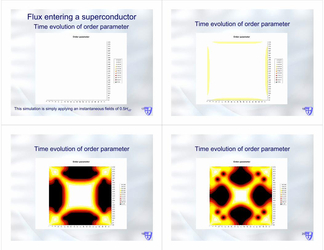
Time evolution of order parameterFlux entering a superconductor

This simulation is simply applying an instantaneous fields of 0.5Hc2. 18

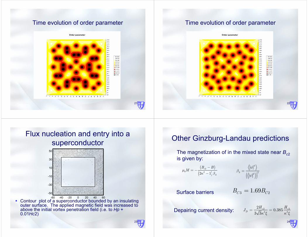
Time evolution of order parameter

19

Time evolution of order parameter

20

Time evolution of order parameter

21

Time evolution of order parameter

22

Time evolution of order parameter

23

Flux nucleation and entry into a superconductor

Contour plot of a superconductor bounded by an insulating outer surface. The applied magnetic field was increased to above the initial vortex penetration field (i.e. to Hp + 0.01Hc2)

-60 -40 -20 0 20 40 60-50

-30

-10

10

30

50

24

Other Ginzburg-Landau predictions

( )( )

20 22 1

c

A

B BMμ

κ β−

= −− ( )

4

22A

ψβ

ψ=

The magnetization of in the mixed state near Bc2is given by:

Surface barriers 3 21.69C CB B=

Depairing current density: 2 222

20.385

3 3c c

DH H

Jκ ξκ ξ

= =

25

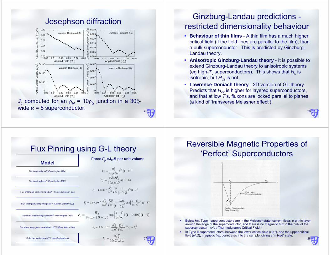
Josephson diffraction

0.00 0.01 0.02 0.03 0.04 0.050.00

0.02

0.04

0.06

0.08

0.10Junction Thickness 0.5ξ

Crit

ical

Cur

rent

Den

sity

(Hc2

/κ2 ξ

)

Applied Field (Hc2)0.00 0.01 0.02 0.03 0.04 0.05

0.000

0.005

0.010

0.015

0.020

0.025

0.030Junction Thickness 1.5ξ

Applied Field (Hc2)

Crit

ical

Cur

rent

Den

sity

(Hc2

/κ2 ξ

)

0.00 0.01 0.02 0.03 0.04 0.050

1x10-3

2x10-3

3x10-3

Junction Thickness 4.5ξ

Applied Field (Hc2)

Crit

ical

Cur

rent

Den

sity

(Hc2

/κ2 ξ

)

0.00 0.01 0.02 0.03 0.04 0.050

1x10-4

2x10-4

3x10-4

4x10-4

Junction Thickness 9.5ξ

Applied Field (Hc2)

Crit

ical

Cur

rent

Den

sity

(Hc2

/κ2 ξ

)

Jc computed for an ρN = 10ρS junction in a 30ξ-wide κ = 5 superconductor.

26

Ginzburg-Landau predictions -restricted dimensionality behaviour

Behaviour of thin films - A thin film has a much higher critical field (if the field lines are parallel to the film), than a bulk superconductor. This is predicted by Ginzburg-Landau theory.Anisotropic Ginzburg-Landau theory - It is possible to extend Ginzburg-Landau theory to anisotropic systems (eg high-Tc superconductors). This shows that Hc is isotropic, but Hc2 is not.Lawrence-Doniach theory - 2D version of GL theory. Predicts that Hc2 is higher for layered superconductors, and that at low T’s, fluxons are locked parallel to planes (a kind of ‘transverse Meissner effect’)

27

Flux Pinning using G-L theory

( )2

1 22 22

0

14

cp

BF b b

Dμ κ= −

( )222

0

31

16c

pB

F b bD

πμ κ

= −

( )( )

52 1 24 2 2

2200 0

2 12.8 10 11

cp

BF b b

ad

πμ κ φ

−= × −−

( )( )

52 3 24 2 2

22 200 0

2 1 0.29 13.9 10 exp 131

cp

B b bF b ba bd

πμ κ φ κ

− ⎛ ⎞− − ⎟⎜= × −⎟⎜ ⎟⎜⎝ ⎠−

( )( )( )

222

2 20 0

1exp 1 0.29 18 3

cp

B bF b b bD a bπμ κ κ

⎛ ⎞− ⎟⎜= − −⎟⎜ ⎟⎜⎝ ⎠−

( )52

23 1.2922

0 0

21.5 10 1cp

BF b bπ

μ κ φ−≈ × −

2 4

3 20 44 6616p p

p

n fF

a C C=

Force Fp =JC.B per unit volume

Collective pinning model34 (Larkin-Ovchinnikov)

Flux shear along grain boundaries in 2D105 (Pruymboom 1988)

Maximum shear strength of lattice27 (Dew-Hughes 1987)

Flux shear past point pinning sites30 (Kramer, Brandt33 C66)

Flux shear past point pinning sites30 (Kramer, Labusch31 C66)

Pinning at surfaces27 (Dew-Hughes 1987)

Pinning at surfaces25 (Dew-Hughes 1974)

Model

28

Reversible Magnetic Properties of ‘Perfect’ Superconductors

Below Hc, Type I superconductors are in the Meissner state: current flows in a thin layer around the edge of the superconductor, and there is no magnetic flux in the bulk of the superconductor. (Hc : Thermodynamic Critical Field.)In Type II superconductors, between the lower critical field (Hc1), and the upper critical field (Hc2), magnetic flux penetrates into the sample, giving a “mixed” state.

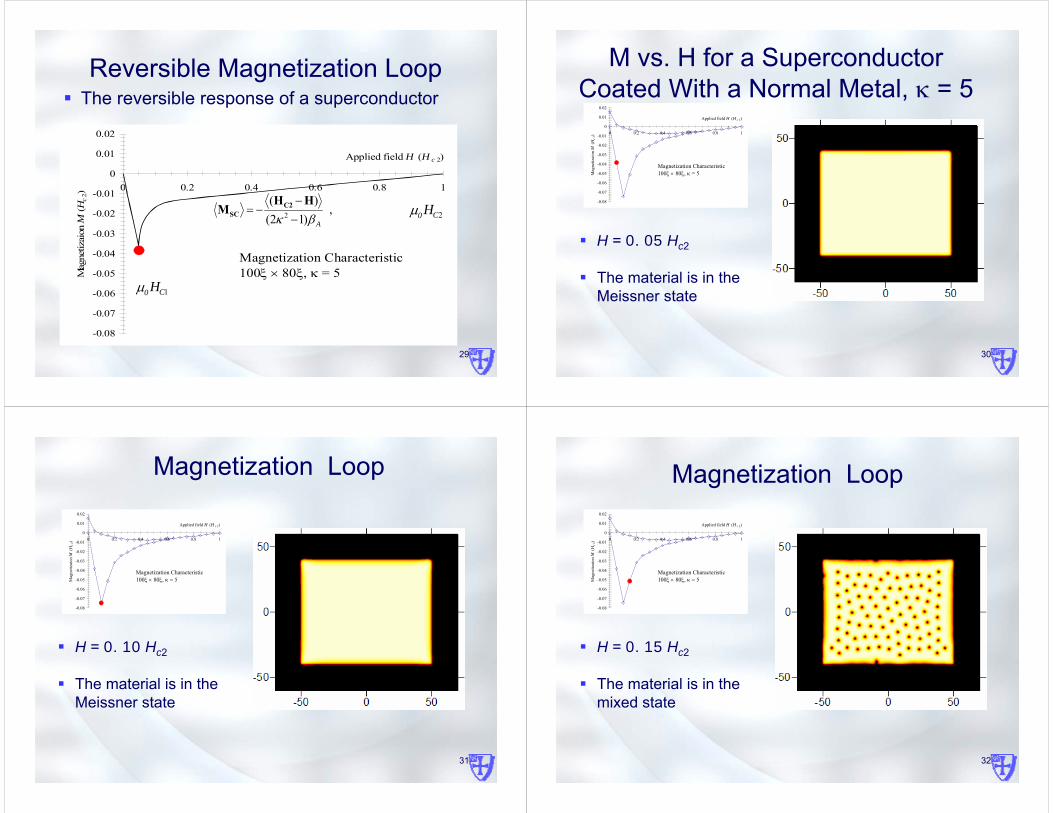
29 -0.08

-0.07

-0.06

-0.05

-0.04

-0.03

-0.02

-0.01

0

0.01

0.02

0 0.2 0.4 0.8 1

Applied field H (H c 2)

Mag

netiz

aion

M(H

c2)

Magnetization Characteristic100ξ × 80ξ, κ = 5

0.6

Reversible Magnetization LoopThe reversible response of a superconductor

,)12(

)(2

Aβκ −−

−=HΗ

M C2SC 2C0 Hμ

1C0 Hμ

30

M vs. H for a Superconductor Coated With a Normal Metal, κ = 5

H = 0.05 Hc2

The material is in the Meissner state

-0.08

-0.07

-0.06

-0.05

-0.04

-0.03

-0.02

-0.01

0

0.01

0.02

0 0.2 0.4 0.6 0.8 1

Applied field H (H c 2)

Mag

netiz

aion

M (H

c2)

Magnetization Characteristic100ξ × 80ξ, κ = 5

31

H = 0.10 Hc2

The material is in the Meissner state

-0.08

-0.07

-0.06

-0.05

-0.04

-0.03

-0.02

-0.01

0

0.01

0.02

0 0.2 0.4 0.6 0.8 1

Applied field H (H c 2)

Mag

netiz

aion

M (H

c2)

Magnetization Characteristic100ξ × 80ξ, κ = 5

Magnetization Loop

32

Magnetization Loop

H = 0.15 Hc2

The material is in the mixed state

-0.08

-0.07

-0.06

-0.05

-0.04

-0.03

-0.02

-0.01

0

0.01

0.02

0 0.2 0.4 0.6 0.8 1

Applied field H (H c 2)

Mag

netiz

aion

M (H

c2)

Magnetization Characteristic100ξ × 80ξ, κ = 5

33

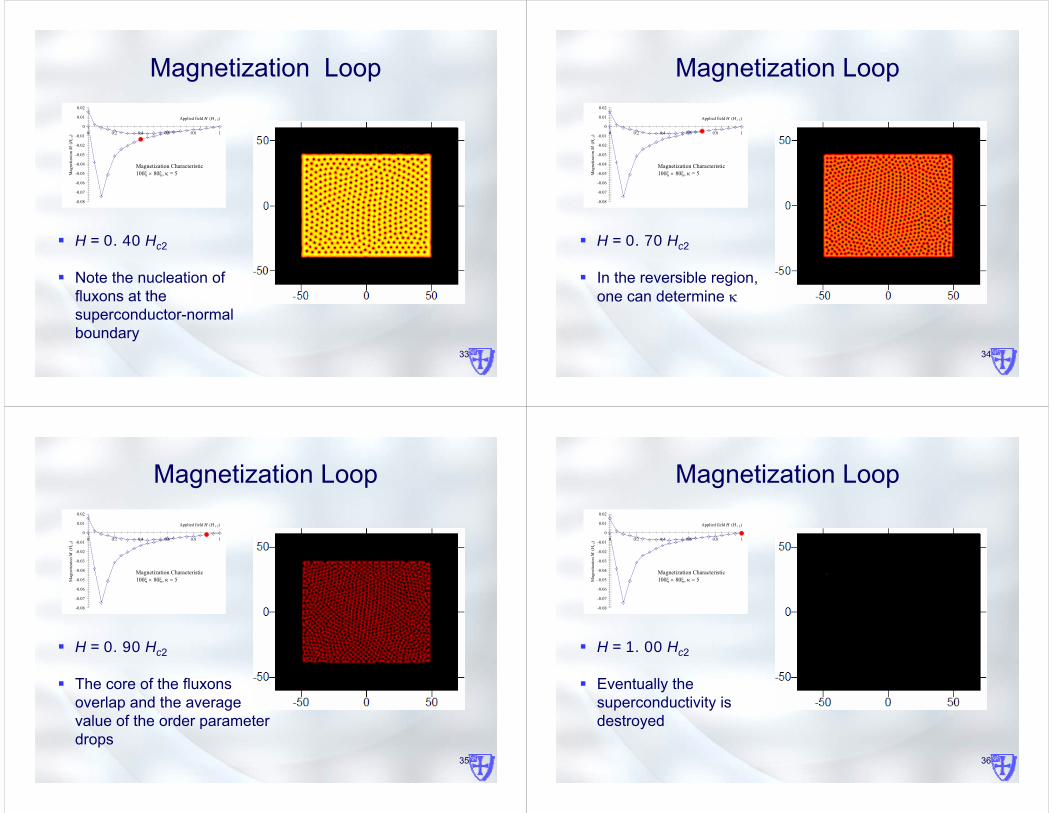
Magnetization Loop

H = 0.40 Hc2

Note the nucleation of fluxons at the superconductor-normal boundary

-0.08

-0.07

-0.06

-0.05

-0.04

-0.03

-0.02

-0.01

0

0.01

0.02

0 0.2 0.4 0.6 0.8 1

Applied field H (H c 2)

Mag

netiz

aion

M (H

c2)

Magnetization Characteristic100ξ × 80ξ, κ = 5

34

Magnetization Loop

H = 0.70 Hc2

In the reversible region, one can determine κ

-0.08

-0.07

-0.06

-0.05

-0.04

-0.03

-0.02

-0.01

0

0.01

0.02

0 0.2 0.4 0.6 0.8 1

Applied field H (H c 2)

Mag

netiz

aion

M (H

c2)

Magnetization Characteristic100ξ × 80ξ, κ = 5

35

Magnetization Loop

H = 0.90 Hc2

The core of the fluxons overlap and the average value of the order parameter drops

-0.08

-0.07

-0.06

-0.05

-0.04

-0.03

-0.02

-0.01

0

0.01

0.02

0 0.2 0.4 0.6 0.8 1

Applied field H (H c 2)

Mag

netiz

aion

M (H

c2)

Magnetization Characteristic100ξ × 80ξ, κ = 5

36

Magnetization Loop

H = 1.00 Hc2

Eventually the superconductivity is destroyed

-0.08

-0.07

-0.06

-0.05

-0.04

-0.03

-0.02

-0.01

0

0.01

0.02

0 0.2 0.4 0.6 0.8 1

Applied field H (H c 2)

Mag

netiz

aion

M (H

c2)

Magnetization Characteristic100ξ × 80ξ, κ = 5

37

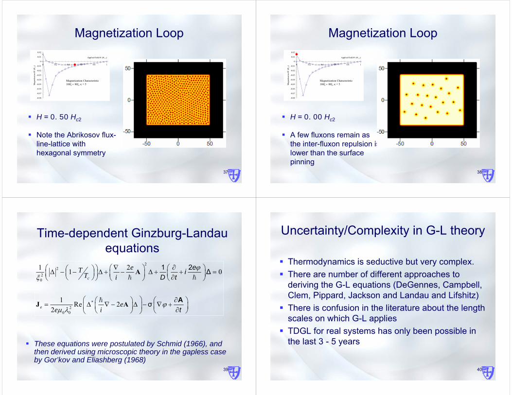
Magnetization Loop

H = 0.50 Hc2

Note the Abrikosov flux-line-lattice with hexagonal symmetry

-0.08

-0.07

-0.06

-0.05

-0.04

-0.03

-0.02

-0.01

0

0.01

0.02

0 0.2 0.4 0.6 0.8 1

Applied field H (H c 2)

Mag

netiz

aion

M (H

c2)

Magnetization Characteristic100ξ × 80ξ, κ = 5

38

Magnetization Loop

H = 0.00 Hc2

A few fluxons remain as the inter-fluxon repulsion is lower than the surface pinning

-0.08

-0.07

-0.06

-0.05

-0.04

-0.03

-0.02

-0.01

0

0.01

0.02

0 0.2 0.4 0.6 0.8 1

Applied field H (H c 2)

Mag

netiz

aion

M (H

c2)

Magnetization Characteristic100ξ × 80ξ, κ = 5

39

Time-dependent Ginzburg-Landau equations

These equations were postulated by Schmid (1966), and then derived using microscopic theory in the gapless case by Gor’kov and Eliashberg (1968)

22

20

*2

0 0

1 21 0

1 Re 22

c

e

eTT i

ee i

ϕξ

ϕμ λ

∇ ∂⎛ ⎞ ⎛ ⎞⎛ ⎞⎛ ⎞Δ − − Δ + − Δ + + =⎜ ⎟⎜ ⎟ ⎜ ⎟ ⎜ ⎟∂⎝ ⎠⎝ ⎠ ⎝ ⎠ ⎝ ⎠

⎛ ⎞ ∂⎛ ⎞ ⎛ ⎞= Δ ∇ − Δ − ∇ +⎜ ⎟ ⎜ ⎟⎜ ⎟ ∂⎝ ⎠ ⎝ ⎠⎝ ⎠

A

J A

1 2 Δ

σ

eiD t

tA

40

Uncertainty/Complexity in G-L theory

Thermodynamics is seductive but very complex. There are number of different approaches to deriving the G-L equations (DeGennes, Campbell, Clem, Pippard, Jackson and Landau and Lifshitz)There is confusion in the literature about the length scales on which G-L appliesTDGL for real systems has only been possible in the last 3 - 5 years

41

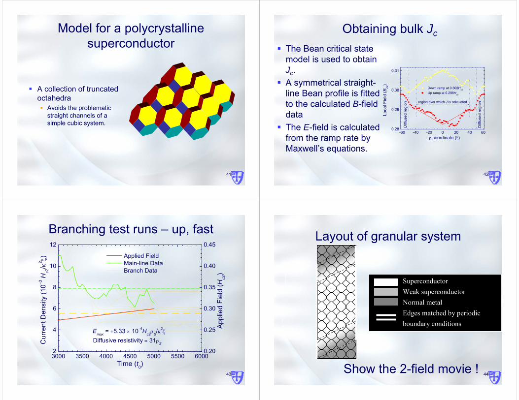
Model for a polycrystalline superconductor

A collection of truncated octahedra

Avoids the problematic straight channels of a simple cubic system.

42

Obtaining bulk Jc

The Bean critical state model is used to obtain Jc. A symmetrical straight-line Bean profile is fitted to the calculated B-field dataThe E-field is calculated from the ramp rate by Maxwell’s equations.

-60 -40 -20 0 20 40 600.28

0.29

0.30

0.31

region over which J is calculated

DIff

used

regi

on

DIff

used

regi

on

Loca

l Fie

ld (B

c2)

y-coordinate (ξ)

Down ramp at 0.302Hc2

Up ramp at 0.298Hc2

43

Branching test runs – up, fast

3000 3500 4000 4500 5000 5500 60002

4

6

8

10

12

Emax = +5.33 × 10−4Hc2ρS/κ2ξ

Diffusive resistivity ≈ 31ρS

Cur

rent

Den

sity

(10−3

Hc2

/κ2 ξ

)

Time (t0)

Applied Field Main-line Data Branch Data

0.20

0.25

0.30

0.35

0.40

0.45

App

lied

Fiel

d (H

c2)

44

Layout of granular system

Superconductor Weak superconductor Normal metal Edges matched by periodic boundary conditions

a

b

x

y

Show the 2-field movie !

45

Time dependant Ginzburg-Landau theory provides the framework for understanding flux pinning

46

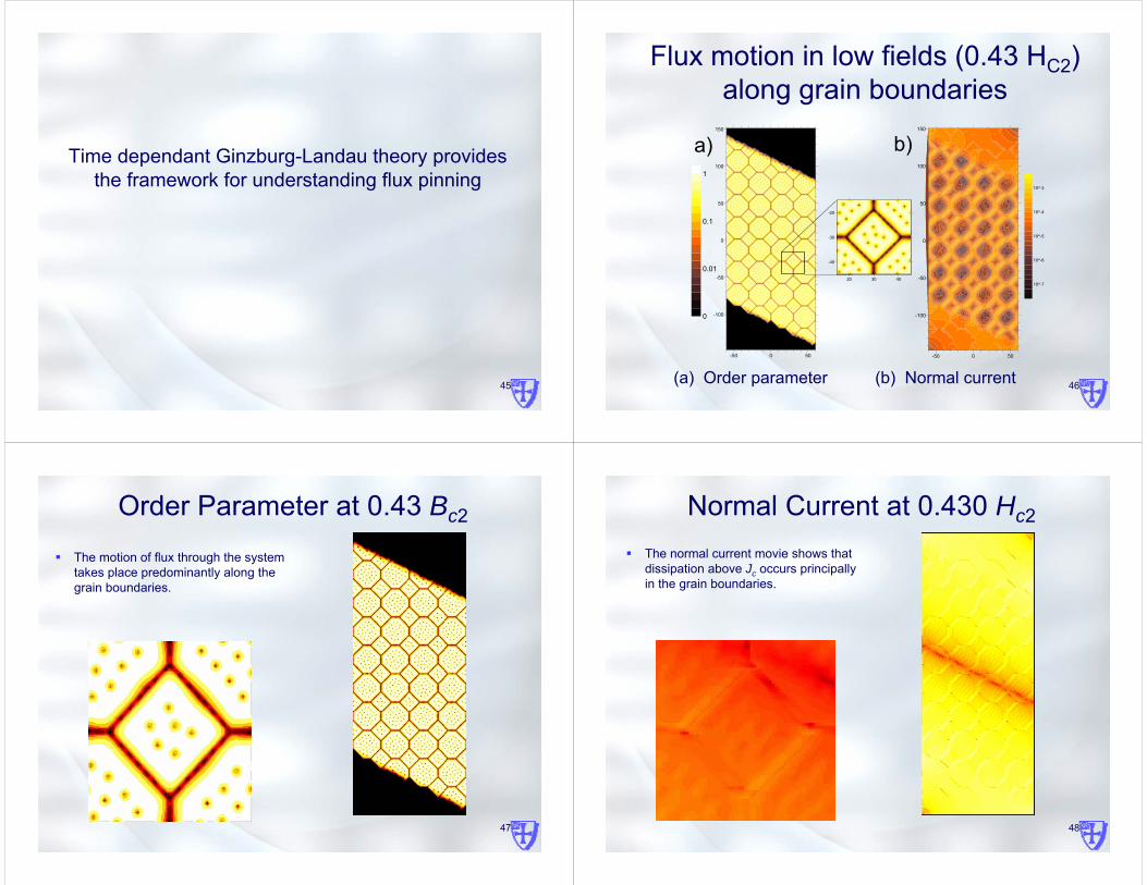
Flux motion in low fields (0.43 HC2) along grain boundaries

(a) Order parameter (b) Normal current-50 0 50

-100

-50

0

50

100

150

20 30 40

-40

-30

-20

a)

-50 0 50

-100

-50

0

50

100

150

b)

0

0.01

0.1

1

10^-7

10^-6

10^-5

10^-4

10^-3

47

Order Parameter at 0.43 Bc2

The motion of flux through the system takes place predominantly along the grain boundaries.

48

Normal Current at 0.430 Hc2

The normal current movie shows that dissipation above Jc occurs principally in the grain boundaries.

49

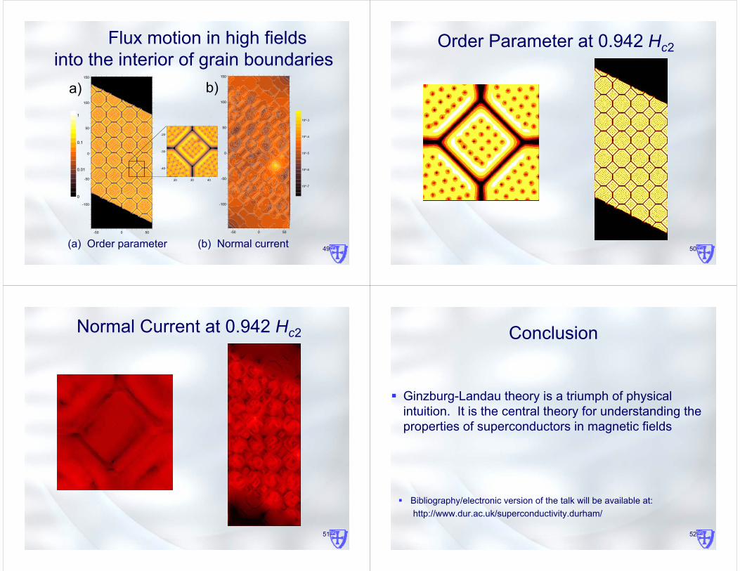
Flux motion in high fields into the interior of grain boundaries

(a) Order parameter (b) Normal current-50 0 50

-100

-50

0

50

100

150

20 30 40

-40

-30

-20

0

0.01

0.1

1

a)

-50 0 50

-100

-50

0

50

100

150

b)

10^-7

10^-6

10^-5

10^-4

10^-3

50

Order Parameter at 0.942 Hc2

51

Normal Current at 0.942 Hc2

52

Conclusion

Ginzburg-Landau theory is a triumph of physical intuition. It is the central theory for understanding the properties of superconductors in magnetic fields

Bibliography/electronic version of the talk will be available at: http://www.dur.ac.uk/superconductivity.durham/