Theory of the Earth - CaltechAUTHORSauthors.library.caltech.edu/25018/16/TOE15.pdf · Anisotropy...

Theory of the Earth Don L. Anderson Chapter 15. Anisotropy Boston: Blackwell Scientific Publications, c1989 Copyright transferred to the author September 2, 1998. You are granted permission for individual, educational, research and noncommercial reproduction, distribution, display and performance of this work in any format. Recommended citation: Anderson, Don L. Theory of the Earth. Boston: Blackwell Scientific Publications, 1989. http://resolver.caltech.edu/CaltechBOOK:1989.001 A scanned image of the entire book may be found at the following persistent URL: http://resolver.caltech.edu/CaltechBook:1989.001 Abstract: Anisotropy is responsible for the largest variations in seismic velocities; changes in the preferred orientation of mantle minerals, or in the direction of seismic waves, cause larger changes in velocity than can be accounted for by changes in temperature, composition or mineralogy. Therefore, discussions of velocity gradients, both radial and lateral, and chemistry and mineralogy of the mantle must allow for the presence of anisotropy. Anisotropy is not a second-order effect. Seismic data that are interpreted in terms of isotropic theory can lead to models that are not even approximately correct. On the other hand a wealth of new information regarding mantle mineralogy and flow will be available as the anisotropy of the mantle becomes better understood.

http://resolver.caltech.edu/CaltechBOOK:1989.001

http://resolver.caltech.edu/CaltechBook:1989.001

Anisotropy

And perpendicular now and now transverse, Pierce the dark soil and as they pierce and pass Make bare the secrets of the Earth's deep heart.

A nisotropy is responsible for the largest variations in seismic velocities; changes in the preferred orienta-

tion of mantle minerals, or in the direction of seismic waves, cause larger changes in velocity than can be accounted for by changes in temperature, composition or mineralogy. Therefore, discussions of velocity gradients, both radial and lateral, and chemistry and mineralogy of the mantle must allow for the presence of anisotropy. Anisot- ropy is not a second-order effect. Seismic data that are interpreted in terms of isotropic theory can lead to models that are not even approximately correct. On the other hand a wealth of new information regarding mantle mineralogy and flow will be available as the anisotropy of the mantle becomes better understood.

INTRODUCTION

The Earth is usually assumed to be isotropic to the propagation of seismic waves. It should be stressed that this assumption is made for mathematical convenience. The fact that a large body of seismic data can be satisfactorily modeled with this assumption does not prove that the Earth is isotropic. There is often a direct trade-off between anisotropy and heterogeneity. An anisotropic structure can have characteristics, such as travel times and dispersion curves, that are identical, or similar, to a different isotropic structure. A layered solid, for example, composed of isotropic layers that are thin compared to a seismic wavelength will behave as an anisotropic solid. The velocity of propagation depends on direction. The effective long-wavelength elastic constants depend on the thicknesses and elastic properties of the individual layers. The reverse is also true: An aniso-

tropic solid with these same elastic constants can be modeled exactly as a stack of isotropic layers. The same holds true for an isotropic solid permeated by oriented cracks or aligned inclusions. This serves to illustrate the trade-off between heterogeneity and anisotropy. Not all anisotropic structures, however, can be modeled by laminated solids.

The crystals of the mantle are generally anisotropic, and rocks from the mantle show that these crystals exhibit a high degree of alignment. There is also evidence that crystal alignment is uniform over large areas of the upper mantle. At mantle temperatures, crystals tend to be easily recrystallized and aligned by the prevailing stress and flow fields.

The effects of anisotropy are often subtle and, if unrec- ognized, are usually modeled as inhomogeneities, for example, as layering or gradients. The most obvious manifes- tations of anisotropy are:

Shear-wave birefringence-the two polarizations of S-waves arrive at different times;

Azimuthal anisotropy-the arrival times, or apparent velocities of seismic waves at a given distance from an event, depend on azimuth;

An apparent discrepancy between Love waves and Ray- leigh waves.

Even these are not completely unambiguous indicators of anisotropy. Effects such as P-S conversion, dipping inter- faces, attenuation, and density variations must be properly taken into account.

There is now a growing body of evidence that much of the upper mantle may be anisotropic to the propagation of seismic waves. The early evidence was the discrepancy be-

tween dispersion of Rayleigh waves and Love waves (An- derson, 1961, 1967; Harkrider and Anderson, 1962) and the azimuthal dependence of oceanic Pn velocities (Hess, 1964; Raitt and others, 1969, 1971). Azimuthal variations have now been documented for many areas of the world, and the Rayleigh-Love discrepancy is also widespread. Shear-wave birefringence, a manifestation of anisotropy, has also been reported. The degree of anisotropy varies but is typically about 5 percent. It is not known to what depth the anisotropy extends, but there is abundant evidence for it at depths shallower than 200 krn.

It has been known for some time that the discrepancy between mantle Rayleigh and Love waves could be explained if the vertical P and S velocities in the upper mantle were 7-8 percent less than the horizontal velocities (Ander- son, 1967). Models without an upper-mantle low-velocity zone, such as the Jeffreys model, could satisfy the dispersion data if the upper mantle was anisotropic. The surface- wave data, which are sensitive to the properties of the upper mantle, imply a low-velocity zone if the mantle is assumed to be isotropic. The Love-Rayleigh discrepancy has sur- vived to the present, and average Earth models have been proposed that have SV in the upper mantle less than SH by about 3 percent. Some early models, however, were based on separate isotropic inversions of Love and Rayleigh waves (pseudo-isotropic inversions) and therefore did not indicate the true anisotropy. There is a trade-off between anisotropy and structure. In particular, the very low upper- mantle average shear velocities, 4.0-4.2 kmis, found by many isotropic and pseudo-isotropic inversions, are not a characteristic of models resulting from full anisotropic inversion. The P-wave anisotropy also makes a significant contribution to Rayleigh wave dispersion. This has been ignored in many inversion attempts.

Since intrinsic anisotropy requires both anisotropic crystals and preferred orientation, the anisotropy of the mantle contains information about the mineralogy and the flow. For example, olivine, the most abundant upper-mantle mineral, is extremely anisotropic for both P-wave and S-wave propagation. It apparently is easily oriented by the ambient stress or flow field. Olivine-rich outcrops show a consistent preferred orientation over large areas. In general, the seismically fast axes of olivine are in the plane of the flow with the a axis, the fastest direction, pointing in the direction of flow. The b axis, the minimum velocity direction, is generally normal to the flow plane. Pyroxenes are also very anisotropic. The petrological data are summarized in Peselnick and others (1974) and Christensen and Salis- bury (1979).

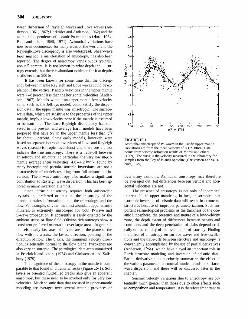
The magnitude of the anisstropy in the mantle is comparable to that found in ultramafic rocks (Figure 15- 1). Soft layers or oriented fluid-filled cracks also give an apparent anisotropy, but these need to be invoked only for very low velocities. Much seismic data that are used in upper-mantle modeling are averages over several tectonic provinces or

I I I I I I I I

40 80 120 160 200 240 280 320 2 AZIMUTH

FIGURE 15-1 Azimuthal anisotropy of Pn waves in the Pacific upper mantle. Deviations are from the mean velocity of 8.159 km/s. Data points from seismic-refraction results of Morris and others (1969). The curve is the velocity measured in the laboratory for samples from the Bay of Islands ophiolite (Christensen and Salis- bury, 1979).

over many azimuths. Azimuthal anisotropy may therefore be averaged out, but differences between vertical and horizontal velocities are not.

The presence of anisotropy is not only of theoretical interest. If the upper mantle is, in fact, anisotropic, then isotropic inversion of seismic data will result in erroneous structures because of improper parameterization. Such important seismological problems as the thickness of the oceanic lithosphere, the presence and nature of a low-velocity zone, the depth extent of differences between oceans and continents and the deep penetration of slabs depend criti- cally on the validity of the assumption of isotropy. Finding the effect of anisotropy on surface waves and free oscillations and the trade-offs between structure and anisotropy is conveniently accomplished by the use of partial derivatives (Anderson, 1964), which have played an important role in Earth structure modeling and inversion of seismic data. Partial-derivative plots succinctly summarize the effect of the various parameters on normal-mode periods or surface- wave dispersion, and these will be discussed later in the chapter.

Seismic velocity variations due to anisotropy are po- tentially much greater than those due to other effects such as composition and temperature. It is therefore important to

understand anisotropy well before one attempts to infer chemical, mineralogical and temperature variations from seismic data. A change in preferred orientation with depth or from one tectonic region to another can be easily misinterpreted.

The study of mantle anisotropy to infer mineralogy and flow is an example of how many disciplines are involved in the recognition and solution of a major problem in geophysics. The mineral physicist measures the single-crystal elastic constants of mantle candidate minerals. The field ge- ologist maps rock fabrics and notices the orientation of minerals relative to bedding planes, dikes and sills. The experimental tectonophysicist deforms rocks and single crystals in the laboratory in order to understand the processes of creep, slip and recrystallization. The thermodynamicist de- velops theories of crystal behavior in non-hydrostatic stress fields. Mathematicians derive the theory for wave propagation in anisotropic media. Seismologists develop a variety of methods for mapping anisotropy in the mantle. Convec- tion modelers calculate flow and stress fields for a range of assumptions about flow in the mantle. Only when all of these elements are in place can one completely interpret seismic data in terms of mantle convection. The study of seismic anisotropy is a rich and vigorous field for a variety of subdisciplines in geology and geophysics.

ORIGIN OF MANTLE ANISOTROPY

Nicholas and Christensen (1987) elucidated the reason for strong preferred crystal orientation in deformed rocks. First, they noted that in homogeneous deformation of a specimen composed of minerals with a dominant slip system, the preferred orientations of slip planes and slip directions coincide respectively with the orientations of the flow plane and the flow line. Simple shear in a crystal rotates all the lines attached to the crystal except those in the slip plane. This results in a bulk rotation of crystals so that the slip planes are aligned, as required to maintain contact between crystals. The crystal reorientations are not a direct result of the applied stress but are a geometrical require- ment. Bulk anisotropy due to crystal orientation is therefore induced by plastic strain and is only indirectly related to stress. The result, of course, is also a strong anisotropy of the viscosity of the rock, and presumably attenuation, as well as elastic properties. This means that seismic techniques can be used to infer flow in the mantle. It also means that mantle viscosity inferred from postglacial rebound is not necessarily the same as that involved in plate tectonics and mantle convection.

Peridotites from the upper mantle display a strong preferred orientation of the dominant minerals, olivine and orthopyroxene. They exhibit a pronounced acoustic-wave

anisotropy that is consistent with the anisotropy of the con- stituent minerals and their orientation. In igneous rocks preferred orientation can be caused by grain rotation, recrystallization in a nonhydrostatic stress field or in the presence of a thermal gradient, crystal setting in magma chambers, flow orientation and dislocation-controlled slip. Macroscopic fabrics caused by banding, cracking, sill and dike injection can also cause anisotropy.

Plastic flow induces preferred orientations in rock- forming minerals. The relative roles of deviatoric stresses and plastic strain have been long debated. In order to assure continuity of a deforming crystal with its neighbors, five independent degrees of motion are required (the Von Mises criterion). This can be achieved in a crystal with the acti- vation of five independent slip systems or with a combination of fewer slip systems and other modes of deformation. In silicates only one or two slip systems are activated under a given set of conditions involving a given temperature, pressure and deviatoric stresses. The homogeneous deformation of a dominant slip system and the orientation of slip planes and slip directions tend to coincide with the flow plane and the flow direction (Nicholas and Christen- sen, 1987).

Mantle peridotites typically contain more than 65 percent olivine and 20 precent orthopyroxene. The high-V, direction in olivine (Figure 15-2) is along the a axis [100], which is also the dominant slip direction at high temperature. The lowest V, crystallographic direction is [OlO], the b direction, which is normal to a common slip plane. Thus, the V, pattern in olivine aggregates is related to slip orientations. There is no such simple relationship with the V, anisotropy and, in fact, the S-wave anisotropy of peridotites is small.

Orthopyroxenes also have large P-wave anisotropies and relatively small S-wave anisotropies, and have the prin- cipal V, directions related to the slip system. The high-V, direction coincides with the [loo] pole of the unique slip plane and the intermediate V, crystallographic direction coincides with the unique [OO13 slip line (Figure 15-2). In natural peridotites the preferred orientation of olivine is more pronounced than the other minerals. Olivine is apparently the most ductile and easily oriented upper-mantle mineral, and therefore controls the seismic anisotropy of the upper mantle. The anisotropy of /3-spinel, a high-pressure form of olivine that is expected to be a major mantle component below 400 km, is also high. The y-spinel form of olivine, stable below about 500 km, is much less anisotropic. Recrystallization of olivine to spinel forms can be expected to yield aggregates with preferred orientation but with perhaps less pronounced P-wave anisotropy. P-spinel has a strong S-wave anisotropy (24 percent variation with direction, 16 percent maximum difference between polarizations). The fast shear directions are parallel to the slow P-wave directions, whereas in olivine the fast S-directions correspond to intermediate P-wave velocity directions.

OLIV INE /A$@5 ORTHOPYROXENE

O L I V I N E ORTHOPYROXE NE

FIGURE 15-2 Olivine and orthopyroxene orientations within the upper mantle showing compressional velocities for the three crystallographic axes, and compressional and shear velocities in the olivine a-c plane and orthopyroxene b-c plane (after Christensen and Lundquist, 1982).

Orthopyroxene transforms to a cubic garnet-like structure that is stable over much of the transition region part of the upper mantle. This mineral, majorite, is expected to be relatively isotropic. Therefore, most of the mantle between 400 and 650 km depth is expected to have relatively low anisotropy, with the anisotropy decreasing as olivine transforms successively to P-spinel and y-spinel. At low temperatures, as in subduction zones, the stable form of pyroxene is an ilmenite-type structure that is extremely anisotropic. Thus, the deep part of slabs may exhibit pronounced anisotropy, a property that could be mistaken for deep slab penetration in certain seismic experiments.

Different slip systems in olivine are activated at different temperatures (Avt Lallement and Carter, 1970; Carter, 1976; Nicholas and Pokier, 1976). At very high temperature olivine slips essentially with a single slip system and peridotites develop very strong fabrics. Although it is the anisotropy of individual crystals and their degree of orientation that controls the seismic anisotropy, it is dislocation physics and geometric constraints, combined with external

variables such as the stress, flow and temperature, that ul- timately control the degree of orientation. Thus, seismic data have the potential to infer not only mineralogy but also present and paleostress fields.

Petrofabric studies combined with field studies on ophiolite harzburgites give the following relationships:

Olivine c axes and orthopyroxene b axes lie approximately parallel to the inferred ridge axis in a plane parallel to the Moho discontinuity.

The olivine a axes and the orthopyroxene c axes align subparallel to the inferred speading direction.

The olivine b axes and the orthopyroxene a axes are approximately perpendicular to the Moho.

These results indicate that the compressional velocity the vertical direction increases with the orthopyroxene

content, whereas horizontal velocities and anisotropy decrease with increasing orthopyroxene content.

The maximum compressional wave velocity in orthopyroxene (along the a axis) parallels the minimum (b axis) velocity of olivine. For olivine b axis vertical regions of the mantle, as in ophiolite peridotites, the vertical P-velocity increases with orthopyroxene content. The reverse is true for other directions and for average properties. Appreciable shear-wave birefringence is expected in all directions even if the individual shear velocities do not depend much on azimuth. The total P-wave variation with azimuth in olivine- and orthopyroxene-rich aggregates is about 4 to 6 percent, while the S-waves only vary by 1 to 2 percent (Figure 15-3). The difference between the two shear-wave polarizations, however, is 4 to 6 percent. The azimuthal variation of S-waves can be expected to be hard to measure because the maximum velocity difference occurs over a small angular difference and because of the long-wavelength nature of shear waves. However, Tanimoto and Anderson (1984) measured azimuthal variations of surface-wave velocities that are comparable to the above predictions. The azimuthal variation of Rayleigh waves involves the azimuthal variation of both the P-waves and the SV-waves. The above relations between P-wave and S-wave anisotropy are not

FIGURE 15-3 Equal area projection of V, and two shear velocities measured on samples of peridotite. Dashed line is vertical direction, solid great circle is the horizontal (after Christensen and Salisbury, 1979).

general and should not be applied to deeper parts of the mantle. In particular, the shear-wave anisotropy in the ilmenite structure of pyroxene, expected to be important in the deeper parts of subducted slabs, is quite pronounced and bears a different relationship to the P-wave anisotropy than that in peridotites. One possible manifestation of slab anisotropy is the variation of travel times with take-off angle from intermediate- and deep-focus earthquakes. Fast in- plane velocities, as expected for oriented olivine and probably spinel and ilmenite, may easily be misinterpreted as evidence for deep slab penetration. The mineral assem- blages in cold slabs are also different from the stable phases in normal and hot mantle. The colder phases are generally denser and seismically fast. Anisotropy and isobaric phase changes have been ignored in most studies purporting to show deep slab penetration into the lower mantle. There is a complete trade-off, however, between the length of a high- velocity slab and its velocity contrast and anisotropy.

ANISOTROPY OF CRYSTALS

Because of the simplicity and availability of the micro- scope, the optical properties of minerals receive more at- tention than the acoustic properties. It is the acoustic or ultrasonic properties, however, that are most relevant to the interpretation of seismic data. Being crystals, minerals exhibit both optical and acoustic anisotropy. Aggregates of crystals, rocks, are also anisotropic and display fabrics that can be analyzed in the same terms used to describe crystal symmetry. Tables 15-1, 15-2 and 15-3 summarize the acoustic anisotropy of some important rock-forming minerals. Pyroxenes and olivine are unique in having a greater P-wave anisotropy than S-wave anisotropy. Spinel and garnet, cubic crystals, have low P-wave anisotropy. Hexagonal crystals, and the closely related class of trigonal crystals, have high shear-wave anisotropies. This is perti- nent to the deeper part of cold subducted slabs in which the trigonal ilmenite form of pyroxene may be stable. Deep- focus earthquakes exhibit a pronounced angular variation in both S- and P-wave velocities and strong shear-wave birefringence. Cubic crystals do not necessarily have low shear- wave anisotropy. The major minerals of the shallow mantle are all extremely anisotropic. P-spinel and clinopyroxene are stable below 400 km, and these are also fairly anisotropic. Below 400 krn the major mantle minerals at high temperature, y-spinel and, probably, garnet-majorite are less anisotropic. At the temperatures prevailing in subduction zones, the cold high-pressure forms of orthopyroxene, clinopyroxene and garnet are expected to give high velocities and anisotropies. If these are lined up, by stress or flow or recrystallization, then the slab itself will be anisotropic. This effect will be hard to distinguish from a long isotropic slab, if only sources in the slab are used.

TABLE 15-1 Anisotropic Properties of Rock-Forming Minerals

Max S Anisotropy ' P direction Direction1 (percent)

Mineral Symmetry Max. Min. Polarization P S

Olivine Orthorhombic [loo] [Olol 45'1 135' * 25 22 Garnet Cubic [Ooll -50" * [I101 I [I101 0.6 1 Orthopyroxene Orthorhombic [loo] [Olol [OlO] I [OOl] 16 16 Clinopyroxene Monoclinic [Ooll [loll [oil] 1 [oil] 21 20 Muscovite Monoclinic [1101 [Ooll [OlO] I [loo] 58 85 Orthoclase Monoclinic [Olol [loll [Oll] / [Oli] 46 63 Anorthite Triclinic [Olol [loll [Oll] / [Oli] 36 52 Rutile Tetragonal [Ooll [loo] [loo] I [OlO] 28 68 Nepheline Hexagonal [oo 1 1 [loo] [oil] 1 [oil] 24 32 Spinel Cubic [loll [Ooll [loo] / [OlO] 12 68 P-Mg2Si0, Orthorhombic [Olol [OOl] - 16 14

Babuska (1981), Sawamoto and others (1984). *Relative to [OOl]. +mm, - v ~ ~ ~ Y v ~ ~ ~ ~ ~ X 100.

The elastic properties of simple oxides and silicates are predominantly controlled by the oxygen anion framework, especially for hexagonally close-packed and cubic close- packed structures, but also by the nature of the cations oc- curring within the oxygen interstices. Corundum (Al,O,) consists of a hexagonal close-packed array of oxygen ions (radius 1.4& into which the smaller aluminum ions (0.54W) are inserted in interstitial positions. Forsterite (Mg2Si04) consists of a framework of approximately hexagonal close-packed oxygen ions with the Mg2+ cations (0.72W) occupying one-half of the available octahedral sites (sites surrounded by six oxygen ions) and the Si4+ cations (0.26A) occupying one-eighth of the available tetrahedral sites (sites surrounded by four oxygens). The packing of the oxygens depends on the nature of the cations.

Leibfried (1955) calculated the elastic constants for hexagonal close-packed (h.c.p.) and face-centered cubic (f.c.c.) structures from a central force model in which only the nearest neighbor interactions are considered. The elastic

TABLE 15-2 Elastic Constants of Cubic Crystals

C11 C 12 C44 P Mineral (Mbar) (g/cm3)

Garnet 2.966 1.085 0.916 3.705 y-Mg,Si04 3.27 1.12 1.26 3.559 MgO 2.97 0.95 1 .56 3.580 MgAlzO, 2.82 1.55 1.54 3.578

Chang and Barsch (1969), Liu and others (1975), Suzuki and Anderson (1983), Weidner and others (1984).

constants C are expressed in terms of the bulk modulus K:

The coefficients aij are numbers that depend on the crystal symmetry only. The bulk modulus is

where f is the force constant and d is the nearest neighbor distance. The coefficients a, are

and

This theoretical model refers to the static lattice and ignores thermal effects. This model was tested against experimental data by Gieske and Barsch (1968). Table 15-4 tabulates results for the theoretical model and several crystals that exhibit hexagonal or cubic packing of the oxygen anions. The moduli are normalized to the bulk modulus; the pressure derivatives are normalized to the pressure derivative of the bulk modulus, K t . The simple theoretical model, ignor- ing cations, does a fairly good job of predicting the relative

TABLE 15-3 Elastic Constants of Orthorhombic, Trigonal, Tetragonal and Monocliniic Crystals

Mineral C11 C22 C 33 CM C 55 Cs6 C12 C13 C 23 C 14 C ~ 5

a-Mg ,Si4 3.28 /3-Mg,SiO, 3.60 y-Mg2Si04* 3.46 Bronzite 2.30

Diopside 2.23

Orthorhombic 0.66 0.81 0.81 1.12 1.18 0.98 1.26 1.26 1.08 0.83 0.76 0.79

Trigonal 1.06 (1.06) (1.52"") 1.47 (1.47) (1.67**)

Tetragonal 2.52 (2.52) 3.02

Monoclinic 0.74 0.67 0.66

c , , = 0.17 c,, = 0.43 c,, = 0.073

Kumazawa (1969), Levien and others (1979), Weidner and others (1984).

*Rotated 45" about c axis (three independent constants). 84.5 percent MgSiO,.

( ) Not independent of other entries.

sizes of the elastic constants and even, in some cases, the pressure derivatives. The ratio KIG for the theoretical models is about 1.7, which corresponds to a Poisson's ratio of 0.25. In real crystals the KIG ratio depends on the nature of the cations, coordination, the radius ratios (rCationlrani,,), the valencies and the covalencies. Transition ions cause a large increase in KIG.

THEORY OF ANISOTROPY

In an isotropic elastic solid there are two types of elastic waves. One type is variously called compressional, longitudinal or dilational and is characterized by particle motion in the direction of propagation. The second type of wave-the transverse, shear or distortional-has particle motion in a plane normal to the direction of propagation. For anisotropic media waves are neither purely longitudinal nor transverse, except in certain directions. The particle displacement has components both along and transverse to the direction of propagation. In an anisotropic medium the velocity of shear waves depends not only on direction but also on the polarization. In general, there are two shear waves that propagate with different velocities. This is known as shear-wave birefringence. Since particle motions are no longer simply related to ray directions or wave fronts, the waves are called quasi-P, quasi-longitudinal or quasi- transverse waves. I will continue, however, to refer to these as P-waves and S-waves since the faster, or primary,

waves are P-like in their particle motions; the secondary or slower waves are still S-like.

Stress and strain in a solid body can each be resolved into six components: three extensional and three shearing. According to Hooke's law, each stress component can be expressed as a linear combination of the strain components and vice versa. For the most anisotropic material there are 21 constants of proportionality, the elastic constants or moduli or stiffnesses. As the symmetry increases, the number of elastic constants decreases. For an isotropic body, only two moduli are independent. For small displacements the stresses, Ti, are proportional to the strains, S,:

where c , , , for example, is an elastic constant expressing the proportionality between the T I stress and the S, strain. Since the internal energy U is a perfect differential,

There are at most 21 elastic constants for the most un- symmetrical crystal, a triclinic crystal. For an isotropic solid the constants are independent of the choice of axes and reduce to two: These are the Lam6 constants A and p,

TABLE 15-4 Elastic Constants (a , = c , lK) of Hexagonal Close Packed (h.c.p.) and Face Centered Cubic (f.c.c.) Arrays of Oxygen Ions Compared with Elastic Constants and Pressure Derivatives ( c ; lKf ) of Oxides and Silicates

Hexagonal A 1 A MgSiO,(il) Mg ,SiO,(ol)

ij a y cglK c,;1K1 cglK c , /K c,;lK1

11 1.81 1.97 1.79 2.23 1.86 1.59 22 1.81 1.97 1.79 2.23 1.58 1.64 33 2.00 1.98 1.58 1.80 2.59 1.84 44 0.50 0.58 0.80 0.50 0.64 0.72 55 0.50 0.58 0.80 0.50 0.64 0.55 66 0.56 0.66 0.61 0.72 0.53 0.69 12 0.69 0.65 0.57 0.79 0.57 0.58 13 0.50 0.44 0.65 0.33 0.54 0.67 23 0.50 0.44 0.65 0.33 0.52 0.70 14 0.00 -0.09 0.02 -0.13 25 0.00 0.00

Cubic MgO(rs) A1 2Mg04(s~) SmAlO,(pv)

i j ag cglK cL>lK1 c,,lK c,;IK1 c,;IKf

11 1 S O 1.85 2.1 1.44 1.13 1.69 33 1.50 1.85 2.1 1.44 1.13 1.69 12 0.75 0.58 0.44 0.73 0.92 0.74 13 0.75 0.58 0.44 0.73 0.92 0.63 44 0.75 0.97 0.26 0.76 0.21 0.75 66 0.75 0.97 0.26 0.76 0.21 0.63

- --

Cubic Garnet SrTiO,(pv)

i j a B cylK chlK' c,lK c,;lK'

11 1.50 1.74 1.43 1.85 1.78 33 1.50 1.74 1.43 1.85 1.78 12 0.75 0.63 0.78 0.60 0.61 13 0.75 0.63 0.78 0.60 0.61 44 0.75 0.54 0.30 0.72 0.22 66 0.75 0.54 0.30 0.72 0.22

and all other constants are zero. The Lam6 constant p is the same as the rigidity or shear modulus, G.

The bulk modulus, K, is the ratio between an applied hydrostatic pressure P and the fractional change in volume A (= s, + s, + S,):

K = PlA = A + ( 2 1 3 ) ~

P = T1 = T2 = T3

T, = T5 = T6 = 0

S, = S2 = S3 = A/3 = -P/(3A + 2p)

Young's modulus, E, is the ratio between an applied longitudinal stress and the longitudinal extension when the lateral surfaces are stress-free as in a bar:

E = p(3A + 2p)/(A + p)

Poisson's ratio, u, is the negative of the ratio between the lateral contraction and the longitudinal extension:

u = A/[2(A + p)]

When the strains are expressed in terms of the stresses,

Si = s..T. 11 I

S . . = S . . 11 11

For the isotropic case,

s l l = sZ2 = s~~ = 1/E

s12 = S13 = SZ3 = - u s I 1 = - u l E

su = S55 = S66 = 1 /p

The S, are called compliances.

The wave equation is usually written in terms of strains and elastic constants. Christoffel showed that the equations of motion could be written in terms of the displacements (u,v,w) and a series of moduli, A,, which are functions of the elastic constants or stiffnesses c, and direction cosines (l,m,n) of the normal to the plane wave:

a2 u a2 u a2 v a2w P 7 = A l l + A12 - + A13

at as2 as2 as2

where p is density, t is time, and

A,, = l2cIl + m2c66 + n2cS5 + 2rnncs6

+ 2nk,, + 21mc16

The particle velocity 6 of a point on the surface has direc-

A33 = k2cs5 + m2c, + n 2 ~ 3 3 + 2 r n n ~ ~ ~

+ 2nlc3, + 21mc45

The solution for an isotropic medium indicates three waves propagated, but it is only in special cases that the particle motions will be perpendicular to the direction of propagation. The three velocities satisfy the determinant

tion cosines a, p, y with respect to the x, y and z axes:

A l l - pV2 A12 1 1 3

A12 A22 - pV2 A23

A13 A33 - pV2

The direction cosines are related to the A, constants and a solution Vi by the equations

ah,, + PAl2 + yAI3 = q V :

ahl2 + PAz2 + yhZ3 = PpV:

"A13 + P A 2 3 + yA33 = YPV?

= 0

For a cubic crystal, there are three elastic constants el l , el,, and c,, and the expressions for the A, are

(Evaluating such an expression is described briefly in the Appendix.)

A distance s along the normal to a plane wave is

A33 = (12 + m2)cqq + n2cll

The determinant for the three velocities is

12cll + (m2 + n2)c, - pV2

w c , 2 + ~ 4 4 )

nKc12 + ~ 4 4 )

There are three orientations for a cubic crystal for which a longitudinal and two shear waves can be transmitted. These are

[loo] I = 1; m = n = 0

[I101 1 = 1 / ~ , n = 0

[111] I = m = n + l l f l

For the first orientation,

(el l - pV2)(cM - pV2)(c, - pV2) = 0

and the velocities and associated particle velocities in the [loo] direction are

r

V , = Js; u = 1, 5 along [lo01 P

J;; y = 1, 4 along [OOI]

For the shear waves, the particle velocity 4 can be in any direction in the (100) plane. V, is a P-type wave; V2 and V3 are shear-type waves. For the [I101 direction,

1 ; a = f i = -; 4 along [110] v'2

V2 = Js; y = 1 ; 4 along [ O O ~ I P

C11 - C12. 1 a = - = - f i ; E along [I101

All three elastic constants can be measured from the longitudinal and two shear velocities of the [I101 direction. For the [ l 1 11 direction,

V1 = Vlong =

1 a = p = y = - - - . v'7

5 along [ I l l ]

4 in the (1 11) plane

Important cubic minerals in the mantle are garnet, majorite (a high-pressure form of pyroxene), and (Mg,Fe)O, a possibly important phase in the lower mantle.

For a hexagonal crystal, or a material exhibiting transverse isotropy, waves transmitted along the unique axis and any axis perpendicular to it are separated into a longitudinal and two shear waves. The elastic constants for a hexagonal crystal are

Hence there are five independent constants. The elements of the velocity equation take the form

+ n2c, - pV2; mn(c13 + c,)

For transmission along the unique axis (n = I), the waves transmitted have the velocities and particle directions

v2 = v3 = &; 4 in the (001) plane

For the [loo] direction or any other direction perpendicular to the [001] axis,

v, = p; along 1.01 P

V, = J*; 4 along [OOI] P

12; 4 along [010]

Measurements along these two directions will determine four of the five elastic constants. To determine the fifth one, a wave must be propagated in an intermediate direction.

The most general elastic constant matrix is

This is the elastic constant matrix for a triclinic crystal. Because of symmetry conditions, and relationships between some of the elastic constants, there are only nine constants for an orthorhombic crystal, five for a hexagonal or transversely isotropic solid, three for a cubic crystal and two for isotropic media (see Table 15-5). In a cubic crystal, for example,

and the other cij are zero. In a transversely isotropic solid with a vertical axis of

symmetry, we can define four elastic constants in terms of P- and S-waves propagating perpendicular and parallel to the axis of symmetry:

N = (c,, - cl,)/2 = pV$; L = c 4 4 = PEV

The fifth elastic constant, F, requires information from another direction of propagation. PH, SH are waves propagating and polarized in the horizontal direction and PV, SV are waves propagating in the vertical direction. In the vertical direction V, = Vsv; the two shear waves travel with the same velocity, and this velocity is the same as SV waves traveling in the horizontal direction. There is no azimuthal variation of velocity in the horizontal, or symmetry, plane.

Love waves are composed of SH motions, and Rayleigh waves are a combination of P and SV motions. In isotropic material N = L = p , pV: = p , pVg = K + (4/3)p, and Love waves and Rayleigh waves require only two elastic constants to describe their velocity. In general, more than

TABLE 15-5 Schematic Elastic Constant Matrices

two elastic constants at each depth are required to satisfy seismic surface-wave data, even when the azimuthal variation is averaged out, and complex vertical variations are allowed.

The upper mantle exhibits what is known as "polarization anisotropy," a phenomenon related to shear-wave birefringence. In general, four elastic constants are required to describe Rayleigh-wave propagation in a homogeneous transversely or equivalent transversely isotropic mantle.

For SH waves,

where 1 and n are the direction cosines from the horizontal and vertical directions. For a transversely isotropic layer (layer 1) over a transversely isotropic half-space (layer 2), the velocity of Love waves can be derived from

L282 tan kSld = - i L I ~ I -

where k is wave number, d is layer thickness, and 112

6 = (NIL)'" (g - I )

Thus Love waves, although composed of SH-type motion, require both of the two shear-type moduli for their description. From the ray point of view, Love waves can be viewed

Monoclinic

C

f . h J k 1

Trigonal (2)

c d c -d e

. f

-g

Hexagonal

C

C

d . e

Orthorhombic

C

e

f . . g

Tetragonal (1)

C

C

d o e

Cubuc

b b . a

C

Trigonal (I)

c d c -d e

f

Tetragonal (2)

C

C

d . e

Isotropic

b b a

X

as constructive interference of SH-polarized waves with both horizontal and vertical components of propagation, that is, upgoing and downgoing waves.

Rayleigh waves involve the coefficients c,,, c,,, c, and c,, + c,, or A, C, L and F. It is convenient to introduce the nondimensional parameter

a parameter that controls the variation of velocity away from the symmetry axis and that is important in Rayleigh- wave dispersion. Figure 15-4 shows how velocities vary with direction as a function of q. The other shear wave, with particle motion parallel to the symmetry plane, has a simple ellipsoidal phase velocity surface.

~ n g l e o f i n c i d e n c e ( d e g r e e s )

FIGURE 15-4 P and S velocities as a function of angle of incidence relative to the symmetry plane and the anisotropic parameter, which varies from 0.9 to 1.1 at intervals of 0.05. Parameters are Vpv = 7.752, VpH = 7.994, V,, = 4.343, all in km/s (after Dziewonski and Anderson, 1981).

In a weakly anisotropic medium the azimuthal dependence of the velocities of body waves (Smith and Dahlen, 1973) can be written

pV$H = A + B, cos 2 8 + B, sin 2 0

+ C, cos 4 8 + C, sin 4 8

pVzH = D - C, cos 4 8 - C, sin 4 0

pV&, = F + G, cos 2 8 + G, sin 2 8

where

B, = (ell - c22)/2; Bs = CI6 + C26

G, = (cS5 - cU)/2; G, = c~~

c, = (ell + c22)/8 - ~1214 - ~6612

cs = (~16 - ~ 2 6 ) ~ ~

The plane wave surfaces for P- and SV-waves are:

~ P V $ , ~ , = 2L + (A - L)12 + (C - L)n2

? {[(A - L)Z2 + (C - L)n2I2 + [(F + L)2

- (A - L) (C - L)] . sin2 28)It2

where 8 is measured from the symmetry axis, and 1 =

sin 8 , n = cos 0 (Thomsen, 1986). These represent one quasi-longitudinal and two quasi-transverse waves for each direction of propagation. The three are polarized in mutually orthogonal directions. Of the two quasi-transverse waves, one has a polarization vector with no component in the symmetry axis direction. It is denoted by SH, the other by SV; The directional dependence of the three phase velocities can be written

where p is density, and phase angle 8 is the angle between the wavefront normal and the unique (vertical) axis. D(8) is the quadratic combination

D(8 ) - [(~33 - c,)~ + 2 [2(cp, f ~ 4 4 ) ~

Thomsen (1986) introduced the "anisotropy factors"

TRANSVERSE ISOTROPY OF THE UPPER MANTLE 315

giving

Vg(0) = a: [l + E sin2@ + D*(O)]

VzH(@) = [1 + 2y sin2@]

with

In the approximation of weak anisotropy, the quadratic D* is approximately

where 0, the phase angle, is the normal to the wavefront. This gives, valid for weak anisotropy:

Vp(@) = V,, [l + 6 sin2@ cos2B + E sin4@]

where

- - (~13 + c d 2 - (c33 - ~ 4 4 ) ~ 2~33 (~33 - ~44)

In the linear approximation the group velocity, U, for the ray at angle 4 to the symmetry axis (vertical in this case)

Up(4) = VP(@)

Therefore at a given ray (group) angle 4, if one calculates the corresponding wavefront normal (phase) angle 0, then one may find the ray (group) velocity. The relationship be-

tween group angle 4 and phase angle @ is, in the linear approximation,

tan 4, = tan @,[I + 26 + 4(& - 6) sin2@,]

4 tan 6, = tan @,,[I + 2 - (E - 6) (1 - 2 sin20sv)] P:

tan 4, = tan @,[I + 2yj

For a transversely isotropic medium, with vertical symmetry axis, the different sheets of the slowness surface n, can be described in terms of the parameters w =

tan j3 tan a,, where /3 and a, are the angles between the axis of symmetry and the wave-normal and (quasi-) longitudinal displacement, respectively. One obtains as polar

Nl(1 + [G + H + (1 - H2)Alc33]w

+ Qw21, n@) = PIC^^

Nl(1 + [G + H

+ (GH - l)Alc,]w + wZ}

Nl(1 + (G + H/X)w + w2/X),

n&(O) = n&(O) = plc,

(HW + w2)/(1 + Gw)

where N = 1 + (G + H)w + w2, A = c13 + c ~ , G =

(ell - c4JlA, H = ( c ~ ~ - c&A, Q = C , ~ / C ~ ~ , and X = (Backus, 1965; Helbig, 1972). The SH-sheet is al-

ways an ellipsoid of rotation with axes and a6. The P-wave sheet is generally not an ellipsoid. The energy transport of seismic waves in anisotropic

media is not in general normal to the plane of constant phase. The energy of a plane wave travels at the phase velocity perpendicular to the plane but also has a component of motion parallel to the plane. It is the energy, or group velocity that controls the travel time of a pulse of seismic energy from source to receiver. In anisotropic media, wave surfaces and group velocity surfaces are characterized by the presence of cusps, regions of rapidly varying body-wave amplitudes and directions, and multiple arrivals of a single wave type. Only in the case of small anisotropy do the fa- miliar relations between ray directions, group directions, wave fronts, polarization and co-planarity hold. The direction of propagation is no longer the unique direction to which all of the other directions can be simply related.

TRANSVERSE ISOTROPY OF THE UPPER MANTLE

A solid characterized by an axis of symmetry is termed transversely isotropic and exhibits the same symmetry as a hexagonal crystal. It is described by five elastic constants.

Pure longitudinal and shear waves propagate in the symmetry plane and along the symmetry axis, and measurements of velocities in these two orthogonal directions determine four of the five elastic constants. At intermediate directions there are three coupled elastic wave modes, and the velocities of these involve the fifth constant. The five elastic constants can also be determined by measuring the toroidal and spheroidal normal-mode spectra. Toroidal modes are sensitive to the two shear-type moduli, and spheroidal modes are sensitive to four of the five moduli.

Transverse isotropy, although a special case of anisotropy, has quite general applicability in geophysical problems. This kind of anisotropy is exhibited by laminated or finely layered solids, solids containing oriented cracks or melt zones, peridotite massifs, harzburgite bodies, the oceanic upper mantle and floating ice sheets. A mantle containing small-scale layering, sills or randomly oriented dikes will also appear to be macroscopically transversely isotropic. If flow in the upper mantle is mainly horizontal, then the evidence from fabrics of peridotite nodules and massifs suggests that the average vertical velocity is less than the average horizontal velocity, and horizontally propagating SH-waves will travel faster than SV-waves. In regions of upwelling and subduction, the slow direction may not be vertical, but if these regions are randomly oriented, the average Earth will still display the spherical equivalent of transverse isotropy. Since the upper mantle is composed primarily of the very anisotropic crystals olivine and pyroxene, and since these crystals tend to align themselves in response to flow and nonhydrostatic stresses, it is likely that the upper mantle is anisotropic to the propagation of elastic waves. Although the preferred orientation in the horizontal plane can be averaged out by determining the velocity in many directions or over many plates with different motion vectors, the vertical still remains a unique direction. It can be shown that if the azimuthally varying elastic velocities are replaced by the horizontal averages, then many problems in seismic wave propagation in more general anisotropic media can be reduced to the problem of transverse isotropy.

If anisotropy persists to moderate depth, then it must be allowed for in gross Earth and regional inversions as well as in more local studies. The large-scale mantle motions responsible for plate tectonics, combined with the ease of dislocation creep at the high temperatures in the upper mm- tle, can be expected to orient the crystals in the mantle. In a crystalline solid the crystals must be oriented at random in order to be isotropic. There is no particular reason for believing that this is true in the mantle. Since isotropy is a degenerate case, it cannot be assumed that models resulting from isotropic inversion are even approximately correct.

The inconsistency between Love- and Rayleigh-wave data, first noted for global data, has now been found in regional data sets. It appears that lateral heterogeneity is not responsible for the Love-Rayleigh wave discrepancy and

that anisotropy is an intrinsic and widespread property of the uppermost mantle. The crust and exposed sections of the upper mantle exhibit layering on scales ranging from meters to kilometers. Such layering in the deeper mantle would be beyond the resolution of seismic waves and would show up as an apparent anisotropy. This, plus the prepon- derance of aligned olivine in mantle samples, means that at least five elastic constants are probably required to properly describe the elastic response of the upper mantle. It is clear that inversion of P-wave data, for example, or even of P and SV data cannot provide all of these constants. Even more serious, inversion of a limited data set, with the assumption of isotropy, does not necessarily yield the proper structure. The variation of velocities with angle of incidence, or ray parameter, will be interpreted as a variation of velocity with depth. In principle, simultaneous inversion of Love-wave and Rayleigh-wave data can help resolve the ambiguity.

The theory of surface-wave propagation in a layered transversely isotropic solid was developed in the early 1960s (Anderson, 1961, 1962, 1967; Harkrider and Ander- son, 1962). The effect of sphericity was treated by Takeuchi and Saito (1972). Propagation in the axial directions of a medium displaying orthorhombic symmetry was treated by Anderson (1966) and Toksoz and Anderson (1963). For Love waves, isotropic theory can be generalized easily to the anisotropic case. The shear moduli determined from isotropic inversion of Love waves is a simple function of the two anisotropic shear moduli; therefore, an isotropic model can always be found that will satisfy Love-wave and toroidal-mode data for an anisotropic structure. No such simple transformation is possible for Rayleigh waves. Mod- els found from isotropic inversion of Rayleigh-wave data are not necessarily even approximately similar to the real anisotropic Earth. If four or five elastic constants plus density are necessary to describe the Earth at a given depth and only two or three parameters are allowed to vary, it is obvious that the problem is underparameterized. An isotropic inversion scheme will result in perturbations of the available parameters and may result in a model exhibiting oscil- latory or rough structure that is not a characteristic of the real Earth. If accurate spheroidal and toroidal data are available, systematic deviations from predicted periods for the best-fitting isotropic model may be symptomatic of anisotropy. Other symptoms may be unreasonable Pn and Sn velocities, velocity ratios, or velocity and density reversals. Some of the above are characteristics of most gross Earth inversion attempts, using isotropic theory.

The discrepancy between Earth models resulting from separate isotropic inversion of fundamental mode Love- wave data (controlled by the horizontally propagating SH- wave velocity or V,) and Rayleigh-wave data (controlled by V,, and the P-velocity) is well known. When the same data are simultaneously inverted using anisotropic theory, the resulting model is quite different. In particular, oceanic

data yield a much thinner seismic lithosphere or LID. The Love-Rayleigh wave discrepancy is a fairly direct indication of anisotropy since the two wave types are generally measured over the same path. More subtle is the large difference between near-vertical ScS travel times (controlled by vertically traveling SH waves, equivalent to horizontally traveling SV waves, V,,, in a transversely isotropic solid with a vertical symmetry axis) and the times predicted from Love wave models (V,) for the oceanic upper mantle. Using isotropic theory one would conclude that large ocean-continent differences extend to much greater depths than the 200-400 km or so indicated by other techniques. This, however, is just the Love-Rayleigh discrepancy in disguise.

The azimuthal variation of Pn velocity is one of the most direct indications of anisotropy. Such data show that both the oceanic and continental lithospheres are markedly anisotropic. Upon subduction the oceanic plate likely re- tains its anisotropy, with fast velocities in the plane of the slab. This anisotropy is harder to detect because the problem is now three-dimensional, and rays at different azimuths and take-off angles traverse different parts of the mantle after they leave the slab. If deep-focus earthquakes are studied with upgoing rays, the earthquakes will be lo- cated too shallow, and the velocity contrast between slab and normal mantle will appear to be large. If only horizontal and downgoing rays are considered, and isotropic theory is applied, the earthquakes will appear to be deeper than they are, and it may appear that a high-velocity slab must extend to great depth below the earthquake. This is another example of the subtle effects of anisotropy that can result in erroneous conclusions.

There will probably never be enough seismic data to completely characterize the anisotropy of a given region of the Earth. Velocities of waves of all polarizations in many directions are required. Many natural rocks, and layered media, closely approximate a transversely isotropic solid, although the symmetry axis is not necessarily vertical. Quite often there is one preferred direction controlled by gravity, stress or thermal gradient that tends to be a unique direction, affecting the orientation of one of the crystallographic axes or the bedding plane in layered formations. Such a solid can be characterized by seven parameters: five elastic constants and two orientation angles, say strike and dip of the unique axis.

The theory of wave propagation in material having tilted hexagonal symmetry is therefore of interest (Christen- sen and Crosson, 1968).

If 0' is the angle of the symmetry axis from verti'cal and b, is the azimuth in the horizontal plane from the plane containing the symmetry axis,

Vg(b,) = Ci + Do + D, cos 2 4 + D4 cos 4 4

CE = Square of isotropic velocity

This is a first-order perturbation theory giving the deviation of the squared phase velocity, V?, from the square of an assumed isotropic velocity, q, and applies when the group and phase velocities are approximately equal; that is, the direction of energy propagation is essentially normal to the wave fronts. Christensen and Crosson (1968) showed that the azimuthal variation of Pn velocity in the Pacific could be adequately explained by the assumption of transverse isotropy with a nearly horizontal symmetry axis. The azimuthal variation of Pn also depends on the dip of the Moho or the thickness of the crust.

Smith and Dahlen (1973) gave expressions for the azimuthal dependence of surface waves for the most general case of an anisotropic medium with 21 independent c, elastic coefficients for the case of weak anisotropy. Montagner and Nataf (1986) showed that the average over all azimuths reduces to a term that involves five independent combinations of the elastic coefficients. The general case therefore reduces to an equivalent transversely isotropic solid when the appropriate azimuthal average is taken. The elastic coefficients of the equivalent medium are

L = (c, + c,,)/2

Table 15-6 gives these elastic coefficients for the transversely isotropic equivalent of several models for the upper mantle. Also given are the anisotropic parameters (Ander- son, 1961): 4 = CIA, 5 = NIL, r ) = FI(A - 2L). 'q is the anisotropy of S-waves, b, is the anisotropy of P-waves, and r ) is the fifth parameter required to fully describe transverse isotropy and p is the density in g/cm3.

Table 15-7 gives some results for the azimuthal variation of seismic velocity in the uppermost mantle.

TRANSVERSE ISOTROPY OF LAYERED MEDIA

A material composed of isotropic layers appears to be transversely isotropic for waves that are long compared to the layer thicknesses. The symmetry axis is obviously perpendicular to the layers. All transversely isotropic material,

TABLE 15-6 Elastic Coefficients of Equivalent Transversely Isotiropic Models of the Upper Mantle

Olivine Model Petrofabric PREM

(1) (2) (3) (4) (5) (6)

Mbar 2.290 2.202 0.721 0.770 0.784

kinds 8.324 8.166 4.871 4.828

MbarIMbar l.Ol8 0.961 0.963

glcm 3.305

(1) Olivine based model; a-horizontal, b-horizontal, c-vertical (Nataf and others, 1986). (2) a-vertical, b-horizontal, c-horizontal. (3) Petrofabric model; horizontal flow (Montagner and Nataf, 1986). (4) Petrofabric model; vertical flow. (5) PREM, 60 km depth (Dziewonski and Anderson, 1981). (6) PREM, 220 km depth.

however, cannot be approximated by a laminated solid. For example, in layered media, the velocities parallel to the layers are greater than in the perpendicular direction. This is not generally true for all materials exhibiting transverse or hexagonal symmetry. Backus (1962) derived other inequalities which must be satisfied among the five elastic constants characterizing long-wave anisotropy of layered media.

For a layered medium composed of two kinds of isotropic material, the equivalent transversely isotropic solid has

where pi are the layered rigidities and di are their thicknesses, normalized to the total doublet thickness (Ander- son, 1967). For a material composed of N' laminations, each of different rigidity and thickness, the stack can be replaced, in the long-wavelength limit for horizontal propagation, by a layer having an equivalent rigidity p' and thickness d ' :

N'

for k di << 1, where j + i. n and are, respectively, the product and summation operators.

Thus, Love-wave propagation in transversely isotopic material can be computed with isotropic programs simply by scaling the parameters. It also follows that Love waves alone cannot be used to detect transverse isotropy. A similar nonuniqueness, although usually not exact, occurs for many problems involving anisotropy. For example, the thickness of the oceanic lithosphere, the deep structure of continents and the possibility of deep slab penetration all involve data that can have a dual interpretation, one involving the presence of anisotropy.

Although a finely layered solid acts as a transversely isotropic medium for long waves, the five independent elastic constants cannot take on arbitrary values. Backus (1962) proved that, for a layered solid,

TABLE 15-7 Anisotropic Parameters for the Uppermost Mantle: Variation with Azimuth

Moduli (km2/s2) A B C D E

Velocities (kmis) V,(O) VJ90) V," (0) V," (90)

-

( I ) Pacific Ocean uppermost mantle (Kawasaki and Konno, 1984). (2) 22 percent aligned olivine in isotropic matrix (Shearer and Orcutt, 1986). (3) South Pacific upper mantle (Shearer and Orcutt, 1986).

Berryman (1979) derived the additional inequalities

c11 2 c44

( ~ 1 1 - ~44) (~33 - ~44) (~13 + ~44)'

c33 ' C44

For two layers one can show

Cl1 2 ~ 3 ~ / 2

(Postma, 1955), and for most cases of physical interest,

Isotropy in the symmetry plane yields

There is always the question in seismic interpretations whether a measured anisotropy is due to intrinsic anisotropy or to heterogeneity, such as layers, sills or dikes. The above relations can be used to test these alternatives, or at least, to possibly rule out the laminated-solid interpretation. The magnitude of the anisotropy often can be used to rule out an apparent anisotropy due to layers if the required velocity contrast between layers is unrealistically large.

Some of the above inequalities simply state that velocities along the layers are faster than velocities perpendicular to the layers. No such restrictions apply to the general case of crystals exhibiting hexagonal symmetry or to aggregates composed of crystals having preferred orientations. In a laminated medium, with a vertical axis of symmetry, the P and SH velocities decrease monotonically from the horizontal to the vertical, and the SV velocity is

minimum in the vertical and horizontal directions. These also are not general characteristics of transversely isotropic media.

THE EFFECT OF ORIENTED CRACKS ON SEISMIC VELOCITIES

The velocities in a solid containing flat oriented cracks depend on the elastic properties of the matrix, porosity, aspect ratio of the cracks, the bulk modulus of the pore fluid, and the direction of propagation (Anderson and others, 1974). Substantial velocity reductions, compared with those of the uncracked solid, occur in the direction normal to the plane of the cracks. Shear-wave birefringence also occurs in rocks with oriented cracks.

Figure 15-5 gives the intersection of the velocity surface with a plane containing the unique axis for a rock with ellipsoidal cracks. The short-dashed curves are the velocity surfaces, spheres, in the crack-free matrix. The long-dashed eurves are for a solid containing 1 percent by volume of aligned spheroids with a = 0.5 and a pore-fluid bulk modulus of 100 kbar. The solid curves are for the same parameters as above but for a relatively compressible fluid in the pores with nlodulus of 0.1 kabar. The shear-velocity surfaces do not depend on the pore-fluid bulk modulus. Note the large compressional-wave anisotropy for the solid containing the more compressible fluid.

The ratio of compressional velocity to shear velocity is strongly dependent on direction and the nature of the fluid phase. In general, the V,/V, ratio is normal (1.73) or greater

FIGURE 15-5 Velocities as a function of angle and fluid properties in granite containing aligned ellipsoidal cracks (orientation shown at origin) with porosity = 0.01 and aspect ratio = 0.05. The short dashed curves are for the isotropic uncracked solid, the long dashes for liquid-filled cracks (K, = 100 kbar) and the solid curves for gas- filled cracks (K, = 0.1 kbar) (after Anderson and others, 1974).

than normal when it is measured along the plane of the cracks. In the direction perpendicular to the cracks, the V,/ V , ratio is nearly normal for liquid-filled cracks but decreases rapidly as the bulk modulus of the fluid phase ap- proaches that of a gas.

A cracked solid with flat aligned cracks behaves as a transversely isotropic solid with velocities

(Thomsen, 1988). This is for small crack density, e = 3+/ (4mcla) where $I is the porosity and cla is the crack aspect ratio. The anisotropy parameters, in terms of Poisson's ratio of the uncracked solid, rr, or the bulk moduli of the fluid and solid, K, and K, respectively, are

Oriented cracks are important in crustal seismic studies and indicate the direction of the prevailing stress or a paleostress field. In general, a reflection experiment will generate two sets of shear waves that considerably complicate S-wave seismograms and record sections. The orientation of the shear waves and their velocities will be controlled by the orientation of the cracks. The magnitude of the velocity difference will be controlled by the crack density and the nature of the pore fluid. Cracks may form and open up as a result of tectonic stresses, and seismic velocity variations and anisotropy may be a tool for earthquake prediction. The dilatancy-diffusion model of earthquake prediction (Anderson and Whitcomb, 1973; Whitcomb and others, 1973) is based on the pressure changes and fluid flow in crustal cracks.

INVERSION RESULTS FOR THE UPPER MANTLE

Normal-mode periods, teleseismic travel times and great- circle surface-wave dispersion data are known as the gross Earth data set. By combining data from many earthquakes and stations, it is hoped that lateral variations and azimuthal effects can be averaged out. Such problems as regional variations, asimuthal anisotropy and their depth extent can then be discussed in terms of variations from the average Earth. It has been surprisingly difficult to find a spherically

symmetric Earth model that satisfies the entire gross Earth data set. The normal-mode models did not satisfy body- wave data until it was recognized that absorption made the "elastic" constants frequency dependent (Jeffreys, 1965; Liu and others, 1976; Randall, 1976; Kanamori and Ander- son, 1977) as originally proposed by Jeffreys (1965, 1968). Even when absorption was allowed for, gross Earth models did not satisfy the complete data set. The most obvious problem is the well-known Rayleigh wave-Love wave discrepancy. The Earth models of Jordan and Anderson (1974), Gilbert and Dziewonski (1975), and Anderson and Hart (1976) were the result of isotropic inversion of large normal-mode data sets. These models did not satisfy shear- wave travel-time data or short-period (< 200) Love- and Rayleigh-wave data. The inclusion of attenuation made it possible to reconcile some of the free-oscillation and body- wave data (Anderson and Hart, 1976; Anderson and others, 1977, Hart and others, 1977). The Earth models derived in these studies satisfied a large variety of data, but they still disagreed with the mantle Love- and Rayleigh-wave observations. This suggests that the assumption of isotropy in the upper mantle may be in error.

In a 1981 report Adam Dziewonski and I inverted a large data set consisting of about 1000 normal-mode periods, 500 summary travel-time observations, 100 normal- mode Q values, mass and moment of inertia to obtain the radial distribution of elastic properties, Q values and density in the Earth's interior. By allowing for transverse isotropy in the upper 200 km of the mantle, we were able to satisfy, to high precision, teleseismic travel times and normal-mode periods and, at the same time, Love- and Ray- leigh-wave dispersion to periods as short as 70 s. The parameters of the upper mantle of this model, PREM, are given in the Appendix. The model is isotropic below a depth of 220 km. The upper mantle is characterized by a 2-4 percent anisotropy in velocity and a slight variation of the five elastic constants with depth. A similar structure satisfies dispersion data for Pacific Ocean paths.

In the PREM inversion, a satisfactory fit to the gross Earth data set, including mantle Love and Rayleigh waves, was achieved with a linear gradient in all five elastic constants between Moho and 220 km. PH, PV and SH decrease slightly, and SV increases slightly with depth. The overall anisotropy decreases with depth. This is in marked contrast to isotropic inversions, which invariably give pronounced shear-wave low-velocity zones. The anisotropic models have average anisotropies in the upper 200 km of the mantle of about 3 percent.

The introduction of anisotropy into the upper mantle introduces more degrees of freedom into the inversion problem. We were able to fit the gross Earth data set with an Earth model that had 13 radial subdivisions. The density and elastic-wave velocities in each region were described by low-order polynomials. A total of 92 parameters were sufficient to satisfy the data. The locations of the boundaries

are additional parameters, making a total of 105 parameters. Some of the parameters such as mass and radius of the Earth, radius of the inner core and average depth to Moho were determined from other data. We also attempted to fit the same dataset with isotropic inversion but were unsuccessful.

In the anisotropic modeling, the upper mantle, to a depth of 220 km, required 12 parameters for its description. These are the density, the five elastic constants and a linear gradient of each. In the isotropic modeling this region had to be split into two, giving also 12 parameters, which involves a two-parameter description of density and the two elastic constants in each region. The isotropic inversion also resulted in a large and unreasonable mean crustal thickness. Even the best-fitting isotropic models, however, were un- able to fit the short-period (< 200 s) Love- and Rayleigh- wave data. The overall fit to the normal-mode data set was also inferior to the anisotropic model. It appears, therefore, that the superior fit achieved by anisotropic modeling is not due to an increase in the number of parameters. It appears rather to be the result of a more appropriate parameterization. The anisotropic parameters are only a small fraction of the total number of parameters in the model.

The presence of even a small amount of anisotropy completely changes the nature of the surface-wave and normal-mode problem. In particular, the apparent lack of sensitivity of many of the spheroidal modes to the compressional velocity structure is due to the degeneracy in the isotropic case. The normal-mode dataset appears to be ade- quate to resolve the five elastic constants of an equivalent transversely isotropic upper mantle. The anisotropic models fit the data better, they removed the Rayleigh-Love discrepancy, and the resulting models for the upper mantle were substantially different from the isotropic models. If Love- wave and Rayleigh-wave data cannot be satisfied by an isotropic model, there is no recourse but to assume that at least five elastic constants control the dispersion. One cannot assume that toroidal and spheroidal modes are controlled by only one of the shear moduli or that Rayleigh waves are not sensitive to the compressional-wave velocity.

Because of the apparent pervasiveness of anisotropy, it cannot be assumed that isotropic inversion of limited data sets, such as Rayleigh waves or P-waves, yield even approximately correct models for the upper mantle. Isotropy must be demonstrated by, for example, combined inversion of Love and Rayleigh waves, or P, SH and SV data. Lacking this, models that exhibit shear velocities less than about 4.3 km/s in the upper mantle must be viewed with suspicion since data leading to such models can be explained by a small degree of anisotropy, anisotropy that is generally required by the broader data set.

In general, the spheroidal modes are more sensitive to Vsv than to VsH, but this does not mean that an anisotropic structure can be approximated by an isotropic structure using the Vsv velocity for the shear structure (Anderson, 1961,

1967). The three compressional parameters r ) , Vpv and VpH are also required. As a rule of thumb, the compressional velocity is important at depths shallower than one-sixth the wave length in an isotropic structure. In an anisotropic structure, the individual contributions of r], Vpv and VpH persist to depths comparable to the depths influenced by the shear structure.

For the fundamental toroidal modes (Love waves) the main controlling parameter is the horizontal SH velocity. The vertical shear-wave velocity, Vsv, however, is important for the overtones. The partial derivatives as a function of depth oscillate, and Vsv and VsH are alternately important. The toroidal modes involve SH particle motion. The velocity, however, varies from VsH in the horizontal direction to V,, in the vertical, or radial direction. The toroidal overtones can be viewed as constructively interfering body waves; since the condition for constructive interference involves the wavelength and the angle of emergence, it is clear that both components of velocity are important.

GLOBAL MAPS OF TRANSVERSE ISOTROPY AS A FUNCTION OF DEPTH

Azimuthal anisotropy can reach 10 percent in the shallowest mantle, as it is measured from Pn waves and from P-delays. Polarization anisotropy up to 5 percent is inferred from surface-wave studies in order to fit Love waves and Ray- leigh waves. Azimuthal anisotropy can be averaged out. We are then left with only polarization anisotropy and can use a transversely isotropic parameterization. This involves six inversion parameters: p, V,,, Vsv, 6, 4 and r], where p is the density, VpH is the horizontal P-wave velocity, Vsv the vertically polarized horizontal S-wave velocity, 6 the anisotropy of S-waves, the anisotropy of P-waves, and r] is the fifth elastic parameter.

Resolution kernels show that only Vsv and .$ can be resolved from the fundamental-mode Love and Rayleigh waves. However, changes in p, VpH, 4, and r ) affect these modes substantially. For example, a 5 percent P-anisotropy (4) has the same effect on Rayleigh-wave phase velocity as a 0.1-kmls change in SV velocity. We must thus bring in further a priori information. If lateral variations in velocity are due to temperature variations, we can relate them to density changes using laboratory data. Similarly, if anisotropy is caused by the preferred orientation of olivine crystals, we can relate P-anisotropy to S-anisotropy. Nataf and others (1986) inverted a large data set of fundamental-mode Love and Rayleigh velocities to obtain the global distribution of heterogeneity and anisotropy. Shear-velocity (Vsv) heterogeneities are shown in Figures 15-6 to 15-8. With a few exceptions, they exhibit a strong correlation with surface tectonics down to about 200 km. Deeper in the mantle

the correlation vanishes, and some long-wavelength anomalies appear. At 50 km-100 km depth heterogeneities are closely related to surface tectonics. All major shields show up as fast regions (Canada, Africa, Antarctica, West Aus- tralia, South America). All major ridges show up as slow regions (East Pacific, triple junctions in the Indian Ocean and in the Atlantic, East African rift). The effect of the fast

SCALE:

mantle beneath the shields is partially offset by the thick crust for waves that sample both. Old oceans also appear to be fast, but not as fast as shields. A few regions seem to be anomalous, considering their tectonic setting: a slow region around French Polynesia in average age ocean, a fast region centered southeast of South America. At 100 krn depth the overall variations are smaller than at shallower depth. Ve-

NNA6, Seismic Flow Map, depth: 280km

FIGURE 15-6 Seismic flow map at 280 krn depth. This combines information about shear velocity and polarization anisotropy 5. Open symbols are slow, solid symbols are fast. Vertical diamonds are S V > SH, presumably due to vertical flow. Horiz~ontal diamonds are SH > SV. Slow velocities are at least partially due to high temperatures and, possibly, partial melting. Re- gions of fast velocity are probably high density as well. The south-central Atlantic and the East Pacific Rise appear to be upwelling buoyant regions. Similar features occur in the central Pacific and the Afar region. The western Pacific and northeastern Indian Ocean appear to be regions of downwelling.

locities under the ocean are close to the average, except under the youngest ocean. Triple junctions are slow. Below 200 km depth, the correlation with surface tectonics starts to break down. Shields are fast, in general, but ridges do not show up systematically. The East African region, centered on the Afar, is slow. The south-central Pacific is faster than most shields. An interesting feature is the belt of slow mantle at the Pacific subduction zones. This may be a manifestation of the volcanism and marginal sea formation induced by the sinking ocean slab. Below 340 km, the same belt shows up as fast mantle; the effect of cold subducted material that was formerly part of the surface thermal

boundary layers. Many ridge segments are now fast. At larger depths the resolution becomes poor, but these trends seem to persist.

At intermediate depths, regions of uprising (ridges) or downwelling (subduction zones) have an SV > SH anisotropy, in agreement with olivine crystals aligned in a vertical flow. Shallow depths (50 km) show very large anisotropy variations (+- 10 percent). From observed Pn anisotropy and measured anisotropy of olivine, such values are not unreasonable. At 100 km the amplitude of the variations is much smaller ( -+ 5 percent), but the pattern is similar. The Mid-Atlantic Ridge has S V > SH, whereas the other

FIGURE 15-7 S velocity from 50 to 550 km along the great-circle path shown. Cross-sections are shown with two vertical exaggerations. Velocity variations are much more extreme at depths less than 250 krn than at greater depths. The circles on the map represent hotspots.

ridges show no clearcut trend. Under the Pacific there ap- flow. These regions have faster than average velocities at pear to be some parallel bands trending northwest-southeast shallow depths and may represent sinkers. with a dominant SH > SV anomaly. This is the expected anisotropy for horizontal flow of olivine-rich aggregates. At 340 km, most ridges have SH < sv (vertical flow). Antarc- AGE-DEPENDENT tica and South America have a strong SV < SH anomaly (horizontal flow). North America and Siberia are almost

TRANSVERSE ISOTROPY isotropic at this depth. They exhibit, however, azimuthal There have been many surface-wave studies of the structure anisotropy as discussed below. The central Pacific and the of the oceanic upper mantle. The general agreement be- eastern Indian Ocean have the characteristics of vertical

FIGURE 15-8 S velocity in the upper mantle along the cross-section shown. Note low velocities at shallow depth under the western Pacific, replaced by high velocities at greater depth. The eastern Pacific is slow at all depths. The Atlantic is fast below 400 krn.

tween the various studies and the calculation of resolving kernels suggested that we were in the model refinement stage and that no major surprises were in store. There was general agreement, for example, that the seismic lithosphere, or LID, is about 100 km thick in old ocean basins, and that, at all ages, it is much thicker than the flexural lithosphere. Although there are formalisms for estimating uniqueness and resolving power of a given set of geophysical data, these are applied only after decisions and assumptions have already been made about model parameterization and what class of models is considered appropriate. Regan and Anderson (1984) showed that the self-consistent inversion of oceanic surface-wave data gives results that are drastically different from previous results. The neglect sf anelastic dispersion and anisotropy results in erroneous structures even though the structure appears to be well resolved using elastic, isotropic resolution kernels. In a particularly dramatic example Anderson and Dziewonski (1982) showed that anisotropic models that satisfy both Rayleigh- and Love-wave data bear little resemblance to models based on Rayleigh-wave data alone or on separate isotropic inversion of Love- and Rayleigh-wave data.

If the mantle is anisotropic, the use of Rayleigh waves alone is of limited usefulness in the determination of mantle structure because of the trade-off between anisotropy and structure. Love waves provide an additional constraint. If it is assumed that available surface-wave data are an azimuthal average, we can treat the upper mantle as a transversely isotropic solid with five elastic constants. The azimuthal variation of long-period surface waves is small.

The combined inversion of Rayleigh waves and Love waves across the Pacific has led to models that have age- dependent LID thicknesses, seismic velocities and anisotropies. In general, the seismic lithosphere increases in the thickness with age and V,, > Vsv for most of the Pacific. However, VsH > Vsv for the younger and older parts of the Pacific, suggesting a change in the flow regime.

The variation of velocities and anisotropy with age suggests that stress- or flow-aligned olivine may be present. The velocities depend on temperature, pressure and crystal orientation. An interpretation based on flow gives the velocity depth relations illustrated in Figure 15-9. The upper left diagram illustrates a convection cell with material ris- ing at the midocean range (R) and flowing down at the trench (T).

In the lower left of Figure 15-9 is the schematic temperature profile for such a cell. The seismic velocities decrease with temperature and increase with pressure. Com- bining the effects of temperature and pressure, one obtains a relation between velocity and depth. At the ridge the temperature increases very rapidly with depth near the surface; thus, the effects of temperature dominate over those of pressure, and velocities decrease. Deeper levels under the ridge are almost isothermal; thus, the effect of pressure domi- nates, and the velocities increase. At the trench the tem-

Temperature VSV

FIGURE 15-9 Schematic representation of seismic velocities due to temperature, pressure, and crystal orientation assuming a flow-aligned olivine model. The upper left diagram shows a convection cell with arrows indicating flow direction. The trench is indicated by T, the ridge by R, and the midpoint by M. The lower left diagram shows temperature depth profiles for the trench, ridge and midpoint. The upper and lower right diagrams show the nature of the velocity depth structure of V, and V,, respectively due to pressure, temperature, and crystal orientation.

perature gradient is large near the base of the cell and nearly isothermal at shallower depths. Therefore, the velocity response is a mirror image of that at the ridge. Midway between the ridge and the trench (M), the temperature increases rapidly near the top and bottom of the cell. Thus, the velocities decrease rapidly in these regions.

The crystal orientation, if alignment with flow is assumed, is with the shortest and slowest axis (b axis) perpendicular to the flow. Thus, at the ridge and the trench where the flow is near vertical, the b axis is horizontal, and midway between where the flow is horizontal, the b axis is vertical. V,, and VsH between the upward and downward flowing edges of the convection cell are controlled by the velocities along the a axis and c axis; V,, and V,, depend on the velocity along the b axis. Thus, at midpoint, and wherever flow is horizontal, SH > SV and PH > PV At the ridge and at the trench the flow is vertical, rapidly changing to horizontal at the top and bottom of the cell. For vertical flow the horizontal velocity is controlled by the b-axis and c-axis velocities, so SH < SV and PH < PV The values at the top and bottom of the cell rapidly change to the horizontal flow values. Between the midpoint and the trench or ridge, the transition from horizontal to vertical flow velocities becomes sharper, and the depth extent of constant vertical velocities increases.

The velocity depth structures derived for the oceanic provinces (Table 15-8, Figures 15-10 and 15-1 1) show that this could be a viable interpretation. For the average ocean model and for the upper 100 km of the mantle in the young-

TABLE 15-8 Upper-Mantle Velocities (kmls) for Oceanic Age Provinces; Reference Period is 1 s

LVZ

Water and Crust LID Bot- 220 400

Sediments 1 2 1 2 Top tom km km

SO- 100 Ma 5.19 6 34 6.70 8.02 8.39 6.70 8.19 8.48 3.84 4.40 4.70 3.84 4.61 4.75 1.00 0.90 1.00

>I00 Ma 5.19 6 44 6.63 8.02 8.27 6.63 8.10 8.31 3.80 4.40 4.63 3.80 4.61 4.66 1.00 0.90 1.00

Regan and Anderson (1984).

est regions, PH > PV and SH > SV This is consistent with horizontal flow. For the 100-200 km depth range for the youngest regions (0-5, 5- 10 Ma), SH > SV The vertical flow expected in the ridge-crest environment would exhibit this behavior. The temperature gradients implied are 5-8°C per kilometer for older ocean. The young ocean results are consistent with reorientation of olivine along with a small temperature gradient. With these temperature and flow models, the velocity of Love waves along ridges is expected to be extremely slow. The velocity of Rayleigh waves is predicted to be high along subduction zones. For midplate locations, Love-wave velocities are higher and Rayleigh- wave velocities are lower than at plate boundaries.

The average Earth model (Table 15-9) takes into account much shorter period data than used in the construc- tion of PREM. Note that a high-velocity LID is required by

this shorter wavelength information. This is the seismic lithosphere. It is highly variable in thickness, and an average Earth value has little meaning.

AZIMUTHAL ANISOTROPY

Anisotropy of the upper mantle most likely originates from preferred orientation of olivine crystals. Studies to date indicate that the a axes of olivine-rich aggregates cluster around the flow direction, the a and c axes concentrate in the flow plane, and the b axes align perpendicular to the flow plane (Nicolas and others, 1923; Nicolas and Poirier, 1976). For P-waves the a, b, and c axes are, respectively, the fast, slow, and intermediate velocity directions. If the flow plane is horizontal, the azimuthal P-wave velocity

Velocity (km/s) 4

FIGURE 15-10 Velocity depth profiles for the 0-20 Ma (upper set) and the 20-50 Ma (lower set) old oceanic age provinces. From left: PV, SV, and ETA; dashes are PH and SH.

variation in the horizontal plane is 17 percent for a single olivine crystal or an olivine aggregate with 100 percent preferred orientation. For natural olivine-rich aggregates there is some dispersion in the orientation of the crystallographic axes, and the P-wave anisotropy is reduced to 4 percent. The corresponding azimuthal SV variations are 10 percent for single-crystal olivine and 2 percent for natural aggregates. Rayleigh waves are most sensitive to SV velocities and have less sensitivity to P-waves. The strong anisotropy of P-waves, however, means that the azimuthal anisotropy of Rayleigh waves will be affected by the anisotropies of both P - and S-waves. The azimuthal variation of both P - and SV-waves can be described well by a cos 2 8 variation.

The variation of SH velocity in the flow plane is four- lobed, that is, a cos 4 8 type variation. The total variation

Velocity (km/s) 11

FIGURE 15-11 Velocity depth profiles for the 50- 100 Ma (upper set) and the > 100 Ma (lower set) old oceanic regions.

is about 14 percent in single-crystal olivine and about 1 percent for aggregates. The fast directions are at 45' to the a and c axes; that is, the fast direction for Love waves is not in the flow direction and is not parallel to the fast direction for Rayleigh waves. The presence of other minerals and the azimuthal averaging of long-period waves will dilute the anisotropy. The SH (Love) anisotropy can be expected to be hard to detect, since the total variation occurs in only 45", as distinct from the 90" over which the P and SV variations occur. Good azimuthal coverage is therefore required.

For vertical flow (vertical a axis orientation), the SV and P anisotropies in the horizontal plane are weak for olivine-rich aggregates, the average P-wave velocity in the horizontal plane is relatively low, and SH < SV. The fast direction for P is in the flow plane, and S V is nearly isotro-

TABLE 15-9 Upper-Mantle Velocities for the Average Earth Model

Thickness V V,, Vsv V,, (km) (kmts) (kmls) (kmls) (kmls) r ) Q P

Water 3.00 1.45 1.45 0.00 0.00 1.00 w

Crust1 12.00 5.80 5.80 3.20 3.20 1.00 600 Crust2 3.40 6.80 6.80 3.90 3.90 1.00 600 LID 28.42 8.02 8.19 4.40 4.61 .90 600 LVZ top 7.90 8.00 4.36 4.58 .80 80 LVZ bottom 7.95 8.05 4.43 4.44 .98 80 220 km 8.56 856 4.64 4.64 1.00 1.43 400 krn 8.91 8.91 4.77 4.77 1.00 143

Regan and Anderson (1984).

pic. SH has two lobes in the horizontal plane, oriented 45" to the intersection of the flow plane with the horizontal. Regions of ascending and descending flow, such as at ridges and trenches, will therefore be characterized by small azimuthal variation for Rayleigh waves and low Love-wave velocities. In regions of descending flow, Rayleigh waves are fast because of low temperatures and the effects of crystal orientation. For both horizontal and vertical flow, the nature of the anisotropy is approximately cos 2 0 for Ray- leigh waves, and the fast direction is in the flow plane. For Love waves the nature of the anisotropy is cos 4 0 , and the fast directions are oriented 45" to the fast directions for Ray- leigh waves.

The azimuthal dependence of velocity in a weakly anisotropic material is of the form

V;(0) = Cc + Dl + D, sin 2 0 + D, cos 2 8

+ D, sin 4 0 + D, cos 4 0 (1)

Here C, is the isotropic wave speed and Dl through D, are combinations of the elastic constants. Christensen and Crosson (1968) specialized these results to the case of transverse isotropy with arbitrary tilt of the symmetry axis, and showed that velocity data collected near the Mendocino and Molokai fracture zones can be explained under this assumption, with a nearly horizontal axis. Transverse isotropy im- plies that a direction of sagittal symmetry should be present in the observations, and in that case equation (1) is actually of the form

+ DT cos 4(0 - p) (2)

where /3 is the azimuth of sagittal symmetry. A detailed discussion of the use of these relations is provided by Cram- pin and Bamford (1977).

Christensen and Crosson (1968) found that in many cases (1) the olivine b axes (low velocity) in ultramafic rocks tend to be concentrated normal to the schistosity or banding with the a and c axes forming girdles normal to the b axis concentration or (2) the a axes are bundled, with the b and c axes arranged in girdles in the orthogonal plane. Either arrangement results in transverse isotropy for compressional waves.

Early measurements of anisotropy were practically confined to the Pacific Ocean. In these cases, the high- velocity direction coincides well with the spreading direction. Bamford (1977) and Fuchs (1977, 1983) found a fairly large degree of anisotropy (7-8 percent) in southern Ger- many and noted that the fast axis may be correlated with the direction of absolute motion of the European plate.

Long-period (100-250 s) Love and Rayleigh waves were used by Tanimoto and Anderson (1984, 1985) to map heterogeneity and azimuthal anisotropy in the upper mantle. Spherical harmonic descriptions of heterogeneity up to

1 = m = 6 and azimuthal anisotropy up to 1 = m = 3 and cos 2 0 terms were derived. Azimuthal anisotropy obtains values as high as 1% percent. This is actually fairly high considering the wavelengths and the averaging that is involved.

There is good correlation of fast Rayleigh wave directions with the upper-mantle return-flow models derived from kinematic considerations by Hager and O'Connell (1979). This is consistent with the fast ( a axis) of olivine being aligned in the flow direction. The main differences between the kinematic return-flow models and the Ray- leigh-wave azimuthal variation maps occur in the vicinity of hotspots. Hawaii, for example, appears to deflect the return flow. A large part of the return flow associated with plate tectonics appears to occur in the upper mantle, and this in turn requires a low-viscosity channel in the upper mantle. Figure 15-12 is a map of the azimuthal results for 200-s Rayleigh waves expanded up to 1 = m = 3. The lines are oriented in the maximum velocity direction, and the length of the lines is proportional to the anisotropy. The azimuthal variation is low under North America and the central Atlantic, between Borneo and Japan, and in East Antarctica. Maximum velocities are oriented northeast- southwest under Australia, the eastern Indian Ocean, and northern South America and east-west under the central Indian Ocean; they vary under the Pacific Ocean from north-south in the southern central region to more northwest-southeast in the northwest part. The fast direction is generally perpendicular to plate boundaries. There is little correlation with plate motion directions, and little is expected since 200-s Rayleigh waves are sampling the mantle beneath the lithosphere. The lack of correlation suggests that the flow in the asthenosphere is not strongly coupled to the overlying plate, and this in turn suggests the presence of a low-viscosity asthenosphere.

Hager and O'Connell (1979) calculated flow in the upper mantle by taking into account the drag of the plates and the return flow from subduction zones to spreading centers. Flow lines for a model that includes a low-viscosity channel in the upper mantle are shown in Figure 15-12b. Flow under the large fast-moving plates is roughly antiparallel to the plate motions. Thermal buoyancy is ignored in these calculations, and there is no lateral variation in viscosity.

Hager and O'Connell also calculated shallow mantle flow for a model with a higher upper-mantle viscosity, 4 X loz0 poises. In this model there is some coupling between the plate and the underlying mantle; consequently, material is dragged along with the plate. There are major differences in the orientation of flow lines relative to a model with a low-viscosity shallow mantle, which effec- tively decouples mantle flow from plate drag. The Rayleigh- wave fast directions are similar to those of the low-viscosity model but diverge from those of the high-viscosity model, particularly under Africa, Australia, India, Greenland, the South Atlantic, and the Tasman Sea.

In the kinematic flow model the flow is nearly due south under Australia, shifting to southwest under the eastern Indian Ocean, or directly from the subduction zones to the nearest ridge. In the anisotropic map the inferred flow is more southwestward under Australia, nearly parallel to the plate motion, shifting to east-west in the eastern Indian Ocean. The southeastern Indian Ridge is fast at depth, suggesting that this ridge segment is shallow. The Mid-Indian Ridge, the Indian Ocean triple junction, and the Tasman Sea regions are slow, suggesting deep hot anomalies in these regions. These deep anomalies are offset from those

implicit in the kinematic model and apparently are affecting the direction of the return flow.

Similarly, the flow under the northern part of the Nazca plate is diverted to the southwest relative to that predicted, consistent with the velocity anomaly observed near the southern part of the Nazca-Pacific ridge. The anisotropy due north of India indicates north-south flow, perpendicular to the plate motion of Eurasia and the theoretical return- flow direction. One interpretation is that the Indian plate has subducted beneath the Tibetan plateau and extends far into the continental interior.

FIGURE 15-12 (a) Azimuthal anisotropy of 200-s Rayleigh waves. The map includes cos 2 0 , sin 2 0 and 1 = 1, 2 and 3 terms. The lines indicate the fast phase velocity direction. The length of the lines is proportional to the anisotropy (Tanimoto and Anderson, 1984). (b) Flow lines at 260 km depth for the upper-mantle kinematic fllow model of Hager and O'Connell (1979). The model includes a low-viscosity channel (1019 poises) in the upper mantle.

MODE 0 I0 SHEAR-WAVE SPLITTING AND SLAB ANISOTROPY

In an anisotropic solid there are two shear waves, having mutually orthogonal polarizations, and they travel with different velocities. This is known as shear-wave splitting or birefringence. Since shear waves are secondary arrivals and generally of long period, it requires special studies to separate the two polarizations from each other and from other later arrivals. Deep-focus events are the most suitable for this purpose, and several studies have clearly demonstrated the existence of splitting.

Ando and others (1983) studied nearly vertically inci- dent shear waves from intermediate and deep-focus events beneath the Japanese arc. The time delay between the two nearly horizontal polarizations of the shear waves was as much as 1 s. The polarization of the maximum-velocity shear waves changed from roughly north-south in the northern part of the arc to roughly east-west further south. The anisotropic regions were of the order of 100 km in extent and implied a 4 percent difference in shear-wave velocities in the mantle wedge above the slab.

FIGURE 15-13 Variation of compressional velocity with direction in the ilmenite form of MgSiO,. This is a stable mineral below about 500 km in cold slabs. MgSi0,-ilmenite is a platy mineral and may be oriented by stress, flow and recrystallization in the slab. Ice (in gla- ciers) and calcite (in marble) have similar crystal structures and are easily oriented by flow, giving anisotropic properties to ice and marble masses. The deep slab may also be anisotropic.

Depth (km)

FIGURE 15-14 Partial derivatives for a relative change in period of toroidal mode (Love wave) ,TI, due to a change in shear velocity as a function of depth. The solid line gives the isotropic partial derivative. The dashed lines give the effect of perturbations in two components of the velocity. Period is 720 s (after Anderson and Dziewonski, 1982).

Fukao (1984) studied ScS splitting from a deep-focus event (535 km) in the Kuriles recorded in Japan. The uni- formity in polarization across the Japanese arc is remark- able. The faster ScS phase had a consistent polarization of north-northwest-south-southeast and an average time ad- vance of 0.8 * 0.4 s over the slower ScS wave. The splitting could occur anywhere along the wave path, but the con- sistency of the results over the arc and the difference from the direct S results, from events beneath Japan, suggests that the splitting occurs in the vicinity of the source. The fast polarization direction is nearly parallel to the dip direction of the Kurile slab and the fast P-wave direction of the Pacific plate in the vicinity of the Kurile Trench. The stations are approximately along the strike direction of the deep Kurile slab. All of this suggests that the splitting occurs in the slab beneath the earthquake. This earthquake has been given various depths ranging from 515 to 544 krn, the uncertainty possibly resulting from deep-slab anisotropy. If the slab extends to 100 km beneath the event, the observed splitting could be explained by 5 percent anisotropy. This event shows a strong S-wave residual pattern with the fast directions along the strike direction. The residuals vary by about 6 s. The waves showing the earliest arrival times spend more time in the slab than the nearly vertical ScS waves. They also travel in different azimuths. If the fast shear-velocity directions are in the plane of the slab, this will add to the effect caused by low temperatures in the slab. Thus, a large azimuthal effect can accumulate along a relatively short travel distance in the slab. If the slab is 5 percent faster due to temperature and 5 percent anisotropic,

MODE 0 2 0 MODE I 2 0

Depth (km)

FIGURE 15-15 Same for ,T,, (period 360 s ) .

then rays travelling 300 km along the strike direction will arrive 6 s earlier than waves that exit the slab earlier. Actually, the anisotropy implied by the vertical ScS waves just gives the difference in shear-wave velocities in that (arbitrary) direction and is not a measure of the total azimuthal S-wave velocity variation, which can be much larger. In any event the presence of near-source anisotropy can cause a residual sphere pattern similar to that caused by a long cold isotropic slab.

In a later study Ando (1984) measured ScS polarization anisotropy for intermediate and deep-focus events around the margin of the Pacific. Shear-wave splitting was commonly observed, and the patterns were relatively consistent for a given earthquake. The arrival-time differences were typically 1.0 + 0.4 s, corresponding to 4 percent anisotropy for 100-km path lengths. For events in the Tonga- Fiji region, the direction of polarization of the fast ScS wave is roughly parallel to the trend of the deep seismic zone and quite different from the trend of the anisotropy for direct S-waves, which sample the mantle above the slab. This again suggests an anisotropic slab and again would complicate the interpretation of the azimuthal pattern of arrival times in terms of deep slab penetration.

The strong anisotropy of the oceanic lithosphere is expected to be maintained after subduction, and this is verified by seismic studies (Hitahara and Ishikawa, 1985). Up to 4 percent anisotropy has been inferred in both the vertical and horizontal planes under Japan down to depths of 200 km. The complex configuration of seismic zones and inferred flow patterns in the mantle wedge above the slab are re- flected in a variable magnitude and direction of the anisotropy. This anisotropy is superimposed on the generally fast velocities found in the slab.

The mineral assemblage in the deeper parts of the slab are, of course, different from those responsible for the an-

- 1 . 0 6 3 ' 0 ' ' I I I 400 800 1200 1600 2E

Depth (k m)

FIGURE 15-16 Same for ,T,,, first toroidal overtone (period 241 s) .

isotropy in the plate and in the shallower parts of the slab. Laboratory experiments, however, show that recrystallization of olivine at high pressure results in oriented spinel. The orientation of high-pressure phases is possibly controlled both by the ambient stress field and the orientation of the "seed" low-pressure phases. Results to date, although fragmentary, are consistent with the fast crystallographic axes being in the plane of the slab. The most anisotropic minerals at various depths are olivine (< 400 km), P-spinel (400-500 km) and MgSi0,-ilmenite (> 500 km). The last phase is not expected to be stable at the higher temperatures in normal mantle, being replaced by the more isotropic garnet-like phase majorite. Thus, the deep slab cannot be modeled as simply a colder version of normal mantle. It differs in mineralogy and therefore in intrinsic velocity and anisotropy. Ilmenite is one of the most anisotropic of mantle minerals (Figure B 5- 13), especially for shear waves. If it behaves in aggregate as do ice and calcite, which are similar structures, then a cold slab can be expected to be extremely anisotropic.

PARTIAL DERIVATIVES

The sensitivity of various period surface waves to parameters of the Earth are conveniently summarized in partial derivative diagrams. Some of these are shown in Figures 15- 14 to 15-19.

MODE 0 1 1 MODE 0 1 1

i -0.635

I I I I I 600 1200 1800 2400 3280

(4 Depth (km)

FIGURE 15-17 Partial derivatives for a relative change in period of spheroidal mode J,,, period about 537 s. (a) shear-wave partial derivatives. (b) compressional-wave partial derivatives. Solid lines in A and B are for isotropic perturbations. (c) isotropic compressional- wave and shear-wave partials (dashed lines) and the ? partial (solid line). Note that Rayleigh waves are sensitive to V,,, V,,, V, and 71. The isotropic partial derivative (solid line) shows that compressional-wave velocities are only important near the top of the structure. At depth the PV and PH partials are nearly equal and opposite; individually they are significant but in the isotropic case they nearly cancel. Changes of opposite sign of the component velocities cause an additive effect, and the net partial is nearly as significant as the SV partial.

(b) Depth (km)

MODE 0 II

MODE 0 40

PARTIAL DERIVATIVES 333

MODE I 2 0

(a) Depth (km)

MODE 0 4 0

MODE 0 4 0

FIGURE 15-18 (a-c) Partial derivatives for a relative change in period of spheroidal mode ,S,. See Figure 15-17 for explanation.

MODE I 2 0 0 . 7 4 3 ,y , , 1

MODE I 2 0

--- Vs

FIGURE 15-19 (a-c) Partial derivatives for a relative change in period of spheroidal mode ,S,,. See Figure 15- 17 for explanation.

334 ANISOTROPY

General References

Anderson, D. L. (1961) J. Geophys. Res., 66, 2953.

Anderson, D. L. (1966) Recent evidence concerning the structure and composition of the Earth's mantle. In Physics and Chemis- try of the Earth, 6 , 1 - 13 1, Pergamon, Oxford.

Anderson, D. L. and A. M. Dziewonski (1982) Upper mantle anisotropy: Evidence from free oscillations, Geophys. J. R. Astron. SOC., 69, 383-404.

Christensen, N. 1. and R. S. Crosson (1968) Seismic anisotropy in the upper mantle, Tectonophysics, 6 , 93- 107.

Christensen, N. I. and S. Lundquist (1982) Pyroxene orientation within the upper mantle, Bull. Geol. Soc. Am., 93, 279-288.

Dziewonski, A. M. and D. L. Anderson (1981) Preliminary Ref- erence Earth Model, Phys. Earth Planet. Inter., 25, 297-356.

Forsyth, D. W. (1975) The early structural evolution and anisotropy of the oceanic upper mantle, Geophys. J. R. Astron. Soc., 43, 103-162.

Mason, P. (1958) Physical Acoustics and the Properties of Solids, Van Nostrand, New York.

Mitchell, B. J. and G. Yu (1980) Surface wave dispersion, region- alized velocity models, and anisotropy of the Pacific crust and upper mantle, Geophys. J. R. Astron. Soc., 63, 497-514.

Nataf, H.-C., I. Nakanishi and D. L. Anderson (1986) Measure- ments of mantle wave velocities and inversion for lateral heterogeneities and anisotropy, Part 111. Inversion, J. Geophys. Res., 91, 72161-7307.

Nicolas, A. and J. P. Poirier (1976) Crystalline Plasticity and Solid State Flow in Metamorphic Rocks, Wiley-Interscience, London, 437 pp.

Regan, J. and D. L. Anderson (1984) Anisotropic models of the upper mantle, Phys. Earth Planet. Int., 35, 227-263.

Tanimoto, T. and D. L. Anderson (1984) Mapping convection in the mantle, Geophys. Res. Lett., 11, 287-290.

Vetter, E . and J. Minster (1981) Pn velocity anisotropy in southern California, Bull. Seismol. Soc. Am., 71, 151 1- 1.530.

Yu, G.-K. and B. J. Mitchell (1979) Regional shear velocity models of the Pacific upper mantle from observed Love and Ray- leigh wave dispersion, Geophys. J. R. Astron. Soc., 57, 31 1- 341.

References

Anderson, D. L. (1961) Elastic wave propagation in layered anisotropic media, J. Geophys. Res., 66, 2953-2963.

Anderson, D. L. (1962) Love wave dispersion in heterogeneous anisotropic media, Geophysics, 27, 445-454.

Anderson, D. L. (1964) Universal dispersion tables, 1. Love waves across oceans and continents on a spherical Earth, Seismol. Soc. America Bull., 54, 681-726.

Anderson, D. L. (1966) Recent evidence concerning the structure and composition of the Earth's mantle. In Physics and Chemis- try of the Earth, 6 , 1 - 13 1, Pergamon, Oxford.

Anderson, D. L. (1967) Latest information from seismic observations. In The Earth's Mantle (T. F. Gaskell, ed.), 355-420, Academic Press, New York.

Anderson, D. L. and A. M. Dziewonski (1982) Upper mantle anisotropy: Evidence from free oscillations, Geophys. J. R. As- tron. Soc., 69, 383-404.

Anderson, D. L. and R. Hart (1976) An Earth model based on free oscillations and body waves, J. Geophys. Res., 81, 1461-1475.

Anderson, D. L., H. Kanamori, R. Hart and H.-P. Liu (1977) The Earth as a seismic absorption band, Science, 196, 1104.

Anderson, D. L., B. J. Minster and D. Cole (1974) The effect of oriented cracks on seismic velocities, J. Geophys. Res., 79, 401 1-4015.

Anderson, D. L. and J. Whitcomb (1973) The dilatancy-diffusion model of earthquake prediction. In Proceedings of the Confer- ence on Tectonic Problems of the Sun Andreas Fault System (A. M . Nur, ed.), 417-426, Stanford U. Publ. Geol. Sci., 13.

Ando, M., Y. Ishikawa and F. Yamazaki (1983) Shear wave polarization anisotropy in the upper mantle beneath Honshu, Japan, J. Geophys. Res., 10, 5850-5864.

Ando, M. J. (1984) Phys. Earth, 32, 179.

AvC Lallemant, H. G. and N. L. Carter (1970) Syntectonic recrystallization of olivine and modes of flow in the upper mantle, Geol. Soc. Am. Bull., 81, 2203-2220.

Babuska, V. (1981) J. Geophys., 50, 1-6.

Backus, G. E. (1962) Long-wave elastic anisotropy produced by horizontal layering, J. Geophys. Res., 67, 4427-4440.

Backus, G. E. (1965) Possible forms of seismic anisotropy of the upper-most mantle under oceans, J. Geophys. Res., 70, 3429- 3439.

Bamford, D. (1977) Pn velocity anisotropy in a continental upper mantle, Geophys. J. R. Astron. Soc., 49, 29-48.

Berryman, J. G. (1979) Long-wave elastic anisotropy in transversely isotropic media, Geophysics, 44, 896-917.

Carter, N. L. (1976) Steady state flow of rocks, Rev. Geophys. Space Phys., 14, 301-359.

Chang, Z. P. and G. R. Barsch (1969) Pressure dependence of the elastic constants of single-crystalline magnesium oxide, J. Geo- phys. Res., 74, 3291-3294.

Christensen, N. I. and M. H. Salisbury (1979) Seismic anisotropy in the upper mantle: Evidence from the Bay of Islands ophiolite complex, J. Geophys. Res., 84, B9, 4601-4610.

Crarnpin, S. and D. Bamford (1977) Inversion of P-wave velocity anisotropy, Geophys. J. R. Astron. Soc., 49, 123- 132.

Fuchs, K. (1977) Seismic anisotropy of the subcrustal lithosphere as evidence for dynamic processes in the upper mantle, Geo- phys. J. R. Astron. Soc., 49, 167- 179.

Fuchs, K. (1983) Recently formed elastic anisotropic and petrological models for the continental subcrustal lithosphere in southern Germany, Phys. Earth Planet. Inter., 31, 93- 118.

Fukao, Y. (1984) ScS evidence for anisotropy in the earth's mantle, Nature, 309, 695-698.

Gieske, J. H. and G. R. Barsch (1968) Phys. Stut. Sol. 29, 121.

PARTIAL DERIVATIVES 335

Gilbert, F. and A.M. Dziewonski (1975) Philos. Trans. R. Soc. London, Ser. A, 278, 187.

Hager, B., and R. O'Connell (1979) Kinematic models of large- scale flow in the Earth's mantle, J. Geophys. Res., 84, 103 1 - 1048.

Harkrider, D. G. and D. L. Anderson (1962) Computation of surface wave dispersion for multilayered anisotropic media, Seis- mol. Soc. America Bull., 52, 321 -332.

Hart, R., D. L. Anderson and H. Kanamori (1977) The effect of attenuation om gross Earth models, J. Geophys. Res., 82, 1647-1654.

Helbig, K. (1984) Transverse anisotropy in exploration seismics, Geophys. J. R. Astron. Soc., 76, 79-88.

Hess, H. (1964) Seismic anisotropy of the uppermost mantle under oceans, Nature, 203, 629-631.

Hirahara, K. and Y. Ishikawa (1984) Travel time inversion for three-dimensional P-wave velocity anisotropy, J. Earth Phys., 32, 197-218.

JeEreys, H. (1958) Mon. Not. R. Astr. Soc., 118, 14-17.

Jeffreys, H. (1965) Nature, 208, 675.

Jeffreys, H. (1968). Mon. Not. R. Astr. Soc., 141, 255.

Jordan, T. and D. L. Anderson (1974) Earth structure from free oscillations and travel times, Geophys. J. R. Astron. Soc., 36, 411-459.

Kanamori, H. and D. L. Anderson (1977) Importance of physical dispersion in surface-wave and free-oscillation problems, a re- view, Rev. Geophys. Space Phys., 15, 105- 1 12.

Kawasaki, I. and F. Konno (1984) Azimuthal anisotropy of surface waves and the possible type of seismic anisotropy due to preferred orientation of olivine in the uppermost mantle beneath the Pacific Ocean, J. Phys. Earth, 32, 229-244.

Kumazawa, M. (1969) The elastic constants of single-crystal orthopyroxene, J. Geophys. Res., 74, 5973-5980.

Levien et al. (1979) Phys. Chem. Minerals, 4 , 105-1 13.

Liebfried, G. (1955) Encyclopedia of Physics VII, Pt. 2, 104, Springer-Verlag, Berlin.

Liu, H.-P., D. L. Anderson and H. Kanamori (1976) Velocity dispersion due to anelasticity; implications for seismology and mantle composition, Geophys. J. R. Astr. Soc., 47, 41-58.

Liu, H.-P., R. N. Schock and D. L. Anderson (1975) Tempera- ture dependence of single-crystal spinel (MgAlO,) elastic constants from 293 to 423OK measured by light-sound scattering in the Raman-Nath region, Geophys. J. Roy. Astron. Soc., 42, 217-250.

Montagner, J.-P. and H.-C. Nataf (1986) A simple method for in- verting the azimuthal anisotropy of surface waves, J. Geophys. Res., 91, 51 1-520.

Morris, E. M., R. W. Raitt and G. G. Shor (1969) J. Geophys. Res., 74, 4300-4316.

Nataf, H.-C., I. Nakanishi and D. L. Anderson (1986) Measure- ments of mantle wave velocities and inversion for lateral heterogeneities and anisotropy; Part 111, Inversion, J. Geophys. Res., 91, 7261 -7307.

Nicolas, A. and N. I. Christensen (1987) Formation of anisotropy in upper mantle peridotite, Rev. Geophys.

Nicolas, A , , F. Boudier, and A. M. Boullier (1973) Mechanisms of flow in naturally and experimentally deformed peridotites, Am. J. Sci., 273, 853-876.

Nicolas, A. and J. P. Poirier (1976) Crystalline Plasticity and SolidState Flow in Metamorphic Rocks, Wiley, London, 437 pp.

Peselnick, L., A. Nicolas and P. R. Stevenson (1974) Velocity anisotropy in a mantle, peridotite from Ivrea zone: Application to upper mantle anisotropy, J. Geophys. Res., 79, 1175- 1182.

Postma, G. W. (1955) Geophys., 20, 780.

Raitt, R. W., G. G. Shor, T. J. G. Francis and H. K. Kirk (1971) Mantle anisotropy in the Pacific Ocean, Tectonophy.sics, 12, 173-186.

Raitt, R. W., G. G. Shor, T. J. G. Francis and G. B. Morris (1969) Anisotropy of the Pacific upper mantle, J. Geophys. Res., 74, 3095-3109.

Randall, M. J. (1976) Attenuative dispersion and frequency shifts of the Earth's free oscillations, Phys. Earth Planet. Inter., 12, P1-P4.

Sawamoto, H., D. J. Weidner, S. Sasaki and M. Kumazawa (1984) Single-crystal elastic properties of the modified spinel phase of magnesium orthosilicate, Science, 224, 749-75 1.

Shearer, l? M. and J. Orcutt (1986) Compressional and shear wave anisotropy in the oceanic lithosphere, Geophys. J. Roy. Astron. SOC., 87, 967- 1003.

Smith, M. L. and F. A. Dahlen (1973) The azimuthal dependence of Love and Rayleigh wave propagation in a slightly anisotropic medium, J. Geophys. Res., 78, 3321-3333.

Suzuki, I. and 0. L. Anderson (1983) Elasticity and thermal ex- pansion of a natural garnet up to 1,000 K, J. Phys. Earth, 31, 125-138.

Takeuchi, H. and M. Saito (1972) Seismic surface waves. In Seis- mology: Surface Waves and Earth Oscillations, Methods in Computational Physics, 11 ( B . A. Bolt, ed.), 217-295, Aca- demic Press, New York.

Tanimoto, T. and D. L. Anderson (1984) Mapping convection in the mantle, Geophys. Res. Lett., 11, 287-290.

Thomsen, L. (1986) Weak elastic anisotropy, Geophys., 51, 1954.

Thomsen, L. A. (1988) Elastic anisotropy due to aligned cracks, Geophysics.

Toksoz, M. N. and D. L. Anderson (1963) Generalized two- dimensional model seismology with application to anisotropic earth models, Jour. Geophys. Res., 68, 1121 - 1130.

Weidner, D. J., H. Sawamoto, S. Sasaki and M. Kumazawa (1984) J. Geophys. Res., 87, 4740-4746.

Whitcomb, J. H., J. D. Garmany and D. L. Anderson (1973) Earthquake prediction; variation of seismic velocities before the San Francisco earthquake, Science, 180, 632-635.

Theory of the Earth - CaltechAUTHORSauthors.library.caltech.edu/25018/16/TOE15.pdf · Anisotropy...

Documents

Transcript of Theory of the Earth - CaltechAUTHORSauthors.library.caltech.edu/25018/16/TOE15.pdf · Anisotropy...