Theory of Polyhedron and Duality - Stanford...

Yinyu Ye, MS&E, Stanford MS&E310 Lecture Note #03

Theory of Polyhedron and Duality

Yinyu Ye

Department of Management Science and Engineering

Stanford University

Stanford, CA 94305, U.S.A.

http://www.stanford.edu/˜yyye

LY, Appendix B, Chapters 2.3-2.4, 4.1-4.2

1


Basic and Basic Feasible Solution I

Consider the polyhedron set {x : Ax = b, x ≥ 0} where A is a m× n matrix with n ≥ m and full

row rank, select m linearly independent columns, denoted by the variable index set B, from A. Solve

ABxB = b

for the m-dimension vector xB . By setting the variables, xN , of x corresponding to the remaining

columns of A equal to zero, we obtain a solution x such that Ax = b. (Here, index set N represents the

indices of the remaining columns of A.)

Then, x is said to be a basic solution to with respect to the basic variable set B. The variables of xB are

called basic variables, those of xN are called nonbasic variables, and AB is called basis.

If a basic solution xB ≥ 0, then x is called a basic feasible solution, or BFS. BFS is an extreme or corner

point of the polyhedron.

2


Basic and Basic Feasible Solution II

Consider the polyhedron set {y : ATy ≤ c} where A is a m× n matrix with n ≥ m and full row rank,

select m linearly independent columns, denoted by the variable index set B, from A. Solve

ATBy = cB

for the m-dimension vector y.

Then, y is called a basic solution to with respect to the basis AB in polyhedron set {y : ATy ≤ c}.

If a basic solution ATNy ≤ cN , then y is called a basic feasible solution, or BFS of {y : ATy ≤ c},

where index set N represents the indices of the remaining columns of A. BFS is an extreme or corner

point of the polyhedron.

3


Separating hyperplane theorem

The most important theorem about the convex set is the following separating hyperplane theorem (Figure

1).

Theorem 1 (Separating hyperplane theorem) Let C ⊂ E , where E is either Rn or Mn, be a closed

convex set and let b be a point exterior to C . Then there is a vector a ∈ E such that

a • b > supx∈C

a • x

where a is the norm direction of the hyperplane.

4


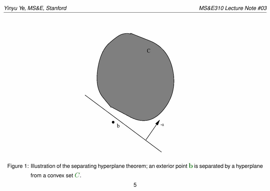
Figure 1: Illustration of the separating hyperplane theorem; an exterior point b is separated by a hyperplane

from a convex set C .

5


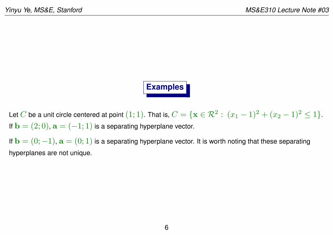
Examples

Let C be a unit circle centered at point (1; 1). That is, C = {x ∈ R2 : (x1 − 1)2 + (x2 − 1)2 ≤ 1}.

If b = (2; 0), a = (−1; 1) is a separating hyperplane vector.

If b = (0;−1), a = (0; 1) is a separating hyperplane vector. It is worth noting that these separating

hyperplanes are not unique.

6


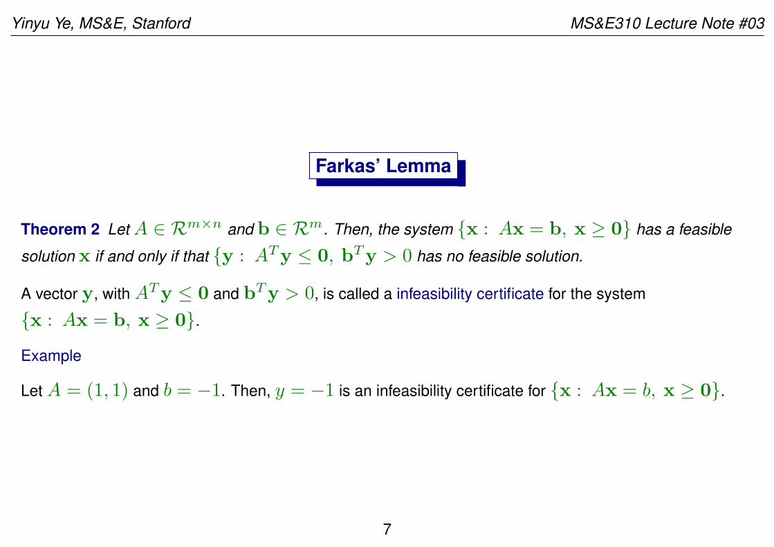
Farkas’ Lemma

Theorem 2 Let A ∈ Rm×n and b ∈ Rm. Then, the system {x : Ax = b, x ≥ 0} has a feasible

solution x if and only if that {y : ATy ≤ 0, bTy > 0 has no feasible solution.

A vector y, with ATy ≤ 0 and bTy > 0, is called a infeasibility certificate for the system

{x : Ax = b, x ≥ 0}.

Example

Let A = (1, 1) and b = −1. Then, y = −1 is an infeasibility certificate for {x : Ax = b, x ≥ 0}.

7


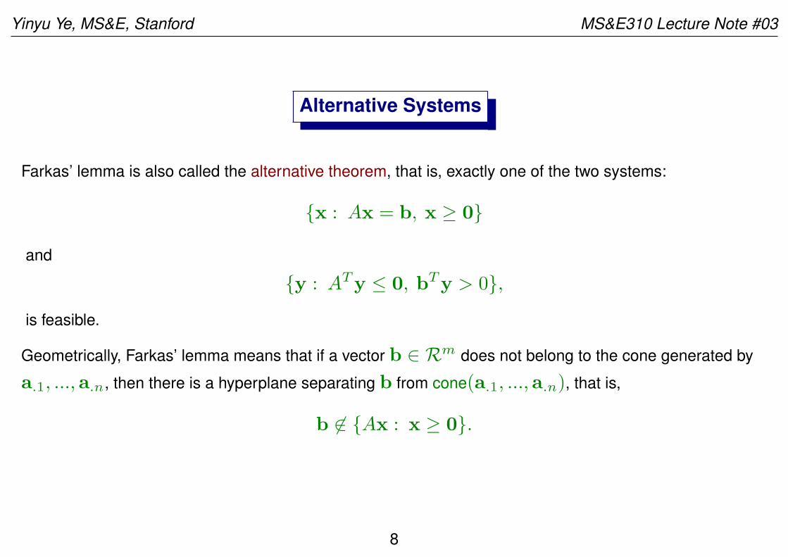
Alternative Systems

Farkas’ lemma is also called the alternative theorem, that is, exactly one of the two systems:

{x : Ax = b, x ≥ 0}

and

{y : ATy ≤ 0, bTy > 0},

is feasible.

Geometrically, Farkas’ lemma means that if a vector b ∈ Rm does not belong to the cone generated by

a.1, ...,a.n, then there is a hyperplane separating b from cone(a.1, ...,a.n), that is,

b ∈ {Ax : x ≥ 0}.

8


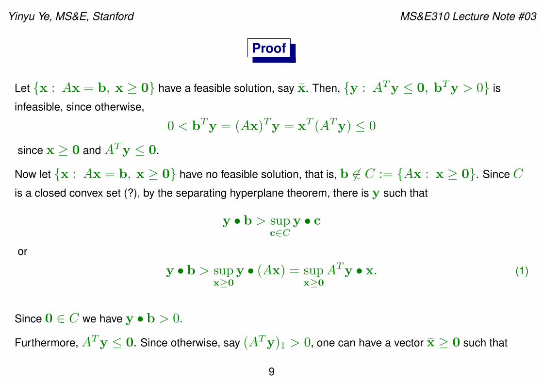
Proof

Let {x : Ax = b, x ≥ 0} have a feasible solution, say x. Then, {y : ATy ≤ 0, bTy > 0} is

infeasible, since otherwise,

0 < bTy = (Ax)Ty = xT (ATy) ≤ 0

since x ≥ 0 and ATy ≤ 0.

Now let {x : Ax = b, x ≥ 0} have no feasible solution, that is, b ∈ C := {Ax : x ≥ 0}. Since C

is a closed convex set (?), by the separating hyperplane theorem, there is y such that

y • b > supc∈C

y • c

or

y • b > supx≥0

y • (Ax) = supx≥0

ATy • x. (1)

Since 0 ∈ C we have y • b > 0.

Furthermore, ATy ≤ 0. Since otherwise, say (ATy)1 > 0, one can have a vector x ≥ 0 such that

9


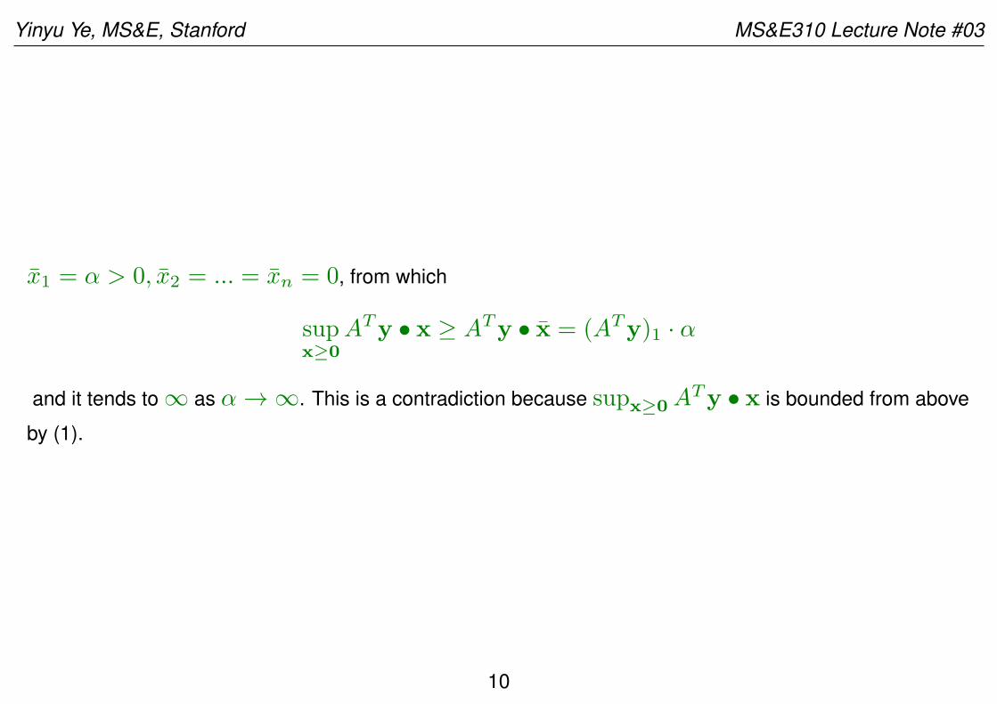
x1 = α > 0, x2 = ... = xn = 0, from which

supx≥0

ATy • x ≥ ATy • x = (ATy)1 · α

and it tends to ∞ as α → ∞. This is a contradiction because supx≥0 ATy • x is bounded from above

by (1).

10


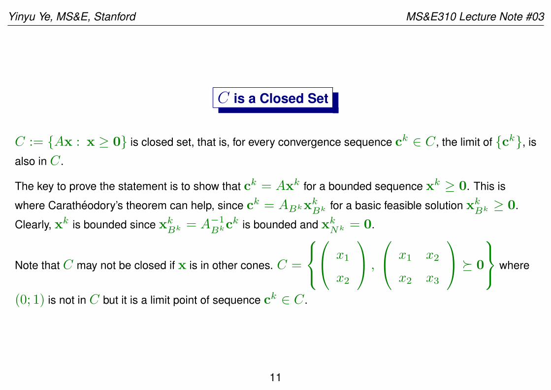
C is a Closed Set

C := {Ax : x ≥ 0} is closed set, that is, for every convergence sequence ck ∈ C , the limit of {ck}, is

also in C .

The key to prove the statement is to show that ck = Axk for a bounded sequence xk ≥ 0. This is

where Caratheodory’s theorem can help, since ck = ABkxkBk for a basic feasible solution xk

Bk ≥ 0.

Clearly, xk is bounded since xkBk = A−1

Bkck is bounded and xk

Nk = 0.

Note that C may not be closed if x is in other cones. C =

x1

x2

,

x1 x2

x2 x3

≽ 0

where

(0; 1) is not in C but it is a limit point of sequence ck ∈ C .

11


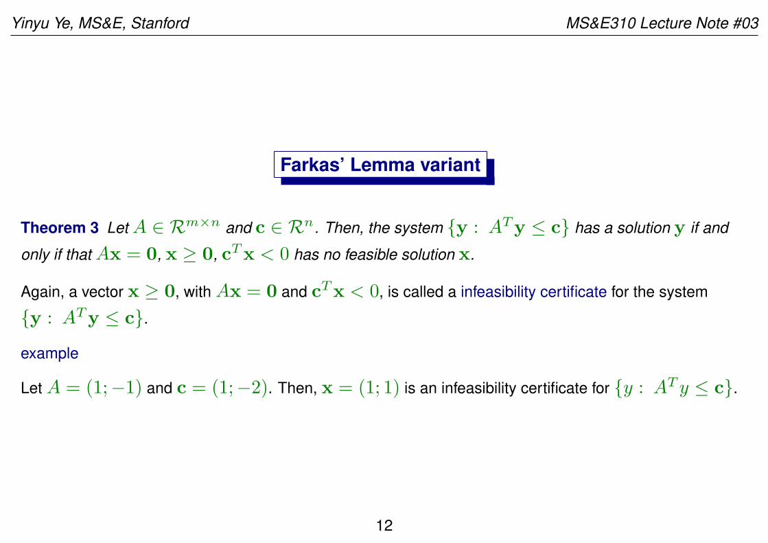
Farkas’ Lemma variant

Theorem 3 Let A ∈ Rm×n and c ∈ Rn. Then, the system {y : ATy ≤ c} has a solution y if and

only if that Ax = 0, x ≥ 0, cTx < 0 has no feasible solution x.

Again, a vector x ≥ 0, with Ax = 0 and cTx < 0, is called a infeasibility certificate for the system

{y : ATy ≤ c}.

example

Let A = (1;−1) and c = (1;−2). Then, x = (1; 1) is an infeasibility certificate for {y : AT y ≤ c}.

12


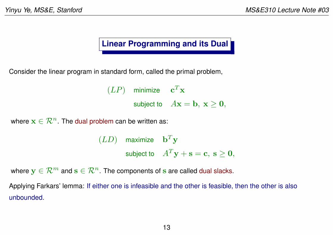
Linear Programming and its Dual

Consider the linear program in standard form, called the primal problem,

(LP ) minimize cTx

subject to Ax = b, x ≥ 0,

where x ∈ Rn. The dual problem can be written as:

(LD) maximize bTy

subject to ATy + s = c, s ≥ 0,

where y ∈ Rm and s ∈ Rn. The components of s are called dual slacks.

Applying Farkars’ lemma: If either one is infeasible and the other is feasible, then the other is also

unbounded.

13


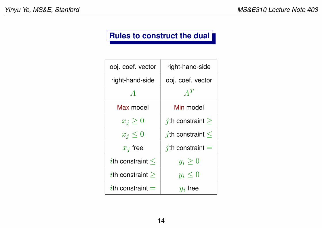
Rules to construct the dual

obj. coef. vector right-hand-side

right-hand-side obj. coef. vector

A AT

Max model Min model

xj ≥ 0 jth constraint ≥xj ≤ 0 jth constraint ≤xj free jth constraint =

ith constraint ≤ yi ≥ 0

ith constraint ≥ yi ≤ 0

ith constraint = yi free

14


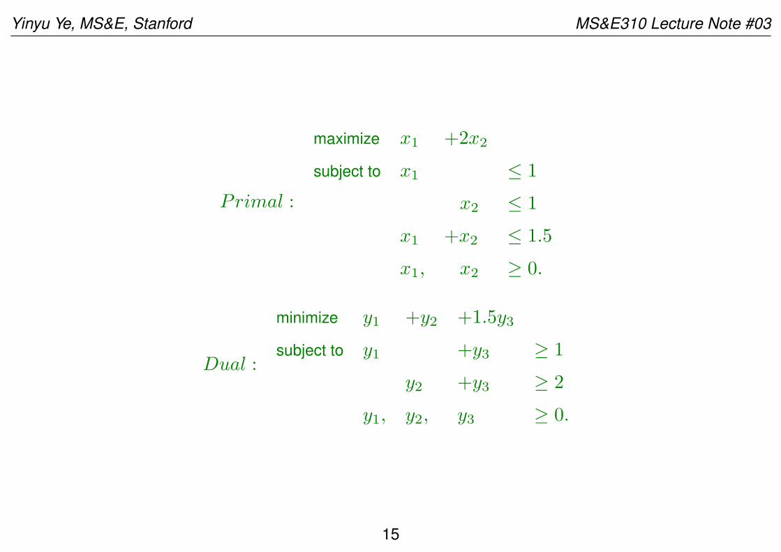
Primal :

maximize x1 +2x2

subject to x1 ≤ 1

x2 ≤ 1

x1 +x2 ≤ 1.5

x1, x2 ≥ 0.

Dual :

minimize y1 +y2 +1.5y3

subject to y1 +y3 ≥ 1

y2 +y3 ≥ 2

y1, y2, y3 ≥ 0.

15


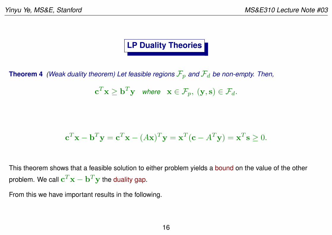
LP Duality Theories

Theorem 4 (Weak duality theorem) Let feasible regions Fp and Fd be non-empty. Then,

cTx ≥ bTy where x ∈ Fp, (y, s) ∈ Fd.

cTx− bTy = cTx− (Ax)Ty = xT (c−ATy) = xT s ≥ 0.

This theorem shows that a feasible solution to either problem yields a bound on the value of the other

problem. We call cTx− bTy the duality gap.

From this we have important results in the following.

16


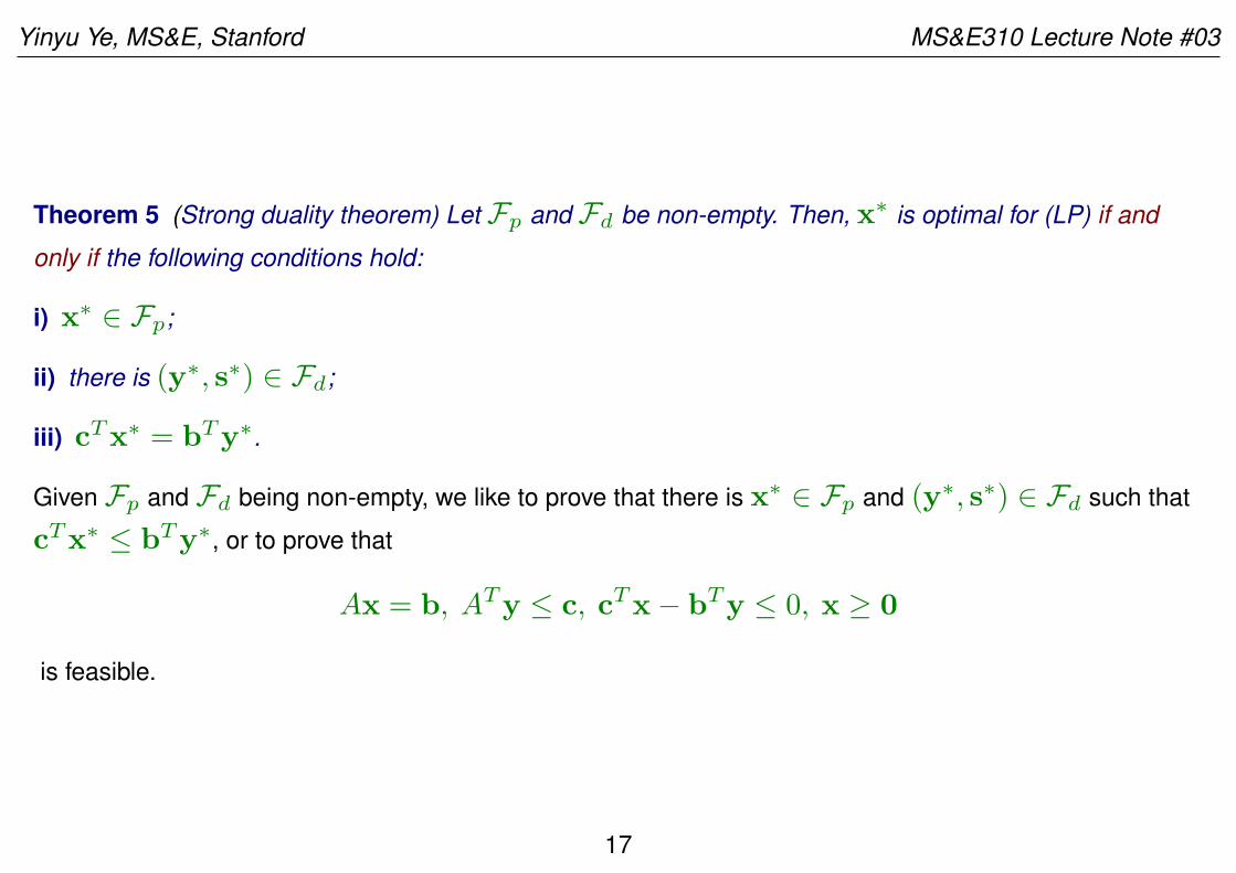
Theorem 5 (Strong duality theorem) Let Fp and Fd be non-empty. Then, x∗ is optimal for (LP) if and

only if the following conditions hold:

i) x∗ ∈ Fp;

ii) there is (y∗, s∗) ∈ Fd;

iii) cTx∗ = bTy∗.

Given Fp and Fd being non-empty, we like to prove that there is x∗ ∈ Fp and (y∗, s∗) ∈ Fd such that

cTx∗ ≤ bTy∗, or to prove that

Ax = b, ATy ≤ c, cTx− bTy ≤ 0, x ≥ 0

is feasible.

17


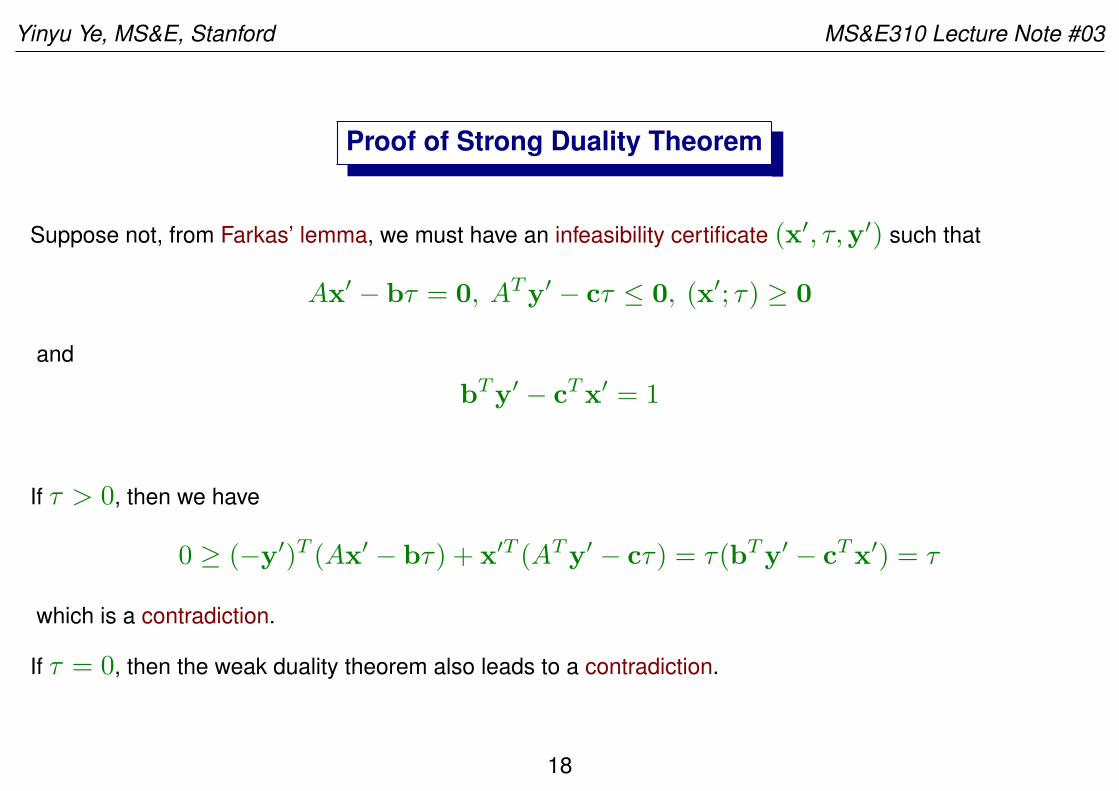
Proof of Strong Duality Theorem

Suppose not, from Farkas’ lemma, we must have an infeasibility certificate (x′, τ,y′) such that

Ax′ − bτ = 0, ATy′ − cτ ≤ 0, (x′; τ) ≥ 0

and

bTy′ − cTx′ = 1

If τ > 0, then we have

0 ≥ (−y′)T (Ax′ − bτ) + x′T (ATy′ − cτ) = τ(bTy′ − cTx′) = τ

which is a contradiction.

If τ = 0, then the weak duality theorem also leads to a contradiction.

18


Theorem 6 (LP duality theorem) If (LP) and (LD) both have feasible solutions then both problems have

optimal solutions and the optimal objective values of the objective functions are equal.

If one of (LP) or (LD) has no feasible solution, then the other is either unbounded or has no feasible

solution. If one of (LP) or (LD) is unbounded then the other has no feasible solution.

The above theorems show that if a pair of feasible solutions can be found to the primal and dual problems

with equal objective values, then these are both optimal. The converse is also true; there is no “gap.”

19


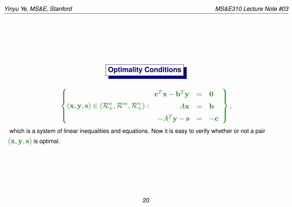
Optimality Conditions

(x,y, s) ∈ (Rn+,Rm,Rn

+) :

cTx− bTy = 0

Ax = b

−ATy − s = −c

,

which is a system of linear inequalities and equations. Now it is easy to verify whether or not a pair

(x,y, s) is optimal.

20


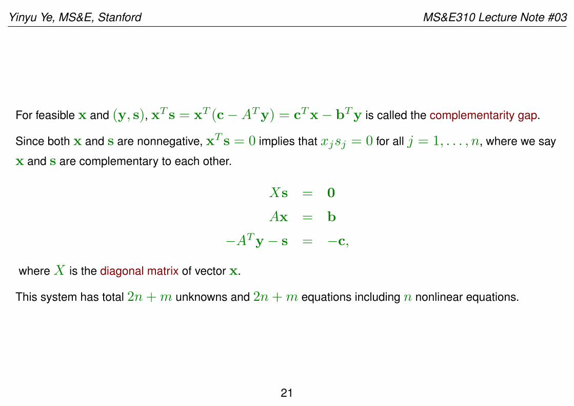
For feasible x and (y, s), xT s = xT (c−ATy) = cTx− bTy is called the complementarity gap.

Since both x and s are nonnegative, xT s = 0 implies that xjsj = 0 for all j = 1, . . . , n, where we say

x and s are complementary to each other.

Xs = 0

Ax = b

−ATy − s = −c,

where X is the diagonal matrix of vector x.

This system has total 2n+m unknowns and 2n+m equations including n nonlinear equations.

21


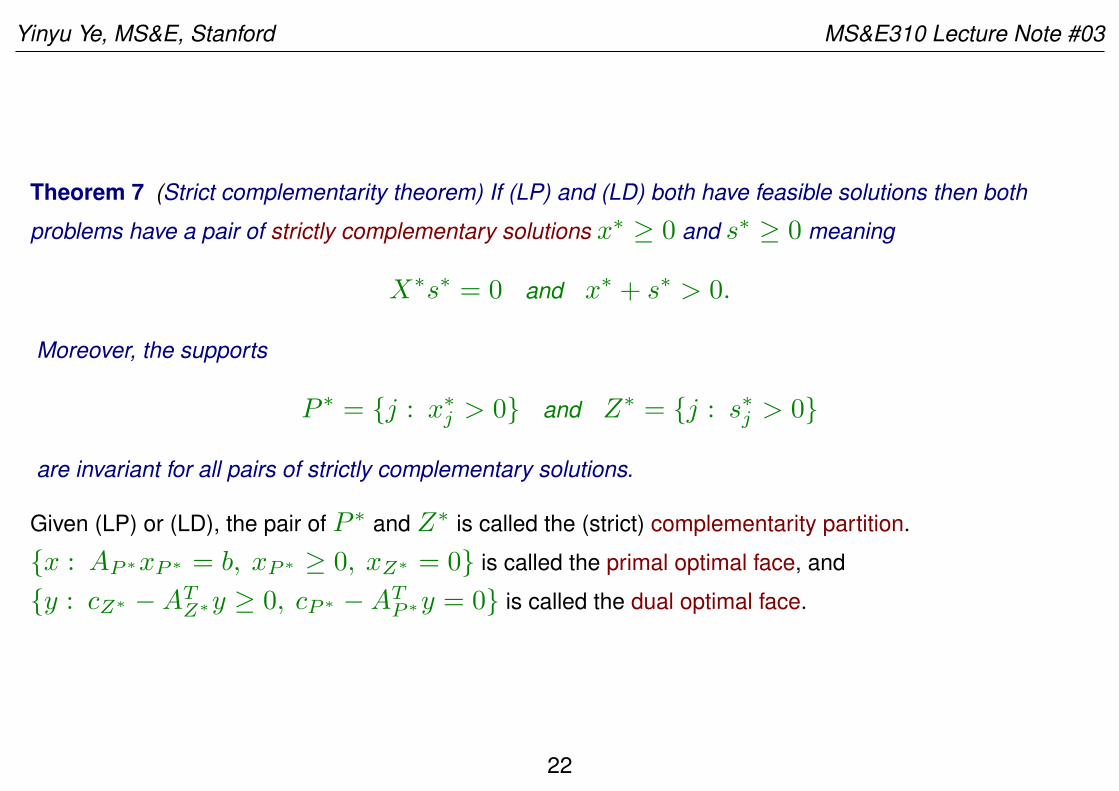
Theorem 7 (Strict complementarity theorem) If (LP) and (LD) both have feasible solutions then both

problems have a pair of strictly complementary solutions x∗ ≥ 0 and s∗ ≥ 0 meaning

X∗s∗ = 0 and x∗ + s∗ > 0.

Moreover, the supports

P ∗ = {j : x∗j > 0} and Z∗ = {j : s∗j > 0}

are invariant for all pairs of strictly complementary solutions.

Given (LP) or (LD), the pair of P ∗ and Z∗ is called the (strict) complementarity partition.

{x : AP∗xP∗ = b, xP∗ ≥ 0, xZ∗ = 0} is called the primal optimal face, and

{y : cZ∗ −ATZ∗y ≥ 0, cP∗ −AT

P∗y = 0} is called the dual optimal face.

22


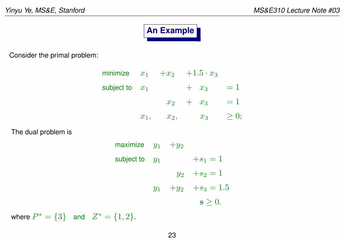
An Example

Consider the primal problem:

minimize x1 +x2 +1.5 · x3

subject to x1 + x3 = 1

x2 + x3 = 1

x1, x2, x3 ≥ 0;

The dual problem is

maximize y1 +y2

subject to y1 +s1 = 1

y2 +s2 = 1

y1 +y2 +s3 = 1.5

s ≥ 0.

where P ∗ = {3} and Z∗ = {1, 2}.

23


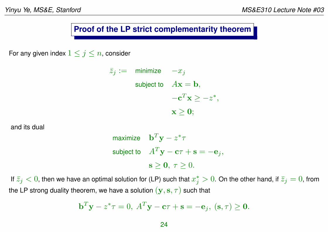
Proof of the LP strict complementarity theorem

For any given index 1 ≤ j ≤ n, consider

zj := minimize −xj

subject to Ax = b,

−cTx ≥ −z∗,

x ≥ 0;

and its dual

maximize bTy − z∗τ

subject to ATy − cτ + s = −ej ,

s ≥ 0, τ ≥ 0.

If zj < 0, then we have an optimal solution for (LP) such that x∗j > 0. On the other hand, if zj = 0, from

the LP strong duality theorem, we have a solution (y, s, τ) such that

bTy − z∗τ = 0, ATy − cτ + s = −ej , (s, τ) ≥ 0.

24


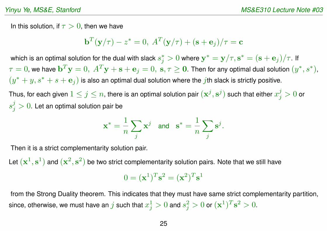
In this solution, if τ > 0, then we have

bT (y/τ)− z∗ = 0, AT (y/τ) + (s+ ej)/τ = c

which is an optimal solution for the dual with slack s∗j > 0 where y∗ = y/τ, s∗ = (s+ ej)/τ . If

τ = 0, we have bTy = 0, ATy + s+ ej = 0, s, τ ≥ 0. Then for any optimal dual solution (y∗, s∗),

(y∗ + y, s∗ + s+ ej) is also an optimal dual solution where the jth slack is strictly positive.

Thus, for each given 1 ≤ j ≤ n, there is an optimal solution pair (xj , sj) such that either xjj > 0 or

sjj > 0. Let an optimal solution pair be

x∗ =1

n

∑j

xj and s∗ =1

n

∑j

sj .

Then it is a strict complementarity solution pair.

Let (x1, s1) and (x2, s2) be two strict complementarity solution pairs. Note that we still have

0 = (x1)T s2 = (x2)T s1

from the Strong Duality theorem. This indicates that they must have same strict complementarity partition,

since, otherwise, we must have an j such that x1j > 0 and s2j > 0 or (x1)T s2 > 0.

25

Theory of Polyhedron and Duality - Stanford...

Documents

Transcript of Theory of Polyhedron and Duality - Stanford...