THEORY OF DISPERSED FIXED-DELAY INTERFEROMETRY … · The Astrophysical Journal Supplement Series,...
25
The Astrophysical Journal Supplement Series, 189:156–180, 2010 July doi:10.1088/0067-0049/189/1/156 C 2010. The American Astronomical Society. All rights reserved. Printed in the U.S.A. THEORY OFDISPERSED FIXED-DELAY INTERFEROMETRY FOR RADIAL VELOCITY EXOPLANET SEARCHES Julian C. van Eyken 1 ,2,5 , Jian Ge 1 ,5 , and Suvrath Mahadevan 1 ,3 ,4 ,5 1 Department of Astronomy, University of Florida, 211 Bryant Space Science Center, P.O. Box 112055, Gainesville, FL 32611-2055, USA; [email protected], [email protected]fl.edu, [email protected] 2 NASA Exoplanet Science Institute, California Institute of Technology, 770 South Wilson Avenue, M/S 100-22, Pasadena, CA 91125, USA 3 Department of Astronomy & Astrophysics, The Pennsylvania State University, University Park, PA 16802, USA 4 Center for Exoplanets and Habitable Worlds, The Pennsylvania State University, University Park, PA 16802, USA Received 2009 July 3; accepted 2010 May 28; published 2010 June 28 ABSTRACT The dispersed fixed-delay interferometer (DFDI) represents a new instrument concept for high-precision radial velocity (RV) surveys for extrasolar planets. A combination of a Michelson interferometer and a medium-resolution spectrograph, it has the potential for performing multi-object surveys, where most previous RV techniques have been limited to observing only one target at a time. Because of the large sample of extrasolar planets needed to better understand planetary formation, evolution, and prevalence, this new technique represents a logical next step in instrumentation for RV extrasolar planet searches, and has been proven with the single- object Exoplanet Tracker (ET) at Kitt Peak National Observatory, and the multi-object W. M. Keck/MARVELS Exoplanet Tracker at Apache Point Observatory. The development of the ET instruments has necessitated fleshing out a detailed understanding of the physical principles of the DFDI technique. Here we summarize the fundamental theoretical material needed to understand the technique and provide an overview of the physics underlying the instrument’s working. We also derive some useful analytical formulae that can be used to estimate the level of various sources of error generic to the technique, such as photon shot noise when using a fiducial reference spectrum, contamination by secondary spectra (e.g., crowded sources, spectroscopic binaries, or moonlight contamination), residual interferometer comb, and reference cross-talk error. Following this, we show that the use of a traditional gas absorption fiducial reference with a DFDI can incur significant systematic errors that must be taken into account at the precision levels required to detect extrasolar planets. Key words: instrumentation: interferometers – instrumentation: spectrographs – methods: analytical – planetary systems – techniques: radial velocities Online-only material: color figures 1. THE DFDI CONCEPT AND THE ET PROGRAM 1.1. The Need for a New Instrument Despite the remarkable achievements in extrasolar planet detection over the last decade, identification of many more planets is still needed to constrain formation and evolutionary models. This is partially because of the unexpected diversity of planet properties uncovered, and partially because of a lack of large, well-defined, unbiased target search lists—the primary concern naturally having been to find planets in the first place. To this point many surveys have been subject to completeness issues or in some cases deliberate biases toward planet detection (e.g., da Silva et al. 2006), making it difficult to perform robust statistical analyses of the known planet sample. Armitage (2007) concluded that there is still a strong need for large uniform surveys to enlarge the statistical sample available: drawing on the unbiased survey of Fischer & Valenti (2005), he was only able to find a uniform subsample of 22 of the over 170 planets then known that satisfied the requirements for a statistical comparison with models. A few thousand stars have been searched between the various RV surveys since the first RV discoveries of giant extrasolar 5 Visiting Astronomers, Kitt Peak National Observatory, National Optical Astronomy Observatory, which is operated by the Association of Universities for Research in Astronomy, Inc. (AURA), under cooperative agreement with the National Science Foundation. planets around solar-type stars (Mayor & Queloz 1995), includ- ing a large fraction of the late-type, stable stars down to visual magnitude ∼8. Improved instrument light throughput would help facilitate the survey of fainter stars. (A review of radial ve- locity (RV) discoveries is given by Udry et al. 2007.) Although the rate of detections from transit surveys will likely increase, transit surveys can only detect the small fraction of planets which happen to eclipse their parent stars (∼10% probability for hot Jupiters, from geometrical considerations— Kane et al. 2004). Furthermore, the complementary information gained from RV detections remains of great value. There is therefore a strong case for finding a technique capable of RV surveys down to faint magnitudes and at faster speeds than have been achieved over the last decade. The Exoplanet Tracker (ET) instruments are a new type of fiber-fed RV instrument based on the “dis- persed fixed-delay interferometer” (DFDI), built with the goal of satisfying this requirement. 1.2. The DFDI Principle The RV technique for detecting exoplanets consists in mea- suring the reflex motion of the parent star due to an orbiting planet by measuring very precisely the resulting Doppler shifts of the stellar absorption lines. Achieving this requires extremely high precision: internal precisions now typically reach down to the 3 m s −1 level (Butler et al. 1996; Vogt et al. 2000), and even as low as 1 m s −1 or better (Pepe et al. 2005). For com- parison, a Jupiter analog in a circular orbit around a solar-type 156
Transcript of THEORY OF DISPERSED FIXED-DELAY INTERFEROMETRY … · The Astrophysical Journal Supplement Series,...
The Astrophysical Journal Supplement Series, 189:156–180, 2010 July doi:10.1088/0067-0049/189/1/156C© 2010. The American Astronomical Society. All rights reserved. Printed in the U.S.A.
THEORY OF DISPERSED FIXED-DELAY INTERFEROMETRY FOR RADIAL VELOCITYEXOPLANET SEARCHES
Julian C. van Eyken1,2,5
, Jian Ge1,5
, and Suvrath Mahadevan1,3,4,5
1 Department of Astronomy, University of Florida, 211 Bryant Space Science Center, P.O. Box 112055, Gainesville, FL 32611-2055, USA;[email protected], [email protected], [email protected]
2 NASA Exoplanet Science Institute, California Institute of Technology, 770 South Wilson Avenue, M/S 100-22, Pasadena, CA 91125, USA3 Department of Astronomy & Astrophysics, The Pennsylvania State University, University Park, PA 16802, USA
4 Center for Exoplanets and Habitable Worlds, The Pennsylvania State University, University Park, PA 16802, USAReceived 2009 July 3; accepted 2010 May 28; published 2010 June 28
ABSTRACT
The dispersed fixed-delay interferometer (DFDI) represents a new instrument concept for high-precision radialvelocity (RV) surveys for extrasolar planets. A combination of a Michelson interferometer and a medium-resolutionspectrograph, it has the potential for performing multi-object surveys, where most previous RV techniqueshave been limited to observing only one target at a time. Because of the large sample of extrasolar planetsneeded to better understand planetary formation, evolution, and prevalence, this new technique represents alogical next step in instrumentation for RV extrasolar planet searches, and has been proven with the single-object Exoplanet Tracker (ET) at Kitt Peak National Observatory, and the multi-object W. M. Keck/MARVELSExoplanet Tracker at Apache Point Observatory. The development of the ET instruments has necessitatedfleshing out a detailed understanding of the physical principles of the DFDI technique. Here we summarizethe fundamental theoretical material needed to understand the technique and provide an overview of thephysics underlying the instrument’s working. We also derive some useful analytical formulae that can be usedto estimate the level of various sources of error generic to the technique, such as photon shot noise whenusing a fiducial reference spectrum, contamination by secondary spectra (e.g., crowded sources, spectroscopicbinaries, or moonlight contamination), residual interferometer comb, and reference cross-talk error. Followingthis, we show that the use of a traditional gas absorption fiducial reference with a DFDI can incur significantsystematic errors that must be taken into account at the precision levels required to detect extrasolar planets.
Key words: instrumentation: interferometers – instrumentation: spectrographs – methods: analytical – planetarysystems – techniques: radial velocities
Online-only material: color figures
1. THE DFDI CONCEPT AND THE ET PROGRAM
1.1. The Need for a New Instrument
Despite the remarkable achievements in extrasolar planetdetection over the last decade, identification of many moreplanets is still needed to constrain formation and evolutionarymodels. This is partially because of the unexpected diversityof planet properties uncovered, and partially because of a lackof large, well-defined, unbiased target search lists—the primaryconcern naturally having been to find planets in the first place.To this point many surveys have been subject to completenessissues or in some cases deliberate biases toward planet detection(e.g., da Silva et al. 2006), making it difficult to perform robuststatistical analyses of the known planet sample. Armitage (2007)concluded that there is still a strong need for large uniformsurveys to enlarge the statistical sample available: drawing onthe unbiased survey of Fischer & Valenti (2005), he was onlyable to find a uniform subsample of 22 of the over 170 planetsthen known that satisfied the requirements for a statisticalcomparison with models.
A few thousand stars have been searched between the variousRV surveys since the first RV discoveries of giant extrasolar
5 Visiting Astronomers, Kitt Peak National Observatory, National OpticalAstronomy Observatory, which is operated by the Association of Universitiesfor Research in Astronomy, Inc. (AURA), under cooperative agreement withthe National Science Foundation.
planets around solar-type stars (Mayor & Queloz 1995), includ-ing a large fraction of the late-type, stable stars down to visualmagnitude ∼8. Improved instrument light throughput wouldhelp facilitate the survey of fainter stars. (A review of radial ve-locity (RV) discoveries is given by Udry et al. 2007.) Althoughthe rate of detections from transit surveys will likely increase,transit surveys can only detect the small fraction of planets whichhappen to eclipse their parent stars (∼10% probability for hotJupiters, from geometrical considerations— Kane et al. 2004).Furthermore, the complementary information gained from RVdetections remains of great value. There is therefore a strongcase for finding a technique capable of RV surveys down tofaint magnitudes and at faster speeds than have been achievedover the last decade. The Exoplanet Tracker (ET) instrumentsare a new type of fiber-fed RV instrument based on the “dis-persed fixed-delay interferometer” (DFDI), built with the goalof satisfying this requirement.
1.2. The DFDI Principle
The RV technique for detecting exoplanets consists in mea-suring the reflex motion of the parent star due to an orbitingplanet by measuring very precisely the resulting Doppler shiftsof the stellar absorption lines. Achieving this requires extremelyhigh precision: internal precisions now typically reach down tothe 3 m s−1 level (Butler et al. 1996; Vogt et al. 2000), andeven as low as 1 m s−1 or better (Pepe et al. 2005). For com-parison, a Jupiter analog in a circular orbit around a solar-type
156
No. 1, 2010 THEORY OF DFDI FOR RADIAL VELOCITY EXOPLANET SEARCHES 157
star would cause sinusoidal RV variations with an amplitude ofabout 12.5 m s−1. Exoplanet RV surveys have traditionally de-pended on recording very high resolution echelle spectra, eithercross-correlating the spectra with reference template spectra, orfitting functions to the line profiles themselves to measure thepositions of the centroids.
The DFDI technique, upon which the ET instruments arebased, comprises a Michelson interferometer followed by alow- or medium-resolution post-disperser (also referred to byErskine 2003 as an externally dispersed interferometer, or“EDI,” emphasizing the distinction from techniques wherethe dispersing element is internal to the interferometer). Theeffective resolution of the instrument is primarily determinedby the interferometer, so the post-dispersing spectrograph canbe of much lower resolution than in traditional dispersivetechniques, and consequently can be smaller, cheaper, and havehigher throughput (Ge 2002; Ge et al. 2003a, 2003b). Thetechnique is closely related to Fourier transform spectroscopy:the post-disperser effectively creates a continuum of very narrowbandpasses for the interferometer, increasing the interferencefringe contrast. All of the information needed is contained inthe fringe phase and visibility. It emerges that since we are onlyinterested in the Doppler shift of the lines, measurements arerequired at essentially only one value of interferometer delay(hence “fixed delay”).
The cost of the instrument is comparatively low, and mostimportantly, it can operate in a single-order mode: wheretraditional echelle spectrograph techniques operate by spreadinga single stellar spectrum over an entire CCD detector in multipleorders, here the spectrum only takes up one strip along thedetector. Spectra from multiple stars can therefore be lined up atonce on a single detector. In combination with a wide-field multi-fiber telescope, this makes multi-object RV planet surveyingpossible (Ge 2002; Ge et al. 2002; Mahadevan et al. 2003). Themulti-object Keck ET instrument based on the DFDI techniqueis one of the first instruments to be built with this purpose (Geet al. 2009).6
The very high levels of precision required for planet detectionand the difficulty of directly measuring absolute wavelengthsmean that some kind of stationary reference spectrum is invari-ably used as a calibration. Various types of fiducial referencehave been employed to overcome these problems (e.g., Griffin& Griffin 1973; Campbell & Walker 1979), but the references ofchoice have generally become ThAr emission lamps (Baranneet al. 1996) and iodine vapor absorption cells placed withinthe optical beam path (Butler et al. 1996). In this respect, theET instruments are the same, and we discuss the use of suchreferences with the DFDI technique in this paper.
1.3. A Brief History
The idea of using the combination of a Michelson interfer-ometer with a post-disperser was first proposed for precisionDoppler planet searches by D. J. Erskine in 1997, at LawrenceLivermore National Laboratory (Erskine & Ge 2000; Ge 2002;Ge et al. 2002; Erskine 2003). The same approach is beingfollowed by Edelstein et al. (2006) in the infrared, in an at-tempt to find planets around late-type stars. A similar approachis discussed by Mosser et al. (2003) for asteroseismology andthe measurement of stellar oscillations; more recently the tech-
6 Comparable traditional dispersive multi-object instruments are the VLTGIRAFFE and UVES/FLAMES spectrographs (Loeillet et al. 2008), and theMMT Hectochelle (Szentgyorgyi & Furesz 2007).
nique has also been adopted for the USNO Dispersed FourierTransform Spectrograph (dFTS) instrument (Hajian et al. 2007;Behr et al. 2009; in this last case, the interferometer delay isalso varied so that high-resolution spectra can be reconstructedin addition to extracting Doppler shift information—see alsoErskine & Edelstein 2004).
The idea of dispersed interferometry itself is by no meansnew: Michelson himself recognized the use of interferometersfor spectroscopy (Michelson 1903), and even proposed combin-ing a disperser in series with a Michelson interferometer. In thiscase the disperser, a prism, was placed before the interferometer,allowing only a narrow bandwidth of light to enter the interfer-ometer in the first place. In what was likely the first realizationof a DFDI, Edser & Butler (1898) placed a Fabry–Perot typeinterferometer in front of a spectrograph7 to produce dispersedfringes (effectively an interferometer comb—see Section 2.4),which they used as a fiducial reference for measuring the wave-lengths of spectral lines. Such dispersed fringes were later tobecome known as “Edser–Butler fringes” (Lawson 2000).
Somewhat later, along with the development of P. Connes’spectrometre interferentiel a selection par l’amplitude de modu-lation (SISAM; described in Jacquinot 1960), various combina-tions of interferometers with dispersers began to be seen in thefield of astronomy. Examples include Geake et al. (1959), usinga Fabry–Perot in front of a spectrograph to increase throughput;and the later spatial heterodyne spectroscopy (SHS; Harlanderet al. 1992) and heterodyned holographic spectroscopy (HHS;Frandsen et al. 1993; Douglas 1997) techniques, using inter-nally dispersed interferometers, where the interferometer mir-rors were replaced with gratings. Barker & Hollenbach (1972)outlined an early example of the use of true fixed-delay inter-ferometry for velocimetry, measuring the velocities of laser-illuminated projectiles in the laboratory. The use of a Michel-son interferometer for actual astronomical RV measurementswas proposed shortly afterward by Gorskii & Lebedev (1977)and Beckers & Brown (1978). Forrest & Ring (1978) also pro-posed using a Michelson interferometer with a fixed delay forhigh-precision Doppler measurements of single spectral linesfor the detection of stellar oscillations, and more recent exam-ples of similar spectroscopic techniques include Connes (1985)and McMillan et al. (1993, 1994). Others have also used sim-ilar techniques for Doppler imaging over very narrow band-passes, notably the wide-angle Doppler imaging interferometer(WAMDII) and Global Oscillation Network Group (GONG)projects (Shepherd et al. 1985; Harvey & The GONG Instru-ment Team 1995).
Many of these interferometric instruments, however, sufferedfrom the limitation of having an extremely narrow bandpass,tending to limit their application to only bright targets. TheDFDI technique used in the ET instruments allows for an ar-bitrarily wide bandpass, limited only by the spectrograph ca-pabilities, while still retaining the high-resolution spectral in-formation needed for precision velocity measurements. Thefirst such DFDI instruments were built at the Lawrence Liver-more National Laboratory and the Lick 1 m telescope between1997 and 1999, and were reported in Erskine & Ge (2000)and Ge et al. (2002). The ET project was undertaken shortlyafter.
7 It was mistakenly stated in van Eyken et al. (2004a) that Edser & Butler(1898) used a Michelson rather than a Fabry–Perot interferometer, which hascertain disadvantages in this application (D. J. Erskine 2005, privatecommunication).

158 VAN EYKEN, GE, & MAHADEVAN Vol. 189
1.4. The ET Project
The ET project began at Penn State University in 2000,continuing at the University of Florida from 2004. Early labtests were performed at Penn State, and prototype test runswere conducted at the McDonald Observatory Hobby-EberlyTelescope in late 2001, and at the Palomar 200 inch telescopein early 2002 (Ge et al. 2003b; Mahadevan 2006).
Two ET instruments have now been built: the single-objectprototype ET (van Eyken et al. 2004b; Mahadevan et al. 2008a),permanently installed at the KPNO 2.1 m telescope in 2003after a temporary test run in 2002 August; and the multi-objectKeck ET, first installed at the APO Sloan 2.5 m telescope in 2005March, upgraded and moved to a more stable location at the sametelescope later that year, and then further upgraded and fullyinstalled as facility instrument housed in its own custom-builtroom in 2008 September. The latter instrument will functionas the workhorse for the SDSS-III “Multi-object APO RadialVelocity Exoplanet Large-area Survey” (MARVELS; Ge et al.2009).
Proof of concept was achieved using the KPNO ET withthe first DFDI planet detection, a confirmation of the knowncompanion to 51 Pegasi (van Eyken et al. 2004a). Our first planetdiscovery, HD 102195b (ET-1), was also later made using thisinstrument (Ge et al. 2006). The multi-object Keck ET is a fullscale instrument developed to satisfy the survey requirementslaid out in Section 1.1, and it is anticipated that it will be able tomake a significant contribution to the field of extrasolar planetsearches over the next decade (Ge et al. 2009).
2. INSTRUMENT PRINCIPLES AND THEORY
Although various forms of the DFDI have been employedbefore, the concept, particularly in its specific application toexoplanet finding, is rather new. Much of the work in under-standing the data from the instrument has therefore involvedcoming to a full understanding of the physics of the instrumentitself. Related theory is discussed in a number of sources (forexample, Goodman 1985; Erskine & Ge 2000; Lawson 2000;Ge 2002; Ge et al. 2002; Erskine 2003; Mosser et al. 2003;van Eyken et al. 2003); an attempt is made here to draw to-gether, expand on, and precisely state the theoretical materialneeded for a complete understanding of the instrument, and toprovide an overview of the physics underlying the instrument’sworking from the perspective of precision RV planet detection.The approach taken here allows for some important insights,particularly regarding certain errors arising from the use of acommon-path fiducial reference spectrum such as that from aniodine gas absorption cell. In addition, we derive in Section 3some useful general formulae that can be applied to estimateanalytically the magnitude of both these and a number of othertypes of error generic to the technique.
Taken together, this discussion should provide some ofthe fundamentals necessary for understanding and interpretingDFDI data. Appendix B gives a derivation showing the relationto the approach employed by Erskine (2003), to which theapproach here is complementary.
2.1. Formation of a Fringing Spectrum
Figure 1 shows a highly simplified schematic of a DFDI,consisting of the two main components, a fiber-fed Michelsoninterferometer and a disperser, followed by a detector. Lightinput from the fiber is split into two paths along the arms ofthe interferometer and then recombined at the beamsplitter. The
output is fed to the disperser, represented for convenience as aprism, though generally this will be a spectrograph. An etalonis placed in one of the interferometer arms to create a fixedoptical path difference (or “delay”), d = d0, between the twoarms, while allowing for adequate field widening (Hilliard &Shepherd 1966; Mahadevan et al. 2008a). d0 is typically on theorder of millimeters. In practice, an iodine vapor cell can alsobe placed in the optical path before or after the interferometerto act as a fiducial reference (Section 2.6).
Inputting a wide collimated beam of monochromatic lightinto the instrument with both interferometer mirrors exactlyperpendicular to the light travel path will give either a bright ora dark fringe at the output of the interferometer (Figure 1(A)),depending on whether the exact path difference d between thetwo arms corresponds to constructive or destructive interference.If we were to scan one of the mirrors back and forth, the flux atthe interferometer output would vary sinusoidally as a functionof d. If we now tilt this mirror along the axis in the plane of thepage, we effectively scan a small range of delays along they-direction (i.e., perpendicular to the axis of the tilt and inthe plane of the mirror, corresponding to the slit direction inthe spectrograph). Hence we would see a series of parallel brightand dark fringes, now varying sinusoidally as a function of y.8
Consider first a very high (actually infinite) resolution spec-trograph disperser for the sake of argument: following the beamthrough until it reaches the detector plane would result in a singleemission line with fringes along the slit direction, as shown inFigure 1(C). Switching the input spectrum to white light, whichcan be thought of as a continuum of neighboring delta functionsin wavelength (λ) space, leads to a similar fringe pattern on thedetector at every wavelength channel. Due to the fact that, interms of the number of wavelengths, the optical path differenceis different for different wavelengths, each fringe is slightly off-set in phase from its neighbors (and very slightly different inperiod). This gives rise to the series of parallel lines known asthe interferometer “comb,” shown in Figure 1(D). Going fur-ther and inputting a stellar spectrum into the instrument wouldsimply give the product of the stellar spectrum and the comb,as in Figure 1(E). Finally, changing to the real case of a low- ormedium-resolution spectrograph as for an ET-type instrument,the comb is no longer (or barely) resolved, and we see a spec-trum like that in Figure 1(F). Such a spectrum is sometimesreferred to as a spectrum “channeled with fringes,” also knownas Edser–Butler fringes (Edser & Butler 1898; Lawson 2000;Ge 2002). The remaining fringes contain high spatial frequencyDoppler information that has been heterodyned down to lowerspatial frequencies by the interferometer comb (Erskine 2003;Mahadevan 2006). It is this heterodyning that allows for the useof a low-resolution spectrograph at low dispersion, and is thekey to the DFDI technique.
2.2. Fringe Phase and Visibility
Above we outlined a simple intuitive way of understandingthe formation of the DFDI fringing spectrum. For a fullmathematical description, we proceed by a slightly differentroute. Each wavelength channel on the detector has an associatedsinusoidal fringe running along the slit direction, where by“channel,” we mean specifically an infinitesimally wide strip
8 Another way of sampling the fringes is to scan the interferometer delay invery small steps (see Erskine 2003): this allows for certain advantages incalibration as well as a one-dimensional spectrum which requires less detectorreal estate, but comes at the disadvantage of requiring an actively controlledinterferometer. The principles are the same, however.

No. 1, 2010 THEORY OF DFDI FOR RADIAL VELOCITY EXOPLANET SEARCHES 159
or
y
(mirror 2 untilted)
(mirror 2 tilted)
y
Mirror 2
Mirror 1
Detector
Disperser
y
λ
Etalon
A
B
{
Michelson interferometer
Input from fiber
C
F
Beamsplitter
E
D
Monochromatic
White light
Stellar spectrum
Stellar spectrum/low R
Figure 1. Dispersed interferometer schematic. y corresponds to position in the slit direction (directed out of the page in the interferometer schematic), and λ indicateswavelength in the dispersion direction. (A) Output from interferometer alone with monochromatic light input, and mirror 2 untilted. (B) The same with mirror 2 tiltedalong the axis in the plane of the page, as shown. (C) Image on detector with monochromatic light at very high resolution. One fringed emission line is seen. (D)Detector image with white light input. (E) Image with stellar spectrum input. (F) As for E but at low resolution.
(A color version of this figure is available in the online journal.)

160 VAN EYKEN, GE, & MAHADEVAN Vol. 189
of the spectrum along the slit direction at pixel position j, wherej need not necessarily be an integer. A given fringe has anassociated phase and visibility, where visibility is a measure ofthe contrast in the fringe, defined as the ratio of the amplitudeof the fringe to its central (mean) flux value. Equivalently, thiscan be stated as (Imax − Imin)/(Imax + Imin), where Imax andImin are the maximum and minimum flux values in the fringe(Michelson 1903). Here we introduce the concept of a “whirl”(Erskine & Ge 2000): the phase and visibility for a fringe cantogether be thought of as representing a vector, with the visibilityrepresenting the magnitude. These quantities can be determinedin a number of ways; in general we simply fit a sinusoid.An ensemble of such vectors representing a full spectrum ofchannels is called a whirl. The whirl is the directly measuredquantity from a fringing spectrum and contains the informationrelevant to velocity determination. Vector operations such asaddition, subtraction, and scalar products can be performed onthese whirls just as for the individual vectors (Erskine & Ge2000).
To understand what determines the values of the phase andvisibility for a fringe, we can consider the contribution fromeach wavelength of light to a particular channel on the detector(remembering that although the channel is infinitesimally widein its spacial extent in the dispersion direction, it still has afinite bandwidth). Each contributing wavelength has passedthrough the interferometer, and for an ideal interferometer, it willcontribute a sinusoid of 100% visibility like that in Figure 1(C).The flux of these sinusoids on the detector can each be describedby �{1 + exp(i2πd/λ)}, where d varies linearly with positiony along the length of the slit, and �{. . .} represents the realpart of a complex expression. Since the spectrograph has finiteresolution, a narrow band of such wavelengths will contribute toany given channel, owing to the overlap of line spread functions(LSFs) from neighboring wavelengths. The measured fringealong the slit direction is a continuous summation of thosesinusoids, weighted by the flux of the spectrum contributingto that channel, Qj (λ), where Q is given by the productof the power spectrum coming into the instrument and thespectrograph response function at that channel on the detector.We use the term “spectrograph response function” throughoutto refer to the light throughput as a function of wavelength ata given infinitesimal point on the detector, or equivalently, ata given channel in the image on the detector. (This is distinctfrom, though closely related to, the LSF—see Appendix A.)
Switching from wavelength to wavenumber κ ≡ 1/λ, anddropping the j subscript for simplicity, the summation ofsinusoids can be expressed as
I (d) =∫
Q(κ) �{1 + ei2πκd} dκ
=∫
Q(κ) dκ + �{∫
Q(κ)ei2πκd dκ
}, (1)
where I (d) is the measured flux along the slit direction. The firstterm on the right-hand side is simply the total integrated flux inthe channel, which must be real valued. The second term canimmediately be identified as the real part of a Fourier transform,�{F[Q]d}, with delay as the conjugate variable to wavenumber,and shows the close relationship between DFDI instruments andFourier transform spectroscopy (Jacquinot 1960).
Normalizing by dividing through by the total flux, we candefine the complex quantity α such that
Inorm(d) = 1 + �{F[Q(κ)]d∫
Q(κ) dκ
}= 1 + �{α}, (2)
where
α ≡ αeiφα ≡ F[Q(κ)]d∫Q(κ) dκ
. (3)
This is the fundamental equation for DFDI fringe formation:the quantity α is the “complex degree of coherence” (Goodman1985), and describes the phase, φα , and amplitude, α, of thenormalized fringes (i.e., the visibility), as a function of d and theinput spectrum. α is referred to here as the complex visibility.9
More rigorous derivations of this can be found in Goodman(1985, chap. 5) and Lawson (2000), but this explanation isadequate for our purposes.
In order to understand the actual form of the fringes seen ina DFDI, it is important to realize that the portion of spectrumcontributing to any given channel, Q, has a very narrow passband(for the ET instruments, Δλ/λ ∼ 1 Å/5000 Å = 2 × 10⁻⁴).We imagine Q as being a shifted version of a function Q0,where Q0 has a characteristic width Δκ and is centered at zerowavenumber. We shift Q0 in wavenumber so that its center fallsat wavenumber κ = κ , and we have Q(κ) = Q0(κ − κ). By theFourier shift theorem we can write
F[Q]d = F[Q0(κ − κ)]d = e−i2πdκF[Q0]d . (4)
The right-hand side shows two components. The exponentialterm represents a linear phase variation with delay, varyingon the scale of the period 1/κ . The second term, the Fouriertransform, represents a modulation of this signal. By thereciprocal scaling property of Fourier transforms, the secondterm can be expected to vary on minimum length scales of theorder of the reciprocal of the width of Q0, that is, on scales of1/Δκ . Since 1/Δκ � 1/κ , Equation (4) represents a sinusoidalfringe of frequency κ modulated by a slow variation in bothphase and amplitude. To see this more clearly, we can substituteEquation (4) into the first expression on the right-hand side ofEquation (2) and write
Inorm(d) = 1 +�{e−i2πdκF[Q0]d}∫
Q(κ) dκ. (5)
If we define
α0(d) ≡ α0(d)eiφα0 (d) ≡ F[Q0]d∫Q(κ) dκ
, (6)
we can rewrite Equation (5) as
Inorm(d) = 1 + �{α0(d)e−i2πdκ}= 1 + α0(d) cos(2πdκ − φα0 (d)) (7)
(where we have simplified the negative in the cosine term usingthe symmetry of the cosine function). This clearly shows theform of the fringe. Over large ranges of d, the fringe appearslike a “carrier wave,” given by the cosine term, that is slowlymodulated in phase and amplitude by an envelope α0 (the“coherence envelope,” Lawson 2000). Over the length of the
9 The quantity is generally represented by the letter γ in the literature cited.We use α here instead purely for clearer distinction between bold-faced vectorand regular-faced amplitude representations.

No. 1, 2010 THEORY OF DFDI FOR RADIAL VELOCITY EXOPLANET SEARCHES 161
norm
1/Δκ 3/Δκ2/Δκ 0d
Δ d
||α0α
Sinusoidal term
d
I
Envelope,
Figure 2. Interferogram showing the coherence envelope due to a rectangular bandpass modulating the sinusoidal fringe. Along the slit direction of a fringing spectrum,a very small part of the interferogram is sampled over the range d0 ± Δd/2.
slit direction on the detector, we sample only a very small rangeof delays, d0 −Δd/2 � d � d0 +Δd/2, where d0 is determinedby the interferometer etalon, as before, and Δd is typically afew wavelengths. Over this range, the variation in α0 is smallas we show below, so we see only an approximately uniformsinusoid (see Figure 2) along a single wavelength channel on thedetector. In measuring the phase and visibility of this fringe, weessentially make a measurement of α0 at the fixed delay d = d0.The phase offset of the sinusoid is determined by the argumentof α0, φα0 . The measured (absolute) fringe visibility is simplythe amplitude of the normalized fringe, α0.
In general, we can estimate a rough order of magnitude forthe fractional change in the magnitude of the visibility betweenconsecutive sinusoid peaks by comparing the variation lengthscales: to order of magnitude, we can expect α0 to vary byof order α0 on scales of 1/Δκ , so that over one period ofthe sinusoid, 1/κ , it will vary by Δα0 = α0Δκ/κ = α0/R,where R is the spectrograph resolution. Since for any inputspectrum, 1/Δκ determines the fastest variation scale for theenvelope, this represents an upper limit. For the ET instruments,R ∼ 5000, so that over the length of the slit (a few fringes)Δα0/α0 ∼ 10−3. In practice, such a small variation will usuallybe significantly below the measurement errors in fringe phaseand visibility due to photon noise for even the brightest sources,and would correspond to a final velocity error of ∼0.1 m s−1 foran instrument similar to the KPNO ET.10 Even in the event thatit is desired to reach such extremely high signal-to-noise ratios(S/Ns), it is in principle a simple matter to fit extra parametersto allow for non-uniformity of the sinusoidal fringe, althoughthis has not been attempted with the ET instruments.
In Figure 2, the varying amplitude of the modulating co-herence envelope, α0, is illustrated explicitly, and we see howmeasuring the fringe over a narrow range of delays Δd aroundd0 gives an approximately uniform sinusoid. This correspondsdirectly to the image seen along the length of the slit direction ina given channel on the detector. For illustration the very simplecase is shown of white light with through a rectangular band-pass with no absorption lines, so that Q (and therefore Q0) is atop-hat function. α0(d), therefore, is the corresponding Fourier
10 Assuming ∼1000 independent channels, phase–velocity scaling factorΓ ≈ 3300 m s−1 rad−1 (see Section 2.3), and using the relationship betweenphase error and visibility error shown in Section 3.1, Equation (36), so that theexpected error is Γεφ,j /
√1000 = 10−3Γ/
√1000.
transform, a sinc function, with zeros at d = n/Δκ(n ∈ Z+),
which modulates a sinusoid of period 1/κ . In practice the pass-band, Δκ/κ , will be very narrow, so that the variation of α0 willbe much slower compared with the sinusoid than suggested inthe figure, and the sinusoid itself will be highly uniform overΔd (i.e., over the length of the slit).
For a more complicated input spectrum, such as that froma star with its multitude of absorption lines, and for a morerealistic LSF, the coherence envelope will generally also havea much more complicated shape, though the variations willstill be slow in d and therefore close to uniform along the slit(i.e., within the upper limit discussed above, since the widthof the resolution element still determines the fastest variationscale). Each channel will have its own unique piece of spectrumcontributing to it, and therefore each will have its own particularphase and visibility. It is this that gives rise to the varied patternsof fringes that are seen in the final fringing stellar spectra (e.g.,Figure 1(F)).
In practice, the profile in the slit direction will also bemodulated in amplitude by a slit illumination function, but thiscan be calibrated out or modeled during the fringe fitting, andhas no effect on fringe visibility. Though this can present its ownpractical challenges for data reduction, the illumination functionis neglected here for simplicity, and taken to be uniform andequal to unity.
As an aside we note that α0 and α are very closely related:from their respective definitions in Equations (6) and (3),α0(d) = ei2πdκα(d). The only difference is a phase offset,which, for a given channel j at wavenumber κj and fixeddelay d = d0, is constant—that is to say, α0 = α andφα0 = φα + 2πd0κj . Since the instrument is to be usedpurely for differential measurements, the zero point from whichphases are measured is somewhat arbitrary and has no physicalsignificance: we are concerned with changes in phase over time,which will affect both α0 and α in the same way. For the analysespresented hereafter, the difference between α0 and α is thereforenot of great significance, and either can equally well be thoughtof as the complex visibility. However, for the sake of consistency,α is generally intended by the term.
2.3. From Phase to Velocity
To recap, in general, for a given channel j on the detector,the complex visibility of the measured fringe is given as in

162 VAN EYKEN, GE, & MAHADEVAN Vol. 189
Equation (3) (or see Goodman 1985, chap. 5). We can rewritethis as
α = F[Pκwκj ]d=d0
F[Pκwκj ]d=0= F[Pνwνj ]τ=τ0
F[Pνwνj ]τ=0, (8)
where α is the complex visibility (or complex degree ofcoherence), a vector quantity whose phase represents the phaseof the measured fringe, and whose magnitude (from 0 to 1)represents the absolute visibility of the measured fringe;F[. . .]...represents a Fourier transform evaluated at interferometer pathdifference d, or time delay τ , where d = cτ and c is the speedof light; P is the input spectrum; and wj is the response functionfor that particular channel on the detector, so that the spectrumcontributing to the channel is given by Qj = Pwj as before.We take d to be fixed at a value d0 (for the purposes of thecalculations here, the small difference in d across the length ofa sinusoidal fringe is of no consequence). Subscripts are addedto explicitly indicate functions of wavenumber, κ , or opticalfrequency, ν = cκ: we note that the equation is completelyequivalent in κ space with d as the conjugate variable, or inν space with τ as the conjugate variable. In general, the formbeing used will be implicit from the context, so we drop thesesubscripts. We have also replaced the integral over the flux in thedenominator with the Fourier transform at zero delay, which ismathematically equivalent (this fact is made use of a number oftimes later on in this analysis). All the necessary mathematics fordetermining Doppler shifts and for dealing with the combinationof the star and fiducial reference spectra (see Section 2.6) derivefrom this formula.
The key to the DFDI RV technique is the fact that Dopplershifts of the spectrum result in directly proportionate phaseshifts of the fringes. This is a direct consequence of the Fouriershift theorem (see, e.g., Erskine 2003). If the spectrum shiftssuch that P (κ) → P ′(κ) ≡ P (κ + Δκ), and we correctlyfollow the shift in the dispersion direction (so that we nowcompare to the wavelength channel corresponding to wj+Δj =wj (κ + Δκ)—assuming that the spectrograph response functionmaintains the same form in nearby channels, and noting that Δjis not necessarily an integer), then the shift theorem gives
α′ = F[P (κ + Δκ)wj (κ + Δκ)]d=d0
F[P (κ + Δκ)wj (κ + Δκ)]d=0
= ei2πΔκd0F[P (κ)wj (κ)]d=d0
F[P (κ)wj (κ)]d=0= ei2πΔκd0α. (9)
In other words, we have a phase shift of Δφ = 2πd0Δκ . Bycomparing the measured phase of the new fringes α′ withthe previously unshifted ones, α, it is thus possible, in thissimple case where there is no superposed reference spectrumand the instrument is perfectly stable, to derive the Dopplershift without any explicit knowledge of the underlying high-resolution spectrum, or of the spectrograph LSF. Using theDoppler shift equation Δκ/κ ≈ −Δv/c, where v representsvelocity, conventionally positive in the direction away from theobserver, we can write
Δφ = 2πd0Δκ = −2πd0κΔv
c= −2πd0
cλΔv ≡ Δv
Γ, (10)
where, Γ, the phase–velocity scaling factor which gives theproportionality between phase shift and velocity shift, is defined
as
Γ ≡ − cλ
2πd0. (11)
By combining the many measurements of the phase shift Δφfrom each channel, j, (allowing, if necessary, for the wavelengthdependence of Γ), a very high precision measurement of thedifferential Doppler velocity shift, Δv, can be made.
2.4. The Interferometer Comb
The interferometer comb, mentioned in Figure 1 and thecorresponding text, is really just a special case of the discussionin Section 2.2, where the input spectrum to the instrument ispurely white light continuum. In that case Q, the product ofthe input spectrum and the spectrograph response function, isitself equal to the spectrograph response function. The comb istherefore purely a consequence of the response function, arisingnaturally from Equation (3). In fact, the example used of the top-hat function for Q is a reasonable first approximation for the LSF,and so also for the response function (see Appendix A), for aspectrograph where the slit width dominates the resolution. Theinterferogram in Figure 2 is thus a reasonable representation ofthe behavior of the interferometer comb at finite resolution.
We can see from this that by appropriately choosing the delayand spectrograph slit width we can null out the interferometercomb by finding a minimum in the envelope. Early experimentschanging the slit width and delay with ET prototypes did indeedshow this kind of sinc-like variation in the comb visibility.This becomes important when using a superimposed referencespectrum, as in Section 2.6.1.
It is also instructive to consider an idealized infinite resolutionspectrograph. In this case, the response function, wj , becomes adelta function, so that Qj is also a delta function for all channelsj. By Equation (6), given that Q0 is the delta function shiftedto d = 0, the coherence envelope, α0(d), is the normalizedFourier transform of this delta function: α0(d) = 1 at all delays.Equation (7) then gives the very simple form of the resultinginterferogram:
Inorm = 1 + cos(2πdκ), (12)
where we have stopped representing κ as a mean value since thewidth of the channel is negligible.
This 100% visibility “infinite resolution” comb is the under-lying form for any DFDI comb. Lowering the resolution willreduce the visibility from 100% at the given fixed delay, as inthe example of Figure 2, with perhaps an overall phase offsetdepending on the symmetry of the spectrograph response func-tion (and uniform to the extent that the response function andLSF are uniform across all channels).
The infinite-resolution comb can also be thought of as aan interferometer transmission function. In introducing theinstrument (Section 2.1), we first described the formation of theDFDI spectrum as a multiplication of the stellar spectrum andthe infinite-resolution interferometer comb (i.e., interferometertransmission function), convolved with the LSF down to thespectrograph resolution. This is the approach adopted by Erskine(2003) and Mahadevan (2006), and both views are entirelyequivalent. Following the Fourier transform approach outlinedhere, however, we can proceed somewhat further, and obtainsome important insights in understanding systematic errorsfrom the use of a simultaneous fiducial reference spectrum(Section 2.6). In principle, the Fourier transform approach canalso be used to create simulated DFDI spectra without havingto assume a uniform LSF at all wavelengths, which is difficult

No. 1, 2010 THEORY OF DFDI FOR RADIAL VELOCITY EXOPLANET SEARCHES 163
Increasing wavelength
Incr
easi
ng d
elay
Figure 3. Simulated interferometer comb, as a function of wavelength (corre-sponding with dispersion direction on detector) and delay (corresponding withslit direction). Setting a large interferometer delay and choosing the wavelengthrange over which the spectrum is observed selects a “window” in the comb(shown schematically) where the fringes are approximately parallel. The ordersof some of the fringes, n, are shown down the right-hand side. In practice, the“window” chosen is at much longer wavelength and much higher order.
to do in the alternative approach. A derivation relating the twomethods is outlined in Appendix B.
To show visually how the comb forms, it is depicted schemat-ically in Figure 3, plotting contours of flux from Equation (12)as a function of wavelength λ = 1/κ and delay d. Since λ mapslinearly to x-position on the detector and delay maps linearly toy-position along the slit (at least for an ideal spectrograph and in-terferometer), this also represents the image that would be seenon the detector if the full ranges could be sampled down to zerowavelength and zero delay. The box in the figure schematicallyrepresents the segment of the interferogram that we actuallyobserve with the instrument: a series of tilted parallel fringes(as shown in Figure 1(D)), with a very slow wavelength depen-dency. For clarity, the figure is not to scale: in practice, the delayis fixed to a much larger value so that the fringes are observed atmuch higher order, n, and the wavelengths observed are muchlonger, so that any real observed comb is much denser and moreuniform, and the variations with wavelength much smaller.
2.5. Calculating the Interferometer Delay
The interferometer delay, d0, is determined by the etalonin the interferometer, and must be precisely known in orderto be able to accurately translate from phase measurements tovelocity measurements. The best precision that can be obtainedin RV measurements is a trade-off between maximizing thephase–velocity scale Γ (so that a large phase shift resultsfrom a small change in velocity) and maximizing the visibilityof the fringes (since higher visibility means more accuratemeasurements of the fringe phases). Since the visibility of thefringes is determined by the match between d0 and the typicalspectral line widths to be observed, an optimal value of d0 canbe chosen to give the best precision for the expected typicaltargets for the survey (Ge 2002). This is set at design time, andremains fixed for the instrument.
Annual variations in the RV of a star can be as large as∼60 km s−1 even for an RV-stable target, owing simply to theorbital motion of Earth around the Sun (which dominates signif-icantly over Earth’s rotation). If we are to consider approachingprecisions on the order of 1 m s−1 we therefore need to knowΓ to better than one part in 60,000. Since Γ depends directly
on the interferometer delay (Equation (11)), determining Γ issynonymous with measuring the delay.
To a first approximation, the delay can be calculated fromthe properties of the delay in the interferometer. For example,for a monolithic interferometer with arm lengths L1 and L2and refractive indices n1 and n2 respectively, this is given byMahadevan et al. (2008a):
d0 = 2(n1L1 − n2L2). (13)
This depends on the assumption that there is negligibledispersion in the etalon glass, i.e., that n1 and n2 are closeto independent of wavelength over the wavelength range ofinterest. Dispersion can in fact be a significant effect, but theassumption should be good to a few percent (Barker & Schuler1974; D. J. Erskine 2001, private communication), enough foran initial estimate. Fully accounting for the dispersion andallowing d0 to become a function of wavelength, however, isessential where very high velocity precision is required fromlarge bandwidth observations.
A more precise measure of the delay can be determinedsimply by counting fringes in the interferometer comb. Weknow from Equation (12) that the phase of the comb variesas φ = 2πdκ = 2πd/λ. Although this equation is for acomb at infinite resolution, the same variation will hold trueat lower resolutions: a spectrograph response function broaderthan a delta function will only reduce the visibility of theinterferogram, and possibly add an overall phase offset to theentire interferogram (provided that the shape of the responsefunction is uniform across the detector). Differentiating withrespect to wavelength:
∂φ
∂λ= ∂(2πn)
∂λ= −2πd
λ2, (14)
where n = φ/2π is the fringe order, giving
d = −λ2 ∂n
∂λ. (15)
In other words, by counting the fringe density ∂n/∂λ overwavelength, we can immediately calculate d0, and hence Γ.Since there is a λ−2 dependence in ∂n/∂λ itself, care needs to betaken to account for the dependence properly when determiningthe fringe density at a given wavelength. This may more easilybe done in wavenumber space instead, since the fringe densityis uniform with wavenumber, and d = ∂n/∂κ .
In practice, counting fringes is often not easy, since the combis often barely resolved (usually by design). As long as the combis not undersampled on the detector, this can be overcome bytemporarily using a narrower slit in the spectrograph, since inprinciple the delay should only need to be determined once. Evenso, it is usually possible in practice only to count over a range ofa few hundreds to one or two thousand fringes. Counting alongone row in the dispersion direction of the comb therefore givesan accuracy on the order of one part in 1000. Over a 60 km s−1
variation, this is still only good to the 60 m s−1 level. Ourmethod of choice in the past has been simply to observe knownstable reference stars over the time baseline of interest and usetheir known apparent changes in velocity due to Earth’s motionto calibrate Γ. Provided the reference stars are genuinely stable,and they are positioned in the sky such that their barycentricmotions are large, this technique will provide an accuracy in thedetermination of Γ at least equal to the intrinsic RV stability ofthe stars.

164 VAN EYKEN, GE, & MAHADEVAN Vol. 189
Other methods are under investigation which should allowmore precise measurement of the delay. By averaging fringecounts over many rows of a wide spectrum, and further averag-ing over many frames, it may be possible to achieve significantlysub-fringe counting accuracy (J. Wang et al. 2010, in prepara-tion). Other techniques in development using a separate deviceto directly measure the interferometer delay should provide arobust direct measurement that obviates the need for more la-borious empirical delay determination (X. Wan et al. 2010, inpreparation).
2.6. Handling a Fiducial Reference Spectrum
2.6.1. Multiplied Reference
The extremely high sensitivity of the instrument meansthat numerous instrumental effects can masquerade as velocityshifts. Tiny changes in the interferometer delay due to thermalflexure, for example, will appear as phase shifts in the fringepattern. The image itself can also shift as a whole on the detectorin both the slit and the dispersion directions.
One way of accounting for these instrumental artifacts is touse a fiducial spectrum from some known zero-velocity ref-erence. The simplest way to do this is to bracket the sciencedata, either spatially, running the fiducial spectra along a sep-arate optical path alongside the target spectrum; or temporally,alternating target exposures and reference spectrum exposuresalong the same optical path. Since the reference spectrum isstationary with respect to the instrument, it will track instru-ment shifts, which can then be subtracted from the measuredstellar shift to reveal the star’s intrinsic motion. (Note that fromEquation (10), a change in d0 conveniently has mathematicallyexactly the same effect as a change in velocity, Δv.) These ap-proaches, however, potentially suffer from errors due to theirseparation from the science data: in the first case, because ofnon-common path errors due to imperfect optics, and in thesecond case, because the fiducial exposures are not trackinginstrument drift contemporaneously with the data.
An alternative approach is to insert an absorption referenceinto the optical path—in the case of the ET instruments in thepast, a glass cell filled with iodine vapor maintained at a fixedtemperature, the traditional reference of choice for RV planetsearches. In this way, the reference spectrum is multiplied withthe stellar spectrum. To do this, for each target to be observed,two fringing “template” spectra are taken, one being pure starwith no reference in the beam path, and the other pure reference(for ET, a pure iodine spectrum taken by shining a tungstencontinuum lamp through the cell). These templates are thenused to separate out the stellar and reference components ofthe combined star/reference data (referred to here as “data” or“measurement” frames, as distinct from “template” frames). Aformalism is required to extract the reference and stellar spectrafrom the combined spectrum. In order to proceed, we define thefollowing symbols.
1. j—as before, the pixel number in the dispersion directionwhich identifies the column along which a fringe is mea-sured in the slit direction, corresponding to a single chan-nel. Strictly speaking, the channel is infinitesimally wideon the detector, so that j need not necessarily be an integer.Since the spectrum is oversampled, however, it is often areasonable simplification to think of the entire pixel col-umn representing an infinitesimal sample in the dispersiondirection (see Appendix A).
2. M(j )—the complex visibility vector (i.e., phase and abso-lute visibility) for a fringe at channel j in a single Dopplermeasurement frame of combined star/reference data, an en-semble of such values for a spectrum across all j comprisinga “whirl.”
3. S(j )—the measured complex visibility for the star templateat channel j.
4. I(j )—the measured complex visibility for the referencetemplate at channel j.
5. M(λ) ≡ Cm(λ)M(λ)—the input spectrum for a combinedstar/reference data frame, where Cm represents a normal-ization, such as the continuum function, and M is thenormalized spectral density. Cm is assumed constant to agood approximation over the scale of the width of the re-sponse function w (see below) and instrument LSF, and0 � M � 1.
6. S(λ) ≡ Cs(λ)S(λ)—the same for the star template spec-trum.
7. I(λ) ≡ Ci(λ)I (λ)—the same for the reference templatespectrum.
8. s(λ), i(λ)—such that S ≡ 1− s, I ≡ 1− i; 0 � (s, i) � 1.
9. w(j, λ)—the response function at position j on the detector,i.e., the spectrum that contributes to an infinitesimally widechannel at the detector plane if perfect continuum light ispassed through the instrument. (Note that w is very closelyrelated to the instrument LSF—see Appendix A).
10. d—the interferometer delay, fixed to a value of d = d0, asusual.
11. Γ—phase/velocity scaling constant, also as before.12. F[. . .]d—as before, Fourier transform evaluated at inter-
ferometer path difference d.13. . . .|d—shorter notation for Fourier transform, for conve-
nience.14. [. . . ⊗ . . .]|d—used to denote convolution, evaluated at a
delay of d.
We assume for now the case where there is neither intrinsicDoppler shift nor any instrument shift in either phase or in thedispersion direction, for both star and reference components.We also assume no photon shot noise. Here the aim is simply toreconstruct the data whirl from the two template whirls. Oncethis is achieved, it is conceptually a relatively trivial step toallow for shifted and noisy data: the template whirls need onlyto be shifted iteratively in phase and translated in the dispersiondirection until a best-fit solution is found, allowing the intrinsicstellar Doppler shift to be directly calculated. This can be doneusing any standard least-squares method.
Following Equation (8), the complex visibility measured atdetector channel j for the two templates, S and I, and thecombined star/reference data, M, can be written exactly as
S = F[Sw]d0
F[Sw]0= [S ⊗ w]|d0
[S ⊗ w]|0, (16)
I = F[Iw]d0
F[Iw]0= [I ⊗ w]|d0
[I ⊗ w]|0, (17)
M = F[Mw]d0
F[Mw]0= F[SIw]d0
F[SIw]0= [S ⊗ I ⊗ w]|do
[S ⊗ I ⊗ w]|0. (18)
The key lies in expressing Equation (18) in terms ofEquations (16) and (17). This is made difficult by the con-volutions, which appear to require knowledge of the template
No. 1, 2010 THEORY OF DFDI FOR RADIAL VELOCITY EXOPLANET SEARCHES 165
spectra at all possible values of the delay d in order to be eval-uated. The nature of the DFDI is such that we measure it onlyat one value, d0. An approximation can be used to address thisproblem, which is described in Section 2.6.1.
It is possible to rewrite the input spectrum as
M = ASI= ACsCiSI ≡ C ′SI
= C ′(1 − s)(1 − i)
= C ′(1 − s + 1 − i − 1 + si)
= C ′(S + I − 1 + si), (19)
where A is a scaling constant to allow for difference in totalflux level between the templates and data, and C ′ ≡ ACsCi is aconstant over the width of the response function. If we assumeeither s or i or both 1, then the “cross-talk” term, si, can beneglected. Since i and s essentially represent line depths, thismeans that we are assuming either very shallow lines, or nosignificant overlap between lines in the two different spectra.Keeping the cross-talk term in place for now for completeness,however, we can continue, substituting Equation (19) in the firstexpression on the right-hand side of Equation (18):
M = F[Mw]d0
F[Mw]0= [Sw + Iw − w + siw]|d0
[Sw + Iw − w + siw]|0. (20)
The factor C ′ has canceled because it is constant over the widthof the response function, and therefore can be taken outside theFourier transforms. The denominator of this equation representsa normalization, corresponding to the total flux in channel jon the detector. The term w|d0 in the numerator is due to theinterferometer comb, since if white light is passed through theinstrument, then S = I = 1, and the cross-talk term vanishes.We are then left with
Mcontinuum = w|d0/w|0, (21)
which describes the interferometer comb. As expected, theproperties of the comb are determined purely by the responsefunction, as discussed in Section 2.4. There the comb wasdescribed first for a delta-function response function, and thenfor a top hat; the equation here represents the generalization toany shape of response function.
Rewriting the first expression on the right-hand side ofEquations (16) and (17) in terms of S and I and substitutinginto Equation (20), we can write
M = KsS + KiI +−w|d0 + siw|d0
Sw|0 + Iw|0 − w|0 + siw|0, (22)
where the scalar quantities Ks and Ki are given by
Ks ≡ Sw|0Sw|0 + Iw|0 − w|0 + siw|0
,
Ki ≡ Iw|0Sw|0 + Iw|0 − w|0 + siw|0
. (23)
Hence we see that we can now represent the combined star/reference data in terms of a linear combination of the measuredstar and reference templates, along with an error term.
The fraction on the right in Equation (22) contains two termsin the numerator, the comb term, w|d0 , and a cross-talk term,
siw|d0 . It is in principle possible to arrange the instrument suchthat at delay d = d0 the interferometer comb has zero visibility,by choosing the delay and slit width so that Mcontinuum is at azero point of w (see Section 2.4). Alternatively, it is possibleto low-pass Fourier filter the data image before measuring thewhirls, essentially simulating a lower spectrograph resolution.In either case, we assume that w|d0 → 0. If we now also neglectall the cross-talk terms si following from Equation (19), wefinally have the whirl addition approximation, which we canwrite as
M ≈ KsS + KiI. (24)
Ks and Ki represent scaling factors in the absolute visibilitiesof the two templates. In the case that we take our normalizationfunctions (Cm, Cs, and Ci) to be continuum normalizationfunctions, then remembering that the evaluation of a Fouriertransform at d = 0 represents the total integrated area underthe function, we can try to gain a handle on the expected sizesof these scaling factors. To the extent that the total area underSw and Iw is not much less than that under w (i.e., that thearea in discrete absorption lines is small, or
∫Δw
sdλ 1 and∫Δw
idλ 1, where Δw is a representative width of the responsefunction), Equation (23) implies that Ks,Ki ≈ 1. This can easilybe seen by rewriting in terms of s and i alone: we can then assumeall the terms sw|0, iw|0, siw|0 1—the last because both sand i are everywhere less than 1 by definition and so si mustalways be even smaller than either—and we find we are thenleft with Ks ≈ w|0/w|0 = 1, and likewise for Ki.
As far as the addition approximation holds good, and to theextent that Ks and Ki are approximately constant across allchannels j, it is then a simple matter to allow for Doppler andinstrument drift by allowing the template whirls to rotate inphase and translate in the dispersion direction as a function ofj; allowing Ks and Ki to vary as free parameters as well, wecan minimize χ2 in the residuals to find the best-fit solutioncompared to the measured data M for the complete ensembleof wavelength channels. The difference between the phaserotation of the star and that of the iodine (remembering toaccount for wavelength dependence as necessary) yields theintrinsic differential stellar Doppler shift, while the shifts in thedispersion direction allow for Doppler shift of the stellar linesand any instrumental image drift on the detector.
By these definitions, however, there is in fact little reasonto assume that Ks and Ki should be constant from channel tochannel. Furthermore, an iodine cell reference typically absorbsa total of ∼40% of the incident light, so that the assumption ofsmall area within the absorption lines is not necessarily robustacross the whole spectrum. Inspecting the terms in a little moredetail, we can recast them, rewriting Equation (23) as
Ks = Sw|0Mw|0
= F[(S/Cs)w]0
F[(M/Cm)w]0= Cm
Cs
Sw|0Mw|0
, (25)
and likewise for Ki so that we have
Ks = Cm
Cs
Sw|0Mw|0
, Ki = Cm
Ci
Iw|0Mw|0
. (26)
The terms are now written in terms of measurable quantities,namely the total fluxes in each channel j for the templates and thedata. We also see that they are dependent on the definition of thefunctions Cm, Cs, and Ci. Continuum normalization functionscould be determined by simply fitting a smooth continuumfunction to the measured fluxes. There is, however, nothing

166 VAN EYKEN, GE, & MAHADEVAN Vol. 189
in the preceding analysis that requires that Cm, Cs, and Cibe continuum functions. Defining them as such allows for anintuitive approach to visualize the effect of absorption lines, butthey can in fact be any function, subject only to our requirementthat the fractional deviations of the spectra from these functions(as represented by s and i) remain small, so that the cross-talk term also remains small. It is arguably more appropriate todefine the functions to represent the mean flux across each oftheir respective wavelength channels: in this case we see that Ksand Ki simplify immediately to exactly unity, independent ofwavelength channel, so that they drop out of Equations (22) and(24). The difference is absorbed in the cross-talk term throughits dependence on s and i, which in turn are also dependent onCs and Ci, respectively. Written in this way, the whole of theaddition approximation error is included in the single cross-talkterm, siw|d0 , in Equation (22).
We now have an approximate formalism for solving for stel-lar Doppler shifts from combined star/reference data, where thereference spectrum multiplies the stellar spectrum. The aboveanalysis is only useful, however, in as far as the approximationthat the cross talk, si, is very small holds well. It appears, how-ever, that as it stands, this approximation is in fact not accurateenough for exoplanet searches. In Section 3.3.3, we derive anestimate of the errors resulting from the approximation, and findthat systematics as large as 50 m s−1 or more can arise. Clearlythis cannot be neglected. Approaches to correcting or avoidingthe error are discussed in Section 4.
2.6.2. An Alternative: Combined-beam Reference
One possible solution to the problem of the addition approxi-mation is to actually physically superpose a reference spectrumon top of the stellar target spectrum, for example, by splicingtwo input fibers into one, one coming from the telescope and onefrom the reference lamp. In this case, the two spectra now com-bine additively instead of multiplicatively. We can then write
M = AsS + AiI, (27)
where As and Ai are scaling factors to allow for flux differencesbetween the templates and data (note that two such factors arenow required). Once again, following Equation (8) we can nowwrite
M = F[Mw]d0
F[Mw]0
= F[(AsS + AiI)w]d0
F[(AsS + AiI)w]0
= AsSw|d0 + AiIw|d0
AsSw|0 + AiIw|0, (28)
or alternatively,M = K ′
sS + K ′i I, (29)
where we define
K ′s ≡ AsSw|0
AsSw|0 + AiIw|0, K ′
i ≡ AiIw|0AsSw|0 + AiIw|0
,
(30)or
K ′s = As
Sw|0Mw|0
, K ′i = Ai
Iw|0Mw|0
. (31)
We see that we now have an exact expression for M, with thedifference being that we now need to take into account the flux
scaling factors As and Ai, where previously the flux scalingfactor had canceled.
There is also a constraint on the visibility scaling constantsK ′
i and K ′s. Since the Fourier transforms at d = 0 represent total
fluxes within the channel, flux conservation means that we canwrite
AsSw|0 + AiIw|0 = Mw|0. (32)
Dividing through by the flux in the combined star/iodine data,Mw|0, and substituting the visibility scaling constants, we find
K ′i + K ′
s = 1. (33)
As before, we can solve for phase rotation and dispersionshift by χ2 minimization, this time additionally solving forthe two flux scaling constants. It is interesting to note thatif we multiply through both sides of Equation (29) by thedenominator, Mw|0 (which represents the total flux along thechannel in the combined data), we essentially find we have anexpression which is a summation of flux × visibility terms.Since visibility is defined as (Imax − Imin)/(Imax + Imin), whereImax and Imin are the maximum and minimum fringe intensities,then multiplying by total flux in the channel gives a quantityequal to the amplitude of the fringe. Hence Equation (29) isreally simply summing fringe amplitudes, and is exactly whatwe expect when the two input spectra are combined additively:the resulting image on the detector should simply be a directflux summation of the respective images that would be obtainedindividually.
3. SOURCES OF ERROR
Here we provide derivations of some useful formulae forestimating the errors from certain sources for which we havebeen able to find analytical approaches. These include photonerrors; additive spectral contamination errors, such as moonlightbackground, crowded targets, etc.; and multiplicative fringe-visibility contamination errors, which include in particular thecross-talk error due to the whirl addition approximation forin-beam absorption reference sources, but which can also beapplied to other effects such as residual interferometer comb(again, in the case of an in-beam reference). The latter formulaeare potentially applicable to a number of different error sources,and all are likely to be useful for any implementation of a DFDIinstrument.
Since this is primarily a theory paper, we do not attempt toprovide a comprehensive accounting of error sources: many areinstrument implementation specific, or data reduction pipelinespecific, and better suited to empirical or semi-empirical assess-ment through simulations and experimentation. Such work isstill ongoing with the ET project. For more complete discussionof specific errors in the ET project, we point the reader to up-coming MARVELS publications on the instrument (J. Ge et al.2010, in preparation) and pipeline (B. Lee et al. 2010, in prepa-ration); more detailed discussions of errors from earlier ET workcan also be found in van Eyken (2007) and Mahadevan (2006).Table 1 provides a summary of the examples of applications ofthe error formulae provided in the text.
3.1. Photon Errors
The errors due to photon shot noise provide an importantbaseline for any instrument. They indicate the absolute limitto the precision that can be achieved, and drive throughputand (for DFDI instruments) fringe visibility considerations

No. 1, 2010 THEORY OF DFDI FOR RADIAL VELOCITY EXOPLANET SEARCHES 167
Table 1Summary of Example Error Magnitudes
Noise Source Subsection Approx. Magnitude( m s−1)
Photon shot noise—multiplied ref.a 3.1.1 3.2Photon shot noise—added ref.a 3.1.2 3.6Photon shot noise—separate ref.a 3.1.3 2.9Moonlight contamination 3.2.2 � 41Residual interferometer combb 3.3.2 9Addition approximationb 3.3.3 50
Notes. Error magnitudes as calculated in the text are listed: these are examplesfor illustration only, and each is highly variable and dependent on specificcircumstances. See the text for assumptions made in each case.a Assuming iodine reference—see text for improvements using ThAr in theadded-reference case.b Applies only for multiplied reference spectrum.
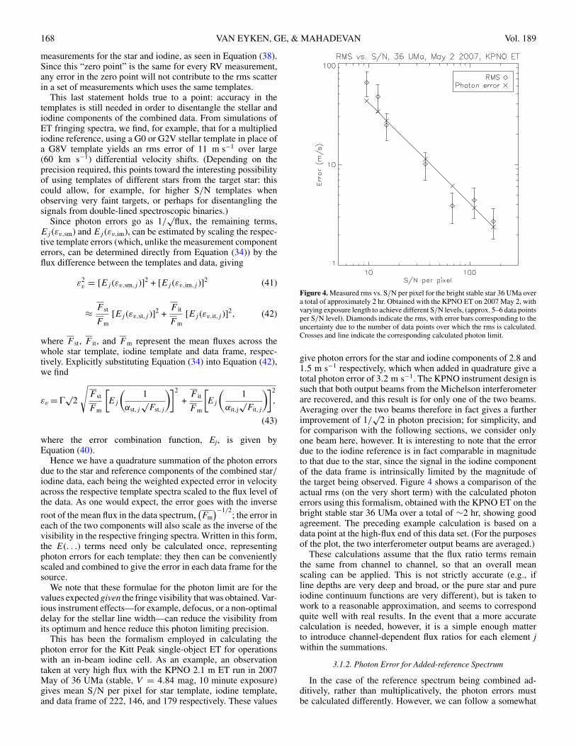
for the optical design. It is entirely reasonable to conceiveof a photon-limited DFDI-type instrument. However, even incases where photon noise is dominated by other effects in thevery high precision regime, photon noise inevitably becomessignificant at the faint end of the stellar target sample. Forthe MARVELS/Keck ET, geared toward moderate precisionsurveys of fainter targets, although other errors dominate theinstrument requirements error budget at the brightest (V ∼8 mag) end of the target range, photon noise becomes asignificant part of the error at fainter levels (down to V =12 mag, ∼21.5 m s−1 of a total 35.0 m s−1; see Ge et al.2009). In the high precision, high-flux regime (e.g., a planned1 m s−1—level cross-dispersed DFDI upgrade for the KPNOET), the photon error is also important as it indicates the levelbelow which other sources of systematic and random error mustbe driven.
The photon error in the phase measurement (and hencevelocity measurement) from a single channel can be estimatedfollowing Ge (2002). This gives essentially
εv,j ≈ 1
π√
2
cλ
dαj
√Fj
= Γ√
2
αj
√Fj
, (34)
where εv,j is the error in velocity due to channel j alone, c isthe speed of light, λ is the wavelength, d is the optical delay, αj
is the visibility of the fringe, Fj is the total flux in the channel,and Γ is the usual phase–velocity scaling factor (Equation (11),ignoring the negative sign since we are interested only in themagnitude).11 The terms following the Γ represent the error inphase due to the photon noise, εφ,j = √
2/(αj
√Fj ). Following
a similar derivation, it is straightforward to show that the errorin visibility due to photon noise, εα,j , is given by
εα,j =√
2
Fj
, (35)
and hence, assuming independent errors, there is a useful simplerelationship between the errors in phase and visibility:
εφ,j = εα,j
αj
. (36)
11 The small difference in the numerical factor in the denominator ofEquation (34) (π
√2 versus 4) is due to using the rms slope of the fringe, rather
than the mean absolute slope used in Ge (2002). Monte Carlo simulations ofsinusoid fits suggest that the rms slope gives more accurate results.
As a general rule, we can see from Equation (34) that precisiongoes with the inverse root of flux, as one would expect, and alsoas the inverse of visibility: higher flux and/or higher visibilitymean better precision. From this formula we can derive thephoton errors in the final differential RV for different calibrationscenarios.
For simplicity in the following formulae, we take λ to beconstant, taking the wavelength value at the center of thespectrum, since it varies by only ∼10% from one end of thespectrum to the other in the current ET instruments. For aninstrument with a very large bandwidth, however, it may benecessary to consider it properly as a function of channel, λj .This simply means it cannot be taken outside the brackets asin the following derivations, but otherwise the formalism is thesame.
3.1.1. Photon Error for Multiplied Reference
To calculate the expected error in an RV measurement for asingle data frame, assuming an instrument configuration wherean iodine or other reference spectrum multiplies the input stellarspectrum, we consider the resulting data spectrum as consistingof two components, a star component and an iodine component.The calculated phase shift due to intrinsic target Doppler shift,Δφ is given by
Δφ = 〈φsm,j − φst,j 〉 − 〈φim,j − φit,j 〉, (37)
where 〈. . .〉 here represents a weighted mean over all j, φsm,j andφim,j represent the phases for the star and iodine componentsof the combined star/iodine data (“measurement”) frame, andφst,j and φit,j are the phases measured in the separate purestar and iodine templates. For convenience, we immediatelymap these phases to corresponding “velocity” measurements bymultiplying both sides by Γ to give a velocity shift, Δv (thoughwith the caveat that a velocity measurement of a single channelin a single spectrum has no physical meaning in itself until it isdifferenced with another spectrum):
Δv = 〈vsm,j − vst,j 〉 − 〈vim,j − vit,j 〉. (38)
Using εv with corresponding subscripts to represent the variouserrors in this equation, we can expect a total photon error in Δvto be given by
ε2v = [
Ej
(√ε2v,sm,j + ε2
v,st,j
)]2+
[Ej
(√ε2v,im,j + ε2
v,it,j
)]2,
(39)where Ej (σ ) represents the standard statistical error in aweighted mean:
Ej (σj ) ≡ 1√∑j 1/σ 2
j
. (40)
In practice, the two template terms in Equation (39) areneglected, for two reasons. The first is simply because in generalthe templates will have significantly higher flux than the dataframe: the iodine template can be taken with arbitrarily highflux since it is obtained with a quartz lamp as a source; and thestellar template is usually deliberately taken with higher fluxthan the data so that it does not compromise the entire data set.The second reason is a little more subtle. All RV measurementswith this kind of instrument are differential, measured relativeto the two templates which effectively set the zero point of the
168 VAN EYKEN, GE, & MAHADEVAN Vol. 189
measurements for the star and iodine, as seen in Equation (38).Since this “zero point” is the same for every RV measurement,any error in the zero point will not contribute to the rms scatterin a set of measurements which uses the same templates.
This last statement holds true to a point: accuracy in thetemplates is still needed in order to disentangle the stellar andiodine components of the combined data. From simulations ofET fringing spectra, we find, for example, that for a multipliediodine reference, using a G0 or G2V stellar template in place ofa G8V template yields an rms error of 11 m s−1 over large(60 km s−1) differential velocity shifts. (Depending on theprecision required, this points toward the interesting possibilityof using templates of different stars from the target star: thiscould allow, for example, for higher S/N templates whenobserving very faint targets, or perhaps for disentangling thesignals from double-lined spectroscopic binaries.)
Since photon errors go as 1/√
flux, the remaining terms,Ej (εv,sm) and Ej (εv,im), can be estimated by scaling the respec-tive template errors (which, unlike the measurement componenterrors, can be determined directly from Equation (34)) by theflux difference between the templates and data, giving
ε2v = [Ej (εv,sm,j )]2 + [Ej (εv,im,j )]2 (41)
≈ F st
F m[Ej (εv,st,j )]2 +
F it
F m[Ej (εv,it,j )]2, (42)
where F st, F it, and F m represent the mean fluxes across thewhole star template, iodine template and data frame, respec-tively. Explicitly substituting Equation (34) into Equation (42),we find
εv = Γ√
2
√F st
F m
[Ej
(1
αst,j√
Fst,j
)]2
+F it
F m
[Ej
(1
αit,j√
Fit,j
)]2
,
(43)
where the error combination function, Ej, is given byEquation (40).
Hence we have a quadrature summation of the photon errorsdue to the star and reference components of the combined star/iodine data, each being the weighted expected error in velocityacross the respective template spectra scaled to the flux level ofthe data. As one would expect, the error goes with the inverse
root of the mean flux in the data spectrum,(Fm
)−1/2; the error in
each of the two components will also scale as the inverse of thevisibility in the respective fringing spectra. Written in this form,the E(. . .) terms need only be calculated once, representingphoton errors for each template: they then can be convenientlyscaled and combined to give the error in each data frame for thesource.
We note that these formulae for the photon limit are for thevalues expected given the fringe visibility that was obtained. Var-ious instrument effects—for example, defocus, or a non-optimaldelay for the stellar line width—can reduce the visibility fromits optimum and hence reduce this photon limiting precision.
This has been the formalism employed in calculating thephoton error for the Kitt Peak single-object ET for operationswith an in-beam iodine cell. As an example, an observationtaken at very high flux with the KPNO 2.1 m ET run in 2007May of 36 UMa (stable, V = 4.84 mag, 10 minute exposure)gives mean S/N per pixel for star template, iodine template,and data frame of 222, 146, and 179 respectively. These values
Figure 4. Measured rms vs. S/N per pixel for the bright stable star 36 UMa overa total of approximately 2 hr. Obtained with the KPNO ET on 2007 May 2, withvarying exposure length to achieve different S/N levels, (approx. 5–6 data pointsper S/N level). Diamonds indicate the rms, with error bars corresponding to theuncertainty due to the number of data points over which the rms is calculated.Crosses and line indicate the corresponding calculated photon limit.
give photon errors for the star and iodine components of 2.8 and1.5 m s−1 respectively, which when added in quadrature give atotal photon error of 3.2 m s−1. The KPNO instrument design issuch that both output beams from the Michelson interferometerare recovered, and this result is for only one of the two beams.Averaging over the two beams therefore in fact gives a furtherimprovement of 1/
√2 in photon precision; for simplicity, and
for comparison with the following sections, we consider onlyone beam here, however. It is interesting to note that the errordue to the iodine reference is in fact comparable in magnitudeto that due to the star, since the signal in the iodine componentof the data frame is intrinsically limited by the magnitude ofthe target being observed. Figure 4 shows a comparison of theactual rms (on the very short term) with the calculated photonerrors using this formalism, obtained with the KPNO ET on thebright stable star 36 UMa over a total of ∼2 hr, showing goodagreement. The preceding example calculation is based on adata point at the high-flux end of this data set. (For the purposesof the plot, the two interferometer output beams are averaged.)
These calculations assume that the flux ratio terms remainthe same from channel to channel, so that an overall meanscaling can be applied. This is not strictly accurate (e.g., ifline depths are very deep and broad, or the pure star and pureiodine continuum functions are very different), but is taken towork to a reasonable approximation, and seems to correspondquite well with real results. In the event that a more accuratecalculation is needed, however, it is a simple enough matterto introduce channel-dependent flux ratios for each element jwithin the summations.
3.1.2. Photon Error for Added-reference Spectrum
In the case of the reference spectrum being combined ad-ditively, rather than multiplicatively, the photon errors mustbe calculated differently. However, we can follow a somewhat
No. 1, 2010 THEORY OF DFDI FOR RADIAL VELOCITY EXOPLANET SEARCHES 169
similar approach. Again, we consider the errors due to star andiodine components of the combined star/iodine data, and neglectthe errors due to the templates, so that, as for Equation (41):
ε2v = [Ej (εv,sm,j )]2 + [Ej (εv,im,j )]2, (44)
where Ej is again defined as in Equation (40). The individualcomponents εv,sm,j and εv,im,j must be reevaluated, however,since the photon noise from the two separate sources willnow combine additively (for example, if one of the sourcesis considerably brighter than the second, its photon noise willdominate over the signal in the second). We can think of aneffective visibility for the two components in the combined data,αsm,j and αim,j . Remembering that fringe amplitude is given bythe product of the visibility and the mean flux in the fringe, wecan write
αsm,jFm,j = αst,jAsFst,j ; αim,jFm,j = αit,jAiFit,j , (45)
where αst,j and αit,j are the fringe visibilities for channel j inthe star and iodine templates respectively; and Fst,j , Fit,j , andFm,j are the mean fluxes across the channel for the star template,iodine template, and data (measurement) frame, respectively. Asand Ai are wavelength-independent scaling factors that allow forflux differences between the templates and the respective datacomponents, as in Section 2.6.2. Hence we find
αsm,j = αst,jAsFst,j
Fm,j
; αim,j = αit,jAiFit,j
Fm,j
, (46)
where Fst,j and Fit,j are the total fluxes across the channelfor the star and iodine templates, and Fm,j is the total fluxin the channel for the data frame. Substituting these effectivevisibilities in Equation (34) gives
εv,sm,j = Γ√
2
√Fm,j
αst,jAsFst,j
εv,im,j = Γ√
2
√Fm,j
αit,jAiFit,j. (47)
Using these we can now evaluate Equation (44) to obtain anestimate of the photon limiting error, so that
εv = Γ√
2
√[Ej
( √Fm,j
αst,jAsFst,j
)]2
+
[Ej
( √Fm,j
αit,jAiFit,j
)]2
,
(48)where, due to flux conservation, As and Ai are subject to theconstraint:
AsFst,j + AiFit,j = Fm,j . (49)
Again we have found a quadrature summation of errorsdue to the star and reference components, scaled to matchthe respective component fluxes in the data, very similar toEquation (43). However, in this case, the scaling factors, As andAi, must be determined as parameters during the velocity shiftsolution, and AsFst,j and AiFit,j represent the fluxes in the starand iodine components of the data, respectively.
This time, we do not attempt to assume channel-independentflux ratios. This is because for additively combined referencesit becomes possible to consider using emission spectra (e.g.,a ThAr lamp) as the reference, rather than the usual iodineabsorption spectrum. Clearly the flux ratio between data and
reference template frames is very different for regions wherethere are no reference emission lines compared with those whereemission lines are present. It is therefore not reasonable to takethe flux terms outside the summation in the error combinationfunction Ej.
To gain a handle on the behavior of Equation (48), we can seethat if we consider only a single channel, so that for a functionf, E(f ) → f , and assume both that the source and referencevisibilities are roughly equal (reasonable for star and iodine, toorder of magnitude) and that the total flux Fm remains constant,then to minimize the total error, we need only to minimizethe function: (AsFst,j )−2 + (AiFit,j )−2. Given the constraint ofEquation (49) it is straightforward to show that this is minimizedwhen AsFst,j = AiFit,j , in other words, when the componentstar and iodine fluxes are approximately equal. When eithercomponent has a very small flux compared with the other, oneor other of the terms in Equation (48) will become very large.Broadly speaking, then, we can see that the fluxes of star andreference need to be balanced in order to minimize photon error.
In practice, rather than the total flux being constant, it isof more interest to hold the stellar component constant andvary the reference component to find the optimum; using realspectra, and allowing differing visibilities, the balance pointbecomes a little skewed from unity. The exact optimal balancepoint depends on the spectra in question. Allowing for thegain in optical throughput from losing the absorption in thegas cell reference, this equation at its balance point generallygives photon errors on a similar level to the photon errorsfor a multiplied iodine reference, if we use iodine spectra asreferences in both cases (i.e., tungsten-illuminated iodine inthe added-reference scheme). Using the same observations asin Section 3.1.1 to calculate error estimates as if the spectrahad been added, and assuming that the flux level of the star inthe template and the hypothetical combined observation is thesame, we find an optimal ratio of iodine to star flux of 0.96and a total photon error of 3.6 m s−1, comprised of iodine andstar component errors of 3.1 m s−1 and 1.8 m s−1, compared tothe total error of 3.2 m s−1 for multiplied spectra. That the twoare similar is not surprising: adding a reference spectrum to thestellar spectrum at a matching flux level will approximatelyhalve fringe visibility and hence double the error, but alsodouble the flux, reducing the error by 1/
√2, giving a total√
2 increase in the error size. This coincidentally matches theincrease in error size for in-beam-iodine calibration due to thefact that the iodine typically absorbs ∼50% of the incidentlight. (The slight mismatch in the figures calculated is due tothe fact that in the multiplicative case, the combined data frameactually had particularly high flux, probably because of bettersky transparency at the time the frame was taken than when thetemplate was taken).
The above argument holds true for iodine since the continuumshape and fringe visibilities are broadly similar to those of thestellar spectrum. If we instead use a ThAr emission spectrumfor the added reference, we appear to perform even rather betterthan the in-beam iodine case: the same calculations as abovewith a ThAr spectrum replacing the iodine spectrum yield atotal photon error of 2.5 m s−1, with star and ThAr componentsof 2.4 m s−1 and 0.65 m s−1 respectively (with an optimum ratioof mean fluxes of 0.26—now substantially different because ofthe very different nature of an emission spectrum). ThAr alsoshows a weaker dependence on relative flux level, which givesit an advantage in terms of practical application since less effortwould need to be expended on matching the brightness to each

170 VAN EYKEN, GE, & MAHADEVAN Vol. 189
target observation. This is likely because most of the Dopplerinformation is primarily concentrated in a few bright lines inthe ThAr, where it is spread more broadly across the stellarspectrum. Where the ThAr lines are strong, the stellar Dopplerinformation is likely largely lost due to the added photon noise.However, since there are relatively few such lines, there is nottoo much impact on the total stellar Doppler information, andincreasing the ThAr flux does not make as large a difference asfor the case of an iodine spectrum. We note, however, that atvery high flux levels, saturation of the brightest ThAr emissionlines is likely to complicate this analysis somewhat.
Added-beam reference calibration provides one possiblesolution to the reference addition approximation error discussedin Section 3.3.3, and the discussion here should provide aformalism for calculating the photon errors. Such a calibrationapproach, however, has not yet been attempted within the ETprogram, although basic simulations bear out these calculations.
3.1.3. Photon Error with a Separate Reference
Finally we consider the simple case where there is no simulta-neous common-path reference, but rather a reference separatedeither spatially or in time. Once again, we find a weighted meanvelocity shift between (now pure) star measurement and somereference star template, and the same between a pure referencespectrum measurement and a corresponding template. (The ref-erence need not be iodine, but we retain the “i” subscript notationfor consistency). The results are differenced to obtain a correctedintrinsic stellar Doppler shift. If we neglect the template errorsas before, then the photon errors for the data frame are foundagain similarly to Equation (41):
ε2v = [Ej (εv,s,j )]2 + [Ej (εv,i,j )]2. (50)
The difference is that here we use subscripts “s” and “i,” ratherthan “sm” and “im,” to indicate that we are no longer looking atcomponents of a combined reference/star measurement frame,but at pure star and pure reference measurements, respectively.Again substituting the basic photon error Equation (34), weobtain
εv = Γ√
2
√[Ej
(1
αs,j√
Fs,j
)]2
+
[Ej
(1
αi,j√
Fi,j
)]2
.
(51)The form of the equation is now much simpler, since no flux
or visibility scaling is required. Errors again go as the inverseof the visibilities of star and iodine, and as the inverse root ofthe flux. It may also be the case (indeed, observations shouldbe taken such that it is the case) that the reference spectrum hassignificantly higher S/N, and therefore its photon errors can beneglected, so that only the first error combination term in thesquare root remains.
Taking our same data and templates once again, we cancalculate a hypothetical photon error for comparison: this time,using iodine as a separate reference yields a total error of2.9 m s−1 comprising star and iodine components of 2.3 m s−1
and 1.9 m s−1 respectively (note that the iodine error level hereis relatively high in comparison to the star component: this ispurely because of the exceptionally high flux from the star inthese particular observations); using ThAr instead yields a totalerror of 2.4 m s−1, with star and ThAr components of 2.3 m s−1
and 0.77 m s−1 (though again we have not included the effectsof saturation in the ThAr calculation, which may increase theThAr errors somewhat).
Figure 5. Fringe along one channel due to source (upper curve) and contami-nating low flux fringe (lower curve). Measured fringe is a summation of thesetwo fringes.
This approach is appropriate to the MARVELS/Keck ET,where pure star science exposures are bracketed in time withpure iodine reference exposures, and the instrument is highlystabilized in both pressure and temperature. The baseline designrequirements anticipate a photon error of 3.5 m s−1 at V =8 mag, and 21.5 m s−1 at V = 12 mag (see Section 4.4 and Geet al. 2009).
3.2. Additive Contaminating Spectra
It is often useful to be able to calculate a rough estimate ofthe errors due to contaminating additive background spectra.We derive a formalism for doing so here. This formalismwill enable us to calculate the effect of background moonlightcontamination, contaminating background stars, or double-linedspectroscopic binaries, for example. In addition, we will thenbe able to extend the formalism to treat multiplicative (i.e.,flux independent) contaminants, such as any residual unfilteredcomb presence or the iodine/star cross-talk term that causes thereference addition approximation error, and try to assess theirrelative significance.
3.2.1. Derivation
Figure 5 shows a fringe along one detector column (in the slitdirection) due to the target source alone, with fringe amplitudeas, mean flux Fs, and phase φs. For simplicity we assume noiodine fiducial reference, since we are only aiming for an order-of-magnitude estimate. A second contaminating fringe of loweramplitude ac and mean flux Fc due to background contaminationis also shown, with phase φc. If the spatial frequency of thefringes is f, then the summation of these two fringes will givethe total (also sinusoidal) measured fringe:
Fs + �{asei(f x+φs)} + Fc + �{ace
i(f x+φc)}= Fs + Fc + �{ase
i(f x+φs) + acei(f x+φc)}, (52)
where x identifies position along the slit. Fs + Fc represents themean value of the measured flux. The last term represents thevarying sinusoidal net fringe.
We are interested in the phase error, εφ , introduced intothe measured fringe by the contaminating spectrum. Since weare only interested in the phase information, we ignore theoffset term Fs + Fc, and represent the varying term as a vectorsummation, as shown in Figure 6, where as and ac representthe source and contaminant fringe amplitudes as before. The
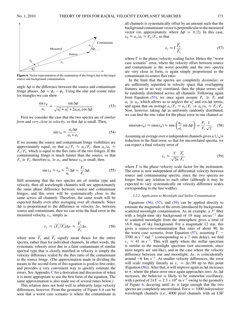
No. 1, 2010 THEORY OF DFDI FOR RADIAL VELOCITY EXOPLANET SEARCHES 171
εφ
φs
Δφ
Source
s
Contaminant
Measuredc
a
a
Figure 6. Vector representation of the summation of the fringes due to the targetsource and background contamination.
angle Δφ is the difference between the source and contaminantfringe phases, Δφ = φc − φs. Using the sine and cosine rulesfor triangles we can show
sin εφ
ac= sin Δφ√
a2s + a2
c + 2asac cos Δφ. (53)
First we consider the case that the two spectra are of similarform and very close in velocity, so that Δφ is small. Then,
sin εφ ≈ acΔφ
as + ac. (54)
If we assume the source and contaminant fringe visibilities areapproximately equal, so that as/Fs ≈ ac/Fc, then ac/as ≈Fc/Fs, which is equal to the flux ratio of the two fringes. If thecontaminating fringe is much fainter than the source, so thatFs � Fc, therefore as � ac, and hence εφ is small, then
sin εφ ≈ εφ ≈ ac
asΔφ = Fc
FsΔφ. (55)
Still assuming that the two spectra are of similar type andvelocity, then all wavelength channels will see approximatelythe same phase difference between source and contaminantfringes, and this error will be systematically close to thesame across all channels. Therefore, the same result will beexpected finally even after averaging over all channels. SinceΔφ is proportional to the difference in velocity, Δv, betweensource and contaminant, then we can write the final error in themeasured velocity, εv , simply as
εv ≈ (Fc/Fs)Δv ≈ Fc
FsΔv, (56)
where now Fc and Fs signify mean fluxes for the entirespectra, rather than for individual channels. In other words, thesystematic velocity error due to a faint contaminant of similarspectral type that is closely matched in velocity is simply thevelocity difference scaled by the flux ratio of the contaminantto the source fringe. (The approximation made in dividing themeans in the second form of this equation is good to first order,and provides a very convenient way to quickly estimate theerrors. See Appendix C for a derivation and discussion of whenit is more appropriate to use the first form of the equation. Thesame approximation is also made use of several times below.)
This relation does not hold well to arbitrarily large velocitydifferences, however. From the geometry of Figure 6 it can beseen that a worst case scenario is where the contaminant in
all channels is systematically offset by an amount such that thebackground contaminant vector is perpendicular to the measuredvector (or, approximately, where Δφ = π/2). In this case,εφ ≈ ac/as ≈ Fc/Fs, so that
εv ≈ ΓFc
Fs, (57)
where Γ is the phase/velocity scaling factor. Hence the “worstcase scenario” error, where the velocity offset between sourceand contaminant is the worst possible and the two spectraare very close in form, is again simply proportional to thecontaminant-to-source flux ratio.
In the limit that the spectra are completely dissimilar, orare sufficiently separated in velocity space that overlappingfeatures are in no way correlated, then the phase errors willbe randomly distributed across all channels. Following againfrom Equation (53), we once again assume Fs � Fc andas � ac, which allows us to neglect the a2
c and cos Δφ terms;and again that on average as/Fs ≈ ac/Fc ⇒ ac/as ≈ Fc/Fs.Now, however, taking Δφ as uniformly randomly distributed,we can find the rms value for the phase error in one channel as
rms(sin εφ) ≈ rms(εφ) ≈ rms
(ac
assin Δφ
)= Fc
Fs
1√2. (58)
Assuming an average over n independent channels gives a 1/√
nreduction in the final error, so that for uncorrelated spectra, wecan expect a final velocity error of
εv ≈ Γ√2n
Fc
Fs, (59)
where Γ is the phase–velocity scale factor for the instrument.The error is now independent of differential velocity betweensource and contaminating spectra, since the two spectra nolonger bear any relation to each other (although it may beexpected to vary systematically on velocity difference scalescorresponding to the line widths).
3.2.2. Application to Moonlight and Stellar Contamination
Equations (56), (57), and (59) can be applied directly toestimate the magnitude of the errors introduced by background-scattered moonlight contamination. As an example, a 3′′ fiberwith a bright-time sky background of 19 mag arcsec−2 dueto scattered moonlight from the atmosphere gives a total of16.9 mag of sky background. For a magnitude 12 star, thisgives a source-to-contamination flux ratio of about 90. Inthe worst case scenario, from Equation (57), assuming Γ ∼3700 m s−1 rad−1 (corresponding to a 7 mm delay), we findεv ≈ 41 m s−1. This will apply where the stellar spectrumis similar to the moonlight spectrum (not uncommon, sincemost targets are sun-like), and in the case where the velocitydifference between star and moonlight, Δv, is coincidentallyaround ∼6 km s−1. At smaller velocity differences, the errorwill scale roughly linearly as εv = Δv/90 up to this point(Equation (56)). After that, it will improve again as Δφ increasesto π , where the phase error once again approaches zero. As Δφincreases, the behavior is likely to be somewhat oscillatory,with a period of 2πΓ = 2.3 × 10⁴ m s−1 owing to the geometryof Figure 6, decaying until Δv is large enough that the twospectra are completely uncorrelated. For n = 1000 independentwavelength channels (i.e., 4000 pixel channels with an LSF

172 VAN EYKEN, GE, & MAHADEVAN Vol. 189
Figure 7. Simulations of moonlight contamination, showing the systematic error introduced by contaminating moonlight at 19 mag arcsec−2 for a V = 12 F9V staron a 3′′ fiber, as a function of velocity difference between target star and moon spectrum.
∼4 pixels wide), the error should then approach Equation (59),with an rms value of around εv ≈ 0.8 m s−1. This should alsobe the typical error size when the star and moon spectra are verydifferent in form.
Simulations of the effect of moonlight contamination showreasonable agreement: Figure 7 shows the RV deviation causedby synthetic moonlight contamination added to a syntheticstellar spectrum, and then multiplied by the interferometerresponse function and degraded in resolution to simulate realinstrument spectra (ignoring the iodine reference). The resultingspectra are run through the standard ET reduction pipeline toassess the effects of the contamination.
The instrument parameters given here are chosen to matchthe parameters of the simulation, which reflect a typical ET-likeinstrument design. For comparison, the MARVELS/Keck ETin fact uses 1.′′8 fibers, with Γ ∼ 3400 m s−1 rad−1, leading toa worst-case error of only 14 m s−1, at the faintest end of theMARVELS range. Reducing the fiber size is clearly one effec-tive way of mitigating the effect of moonlight contamination,although this may be at the expense of throughput if telescopeguiding or seeing is not optimal. Reduction of moon contami-nation error is discussed further in Section 4.1.
In exactly the same way, we can calculate the effects ofcontamination by a background star: for example, a backgroundstar of the same spectral type and class, but 5 mag fainter(i.e., fainter by a flux ratio of 100) would give about thesame level of error. At increasingly different spectral types,the contaminant star will cause less of a problem as the spectrabecome less correlated. Hence for a faint companion (as opposedto background) star, although the flux ratio may be higher, the
effect will be at least partially mitigated by the difference inspectral type.
3.3. Multiplicative Fringe Contamination
In addition to additive contaminating spectra, certain errorscan appear as multiplicative effects in the fringing spectra.These are independent of flux and correspond more closelyto fringe errors rather than flux errors in the spectra. Residualinterferometer comb, for example, will behave in this way (aconcern for multiplied-reference modes of operation), and thecross-talk term from the reference addition approximation canalso be considered in the same way.
3.3.1. Derivation
We can follow the same formalism as for background spec-trum contamination. In this case, however, instead of the sourceand contaminant fringe visibilities being similar, the fluxesare similar, so that Fs ≈ Fc. Dividing the denominators ofEquation (53) through by Fs ≈ Fc, we can replace the fringeamplitudes as and ac with their respective visibilities αs ≡ as/Fsand αc ≡ ac/Fc. The source spectrum and interferometer combare completely unrelated in form. Assuming αc αs we canfollow the same reasoning as for Equation (59) and write
εv ≈ Γ√2n
αc
αs, (60)
where αc and αs are representative visibilities for the entire con-taminant and source spectra respectively (again see Appendix C

No. 1, 2010 THEORY OF DFDI FOR RADIAL VELOCITY EXOPLANET SEARCHES 173
regarding the division of means here). The error is now propor-tional to the ratio of visibilities, and again decreases with theroot of the number of spectral channels, n.
3.3.2. Application to Residual Interferometer Comb
As an example application, we can consider the effectof residual interferometer comb. For the case of using amultiplied fiducial spectrum such as in-beam iodine absorption,if the interferometer comb (Section 2.4) is not completelyremoved—either by careful tuning of interferometer delay andslit width or by Fourier filtering in the data processing—then itacts as contaminating fringes. In order for the reference additionapproximation to work, the comb term in Equation (22) mustbe completely removed (see the subsequent discussion). Thishas in the past been an issue with some configurations of theET instruments, for example: in these cases the sampling by theresolution element was such that the comb was aliased in places,creating a low-frequency pattern in the dispersion directionwhich was impossible to filter out without losing significantDoppler information.
Here, it is appropriate to take the combined star/iodine dataas the source spectrum, since the comb error arises in theformula for the combined data (Equation (22)). A residual combvisibility of 0.5% (cf. ∼1% comb visibility in unfiltered KPNOET data) on top of a spectrum of typical mean visibility of say,4%, and taking the KPNO ET value of Γ ∼ 3300 m s−1 rad−1
with n = 1000 independent channels, would give an expectederror of εv ≈ 9 m s−1.
In practice, however, we have found that, provided combaliasing is avoided in the instrument design and alignment,removing the interferometer comb during image preprocessingwith a simple one-dimensional low-pass Fourier filter appearsto be effective in completely mitigating this error. The combcannot be measured or seen by eye above the photon noise infiltered continuum lamp spectra, and we have not yet found anyevidence of residual comb causing problems in the final data.
3.3.3. Application to the Addition Approximation
In order to estimate the errors introduced by the additionapproximation discussed in Section 2.6.1, we can also followa similar approach, treating the cross term from Equation (22)which is ignored in the approximation (or rather, treating thelack of cross term) as if it were a contaminating spectrum. First,we consider the simplified case of two discrete overlappingGaussian absorption lines, from template spectra labeled A andB (e.g., an iodine and a stellar line), combined by multiplicationto give the measured spectrum, labeled M. Both line centers areexactly coincident. The fractional line depths are representedby D (0 � D � 1), with corresponding subscripts a, b, and m.From Ge (2002), we have that in general
α = De−3.56d2/l2c ≡ KD, (61)
where α is the absolute fringe visibility (so that the complexvisibility is α = αeiφ as usual), d is the interferometer delay,lc = λ2/Δλ is the coherence length of the interferometer beamwith line width Δλ at wavelength λ, and K = exp(−3.56d2/l2
c )is a constant (for a given wavelength). Although not veryrealistic, we begin by assuming both lines A and B and theresulting line M are of similar width, and that the measuredline, which is the product of the two lines, is also approximatelyGaussian. K is then approximately the same for all three lines.
Summation approximation
α + αb
αm
αε
φε
εφ
φ
True
Error term
a
Figure 8. Vector representation of the summation of the true complex visibilityand the error term due to the addition approximation.
We can then write
αm ≈ DmK = [1 − (1 − Da)(1 − Db)]K
= [Da + Db − DaDb]K
= αa + αb − DaDbK. (62)
In the addition approximation, the complex visibilities of thetemplate spectra are added together. In this simple case, the twolines are centered at the same wavelength and both are Gaussian,so that one line is simply a scaled version of the other. By thelinearity of Fourier transforms, this means that the phases ofthe two complex visibilities must be identical, so that in theaddition approximation, the two absolute visibilities add to giveαm ≈ αa + αb. The remaining term in Equation (62) is thereforeapproximately the error, αε, the difference between the addedtemplates and the actual measured visibility:
αε = DaDbK. (63)
In the more general case that the two line centers are notexactly coincident or the same shape, so that the respectivetemplate fringes are not in phase, the error term will also includea phase difference, becoming a two-dimensional vector, αεe
iφε .Taking the error term above as a reasonable estimate of thelength of this vector and assuming φε is uniformly randomlydistributed, we can calculate a corresponding representativeerror in phase of the summation approximation. Figure 8 showsthe addition of the “true” (measured) complex visibility andthe error term to give the solution according to the summationapproximation. φ represents the phase of the true complexvisibility, and εφ represents the error in the measurement of thatphase. If we assume the resulting measured visibility vectorsand the error terms are uncorrelated from channel to channel,and if we take Da and Db to be some kind of representativeaverage line depth for the two spectra across all j, we can derivethe typical expected velocity error following the same reasoningas for Equation (60) and write
εv = Γ√2n
αε
αm
= Γ√2n
DaDb
Da + Db − DaDb, (64)
where n is again the number of independent channels, and theconstant K cancels. (Note that although angles φε in Figure 8and Δφ in Figure 6 are measured from different origins, theyare in both cases taken to be uniformly randomly distributedbetween 0 and 2π , so that the same reasoning applies for both.)
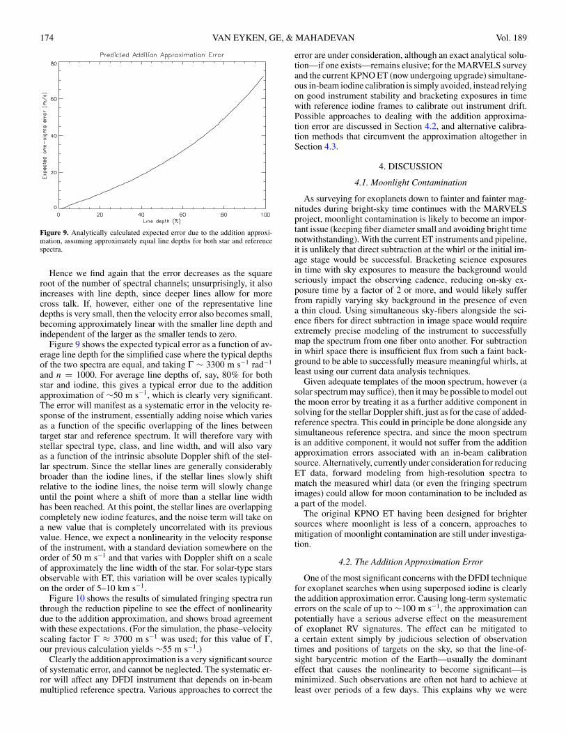
174 VAN EYKEN, GE, & MAHADEVAN Vol. 189
Figure 9. Analytically calculated expected error due to the addition approxi-mation, assuming approximately equal line depths for both star and referencespectra.
Hence we find again that the error decreases as the squareroot of the number of spectral channels; unsurprisingly, it alsoincreases with line depth, since deeper lines allow for morecross talk. If, however, either one of the representative linedepths is very small, then the velocity error also becomes small,becoming approximately linear with the smaller line depth andindependent of the larger as the smaller tends to zero.
Figure 9 shows the expected typical error as a function of av-erage line depth for the simplified case where the typical depthsof the two spectra are equal, and taking Γ ∼ 3300 m s−1 rad−1
and n = 1000. For average line depths of, say, 80% for bothstar and iodine, this gives a typical error due to the additionapproximation of ∼50 m s−1, which is clearly very significant.The error will manifest as a systematic error in the velocity re-sponse of the instrument, essentially adding noise which variesas a function of the specific overlapping of the lines betweentarget star and reference spectrum. It will therefore vary withstellar spectral type, class, and line width, and will also varyas a function of the intrinsic absolute Doppler shift of the stel-lar spectrum. Since the stellar lines are generally considerablybroader than the iodine lines, if the stellar lines slowly shiftrelative to the iodine lines, the noise term will slowly changeuntil the point where a shift of more than a stellar line widthhas been reached. At this point, the stellar lines are overlappingcompletely new iodine features, and the noise term will take ona new value that is completely uncorrelated with its previousvalue. Hence, we expect a nonlinearity in the velocity responseof the instrument, with a standard deviation somewhere on theorder of 50 m s−1 and that varies with Doppler shift on a scaleof approximately the line width of the star. For solar-type starsobservable with ET, this variation will be over scales typicallyon the order of 5–10 km s−1.
Figure 10 shows the results of simulated fringing spectra runthrough the reduction pipeline to see the effect of nonlinearitydue to the addition approximation, and shows broad agreementwith these expectations. (For the simulation, the phase–velocityscaling factor Γ ≈ 3700 m s−1 was used; for this value of Γ,our previous calculation yields ∼55 m s−1.)
Clearly the addition approximation is a very significant sourceof systematic error, and cannot be neglected. The systematic er-ror will affect any DFDI instrument that depends on in-beammultiplied reference spectra. Various approaches to correct the
error are under consideration, although an exact analytical solu-tion—if one exists—remains elusive; for the MARVELS surveyand the current KPNO ET (now undergoing upgrade) simultane-ous in-beam iodine calibration is simply avoided, instead relyingon good instrument stability and bracketing exposures in timewith reference iodine frames to calibrate out instrument drift.Possible approaches to dealing with the addition approxima-tion error are discussed in Section 4.2, and alternative calibra-tion methods that circumvent the approximation altogether inSection 4.3.
4. DISCUSSION
4.1. Moonlight Contamination
As surveying for exoplanets down to fainter and fainter mag-nitudes during bright-sky time continues with the MARVELSproject, moonlight contamination is likely to become an impor-tant issue (keeping fiber diameter small and avoiding bright timenotwithstanding). With the current ET instruments and pipeline,it is unlikely that direct subtraction at the whirl or the initial im-age stage would be successful. Bracketing science exposuresin time with sky exposures to measure the background wouldseriously impact the observing cadence, reducing on-sky ex-posure time by a factor of 2 or more, and would likely sufferfrom rapidly varying sky background in the presence of evena thin cloud. Using simultaneous sky-fibers alongside the sci-ence fibers for direct subtraction in image space would requireextremely precise modeling of the instrument to successfullymap the spectrum from one fiber onto another. For subtractionin whirl space there is insufficient flux from such a faint back-ground to be able to successfully measure meaningful whirls, atleast using our current data analysis techniques.
Given adequate templates of the moon spectrum, however (asolar spectrum may suffice), then it may be possible to model outthe moon error by treating it as a further additive component insolving for the stellar Doppler shift, just as for the case of added-reference spectra. This could in principle be done alongside anysimultaneous reference spectra, and since the moon spectrumis an additive component, it would not suffer from the additionapproximation errors associated with an in-beam calibrationsource. Alternatively, currently under consideration for reducingET data, forward modeling from high-resolution spectra tomatch the measured whirl data (or even the fringing spectrumimages) could allow for moon contamination to be included asa part of the model.
The original KPNO ET having been designed for brightersources where moonlight is less of a concern, approaches tomitigation of moonlight contamination are still under investiga-tion.
4.2. The Addition Approximation Error
One of the most significant concerns with the DFDI techniquefor exoplanet searches when using superposed iodine is clearlythe addition approximation error. Causing long-term systematicerrors on the scale of up to ∼100 m s−1, the approximation canpotentially have a serious adverse effect on the measurementof exoplanet RV signatures. The effect can be mitigated toa certain extent simply by judicious selection of observationtimes and positions of targets on the sky, so that the line-of-sight barycentric motion of the Earth—usually the dominanteffect that causes the nonlinearity to become significant—isminimized. Such observations are often not hard to achieve atleast over periods of a few days. This explains why we were
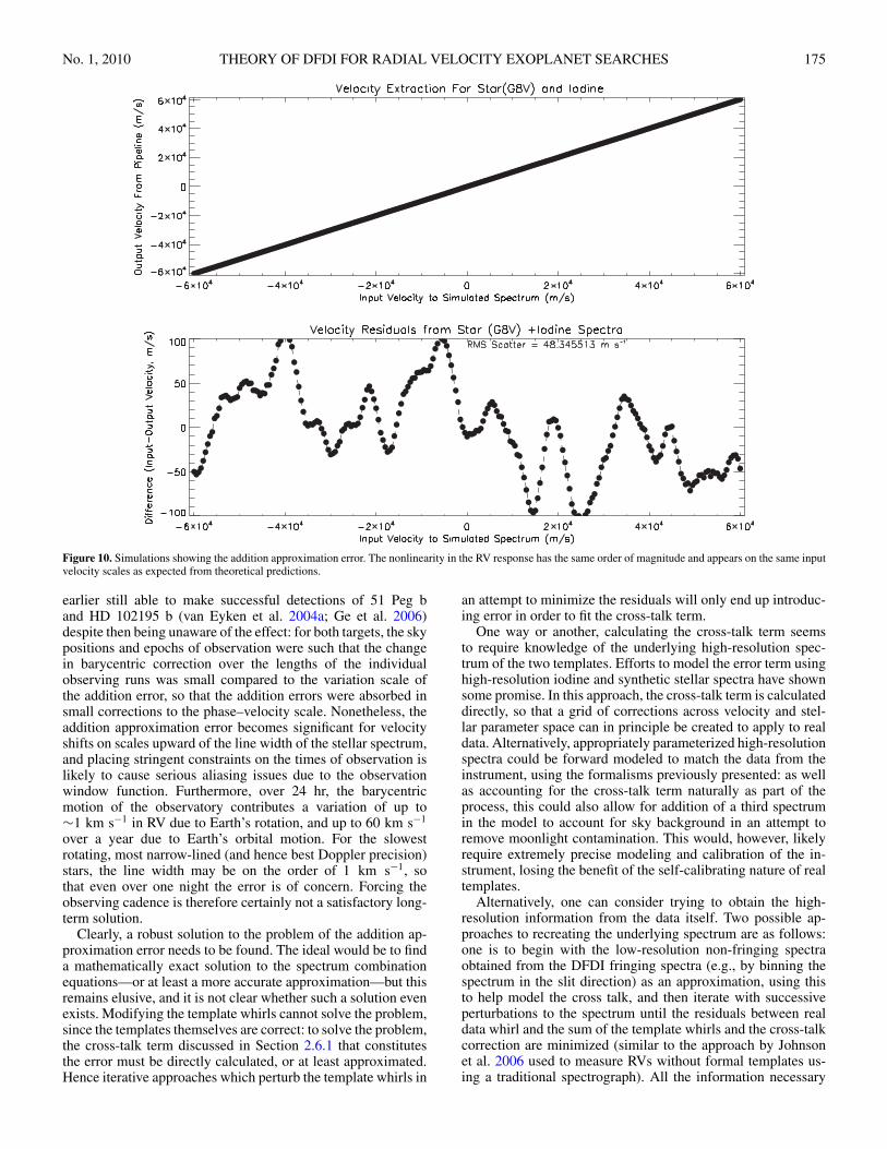
No. 1, 2010 THEORY OF DFDI FOR RADIAL VELOCITY EXOPLANET SEARCHES 175
Figure 10. Simulations showing the addition approximation error. The nonlinearity in the RV response has the same order of magnitude and appears on the same inputvelocity scales as expected from theoretical predictions.
earlier still able to make successful detections of 51 Peg band HD 102195 b (van Eyken et al. 2004a; Ge et al. 2006)despite then being unaware of the effect: for both targets, the skypositions and epochs of observation were such that the changein barycentric correction over the lengths of the individualobserving runs was small compared to the variation scale ofthe addition error, so that the addition errors were absorbed insmall corrections to the phase–velocity scale. Nonetheless, theaddition approximation error becomes significant for velocityshifts on scales upward of the line width of the stellar spectrum,and placing stringent constraints on the times of observation islikely to cause serious aliasing issues due to the observationwindow function. Furthermore, over 24 hr, the barycentricmotion of the observatory contributes a variation of up to∼1 km s−1 in RV due to Earth’s rotation, and up to 60 km s−1
over a year due to Earth’s orbital motion. For the slowestrotating, most narrow-lined (and hence best Doppler precision)stars, the line width may be on the order of 1 km s−1, sothat even over one night the error is of concern. Forcing theobserving cadence is therefore certainly not a satisfactory long-term solution.
Clearly, a robust solution to the problem of the addition ap-proximation error needs to be found. The ideal would be to finda mathematically exact solution to the spectrum combinationequations—or at least a more accurate approximation—but thisremains elusive, and it is not clear whether such a solution evenexists. Modifying the template whirls cannot solve the problem,since the templates themselves are correct: to solve the problem,the cross-talk term discussed in Section 2.6.1 that constitutesthe error must be directly calculated, or at least approximated.Hence iterative approaches which perturb the template whirls in
an attempt to minimize the residuals will only end up introduc-ing error in order to fit the cross-talk term.
One way or another, calculating the cross-talk term seemsto require knowledge of the underlying high-resolution spec-trum of the two templates. Efforts to model the error term usinghigh-resolution iodine and synthetic stellar spectra have shownsome promise. In this approach, the cross-talk term is calculateddirectly, so that a grid of corrections across velocity and stel-lar parameter space can in principle be created to apply to realdata. Alternatively, appropriately parameterized high-resolutionspectra could be forward modeled to match the data from theinstrument, using the formalisms previously presented: as wellas accounting for the cross-talk term naturally as part of theprocess, this could also allow for addition of a third spectrumin the model to account for sky background in an attempt toremove moonlight contamination. This would, however, likelyrequire extremely precise modeling and calibration of the in-strument, losing the benefit of the self-calibrating nature of realtemplates.
Alternatively, one can consider trying to obtain the high-resolution information from the data itself. Two possible ap-proaches to recreating the underlying spectrum are as follows:one is to begin with the low-resolution non-fringing spectraobtained from the DFDI fringing spectra (e.g., by binning thespectrum in the slit direction) as an approximation, using thisto help model the cross talk, and then iterate with successiveperturbations to the spectrum until the residuals between realdata whirl and the sum of the template whirls and the cross-talkcorrection are minimized (similar to the approach by Johnsonet al. 2006 used to measure RVs without formal templates us-ing a traditional spectrograph). All the information necessary
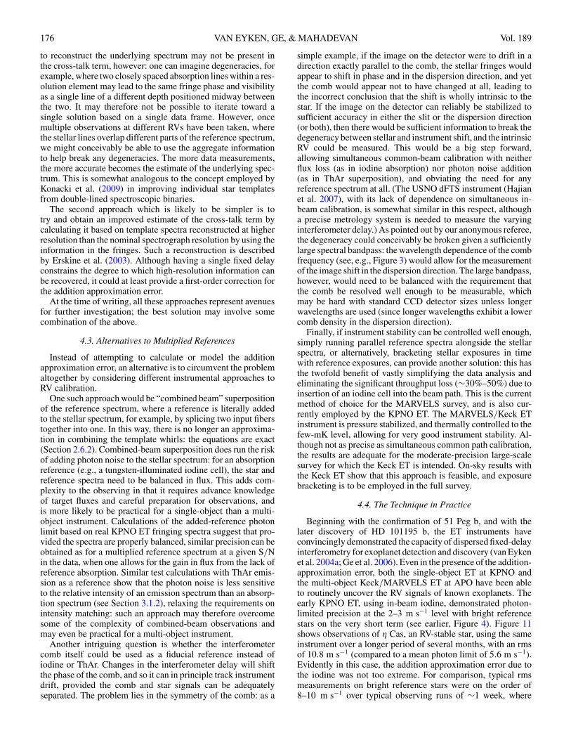
176 VAN EYKEN, GE, & MAHADEVAN Vol. 189
to reconstruct the underlying spectrum may not be present inthe cross-talk term, however: one can imagine degeneracies, forexample, where two closely spaced absorption lines within a res-olution element may lead to the same fringe phase and visibilityas a single line of a different depth positioned midway betweenthe two. It may therefore not be possible to iterate toward asingle solution based on a single data frame. However, oncemultiple observations at different RVs have been taken, wherethe stellar lines overlap different parts of the reference spectrum,we might conceivably be able to use the aggregate informationto help break any degeneracies. The more data measurements,the more accurate becomes the estimate of the underlying spec-trum. This is somewhat analogous to the concept employed byKonacki et al. (2009) in improving individual star templatesfrom double-lined spectroscopic binaries.
The second approach which is likely to be simpler is totry and obtain an improved estimate of the cross-talk term bycalculating it based on template spectra reconstructed at higherresolution than the nominal spectrograph resolution by using theinformation in the fringes. Such a reconstruction is describedby Erskine et al. (2003). Although having a single fixed delayconstrains the degree to which high-resolution information canbe recovered, it could at least provide a first-order correction forthe addition approximation error.
At the time of writing, all these approaches represent avenuesfor further investigation; the best solution may involve somecombination of the above.
4.3. Alternatives to Multiplied References
Instead of attempting to calculate or model the additionapproximation error, an alternative is to circumvent the problemaltogether by considering different instrumental approaches toRV calibration.
One such approach would be “combined beam” superpositionof the reference spectrum, where a reference is literally addedto the stellar spectrum, for example, by splicing two input fiberstogether into one. In this way, there is no longer an approxima-tion in combining the template whirls: the equations are exact(Section 2.6.2). Combined-beam superposition does run the riskof adding photon noise to the stellar spectrum: for an absorptionreference (e.g., a tungsten-illuminated iodine cell), the star andreference spectra need to be balanced in flux. This adds com-plexity to the observing in that it requires advance knowledgeof target fluxes and careful preparation for observations, andis more likely to be practical for a single-object than a multi-object instrument. Calculations of the added-reference photonlimit based on real KPNO ET fringing spectra suggest that pro-vided the spectra are properly balanced, similar precision can beobtained as for a multiplied reference spectrum at a given S/Nin the data, when one allows for the gain in flux from the lack ofreference absorption. Similar test calculations with ThAr emis-sion as a reference show that the photon noise is less sensitiveto the relative intensity of an emission spectrum than an absorp-tion spectrum (see Section 3.1.2), relaxing the requirements onintensity matching: such an approach may therefore overcomesome of the complexity of combined-beam observations andmay even be practical for a multi-object instrument.
Another intriguing question is whether the interferometercomb itself could be used as a fiducial reference instead ofiodine or ThAr. Changes in the interferometer delay will shiftthe phase of the comb, and so it can in principle track instrumentdrift, provided the comb and star signals can be adequatelyseparated. The problem lies in the symmetry of the comb: as a
simple example, if the image on the detector were to drift in adirection exactly parallel to the comb, the stellar fringes wouldappear to shift in phase and in the dispersion direction, and yetthe comb would appear not to have changed at all, leading tothe incorrect conclusion that the shift is wholly intrinsic to thestar. If the image on the detector can reliably be stabilized tosufficient accuracy in either the slit or the dispersion direction(or both), then there would be sufficient information to break thedegeneracy between stellar and instrument shift, and the intrinsicRV could be measured. This would be a big step forward,allowing simultaneous common-beam calibration with neitherflux loss (as in iodine absorption) nor photon noise addition(as in ThAr superposition), and obviating the need for anyreference spectrum at all. (The USNO dFTS instrument (Hajianet al. 2007), with its lack of dependence on simultaneous in-beam calibration, is somewhat similar in this respect, althougha precise metrology system is needed to measure the varyinginterferometer delay.) As pointed out by our anonymous referee,the degeneracy could conceivably be broken given a sufficientlylarge spectral bandpass: the wavelength dependence of the combfrequency (see, e.g., Figure 3) would allow for the measurementof the image shift in the dispersion direction. The large bandpass,however, would need to be balanced with the requirement thatthe comb be resolved well enough to be measurable, whichmay be hard with standard CCD detector sizes unless longerwavelengths are used (since longer wavelengths exhibit a lowercomb density in the dispersion direction).
Finally, if instrument stability can be controlled well enough,simply running parallel reference spectra alongside the stellarspectra, or alternatively, bracketing stellar exposures in timewith reference exposures, can provide another solution: this hasthe twofold benefit of vastly simplifying the data analysis andeliminating the significant throughput loss (∼30%–50%) due toinsertion of an iodine cell into the beam path. This is the currentmethod of choice for the MARVELS survey, and is also cur-rently employed by the KPNO ET. The MARVELS/Keck ETinstrument is pressure stabilized, and thermally controlled to thefew-mK level, allowing for very good instrument stability. Al-though not as precise as simultaneous common path calibration,the results are adequate for the moderate-precision large-scalesurvey for which the Keck ET is intended. On-sky results withthe Keck ET show that this approach is feasible, and exposurebracketing is to be employed in the full survey.
4.4. The Technique in Practice
Beginning with the confirmation of 51 Peg b, and with thelater discovery of HD 101195 b, the ET instruments haveconvincingly demonstrated the capacity of dispersed fixed-delayinterferometry for exoplanet detection and discovery (van Eykenet al. 2004a; Ge et al. 2006). Even in the presence of the addition-approximation error, both the single-object ET at KPNO andthe multi-object Keck/MARVELS ET at APO have been ableto routinely uncover the RV signals of known exoplanets. Theearly KPNO ET, using in-beam iodine, demonstrated photon-limited precision at the 2–3 m s−1 level with bright referencestars on the very short term (see earlier, Figure 4). Figure 11shows observations of η Cas, an RV-stable star, using the sameinstrument over a longer period of several months, with an rmsof 10.8 m s−1 (compared to a mean photon limit of 5.6 m s−1).Evidently in this case, the addition approximation error due tothe iodine was not too extreme. For comparison, typical rmsmeasurements on bright reference stars were on the order of8–10 m s−1 over typical observing runs of ∼1 week, where
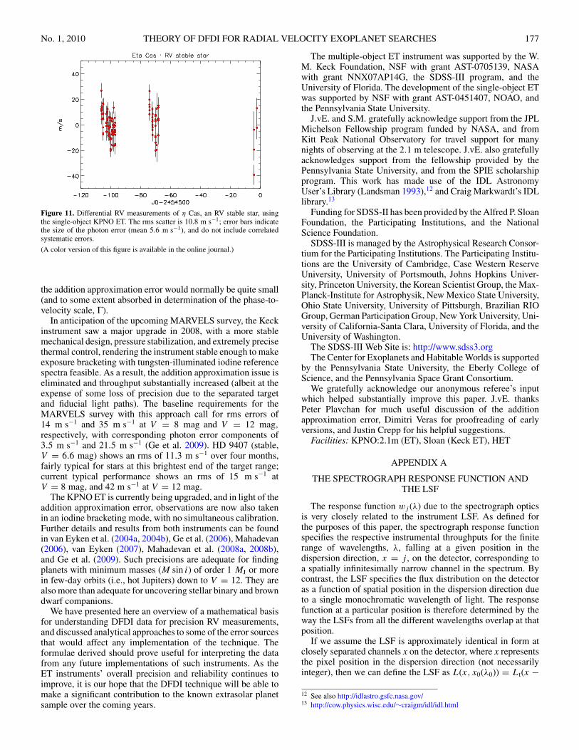
No. 1, 2010 THEORY OF DFDI FOR RADIAL VELOCITY EXOPLANET SEARCHES 177
Figure 11. Differential RV measurements of η Cas, an RV stable star, usingthe single-object KPNO ET. The rms scatter is 10.8 m s−1; error bars indicatethe size of the photon error (mean 5.6 m s−1), and do not include correlatedsystematic errors.
(A color version of this figure is available in the online journal.)
the addition approximation error would normally be quite small(and to some extent absorbed in determination of the phase-to-velocity scale, Γ).
In anticipation of the upcoming MARVELS survey, the Keckinstrument saw a major upgrade in 2008, with a more stablemechanical design, pressure stabilization, and extremely precisethermal control, rendering the instrument stable enough to makeexposure bracketing with tungsten-illuminated iodine referencespectra feasible. As a result, the addition approximation issue iseliminated and throughput substantially increased (albeit at theexpense of some loss of precision due to the separated targetand fiducial light paths). The baseline requirements for theMARVELS survey with this approach call for rms errors of14 m s−1 and 35 m s−1 at V = 8 mag and V = 12 mag,respectively, with corresponding photon error components of3.5 m s−1 and 21.5 m s−1 (Ge et al. 2009). HD 9407 (stable,V = 6.6 mag) shows an rms of 11.3 m s−1 over four months,fairly typical for stars at this brightest end of the target range;current typical performance shows an rms of 15 m s−1 atV = 8 mag, and 42 m s−1 at V = 12 mag.
The KPNO ET is currently being upgraded, and in light of theaddition approximation error, observations are now also takenin an iodine bracketing mode, with no simultaneous calibration.Further details and results from both instruments can be foundin van Eyken et al. (2004a, 2004b), Ge et al. (2006), Mahadevan(2006), van Eyken (2007), Mahadevan et al. (2008a, 2008b),and Ge et al. (2009). Such precisions are adequate for findingplanets with minimum masses (M sin i) of order 1 MJ or morein few-day orbits (i.e., hot Jupiters) down to V = 12. They arealso more than adequate for uncovering stellar binary and browndwarf companions.
We have presented here an overview of a mathematical basisfor understanding DFDI data for precision RV measurements,and discussed analytical approaches to some of the error sourcesthat would affect any implementation of the technique. Theformulae derived should prove useful for interpreting the datafrom any future implementations of such instruments. As theET instruments’ overall precision and reliability continues toimprove, it is our hope that the DFDI technique will be able tomake a significant contribution to the known extrasolar planetsample over the coming years.
The multiple-object ET instrument was supported by the W.M. Keck Foundation, NSF with grant AST-0705139, NASAwith grant NNX07AP14G, the SDSS-III program, and theUniversity of Florida. The development of the single-object ETwas supported by NSF with grant AST-0451407, NOAO, andthe Pennsylvania State University.
J.vE. and S.M. gratefully acknowledge support from the JPLMichelson Fellowship program funded by NASA, and fromKitt Peak National Observatory for travel support for manynights of observing at the 2.1 m telescope. J.vE. also gratefullyacknowledges support from the fellowship provided by thePennsylvania State University, and from the SPIE scholarshipprogram. This work has made use of the IDL AstronomyUser’s Library (Landsman 1993),12 and Craig Markwardt’s IDLlibrary.13
Funding for SDSS-II has been provided by the Alfred P. SloanFoundation, the Participating Institutions, and the NationalScience Foundation.
SDSS-III is managed by the Astrophysical Research Consor-tium for the Participating Institutions. The Participating Institu-tions are the University of Cambridge, Case Western ReserveUniversity, University of Portsmouth, Johns Hopkins Univer-sity, Princeton University, the Korean Scientist Group, the Max-Planck-Institute for Astrophysik, New Mexico State University,Ohio State University, University of Pittsburgh, Brazilian RIOGroup, German Participation Group, New York University, Uni-versity of California-Santa Clara, University of Florida, and theUniversity of Washington.
The SDSS-III Web Site is: http://www.sdss3.orgThe Center for Exoplanets and Habitable Worlds is supported
by the Pennsylvania State University, the Eberly College ofScience, and the Pennsylvania Space Grant Consortium.
We gratefully acknowledge our anonymous referee’s inputwhich helped substantially improve this paper. J.vE. thanksPeter Plavchan for much useful discussion of the additionapproximation error, Dimitri Veras for proofreading of earlyversions, and Justin Crepp for his helpful suggestions.
Facilities: KPNO:2.1m (ET), Sloan (Keck ET), HET
APPENDIX A
THE SPECTROGRAPH RESPONSE FUNCTION ANDTHE LSF
The response function wj (λ) due to the spectrograph opticsis very closely related to the instrument LSF. As defined forthe purposes of this paper, the spectrograph response functionspecifies the respective instrumental throughputs for the finiterange of wavelengths, λ, falling at a given position in thedispersion direction, x = j , on the detector, corresponding toa spatially infinitesimally narrow channel in the spectrum. Bycontrast, the LSF specifies the flux distribution on the detectoras a function of spatial position in the dispersion direction dueto a single monochromatic wavelength of light. The responsefunction at a particular position is therefore determined by theway the LSFs from all the different wavelengths overlap at thatposition.
If we assume the LSF is approximately identical in form atclosely separated channels x on the detector, where x representsthe pixel position in the dispersion direction (not necessarilyinteger), then we can define the LSF as L(x, x0(λ0)) = Lt(x −12 See also http://idlastro.gsfc.nasa.gov/13 http://cow.physics.wisc.edu/∼craigm/idl/idl.html
178 VAN EYKEN, GE, & MAHADEVAN Vol. 189
x0(λ0)) where L represents the normalized envelope of fluxspread across pixels x on the detector due to monochromaticlight of wavelength λ0, centered at position x0. L is simply ashifted version of Lt(x), which represents a template of the LSFcentered at x = 0. In general, x(λ) represents the wavelengthcalibration mapping wavelength to detector position.
The response function at an infinitesimally wide position onthe detector, w, is given by writing the contribution from eachoverlapping LSF at that position. The contribution from wave-length λ0 at position x1 is given by w(λ0, x1) = L(x1, x0(λ0)) =Lt(x1 − x0(λ0)). Therefore, as a continuous function of generalwavelength λ, we can write the response function at position x1as
w(λ, x1) = Lt(x1 − x(λ)). (A1)
We see that this is really just the LSF reversed (since the x termis now negative).
We can now extend this to the total contribution across anentire pixel at position x = j where j is now an integerrepresenting pixel number. Let tj (x ′) represent the pixel re-sponse function, describing the normalized throughput of thepixel across its width as a function of x ′. Then we can writew(λ, x ′)tj (x ′) dx ′ = Lt(x ′ − x(λ))tj (x ′) dx ′. Summing over allx ′, we have the full response function Wj for pixel column j,given by
Wj (λ) =∫
Lt(x′ − x(λ))tj (x ′) dx ′, (A2)
i.e., essentially a convolution of the response function with thepixel response function. To the extent that the width of the pixelis narrow compared to the LSF (i.e., that the image is welloversampled), then to a reasonable approximation, tj is close toa delta function, W ≈ w, and the instrument response functionat position x is approximately just the reversed LSF. Analogousarguments can be followed in wavenumber (κ) space instead ofwavelength space, simply replacing λ with κ to obtain the sameexactly the same results as a function of κ .
APPENDIX B
FRINGE FORMATION: AN ALTERNATIVE VIEWPOINT
We can view the formation of the fringes as given byEquation (8) in another way. Beginning again with Equation (1)for the flux at a given channel, j, as a function of delay d, andagain substituting Q, we can write
Ij (d) =∫
Q(κ) �{1 + e−i2πκd} dκ
=∫
P (κ)wj (κ)[1 + cos(2πκd)]dκ, (B1)
where again the spectrum within the channel is given byQ(κ) = P (κ)wj (κ), with P (κ) being the full spectrum enteringthe instrument, and wj (κ) being the spectrograph responsefunction for channel j.
If we assume that the spectrograph response function is uni-form across the whole spectrum (i.e., for all j), then we canexpress it as a wavenumber-shifted version of a global “tem-plate” spectrograph response function, wt (which is centered atκ = 0), shifted so that its center is at the central wavenumber ofthe channel in question, κj . From Appendix A, we know that thespectrograph response function is just the reverse of the LSF, sowe can write
wj = wt(κ − κj ) = Lt(κj − κ), (B2)
where Lt represents a global template LSF, also centered atκ = 0. If we furthermore define T (κ, d) ≡ 1 + cos(2πκd), wecan therefore rewrite Equation (B1) as
Ij (d) =∫
P (κ)T (κ, d)Lt(κj − κ)dκ. (B3)
T can be thought of as the interferometer transmission function,equivalent to the interferogram that would be obtained for purewhite light and an infinite resolution spectrograph (exactly as inEquation (12)). Equation (B3) can be identified as a convolutionover the variable κ:
Ij (d, κj ) = [P (κ) T (κ, d)] ⊗ Lt(κ), (B4)
where the convolution is evaluated at wavenumber κj .In other words, we have simply the input spectrum multiplied
with the interferometer transmission function, and then con-volved with the LSF due to the spectrograph. Thinking in twodimensions, to match the wide-slit format of the actual ET spec-tra, we can replace the LSF with its two-dimensional equivalent,the instrument point spread function (PSF). Exactly the sameresults can be derived in frequency space, simply by substitutingfrequency ν for κ and time delay τ for d.
This way of looking at fringe formation is the approach usedby Erskine (2003) and followed by Mahadevan (2006), and canconveniently be employed to quickly produce simulated DFDIspectra (although with the caveat that it assumes a uniform LSF,which in practice is unlikely to be very realistic).
APPENDIX C
DIVISION-OF-MEANS APPROXIMATION
In Section 3.2, we make an approximation regarding the mag-nitude of velocity errors resulting from a contaminant spectrum,where we state that the error in velocity is approximately equalto the flux ratio of the contaminant to the true source spectrummultiplied by the velocity difference between the two spectra(Equation (56)). Namely, we assume that 〈Fc/Fs〉 ≈ 〈Fc〉/〈Fs〉(we will use 〈· · ·〉 to represent the mean here for notational con-venience). The same is assumed several times in the same section(Equations (57) and (59)). This approximation holds true pro-vided that the fractional variation in the power spectrum in thedenominator with wavelength is predominantly relatively small.We also make the same approximation regarding the divisionof mean visibilities in Sections 3.3.2 and 3.3.3 (Equations (60)and (64)). Here we show the validity of this approximation.
Consider two arbitrary functions A(x) and B(x), which havefractionally relatively small variations about their means so thatwe can define two corresponding functions, a(x) and b(x) suchthat
A(x) ≡ 〈A〉(1 + a(x)); B(x) ≡ 〈B〉(1 + b(x)), (C1)
where a, b 1 for all x. Using the binomial expansion, we canwrite⟨
A
B
⟩=
⟨ 〈A〉(1 + a)
〈B〉(1 + b)
⟩= 〈A〉
〈B〉⟨
1 + a
1 + b
⟩= 〈A〉
〈B〉 〈(1 + a)(1 − b + b2 − b3 + · · ·)〉
= 〈A〉〈B〉 〈1 − b + b2 − b3 + · · · + a − ab + ab2 − ab3 + · · ·〉
≈ 〈A〉〈B〉 [1 + 〈b2〉 − 〈ab〉], (C2)

No. 1, 2010 THEORY OF DFDI FOR RADIAL VELOCITY EXOPLANET SEARCHES 179
where we have neglected terms of order b3 and ab2 and smaller,and where we can also drop the terms 〈a〉 and 〈b〉, which mustequal zero according to the definitions of a and b.
In general, 〈ab〉 → 0 if the functions a and b (and hence Aand B) are uncorrelated. In the limit where the two functionsare completely correlated (i.e., identical), then 〈ab〉 → 〈b2〉,and the 〈ab〉 and 〈b2〉 terms cancel, so that 〈A/B〉 → 〈A〉/〈B〉.In the cases we are interested in, it is generally unlikely that〈ab〉 0 (anticorrelation), or that 〈ab〉 � 〈b2〉. Therefore, wecan reasonably take 〈b2〉 as an estimate of the fractional errorin the division approximation. Conveniently, from the definitionof b, 〈b2〉 turns out to be equal to the square of the normalizedstandard deviation, σB , of the function B:
〈b2〉 = 〈(B − 〈B〉)2〉〈B〉2
=(
σB
〈B〉)2
. (C3)
Hence for functions with small fractional deviations fromtheir respective means, the mean of the quotient is approximatelyequal to the quotient of the means, and (σB/〈B〉)2 gives anestimate of the fractional error in the approximation.
Tests with stellar spectra show the approximation works quitewell, both at ET-like resolutions and with very high resolutionsynthetic spectra. Taking as an example R ∼ 5000 spectra fromthe KPNO ET of 36 UMa (F8V) and τ Cet (G8V) (obtainedby binning the fringing spectra along the slit direction), we findστCet/〈FτCet〉 = 0.25, giving an estimated error of 6% due to theapproximation. In practice, we find the ratio of 〈F36UMa〉/〈FτCet〉to 〈F36UMa/FτCet〉 to be 0.980, i.e., a 2% difference. For anemission spectrum in the denominator, such as ThAr, theapproximation will not hold well as there are significant regionsof near-zero flux. However, it is unlikely that one would beinterested in considering some contaminant spectrum against aprimary emission spectrum source. Conceivably one might beinterested in considering the effects of contamination from anemission source—e.g., from stray fluorescent lighting leakage,sky emission, or leakage from an reference lamp, but in thiscase the emission spectrum would be in the numerator: a stellarspectrum will always be the function in the denominator, and sothe approximation should still hold.
The second case where the approximation is employed is inconsidering visibility ratios, as in estimating the velocity errordue to the reference whirl addition approximation, or estimatingthe effect of residual interferometer comb (Equations (60) and(64)). In both cases here the function in the denominatoris absolute visibility as a function of wavelength, α(λ), forreference-multiplied stellar data (since the comb and cross-talk terms both appear in the formula for the combined star/reference data, Equation (22)). Taking KPNO spectra as anexample, the normalized variance of the combined star/iodinedata tends to be around (σα/〈α〉)2 ≈ 0.32, in other words givingan estimated error in the division approximation of around 30%for both comb and cross-talk error sources—not as precise asthe approximation for contaminating spectra, but still useful foran order-of-magnitude error. In neither of these cases do weexpect any correlation between the data visibility function inthe denominator and the comb or cross-talk visibility functionin the numerator, so the 〈ab〉 term should be small.
Where there is concern over the assumptions made above(e.g., where the normalized variance of the denominator,(σB /〈B〉)2 is not small—which would, for example, be the casewere the denominator to represent visibilities of a pure star spec-trum, where the visibility distribution peaks at very low values),
then the approximation derived here is not appropriate, and in-stead it is necessary to calculate 〈Fc/Fs〉 directly. Often this is infact entirely practical; however the approximation can generallybe used to give a very quick and convenient first-order estimateof contamination errors.
REFERENCES
Armitage, P. J. 2007, ApJ, 665, 1381Baranne, A., et al. 1996, A&AS, 119, 373Barker, L. M., & Hollenbach, R. E. 1972, J. Appl. Phys., 43, 4669Barker, L. M., & Schuler, K. W. 1974, J. Appl. Phys., 45, 3692Beckers, J. M., & Brown, T. M. 1978, in Proc. JOSO Workshop, Future Solar
Optical Observations Needs and Constraints, ed. G. Godoli, G. Noci, & A.Righini (Firenze: Baccini e Chiappi), 189
Behr, B. B., Hajian, A. R., Cenko, A. T., Murison, M., McMillan, R. S., Hindsley,R., & Meade, J. 2009, ApJ, 705, 543
Butler, R. P., Marcy, G. W., Williams, E., McCarthy, C., Dosanjh, P., & Vogt, S.S. 1996, PASP, 108, 500
Campbell, B., & Walker, G. A. H. 1979, PASP, 91, 540Connes, P. 1985, Ap&SS, 110, 211da Silva, R., et al. 2006, A&A, 446, 717Douglas, N. G. 1997, PASP, 109, 151Edelstein, J., Erskine, D. J., Lloyd, J., Herter, T., Marckwordt, M., & Feuerstein,
M. 2006, Proc. SPIE, 6269, 62691EEdser, E., & Butler, C. P. 1898, Philos. Mag., 46, 207Erskine, D. J. 2003, PASP, 115, 255Erskine, D. J., & Edelstein, J. 2004, Proc. SPIE, 5492, 190Erskine, D. J., Edelstein, J., Feuerstein, W. M., & Welsh, B. 2003, ApJ, 592,
L103Erskine, D. J., & Ge, J. 2000, in ASP Conf. Ser. 195, Imaging the Universe in
Three Dimensions, ed. W. van Breugel & J. Bland-Hawthorn (San Francisco,CA: ASP), 501
Fischer, D. A., & Valenti, J. 2005, ApJ, 622, 1102Forrest, A. K., & Ring, J. 1978, in Proc. 4th International Colloquium
on Astrophysics, High Resolution Spectrometry, ed. M. Hack (Trieste:Osservatorio astronomico di Trieste), 462
Frandsen, S., Douglas, N. G., & Butcher, H. R. 1993, A&A, 279, 310Ge, J. 2002, ApJ, 571, L165Ge, J., Eisenstein, D., & Gaudi, B. S. 2009, Astro2010 Astronomy and
Astrophysics Decadal Survey Science White Paper, 86 (arXiv:0903.0181)Ge, J., Erskine, D. J., & Rushford, M. 2002, PASP, 114, 1016Ge, J., Mahadevan, S., van Eyken, J., Dewitt, C., & Shaklan, S. 2003a, in ASP
Conf. Ser. 294, Scientific Frontiers in Research on Extrasolar Planets, ed. D.Deming, S. Seager (San Francisco, CA: ASP), 573
Ge, J., van Eyken, J. C., Mahadevan, S., DeWitt, C., Ramsey, L. W., Shaklan,S. B., & Pan, X. 2003b, Proc. SPIE, 4838, 503
Ge, J., et al. 2006, ApJ, 648, 683Geake, J. E., Ring, J., & Woolf, N. J. 1959, MNRAS, 119, 616Goodman, J. W. 1985, Statistical Optics (New York: Wiley)Gorskii, S. M., & Lebedev, V. P. 1977, Izv. Krym. Astrofizika Obs., 57, 228Griffin, R., & Griffin, R. 1973, MNRAS, 162, 243Hajian, A. R., et al. 2007, ApJ, 661, 616Harlander, J., Reynolds, R. J., & Roesler, F. L. 1992, ApJ, 396, 730Harvey, J., & The GONG Instrument Team 1995, in ASP Conf. Ser. 76, GONG
1994. Helio- and Astro-Seismology from the Earth and Space, ed. R. K.Ulrich, E. J. Rhodes, & Jr., W. Dappen (San Francisco, CA: ASP), 432
Hilliard, R. L., & Shepherd, G. G. 1966, J. Opt. Soc. Am., 56, 362Jacquinot, P. 1960, Rep. Prog. Phys., 23, 267Johnson, J. A., et al. 2006, ApJ, 647, 600Kane, S. R., Collier Cameron, A., Horne, K., James, D., Lister, T. A., Pollacco,
D. L., Street, R. A., & Tsapras, Y. 2004, MNRAS, 353, 689Konacki, M., Muterspaugh, M. W., Kulkarni, S. R., & Hełminiak, K. G.
2009, ApJ, 704, 513Landsman, W. B. 1993, in ASP Conf. Ser. 52, Astronomical Data Analysis
Software and Systems II, ed. R. J. Hanisch, R. J. V. Brissenden, & J. Barnes(San Francisco, CA: ASP), 246
Lawson, P. R. 2000, in Principles of Long Baseline Stellar Interferometry, ed.P. R. Lawson (Pasadena, CA: NASA JPL), 113
Loeillet, B., et al. 2008, A&A, 479, 865Mahadevan, S. 2006, PhD thesis, Univ. of FloridaMahadevan, S., Ge, J., Fleming, S. W., Wan, X., DeWitt, C., van Eyken, J. C.,
& McDavitt, D. 2008a, PASP, 120, 1001Mahadevan, S., Ge, J., van Eyken, J. C., DeWitt, C., & Shaklan, S. B. 2003,
Proc. SPIE, 5170, 184

180 VAN EYKEN, GE, & MAHADEVAN Vol. 189
Mahadevan, S., van Eyken, J., Ge, J., DeWitt, C., Fleming, S. W., Cohen, R.,Crepp, J., & Vanden Heuvel, A. 2008b, ApJ, 678, 1505
Mayor, M., & Queloz, D. 1995, Nature, 378, 355McMillan, R. S., Moore, T. L., Perry, M. L., & Smith, P. H. 1993, ApJ, 403, 801McMillan, R. S., Moore, T. L., Perry, M. L., & Smith, P. H. 1994, Ap&SS, 212,
271Michelson, A. A. 1903, Light Waves and their Uses (Chicago, IL: Univ. of
Chicago Press)Mosser, B., Maillard, J.-P., & Bouchy, F. 2003, PASP, 115, 990Pepe, F., et al. 2005, Messenger, 120, 22Shepherd, G. G., et al. 1985, Appl. Opt., 24, 1571
Szentgyorgyi, A. H., & Furesz, G. 2007, RevMexAA Conf. Ser., 28, 129Udry, S., Fischer, D., & Queloz, D. 2007, in Protostars and Planets V, ed. B.
Reipurth, D. Jewitt, & K. Keil (Tucson, AZ: Univ. Arizona Press), 685van Eyken, J. C. 2007, PhD thesis, Univ. of Floridavan Eyken, J. C., Ge, J., Mahadevan, S., & DeWitt, C. 2004a, ApJ, 600,
L79van Eyken, J. C., Ge, J., Mahadevan, S., DeWitt, C., Friedman, J., Finnerty, P.,
Ren, D., & Zugger, M. 2004b, Proc. SPIE, 5492, 445van Eyken, J. C., Ge, J., Mahadevan, S., DeWitt, C., & Ren, D. 2003, Proc. SPIE,
5170, 250Vogt, S. S., Marcy, G. W., Butler, R. P., & Apps, K. 2000, ApJ, 536, 902