Theory of Applied Robotics

Reza N. Jazar

Theory of Applied Robotics

Kinematics, Dynamics, and Control

Second Edition

123

Prof. Reza N. JazarSchool of Aerospace, Mechanical, andManufacturing EngineeringRMIT UniversityMelbourne, VictoriaAustraliareza.reza.jazar@rmit.edu.au

ISBN 978-1-4419-1749-2 e-ISBN 978-1-4419-1750-8DOI 10.1007/978-1-4419-1750-8Springer New York Dordrecht Heidelberg London

Library of Congress Control Number:

c© Springer Science+Business Media, LLC 20102006,

201092 0336

All rights reserved. This work may not be translated or copied in whole or in part without the writtenpermission of the publisher (Springer Science+Business Media, LLC, 233 Spring Street, New York,NY 10013, USA), except for brief excerpts in connection with reviews or scholarly analysis. Use inconnection with any form of information storage and retrieval, electronic adaptation, computersoftware, or by similar or dissimilar methodology now known or hereafter developed is forbidden.The use in this publication of trade names, trademarks, service marks, and similar terms, even ifthey are not identified as such, is not to be taken as an expression of opinion as to whether or notthey are subject to proprietary rights.

Cover illustration c©Konstantin Inozemtsev

Printed on acid-free paper

Springer is part of Springer Science+Business Media (www.springer.com)

Dedicated to my wife,Mojgan

and our children,Vazanand

Kavosh.

I am Cyrus, king of the world, great king, mighty king,king of Babylon, king of Sumer and Akkad, king of the four quarters.

I ordered to write books, many books, books to teach my people,I ordered to make schools, many schools, to educate my people.

Marduk, the lord of the gods, said burning books is the greatest sin.I, Cyrus, and my people, and my army will protect books and schools.They will fight whoever burns books and burns schools, the great sin.

Cyrus the great

Preface to the Second Edition

The second edition of this book would not have been possible without the comments and suggestions from my students, especially those at Columbia University. Many of the new topics introduced here are a direct result of student feedback that helped me refine and clarify the material.

My intention when writing this book was to develop material that I would have liked to had available as a student. Hopefully, I have succeeded in developing a reference that covers all aspects of robotics with sufficient detail and explanation.

The first edition of this book was published in 2007 and soon after its publication it became a very popular reference in the field of robotics. I wish to thank the many students and instructors who have used the book or referenced it. Your questions, comments and suggestions have helped me create the second edition.

Preface

This book is designed to serve as a text for engineering students. Itintroduces the fundamental knowledge used in robotics. This knowledgecan be utilized to develop computer programs for analyzing the kinematics,dynamics, and control of robotic systems.The subject of robotics may appear overdosed by the number of available

texts because the field has been growing rapidly since 1970. However, thetopic remains alive with modern developments, which are closely related tothe classical material. It is evident that no single text can cover the vastscope of classical and modern materials in robotics. Thus the demand fornew books arises because the field continues to progress. Another factoris the trend toward analytical unification of kinematics, dynamics, andcontrol.Classical kinematics and dynamics of robots has its roots in the work of

great scientists of the past four centuries who established the methodologyand understanding of the behavior of dynamic systems. The developmentof dynamic science, since the beginning of the twentieth century, has movedtoward analysis of controllable man-made systems. Therefore, merging thekinematics and dynamics with control theory is the expected developmentfor robotic analysis.The other important development is the fast growing capability of ac-

curate and rapid numerical calculations, along with intelligent computerprogramming.

Level of the BookThis book has evolved from nearly a decade of research in nonlinear

dynamic systems, and teaching undergraduate-graduate level courses inrobotics. It is addressed primarily to the last year of undergraduate studyand the first year graduate student in engineering. Hence, it is an interme-diate textbook. This book can even be the first exposure to topics in spa-tial kinematics and dynamics of mechanical systems. Therefore, it providesboth fundamental and advanced topics on the kinematics and dynamics ofrobots. The whole book can be covered in two successive courses however,it is possible to jump over some sections and cover the book in one course.The students are required to know the fundamentals of kinematics anddynamics, as well as a basic knowledge of numerical methods.

The contents of the book have been kept at a fairly theoretical-practicallevel. Many concepts are deeply explained and their use emphasized, andmost of the related theory and formal proofs have been explained. Through-out the book, a strong emphasis is put on the physical meaning of the con-cepts introduced. Topics that have been selected are of high interest in thefield. An attempt has been made to expose the students to a broad rangeof topics and approaches.

Organization of the BookThe text is organized so it can be used for teaching or for self-study.

Chapter 1 “Introduction,” contains general preliminaries with a brief reviewof the historical development and classification of robots.Part I “Kinematics,” presents the forward and inverse kinematics of

robots. Kinematics analysis refers to position, velocity, and accelerationanalysis of robots in both joint and base coordinate spaces. It establisheskinematic relations among the end-effecter and the joint variables. Themethod of Denavit-Hartenberg for representing body coordinate frames isintroduced and utilized for forward kinematics analysis. The concept ofmodular treatment of robots is well covered to show how we may combinesimple links to make the forward kinematics of a complex robot. For inversekinematics analysis, the idea of decoupling, the inverse matrix method, andthe iterative technique are introduced. It is shown that the presence of aspherical wrist is what we need to apply analytic methods in inverse kine-matics.Part II “Dynamics,” presents a detailed discussion of robot dynamics.

An attempt is made to review the basic approaches and demonstrate howthese can be adapted for the active displacement framework utilized forrobot kinematics in the earlier chapters. The concepts of the recursiveNewton-Euler dynamics, Lagrangian function, manipulator inertia matrix,and generalized forces are introduced and applied for derivation of dynamicequations of motion.Part III “Control,” presents the floating time technique for time-optimal

control of robots. The outcome of the technique is applied for an open-loop control algorithm. Then, a computed-torque method is introduced, inwhich a combination of feedforward and feedback signals are utilized torender the system error dynamics.

Method of PresentationThe structure of presentation is in a "fact-reason-application" fashion.

The "fact" is the main subject we introduce in each section. Then thereason is given as a "proof." Finally the application of the fact is examinedin some "examples." The "examples" are a very important part of the bookbecause they show how to implement the knowledge introduced in "facts."They also cover some other facts that are needed to expand the subject.

Prefacexii

PrerequisitesSince the book is written for senior undergraduate and first-year graduate

level students of engineering, the assumption is that users are familiar withmatrix algebra as well as basic feedback control. Prerequisites for readersof this book consist of the fundamentals of kinematics, dynamics, vectoranalysis, and matrix theory. These basics are usually taught in the firstthree undergraduate years.

Unit SystemThe system of units adopted in this book is, unless otherwise stated,

the international system of units (SI). The units of degree (deg) or radian( rad) are utilized for variables representing angular quantities.

Symbols

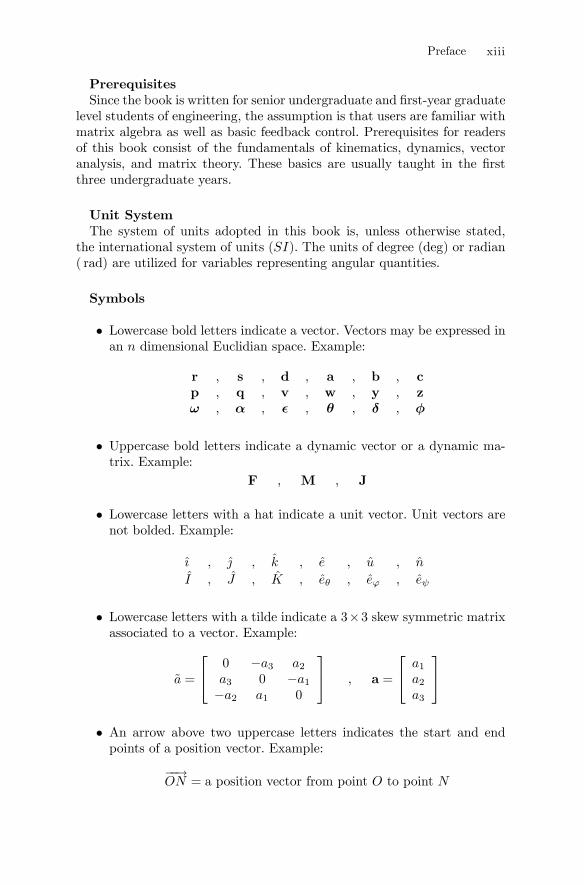
• Lowercase bold letters indicate a vector. Vectors may be expressed inan n dimensional Euclidian space. Example:

r , s , d , a , b , cp , q , v , w , y , zω , α , ² , θ , δ , φ

• Uppercase bold letters indicate a dynamic vector or a dynamic ma-trix. Example:

F , M , J

• Lowercase letters with a hat indicate a unit vector. Unit vectors arenot bolded. Example:

ı , j , k , e , u , n

I , J , K , eθ , eϕ , eψ

• Lowercase letters with a tilde indicate a 3×3 skew symmetric matrixassociated to a vector. Example:

a =

⎡⎣ 0 −a3 a2a3 0 −a1−a2 a1 0

⎤⎦ , a =

⎡⎣ a1a2a3

⎤⎦• An arrow above two uppercase letters indicates the start and endpoints of a position vector. Example:

−−→ON = a position vector from point O to point N

Preface xiii

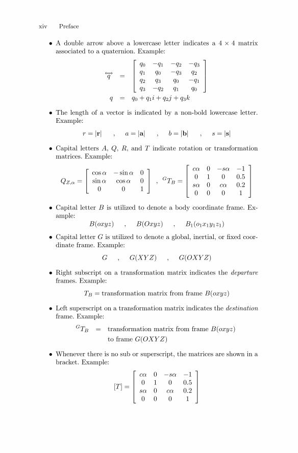
• A double arrow above a lowercase letter indicates a 4 × 4 matrixassociated to a quaternion. Example:

←→q =

⎡⎢⎢⎣q0 −q1 −q2 −q3q1 q0 −q3 q2q2 q3 q0 −q1q3 −q2 q1 q0

⎤⎥⎥⎦q = q0 + q1i+ q2j + q3k

• The length of a vector is indicated by a non-bold lowercase letter.Example:

r = |r| , a = |a| , b = |b| , s = |s|

• Capital letters A, Q, R, and T indicate rotation or transformationmatrices. Example:

QZ,α =

⎡⎣ cosα − sinα 0sinα cosα 00 0 1

⎤⎦ , GTB =

⎡⎢⎢⎣cα 0 −sα −10 1 0 0.5sα 0 cα 0.20 0 0 1

⎤⎥⎥⎦• Capital letter B is utilized to denote a body coordinate frame. Ex-ample:

B(oxyz) , B(Oxyz) , B1(o1x1y1z1)

• Capital letter G is utilized to denote a global, inertial, or fixed coor-dinate frame. Example:

G , G(XY Z) , G(OXY Z)

• Right subscript on a transformation matrix indicates the departureframes. Example:

TB = transformation matrix from frame B(oxyz)

• Left superscript on a transformation matrix indicates the destinationframe. Example:

GTB = transformation matrix from frame B(oxyz)

to frame G(OXY Z)

• Whenever there is no sub or superscript, the matrices are shown in abracket. Example:

[T ] =

⎡⎢⎢⎣cα 0 −sα −10 1 0 0.5sα 0 cα 0.20 0 0 1

⎤⎥⎥⎦

Prefacevix

• Left superscript on a vector denotes the frame in which the vectoris expressed. That superscript indicates the frame that the vectorbelongs to; so the vector is expressed using the unit vectors of thatframe. Example:

Gr = position vector expressed in frame G(OXY Z)

• Right subscript on a vector denotes the tip point that the vector isreferred to. Example:

GrP = position vector of point P

expressed in coordinate frame G(OXY Z)

• Left subscript on a vector indicates the frame that the angular vectoris measured with respect to. Example:

GBvP = velocity vector of point P in coordinate frame B(oxyz)

expressed in the global coordinate frame G(OXY Z)

We drop the left subscript if it is the same as the left superscript.Example:

BBvP ≡ BvP

• Right subscript on an angular velocity vector indicates the frame thatthe angular vector is referred to. Example:

ωB = angular velocity of the body coordinate frame B(oxyz)

• Left subscript on an angular velocity vector indicates the frame thatthe angular vector is measured with respect to. Example:

GωB = angular velocity of the body coordinate frame B(oxyz)

with respect to the global coordinate frame G(OXY Z)

• Left superscript on an angular velocity vector denotes the frame inwhich the angular velocity is expressed. Example:

B2

G ωB1 = angular velocity of the body coordinate frame B1with respect to the global coordinate frame G,

and expressed in body coordinate frame B2

Whenever the left subscript and superscript of an angular velocityare the same, we usually drop the left superscript. Example:

GωB ≡ GGωB

Preface vx

• If the right subscript on a force vector is a number, it indicates thenumber of coordinate frame in a serial robot. Coordinate frame Bi isset up at joint i+ 1. Example:

Fi = force vector at joint i+ 1

measured at the origin of Bi(oxyz)

At joint i there is always an action force Fi, that link (i) applies onlink (i+1), and a reaction force −Fi, that link (i+1) applies on link(i). On link (i) there is always an action force Fi−1 coming from link(i − 1), and a reaction force −Fi coming from link (i + 1). Actionforce is called driving force, and reaction force is called driven force.

• If the right subscript on a moment vector is a number, it indicatesthe number of coordinate frames in a serial robot. Coordinate frameBi is set up at joint i+ 1. Example:

Mi = moment vector at joint i+ 1

measured at the origin of Bi(oxyz)

At joint i there is always an action momentMi, that link (i) applieson link (i+1), and a reaction moment −Mi, that link (i+1) applieson link (i). On link (i) there is always an action momentMi−1 comingfrom link (i−1), and a reaction moment −Mi coming from link (i+1).Action moment is called driving moment, and reaction moment iscalled driven moment.

• Left superscript on derivative operators indicates the frame in whichthe derivative of a variable is taken. Example:

Gd

dtx ,

Gd

dtBrP ,

Bd

dtGBrP

If the variable is a vector function, and also the frame in which thevector is defined is the same as the frame in which a time derivativeis taken, we may use the following short notation,

Gd

dtGrP =

GrP ,Bd

dtBo rP =

Bo rP

and write equations simpler. Example:

Gv =Gd

dtGr(t) = Gr

• If followed by angles, lowercase c and s denote cos and sin functionsin mathematical equations. Example:

cα = cosα , sϕ = sinϕ

i Prefacevx

• Capital bold letter I indicates a unit matrix, which, depending onthe dimension of the matrix equation, could be a 3 × 3 or a 4 × 4unit matrix. I3 or I4 are also being used to clarify the dimension ofI. Example:

I = I3 =

⎡⎣ 1 0 00 1 00 0 1

⎤⎦• An asterisk F indicates a more advanced subject or example that isnot designed for undergraduate teaching and can be dropped in thefirst reading.

• Two parallel joint axes are indicated by a parallel sign, (k).

• Two orthogonal joint axes are indicated by an orthogonal sign, (`).Two orthogonal joint axes are intersecting at a right angle.

• Two perpendicular joint axes are indicated by a perpendicular sign,(⊥). Two perpendicular joint axes are at a right angle with respectto their common normal.

Preface ivx i

Contents

1 Introduction 11.1 Historical Development . . . . . . . . . . . . . . . . . . . . 21.2 Robot Components . . . . . . . . . . . . . . . . . . . . . . . 3

1.2.1 Link . . . . . . . . . . . . . . . . . . . . . . . . . . . 31.2.2 Joint . . . . . . . . . . . . . . . . . . . . . . . . . . 31.2.3 Manipulator . . . . . . . . . . . . . . . . . . . . . . . 51.2.4 Wrist . . . . . . . . . . . . . . . . . . . . . . . . . . 51.2.5 End-effector . . . . . . . . . . . . . . . . . . . . . . . 61.2.6 Actuators . . . . . . . . . . . . . . . . . . . . . . . . 71.2.7 Sensors . . . . . . . . . . . . . . . . . . . . . . . . . 71.2.8 Controller . . . . . . . . . . . . . . . . . . . . . . . . 7

1.3 Robot Classifications . . . . . . . . . . . . . . . . . . . . . . 81.3.1 Geometry . . . . . . . . . . . . . . . . . . . . . . . . 81.3.2 Workspace . . . . . . . . . . . . . . . . . . . . . . . 131.3.3 Actuation . . . . . . . . . . . . . . . . . . . . . . . 131.3.4 Control . . . . . . . . . . . . . . . . . . . . . . . . 131.3.5 Application . . . . . . . . . . . . . . . . . . . . . . 14

1.4 Introduction to Robot’s Kinematics, Dynamics, and Control 151.4.1 F Triad . . . . . . . . . . . . . . . . . . . . . . . . . 161.4.2 Unit Vectors . . . . . . . . . . . . . . . . . . . . . . 161.4.3 Reference Frame and Coordinate System . . . . . . 171.4.4 Vector Function . . . . . . . . . . . . . . . . . . . . 20

1.5 Problems of Robot Dynamics . . . . . . . . . . . . . . . . . 201.6 Preview of Covered Topics . . . . . . . . . . . . . . . . . . . 221.7 Robots as Multi-disciplinary Machines . . . . . . . . . . . . 231.8 Summary . . . . . . . . . . . . . . . . . . . . . . . . . . . . 24Exercises . . . . . . . . . . . . . . . . . . . . . . . . . . . . . . . 25

I Kinematics 29

2 Rotation Kinematics 332.1 Rotation About Global Cartesian Axes . . . . . . . . . . . . 332.2 Successive Rotation About Global Cartesian Axes . . . . . 402.3 Global Roll-Pitch-Yaw Angles . . . . . . . . . . . . . . . . . 442.4 Rotation About Local Cartesian Axes . . . . . . . . . . . . 462.5 Successive Rotation About Local Cartesian Axes . . . . . . 50

2.6 Euler Angles . . . . . . . . . . . . . . . . . . . . . . . . . . 522.7 Local Roll-Pitch-Yaw Angles . . . . . . . . . . . . . . . . . 622.8 Local Axes Versus Global Axes Rotation . . . . . . . . . . . 632.9 General Transformation . . . . . . . . . . . . . . . . . . . . 652.10 Active and Passive Transformation . . . . . . . . . . . . . . 732.11 Summary . . . . . . . . . . . . . . . . . . . . . . . . . . . . 772.12 Key Symbols . . . . . . . . . . . . . . . . . . . . . . . . . . 79Exercises . . . . . . . . . . . . . . . . . . . . . . . . . . . . . . . 81

3 Orientation Kinematics 913.1 Axis-angle Rotation . . . . . . . . . . . . . . . . . . . . . . 913.2 F Euler Parameters . . . . . . . . . . . . . . . . . . . . . . 1023.3 F Determination of Euler Parameters . . . . . . . . . . . . 1103.4 F Quaternions . . . . . . . . . . . . . . . . . . . . . . . . . 1123.5 F Spinors and Rotators . . . . . . . . . . . . . . . . . . . . 1163.6 F Problems in Representing Rotations . . . . . . . . . . . . 118

3.6.1 F Rotation matrix . . . . . . . . . . . . . . . . . . . 1193.6.2 F Angle-axis . . . . . . . . . . . . . . . . . . . . . . 1203.6.3 F Euler angles . . . . . . . . . . . . . . . . . . . . . 1213.6.4 F Quaternion . . . . . . . . . . . . . . . . . . . . . 1223.6.5 F Euler parameters . . . . . . . . . . . . . . . . . . 124

3.7 F Composition and Decomposition of Rotations . . . . . . 1263.8 Summary . . . . . . . . . . . . . . . . . . . . . . . . . . . . 1333.9 Key Symbols . . . . . . . . . . . . . . . . . . . . . . . . . . 135Exercises . . . . . . . . . . . . . . . . . . . . . . . . . . . . . . . 137

4 Motion Kinematics 1494.1 Rigid Body Motion . . . . . . . . . . . . . . . . . . . . . . . 1494.2 Homogeneous Transformation . . . . . . . . . . . . . . . . . 1544.3 Inverse Homogeneous Transformation . . . . . . . . . . . . 1624.4 Compound Homogeneous Transformation . . . . . . . . . . 1684.5 F Screw Coordinates . . . . . . . . . . . . . . . . . . . . . 1784.6 F Inverse Screw . . . . . . . . . . . . . . . . . . . . . . . . 1954.7 F Compound Screw Transformation . . . . . . . . . . . . . 1984.8 F The Plücker Line Coordinate . . . . . . . . . . . . . . . . 2014.9 F The Geometry of Plane and Line . . . . . . . . . . . . . 208

4.9.1 F Moment . . . . . . . . . . . . . . . . . . . . . . . 2084.9.2 F Angle and Distance . . . . . . . . . . . . . . . . . 2094.9.3 F Plane and Line . . . . . . . . . . . . . . . . . . . 209

4.10 F Screw and Plücker Coordinate . . . . . . . . . . . . . . . 2144.11 Summary . . . . . . . . . . . . . . . . . . . . . . . . . . . . 2174.12 Key Symbols . . . . . . . . . . . . . . . . . . . . . . . . . . 219Exercises . . . . . . . . . . . . . . . . . . . . . . . . . . . . . . . 221

Contentsxx

5.1 Denavit-Hartenberg Notation . . . . . . . . . . . . . . . . . 2335.2 Transformation Between Two Adjacent Coordinate Frames 2425.3 Forward Position Kinematics of Robots . . . . . . . . . . . 2595.4 Spherical Wrist . . . . . . . . . . . . . . . . . . . . . . . . . 2705.5 Assembling Kinematics . . . . . . . . . . . . . . . . . . . . . 2805.6 F Coordinate Transformation Using Screws . . . . . . . . . 2925.7 F Non Denavit-Hartenberg Methods . . . . . . . . . . . . . 2975.8 Summary . . . . . . . . . . . . . . . . . . . . . . . . . . . . 3055.9 Key Symbols . . . . . . . . . . . . . . . . . . . . . . . . . . 307Exercises . . . . . . . . . . . . . . . . . . . . . . . . . . . . . . . 309

6 Inverse Kinematics 3256.1 Decoupling Technique . . . . . . . . . . . . . . . . . . . . . 3256.2 Inverse Transformation Technique . . . . . . . . . . . . . . 3416.3 F Iterative Technique . . . . . . . . . . . . . . . . . . . . . 3576.4 F Comparison of the Inverse Kinematics Techniques . . . . 361

6.4.1 F Existence and Uniqueness of Solution . . . . . . . 3616.4.2 F Inverse Kinematics Techniques . . . . . . . . . . . 362

6.5 F Singular Configuration . . . . . . . . . . . . . . . . . . . 3636.6 Summary . . . . . . . . . . . . . . . . . . . . . . . . . . . . 3676.7 Key Symbols . . . . . . . . . . . . . . . . . . . . . . . . . . 369Exercises . . . . . . . . . . . . . . . . . . . . . . . . . . . . . . . 371

7 Angular Velocity 3817.1 Angular Velocity Vector and Matrix . . . . . . . . . . . . . 3817.2 F Time Derivative and Coordinate Frames . . . . . . . . . 3937.3 Rigid Body Velocity . . . . . . . . . . . . . . . . . . . . . . 4037.4 F Velocity Transformation Matrix . . . . . . . . . . . . . . 4097.5 Derivative of a Homogeneous Transformation Matrix . . . . 4177.6 Summary . . . . . . . . . . . . . . . . . . . . . . . . . . . . 4257.7 Key Symbols . . . . . . . . . . . . . . . . . . . . . . . . . . 427Exercises . . . . . . . . . . . . . . . . . . . . . . . . . . . . . . . 429

8 Velocity Kinematics 4378.1 F Rigid Link Velocity . . . . . . . . . . . . . . . . . . . . . 4378.2 Forward Velocity Kinematics . . . . . . . . . . . . . . . . . 4428.3 Jacobian Generating Vectors . . . . . . . . . . . . . . . . . 4528.4 Inverse Velocity Kinematics . . . . . . . . . . . . . . . . . . 4658.5 Summary . . . . . . . . . . . . . . . . . . . . . . . . . . . . 4738.6 Key Symbols . . . . . . . . . . . . . . . . . . . . . . . . . . 475Exercises . . . . . . . . . . . . . . . . . . . . . . . . . . . . . . . 477

9 Numerical Methods in Kinematics 4859.1 Linear Algebraic Equations . . . . . . . . . . . . . . . . . . 4859.2 Matrix Inversion . . . . . . . . . . . . . . . . . . . . . . . . 497

5 Forward Kinematics 233

Contents xxi

9.3 Nonlinear Algebraic Equations . . . . . . . . . . . . . . . . 5039.4 F Jacobian Matrix From Link Transformation Matrices . . 5109.5 Summary . . . . . . . . . . . . . . . . . . . . . . . . . . . . 5189.6 Key Symbols . . . . . . . . . . . . . . . . . . . . . . . . . . 519Exercises . . . . . . . . . . . . . . . . . . . . . . . . . . . . . . . 521

II Dynamics 525

10 Acceleration Kinematics 52910.1 Angular Acceleration Vector and Matrix . . . . . . . . . . . 52910.2 Rigid Body Acceleration . . . . . . . . . . . . . . . . . . . . 53810.3 F Acceleration Transformation Matrix . . . . . . . . . . . . 54110.4 Forward Acceleration Kinematics . . . . . . . . . . . . . . . 54910.5 Inverse Acceleration Kinematics . . . . . . . . . . . . . . . . 55210.6 F Rigid Link Recursive Acceleration . . . . . . . . . . . . . 55610.7 Summary . . . . . . . . . . . . . . . . . . . . . . . . . . . . 56710.8 Key Symbols . . . . . . . . . . . . . . . . . . . . . . . . . . 569Exercises . . . . . . . . . . . . . . . . . . . . . . . . . . . . . . . 571

11 Motion Dynamics 58111.1 Force and Moment . . . . . . . . . . . . . . . . . . . . . . . 58111.2 Rigid Body Translational Kinetics . . . . . . . . . . . . . . 58611.3 Rigid Body Rotational Kinetics . . . . . . . . . . . . . . . . 58811.4 Mass Moment of Inertia Matrix . . . . . . . . . . . . . . . . 59911.5 Lagrange’s Form of Newton’s Equations . . . . . . . . . . . 61111.6 Lagrangian Mechanics . . . . . . . . . . . . . . . . . . . . . 62011.7 Summary . . . . . . . . . . . . . . . . . . . . . . . . . . . . 62711.8 Key Symbols . . . . . . . . . . . . . . . . . . . . . . . . . . 629Exercises . . . . . . . . . . . . . . . . . . . . . . . . . . . . . . . 631

12 Robot Dynamics 64112.1 Rigid Link Newton-Euler Dynamics . . . . . . . . . . . . . 64112.2 F Recursive Newton-Euler Dynamics . . . . . . . . . . . . 66112.3 Robot Lagrange Dynamics . . . . . . . . . . . . . . . . . . . 66912.4 F Lagrange Equations and Link Transformation Matrices . 69012.5 Robot Statics . . . . . . . . . . . . . . . . . . . . . . . . . . 70012.6 Summary . . . . . . . . . . . . . . . . . . . . . . . . . . . . 70912.7 Key Symbols . . . . . . . . . . . . . . . . . . . . . . . . . . 713Exercises . . . . . . . . . . . . . . . . . . . . . . . . . . . . . . . 715

III Control 725

13 Path Planning 729

i i Contents

13.1 Cubic Path . . . . . . . . . . . . . . . . . . . . . . . . . . . 72913.2 Polynomial Path . . . . . . . . . . . . . . . . . . . . . . . . 735

xx

13.3 F Non-Polynomial Path Planning . . . . . . . . . . . . . . 74713.4 Manipulator Motion by Joint Path . . . . . . . . . . . . . . 74913.5 Cartesian Path . . . . . . . . . . . . . . . . . . . . . . . . . 75413.6 F Rotational Path . . . . . . . . . . . . . . . . . . . . . . . 75913.7 Manipulator Motion by End-Effector Path . . . . . . . . . . 76313.8 Summary . . . . . . . . . . . . . . . . . . . . . . . . . . . . 77713.9 Key Symbols . . . . . . . . . . . . . . . . . . . . . . . . . . 779Exercises . . . . . . . . . . . . . . . . . . . . . . . . . . . . . . . 781

14 F Time Optimal Control 79114.1 F Minimum Time and Bang-Bang Control . . . . . . . . . 79114.2 F Floating Time Method . . . . . . . . . . . . . . . . . . . 80114.3 F Time-Optimal Control for Robots . . . . . . . . . . . . . 81114.4 Summary . . . . . . . . . . . . . . . . . . . . . . . . . . . . 81714.5 Key Symbols . . . . . . . . . . . . . . . . . . . . . . . . . . 819Exercises . . . . . . . . . . . . . . . . . . . . . . . . . . . . . . . 821

15 Control Techniques 82715.1 Open and Closed-Loop Control . . . . . . . . . . . . . . . . 82715.2 Computed Torque Control . . . . . . . . . . . . . . . . . . . 83315.3 Linear Control Technique . . . . . . . . . . . . . . . . . . . 838

15.3.1 Proportional Control . . . . . . . . . . . . . . . . . . 83915.3.2 Integral Control . . . . . . . . . . . . . . . . . . . . 83915.3.3 Derivative Control . . . . . . . . . . . . . . . . . . . 839

15.4 Sensing and Control . . . . . . . . . . . . . . . . . . . . . . 84215.4.1 Position Sensors . . . . . . . . . . . . . . . . . . . . 84315.4.2 Speed Sensors . . . . . . . . . . . . . . . . . . . . . . 84315.4.3 Acceleration Sensors . . . . . . . . . . . . . . . . . . 844

15.5 Summary . . . . . . . . . . . . . . . . . . . . . . . . . . . . 84515.6 Key Symbols . . . . . . . . . . . . . . . . . . . . . . . . . . 847Exercises . . . . . . . . . . . . . . . . . . . . . . . . . . . . . . . 849

References 853

A Global Frame Triple Rotation 863

B Local Frame Triple Rotation 865

C Principal Central Screws Triple Combination 867

D Trigonometric Formula 869

Index 873

Contents i ixx i