Theoretical Foundations and Phenomenologyof the Fundamental Interactions

Summary of lecturesheld at Universidad de Los Andes

March 2010Florian Scheck1

Johannes Gutenberg-UniversitätMainz (or Maguncia)

(May 13, 2010)

Some of the topics covered in these lectures were the following:

Quarks and Leptons, what do we know about them?

Quantum numbers, selection rules

Chiral states and selection rules

Mass sectors and observable state mixing

Geometric construction of non-Abelian gauge theories

Ideas and expectations

Dierential geometric constructions

Spontaneous Symmetry Breaking (SSB) and its interpretation

Aspects of the quantization of gauge theories

Radiative corrections and precision tests

Anomalies, their rôle and their use in physics

Extensions of the Standard Model

The Higgs enigma

Standard model in the framework of noncommutative geometry

Links to gravitation, similarities and dierencies

These notes contain only part of the material covered in the lectures. Theywill be updated and corrected as I continue to work on them.More on some of the topics dealt with in the lectures can be found, e.g., inthe books [1] and [2]. I also refer to my lectures at Villa de Leyva 2009, [3],which can be downloaded from my homepage.

1Institut für Physik, THEP, 55099 Mainz, Germany, e-address: (name) at uni-mainz.de

1

Contents

1 Summary of lecture 1 (2 March 2010) 31.1 Charged and neutral leptons 31.2 Chiral states and selection rules 31.3 Example: Two-body decays of charged pions 61.4 Muon decay as a model system for charged weak interactions 6

2 Mass sectors of leptons and quarks 82.1 Mass matrices and mixing 82.2 Some comments 10

3 Geometric Constructionof Non-Abelian Gauge Theories 113.1 Ideas and expectations 113.2 Geometry of Maxwell theory 133.3 Compact non-Abelian groups and their algebras 143.4 Globally and locally invariant Lagrange densities 153.5 The U(2) model of electroweak interactions 173.6 SU(3)c and Quantum ChromoDynamics (QCD) 20

4 The minimal standard model and beyond 224.1 Some comments 224.2 Anomalies in gauge theories: Generalities 234.3 Anomalies: An example 254.4 The standard model within noncommutative geometry 28

2

1 Summary of lecture 1 (2 March 2010)

A general comment: Physics being a phenomenological science, rarely, ornever makes absolute predictions. At best, it establishes relations betweenproperties of physical entities or phenomena. Theories are always developedin a specic framework and are adapted to specic scales.Example: 1 Celestial mechanics treats stationary or periodic phenomena,it concerns low velocities (as compared to the speed of light), and weakgravitational elds. Its scale is macroscopic.Example 2: Quantum mechanics: describes molecules, atoms, nuclei. Veloci-ties are very small, v c, space and time scales are 10−10 to 10−18 m, 10−9

to 10−18 s, respectively, the energy scales range up to tens of MeV.In both examples the assumption of a at spacetime is sucient, i.e. a Eu-clidean space R4 with Minkowskian causality structure.

1.1 Charged and neutral leptons

There followed a rst short summary of the properties of e−, µ±, τ -leptonand their neutrino partners νe, νµ, and ντ . More specically

1. Decay modes of muons, absence of family-number violating processessuch as µ → e + γ, µ → eee showing that each of the three leptonfamilies carries its own, additively conserved quantum number Le, Lµ,and Lτ , respectively.

2. Direct vs. indirect measurements of neutrino masses: Direct measure-ments requiring kinematics linear in the mass, are dicult. Best result:m(νe) < 2 eV from 3H →3He +e− + νe. Indirect measurements fromneutrino oscillations point at much smaller values: One obtains

∆m221 = (7.59± 0.20)× 10−5 (eV)2 ,

∆m232 = (2.43± 0.13)× 10−3 (eV)2 .

1.2 Chiral states and selection rules

Puzzle: suppression of π− → e−νe as compared to π− → µ−νµ, in spite of thelarger phase space available to the former:

Γ(π− → e−νe)

Γ(π− → µ−νµ)'(

1−m2e/m

2π

1−m2µ/m

2π

)2m2

e

m2µ

. (1)

The rst factor on the r.h.s. gives the value 5.5 and represents the ratio ofthe available phase space volumes. The second factor whose numerical valueis 2.34 × 10−5, is the real surprise which needs explanation. It will turn outthat it is due to a specic helicity selection rule.

3

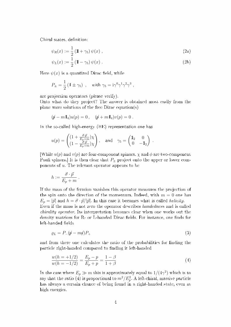
Chiral states, denition:

ψR(x) :=1

2(1l + γ5)ψ(x) , (2a)

ψL(x) :=1

2(1l− γ5)ψ(x) . (2b)

Here ψ(x) is a quantized Dirac eld, while

P± =1

2(1l± γ5) , with γ5 = iγ0γ1γ2γ3 ,

are projection operators (please verify).Onto what do they project? The answer is obtained most easily from theplane wave solutions of the free Dirac equation(s)

(/p −m1l4)u(p) = 0 , (/p +m1l4)v(p) = 0 .

In the so-called high-energy (HE) representation one has

u(p) =

((1 + ~σ·~p

Ep+m)χ

(1− ~σ·~pEp+m

)χ

), and γ5 =

(1l2 00 −1l2

).

[While u(p) and v(p) are four-component spinors, χ and φ are two-componentPauli spinors.] It is then clear that P± project onto the upper or lower com-ponents of u. The relevant operator appears to be

h :=~σ · ~p

Ep +m.

If the mass of the fermion vanishes this operator measures the projection ofthe spin onto the direction of the momentum. Indeed, with m = 0 one hasEp = |~p| and h = ~σ · ~p/|~p|. In this case it becomes what is called helicity.Even if the mass is not zero the operator describes handedness and is calledchirality operator. Its interpretation becomes clear when one works out thedensity matrices for R- or L-handed Dirac elds. For instance, one nds forleft-handed elds

%L = P−(/p −m/s)P+ (3)

and from there one calculates the ratio of the probabilities for nding theparticle right-handed compared to nding it left-handed

w(h = +1/2)

w(h = −1/2)=Ep − p

Ep + p=

1− β

1 + β(4)

In the case where Ep m this is approximately equal to 1/(4γ2) which is tosay that the ratio (4) is proportional to m2/E2

p . A left-chiral, massive particlehas always a certain chance of being found in a right-handed state, even athigh energies.

4

Summary of lecture 2 (4 March 2010)

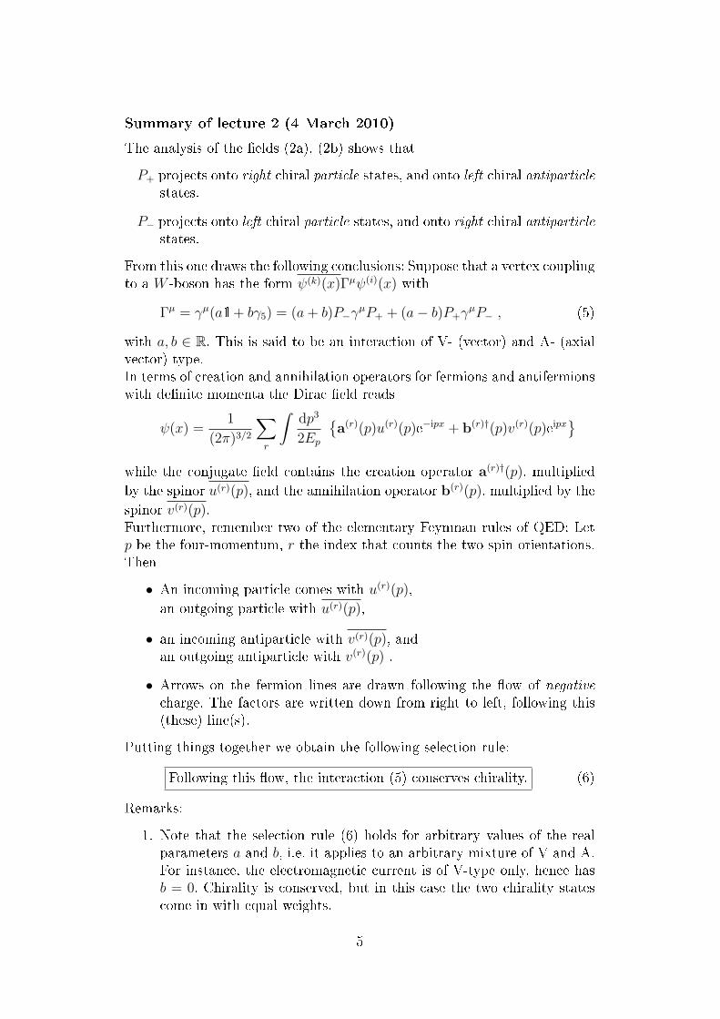
The analysis of the elds (2a), (2b) shows that

P+ projects onto right chiral particle states, and onto left chiral antiparticlestates.

P− projects onto left chiral particle states, and onto right chiral antiparticlestates.

From this one draws the following conclusions: Suppose that a vertex couplingto a W -boson has the form ψ(k)(x)Γµψ(i)(x) with

Γµ = γµ(a1l + bγ5) = (a+ b)P−γµP+ + (a− b)P+γ

µP− , (5)

with a, b ∈ R. This is said to be an interaction of V- (vector) and A- (axialvector) type.In terms of creation and annihilation operators for fermions and antifermionswith denite momenta the Dirac eld reads

ψ(x) =1

(2π)3/2

∑r

∫dp3

2Ep

a(r)(p)u(r)(p)e−ipx + b(r)†(p)v(r)(p)eipx

while the conjugate eld contains the creation operator a(r)†(p), multiplied

by the spinor u(r)(p), and the annihilation operator b(r)(p), multiplied by the

spinor v(r)(p).Furthermore, remember two of the elementary Feynman rules of QED: Letp be the four-momentum, r the index that counts the two spin orientations.Then

• An incoming particle comes with u(r)(p),

an outgoing particle with u(r)(p),

• an incoming antiparticle with v(r)(p), andan outgoing antiparticle with v(r)(p) .

• Arrows on the fermion lines are drawn following the ow of negativecharge. The factors are written down from right to left, following this(these) line(s).

Putting things together we obtain the following selection rule:

Following this ow, the interaction (5) conserves chirality. (6)

Remarks:

1. Note that the selection rule (6) holds for arbitrary values of the realparameters a and b, i.e. it applies to an arbitrary mixture of V and A.For instance, the electromagnetic current is of V-type only, hence hasb = 0. Chirality is conserved, but in this case the two chirality statescome in with equal weights.

5

2. If one considers a vertex of S- (scalar) and P- (pseudoscalar) type in-stead, Γ = c1l + dγ5, one sees that the chirality ips at every suchvertex.

1.3 Example: Two-body decays of charged pions

A remarkable example is provided by the decays π+ → e+νe and π+ → µ+νµ.

Assume the vertex (5) to have a = −b = 1 (the case of V-A interaction), andassume the neutrinos to be massless. In this case the neutrinos are L-chiral,the positron and the µ+ are R-chiral. The neutrino being massless, its spinis fully aligned in a direction opposite to the momentum. In contrast to this,the R-chirality of the charged partner means that it has a large componentwhere the spin is aligned along the momentum, and a small component whereit is aligned antiparallel to the momentum in the ratio m2

f/m2π, cf. (4),

f denoting the charged lepton.Angular momentum conservation implies that the three-component J3 of thetotal angular momentum is conserved. As all partial waves of the plane wavedescribing the outgoing charged lepton and neutrino have m` = 0 (if therelative momentum is taken to be the 3-axis), and as J3 = 0 before the

decay, one obtains m(f)s +m

(νf )s = 0 with f = e or f = µ.

Obviously, this selection rule is only obeyed by the small component of thecharged lepton's chiral eld. Thas is to say, if the charged lepton were mass-less, too, the decay would not take place at all. This clash between the chi-rality selection rule for V and A interactions and angular momentum conser-vation explains the smallness of the branching ratio (1).As an exercise repeat the analogous analysis for the case a = b = 1, i.e.for a pure V+A vertex. The conclusions are the same. This shows that anymixture of vector and axial vector interaction will lead to the suppressionof the decay into the lighter of the charged leptons. This seems reasonablebecause rates cannot depend on relative signs, i.e. cannot distinguish V +Afrom V − A.

1.4 Muon decay as a model system for charged weak interactions

Muon decay µ− → e− νe νµ is one of the elementary and most instructivedecay processes in weak interactions. Muons are produced abundantly indecays π− → µ−νµ, where the newly born muons possess polarization Pµ.The kinematics of muon decay yields the following range of the energy E ofthe electron

me ≤ E ≤ W =m2

e +m2µ

2mµ

or x0 ≤ x ≤ 1 where x :=E

W, x0 =

me

W.

Clearly, unless one is interested in the extreme lower end of the spectrum,one may assume x to scan the interval 0 ≤ x ≤ 1.

6

Remark: Of course, we know that this decay is due to exchangeof a W -boson between the (µ, νµ)- and (e, νe) vertices. The eectof the mass of theW through its propagator on the muon's decaywidth is found to be (exercise!)

Γ = Γ(mW →∞)

1 +

3

5

m2µ

m2W

.

The correction is very tiny. Therefore, the W -propagator may beshrunk to a point, so that the interaction eectively becomes afour-fermion contact interaction.

As, a priori, one does not know the details of the interaction, one tries alladmissible coupling terms, each one characterized by a coupling parameter.This analysis, originally due to Louis Michel, yields the following expressionfor the double-dierential decay width

d2Γ

dxd(cos θ)= A

m5µG

2F

210π36x2[

6(1− x) + 43%(4x− 3)

]+ Pµξ cos θ

[2(x− 1) + 4

3δ(3− 4x)

]+ . . .

. (7)

The terms omitted are important only at the low end of the spectrum, ordepend on the spin orientation of the electron. The real parameters A, %, ξ,δ, and a few more are linear combinations of squares of coupling constants(not given here). In case of V-A they are A = 16, % = δ = 3/4, ξ = 1, etc.These values are conrmed in a series of precision experiments (for detailssee pdg.lbl.gov). Typical results are

% = 0.7503± 0.0004 , δ = 0.7504± 0.0006 ,

ξPµ = 1.007± 0.0035 , η = 0.001± 0.024 .

Eq. (7) yields interesting information around the upper end of the spectrum.Indeed, one nds from (7)(

d2Γ

dx d cos θ

)∣∣∣∣x→1

=m5

µG2F

144π3%

1− Pµ

ξδ

%cos θ

,

An experiment which measured this quantity found

Pµξδ

%= 0.9989± 0.0023 .

By denition, the longitudinal polarization Pµ cannot be larger than 1. Also,from the denitions in terms of coupling constants, the absolute value ofthe combination (ξδ/%) cannot exceed the value 1. One concludes that bothPµ and the combination ξδ/% must each lie very close to 1. The result forthe former has an immediate consequence for the chirality of the νµ of the

7

antineutrino emitted in pion decay, by conservation of angular momentum,the experimental result given above implies

1− 2|h(νµ)| < 0.0032 at 90% C.L. .

The signs of h(νµ) and h(νµ), which are opposite of each other, are knownfrom another experiment. Therefore, the result is convertible to the informa-tion

h(νµ) = +1

2and h(νµ) = −1

2, (8)

within very small error bars. This is, by far, the most accurate determinationof a neutrino helicity. Note that in case of spin-1/2 it is customary to denethe helicity twice these values, i.e. h(νf ) = +1 and h(νf ) = −1.

In summary:

Charged Current (CC) weak interactions couple to L-chiral eldsonly. Neutrinos (antineutrinos), as long as they are consideredmassless, couple only by left-helicity (right-helicity).There are Neutral Current (NC) weak interactions as well towhich we will turn later.

2 Mass sectors of leptons and quarks

Summary of lectures 3 and 4 (9 and 11 March 2010)

2.1 Mass matrices and mixing

With Ψ(x) a multi-component fermion eld containing all leptons (or quarks)of equal charge, the Lagrange density will have the form

L = Ψ(x) (iγµ∂µ −M) Ψ(x) + h.c. , (9)

where M is a matrix which need neither be hermitean nor diagonal. It willnot be diagonal if Ψ refers to a basis of weak interaction eigenstates and ifthese do not coincide with the mass eigenstates.

The mass matrix is a Lorentz-scalar. With regard to the space of Diracspinors, the decomposition in terms of L- and R-chiral elds shows that themass term is of the form −Lmass = ΨRMΨL + h.c.. Indeed, one has

ΨR/L = (P±Ψ)†γ0 = Ψ†P±γ0 = Ψ†γ0P∓ = ΨP∓ , hence

ΨΨ = (ΨR + ΨL)(ΨR + ΨL) = Ψ(P− + P+)(P+ + P−)Ψ ,

of which only the cross terms survive. Note that the CC weak interactionscouple to L-elds only and are blind to the R-elds.

8

Introduce the following notation: For weak interaction states let the Diracspinors for particles with the higher value of the electric charge be denotedgenerically by u(i)(x), for particles with the lower electric charge by d(i)(x),the superscript i = 1, 2, 3 counts the families or generations. So, in the caseof leptons, the particles with electric charge Q = 0 are the neutrinos, whilethe ones with Q = −1 are the charged leptons e−, µ−, and τ−. In the caseof quarks u(i) stands for the three up-quarks with charge +4/3, d(i) standsfor the three down quarks with charge −1/3, as they appear in CC weakinteractions.More explicitly, the mass sector in the Lagrangian has the form

−Lmass = 12

3∑

i,k=1

u(i)L M

(u)ik u

(k)R +

3∑i,k=1

d(i)L M

(d)ik d

(k)R

+ h.c. . (10)

The two mass matrices that appear here, are diagonalized by bi-unitary trans-formations,

U(u)L M (u)U

(u)R = D(u) and U

(d)L M (d)U

(d)R = D(d) , with

D(u) = diag (m(u)1 ,m

(u)2 ,m

(u)3 ) and D(d) = diag (m

(d)1 ,m

(d)2 ,m

(d)3 ) .

These formulae depend on four independent unitary matrices. It is not dif-cult to verify that the determination of these unitaries can be reduced todiagonalization of hermitean matrices, (dropping the superscripts (u) or (d))

UR

(M †M

)U †

R = D2 = UL

(MM †)U †

L .

The corresponding eigenstates are the mass eigenstates. We denote the L-chiral eigenstates by t

(i)L and b

(i)L in the two charge sectors, respectively. They

are

t(i)L =

∑k

(U

(u)L

)iku

(k)L , b

(i)L =

∑k

(U

(d)L

)ikd

(k)L . (11)

Note that the CC weak interaction vertices are proportional to

u(i)L γ

µ(1l− γ5)d(k)L .

Therefore, when expressed in terms of mass eigenstates, these vertices arecharacterized by the mixing matrix

U(u)L U

(d)†

L =: V . (12)

In the case of quarks V ≡ VCKM is the Cabibbo-Kobayashi-Maskawa mixingmatrix. In the case of leptons it has no generally accepted name.

9

2.2 Some comments

1. In the case of quarks the mass eigenstates are the states which are char-acterized by quantum numbers such as strangeness, etc., all of which areconserved in strange interactions but not in CC weak interactions. Themixing matrix may hence be visualized as a kind of rotation betweenstates participating in strong interactions and states participating inCC weak interactions.

2. Number of observable parameters in V : Being unitary, V a priori de-pends on nine real parameters. As ve relative phases (six minus oneoverall phase) can be absorbed in the initial and nal states, there re-main four observable variables. With three generations one takes themto be three real mixing angles θ1, θ2, θ3 and one (real) phase angle φ.

3. It is instructive to consider the most general transformation whichleaves V invariant:Let U , W (u), and W (d) be arbitrary unitary matrices. Then the simul-taneous transformations of the mass matrices

U †M (u)W (u) and U †M (d)W (d) (13)

leave V , eq. (12), unchanged (please verify!).

4. While the route from a set of given matrices to the mixing matrix isclear, it is of interest to determine the set of all mass matrices thatare compatible with a set of given data, i.e. with the three massesm1,m2,m3 and the four observables derived from the mixing matrix V .(For details and references see FS's talk at Villa de Leyva summerschool 2010, accessible through web page.) This may be useful for modelbuilders.

5. In relation to the previous comment it useful to know that by a suitablechoice of basis states one can transform any set of mass matrices to theform

M =

0 ∗ 0∗ 0 ∗0 ∗ ∗

where the asterisks indicate nonvanishing entries. In the literature onthe subject this is called the NNI representation (for "nearest neighbourinteractions"). Although this is a useful representation in analyses ofmass matrices, the name is misleading because it suggests a specicpattern in the interaction responsible for the mass sectors, althoughthere is none.

6. It is obvious that by making use of the freedom (13) the mixing canbe shifted from one charge sector to the other, or may even be split

10

between the two charge sectors. Note that by convention one takesthe down-quarks to be the mixed states in the quark sector, and theneutrinos to be the mixed states in the leptonic sector.

3 Geometric Constructionof Non-Abelian Gauge Theories

Summary of lectures 5 and 6 (16 and 18 March)

3.1 Ideas and expectations

Matter: Leptons are classied as described above, i.e. doublets for L-elds,and singlets for R-elds(

νe

e−

)L

, e−R

(νµ

µ−

)L

, µ−R

(ντ

τ−

)L

, τ−R , (14a)

With respect to the U(1) factor in the group U(2)'UY (1)×SUI(2) thedoublets have Y = −1, the singlets have Y = −2, so that the electriccharge is given by Q = I3 + 1

2Y .

Quarks appear in three copies of the reducible multiplet containing aSU(2)I doublet and two singlets,

Ψ(1) =

(uL

dL

)uR

dR

Ψ(2) =

(cLsL

)cRsR

Ψ(3) =

(tLbL

)tRbR

(14b)

Up-quarks have electric charge Q = +23, down-quarks have Q = −1

3.

The weak hypercharges of the doublets are Y = 13, uR, cR, and tR have

Y = 43, while dR, sR, and bR have Y = −2

3. One veries their electric

charges by the formula Q = I3 + 12Y .

Aims: Want to incorporate: The neutral-current (NC) phenomenology ofelectromagnetic and weak interactions, the maximal violation of parityin CC interactions, the phenomenology and structure of QCD. (Re-garding the latter subject, we repeated the motivation for the colourdegrees of freedom as obtained from the constituent quark model andthe spin-statistics relation for quarks.)Following the model of quantized Maxwell theory (QED) as a success-ful, predictive renormalizable quantum eld theory, quest for a renor-malizable unied theory.

11

Table 1: Quantum numbers of leptons (L=Le+Lµ+Lτ )

Q L Le Lµ Lτ I3 Y(νe)L 0 1 1 0 0 +1

2-1

(e−)L -1 1 1 0 0 −12

-1(e−)R -1 1 1 0 0 0 -2

(νµ)L 0 1 0 1 0 +12

-1(µ−)L -1 1 0 1 0 −1

2-1

(µ−)R -1 1 0 1 0 0 -2

(ντ )L 0 1 0 0 1 +12

-1(τ−)L -1 1 0 0 1 −1

2-1

(τ−)R -1 1 0 0 1 0 -2

The two tables summarize the quantum numbers of leptons and quarks asdiscussed above. The last two columns show the weak isospin and weak hyper-charge assignments which are relevant for the electroweak (minimal) standardmodel. Note that the electric charge is Q = I3 + 1

2Y .

Table 2: Quantum numbers of quarks

Q B C S To Bo I3 YuL

23

13

0 0 0 0 +12

+13

dL -13

13

0 0 0 0 −12

+13

uR23

13

0 0 0 0 0 +43

dR -13

13

0 0 0 0 0 −23

cL23

13

1 0 0 0 +12

13

sL -13

13

0 -1 0 0 −12

13

cR23

13

1 0 0 0 0 +43

sR -13

13

0 -1 0 0 0 −23

tL23

13

0 0 1 0 +12

13

bL -13

13

0 0 0 -1 −12

13

tR23

13

0 0 1 0 0 +43

bR -13

13

0 0 0 -1 0 −23

12

3.2 Geometry of Maxwell theory

The relevant elds are the four-potential Aµ(x) and the eld strength tensoreld F µν(x), which, when expressed in a given frame of reference, are

Aµ(x) =(Φ(t, ~x), ~A(t, ~x)

)T

, F µν(x) =

0 −E1 −E2 −E3

E1 0 −B3 B2

E2 B3 0 −B1

E3 −B2 B1 0

. (15)

The homogeneous and inhomogeneous Maxwell equations (in vacuum) read,respectively,

∂λF µν(x) + (cyclic permutations of λ, µ,ν) = 0 , (16a)

∂µFµν(x) = 0 . (16b)

Gauge invariance: If Aµ(x) 7→ A′µ(x) = Aµ(x)−∂µχ(x), with χ(x) a Lorentzscalar function (which is at least C2), the eld strength tensor and hence theelectric and magnetic elds remain unchanged.

Example: Consider the Schrödinger equation for a charged particle subjectto external electric and magnetic elds, the Hamiltonian being

H =1

2m

[~p− e

c~A]2

+ eΦ .

If one performs a time and space dependent phase transformation onthe wave function by means of an arbitrary smooth function α(t, ~x)

ψ(t, ~x) 7−→ ψ′(t, ~x) = eiα(t,~x)ψ(t, ~x) (17a)

then the equation of motion remains unchanged if one performs simul-taneously a gauge transformation of the elds by means of the gaugefunction

χ(t, ~x) =~ceα(t, ~x) . (17b)

(Work this out as an exercise.) This reationship was found by V. Fockin 1926. It shows very clearly that in the case of Maxwell theory therelevant symmetry group is G =U(1).

Let M denote Minkowski space, i.e. the space R4 equipped with the metricg = diag (1,−1,−1,−1), let Λ∗ = ⊕kΛ

k be the space of exterior forms onM , and d : Λk → Λk+1 the exterior derivative.Dene the following one- and two-forms, respectively,

ωA := Aµ(x)dxµ , ωF :=∑µ<ν

Fµνdxµdxν . (18)

13

One veries easily that ωF = dωA is identical with the well-known expressionFµν(x) = ∂µAν(x) − ∂νAµ(x) which guarantees the validity of the homoge-neous equations (16a). A gauge transformation takes the form

ωA 7−→ ωA′ = ωA + dχ(x) =⇒ ωF ′ = ωF .

The covariant derivative which acts on matter elds (bosonic or fermionic)is

DA := d + iq

~cωA = i

(−id +

q

~cωA

)(19)

where the second form reminds one of (~p− qc~A) with ~p = −i~∇.

Of course, one chooses units such that ~ = 1 and c = 1. It is convenient toabsorb the factor i and the coupling constant q (which is the electric chargein the case of Maxwell theory) in the denition of the exterior forms (18),

A := iq

~cωA , F := i

q

~cωF . (20)

Then the above denitions are rewritten as follows

DA = d + A , F = dA , and one calculates

D2A = (d + A) (d + A) = d d + dA+ Ad

= (dA)− Ad + Ad = (dA) = F ,

where d2 = 0 and the graded Leibniz rule for the exterior derivative wereused. The covariant derivative acts on bosonic or fermionic elds, DAΦ orDAΨ, scalar products such as (DAΨ, DAΨ) will be invariant under gaugetransformations A 7→ A′ = A+ dΛ provided the action of G on the eld is

Ψ(x) 7→ Ψ′(x) = g(x)Ψ(x) with g(x) = eΛ .

3.3 Compact non-Abelian groups and their algebras

One starts from the structure group G and its Lie algebra g ≡ Lie(G). HereG is a compact Lie group, simple or semi-simple.The generators of g aredenoted by Ti, and they fulll the commutators (summation over repeatedindices is implied)

[Ti, Tj] = iCkijTk . (21)

From the Jacobi identity for the generators one deduces the following relationfor the structure constants

Cmij C

lmk + Cm

jkClmi + Cm

kiClmj = 0 .

Among the irreducible, unitary representations most important for our con-struction is the adjoint representation, where the generators are representedby the matrices

U(ad)lm (Tk) = −iCm

kl .

14

(Exercise: Verify that these matrices do indeed fulll the commutators (21).)The Killing metric is dened by

gij := tr(U (ad(Ti)U

(ad(Tj))

= −CpiqC

qjp (22)

Finally, by the denition Cijk := Cpijgpk one obtains the structure constants

in a form where they are antisymmetric in all three indices. (Verify this bymeans of the identity derived from the Jacobi identity!)An important property which is used in the construction of local gauge theoryis the following: By suitable linear combination the generators can be chosensuch that

tr (U(Ti)U(Tj)) = κδij , (23)

where the real constant κ depends on the representation but is independentof the generators Ti. (We gave a proof of this fact.)The example of SU(2):

Ti =σi

2, σ1 =

(0 11 0

), σ2 =

(0 −ii 0

), σ3 =

(1 00 −1

),

yields the fundamental representation for which κ(fund) = 1/2.The adjoint representation is given by

U (ad)(T1) = −iε1lm = −i

0 0 00 0 10 −1 0

=

0 0 00 0 −i0 i 0

,

U (ad)(T2) =

0 0 i0 0 0−i 0 0

, U (ad)(T3) =

0 −i 0i 0 00 0 0

,

from which one calculates κ(ad) = 2.

3.4 Globally and locally invariant Lagrange densities

With G denoting the structure group, construct the principal bre bundle(M,G) with base manifold M = R4 and typical ber G. This constructionalso denes the innite dimensional gauge group G (loosely speaking: to eachpoint x ∈ M a copy xG of the structure group is attached). Dene the Liealgebra-valued one-form, with N = dim Lie(G),

A := iqN∑

k=1

A(k)Tk with Ak = A(k)µ (x)dxµ, k = 1, 2, . . . , N, (24)

In any reducible or irreducible representation of G spanned by the compo-nents of some (bosonic or fermionic) matter eld Φ, A will be realized by amatrix U(A) = iq

∑Nk=1A

(k)U(Tk). For example, if Φ spans anm-dimensionalrepresentation, these will be m×m matrices.

15

The one-form A is called connection form. Indeed, it describes parallel trans-port of the eld Φ from x to x+ dx,

φ(x+dx)i =

m∑j=1

δij − Uij(A)φ(x)j ,

provided A transforms under a gauge transformation g(x) ∈ G as follows

A 7−→ A′ = gAg−1 + g(dg−1) . (25)

Schematically this is shown as follows. A natural requirement is that paralleltransport should commute with the action of a gauge transformation, that isto say, one should have

g(x+ dx)(1l− A) = (1l− A′)g(x) . (26)

Upon Taylor expansion to rst order, g(x+dx) ' g(x)+dg(x), eq. (26) gives

dg − gA = −A′g or A′ = gAg−1 − (dg)g−1 .

Note that d(gg−1) = 0 = (dg)g−1 + g(dg−1) which proves (25).Next one denes the covariant derivative

DA := d + A , (27)

in complete analogy to Maxwell theory, as well as the curvature two-form

F := (dA) + A ∧ A . (28)

Note that in the case of Maxwell theory the structure group was G =U(1),and the second term on the right-hand side in (28) vanished. Furthermore,

D2A = (d + A) (d + A) = dA+ Ad + A ∧ A = (dA) + A ∧ A = F .

We showed that under a gauge transformation DA transforms by "conjuga-tion", DA 7→ DA′ = gAg−1. As F = D2

A, this is also true for the curvature;F 7→ F ′ = gFg−1. This will be important when we will have to constructinvariants under the gauge group G.The term in F which is new as compared to Maxwell theory is

A ∧ A = −q2

N∑k,l=1

TkTl

3∑σ,τ=0

A(k)σ (x)A(l)

τ (x) dxσ ∧ dxτ

= −q2

N∑k,l=1

[Tk, Tl

]∑µ<ν

A(k)µ (x)A(l)

ν (x) dxµ ∧ dxν

= −iq2

N∑k,l,m=1

CklmTm

∑µ<ν

A(k)µ (x)A(l)

ν (x) dxµ ∧ dxν .

16

Obviously, F is a Lie algebra-valued two-form. Therefore, it is natural towrite it as a linear combination F = iq

∑k Tk

∑µ<ν F

(k)µν (x) dxµ ∧ dxν in

terms of the generators. The coecients in this expression are the followingfunctions

F (k)µν (x) = ∂µA

(k)ν − ∂νA

(k)µ − q

N∑m,n=1

CkmnA(m)µ (x)A(n)

ν (x) . (29)

The rst term on the right-hand side is the same as for the Maxwell eld.The second term is new and is typical for non-Abelian theories.The Lagrange density for a gauge theory with matter must be globally invari-ant (i.e. with respect to the structure group G) and locally invariant (i.e.withrespect to the gauge group G). Its generic structure will be

L = LYM + LΦ + LΨ , where

LYM = − 1

4q2κ(ad)tr (FµνF

µν) , (30a)

LΦ = 12

(DAΦ, DAΦ)− µ2 (Φ,Φ)

−W (Φ) , (30b)

LΨ = i2

(Ψ, γα

↔Dα Ψ

)−(Ψ, (M + gΦ)Ψ

). (30c)

The "left-right" notation of the covariant derivative in (30c) is a short-handfor Ψ(DαΨ)− (DαΨ)Ψ. The "bracket" notation (· · · , · · · ) is somewhat sym-bolic. It is meant to indicate that the two objects on the right and on theleft should be coupled to a scalar with respect to G (global invariance!). For

example, if G =SO(3) and ~Φ = φ1, φ2, φ3 is a triplet, (Φ,Φ) stands for

the scalar product (~Φ · ~Φ). Likewise, if G =SU(3) and Ψ is an octet 8, thenΨ (which is the conjugate octet) and Ψ must be coupled according to theClebsch-Gordan series 8⊗8 → 1. In this way all terms in L are G-invariant.

3.5 The U(2) model of electroweak interactions

Summary of lectures 6 and 7 (23 and 25 March)The generators of the Lie algebra of U(2) are taken to be

T0 = 1l2 ≡ σ0, Ti = 12σi .

It is convenient to replace T1 and T2 by the ladder operators T± = T1 ± iT2.This implies that the corresponding gauge elds are replaced by

W±µ (x) = 1√

2A(1)

µ (x)± iA(2)µ (x) .

and will serve to describe the two charge states of the W -boson. The Yang-Mills Lagrangian (30a) contains the terms

T1A(1)µ (x) + T2A

(2)µ (x) = 1√

2

T−W

(+)µ + T+W

(−)µ

. (31)

17

It also contains neutral terms A(0)µ pertaining to the U(1) factor in G, and

A(3)µ corresponding to the 3-component of SU(2). The physical photon and

Z0 are expected to be linear combinations thereof, viz.

A(γ)µ (x) = A(0)

µ (x) cos θW − A(3)µ (x) sin θW , (32a)

A(Z)µ (x) = A(0)

µ (x) sin θW + A(3)µ (x) cos θW , (32b)

with θW an angle remaining undetermined at this stage, called Weinberg

angle. The neutral sector of LYM then becomes

A(Z)µ (x) (T3 cos θW + T0 sin θW)+A(γ)

µ (x) (−T3 sin θW + T0 cos θW) . (32c)

So far, all vector bosons of the theory are massless. (Adding ad-hoc terms

quadratic in W±µ and A

(Z)µ does not help because such terms are not gauge

invariant.) They have a chance of obtaining masses without destroyinggauge invariance only via LΦ, eq. (30b), in the case where in the lowest(vacuum) state Φ has a nonvanishing value Φ0. Then, indeed, the covariantderivative terms in (30b) will yield mass terms for some or all of the vectorbosons. However, if this happens, we must make sure that the photon remainsmassless! This can only be achieved if the eigenvalues of T0 and T3 in thestate Φ0 are such that in the above decomposition the coecient multiplyingA

(γ)µ (x) vanishes.

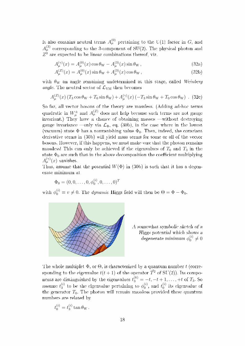
Thus, assume that the potential W (Φ) in (30b) is such that it has a degen-erate minimum at

Φ0 = (0, 0, . . . , 0, φ(i)0 , 0, . . . , 0)T

with φ(i)0 ≡ v 6= 0. The dynamic Higgs eld will then be Θ = Φ− Φ0.

A somewhat symbolic sketch of a

Higgs potential which shows a

degenerate minimum φ(i)0 6= 0

The whole multiplet Φ, or Θ, is characterized by a quantum number t (corre-

sponding to the eigenvalue t(t+ 1) of the operator ~T 2 of SU(2)). Its compo-

nents are distinguished by the eigenvalues t(k)3 = −t,−t+ 1, . . . ,+t of T3. So

assume t(i)3 to be the eigenvalue pertaining to φ

(i)0 , and t

(i)0 its eigenvalue of

the generator T0. The photon will remain massless provided these quantumnumbers are related by

t(i)0 = t

(i)3 tan θW .

18

Regarding the W± and the Z0, the terms in Φ0 that follow from (30b) arethen (

U (Φ)(Aµ)Φ0, U(Φ)(Aµ)Φ0

)= q2

12

(Φ0, U

(Φ)(T+T− + T−T+)Φ0

)W (−)

µ (x)W (+)µ (x)

+(Φ0, U

(Φ)(T3 cos θW + t(i)3 sin θW tan θW)2Φ0

)A(Z)

µ (x)A(Z)µ(x).

Of course, the operator T3 in the third line can be replaced by its eigenvaluet(i)3 and, similarly, the sum of products of ladder operators in the second linecan be replaced by diagonal operators. Indeed, taking account of

12(T+T− + T−T+) = ~T 2 − T 2

3 and of

cos θW + sin θW tan θW =1

cos θW

,

one obtains genuine mass terms for the W± and for the Z0 as follows(U (Φ)(Aµ)Φ0, U

(Φ)(Aµ)Φ0

)= q2v2

[t(t+ 1)− t

(i) 23

]W (−)

µ (x)W (+)µ (x) +

t(i) 23

cos2 θW

A(Z)µ (x)A(Z)µ(x)

.

From his expression one deduces that

m2W ∝ 1

2q2v2

[t(t+ 1)− t

(i) 23

]and m2

Z ∝ q2v2 1

cos2 θW

t(i) 23 ,

from which follows a relation which contains only experimental quantities onone side, only the quantum numbers of φ

(i)0 on the other,

m2W

m2Z cos2 θW

=t(t+ 1)− t

(i) 23

2t(i) 23

. (33)

The left-hand side of (33) is known to be 1 within a very small experimentalerror bar. One veries that the right-hand side takes that value for t = 1

2and

t(i)3 = ±1

2. Here a number of remarks should be made.

1. The component φ(i) of Φ which develops this vacuum expectation valueφ

(i)0 = v must be uncharged. This is achieved by the relation t

(i)0 =

t(i)3 tan θW obtained above. Turning back to the photon coupling in (32c)one sees that it can be written as

(−q sin θW)[T3 − T0

cos θW

sin θW

].

The factor in front is the elementary charge −q sin θW = e. If one wantsto recover the formula Q = T3 + 1

2Y , then the U(1) generator must be

rescaled by dening

Y = −2cos θW

sin θW

T0 . (34)

19

This is always possible because this factor is a U(1) symmetry for whichthe eigenvalues have no scale.

2. Note that the original symmetry is broken from U(2)∼UY (1)×SUI(2)to the residual symmetry UMaxwell(1) of Maxwell theory. The Lagrangedensity still has the full symmetry, the ground state has only the resid-ual symmetry.

3. This reduction or "hiding" of the symmetry has a nice geometric inter-pretation in the framework of Goldstone's theorem.

4. Returning to the explicit expression (29) one realizes that the vectorboson sector (30a) of the Lagrange density contains cubic and quarticcouplings among vector bosons. These are genuine interaction termswhich are new and which are characteristic for non-Abelian theories.For example, these terms x the anomalous magnetic moment of theW -boson through the interaction term with the photon.Joining the SUc(3) of QCD to the gauge group and thereby adding theeight massless gluons to the sector of vector bosons, the LagrangianLYM contains three- and four-gluon couplings. These were tested suc-cessfully in jet physics.

5. A U(1) gauge theory such as Maxwell's theory does not have such self-interactions of the (only) vector boson. Indeed, light-by-light scatteringis possible only in fourth order of QED, via a box diagram involvingfour internal fermion lines (Delbrück scattering).

3.6 SU(3)c and Quantum ChromoDynamics (QCD)

Building stones of QCD are the structure group G =SU(3)c, the colour group,together with the corresponding gauge group, and Ψ : qA,α(x), the quarkelds. Here A = u, d, c, s, t, b is the avour index, α = 1, 2, 3 (or red, white,and blue) is the colour index. The index α corresponds to the triplet repre-sentation 3 of SU(3)c, three-quark states are classied by the singlet of theClebsch-Gordan series

3⊗ 3⊗ 3 = 1a ⊕ 8⊕ 8⊕ 10s .

As the singlet representation is totally antisymmetric in its three factorsthe conict of the quark model with the spin-statistics relation is resolved.Indeed, with εαβγ being an invariant tensor in SU(3), a baryon state is con-structed by taking

3∑α,β,γ=1

εαβγqA,αqB,βqC,γ ,

where the avour quantum numbers A,B,C must be composed such as toyield the correct quantum numbers of the baryons. So, even if the avour

20

state is totally symmetric, and if the orbital wave function is symmetric, too,the total wave function will be antisymmetric by virtue of the colour wavefunction. As an example reconsider the state of a ∆++ with spin projectionms = 3/2:

(u↑u↑u↑) is replaced by3∑

α,β,γ=1

εαβγ(uα↑u

β↑u

γ↑) .

The group G =SU(3) is generated by the eight generators Tk of its Lie algebra

g ∈ SU(3) : g = expih with h =8∑

k=1

αkTk (hermitean).

The dimension of the Lie algebra is 8, the rank of the group is 2. The com-mutators are

[Ti, Tk] = i8∑

l=1

fiklTl , i, k = 1, 2, . . . , 8 , (35)

the structure constants (in totally antisymmetric form) being as follows,

Table 3: Structure constants for SU(3)

ikl 123 147 156 246 257 345 367 458 678

fikl 1 12

−12

12

12

12

−12

√3

2

√3

2

All other constants are either obtained from these by the antisymmetry in(i, k, l), or they vanish, fmnp = 0 in case (m,n, p) is not a permutation of the(i, k, l) listed in the table. In the dening (or fundamental) representationthe generators can be expressed in terms of the Gell-Mann matrices λk, Tk =λk/2, where

λ1 =

0 1 01 0 00 0 0

, λ2 =

0 −i 0i 0 00 0 0

, λ3 =

1 0 00 −1 00 0 0

,

λ4 =

0 0 10 0 01 0 0

, λ5 =

0 0 −i0 0 0i 0 0

, λ6 =

0 0 00 0 10 1 0

,

λ7 =

0 0 00 0 −i0 i 0

, λ8 =1√3

1 0 00 1 00 0 −2

.

In the fundamental representation 3 one has

tr (TiTk) =1

4tr (λiλk) =

1

2δik , hence κ(fund) =

1

2.

21

The adjoint representation is dened by (Tk)mn = −ifkmn, the structureconstants being given by Table 3. The relevant κ parameter is calculated by

tr(T 2

i

)= −

8∑m,n=1

fimnfinm = +8∑

m,n=1

f 2imn giving κ(ad) =

3

2.

The QCD-Lagrangian is then constructed as formulated in eqs. (29) and(30a). It describes 8 massless vector bosons, the gluons which are interpretedas the carriers of strong interactions. However, while the Lagrange functionfor QCD is simple, its ground state is a highly correlated state (connement! ).

4 The minimal standard model and beyond

4.1 Some comments

1. The standard model works all too well: The model as such, as well as theradiative corrections it allows to calculate, were brillantly conrmed bythe precision data obtained at LEP and at the Tevatron. Global ts toall data (masses ofW and Z, their widths ΓW and ΓZ , various forward-backward asymmetries in the neighbourhood of the Z-pole in e+e−

scattering, etc.) are of high quality and leave no room for deviationsfrom the minimal version of the standard model.

As we explained in detail, the standard model is a parametrization andsummary of the empirical knowledge of its building blocks and their in-teractions at low energies (maximal parity violation in CC-interactions,neutral current phenomenology, neutrinos being pure L-elds, etc.).

2. The model is free of anomalies. Although it exhibits a U(1) anomaly(which manifests itself in the succesful prediction of the π0 → γγ decayrate), the contribution of the three lepton families cancels the contri-bution of the three families of (coloured) quarks (see below, Sect. 4.3).As a consequence, the model can be quantized in a consistent mannerso that radiative corrections are nite and well-dened.

3. The model, unfortunately, contains too many free parameters (some 24in all!). An example is provided by the fermionic mass sector: As weshowed in the lectures there can be no genuine fermion masses becausethey cannot be reconciled with gauge symmetry. It is not possible toform a G-scalar from a L-chiral eld, which is a member of a doublet,and a R-chiral eld which is a singlet with respect to SU(2)I . If insteadthe fermions are given their masses by the Higgs mechanism, then theYukawa couplings of the Higgs eld to each lepton or quark must bechosen proportional to the masses one wishes to obtain.As an example consider the L-doublet L(f) = (νf , f

−)T with weak hy-percharge Y = −1, and the R-chiral eld (f−)R with Y = −2, as well

22

as the Higgs doublet Φ with Y = 1. As L(f) then has Y = +1, a Yukawacoupling of the type

LYukawa = g(f)(L(f)Φ

)f−R + h.c.

(36)

is (globally) invariant (which is sucient here): The additive conser-vation of weak hypercharge is respected. The two SU(2)I doublets arecoupled to a scalar. The price one has to pay is that the Yukawa cou-pling constant must be adjusted such as to give the correct fermionmass. Typically, with Φ replaced by Φ0 and with (Φ0,Φ0) = v2 oneobtains

g(f) =mf

vwith v ' 250 GeV.

This "explains" why the couplings to the physical Higgs particle areexpected to be very small and, consequently, why the production ratesof Higgs particles are low.

So one may claim that the standard model does not really unify theinteractions. In essence, it contains too little structure: While it xes thesector of vector bosons to a large extent (self-couplings of non-Abelianvector elds), it leaves much freedom in the choice of multiplets for thematter particles, leptons and quarks. Also, the Higgs sector remainssomewhat enigmatic.

4. There are many attempts to endow the model with more structureby embedding it in larger groups (grand unied theories), or by intro-ducing space-time supersymmetry, or in more exotic versions such astechnicolour, etc. They all have in common that even more parametersare introduced which are not determined, not less.

5. Matters that we did not have time to discuss in more detail:

• BRST symmetry and its implications. The symmetry operationdiscovered by Becchi, Rouet, Stora, and Tyutin is an elegant methodto implement gauge invariance. This operation introduces a fur-ther, graded algebraic and geometric structure which, when com-bined with the requirements of locality and causality à la Epsteinand Glaser, leads to another, deeper perspective of gauge theories.

• Perturbative and nonperturbative regimes of gauge theories.

4.2 Anomalies in gauge theories: Generalities

Geometrically speaking, anomalies are topological obstructions in the con-struction of the action for a Yang-Mills theory. If a gauge theory exhibitsanomalies it cannot be quantized properly, that is to say, the theory will notmake sense at the quantum level, as a renormalizable quantum eld theory.Qualitatively speaking, the reason for this complication is the following.

23

The space A of all connections is an ane space. This would be a fairlysimple and perfectly manageable space were it not for gauge invariance ofnon-Abelian theories. Gauge symmetry means that there are classes of gauge-equivalent connections [A] and, in essence, that the full gauge group G shouldbe divided out. However, the space A/G has a complicated structure and thisdivision must be done more carefully, in a series of steps, while following thefate of the action functional along this procedure. A good way of studyingthis process is to make use of the stratication of the space A by the gaugegroup, the strata being dened by equivalence classes of gauge-equivalentconnections.For that purpose one studies the stratication of A by the action of the gaugegroup, so that it is decomposed as follows

A = A(J0) ∪ A(J1) ∪ · · ·A(Jk) , (37a)

where the individual stratum is characterized by the stability group GA ofits elements A being conjugate to Ji, i = 0, . . . , k. That is to say

A(Ji) =A ∈ A|GA = ψJiψ

−1 , ψ ∈ G. (37b)

Here Ji is isomorphic to a subgroup of the structure group G. The numberof strata is countable. The main stratum (index J0) is characterized by J0

isomorphic to the center C of G. The stratication (37a) is unique and, infact, natural. The formal denition

Mi = A(Ji)/G

yields an orbit bundle decomposition which bears some similarity to thecompactication procedure in Kaluza-Klein theories. The spaces Mi areparts of the space of physical, gauge-inequivalent connections.Physics comes in via an action functional S(A, ψ, ψ) which is a classicalfunctional that is strictly gauge invariant. At the quantum level the centralquantity is the generating function

Z(A) =

∫[Dχ][Dχ] exp−(S + χ /∂A χ) (38)

obtained while integrating the fermionic degrees of freedom. There are twopossibilities. Either Z(A) is strictly invariant under a gauge transformationψ, Z(ψA) = Z(A), or it is equivariant but not strictly invariant, Z(ψA) =%−1(A,ψ)Z(A), where % is the action of the gauge transformation. In therst case one can safely divide by the gauge group to obtain a perfectlyacceptable functional. The theory has no anomaly and can be reduced to thespace M of gauge-inequivalent connections. In the second case, in contrast,there must be anomalies, the reduction is not possible. Therefore, in thegeometric framework anomalies show up as obstructions to the reductionprocedure which are due to quantization.

24

One well-known ansatz is to make use of what is called the pointed gauge

group G∗. This is the subgroup of G which is the stability group of an arbi-trary but xed point p0 of the principal bre bundle P(M,G),

G∗ = Gp0 = ψ ∈ G|ψ(p0) = p0 . (39)

In other terms the pointed gauge group acts like the identity in the breover p0. Singer showed that the action of G∗ on A is free [4]. Therefore,

G∗ −→ A

↓M∗ = A/G∗

is a principal bre bundle. The functional Z(A) is a trivial section

Z : A −→ Det := A× C (40a)

in the determinant bundle. If one divides by the pointed gauge group oneobtains the reduced section

Z∗ : A/G∗ −→ (A× C) /G∗ =: Det ∗ . (40b)

If Z(A) is strictly invariant then the action of G∗ on C is trivial so that (40b)reduces to

Z∗ : M∗ −→M∗ × C , M∗ = A/G∗ . (40c)

In turn, if Z(A) is equivariant but not strictly invariant then the action ofthe pointed gauge group on C is not trivial. In this situation Det∗ has a twist,the integration over [DA] is not possible. Geometrically speaking there is atopological anomaly.Even if no such anomaly is encountered, the story is not nished. Thereremains the "division" by the remainder G/G∗ which is isomorphic to thestructure group G. This last step is particularly important because it is thestructure group which denes the conserved charges of the theory. Again, ifZ∗ is strictly invariant the nal division poses no problem. If it is not but is(only) equivariant one obtains

Z∗∗ : M−→ (M∗ × C) /G =: Det∗∗ , (41)

the functional Z∗∗ is nontrivial, and one has found an anomaly.In summary, by following this geometrical method one identies all topolog-ical as well as possible global, nonperturbative anomalies. More on this canbe found e.g. in [4], and in [5] [7].

4.3 Anomalies: An example

The electroweak sector of the standard model is based on U(2)'U(1)Y×SU(2)I .The SU(2) factor does not yield an anomaly. However, the U(1) part contains

25

a chiral anomaly that was the rst that was discovered in the 1960-ties byAdler, Bell, and Jackiw. This example is instructive for two reasons. First, itshows that anomalies may be there but they may cancel due to the specicfermion content of the model. Second, the axial anomaly, when conned tothe contributions of quarks, may be useful in predicting the decay rate forπ0 → γγ in a quantitative manner.Dene the axial vector current Jµ

A and the axial density JA of some fermioneld(s) as follows

JµA(x) := ψ(x)γµγ5ψ(x) , (42a)

JA(x) := ψ(x)γ5ψ(x) . (42b)

Here ψ may be a single fermion eld ψ ≡ ψ(f), or a multi-component Diraceld ψ(x) ≡ Ψ(x) which contains dierent species of fermions that are dis-tinguished by their quantum numbers.The neutral pion π0 has spin/parity 0−, so that the divergence ∂µJ

µA of the

current (42a) is a suitable interpolating eld for the pion. The process π0 →γγ involves three vertices:

(k,

(k’,

ε)

ε’)

π0

Figure 1: Triangle graph illustrating π0 decay via the axial anomaly

Two vector vertices proportional to γα and γβ at which the two photons(k, ε) and (k′, ε′) are created, respectively, (the rst symbol denoting thefour-momentum, the second the polarization), and the pseudoscalar ∂µJ

µA

describing the dissociation of the π0 into two quarks. From general consider-ations, regarding spin and parity selection rules, the decay amplitude musthave the form

T (π0 → γγ) = F εαβστkαk′βεσε′τ , (43a)

where F is a Lorentz-scalar form factor whose absolute square determinesthe decay width, or inverse lifetime,

τ−1 =m3

π

64π|F |2 . (43b)

Naïvely one would expect that F tend to zero as m2π → 0. "Naïve" here

means that while π0 is described by ∂µJµA, this divergence is calculated by

26

making use of the equations of motion that follow from the Lagrange density,

∂µJµA = 2imJA(x) , (44a)

where m is a quark mass. This calculation is purely formal because onedid not check whether the relevant Feynman diagram is convergent or not.In fact, the triangle diagram is found to be (linearly) divergent and mustbe regularized in order to make sense. If one does so (as was rst done bySt. Adler) one nds instead of (44a)

∂µJµA = 2imJA(x) +

α

4πεαβστF

αβ(x)F στ (x) . (44b)

The second term in (44b) is said to be the axial anomaly. We return to it andto its use for π0-decay further below. For the moment we consider the moregeneral case of a triangle graph with two vector currents and one axial-vectorcurrent, but allow both leptons and quarks to circulate along the loop. Onethen shows that if there were only the leptons the triangle anomaly wouldbe proportional to

Sleptons =∑e,µ,τ

tr(T 2

3 Y)

= 3 · 1

4(−2) = −3

2. (45a)

Obviously, only the doublets contribute which are purely left-elds. In turn,if there were only quarks in nature, i.e. the three generations, and each inthree dierents colours, then the anomaly would be proportional to

Squarks = 3c

∑q−doublets

tr(T 2

3 Y)

= 3c

(3F ·

1

4· 2

3

)= +

3

2. (45b)

Within the framework of the standard model the anomaly vanishes becausethe contribution (45a) of the leptons cancels against the contribution (45b)of the quarks. Note that the colour factor 3c is essential for this cancellationto happen!Returning to π0-decay we note that here only quarks can contribute, the π0

being a (uu+ dd) state in the constituent quark model. The axial current isthen

Aα(x) =∑

q

cq ψq(x)γαγ5ψq(x) , with cu = 1

2, cd = −1

2. (46)

The anomaly is proportional to S =∑

q cqQ2(q) where Q(q) is the electric

charge, +2/3 for the up-, −1/3 for the down-quark. The decay amplitudein (43a) is calculated to be

F = −απ

2SgπNN

mNFA

, (47)

where α is the ne-structure constant, gπNN ' 13.6 is the pion-nucleon cou-pling constant (determined from pion-nucleon scattering), FA = −1.27 is the

27

ratio of axial-vector to vector coupling obtained, e.g., from neutron β-decay,n→ p+e−+νe, and mN = 939 MeV is the mass of the nucleon. If one insertsthese numbers into the expression (43b) one obtains the prediction

τ = 7.7× 10−17 s/(4|S|2) . (48)

The factor S is calculated to be

S = 3c

[1

2

(2

3

)2

− 1

2

(1

3

)2]

=1

2,

so that 4|S|2 = 1. If this is so the result (48) is found to be in very goodagreement with the experimental result

τexp = (8.4± 0.6)× 10−17 s. (49)

This result is remarkable for several reasons. In principle, the occurence ofanomalies is bad because they may ruin renormalizability. The standardmodel of electroweak interactions avoids this catastrophy by a conspiracyof quarks and leptons whose contributions cancel. This is one of the fewinstances where the symmetry between the lepton families and the quarkfamilies is essential. On the other hand, the axial anomaly is good and wel-come because it is measurable in π0-decay. In particular, the lifetime comesout correctly only because there is the colour factor. Without this factor onewould miss the experimental value by a factor of 9.

4.4 The standard model within noncommutative geometry

There are various approaches to the standard model which use a more generalgeometric setting within what is called noncommutative geometry. I gave asummary of the basic ideas in the Villa de Leyva lectures to which I refer.Here, as an alternative, I give a short description within a framework thatmay be called algebraic Yang-Mills-Higgs theories.

Schematically, all extensions of the geometric framework described above arebased on some exterior algebra Ω∗(A) over the algebra A, equipped with aproduct denoted by • and an exterior derivative denoted by d,

(Ω∗(A), •, d) (50)

Of course, the algebra, the product and the exterior derivative are to bespecied. Furthermore, a connection A has to be chosen within the framework(50). For example, in the so-called commutative case, i.e. in the case of gaugetheories as described in previous lectures, the algebra is the (commutative)algebra of smooth functions on Minkowski space M4, the product is thewedge product, and the exterior derivative is the Cartan derivative dC. Theexterior algebra is the tensor product of the exterior algebra on M4 and theLie algebra of the structure group, viz.

A = C∞(M4), • = ∧, d = dC, Ω∗ = Λ∗(M4)⊗ Lie(G) . (51)

28

The connection is an element of Ω∗, more precisely, a Lie-algebra valuedone-form.Before moving on, a few remarks should be made:

(i) When developing a generalization making use of noncommutative ge-ometry, the commutative case (51) must be contained as a limit. Itmust be possible to "switch o" the noncommutative structure and toreturn to ordinary Yang-Mills-Higgs theory.

(ii) In dierent models the connection often is the same. But this is not sofor the product and for the exterior derivative. Therefore, the curvatureF = dA+ A • A or F = ∇2 will be dierent in dierent models.

(iii) In models such as the Mainz-Marseille model the Dirac operator is aderived quantity. In models based on the Connes-Lott approach, theDirac operator plays the role of the driving agent for the geometry.

(iv) Models based on a spectral action refer to the analogy to classical Gen-eral Relativity (Chamseddine-Connes).

In the framework of algebraic YMH theories there are various gradings:

(A) Exterior forms in Λ∗(M4) carry what one calls a form grade. Scalarelds are functions and, hence, zero-forms. The connection is a one-form, while curvature is a two-form. There is indeed a Z2-grading ofΛ∗(M4) given by its N-grading modulo 2.

(B) Left- and right-chiral fermion elds also provide a natural grading. In-deed, the spinor representations of SL(2,C) span a vector space C =C(L) ⊕ C(R). Furthermore, the L- and R-elds are representations ofSU(2)I , i.e. live in vector spaces X(L) and X(R), respectively. Thus,left- and right-chiral elds are dened on the spaces

V (0) := C(L) ⊗X(L) and V (1) := C(R) ⊗X(R) . (52)

which may be interpreted as even and odd, respectively. This gradingis called the chirality grading.

(C) Finally, the Cliord algebra C`(M4) carries a natural Z2-grading,

Γ(0) = 1l, γµγν , iγ5 , Γ(1) = γµ, (iγ5)γµ . (53)

The elements of Γ(0) are caracterized by the property that they com-mute with γ5, while the elements of Γ(1) anticommute with γ5.

An algebraic YMH model such as the Mainz-Marseille model is based onthree hypotheses:Hypothesis I: The gradings (B) and (C) are identied. This is rather natural

29

because the Cliord algebra C`(M4) as a vector space is isomorphic to theexterior algebra Λ∗(M4). For instance, one has the correspondence

Φ(x) ↔ Φ1l , Aµ(x) dxµ ↔ Aµ(x)γµ , Fµν(x) dxµ ∧ dxν ↔ Fµνγµγν .

Hypothesis II: Assume the Lie algebra Lie(G) to be embedded in the mini-mal super Lie algebra whose even part coincides with Lie(G). The Z2-gradingof the latter is identical with the one in (A), (B), and (C). Then one obtains

SU(2)×U(1) ⊂ SU(2|1) =M ∈M2(C)|M † = −M, Str M = 0

. (54)

The even part of SU(2|1) is generated by the operators Ti, i = 1, 2, 3, of weakisospin, and by T0 or Y for weak hypercharge. In addition there are four oddgenerators Ωa and Ω′

b, a, b = 1, 2, all of which can be written as 3×3-matrices ∗ ∗ ∗∗ ∗ ∗∗ ∗ ∗

≡(

A CD B

),

whose blocks along the main diagonal belong to the even part of the algebra,while the o-diagonal rectangles belong to its odd part. All generators havevanishing supertrace. Among them the property Str (Y ) = tr (A)−tr (B) = 0guarantees that there are no anomalies.The connection which is a one-form with values in SU(2|1) is

A = i

a ~T · ~W +

1

2b Y W (8)

+ i

c

µ

Φ(0)Ω′

− + Φ(+)Ω′+ + h.c.

(55)

So far, the algebra and the connection are xed. The product • is easilyseen to be the wedge product for the forms (which are entries of the matri-ces in SU(2|1)). Regarding even and odd matrices (denoted by (0) and (1),respectively,) the product or commutators must be

M •N = M (0)N (0) +M (0)N (1) +M (1)N (0) + iM (1)N (1) , (56a)

[M,N ]g =[M (0), N (0)

]− +

[M (0), N (1)

]− +

[M (1), N (0)

]− + i

[M (1), N (1)

]+.

(56b)

Hypothesis III: The exterior derivative is dened such that the doublygraded structure of the algebra is preserved. This requirement can be achievedby supplementing the Cartan derivative dC by a matrix derivative dM whichis dened to be the graded commutator with a specic odd element η ofSU(2|1),

d = dC + dM with dM = [η, ·] (η odd). (57)

The curvature which is obtained from the connection (55) and from thederivative (57) via the structure equation

F = dA+1

2[A,A]g + const.

30

is found to be the Yang-Mills curvature plus Higgs-like terms and a constantbackground eld. Indeed, there is a constant connection A0 = −η which isinvariant under all constant gauge transformations

A 7−→ A′ = A+ dε+ [A, ε]g , ε = ε(0) + ε(1) . (58)

The corresponding curvature is found to be

F0 = i

(T3 +

1

2Y

). (59)

This is seen to be the charge operator which appears here as a kind of invari-ant background eld. The residual symmetry of the theory must be U(1)e.m.

which is the stability group of the charge operator (59). This explains atonce why this model yields the Higgs potential and spontaneous symmetrybreaking (in the correct phase of the scalar eld). For further details and theextension to quark and lepton elds I refer to the Villa de Leyva lectures andto the original publications.

31

References

[1] F. Scheck, Electroweak and Strong Interactions, Springer-Verlag 1996

[2] F. Scheck, Quantum Physics, Springer-Verlag 2007

[3] Lectures at Summer School in Villa de Leyva, 2009, to be published

[4] I.M. Singer; Soc. Mathématique de France, Astérisque (1985) 323

[5] A. Heil, A. Kersch, N. Papadopoulos, B. Reifenhäuser, and F. Scheck;Journ. Geom. Phys. 7 (1990) 489,

[6] A. Heil, A. Kersch, N. Papadopoulos, B. Reifenhäuser, F. Scheck, andH. Vogel; Journ. Geom. Phys. 6 (1989) 237

[7] F. Scheck in Rigorous Methods in Particle Physics,

S. Ciulli, F. Scheck, W. Thirring (Eds.),Springer Tracts in Modern Physics 119 (1990) 202

32