Available online at www.sciencedirect.com

www.elsevier.com/locate/solener

ScienceDirect

Solar Energy 132 (2016) 188–202

Theoretical elements for the design of a small scale LinearFresnel Reflector: Frontal and lateral views

A. Barbon a, N. Barbon a, L. Bayon b,⇑, J.A. Otero b

aEPI, Department of Electrical Engineering, University of Oviedo, Gijon, SpainbEPI, Department of Mathematics, University of Oviedo, Gijon, Spain

Received 4 June 2015; received in revised form 22 February 2016; accepted 29 February 2016

Communicated by: Associate Editor Jayanta Kumar Nayak

Abstract

This paper addresses the problem of the mathematical design of a Linear Fresnel Reflector, specifically the design of a reflector con-centrator with flat mirrors and a single absorber tube. The mathematical aspects of the design, i.e., the number, width and position of theprimary mirrors and the height, length and relative position of the single absorber tube, are analysed. The optimization of the relativeposition with respect to the primary reflectors and the size of the single absorber tube are both addressed, further analysing up to 12different configurations. To do so, both the frontal and lateral view of the structure are taken into account. The lateral optical perfor-mance factor analysed here, has been overlooked until now, as it may be insignificant in large-scale concentrators. It is shown in thispaper that it is a key aspect in medium- and small-scale concentrators, the most common in applications in the Household Sector like,for example, micro-cogeneration. Finally, a number of numerical simulations performed in a custom-designed program compiled usingMathematica� is presented. At the time of this writing, a prototype is being built at CIFP in La Felguera, Asturias, Spain.� 2016 Elsevier Ltd. All rights reserved.

Keywords: Linear Fresnel reflector; Optimization

1. Introduction

Concentrated Solar Power (CSP) is called to play a veryimportant role in future energy sources. There are manypossible configurations for CSP, such as the parabolic dish,linear Fresnel, parabolic trough and central receiver. Lin-ear Fresnel Reflectors (LFRs) are still much less popularthan Parabolic Trough Concentrators (PTCs) for concen-trated solar applications. The main disadvantage of LFRscompared to PTCs is that the concentration factorachieved to date is notably lower. Moreover, this factorvaries notably during the day. In recent years, however,

http://dx.doi.org/10.1016/j.solener.2016.02.054

0038-092X/� 2016 Elsevier Ltd. All rights reserved.

⇑ Corresponding author.E-mail address: bayon@uniovi.es (L. Bayon).

LFRs have become an attractive option to generate elec-tricity from solar radiation. LFRs present certain advan-tages in the field of concentrating solar power because oftheir simplicity, robustness and low capital cost. Apart ofprototypes, there are already two commercial LFR plantsfor power generation: Kimberlina (5 MW), in California(USA); and Puerto Errado 2 (30 MW), in Spain. The latterhas been in service since August 2012 (Novatec, 2015). Inaddition to the aforementioned plants, there is also a Fres-nel plant that provides saturated steam to a power stationin Liddell (Australia). The reader can find a review of dif-ferent linear Fresnel collector designs in Montes et al.(2014). All existing LFR plants use water-steam as the heattransfer fluid. However, there are also studies that analysethe behaviour of other fluids. For example, molten nitrates

A. Barbon et al. / Solar Energy 132 (2016) 188–202 189

are proposed as the heat transfer fluid in a LFR in Grenaand Tarquini (2011).

From the point of view of the design of the concentra-tor, there are basically two types of Fresnel lens solar con-centrators: point focusing Fresnel lens concentrators, basedon refraction lenses, which are used for high temperatureapplications (e.g., concentrated solar power generation);and line focusing Fresnel lens concentrators, based onreflection mirrors, which are used for mid-temperatureapplications such as solar cooling, steam generation andindustrial process heat. This paper deals with the lattertype: the Linear Fresnel Reflector Concentrator.

From the point of view of the movement of the LFR,two types of LFR systems have been reported in the liter-ature (see Sharma et al., 2015). In the first type (I), the indi-vidual reflector-rows are kept fixed and the reflectors-receiver system is tracked so as to follow the apparentmovement of the sun. In the second type (II), the receiverremains stationary and the reflector-rows are tracked soas to follow the sun’s movement. In this paper, we analysethe type-II LFR, adapting a well-known method (Mathuret al., 1991a,b) that, until now, has been applied up fortype-I LFRs. The version of the method we present hereenables us to avoid the effect of shading and blocking.

Different LFR configurations have been proposed in theliterature: the ‘‘conventional” central LFR, with a singleabsorber in the centre of the array of mirrors and a com-pact linear Fresnel concentrator (CLFC). The CLFC(Mills and Morrison, 2000) consists in installing a linearabsorber at each side of the mirror array so that consecu-tive mirrors point to different absorbers. This arrangementminimizes beam blocking between adjacent reflectors. Aninteresting comparative analysis of central LFRs andCLFCs is presented in Montes et al. (2014). Other papersfocus on the cost of the design. An economic comparisonof PTCs and LFRs is made in Morin et al. (2012). InNixon and Davies (2012), the cost factor to be minimizedis the ratio of the capital cost per exergy (available poweroutput). Receiver orientations may be horizontal, verticalor inclined, with many possible configurations for the Fres-nel receiver model being reported in the literature. Two lin-ear receivers on separate towers with double row tubearrangements of branch tubes are considered in Mills andMorrison (2000). A multitube Fresnel receiver is presentedin Abbas et al. (2012b), the receiver consisting of a bundleof tubes parallel to the mirror arrays. Four trapezoidal cav-ity absorbers for LFRs are compared in Singh et al. (2010),while a LFR with a V-shaped cavity receiver was studied inLin et al. (2013). As to the shape of the mirrors, we shallconsider flat mirrors in this paper, although other typescan be found in the literature. For example, Abbas et al.(2012a), analyse the use of different optical designs, includ-ing circular-cylindrical and parabolic-cylindrical mirrorswith different reference positions.

As already stated, in addition to the Linear Fresnel mir-ror reflector, devices with a Fresnel refraction lens are also

used (Xie et al., 2011b; Zhai et al., 2010). In these cases, theFresnel lens is manufactured using simple plastics such aspolymethylmethacrylate which achieve a transmissivity ofnearly 0.93. An optimum convex shaped non-imaging Fres-nel lens is designed in Leutz et al. (1999). Lin et al. (2014),analysed the optical and thermal performance of four typesof cavity receiver (triangular, arc-shaped, rectangular andsemi-circular). Xie et al. (2011a), provides an excellentreview of recent developments (from 1951 to 2011) usingdifferent types of Fresnel lenses, with more than 100 refer-ences. With regard to the types of studies carried out, thereare also several (non-exclusive) possibilities: optical design(Montes et al., 2014), economic study (Nixon and Davies,2012) and analysis of thermal performance (Singh et al.,2010). There are many papers of this last type which anal-yse heat transfer processes, some of which have been devel-oped using Engineering Equation Solver (EES).

This paper addresses neither the thermal performancenor the economic aspects of LFRs; rather, we focus onthe mathematical design of an optimal configuration.When designing a LFR plant, the following aspects needto be taken into account: mirror width, tracking systemdesign, curvature of the mirrors (flat, circular or parabolic),average concentration ratio, height of the receiver abovethe primary mirrors and receiver design (multiple tube orsingle-tube). This paper focuses on the mathematicalaspects of the design, i.e., the number, width and positionof the primary mirrors and the height, length and relativeposition of the receiver.

For the sake of simplicity, we assume flat mirrors and asingle absorber tube. Moreover, the design of the sec-ondary reflector will not be taken into consideration.Specifically, we shall optimize the size and relative positionof the single absorber tube with respect to the primaryreflectors, analysing up to 12 different configurations. Todo so, we shall consider both the frontal and lateral viewof the structure. The lateral optical performance presentedin this paper has been overlooked until now, as it may beinsignificant in large-scale concentrators. As we shall see,however, it is a key aspect in medium- and small-scale con-centrators, the most common in the Household Sector.Very few authors use the LFR for heating and sanitaryhot water. It should be borne in mind that the HouseholdSector represents the largest energy use in Europe, more soeven than Industry, consuming 26:2% of the EU total finalenergy in 2012 (Fetie, 2014). Obviously, not all countriesoffer the same possibilities for harnessing solar energy. InEurope, the Alps and the adjacent mountain ranges formthe natural border between the sunny south and the morediffuse north. Very comprehensive information on thepotential of solar energy in the European Union can befound in Suri et al. (2007). Moreover, using the LFR forheating water for its direct use removes the large lossesdue to electric transformation, of around 40%. For thesereasons, we consider it necessary to carry out a study ofthe use of LFR technology in the Household Sector.

190 A. Barbon et al. / Solar Energy 132 (2016) 188–202

This paper is the starting point for an in-depth analysisof various aspects of small-scale Linear Fresnel Reflectors(LFRs). We highlight two main contributions:

(i) A detailed study of the lateral behaviour of the LFR.In large scale LFRs, this study is not usually per-formed for two reasons. First, the size of the absorberdoes not permit any configuration allowing the mod-ification of its position. Second, the influence of thelateral position can be considered irrelevant in %terms with respect to the total length of the absorber.In small-scale LFRs of small size, however, like thoseanalyzed in this paper, this study is an essential pre-requisite. We show how, the omission of this studyin small-scale LFRs leads to important design errorsin some cases.

(ii) A novel mathematical modelization of the mirrorfield width (Mfw). This parameter is fundamental inthe installation of small scale LFRs in urban residen-tial buildings. In most of the studies, the area of theprimary reflector, Apm, remains constant, due to theavailable surface in the roof of the building is the firstinput variable. To perform the design of the installa-tion, the aspect ratio for the LFR, defined as the ratiobetween Mfw and the length of the mirrors LM in theprimary reflector, is used. With the aid of the resultsobtained for the mirror field width (Mfw), this studywill be feasible.

The paper is organized as follows. In Section 2, we pre-sent the nomenclature used in the paper. Section 3 presentsthe frontal design, which is the most usual design. Adapt-ing Mathur’s method, we have designed a type-II LFR thatenables the effects of shading and blocking to be avoided.First, our study is based on the assumption that the inci-dent light rays are parallel. Subsequently, due to the finiteangular size of the sun’s disc, we generalize the study con-sidering the sun’s rays reaching the absorber tube to benon-parallel. In Section 4, we present the novel lateraldesign, analysing a number of configurations. The param-eters that allow us to conduct a comparative analysis of thesuggested configurations is presented in Section 5. Severalnumerical simulations are presented in Section 6. Despitethe fact that several commercial programs are available,we have preferred to develop our own program compiledin Mathematica�. Finally, Section 7 summarizes the maincontributions and conclusions of the paper, as well as out-lining future perspectives.

2. Nomenclature

k latitude angle (�)L longitude angle (�)L0 L of observer’s meridian (�)LUTC L of time zone’s meridian (�)cS height angle of the sun (�)

hz zenith angle of the sun (�)aS azimuth of the sun (�)x hour angle (�)T S solar time (h)ET time equation (h)C day angle (�)nd ordinal of the dayT L legal time (h)TUTC UTC time (h)AH daylight saving time (h)d solar declination (�)�xs angle of sunrise (�)xs angle of sunset (�)hf frontal incidence angle (�)hl angle between the zenith and the projection of

solar rays onto the NS plane (�)W width of the mirrors (m)f height of the receiver (m)n number of mirrors at each side of the central

mirrorLi position of i-th mirror (0 6 i 6 2n) (m)Lli Li of the left side (1 6 i 6 n) (m)Lri Li (right side) (m)bi tilt of i-th mirror (�)bli bi (left side) (�)bri bi (right side) (�)bln bln for hf ¼ 45�(�)n aperture of solar rays (9:30 mrad)W a width of the absorber (m)rc width of the image produced on the flat absorber

by the last mirror on the left side (m)rl width to the left on the flat absorber, due to

considering n (m)rr width to the right on the flat absorber, due to

considering n (m)ai angle between the vertical at the focal point and

the line connecting the centre point of each mirrorto the focal point (�)

W ai width illuminated on the absorber by the i-thmirror (m)

W �a minimum value of W ai for 0 6 i 6 2n (m)

D diameter of the absorber tube (m)Lai length of the circumference illuminated on the

absorber by the i-th mirror (m)hi angle between the normal to the mirror and the

angle of incidence of the sun (�)hai angle between the normal to the absorber and the

reflected ray (�)H 0

i;H00i auxiliary parameters for the study of non-parallel

rays (m)d 0i width illuminated to the left on the tube of the

absorber, due to considering n (m)

d 00i width illuminated to the right on the tube of the

absorber, due to considering n (m)LM length of the mirrors (m)

Fig. 2. Basic definitions. Lateral view.

A. Barbon et al. / Solar Energy 132 (2016) 188–202 191

yi auxiliary parameters of the lateral design(i ¼ 1; 2; 3; 4) (m)

xi auxiliary parameters of the lateral design(i ¼ 1; 2; 3; 4) (m)

x0; xf auxiliary parameters of the lateral design (m)l angle between the reflected ray and the normal to

the NS axis (�)hL lateral incidence angle (�)f the angle hz for day nd ¼ 195 and for solar time

T S ¼ 12 (f ¼ 21:47�)goptical optical efficiency (%)genergy energy efficiency (%)qm reflectivity of the primary mirrorsEir incident energy on the receiver (W)DNI Direct Normal Irradiance (W/m2)Apm area of the primary reflectors (m2)CR concentration ratioAabs area of the single absorber tube (m2)Labs length of the single absorber tube (m)LM length of mirrors in the primary reflector (m)CRr real concentration ratiolla left illuminated length of the single absorber tube

(m)lra right illuminated length of the single absorber tube

(m)lTa total illuminated length of the single absorber tube

(m)LR length ratioDe deviation with respect to the vertical of the single

absorber tube (m)R incident radiation, with jRj ¼ 1Rl lateral component of RRfi frontal component of RRi resultant of the incident radiationR0i Ri take into account the incidence cosines

Rsimi the common simplification of R0

irW ratio of widthsMfw mirror field width (m)

Considering a LFR aligned horizontally and aligned in aNorth–South orientation (see Figs. 1 and 2), the angle ofincidence of solar radiation will be calculated in two projec-tion planes: the frontal incidence angle, hf , and the lateralincidence angle, hl. The former, hf , is defined as the anglebetween the vertical and the projection of the sun vector

Fig. 1. Sketch of a LFR. Frontal view.

on the EW plane (the plane orthogonal to the absorbertube), while hl is defined as the angle between the verticaland the projection of the sun vector on the NS plane.

3. Frontal design

The frontal design of the LFR has been studied by sev-eral authors (an excellent summary can be found in Sharmaet al., 2015). In this paper, we use a method inspired bywhat is known as ‘Mathur’s method’ (Mathur et al.,1991a,b), which calculates the appropriate value of the shiftbetween adjacent mirrors such that shading and blockingof reflected rays are avoided. The method (Mathur et al.,1991a,b) considers the concentrator in the type-I LFR tobe perfectly tracked and that the ray coming from the cen-tre of the solar disc is perpendicular to the concentratoraperture. Let us now see how to adapt this method to thestudy of a type-II LFR so that the effects of shading andblocking can be avoided.

Due to the linearity of LFRs, in this section all opticalproperties are defined in the transversal plane, i.e., theplane normal to the longitudinal rotation axes of the mir-rors. These axes are parallel to the single-tube receiver.

The performance of LFRs is based on properly selectingthe number of mirrors, the width of the mirrors (W), theseparation between two consecutive mirrors, i.e., the posi-tion of each mirror (Li) with respect to the central mirror(i ¼ 0), the tilt of each mirror (bi), and the height of thereceiver (f). In this part of the study, we assume that a flatabsorber of appropriate size will be placed in the focalplane of the LFR, although we shall later calculate its opti-mal size. A sketch of the mirror field of the LFR employingmirror elements of equal width and using a flat horizontalabsorber with a NS design on the left-hand-side of anabsorber tube is presented in Fig. 3.

3.1. Position of the primary reflectors

The tilt (or reference position) of each mirror (bi) wasadjusted so that the incident ray (which arrives at an anglehf ) reaches the focal point after a single reflection. Thefocal plane is located at a distance f from the reflecting ele-ment placed in the centre of the LFR (L0 ¼ 0). The pivoting

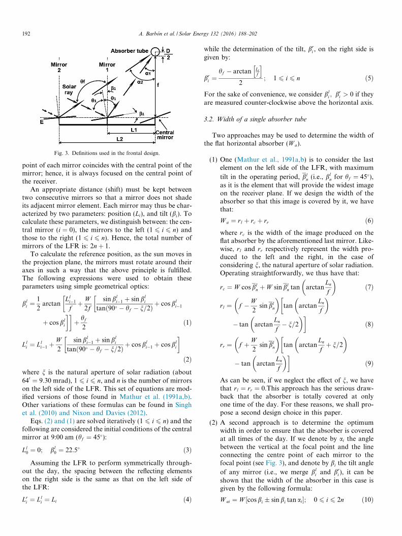
Fig. 3. Definitions used in the frontal design.

192 A. Barbon et al. / Solar Energy 132 (2016) 188–202

point of each mirror coincides with the central point of themirror; hence, it is always focused on the central point ofthe receiver.

An appropriate distance (shift) must be kept betweentwo consecutive mirrors so that a mirror does not shadeits adjacent mirror element. Each mirror may thus be char-acterized by two parameters: position (Li), and tilt (bi). Tocalculate these parameters, we distinguish between: the cen-tral mirror (i ¼ 0), the mirrors to the left (1 6 i 6 n) andthose to the right (1 6 i 6 n). Hence, the total number ofmirrors of the LFR is: 2nþ 1.

To calculate the reference position, as the sun moves inthe projection plane, the mirrors must rotate around theiraxes in such a way that the above principle is fulfilled.The following expressions were used to obtain theseparameters using simple geometrical optics:

bli ¼

1

2arctan

Lli�1

fþ W2f

sin bli�1 þ sin bl

i

tanð90� � hf � n=2Þ þ cos bli�1

��þ cos bl

i

��þ hf

2ð1Þ

Lli ¼ Ll

i�1 þW2

sin bli�1 þ sin bl

i

tanð90� � hf � n=2Þ þ cos bli�1 þ cos bl

i

� �ð2Þ

where n is the natural aperture of solar radiation (about640 ¼ 9:30 mrad), 1 6 i 6 n, and n is the number of mirrorson the left side of the LFR. This set of equations are mod-ified versions of those found in Mathur et al. (1991a,b).Other variations of these formulas can be found in Singhet al. (2010) and Nixon and Davies (2012).

Eqs. (2) and (1) are solved iteratively (1 6 i 6 n) and thefollowing are considered the initial conditions of the centralmirror at 9:00 am (hf ¼ 45�):

Ll0 ¼ 0; bl

0 ¼ 22:5� ð3ÞAssuming the LFR to perform symmetrically through-

out the day, the spacing between the reflecting elementson the right side is the same as that on the left side ofthe LFR:

Lri ¼ Ll

i ¼ Li ð4Þ

while the determination of the tilt, bri , on the right side is

given by:

bri ¼

hf � arctan Lif

h i2

; 1 6 i 6 n ð5Þ

For the sake of convenience, we consider bli ; br

i > 0 if theyare measured counter-clockwise above the horizontal axis.

3.2. Width of a single absorber tube

Two approaches may be used to determine the width ofthe flat horizontal absorber (W a).

(1) One (Mathur et al., 1991a,b) is to consider the lastelement on the left side of the LFR, with maximum

tilt in the operating period, bln (i.e., bl

n for hf ¼ 45�),as it is the element that will provide the widest imageon the receiver plane. If we design the width of theabsorber so that this image is covered by it, we havethat:

W a ¼ rl þ rc þ rr ð6Þ

where rc is the width of the image produced on theflat absorber by the aforementioned last mirror. Like-wise, rl and rr respectively represent the width pro-duced to the left and the right, in the case ofconsidering n, the natural aperture of solar radiation.Operating straightforwardly, we thus have that:

rc ¼ W cos bln þ W sin bl

n tan arctanLn

f

� �ð7Þ

rl ¼ f � W2

sin bln

� �tan arctan

Ln

f

� ��� tan arctan

Ln

f� n=2

� ��ð8Þ

rr ¼ f þ W2

sin bln

� �tan arctan

Ln

fþ n=2

� ��� tan arctan

Ln

f

� ��ð9Þ

As can be seen, if we neglect the effect of n, we havethat rl ¼ rr ¼ 0.This approach has the serious draw-back that the absorber is totally covered at onlyone time of the day. For these reasons, we shall pro-pose a second design choice in this paper.

(2) A second approach is to determine the optimumwidth in order to ensure that the absorber is coveredat all times of the day. If we denote by ai the anglebetween the vertical at the focal point and the lineconnecting the centre point of each mirror to thefocal point (see Fig. 3), and denote by bi the tilt angle

of any mirror (i.e., we merge bli and br

i ), it can beshown that the width of the absorber in this case isgiven by the following formula:

W ai ¼ W cos bi � sin bi tan ai½ �; 0 6 i 6 2n ð10Þ

Fig. 4. Cylindrical absorber.

A. Barbon et al. / Solar Energy 132 (2016) 188–202 193

which, as can be seen, depends on each mirror, andwhere the sign � must be adopted according to thefollowing criteria: � for the left side, and þ for theright side.In this study, we have considered the latter option tobe far better; although there are times when the sun’srays fall outside the single absorber tube, it is pre-cisely there where the design of the secondary reflec-tor must play a decisive role. The design value thatwe shall consider is:

W �a ¼ min

06i62nW ai ð11Þ

a value which means that the entire absorber willalways be illuminated. We shall see the resultsobtained in the different simulations in Section 6.The reader will have noticed that, for the sake of sim-plicity, up until now we have considered a flat absor-ber. However, our design will use cylindrical tubes,whose diameter (D) will be one of the key factors inthe design. For this reason and to conclude the fron-tal study, let us now see the equivalent formulas to(10) to use in the case of a cylindrical absorber.If we denote by Lai the length of the circumferenceilluminated on the absorber by the i-th mirror (seeFig. 4), it holds that:

Lai ¼pD2

if W ai cos ai > D

D arcsin W aiD

� �if W ai cos ai 6 D

(ð12Þ

for 0 6 i 6 2n. We must bear in mind that the realvalue of D must be chosen from among the availablestandard values for the tubes. Thus, the most reason-able choice for the frontal design is to work with W �

a

to compute CR (see (36)) and, once the design is cho-sen and the value of W �

a is fixed, we can choose the Dof the tube that best fits the conditions (12), i.e., theone which verifies in most cases W ai cos ai P D.A final modification also needs to be made in theabove formulas. This simply involves changing thefocal distance, f, in all the above formulas in whichit appears by:

f 0 ¼ f þ D2

ð13Þ

to take into account the radius of the absorber tube.

3.3. Frontal cosine factor

Finally, it is worth noting that the radiation incident isperpendicular to each mirror-reflector in the frontal planeview once a day. In all other cases, the total radiation onthe LFR is directly proportional to the cosine of the anglebetween the normal to the mirror and the angle of inci-dence of the sun (hi). This factor can be deduced; its valuebeing:

cos hi ¼ cosjhf j þ ai

2; 0 6 i 6 2n ð14Þ

As can be seen in (14), this factor has a value for each mir-ror depending on the position of the sun. We shall subse-quently see the influence of this factor on the actualradiation that is harnessed.

It should be noted that there is another cosine factor toanalyse, namely the one produced when the solar radiationreaches the absorber. In the case of the frontal study, it isstraightforward to deduce that the following holds:

cos hai ¼ 1; 0 6 i 6 2n ð15Þ

as the surface of the incident ray is equal to the surface illu-minated by the ray.

3.4. Reflection of non-parallel rays

The preceding study is based on the incident light raysbeing parallel. Actually, this is not true: because of thefinite angular size of the sun’s disc, the sun’s rays reachingthe absorber tube are not parallel. Therefore, this consider-ation affects the focus width and hence the design of thesecondary reflector. It specifically affects the calculationof the aperture of the secondary reflector. As already sta-ted, however, this question is not addressed in this paper.

Let us consider the angular diameter of the sun’s disc,n ’ 9:3 mrad (see Stine and Geyer, 2015). Fig. 5 shows thattaking this parameter into consideration means that thefocus width, W ai, varies with respect to the value calculatedin (10). Obviously, this change also affects Lai. The illumi-nated area is now increased in two values that we shall calld 0i and d 00

i . Their values affect the aperture of the secondaryreflector, more than the diameter of the absorbing tube.

The aim is thus to calculate the length of the lower leg ofthe striped, right-angled triangles in Fig. 5. To determinethese distances, we straightforwardly have that:

Fig. 6. Definitions used in the lateral design.

194 A. Barbon et al. / Solar Energy 132 (2016) 188–202

H 0i ¼ Li�W

2½cosðbiÞ� sinðbiÞ tanðaiÞ�

� �2

þ f þD2

� �2" #1=2

;

06 i6 2n ð16Þ

H 00i ¼ LiþW

2½cosðbiÞ� sinðbiÞ tanðaiÞ�

� �2

þ f þD2

� �2" #1=2

;

06 i6 2n ð17ÞThe sign � must be adopted, once again, according to thefollowing criteria: � for the left side, and þ for the rightside. Hence, the distances to determine are:

d 0i ¼ H 0

i tann2

ð18Þ

d 00i ¼ H 00

i tann2

ð19Þ

These values of d 0i and d 00

i are then added to the previouslycalculated value of W ai. Their influence is thus limited tothe frontal study (see Section 6.2); they barely affect the lat-eral study subsequently presented in Section 6.3.

4. Lateral design

In what follows, we shall perform the lateral study of theLFR. The aim is to compute the optimal relative disposi-tion between the field of primary reflectors and the singleabsorber tube.

In large-scale LFRs, this study is not usually conductedfor two reasons. First of all, the size of the absorber doesnot permit any configuration to modify its position. Sec-ond, the influence of the lateral position can be consideredirrelevant in % terms with respect to the total length of thesingle absorber tube. However, in smaller-sized LFRs, likethose analysed in this paper, this is a fundamental study, aswe shall subsequently show. In Fig. 6, we describe the nota-tion. We need only take into account the central mirror forthis study. Apart from the new variables (which we do notdefine for the sake of brevity), as before k is the latitude, hzis the zenithal solar angle (with hz ¼ hl), f is the distance to

Fig. 5. Reflection of non-parallel rays.

the absorber and d is the declination. LM represents thelength of the mirrors.

Fig. 6 shows the most general configuration possible(C1). All the particular cases can be deduced from the for-mulas obtained for this configuration. The following rela-tions between the angles can be verified:

hL ¼ hz � kþ d ð20Þl ¼ �hz þ 2k� 2d ð21Þand also those between the distances:

y1 ¼ f þ LM

2sinðk� dÞ ð22Þ

y2 ¼ x0 þ LM

2cosðk� dÞ

� �tanðk� dÞ ð23Þ

y3 ¼ f � LM

2sinðk� dÞ ð24Þ

y4 ¼LM

2cosðk� dÞ � xf

� �tanðk� dÞ ð25Þ

xi ¼ yi tan l; i ¼ 1; 2; 3; 4 ð26ÞFrom the above, after some computations, we have that:

x0 ¼ x1 � x2 ¼ f tan l cosðk� dÞcosðk� dÞ þ sinðk� dÞ tan l ð27Þ

and

xf ¼ x3 þ x4 ¼ f tan l cosðk� dÞcosðk� dÞ þ sinðk� dÞ tan l ð28Þ

Thus, x0 ¼ xf . We also need to consider two lateral cosinefactors: one at the mirror and another one at the singleabsorber tube, which measure the deviation of the incidentsolar ray from the normal with respect to each of the sur-faces. For example, in the configuration shown in Fig. 6,both would be equal to:

cos hL ¼ cos hz � kþ dð Þ ð29Þwhich can be seen just by using (20). We proceed to show12 different configurations for the relative position betweenthe field of primary mirrors and the absorber. Table 1shows whether the absorber (A) is fixed (F) or movable

A. Barbon et al. / Solar Energy 132 (2016) 188–202 195

(M), the inclination angle of the single absorber tube (tA)and the incidence angle at the single absorber tube (aA).The same data is given for the primary reflectors (Mi).

Position C1 is inspired by a setting similar to that used inthe so-called single axis polar solar tracker. These followersrotate on an axis oriented in the NS direction at an axialinclination equal to the latitude k of the place, sometimescorrected by means of the declination, d. Thus, the rotationaxis of the system is parallel to the axis of the Earth. Singleaxis polar solar trackers reach yields of over 96% comparedto systems with two axes. This is why we consider this asthe basic configuration. In C1, both A and Mi are movable,but they keep their inclination, k� d, throughout the dayand only move from day to day.

Starting at C1 and maintaining the same configurationof mirrors, we performed the variations C2, C3, C4 andC5 employing different fixed inclinations for the absorber.The angle f ¼ 21:47� appears in position C4. This is definedas the angle hz for day n ¼ 195 and for solar time T S ¼ 12.We chose these values because they correspond to the dayand time of maximum radiation in the whole year. In these5 positions, the following holds:

hL ¼ hz � kþ d; l ¼ �hz þ 2k� 2d ð30ÞFor position C6, we also consider A and Mi as movable.

In this case, however, they do move throughout the day,

because the chosen angle aA ¼ aMi ¼ hz2

� �depends on

the solar time. With this angle, the following holds:

hL ¼ hz2; l ¼ 0 ð31Þ

and its value is chosen so that the rays exit Mi perpendic-ular to the floor. As we shall see in more detail in Section 6,we thus have that the position of A is just above Mi, pre-venting displacements which are highly detrimental to thedesign. As before, and starting at C6, we perform variationsmaintaining A fixed and employing different inclinations.Observe, for example, that in C9, the cosine of the angleover A is cos 0 ¼ 1.

Positions C10 and C11 are inspired by the more classicaldesigns of immovable LFRs. In these, the following holds:

Table 1Configurations.

A tA aA Mi tMi aMi

C1 M k� d hL M k� d hLC2 F k d M k� d hLC3 F k=2 dþ k=2 M k� d hLC4 F f dþ k� f M k� d hLC5 F 0� l M k� d hLC6 M hz=2 hz=2 M hz=2 hz=2C7 F k k M hz=2 hz=2C8 F f f M hz=2 hz=2C9 F 0� 0� M hz=2 hz=2C10 F k hz � k F k hz � kC11 F 0� �hz þ 2k F k hz � kC12 F 0� hz F 0� hz

hL ¼ hz � k; l ¼ �hz þ 2k ð32ÞFinally, position C12 is the most common in large-scaleLFRs, with A and Mi being horizontal and fixed. All theseconfigurations shall be tested and we need parameters thatallow us to assess their goodness from different points ofview. This is what we shall do in the next section.

5. Efficiency of a LFR

To perform a suitable comparative analysis, we mustdefine the relevant parameters to assess each of the sug-gested configurations. Many types of efficiency are pre-sented in the literature: energy efficiency or opticalefficiency, as in for example (see Montes et al., 2014):

genergyð%Þ ¼ Eir

DNI � Apm100 ð33Þ

gopticalð%Þ ¼ qmRaysincident receiver

Raystotal100 ð34Þ

where qm represents the reflectivity of the primary mirrors,Eir (W) is the incident energy on the receiver, DNI ðW=m2Þis the Direct Normal Irradiance, and Apm ðm2Þ the surfacearea of the primary mirrors. As our study does not includeeither thermal or energetic aspects, we must accordinglyfind geometric parameters which characterize both designs.

Different equations are used in the literature (see, forexample, Morin et al., 2012; Elmaanaoui and Saifaoui,2014; Cau and Cocco, 2014) to determine the powerabsorbed by the absorber tube of an LFR. All of themare made up of the same terms, in general. The total powerabsorbed from the solar field is thus usually calculatedfrom:

Q ¼ DNI � gopt;0 � xfield � CI � IAM � Am � gendloss ð35Þwhere the parameters are: DNI, the Direct Normal Irradi-ance (Nikitidou et al., 2014), which is the direct irradiancereceived by a surface that is always held normal to theincoming sun’s rays, gopt;0 is the optical efficiency of the

LFR for normal incidence rays to the horizontal ðh ¼ 0Þ(Nixon et al., 2013), xfield is the availability of the solarfield; CI is the cleanliness factor, IAM is the incidence anglemodifier (Sallaberrya et al., 2014), and describes the varia-tion in optical performances of the LFR for varying inci-dence angles of rays, Am is the total area of the LFR, andgendloss is the end loss efficiency (Morin et al., 2012), whichdescribes the length of the receiver which is not illuminatedby the reflected rays.

In Eq. (35), the IAM contains the variation in the opticalperformance of a LFR for varying ray incidence angles.However, whereas the IAM generally only considers thefrontal design for the case of a large-scale LFR, we con-sider simultaneously the frontal and the lateral design. Insmall-scale LFRs, the influence of the lateral design is veryimportant, as we shall see in Section 6. Besides, as this fac-tor is different for each mirror, it will henceforth bedenoted as R0

i (see (52)).

196 A. Barbon et al. / Solar Energy 132 (2016) 188–202

5.1. Frontal design

One of the most important and simplest ways of charac-terizing LFRs is via their concentration ratio (CR) or fillingfactor (Montes et al., 2014), defined as:

CR ¼ Apm

Aabsð36Þ

Aabs ðm2Þ being the area of the single absorber tube andApm ðm2Þ, the surface area of the primary reflectors, givenby:

Apm ¼ ð2nþ 1Þ � W � LM ð37ÞAabs ¼ Lai � Labs ð38Þwhere we shall assume, for the frontal design, that thelength of the absorber is equal to that of the mirrors:

Labs ¼ LM ð39ÞThis quantity serves as a reference for the increase in the

density of radiating flux, given that, in a LFR, the rays areconcentrated on a much smaller area than that of the mir-rors. However, the incidence angle of the sun is not normalto all the mirrors, so that the true area of the mirrors is notApm, but in fact it is necessary to compute the projection ofeach of the mirrors with respect to the incidence of the raysof the sun. This is why some authors (Singh et al., 2010)also use the real concentration ratio (CRr) defined as:

CRr ¼ Apm r

Aabs¼

P2ni¼0W � LM � cos hi

Aabsð40Þ

obtained by summing the concentration contribution of the2nþ 1 mirrors. In this paper, the assessment of each of theconfigurations of the frontal design will be carried outusing only the parameter (36). The reason for not using(40) is its dependence on the time of the day (see (14)),which complicates the study unnecessarily.

5.2. Lateral design

In order to analyse the lateral design, however, giventhat the width of the single absorber tube is irrelevant,other parameters must be taken into consideration toachieve a proper assessment of the design. Undoubtedly,due to its influence on the quantity of incident radiation,the most important parameter is the true length of theabsorber that is illuminated at each time. In the previoussection on the frontal design, for the sake of simplicitywe assumed that Labs ¼ LM . However, we shall see that thisis not always the most efficient setting.

Moreover, if the absorber is placed such that its end-points coincide with those of the mirrors, it will have ano illuminated area in most configurations. This is whywe shall also have to take into account the relative lateralposition of the absorber with respect to the primary mir-rors. This factor is important not only to optimize the usedradiation, but also from the point of view of the design: if

the illuminated area of the absorber is shifted too far fromthe vertical of the field of primary reflectors, it may give riseto technically unfeasible configurations.

Thus, we define the left illuminated length of the absor-

ber, lla, as:

lla ¼x0 þ LM

2cosðk� dÞ

cosðk� dÞ ð41Þ

and the right illuminated length of the absorber, lra, as:

lra ¼LM2cosðk� dÞ � xfcosðk� dÞ ð42Þ

both measured from the vertical to the midpoint of the cen-tral mirror (see Fig. 5). With these values, we can then com-pute the total illuminated length:

lTa ¼ lla þ lra ð43Þ

and, from this, we can define a new parameter, the lengthratio (LR):

LR ¼ lTaLM

ð44Þ

which shall allow us to compare the different configura-

tions. Moreover, lla and lra will also allow us to place A ver-sus Mi in an unequivocal way. We define the deviation withrespect to the vertical De as:

De ¼ lla � lra ð45Þwhere the sign of De indicates whether it is to the S (þ) orthe N (�). Note that this concept has not been consideredin such detail till now by any author. The reader can find ashort outline of this type of study in Pu and Xia (2011).

5.3. Joint design

In the previous paragraphs, we have seen parameterswhich allow us to assess the efficiency of the frontal: (36)and (40) and lateral design: (44) and (45) separately. Weshall complete this section by presenting a decidedly funda-mental aspect: the combination of both studies, the frontaland the lateral design. Both parameters may be combinedin a single one as follows:

P ¼ x1CRþ x2LRþ x3De ð46ÞThis would have the drawback, however, of having to

choose the weight functions, xi ði ¼ 1; 2; 3Þ, in such away that is not detrimental to one study versus the other.This is why we consider the most representative parameterto be the resultant, Ri, of the incident radiation, R (withjRj ¼ 1). Looking at Fig. 2 again, it can be seen that R

has two components: the lateral one, Rl, common to allthe mirrors, and the frontal one, Rfi, which depends oneach mirror. It is straightforward to prove that they satisfythe following equalities:

A. Barbon et al. / Solar Energy 132 (2016) 188–202 197

Rl ¼ cos cS cos aScos cS

¼ cos aS ð47Þ

Rfi ¼ cos cS sin aSsin hf

; 0 6 i 6 2n ð48Þ

The sum of these two concurrent vectors is:

R2i ¼ R2

l þ R2fi þ 2RlRfi cos dRlRfi ; 0 6 i 6 2n ð49Þ

If we now take into account the terms introduced by theincidence cosines at each mirror, both the lateral (hL) andthe frontal cosine (hi), we have that:

R0l ¼ Rl cos hL ð50Þ

R0fi ¼ Rfi cos hi; 0 6 i 6 2n ð51Þ

from which the resultant, R0i (0 6 i 6 2n) is:

R0i ¼ R02

l þ R02fi þ 2R0

lR0fi cos

dR0lR

0fi

h i1=2ð52Þ

simply by assuming that the cos dR0lR

0fi is equal at the entry

and exit on each mirror.

Remark. As they ignore the lateral study, most authors usethe simplified formula:

R0i ’ Rsim

i ¼ R cos hi; 0 6 i 6 2n ð53ÞIn the following section, we shall see how this simplifica-

tion leads to important design errors in some cases.

6. Numerical simulation

Several ray tracing programs have been reported in thebibliography. In Mills and Morrison (2000), a ray tracemodel was used in a radiation and thermal model devel-oped in TRNSYS. The model generates optical collectionmaps in terms of transverse and longitudinal incidenceangles. In Grena and Tarquini (2011), a ray-tracing pro-gram was written using C++ to predict the optical perfor-mance of the system. A software application calledTracePro, based on the Monte Carlo ray tracing (MCRT)method, is very known (Xie et al., 2011b; Lin et al., 2013,2014). TracePro is used to simulate the scattering anddiffraction of light. In Monte Carlo ray tracing, scatteringand diffraction are treated as random processes. The readeris referred to Garcia et al. (2008), for more information onprograms of this kind, which provides a review of the mainfeatures of six codes for concentrated solar flux calculation(UHC, DELSOL, HFLCAL, MIRVAL, FIAT LUX andSOLTRACE).

In this study, however, we decided to develop a newcode, implemented in Mathematica� to estimate the opticalefficiency of the LFR system presented in this paper.

6.1. Programming

Once both the lateral and frontal designs of the LFRhave been chosen, hf and hz must be expressed as functions

of the daytime angle, x, which in turn must be expressed asa function of the legal time, T L, in order to program theProgrammable Logic Control (PLC). It is also well-known that the normal vectors to mirrors at their centralpoints are not parallel to one another. However, the anglemade by the normal vectors for two different sun positionsis the same for all mirrors. This fact permits rotating all themirrors of the LFR through the same angle. We accord-ingly considered two possibilities for the programming:

(i) Always rotating all the mirrors through the sameangle, but calibrating the time of the rotation as afunction of the day of the year.

(ii) Or rotating the mirrors through an angle that varieswith the day of the year, but the same for all the mir-rors, at a specified daytime.

In this study, we have chosen the second option, the rea-son being none other than the choice of a stepper motor.This is a special type of electric motor that moves in incre-ments or steps. The size of the increment is measured indegrees. We shall use increments of 1:8� and, as the motorincludes a gear ratio of 100 : 1, which means we can obtainan angle of 0:018� per step.

For the computations of the design, following Spencer(1971) and Duffie and Beckman (2006), we shall considereach day of the year, nd , one by one, which by means of:

C ¼ ðnd � 1Þ 2p365

ð54Þ

fixes the daily angle, C, and, as a function of this, by meansof the following equations:

ET ¼ 229:18½0:0000075þ 0:001868 cosC� 0:032077 sinC

� 0:014615 cos 2C� 0:04089 sin 2C� ð55Þd ¼ 0:006918� 0:399912 cosCþ 0:070257 sinC

� 0:006758 cos 2Cþ 0:000907 sin 2C� 0:002697 cos 3C

þ 0:001480 sin 3C ð56Þthe declination, d, and the time equation, ET, both constantfor each day. Furthermore, the latitude, k, and the longitude,L0, are fixed for each position of the LFR. Simply taking intoaccount the relation of aS and cS with x, given by:

cS ¼ arcsin½sin d sin kþ cos d cos k cosx� ð57Þ

aS ¼ signðxÞ � arccos sin cS sin k� sin dcos cS cos k

� �ð58Þ

and the relation between x and T L, given by:

T L ¼ 12þ x� 1

15ðL0 � LUTCÞ � ET

60þ AH ð59Þ

and by means of elementary computations and substitutingin:

hf ¼ arctansin cStan aS

� �ð60Þ

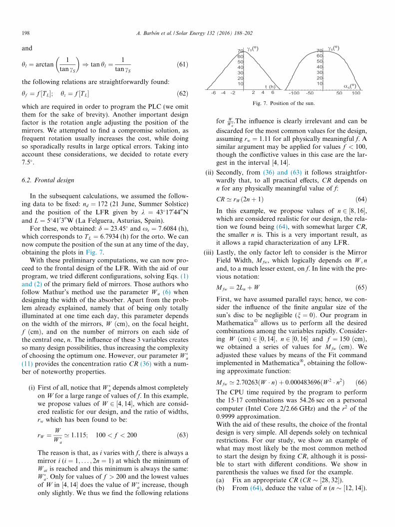
Fig. 7. Position of the sun.

198 A. Barbon et al. / Solar Energy 132 (2016) 188–202

and

hl ¼ arctan1

tan cS

� �) tan hl ¼ 1

tan cSð61Þ

the following relations are straightforwardly found:

hf ¼ f ½T L�; hz ¼ f ½T L� ð62Þwhich are required in order to program the PLC (we omitthem for the sake of brevity). Another important designfactor is the rotation angle adjusting the position of themirrors. We attempted to find a compromise solution, asfrequent rotation usually increases the cost, while doingso sporadically results in large optical errors. Taking intoaccount these considerations, we decided to rotate every7:5�.

6.2. Frontal design

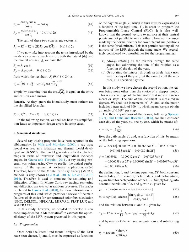
In the subsequent calculations, we assumed the follow-ing data to be fixed: nd ¼ 172 (21 June, Summer Solstice)and the position of the LFR given by k ¼ 43�1704400Nand L ¼ 5�410300W (La Felguera, Asturias, Spain).

For these, we obtained: d ¼ 23:45� and xs ¼ 7:6084 (h),which corresponds to T L ¼ 6:7934 (h) for the orto. We cannow compute the position of the sun at any time of the day,obtaining the plots in Fig. 7.

With these preliminary computations, we can now pro-ceed to the frontal design of the LFR. With the aid of ourprogram, we tried different configurations, solving Eqs. (1)and (2) of the primary field of mirrors. Those authors whofollow Mathur’s method use the parameter W a (6) whendesigning the width of the absorber. Apart from the prob-lem already explained, namely that of being only totallyilluminated at one time each day, this parameter dependson the width of the mirrors, W ðcmÞ, on the focal height,f ðcmÞ, and on the number of mirrors on each side ofthe central one, n. The influence of these 3 variables createsso many design possibilities, thus increasing the complexityof choosing the optimum one. However, our parameter W �

a

(11) provides the concentration ratio CR (36) with a num-ber of noteworthy properties.

(i) First of all, notice that W �a depends almost completely

on W for a large range of values of f. In this example,we propose values of W 2 ½4; 14�, which are consid-ered realistic for our design, and the ratio of widths,rw which has been found to be:

rW ¼ WW �

a

’ 1:115; 100 < f < 200 ð63Þ

The reason is that, as i varies with f, there is always amirror i (i ¼ 1; . . . ; 2n ¼ 1) at which the minimum ofW ai is reached and this minimum is always the same:W �

a. Only for values of f > 200 and the lowest valuesof W in ½4; 14� does the value of W �

a increase, thoughonly slightly. We thus we find the following relations

for WW �

a.The influence is clearly irrelevant and can be

discarded for the most common values for the design,assuming rw ¼ 1:11 for all physically meaningful f. Asimilar argument may be applied for values f < 100,though the conflictive values in this case are the lar-gest in the interval ½4; 14�.

(ii) Secondly, from (36) and (63) it follows straightfor-wardly that, to all practical effects, CR depends onn for any physically meaningful value of f:

CR ’ rW ð2nþ 1Þ ð64Þ

In this example, we propose values of n 2 ½8; 16�,which are considered realistic for our design, the rela-tion we found being (64), with somewhat larger CR,the smaller n is. This is a very important result, asit allows a rapid characterization of any LFR.

(iii) Lastly, the only factor left to consider is the MirrorField Width, Mfw, which logically depends on W ; nand, to a much lesser extent, on f. In line with the pre-vious notation:

Mfw ¼ 2Ln þ W ð65Þ

First, we have assumed parallel rays; hence, we con-sider the influence of the finite angular size of thesun’s disc to be negligible (n ¼ 0Þ. Our program inMathematica� allows us to perform all the desiredcombinations among the variables rapidly. Consider-ing W ðcmÞ 2 ½0; 14�; n 2 ½0; 16� and f ¼ 150 ðcmÞ,we obtained a series of values for Mfw ðcmÞ. Weadjusted these values by means of the Fit commandimplemented in Mathematica�, obtaining the follow-ing approximate function:

Mfw ’ 2:70263ðW � nÞ þ 0:000483696ðW 2 � n2Þ ð66ÞThe CPU time required by the program to performthe 15�17 combinations was 54:26 sec on a personalcomputer (Intel Core 2/2:66 GHz) and the r2 of the0:9999 approximation.With the aid of these results, the choice of the frontaldesign is very simple. All depends solely on technicalrestrictions. For our study, we show an example ofwhat may most likely be the most common methodto start the design by fixing CR, although it is possi-ble to start with different conditions. We show inparenthesis the values we fixed for the example.(a) Fix an appropriate CR (CR � ½28; 32�).(b) From (64), deduce the value of n (n � ½12; 14�).

A. Barbon et al. / Solar Energy 132 (2016) 188–202 199

(c) Fix the maxMfw available ðmax Mfw � 200Þ.(d) From (66), compute W (W � ½5; 6�).

Fig. 8. lTa ; lla and lra of configuration C1.

Fig. 9. lTa ; lla and lra of configuration C6.

Table 2Relation W =W �

a.

W f

250 300 350 400

4 1.109 1.106 1.104 1.1015 1.113 1.110 1.107 1.1056 1.115 1.113 1.110 1.1087 1.115 1.114 1.113 1.111

Table 3Influence of nd on De.

max lla min lla max lra min lla

C1 356 172 172 356C6 cte cte cte cteC12 172 356 356 172

Finally, we determined the size of the system, with 25mirrors (n ¼ 12), W ¼ 6 (cm) width, with the plane of theabsorber placed at f ¼ 150 (cm). For this setup,CR ¼ 27:88; Mfw ¼ 196:36 and W �

a ¼ 5:37. The reflectivesurfaces are commercial grade, 3 (mm) thick andLM ¼ 200 (cm) long. As regards the absorber tube, wechose a diameter D ¼ 5:34 (cm) for the reason that, amongthose available, it is the one which best fits the followingcondition: W ai cos ai P D.

Finally, we verified the negligible influence on the fron-tal design of the finite angular size of the sun’s disc, n. If theabove calculations are repeated with n ¼ 9:3 mrad, the fol-lowing approximate function is obtained:

Mfw ’ 2:71112ðW � nÞ þ 0:000503639ðW 2 � n2Þ ð67ÞAs can be seen, the dimensions are now slightly greater

than in the previous case. The reason for this is that consid-ering the rays to be non-parallel by including n, the separa-tion between mirrors must be somewhat greater in order toavoid the effects of blocking and shading. Nonetheless, thedifference is very small. The greatest relative error betweenthe two approaches is 0.45%, the value obtained in theextreme case of W ¼ 14 (cm), and n ¼ 16.

6.3. Lateral design

We now present the results obtained for the lateraldesign. Of all the previous configurations, we start byshowing the cases C1, C6, C12 (configuration C10 is notanalysed because it is very similar to C12). These 3 caseswere chosen due to being the most relevant ones. The basecase is C1, inspired by the single axis polar solar tracker,with A and Mi fixed throughout the day, though adjustablefrom day to day; case C6 has A and Mi varying throughoutthe day; case C12, the most common in large-scale LFRs,has A and Mi horizontal and fixed.

Moreover, all of these cases verify that the angles of theabsorber and the mirrors are equal (from the lateral point

of view): aA = aMi. Hence, we have that lTa ¼ 200 (cm) forall cases and hence LR ¼ 1. What does vary from a config-uration to another is the shift relative to the vertical De.

In Fig. 8, we show lTa ; lla and lra for C1. Analysing the

influence of T S, we see that lla (resp. lra) increases (resp.decreases) from T S = 7:00 h (or 17:00 h by symmetry) to12:00 h, regardless of the day, nd . The influence of nd ,regardless of T S , can be seen in Table 3.

In Fig. 9, we show how in C6, both lla and lra remain con-

stant regardless of the day or time lla ¼ lra ¼ 100 (cm).

In case C12, as in C1, lla (resp. lra) increases (resp.decreases) from T S = 7:00 h (or 17:00 h by symmetry) to12:00 h, irrespective of the day, nd , though now the influ-ence of nd (see Table 2) is the opposite. Recall that

nd ¼ 356 corresponds to the Winter solstice and nd ¼ 172corresponds to the Summer solstice.

The effect of De is perceived more clearly in Figs. 10 and11, where it is apparent that in order for the absorber to beilluminated, at times it needs to be shifted some metres.Thus, if we only analyse the factors LR and De among theseconfigurations (the three with LR ¼ 1), C6 is undoubtedlythe best one from the constructive point of view.

Apart from the two parameters LR and De already stud-ied, it is also of interest to assess the different configura-tions from the point of view of the lateral angle ofincidence on the mirror: cos hL, due to its effect on the totalradiation, R0

i. This factor is shown in Fig. 12 for C1, C6 andC12.

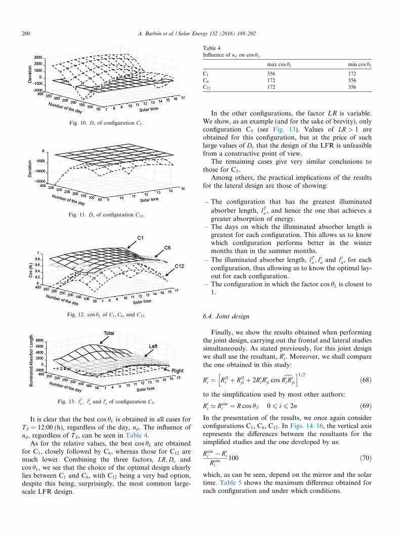
Fig. 10. De of configuration C1.

Fig. 11. De of configuration C12.

Fig. 12. cos hL of C1;C6, and C12.

Table 4Influence of nd on cos hL.

max cos hL min cos hL

C1 356 172C6 172 356C12 172 356

Fig. 13. lTa ; lla and lra of configuration C5.

200 A. Barbon et al. / Solar Energy 132 (2016) 188–202

It is clear that the best cos hL is obtained in all cases forT S = 12:00 (h), regardless of the day, nd . The influence ofnd , regardless of T S , can be seen in Table 4.

As for the relative values, the best cos hL are obtainedfor C1, closely followed by C6, whereas those for C12 aremuch lower. Combining the three factors, LR;De andcos hL, we see that the choice of the optimal design clearlylies between C1 and C6, with C12 being a very bad option,despite this being, surprisingly, the most common large-scale LFR design.

In the other configurations, the factor LR is variable.We show, as an example (and for the sake of brevity), onlyconfiguration C5 (see Fig. 13). Values of LR > 1 areobtained for this configuration, but at the price of suchlarge values of De that the design of the LFR is unfeasiblefrom a constructive point of view.

The remaining cases give very similar conclusions tothose for C5.

Among others, the practical implications of the resultsfor the lateral design are those of showing:

– The configuration that has the greatest illuminated

absorber length, lTa , and hence the one that achieves agreater absorption of energy.

– The days on which the illuminated absorber length isgreatest for each configuration. This allows us to knowwhich configuration performs better in the wintermonths than in the summer months.

– The illuminated absorber length, lTa ; lra and lla, for each

configuration, thus allowing us to know the optimal lay-out for each configuration.

– The configuration in which the factor cos hL is closest to1.

6.4. Joint design

Finally, we show the results obtained when performingthe joint design, carrying out the frontal and lateral studiessimultaneously. As stated previously, for this joint designwe shall use the resultant, R0

l. Moreover, we shall comparethe one obtained in this study:

R0i ¼ R02

l þ R02fi þ 2R0

lR0fi cos

dR0lR

0fi

h i1=2ð68Þ

to the simplification used by most other authors:

R0i ’ Rsim

i ¼ R cos hi; 0 6 i 6 2n ð69ÞIn the presentation of the results, we once again considerconfigurations C1, C6, C12. In Figs. 14–16, the vertical axisrepresents the differences between the resultants for thesimplified studies and the one developed by us:

Rsimi � R0

i

Rsimi

100 ð70Þ

which, as can be seen, depend on the mirror and the solartime. Table 5 shows the maximum difference obtained foreach configuration and under which conditions.

Fig. 14. Influence of the lateral design on C1.

Fig. 15. Influence of the lateral design on C6.

Fig. 16. Influence of the lateral design on C12.

Table 5Influence of the lateral study on the resultant.

max% nd T S Mirror no.

C1 �38.69 356 9:00 (15:00) 12 Left (Right)C6 �17.86 356 8:00 (16:00) 12 Left (Right)C12 +60.48 356 12:00 Central

A. Barbon et al. / Solar Energy 132 (2016) 188–202 201

We can see how the classical studies, carried out forlarge-scale LFRs and which ignore the lateral study, areinadequate for small-scale LFRs, as very large errors canoccur.

7. Conclusions

LFR technologies constitute a hot research topic. Anumber of different LFR systems are currently being devel-oped by different companies, such as Novatec Solar (Ger-many), Areva Solar (France/USA), MAN/Solar PowerGroup (Germany), Industrial Solar (Germany), Fera(Italy) and CNIM (France). The LFR has several advan-tages: it is very useful for medium-temperature range appli-cations (between 100 and 250 �C); it is fabricated with

narrow flat mirrors, materials readily and cheaply availableon the market; and the planar configuration and the air gapbetween the adjacent mirrors result in low wind loading onthe structure. The first commercial plants are already inservice and the previous literature contains several LFRdesigns.

This paper focuses on an optical andmathematical study,without addressing thermal or economic aspects. The designof a LFR is usually analysed considering a horizontal singleabsorber tube. In this paper, however, various configura-tions have been analysed taking into account the lateralview. This study is fundamental when the aim is to obtainthe optimal design of a LFR for the Household Sector.The following energy consumptions in households can beidentified: space heating, water heating, cooking, space cool-ing, lighting and electrical appliances. Thermal energy usescorrespond to 85% of all household consumption.

Our study has allowed us to show the importance of thislateral design, which, in combination with the frontaldesign, leads to the optimal solution from the optical pointof view. While the frontal design focuses on calculating thenumber, width and optimal separation of the primary mir-rors, as well as the focal height, the lateral design focuseson the relative position between the single absorber tubeand the primary reflector. The best design combinationhas been determined on the basis of new efficiency param-eters introduced for the first time in this paper. Further-more, some of the 12 configurations we present meanthat our LFR is actually a hybrid between types I and II,as they allow movement of the individual reflector-rowsand that of the reflector-receiver system.

As far as future perspectives are concerned, the subjectof the design of the secondary reflector concentrator stillremains open. The single absorber tube device plays a veryimportant role in the harnessing of solar energy and thesecondary reflector geometry also requires detailed study.It would also be interesting to continue this line of researchvia the study of thermal behaviour. It should also be notedthat, at the time for writing this paper (April 2015), a pro-totype is being built at the CIFP-Mantenimiento y Servi-cios a la Produccion, in La Felguera, Asturias, Spain,that will enable a comparison with theoretical results.

Acknowledgements

We wish to thank M.F. Fanjul, director of the CIFP inLa Felguera, Asturias, Spain, and the teachers L. Rodrı-guez and F. Salguero for their work in the (ongoing) build-ing of the prototype for the design presented in this paper.

References

Abbas, R., Montes, M.J., Piera, M., Martınez-Val, J.M., 2012a. Solarradiation concentration features in linear Fresnel reflector arrays.Energy Convers. Manage. 54, 133–144.

Abbas, R., Munoz, J., Martınez-Val, J.M., 2012b. Steady-state thermalanalysis of an innovative receiver for linear Fresnel reflectors. Appl.Energy 92, 503–515.

202 A. Barbon et al. / Solar Energy 132 (2016) 188–202

Cau, G., Cocco, D., 2014. Comparison of medium-size concentrating solarpower plants based on parabolic trough and linear Fresnel collectors.Energy Proc. 45, 101–110.

Duffie, J.A., Beckman, W.A., 2006. Solar Engineering of ThermalProcesses, third ed. John Wiley & Sons, New York.

Elmaanaoui, Y., Saifaoui, D., 2014. Parametric analysis of end lossefficiency in linear Fresnel reflector. In: Renewable and SustainableEnergy Conference, pp. 104–107.

Fetie, C., 2014. Statistics on Energy Consumption in Households.EUROSTAT, Vienna.

Garcia, P., Ferriere, A., Bezian, J.J., 2008. Codes for solar flux calculationdedicated to central receiver system applications: a comparativereview. Sol. Energy 82 (3), 189–197.

Grena, R., Tarquini, P., 2011. Solar linear Fresnel collector using moltennitrates as heat transfer fluid. Energy 36, 1048–1056.

Leutz, R., Suzuki, A., Akisawa, A., Kashiwagi, T., 1999. Design of anonimaging Fresnel lens for solar concentrators. Sol. Energy 65, 379–387.

Lin, M., Sumathy, K., Dai, Y.J., Wang, R.Z., Chen, Y., 2013. Experi-mental and theoretical analysis on a linear Fresnel reflector solarcollector prototype with V-shaped cavity receiver. Appl. Therm. Eng.51 (1), 963–972.

Lin, M., Sumathy, K., Dai, Y.J., Zhao, X.K., 2014. Performanceinvestigation on a linear Fresnel lens solar collector using cavityreceiver. Sol. Energy 107, 50–62.

Mathur, S.S., Kandpal, T.C., Negi, B.S., 1991a. Optical design andconcentration characteristics of linear Fresnel reflector solar concen-trators—I. Mirror elements of varying width. Energy Convers.Manage. 31 (3), 205–219.

Mathur, S.S., Kandpal, T.C., Negi, B.S., 1991b. Optical design andconcentration characteristics of linear Fresnel reflector solar concen-trators—II. Mirror elements of equal width. Energy Convers. Manage.31 (3), 221–232.

Mills, D., Morrison, G.L., 2000. Compact linear Fresnel reflector solarthermal powerplants. Sol. Energy 68 (3), 263–283.

Montes, M.J., Rubbia, C., Abbas, R., Martınez-Val, J.M., 2014. Acomparative analysis of configurations of linear Fresnel collectors forconcentrating solar power. Energy 73, 192–203.

Morin, G., Dersch, J., Platzer, W., Eck, M., Haberle, A., 2012.Comparison of linear Fresnel and parabolic trough collector powerplants. Sol. Energy 86, 1–12.

Nikitidou, E., Kazantzidis, A., Salamalikis, V., 2014. The aerosol effect ondirect normal irradiance in Europe under clear skies. Renew. Energy68, 475–484.

Nixon, J.D., Davies, P.A., 2012. Cost-exergy optimization of linearFresnel reflectors. Sol. Energy 86, 147–156.

Nixon, J.D., Dey, P.K., Davies, P.A., 2013. Design of a novel solarthermal collector using a multi-criteria decision-making methodology.J. Clean. Prod. 59, 150–159.

Novatec-Solar, 2015. Technical Data NOVA-1, Puerto Errado. <http://www.novatec-biosol.com/>.

Pu, S., Xia, C., 2011. End-effect of linear Fresnel collectors. In: Proc.Conf. APPEEC, pp. 1–4.

Sallaberrya, F., Pujol-Nadal, R., Martinez-Moll, V., Torres, J.L., 2014.Optical and thermal characterization procedure for a variablegeometry concentrator: a standard approach. Renew. Energy 68,842–852.

Sharma, V.M., Nayak, J.K., Kedare, S.B., 2015. Effects of shading andblocking in linear Fresnel reflector field. Sol. Energy 113, 114–138.

Singh, P.L., Sarviya, R.M., Bhagoria, J.L., 2010. Thermal performance oflinear Fresnel reflecting solar concentrator with trapezoidal cavityabsorbers. Appl. Energy 87, 541–550.

Spencer, J.W., 1971. Fourier series representation of the position of thesun. Search 2 (5), 172.

Stine, W.B., Geyer, M., 2015. Power From The Sun. <http://www.powerfromthesun.net/book.html>.

Suri, M., Huld, T.A., Dunlop, E.D., Ossenbrink, H.A., 2007. Potential ofsolar electricity generation in the European Union member states andcandidate countries. Sol. Energy 81, 1295–1305, <http://re.jrc.ec.europa/pvgis/>.

Xie, W.T., Dai, Y.J., Wang, R.Z., 2011b. Numerical and experimentalanalysis of a point focus solar collector using high concentrationimaging PMMA Fresnel lens. Energy Convers. Manage. 52, 2417–2426.

Xie, W.T., Dai, Y.J., Wang, R.Z., Sumathy, K., 2011a. Concentratedsolar energy applications using Fresnel lenses: a review. Renew.Sustain. Energy Rev. 15, 2588–2606.

Zhai, H., Dai, Y.J., Wu, J.Y., Wang, R.Z., Zhang, L.Y., 2010.Experimental investigation and analysis on a concentratingsolar collector using linear Fresnel lens. Energy Convers. Manage.51, 48–55.