Theoretical and Experimental Study of the Magnetic...
126
Alma Mater Studiorum - University of Bologna DOTTORATO DI RICERCA Ingegneria Elettrotecnica Ciclo XXI Settore scientifico disciplinare di afferenza: ELETTROTECNICA (ING-IND/31) TITOLO DELLA TESI Theoretical and Experimental Study of the Magnetic Separation of Pollutants from Wastewater Presentata da: Giacomo Mariani Coordinatore Dottorato Chiar.mo Prof. Ing. Francesco Negrini Relatori Prof. Ing. Massimo Fabbri Prof. Ing. Pier Luigi Ribani Esame finale anno 2009
Transcript of Theoretical and Experimental Study of the Magnetic...

Alma Mater Studiorum - University of Bologna
DOTTORATO DI RICERCA
Ingegneria Elettrotecnica
Ciclo XXI
Settore scientifico disciplinare di afferenza:ELETTROTECNICA (ING-IND/31)
TITOLO DELLA TESI
Theoretical and Experimental Study
of the Magnetic Separation
of Pollutants from Wastewater
Presentata da: Giacomo Mariani
Coordinatore DottoratoChiar.mo Prof. Ing.Francesco Negrini
RelatoriProf. Ing.
Massimo Fabbri
Prof. Ing.Pier Luigi Ribani
Esame finale anno 2009


Contents
Forewords and Acknowledgments iii
Introduction v
1 Filtration and HGMS 11.1 Traditional separation technologies . . . . . . . . . . . . . . . 1
1.1.1 Filtration and sieving . . . . . . . . . . . . . . . . . . . 21.1.2 Inertial separators . . . . . . . . . . . . . . . . . . . . 31.1.3 Electric separators . . . . . . . . . . . . . . . . . . . . 6
1.2 HGMS . . . . . . . . . . . . . . . . . . . . . . . . . . . . . . . 71.2.1 Working principle . . . . . . . . . . . . . . . . . . . . . 71.2.2 State of the art . . . . . . . . . . . . . . . . . . . . . . 11
2 Mathematical Model 252.1 The Cell . . . . . . . . . . . . . . . . . . . . . . . . . . . . . . 26
2.1.1 Cell geometry . . . . . . . . . . . . . . . . . . . . . . . 262.1.2 Flux density field . . . . . . . . . . . . . . . . . . . . . 272.1.3 Fluid Velocity and Pressure fields . . . . . . . . . . . . 292.1.4 Particles trajectories and capture parameter . . . . . . 33
2.2 System mass balance . . . . . . . . . . . . . . . . . . . . . . . 38
3 Experimental Set-Up 433.1 The filter . . . . . . . . . . . . . . . . . . . . . . . . . . . . . 463.2 The powders . . . . . . . . . . . . . . . . . . . . . . . . . . . . 503.3 The measuring set-up . . . . . . . . . . . . . . . . . . . . . . . 51
3.3.1 Concentration . . . . . . . . . . . . . . . . . . . . . . . 513.3.2 Volume flow rate and temperature . . . . . . . . . . . . 56
4 Measurements and results 594.1 Measurements . . . . . . . . . . . . . . . . . . . . . . . . . . . 59
4.1.1 Rough results . . . . . . . . . . . . . . . . . . . . . . . 59
i

ii CONTENTS
4.1.2 Processed results and mass balance model . . . . . . . 644.2 Numerical values . . . . . . . . . . . . . . . . . . . . . . . . . 69
5 Conclusions 75
A Magnetization 77A.1 Limiting magnetization . . . . . . . . . . . . . . . . . . . . . . 77A.2 Measures of magnetic permeability . . . . . . . . . . . . . . . 78
A.2.1 Isotropic . . . . . . . . . . . . . . . . . . . . . . . . . . 79A.2.2 Non isotropic . . . . . . . . . . . . . . . . . . . . . . . 81A.2.3 Measure . . . . . . . . . . . . . . . . . . . . . . . . . . 82
B Adsorption 87B.1 Chemical reactions involved in the adsorption process . . . . . 87
C Concentration 89C.1 Particle distribution . . . . . . . . . . . . . . . . . . . . . . . 89C.2 C −R model . . . . . . . . . . . . . . . . . . . . . . . . . . . 92C.3 Measure for samples . . . . . . . . . . . . . . . . . . . . . . . 93C.4 Details of the components . . . . . . . . . . . . . . . . . . . . 98
Bibliography 101
Index of Cited Authors 113

Forewords andAcknowledgments
I spent the last three years working on the subject of this thesis at theLIMSA laboratory. This period has been full of satisfactions both on theprofessional and cultural side and on the personal and human side.
A lot of people made it possible: I thank them all and I apologize foranyone missing.Thank you Antonio for your friendship and for introducing me to DIE.Thank you Prof. Negrini for your welcome, support and valuable suggestions.Thank you Pier Luigi for your cordiality and your ODE routines.Thank you Prof. Fabbri for always being present and your MAG3D routines.Thank you Andrea “Tennico” Albertini and Vincenzo “Sig. P” Pignatiellofor your help in almost everything.Thank to all colleagues and staff of the DIE for your support.A particular thanks goes to Prof. Alessandra Bonoli and her staff for theiravailability and help in characterizing the used powders.
iii

iv Forewords and acknowledgments

Introduction
The use of magnetic fields for separation purposes is an old stuff. Itsworking principle is remarkably simple: it relies on the fact that materialswith different magnetic moments experience different forces in the presenceof a magnetic field gradient. It’s usually accepted that the magnetic separa-tion was born in 1792, when William Fullarton filled the first patent aboutits use in iron manufacturing. The earlier application is dated 1852 and waslocated in New York: its aim was the separation of magnetite from apatite.Following this first application a huge number of industries involved in metaltransformations adopted some kind of magnetic separator. Consequently alarge amount of patents has been filled on that topic, both in Europe and inthe USA.After Heike Kamerlingh Onnes discovered superconductivity in 1911 an in-tense work in this field led, in 1962, to the first commercially available su-perconducting magnets. That meant the availability of large magnetic fields(more than 1T ) over tents of cubic decimeters: the High Gradient Mag-netic Separation (HGMS) was born. The HGMS is identical, in its workingprinciples, to the traditional magnetic separation, but it takes advantage ofa much greater gradient (104T/m are usually achieved). The gradient isusually enhanced by a special porous bed, located inside the magnetic fieldsource, typically made with ferromagnetic material, such as spheres, rods,plates, wires or wool. Inside the packet bed the material that is going to beseparated impacts the ferromagnetic material and is retained. This stronginteraction means that also paramagnetic and even diamagnetic particlescould be separated from flow streams. HGMS resulted faster and reliableif compared to traditional remotion techniques so that it is a critical tech-nique in industrial plant where ferrous material are managed. More recentlymagnetic separation have become commonplace in biotechnology where it isused for both protein purification and flow cytometry. Indeed, in biology, theneed for magnetic beads that are coated so as to bind particular componentsarises. Commercial sources for magnetic beads have grown substantially inthe past decades and a wide variety of substances may nowadays be selec-
v

vi Introduction
tively removed.The high working rate and selectivity are peculiar of HGMS as well as the
lack of high pressure drop encountered by the stream in comparison to theones involved in traditional separation. Moreover HGMS filters are usuallysmaller and safer. For these reasons HGMS has been intensely studied in thelast decades leading to a large improvement mostly on the experimental side.Despite all, a wide lack of knowledge still persists. This is mainly due to theintrinsic complexity of the system: on one side there is the whole filter seenas a big device and on the other side there are the pollutant particles mov-ing on a scale in which only an unknown and chaotic small system is involved.
The first chapter of this thesis describes in some detail the state of theart of the separation with a particular focus on HGMS. In fact the describedcomplex situation led to a large effort in developing theories based on differ-ent approaches in order to overcame the problem. Despite that the problemstill lacks of knowledge: most of the developed theories were oversimplifiedand so unreliable. Also the traditional computational approach, based on thefinite elements method, results unreliable: only a two dimensional approachis nowadays affordable with ordinary high performance computers.
The second chapter describes the theoretical model developed in order tofill up this lack following a somehow new approach based on the merging oftwo traditional approach: the trajectories study and the statistical study ofthe filter. The starting point is a HGMS filter using iron steel wool as activefiltering element. The filter is supposed aimed to the removal of iron oxidebeads. The iron oxide beads are well known adsorbent of lots of pollutants(in particular heavy metals) and their remotion is worth. This is done an-alytically studying the trajectories of the pollutant particles inside a smallfraction of the filter, called cell. In fact, inside each cell, the developed orig-inal code is able to describe analytically both the magnetic and the velocityfield thanks to the MAG3D routines and to integrate the resulting trajecto-ries thanks to the ODE routine. This cell results statistically characterizedand the results can be extended to the whole filter with a macroscopic modelof the device based on simple hypothesis like the conservation of the numberof particles and the uniform flow stream.
The third chapter describes the experimental facility made up at theLIMSA laboratory in order to test the model described in chapter two. Thisexperimental set-up is completely original and required, for its correct work-ing, an accurate study of the problem. The reached experimental configu-ration was a closed circuit made of removable, interchangeable parts. The

Introduction vii
working fluid, made of water and particles of hematite (of two different meandiameters), is moved, thanks to a pump, through one or two filtering ele-ments realized with a commercially available, very fine, iron steel wool. Thenecessary external magnetic field is provided by a permanent magnet. A par-ticularly important facet in the project and construction of the experimentalset-up were the necessary measuring instruments. They achieve the aim tocollect, in a real time computerized environment, all the desired data.
The forth chapter reports the results of the performed measurementscampaign. First, the collected data are transformed thanks to analytical re-lations between the various involved quantity (such as electrical resistanceand particle concentration). The obtained values are then confronted withthe developed model of the whole filter in order to obtain the desired pa-rameters (mainly the filtering efficiency) that are compared with the onesobtained from the cell model.
As described in the conclusion of this work and confirmed by the publica-tions on international journals the obtained results are state that the originaldeveloped model is reliable and may by used to supply useful informationduring the design of future HGMS filters. These results show the feasibilityof the HGMS technology when PM are utilized as field sources. This opensthe possibility to utilize PM instead of SC magnets evaluating the trade offbetween capture efficiency and system cost. Indeed using PM shares all thereported benefits of HGMS using SC magnet technology: the reduced elec-trical usage compared to resistive coil technology, the portability (importantfor temporary cleanup or remote site) and the minimal inflicted harm on theenvironment (fewer chemicals than more conventional technologies, nonhaz-ardous non-leachable solid waste production).
An appendix, containing some in-deep analysis of the experimental andtheoretical work needed for achieving the main results, concludes the work.

viii Introduction

Chapter 1
Filtration and HGMS (HighGradient Magnetic Separation)
A separation process is one in which a mixture of substances is trans-formed into two or more distinct products. The separated products coulddiffer in chemical properties or some physical properties, such as size, den-sity, electric susceptibility or magnetic susceptibility. Apart from a few ex-ceptions, almost every element or compound is found naturally in an impurestate such as a mixture of two or more substances. Moreover most humanactivities involve, as the main product or as a secondary one, the produc-tion of some kind of mixture. Many times the need to separate it into itsindividual components arises for environmental, economical or industrial rea-sons. It is a matter of fact that the laws concerning pollution are increasingboth in number and in the limited range of tolerable pollutants because pub-lic opinion and mass media are deeply interested. For example the Decreeof the Italian Ministry for the Environment, Dlgs 300/99, Dlgs 287/2002,367/2003 about handling and re-use of waste waters and the Decision of theEuropean Union COM (17), 2001, Decree 185/2003. On the other side, inindustrial production, the re-employment of contaminated substances as wellas the production of better (i.e. more pure) materials are important tasks[BMD06].
1.1 Traditional separation technologies
Nowadays a lot of well working and well established separation technolo-gies are industrially available. All of them have their own limits, due to thephysical properties involved in their working principle. Here I give a shortreview of some of them on the basis of their working principle, without the
1

2 CHAPTER 1. FILTRATION AND HGMS
claim of being exhaustive.
1.1.1 Filtration and sieving
Filtration is a mechanical or physical operation which is used for theseparation of solids from fluids (liquids or gases) by interposing a mediumthrough which only the fluid can pass, as shown in Fig. 1.1. Oversize solids
Figure 1.1: Scheme of the working principle of a filter.
in the fluid are retained, but the separation is not complete; solids will becontaminated with some fluid and the filtered liquid will contain fine particles(depending on the pore size and filter thickness) [Che98]. Filtration differsfrom sieving, where separation occurs at a single perforated layer (a sieve).In sieving, particles that are too big to pass through the holes of the sieveare retained. In filtration, a multilayer lattice retains those particles that areunable to follow the tortuous channels of the filter. Oversize particles mayform a cake layer on top of the filter and may also block the filter lattice,preventing the fluid phase from crossing the filter (blinding). Commercially,the term filter is applied to membranes where the separation lattice is sothin that the surface becomes the main zone of particle separation so thatthese products might be described as sieves. As shown in Fig. 1.2, when thedimension of the particles is under 1µm the process takes the name of micro-filtration (ultra-filtration when between 0.1µm and 10nm) [JM06]. Under theultra-filtration limit the pressure drop due to the membrane becomes too bigand the only filtering technology is osmosis. The main limits of the filters

1.1. TRADITIONAL SEPARATION TECHNOLOGIES 3
Figure 1.2: Characteristics targets of a membrane as the dimension of the holeschanges (for micro-filtration, ultra-filtration and reverse osmosis).
are their high pressure drop and the short working time [Sto06]. Moreover,when working in air, the risk of fire arises [Sut08].
1.1.2 Inertial separators
An inertial separator is one which exploits a force related to the mass ofthe particles to be separated. It works if the density of the species constitut-ing the mixture is different [Rho98].
Cyclonic separation exploits both gravitational and inertial forces with-out the use of filters [MBQ07]. As shown in Fig. 1.3 a high speed ro-tating (air)flow is established within a cylindrical or conical containercalled a cyclone. The air flows in a spiral pattern, beginning at thetop (wide end) of the cyclone and ending at the bottom (narrow end)before exiting the cyclone in a straight stream through the center ofthe cyclone and out of the top. Larger (denser) particles in the rotatingstream have too much inertia to follow the tight curve of the streamand strike the outside wall, falling then to the bottom of the cyclonewhere they can be removed. In a conical system, as the rotating flow

4 CHAPTER 1. FILTRATION AND HGMS
Figure 1.3: Scheme of the working principle of a cyclonic separator.
moves towards the narrow end of the cyclone the rotational radius ofthe stream is reduced, separating smaller and smaller particles. Thecyclone geometry, together with flow rate, defines the cut point of thecyclone. This is the size of particle that will be removed from thestream with a 50% efficiency [SK]. Particles larger than the cut pointwill be removed with a greater efficiency, and smaller particles with alower efficiency. The main limit of cyclonic separation is that its useis limited to mixture in which the particles to be separated are hardlydistinguishable in density [Sha].
Centrifugation is a process that involves the use of the centrifugal forcefor the separation of mixtures, used in industry and in laboratory set-

1.1. TRADITIONAL SEPARATION TECHNOLOGIES 5
Figure 1.4: Scheme of the precipitation phenomenon.
tings. More dense components of the mixture migrate away from theaxis of the centrifuge, while less dense components of the mixture mi-grate towards the axis [RW01]. Chemists and biologists may increasethe effective gravitational force on a test tube so as to more rapidly andcompletely cause the precipitate (“pellet”) to gather on the bottom ofthe tube [Gra01]. The remaining solution is properly called the “super-nate” or “supernatant liquid”. The supernatant liquid is then eitherquickly decanted from the tube without disturbing the precipitate, orwithdrawn with a Pasteur pipette. The rate of centrifugation is spec-ified by the acceleration applied to the sample, typically measured inrevolutions per minute (RPM) or standard gravity (g). The settlingvelocity of the particles in centrifugation is according to their size andshape, centrifugal acceleration, the volume fraction of solids present,the density difference between the particle and the liquid, and the vis-cosity. Centrifugation achieves high quality results, but it requires longtime [Leu98].
Precipitation, flocculation and sedimentation: all of them involve asmain force the gravitational one [MW]. Precipitation is the formationof a solid in a solution during a chemical reaction, as shown in Fig.1.4. When the reaction occurs, the solid formed is called precipitate,and the liquid remaining above the solid is called supernate. Powdersderived from precipitation have also historically been known as flowers[Adl+67]. Natural methods of precipitation include settling or sedimen-tation, where a solid forms over a period of time due to ambient forceslike gravity or centrifugation [Nat]. According to the IUPAC definition,flocculation is a “process of contact and adhesion whereby the particlesof a dispersion form larger-size clusters”. Flocculation is synonymous

6 CHAPTER 1. FILTRATION AND HGMS
for agglomeration and coagulation. The action differs from precipita-tion in that, prior to flocculation, colloids are merely suspended in aliquid and not actually dissolved in a solution. These techniques areslow and require large working volumes [Gar08].
1.1.3 Electric separators
The electric force is the leading one in large number of separators, suchas adsorption or electrostatic separator. Adsorption is the accumulation ofatoms or molecules on the surface of a material. This process creates a film ofthe adsorbate (the molecules or atoms being accumulated) on the adsorbentsurface [BCZ07]. It is different from absorption, in which a substance diffusesinto a liquid or solid to form a solution. The term sorption encompasses bothprocesses, while desorption is the reverse process of “adsorption”. In simpleterms, adsorption is ”the collection of a substance onto the surface of adsor-bent solids”. It is a removal process where certain particles are bound to anadsorbent particle surface by either chemical or physical attraction. Adsorp-tion is a consequence of surface energy. In a bulk material, all the bondingrequirements (whether ionic, covalent, or metallic) of the constituent atomsof the material are filled by other atoms (of the same material). However,atoms on the surface of the adsorbent are not wholly surrounded by other ad-sorbent atoms and therefore can attract adsorbates. The exact nature of thebonding depends on the details of the species involved, but the adsorptionprocess is generally classified as physisorption (characteristic of weak van derWaals forces) or chemisorption (characteristic of covalent bonding) [McM02].Electrostatic separation is defined as “the selective sorting of solid species bymeans of utilizing forces acting on charged or polarized bodies in an electricfield”. Separation is effected by adjusting the electric and coacting forces,such as gravity or centrifugal force, and the different trajectories at somepredetermined time. Separations made in air are called Electrostatic Sepa-ration. Separations made using a corona discharge device, are called HighTension Separations. Separations made in liquids are termed separation bydielectrophesis. Electrophoresis is when separations are made if motion is dueto a free charge on the species in an electric field [Tar86]. A similar approachis used in the electrostatic separators in which the electric field sources arewires and plates, as shown in Fig. 1.6. The achieved force is huge becausethe wires are inside the flow, but this kind of separator requires a big workingvolume.

1.2. HGMS 7
1.2 HGMS
1.2.1 Working principle
Magnetic Separation is a powerful method utilized from long time in thetreatment of strongly magnetic mineral ores and for the removal of ferromag-netic impurities from mixtures [Obe76; Svo87; Ana02; FY05]. The magneticforce acting on a particle with volume Vp can be expressed as
Fm = VpMp · ∇Be =Vpχp,eff
µ0
Be∇Be (1.1)
where the magnetization of the particles Mp is proportional to the field Be/µ0
through an effective susceptibility (χp,eff) that depends on material and onthe shape of the particle. The shape dependence is due to the fact that themagnetizing field within the particle is not just due to the applied field, butalso includes a de-magnetizing field resulting from the magnetization of theparticle itself. For spherical particles the effective susceptibility cannot ex-ceed the value of 3 (see Appendix A.1) [LL87; FY05; Wat73]. Hereafter wewill simply call the susceptibility of the powder χp subtending the subscripteff .Both magnetic filters and magnetic separators exploit the magnetic forceFm acting on a magnetizable particle surrounded by a fluid with differentmagnetic permeability when a non-uniform magnetic flux density field Be
Figure 1.5: Working principle of an electro-static separator.

8 CHAPTER 1. FILTRATION AND HGMS
Figure 1.6: Working principle of the electrostatic filters with wires.
is applied. The magnetic force expressed by eq. (1.1) must be able to dis-tinguish between two or more substances acting on them with different (or,in the best case, opposite) strength as shown in Fig. 1.7 and in Fig. 1.8.Magnetic separators (also known as open gradient filters or batch separators)are often used for separation on fixed volumes of solution with the aim ofremoving some components [ALM03; Nak+03]. The processes are not quickand the gradient of the field is usually lower than 500T/m. In magneticfiltration that force is used to capture and withhold the particles against thedrag force of the surrounding fluid, the gravitational force and the random-
Figure 1.7: Scheme of the magnetic separation working principle.

1.2. HGMS 9
izing effects of Brownian motion. In this case, the filter is usually providedwith some kind of ferromagnetic active element where the particles are col-lected (such as a grid of wires or some wool). The resulting field gradient is
Figure 1.8: Scheme of the magnetic filter working principle.
usually very intense (reaching 104T/m), large enough to capture also weaklymagnetic particles in a quickly moving flow. In this work we will concentrateon filtration, but we will use both the separation and filtration terms as syn-onyms for coherence with the available literature. The force described by eq.(1.1) results from the product of two terms: the magnetization of the parti-cle and the gradient of the external field. The first arises when the particleis a magnetic dipole (like a lodestone) or when, as in the right form of eq.(1.1), the particle is magnetized by an external magnetic field. That field,which which we call Be, is usually made of three terms: a relatively uniformfield B0 produced by sources external to the filter, a field produced by theferromagnetic filtering elements, and the field produced by the magnetic mo-

10 CHAPTER 1. FILTRATION AND HGMS
ments of all the other particles. Usually only B0 turns out to be importantto magnetize the particles, while the field produced by the magnetization ofthe other particles and of the filtering element can usually be neglected. Ifthe intensity of B0 is enough it is possible to achieve magnetic saturationof the particles and obtain the maximum possible magnetic force, so thatthe particles effectively behave like permanent magnets. Moreover, the samefield is used to saturate the filtering elements which are usually made offerromagnetic material. The external magnetic field is usually provided bysuperconducting (SC) magnets because they are able to provide the desiredintensity on large volumes [FS08; Neg+99]. The gradient term of eq. (1.1) ismainly provided by the filtering elements. In fact the external field is usuallyslowly varying while the filtering element, being constituted by small piecesof ferromagnetic material (wires, fibers and so on) originates a magnetic fieldwhich is quickly changing near the surfaces of the elements. The rate ofthat change, i.e. the value of the field gradient, is inversely proportionalto the transversal dimensions of the filtering elements and, when it is ableto act on paramagnetic particles as well as on ferromagnetic ones we speakof HGMS (High Gradient Magnetic Separation). The gradient of the fieldproduced by the other particles is usually negligible if they are constitutedof paramagnetic or diamagnetic material. When the particles are made offerromagnetic material a strong particle to particle interaction arises whichmakes the particles aggregate together. This phenomenon rises the effectiveparticle diameters helping the capture and withholding processes.
The more claimed benefits of HGMS technology compared to traditionalones are:
• low environmental impact;
• small dimension;
• low pressure drop;
• long saturation time;
• high selectivity;
• high working speed.
Anyway the cost of the SC magnet is still an obstacle to the diffusion ofHGMS [SML04]. The use of permanent magnet as external sources of thefield, as studied in this work, would be less expensive, provided that thereduction of the applied magnetic field is compensated by an increase ofthe field gradient, realized reducing the size of the ferromagnetic fibers, i.e.

1.2. HGMS 11
using an extra fine or finer stainless steel wool matrix. Moreover, when usingSC magnets or permanent magnets (PM) instead of traditional resistive coilelectromagnets other benefits arise: the reduced electrical usage and theportability with cryogen-free magnet (important for temporary cleanup orremote site) [Coe02].
1.2.2 State of the art
Due to the development of SC magnet technology, enabling the produc-tion of a high magnetic field on large volumes at a relatively low cost, HighGradient Magnetic Separation (HGMS) has been intensively studied in dif-ferent fields including weakly magnetic ores treatment, coal treatment, pol-lution control and also for the filtration of paramagnetic powders from liquidwaste on an industrial scale [Bru+05; Yav+06a; ERP97]. Despite a lot ofresearch has been carried on, in both the theoretical field and the experi-mental one, the HGMS is still a complex and not well understood subject.The most used models borrow a lot from the deep-bed filtration (DBF) onesin which the filtering elements working principles are not well understood,but a parametric approach is followed [EIA09]. Anyway a more extensivecomprehension of the process is very desirable because it can allow a moreaccurate design of the filter reducing the problems connected to the pluggingof the filter and its saturation. The plugging of the filter is a critical phase inindustrial application because it often involves stopping the filtering activityat all or to switch, via a bypass, to a second one [Sah+99]. The saturationof the filter can have dramatic consequences: it can lead to an increase ofthe pressure drop (which can damage the filter itself) and to a reduction ofthe efficiency of the filter. The efficiency loss is due to the layer of particlesgrowing on the filtering elements which, increasing their radius, reduces thegradient of the magnetic field and, in particular when filtering paramagnet ordiamagnetic particles, leads to a reduction of the effective filtering elementsmagnetization.
Mathematical models
As previously stated a general theory of the functioning of magnetic filtersdoesn’t exist nowadays. One of the reasons for this failure is that the forcesacting on sub-micro-metric particles, such as Brownian force, Van Der Waalsforces, London dispersion forces and frictional forces, depends on the shapeand on the size of the particles and on the surrounding conditions which arevery difficult to know and describe on the scale of the particles [Kir04; KS77].Moreover it’s not straightforward to determine if it is possible to extend the

12 CHAPTER 1. FILTRATION AND HGMS
physical results obtained on a macroscopic scale to the particle scale. Asecond limit that makes the study of the magnetic filters hard to develop isthe extension of the results obtained from the study of the mentioned forcesacting on the particles to the whole filter. The first attempt to develop atheory for the DBF, dated 1970, consists on the Herzig conservation equationgoverning the process [HLG70]. The key parameter resulted the efficiency ofdeposition of particles, which requires, for its estimation, a model for theparticle capture. During the last three decades mainly four approaches havebeen followed in order to develop such a model:
• empirical;
• stochastic;
• network;
• trajectory analysis.
While empirical models are the easiest to develop they are limited to par-ticular designs and physical conditions [HU80]. Among the three remainingmodels the analysis of the trajectory turned out to be the more studiedbecause of the logical relations with the problem: in the calculation of La-grangian trajectories is, in fact, possible to include both short-range forcesand long-range forces contribution. In DBF theory the long-range forces(the gravity force and, in particular, the drag one which is determined bythe geometry of the system as a whole) are responsible for the motion ofthe particle through the filter, the short-range forces are responsible for theircapture and retention. The main difference between the classical DBF andmagnetic one relies on the acting forces: when the magnetic one is consideredis possible to neglect all the other forces except for the drag one. In otherwords we have no distinction between long and short range forces, but thetwo considered forces act on both scales.
Here I try to give a short review of the most important branches in thefield. The first important attempt to apply this approach to HGMS was madeby Watson in 1973 [Wat73]. Watson numerically solved the problem of thetrajectory of a paramagnetic particle flowing orthogonally to a ferromagneticcircular wire of radius a, magnetically saturated with magnetization equal toMs, infinitely long when an external uniform magnetic field H0 was present,as shown in Fig. 1.9. He founded out a new parameter: the critical distanceRc for the capture of the particle as a function of the rate of its initial velocityV0 and of the magnetic velocity Vm, a function of the magnetic parameters.This function is widely used by many authors because, when related to the

1.2. HGMS 13
Figure 1.9: Paramagnetic particle carried by a fluid approaches a cylindrical fer-romagnetic wire perpendicular to the wire axis described by Watsonin 1975.
fluid velocity, it keeps into account their relative influence to the motionof the particles. The same Watson developed its own theory founding anexplicit expression for the magnetic velocity [Wat75]:
Vm =2
9
χMsH0R2
ηa(1.2)
in which χ is the magnetic susceptibility of the particle and η the viscosity ofthe slurry. The passage from the single wire to the whole filter characterizedby an average filling factor F was made considering the cumulative crosssection of a slice of the filter, like the one shown in Fig. 1.10, and integratingover the length L of the filter obtaining:
Nout
Nin= exp
(
−4FRcL
3πa
)
(1.3)
where Nout and Nin are the number of particles in the influent and in theeffluent, respectively. These results are only valid when the considered flow isa laminar one (with Reynolds number Re = ρV0a/n > 1). A similar approachwas followed and extended to the study of the sediment by Breschi et al.at the Applied Superconductivity Laboratory of the University of Bologna(LIMSA) in the late nineties [Bre97; CBN98; Neg+99; Fab+03a; Fab+03b].An improvement to the Watson’s model was made in recent years by Akbaret al. considering, instead of the length of the filter, a normalized length La
defined as [Esk+07]:
La =Vm
V0
L
a(1.4)

14 CHAPTER 1. FILTRATION AND HGMS
Figure 1.10: Section of filter of thickness dx with the fluid containing N particlesper unit volume incident on the filter with an entrance velocity Vconsidered by Watson in 1973.
On another side Clarkson and Kelland, in 1975, improved the Watson’s modeladding to it the contribution due to the gravitational and the inertial forces,as visible in Fig. 1.11 [CKK76]. Considering a Reynolds number between 0.1
Figure 1.11: Criteria for capture defined by Clarkson and Kelland.
and 40 they were able to add a corrective term Kf to eq. (1.3) in order to
1.2. HGMS 15
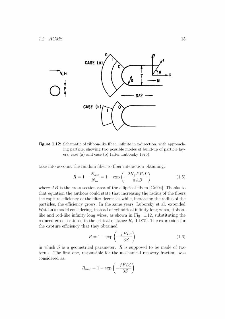
Figure 1.12: Schematic of ribbon-like fiber, infinite in z-direction, with approach-ing particle, showing two possible modes of build-up of particle lay-ers; case (a) and case (b) (after Luborsky 1975).
take into account the random fiber to fiber interaction obtaining:
R = 1 − Nout
Nin= 1 − exp
(
−2KfFRcL
πAB
)
(1.5)
where AB is the cross section area of the elliptical fibers [Gol04]. Thanks tothat equation the authors could state that increasing the radius of the fibersthe capture efficiency of the filter decreases while, increasing the radius of theparticles, the efficiency grows. In the same years, Luborsky et al. extendedWatson’s model considering, instead of cylindrical infinity long wires, ribbon-like and rod-like infinity long wires, as shown in Fig. 1.12, substituting thereduced cross section ε to the critical distance Rc [LD75]. The expression forthe capture efficiency that they obtained:
R = 1 − exp
(
−fFLε3S
)
(1.6)
in which S is a geometrical parameter. R is supposed to be made of twoterms. The first one, responsible for the mechanical recovery fraction, wasconsidered as:
Rmec = 1 − exp
(
−fFLζ3S
)

16 CHAPTER 1. FILTRATION AND HGMS
in which they introduced the reduced mechanical cross section parameter ζto take into account the traps due to the irregular disposition of the fibers.The other term, responsible for the magnetic capture, can so be expressedas:
Rmag = 1 − exp
[
−fFL(ε+ ζ)
3S
]
These results, and the analogue ones obtained by Uchima in the 1976 [Uch+76],suggested that not only magnetic particles, but also non magnetic ones, couldbe captured be randomly packed filter. To be aware of that effect Uchimasuggested to arrange the wires parallel to the main flow obtaining a simpleequation for the capture efficiency:
R = S∗cF (1.7)
in which the capture cross section S∗c is expressed as:
S∗c =
4
π
[
L
A
Vm
V0
]1/2
Uchima realized a prototype of filter with wires arranged that way achievinga good experimental agreement [HU80]. Aware of the limits comported bythe study of friction-less flow, in 1978, Birss and colleagues considered anidealized wires disposition in order to develop a model in which Newtonianfluid flow was considered [Bir+78b; Bir+78a]. In their model, thanks to arotational symmetry, they were able to model the system using a muffin-tinvelocity potential with fully radial symmetry obtaining as shown in Fig. 1.13:
R = 1 − vr0
v0
exp(−KFr2ia) (1.8)
in which v0 is the ideal velocity of the flow, vr0 is the velocity in rr0 (rr0
is the distance from the wire at which dv/dr = 0 and ria is a geometry-dependent distance. The improvements due to this new approach resultedlimited compared to a modified Uchima’s model [BPS80]. In recent yearsHerdem modified the model developed by Birss and Gerber introducing twonew parameters: the volume fraction of the wires in the system γ and themeasure of the non-circularity of the capture cross section af [HKA00]. Con-sidering N as the number of magnetic particles per unit volume entering thefilter they defined, for a unitary area, the number of particles entering perunit time as Nin = N 〈V 〉 where 〈V 〉 is the average velocity of the fluid inthe filter. In a similar way they defined Nout = Nne 〈Ve〉 where Nne is the

1.2. HGMS 17
number of non-captured particles per unit of volume and 〈Ve〉 the averageescape velocity. They expressed the probability that a particle would not becaptured as:
ω = (1 − afπa2r2
ca)n
where rca = rc/a is the capture radius; introducing the normalized capturecross section S∗
a they can rewrite it as:
ω = N(1 − afπa2S∗
a)n (1.9)
and assuming that S∗a ≈ 4
πL0.5
a the equation of the filter capture efficiencycan be written as:
R = 1 − exp
(
−4γaf
πL0.5
a
)
(1.10)
In 1988 Sandulyak experimentally improved that model writing a semi-empiricalrelation in the following form [San88]:
R = λ [1 − exp (−αL)] (1.11)
in which he introduced the ratio between the number of the magnetizableparticles and the total number of the particles λ and the empirical constant α,in general dependent on geometrical and magnetic properties of the system.A further, recent, improvement to the Sandulyak’s model has been developedby Abbasov et al. considering only the magnetic force Fm and the dragforce FD both in a simplified form [AKH99; AA02]. About the former they
Figure 1.13: (a) Array of wires with Wigner-Seitz cell. (b) Muffin-tin velocitywell around a wire (after Birss 1978).

18 CHAPTER 1. FILTRATION AND HGMS
described it acting on a particle near a wire as:
Fm ≈ πδ3
2
µ0χµ1.38H2
d(R/a)(1.12)
where χ is the effective susceptibility defined as χ = χp − χf (in which χp
is the susceptibility of the particle and χf is the one of the fluid), H is theexternal magnetic fluid and δ is the effective particle size. The drag forceacting on a spherical particle in a fluid of density ρf and with drag coefficientCD was stated to be:
FD ≈ CDπρfU2δ2/8 (1.13)
where U is the local velocity of the fluid. From these two equations, af-ter some maths necessary to express the relation between R/a and U , theydescribed the efficiency of the filter as:
R = λ
1 − exp[
−2.1 × 10⁻³(Vm/Vf)(L/d)αL]
(1.14)
The authors emphasized that eq. 1.14 was valid only for a very low Reynoldsnumber (Re << 1). In order to overcome this limitation they took in con-sideration also the lift component of the drag force obtaining the following:
R = λ
1 − exp
[
−2.12L
(
χH0.75δ
ρfV 2f d
2.7
)]
(1.15)
where the strong dependency of the filtering process on fluid velocity andparticle diameter are visible.
On another side there was some effort to develop a model for the filteringprocess based on the analysis of some dimensionless parameter. Herdem etal. defined the magnetic pressure parameter as [HKA00]:
PM =Kµ0µ
1.38H2(1 − ϕ)δL
d(1.16)
in which K is the effective magnetic susceptibility and d the filter diameter.Pm has the dimension of a pressure and depends only on magnetic values.They used eq. (1.16) in writing the logarithmic capture efficiency of the filteras:
β = 1.4 × 10⁻²
(
PM
∆P
)2(1 − ε
ε
)0.6
LD (1.17)
where LD is the length of the filter normalized with respect to d. A similarapproach was followed by Gerber in the case of randomly spaced sphericalmagnetic elements [GL89]:
R = λ
1 − exp
[
−5.36 × 10⁻²Ld
(
Pm
∆P
)0.6]
(1.18)

1.2. HGMS 19
A different side of the problem, often neglected in the literature because ofits over complications, is the one of the time evolution of the system. As saidit turns out to be very important, in particular in industrial applications, todetermine the breakthrough characteristics of the filters. Most of the studiesbased on the DBF resulted in a underestimation of the working time becausethe mass-balance model predicts the breakthrough characteristics startingdecreasing as soon as the filtration starts [CKT82]. The experimental analysis
Figure 1.14: The filtering efficiency Ψ as function of the time. The dashed curveis obtained from DBF model while the solid one is obtained from theexponential law described in eq. (1.19) (after Abbasov 2003).
shows that the filter efficiency remains almost constant in a first period, t0,drops down slowly in a second period, tW − t0, and stops working at a neartime, tS, as visible in Fig. 1.14. To describe that dynamic behaviour Koksalet al. proposed the following equation [KAH03]:
R = λ 1 − exp [α(t− tW ) − βx] (1.19)
where α and β are the capturing and detachment coefficients off the particles,respectively. The two parameters, considered as stochastic characters, must

20 CHAPTER 1. FILTRATION AND HGMS
be determined on the bases of the knowledge of the forces and phenomenons(such as pores and fibers saturation and detachment and recapture along thewhole filter) acting on the particles. They used the expression given in eq.(1.16) for β and defined α as:
α = 7.12 × 10⁻²ηvf
Dd
(
Pm
∆P
)−0.4
(1.20)
where D is the filtration velocity of the cleaner liquid. Considering tW ≈ 1/αthey derived:
tS =1 + βx
α
achieving a good agreement with the experimental behaviour of their filter.Another way is becoming followed nowadays: the computational ap-
proach. This latter method has been recently experienced in Japan by Okadaet al. [OM05]. They applied a Computational Fluid Dynamics (CFD) modelto simulate HGMS process with magnetic force, drag force and diffusion.The base equation of the problem is in the form:
∂
∂t(ρϕ) + ~∇ · (ρ~uϕ) = ~∇ · (Γ~∇ϕ) + S (1.21)
where ρ is the fluid density, ϕ is the transported scalar variable (in that casethe particle mass fraction), ~u the fluid velocity field, Γ the scalar diffusionconstant and S the scalar source term. From left to right, the four terms ineq. (1.21) are commonly referred as the transient, convection, diffusion andsource one. In order to solve the equation only the magnetic and drag forcesare considered. The particles are considered spherical and non-interactingand the fluid flow is a two-dimensional laminar one. The resulting systemis solved with a commercial, finite elements code able to describe the timeevolution of the system as the shape of the deposits changes. Anyway theproblem is still too oversimplified and the results are of quite small interest.
HGMS applications
The problem of separation is almost omnipresent in manufacturing and inindustrial production: from ore treatment to food, from steel purification topharmaceutics and so on [NS03]. Sedimentation and centrifugation are oftenused when speed is not an issue while magnetic separation can provide a fastermethod, especially if the removing substance has some magnetic properties[Hub+01; Fle91; Moe+04]. However, even in the absence of intrinsically mag-netic components the use of specifically designed magnetic beads, targeted

1.2. HGMS 21
(a) (b)
Figure 1.15: (a) Natural kaolinite. (b) Kaolinite after HGMS cleaning.
to the product of interest, can make a magnetic separation feasible for virtu-ally any system [Yav+09; Zha07]. Such processes offer very different kinds oftrade-offs in speed and selectivity as opposed to the more conventional ap-proaches. Limiting the review of the available applications of the magneticseparation to separation of material from liquids we can evidence one of themost important features when compared with solid state filters (membranes):in magnetic filter the pressure drop is virtually absent while for the mem-branes, particularly when talking of ultra-filtration (diameter of the particlesof the order of the micron) or nano-filtration (sub-micron diameters), theinduced flow resistance is very significant and a big amount of energy mustbe provided in order to maintain the flow through the filter. Moreover solidstate filters have to be changed or cleaned more often [KAH03]. A short listof the main actual applications of HGMS follows [Yav+06a; Yav+09]:
Kaolin de-colorization China clay (also known as kaolin) is a clay mixtureprimarily consisting of kaolinite mineral. The name cames from a Chi-nese region (Ching-te chen) where a particularly appreciated porcelainwas produced using that mixture. Today kaolin is primarily used inpaper manufacturing with two functions: as a filler between the pulpfibers and as surface coating for a white glossy finish. The color ofthe kaolin is influenced by the contained impurities, which are ofteniron-based as visible in Fig. 1.15a. Because of the resistance of thekaolin to chemical cleaning, HGMS has been used in kaolin industrysince the seventies leading to high quality kaolin as visible in Fig. 1.15band is nowadays responsible for more than 70% of the world productionof white porcelain and paper [Ode76]. A typical plant would have anHGMS with a filter diameter of 2m and a capacity up to 20t/h [HW82;

22 CHAPTER 1. FILTRATION AND HGMS
HBW82].
Paper Similar to the kaolin purification is the paper treatment to achieve amore white paper [NT06; Kak+04];
Steel factories On average, generating 1t of steel requires 151t of water forcooling and cleaning purposes; the resulting wastewater is filled withmany magnetic particulates and other iron-containing impurities andmust be cleaned [Ha+; Tas; Kar03]. The choice of HGMS as filteringtechnology has emerged a natural one saving a great amount of timeand space removing up to 80% of contaminants [Obe+75; HNW76].
Power plants and pollution In power plants (both conventional and nu-clear) HGMS is used to remove ferromagnetic or paramagnetic partic-ulates which extends the lifetime of cooling systems. Magnetic separa-tions can also be used to treat pollution. Fly ash from coal power plantsis 18% iron oxide. Magnetic filtration has been applied to capture 15%of waste fly ash, thus providing a means for recycling. Estimates showthat this can replace some of the magnetite used in industry [HBW82].
Ores separation The treatment of ores with magnetic separation is carriedout primarily on iron-containing ores. Conventional chemical and set-tling methods are not suited for this purpose given the similar densityand reactivity of transition metal minerals. The magnetic nature ofiron species, however, is unique and thus a natural target for magneticseparations. Among the iron ores taconite is most often subjected tomagnetic treatments. From a taconite ore (33% iron) Kellard was ableto recover iron at 95% on a 5 cm/s flow rate [Kel73]. Today, Metso Min-erals, Inc. (formerly Sala International AB) offers magnetic separatorsthat can separate iron from ores with nearly 100% efficiency (depend-ing on the particulate sizes, magnetic field and flow rate). Magneticseparation of pyrite (FeS2) from coal for desulfurization is also a com-mon process [MK78]. The weakly magnetic nature of pyrite, however,requires that the raw ore be pre-treated thermally to convert the pyrite(FeS2, Ms = 0.3emu/g) to more strongly magnetic pyrrhotite (Fe7S8,Ms = 22emu/g). Up to 91% removal of sulfur from coal can be achievedby microwave heating followed by a magnetic separation [UAA03].
Food industry Strict food quality standards require the food products tobe contaminant free, where mainly rare earth elements (REEs) consti-tute the majority. The food industry, therefore, has found magneticseparations to be an ideal method to remove REEs from food ingre-dients. Similar to the ore beneficiation or desulfurization, the target

1.2. HGMS 23
substances are weakly magnetic and require the high gradients of amagnetic field to be removed in a continuous food production line.Bunting Magnetics Co. offers magnetic metal separators and metal de-tectors for the quality of food and extended service life of the processingequipment, especially for cheese processing, chocolate plants, pet foodprocessing, flour mills, spice plants, vegetable processing. Removal ofboth ferrous and nonferrous tramp metals is achieved by their line offood safety products for the food processing industry.
Water treatment With new lowered maximum permissible concentrationfor arsenic in drinking water (10µg/l) in the USA in 2006 (ArsenicRule, 2006), techniques for better arsenic remediation without muchdesorption have gained more importance [SF03]. Currently, coprecip-itation, adsorption in fixed-bed filters, membrane filtration, anion ex-change, electrocoagulation, and reverse osmosis are methods of interest.However, cost efficiency and waste quantity requires further develop-ment that would aid in resolving the problem [Hos+05]. Arsenic ad-sorption and desorption are heavily influenced by adsorbent particlesize [May+07; Yea+05]. Nanoscale magnetite (Fe3O4, 12nm) can re-move 200 times better than its commercial counterparts, which allowsa significant cut in waste, instead of 1.4kg of bulk iron oxide to re-move arsenic (500µg/l) from 50l of solution, 15g of nano magnetite canbe used [Yav+06a; Yav+06b]. Apart from surface area increment, anobvious gain while going down to nanoscale, available open sites withthe proper chemistry (free Fe on the surface) can be accounted for thisunexpected result. Size dependent magnetic properties bring controlla-bility and along with mobility, a critical nanoscale advantage, providesunique applicability, if put in a system, in especially household useswhere electricity is not readily available [Mit+03]. In the seventies DeLatour and Kolm treated water samples from the Charles River (Fe3O4
seeding, 5 ppm Al3+) with a high flow velocity HGMS (V0 = 136mm/s,H0 = 1T ) and reduced coliform bacteria from 2.2×10⁵/l to 350/l, tur-bidity by 75%, color by 95%, and suspended solids by 78% [Lat73;LK75; GB83]. Later, Bitton and Mitchell removed 95% of the virusesfrom water by magnetic filtration following a 10min of contact periodwith magnetite (added to be 250ppm). The following years, BolidenKemi AB reduced phosphorus of water supplies at least 87% [GB83].Also known as Sirofloc process, micron-sized magnetite is also usedto remove color, turbidity, iron, and aluminum from water sources asan alternative to metal-ion coagulation [GMS88]. Recently, Denizli andcoworkers magnetically modified yeast cells for facile capture of mercury

24 CHAPTER 1. FILTRATION AND HGMS
with fast biosorption rates (within 60min) and efficiency (76.2mg/g forHg2+) [Yav+06a; Yav+06b].
Biotechnology The ability to control remotely inspired many biotechnol-ogists and medical scientists to investigate magnetic solutions for sev-eral biochemical processes, such as protein and cell separations andpurifications, magnetic drug targeting and delivery, and enzyme-basedbiocatalysis [Wu+04]. Unlike industrial applications, in-lab or batchapplications require tailor-made magnetic materials but remain finewith steady, not continuous, bench-top or batch, process solutions. Inorder to achieve bio-compatibility biochemists tend to use naturallyexisting minerals, such as magnetic iron oxides (magnetite, Fe3O4 andmaghemite, γ−Fe2O3), due to their biologically safe nature i.e. in theferrofluids [Tar+03; ACA05].

Chapter 2
Mathematical Model
The lack of knowledge related to the high gradient magnetic separationphenomenon limits its applicability and reliability, so that, as stated, it re-quires a more deep study on both the theoretical and the experimental pointsof view. The theoretical analysis of the process involve the study of a manybody system (a huge number of particles interacting with the ferromagneticmatrix has to be considered) on different scales (both particle scale and filterscale) at the same time. Moreover, at the microscopic scale, the consideredlaws of physics are often quite uncertain, being tested only at the macroscopicscale. The finite elements method, in a fully three dimensional approach, isnot affordable with an ordinary computer: considering the whole filter as aone cubic meter object and the elements of the ferromagnetic matrix havinglinear dimension on the micro-metric scale would lead to a mesh of, at least,1010 elements. As a consequence, approaches like the one of Okada [OM05]are limited to a bi-dimensional one. On the other side the study of the prob-lem starting from the single wire approximation with an analytical solutionis oversimplified and leads to not completely reliable results [WB86; Obe76].
The approach exposed in this chapter is used to develop a model whichis original and versatile, but applies to the experimental setup described inChapter 3 in particular. Its aim is to overcome both the exposed limitsthrough a mixture of a statistical approach and an analytical one. The prob-lem looks upon the removal of a hypothetical pollutant, for example arsenic,through its bounding into an iron oxide. The liked adsorption processes,which strongly depends upon the adsorbent dimensions, are well known andestablished ones [Oli+02]. Some typical reactions for heavy metals are shownin more details in Appendix B.1. As a consequence of this hypothesis theresulting problem concerns the removal of a given iron oxide from a workingfluid without caring about any specific pollutant. This possibility relies onthe assumption that the bounding does not change the magnetic properties
25

26 CHAPTER 2. MATHEMATICAL MODEL
of the iron oxide. This is a good assumption: being the bounding a super-ficial phenomenon while the magnetic properties are related to the volumeof the particles a relative influence is unlike. Starting from the study of an“average” element of the filter with analytically known induction field andvelocity field it turns out to be possible to study the particle trajectories.From the analysis of the trajectories in such a complex geometry is possibleto characterize the considered element. The element is then related to thewhole filter thanks to a model for the conservation of the number of theparticles.
2.1 The Cell
2.1.1 Cell geometry
As stated a magnetic filter is a macroscopic device with dimensions ofthe order of the tenth of a centimeter. The considered filter is an HGMS onein which the filtering element is constituted by iron steel wool with irregularshape and random disposition of the fibers (as visible in Fig. 2.1a). Sincethe spacing among the fibers of the wool are several orders of magnitudelower than the filter length and of unknown geometry, the magnetic field andthe fluid-dynamic regime has been determined in an elementary “mean” cell,using an integral model with spatially periodic conditions. The geometryof the fibres has been modelled with triangular prisms and tetrahedrons inorder to reproduce as much as possible the real geometry of the wool. Thecell is characterized by the packaging factor Γ which is defined as the ratiobetween the steel fibres volume and the cell volume:
Γ =Vwool
Vcell(2.1)
The distribution of the non-intersecting polyhedrons is chosen in order toobtain a given packaging factor Γ. The dimensions of the cell have to bechosen in order to keep the computational burden for the computers accept-able. On the other side the cell must be meaningful on the average. Thismeans that it’s not appropriate to consider a cell which contains only a fiber(nor an empty one). Considering fibers with transversal dimensions of theorder of 20µm a cell of 1mm × 1mm × 1mm has been chosen [Mar+09a].Moreover, the cell is enlarged with a frame of variable thickness in order toachieve a more correct boundary condition of the magnetic induction fieldand of the fluid velocity field. The thickness is chosen inversely proportionalto the packaging factor in order to contain a minimum, but non zero, number

2.1. THE CELL 27
(a) (b)
Figure 2.1: (a) SEM view of steel wool and (b) a possible random geometry of anelementary “mean” 3D cell
of fibers in it. An analysis has been carried out in order to check the validityof this approach: a large number of tests have been performed studying thechange in the trajectories when considering the cell surrounded by one ortwo layers of cell. The obtained trajectories turn out to be undistinguish-able (such as the magnetic field and for the velocity one), so that the cellapproximation resulted validated [Mar+09b]. The cell can be adapted to a2D flow considering long fibres made of parallel prisms, without bending andbreaking, in the central plane of the cell. Fig. 2.1a shows a SEM (ScanningElectron Microscope) view of a steel wool sample. Fig. 2.1b shows a ran-domly generated geometry for a cubic cell of 1 mm side. All the fibers areinteracting, i.e. they all contribute on equal basis, both to the velocity andflux density field within the cell. Anyway, the fibers are supposed rigid: nomechanical model of the drag and magnetic forces acting on them and corre-sponding displacements has been made. This means that the cell geometryis assumed to be unaffected by the external applied field.
2.1.2 Flux density field
As seen in Section 1.2.1 each particle is magnetized by a field which ismade of three terms: a relatively uniform field B0 produced by sources ex-

28 CHAPTER 2. MATHEMATICAL MODEL
ternal to the filter, a field produced by the ferromagnetic filter element (steelwool fibers) and the interaction field produced by the magnetic moments ofthe particles. Neglecting the latter and assuming that the stainless steel woolfibers are magnetized to saturation M, the flux density field can be directlyevaluated analytically from the known sources by superposition, i.e. addingthe fields produced by all the magnetized prisms and tetrahedrons of theperiodicized cell. Following Fabbri [Fab08; Suh00; Fab09] the magnetic fluxdensity B produced at the point r can be expressed analytically. By defi-nition, the magnetic vector potential produced by an uniformly magnetizedpolyhedron is given by:
A(r) =µ0
4π
∫
V
M× (r − r′)
|r− r′|3 d3r′ (2.2)
Being M uniform it can be rewritten as:
A(r) =µ0M
4π×∫
V
(r − r′)
|r − r′|3d3r′ =
µ0M
4π×∫
V
∇′ 1
|r − r′|d3r′ (2.3)
where a well known vector identity was used. Applying the Gauss’ theorem:
A(r) =µ0M
4π×∮
∂V
n
|r − r′|d2r′ =
µ0
4π
∑
Sf∈∂V
M× nf
∫
Sf
1
|r− r′|d2r′ (2.4)
where nf is the outgoing unit vector normal to the surface Sf . Defining theharmonic function Wf as
Wf (r) =
∫
Sf
d2r′
|r− r′| (2.5)
it can be proven that Wf and its gradient depend on the given polygonalface Sf , but they are independent of their orientation nf [Fab08; Fab08]. Itfollows that it is possible to write eq. (2.4) as:
A(r) =µ0
4π
∑
Sf∈∂V
M× nfWf (r) (2.6)
The calculation of B = ∇×A, assuming Wf differentiable, is straightforward.The total induction field in every point turns out to be:
Be (r) = B0 −∑
∀polyhedron
µ0
4π
∑
Sf∈∂V
(M × nf) ×∇Wf (r) (2.7)
The implementation of the former equation is achieved in a fast way, thanksto the analytical knowledge of the function Wf and its gradient. Fig. 2.2shows a detail of the map of the flux density field (arrows) and its squaredmodulus (color shading) inside a detail of a cell section.

2.1. THE CELL 29
0
0.2
0.4
0.6
0.8
1
1.2
1.4
1.6
1.8
B2[T
2]
-200 -150 -100 -50 0
[µm]
-400
-350
-300
-250
-200
[µm
]
Figure 2.2: Detail of the map of the flux density field (arrows) and its squaredmodulus (color shading) inside a cell section, obtained for B0 = 0.5T, µ0M = 1 T, Γ = 3.5 × 10⁻³ and with an average radial dimensionof the wool fibers of rc = 15µm.
2.1.3 Fluid Velocity and Pressure fields
A modification of the Method of Fundamental Solutions (MFS) [You+06]for incompressible steady-state 3D Stokes problems has been developed, thatapplies to 2D problems also. The Helmholtz decomposition theorem is usedto decompose the Stokes flow into the sum of a known potential flow anda viscous flow, so that the fundamental solutions are the solutions of thebi-harmonic equation for the stream function vector. As stated in [You+06;MSG99] the decomposition of the Stokes flow into the sum of a potential flowand a viscous flow leads to a purely boundary-type mesh-less method, par-ticularly suitable for exterior problems and for solving inverse or degenerateproblems in which missing or degenerate boundary data or the solutions at afew points within the domain are required. Moreover, comparing with otherformulations such as the velocity–vorticity and vorticity–potential there isa reduction of the number of variables that can decrease the computationaltime and the required storage. Once the unknown coefficients of the funda-mental solution are determined from the imposed no-slip velocity boundary

30 CHAPTER 2. MATHEMATICAL MODEL
conditions, the distributions of velocity and pressure over the entire compu-tational domain can be directly evaluated. Finally the method used is easyto implement, as far as the numerical algorithm is concerned, since it’s basedessentially on the same kernels of the magneto-static problem [Suh00].
The incompressible steady-state Stokes problem is governed by the con-servations of mass and momentum (neglecting the inertial term, that is withlow Reynolds number Re):
∇ · u = 0 (2.8)
−∇p + η∇2u = 0 (2.9)
subjected to the no-slip boundary conditions on the surface of the fibers inthe cell and to
u|∂cell = u0 (2.10)
on the cell boundary, where u is the velocity vector field, p is the pressure, ηis the dynamic viscosity, u0 is a known boundary velocity related to the massflow rate in the filter. The assumption of low Reynolds number is permissibleconsidering for the mean flow rate Q, the diameter of the particles dp, thearea Ahole of the holes crossed by the fluid the values in Table 2.1 and Table2.2 (that are the experimental conditions described in Chapter 3) obtaining:
Re =ρH2OQdp
πηH2OAhole≈ 10
Taking the curl of (2.9) with constant η, and using (2.8), we obtain thesteady-state vorticity transport equation for Stokes flows as follows:
∇2∇× u = 0 (2.11)
Equation (2.8) and the boundary condition (2.10) are identically satisfiedwith the Helmholtz decomposition:
u = u0 + ∇×Ψ (2.12)
provided that the solenoidal part zeroes at the cell boundary. Moreover, inorder to obtain uniqueness, the stream function vector Ψ can be constrainedto be solenoidal. Thus, from (2.11) and (2.12) we obtain the bi-harmonicequation for the stream function vector: ∇2∇2Ψ = 0. Finally, since theproblem is linear, the stream function vector can be expressed as the su-perposition of the contributions of the polyhedrons in the cells. In order todetermine the Green functions for a given polyhedron inside the cell, we start
2.1. THE CELL 31
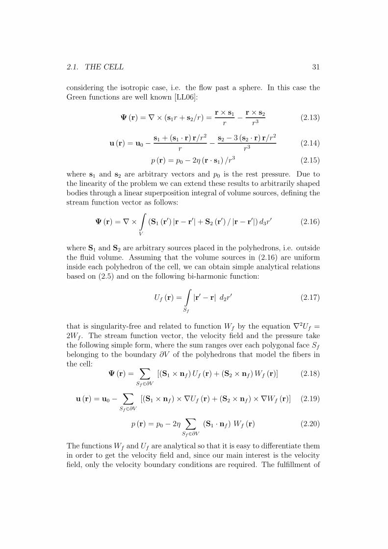
considering the isotropic case, i.e. the flow past a sphere. In this case theGreen functions are well known [LL06]:
Ψ (r) = ∇× (s1r + s2/r) =r × s1
r− r × s2
r3(2.13)
u (r) = u0 −s1 + (s1 · r) r/r2
r− s2 − 3 (s2 · r) r/r2
r3(2.14)
p (r) = p0 − 2η (r · s1) /r3 (2.15)
where s1 and s2 are arbitrary vectors and p0 is the rest pressure. Due tothe linearity of the problem we can extend these results to arbitrarily shapedbodies through a linear superposition integral of volume sources, defining thestream function vector as follows:
Ψ (r) = ∇×∫
V
(S1 (r′) |r − r′| + S2 (r′) / |r − r′|) d3r′ (2.16)
where S1 and S2 are arbitrary sources placed in the polyhedrons, i.e. outsidethe fluid volume. Assuming that the volume sources in (2.16) are uniforminside each polyhedron of the cell, we can obtain simple analytical relationsbased on (2.5) and on the following bi-harmonic function:
Uf (r) =
∫
Sf
|r′ − r| d2r′ (2.17)
that is singularity-free and related to function Wf by the equation ∇2Uf =2Wf . The stream function vector, the velocity field and the pressure takethe following simple form, where the sum ranges over each polygonal face Sf
belonging to the boundary ∂V of the polyhedrons that model the fibers inthe cell:
Ψ (r) =∑
Sf∈∂V
[(S1 × nf)Uf (r) + (S2 × nf )Wf (r)] (2.18)
u (r) = u0 −∑
Sf∈∂V
[(S1 × nf ) ×∇Uf (r) + (S2 × nf ) ×∇Wf (r)] (2.19)
p (r) = p0 − 2η∑
Sf∈∂V
(S1 · nf ) Wf (r) (2.20)
The functions Wf and Uf are analytical so that it is easy to differentiate themin order to get the velocity field and, since our main interest is the velocityfield, only the velocity boundary conditions are required. The fulfillment of

32 CHAPTER 2. MATHEMATICAL MODEL
-3
-2
-1
0
1
2
3
4
∆p[Pa]
-200 -150 -100 -50 0
[µm]
-400
-350
-300
-250
-200
[µm
]
Figure 2.3: Detail of the map of the velocity field (arrows) and of the pressure drop(color shading) inside a cell section for u0 = 14mm/s, η = 0.09Pa · s,Γ = 3.5×10⁻³ and with an average radial dimension of the wool fibersof rc = 15µm.
the boundary condition (2.10) and of the no-slip conditions would lead toan integral equation for the unknown sources that is avoided imposing thatthe velocity on the surfaces of the fibers is zero in the mean sense. Thus,for an arbitrary cell geometry, we impose the conditions of null velocityon a fixed number of points on the faces (outer fold) of the polyhedronsthat lead to an over-determined system for the components of the uniformvolume sources in each polyhedron, which is solved with a least squaresapproach. Note that the fluid dynamic and the magneto-static problemsshare the same cell geometry. Both are based on the fundamental solutionsof their governing equations, and their solution methodologies do not dependon the discretization of interior computational regions [Suh00]. Unlike themagneto-static problem where the sources are known, the basic concept ofthe fluid-dynamic problem is to find the solution of the partial differentialequations (2.8) and (2.9) by superposition of their fundamental solutionswith sources of proper intensity. Since the method locates the sources outsidethe computational domain, no special treatments for the singularities of theGreen functions are required. However the way we impose the boundary

2.1. THE CELL 33
conditions “on average” leads to an error near the edges of the fibers thatis visible in Fig. 2.3, where, near the top corner of the top left section oftetrahedron, the velocity doesn’t approach zero the right way. Anyway we canneglect this effect acting on the stopping criterion in the particle trajectorycalculation. This approach is essentially 3D, but can be easily adapted to a2D problem also, as shown in Fig. 2.3.
2.1.4 Particles trajectories and capture parameter
Each particle is supposed spherical, suspended in the fluid flowing throughthe wool and only subject to the magnetic force and to the fluid drag force,expressed by the Stokes’ relation [LL06]. Since wastewater with a low concen-tration of the particles and at room temperature is considered, the gravita-tional force, the randomizing effects of Brownian motion and the interactionfield among particles have been neglected [MHB05]. The non-interaction ofthe particles is justified by the assumption of a low particle concentration.About gravity force and Brownian motion we can consider particles of diam-eter d = 10−6m, a mean velocity field u0 = 0.1m/s, the dynamic viscosityη = 10−3Pa/m, an induction field Be = 0.5T and gradient ∇Be = 104T/m,an effective magnetic susceptibility χ = 1, a working fluid temperature of300K and the density of the particles ρ = 5×10³kg/m3. Defining the Boltz-mann energy associated to the Brownian motion as:
EB = kBT
and using, for the drag force, the Stokes’ approximation:
Fd = 3πηdu (2.21)
we can calculate the following ratios to demonstrate the stated negligibility:
EB
EK=
kBT
1/2ρV u2≈ 10−4
Fg
Fd=
ρd2g
18ηu≈ 10−11
Fg
Fm
=ρgµ0
χBe∇Be
≈ 10−5
where EK is the kinetic energy of a particle, V its volume, Fg the gravity forceacting on a particle and Fm the magnetic one. Thus, the trajectory of oneparticle is independent from all the others and can be obtained numericallyintegrating its dynamic motion equation:
Vpρpd2x
dt2= 3πηdp
(
u (x) − dx
dt
)
+Vpχp
2µ0
∇B2e (x) (2.22)

34 CHAPTER 2. MATHEMATICAL MODEL
where x is the time-dependent position of the particle, ρp is the density ofthe particle matter and dp the particle diameter. Note that the last term of(2.22), obtained from (1.1), shows that the magnetic force is proportional tothe gradient of the squared modulus of the flux density. It follows from thevectorial identity:
∇(|B|2/2) − B · (∇B) = B × (∇×B)
thanks to ∇× B = µ0J = 0. Using a dimensional analysis we can write eq.(2.22) in term of x∗ = x
rcand t∗ = |u0|t
rc(in which rc is the average radial
dimension of the wool fibers):
x = rcx∗
t =rc
|u0|t∗
⇒
dx
dt= |u0| ·
dx∗
dt∗
∇ =1
rc∇∗
obtaining:
ρpd2pu0
18ηrc
d2x∗
dt∗2+dx∗
dt∗=
u
u0
+
d2pχpB0M
36rcu0η
∣
∣
∣
∣
∣
∣
µ0M
B0
∇∗
(
∑
polihedrons
φ
)2
+ 2∇∗B ·∑
polihedrons
φ
∣
∣
∣
∣
∣
∣
(2.23)
in whichφ =
∑
Sf∈∂V
(
M × nf
)
×∇Wf (x)
and the ˆ symbol stays for unitary vector. From eq. (2.23) we define thefollowing parameter:
Ω =d2
pχpMB0
36ηu0rc
(2.24)
which takes into account the relative influence of the drag and the magneticforce acting on a particle. A second parameter, Ωm = µ0M
B0, is ignored since it
is constant for given outer field and wool matter. Moreover, consistently withthe hypothesis of a low Reynolds number used in the calculation of the fluidvelocity field u, the comparison of the inertial force magnitude Vpρpu
20/rc to
the drag and the magnetic force shows that the left hand side of (2.22) isnegligible in the following limits:
Vpρpu20
rc
≪ 3πηdpu0 ⇒ u0 ≪18ηrc
ρpd2p
(2.25)
Vpρpu20
rc≪ VpχpMB0
2rc⇒ u0 ≪
√
χpB0M
2ρp(2.26)

2.1. THE CELL 35
Figure 2.4: Some trajectories obtained from the integration of eq. (2.27) in a twodimensional cell. On the floor of the cell its real dimensions are visible.
Thus the trajectories, obtained integrating the quasi-static equation
dx
dt= u(x) +
d2pχp
36ηµ0
∇Be2(x), (2.27)
depend only on the capture parameter Ω, on the starting point and on the cellgeometry, i.e. on the packaging factor [YYT00]. Equation (2.22) and (2.27)have been integrated numerically in a cell with the 5th order Runge-KuttaMethod [AP98]; it is assumed that the Van Der Waals force are localized onthe fibers boundary so that, when a particle is near a wire (i.e. its distancefrom the wire is less than its diameter), we can consider the particle stopped[Kir00]. An example of trajectories integration is shown in Fig. 2.4. Definingthe capture (or retention) efficiency σcell of a cell as the ratio between thenumbers of captured and entering particles [Tso+06], we characterized itfrom a statistical point of view. The capture efficiency, for a fixed Ω, is ob-tained generating 5-10 different random cell geometry (for every packagingfactor Γ) and studying 20-50 randomly starting trajectories of the particles.The numbers of the geometries and of the trajectories were chosen in orderto reach a low statistical error but containing the computational time too.Every trajectory could give two opposite results: captured or passed through(usually through the face of the cell opposite to the entering one). Figure 2.5shows the obtained capture efficiency: as visible it increases with Ω, i.e. it

36 CHAPTER 2. MATHEMATICAL MODEL
0.005
0.01
0.05
10-610
-510-410
-310-210
-110010
1102
0.0
0.2
0.4
0.6
0.8
1.0
σ
Γ
Ω
σ
Figure 2.5: Capture efficiency σ of a cell as a function of the capture parameter Ωand of the packaging factor Γ from the integration of the quasi-staticequation.
increases with B and M and decreases when u0 or rc grow. It is also possibleto see that σ increases with Γ, that is as the distance between the fibersdecreases. In Fig. 2.6 the points represent the obtained average value of thecapture efficiency of a cell (σcell) for the two considered models (dynamic, eq.(2.22), and quasi-static, eq. (2.27)) when a specific packaging factor is con-sidered to improve reliability and readability. The bars are obtained as thevariance of the same set of geometry-trajectories results. The integration ofthe quasi-static equation (2.27) is at least two times faster than the integra-tion of the dynamic one (2.22). In Fig. 2.6 the marker symbol correspondsto the stronger lower limit on Ω for the validity of the quasi-static model,as obtained from (2.25) and (2.26). It has been calculated using the valuesshown in Table 2.1 which refers to the experimental set-up described in Chap.4. As shown in Fig. 2.6 the results predicted by the two models are quitesimilar for all the range of Ω investigated, also below the theoretical limitingvalue. It’s worth to note that both the quasi-static and the dynamic modelswould give a non-zero capture efficiency also without magnetic field applied.In fact, the stream lines tend asymptotically to zero, but the particles, havinga finite radius, may touch the fibers for every unperturbed velocity, providedthe right starting point is choosen: indeed, if the maximum fiber to fiber dis-tance would be less than the particles minimum radius every particle would

2.1. THE CELL 37
0.1 0.2
0.5
1
-10 -8 -6 -4 -2 0 2 4
σ cel
l
Log Ω
Ω=d2pχpMB0/36ηu0rc
σcell=(captured/entering)particles
Γ=3.5×10⁻³±30%
*
Quasi-staticDynamic
Figure 2.6: Capture efficiency σ of a cell as a function of the capture parameter Ωfor a given wool packaging factor Γ from the integration of the dynamicequation (green) and the quasi-static one (red). The bars show thevariance. The marker corresponds to the lower limiting value of Ω forthe validity of the quasi-statyc results.
Table 2.1: Reference values for powder (hematite), wool (AISI 434) and workingfluid (water).
dp χp [Oka+02] µ0M [BCD03] B0 [Fab+08] rc [Gmt] η0.8 ± 20%[µm] 2 × 10⁻³ 1[T ] 0.5[T ] 15[µm] 1 [mPa·s]
be captured, like in a sieve.
We can simply deduce the capture efficiency of the whole filter σfilter fromσcell, in the well verified hypothesis that the particles exit the cell throughthe face opposite to the entering one. In fact, by definition, knowing theaverage number of cells Ncell the flow pass through and supposing Ω and Γbeing constant in all the cells, the filter capture efficiency can be determineddirectly as follows:
1 − σfilter = (1 − σcell)Ncell (2.28)

38 CHAPTER 2. MATHEMATICAL MODEL
Tank
&
Stirrer
0 s1
s3 0
Filter Measurement
sections
0
s2
Upstream Line
Downstream Line
FR1
FR2
Figure 2.7: Scheme of the experimental set-up.
2.2 System mass balance
The passage from the cell model to the whole filter one is developed inthis section. Stating from elementary considerations about the conservationof mass it’s possible to describe the number of particles in a (closed) circuitin which some kind of deposition occurs. The expression, which, providedthe initial condition, results a function of time, is comparable with the exper-imental measurements of the concentration, as will be shown in Chapter 3.In the considered experimental set-up, whose scheme is shown in Fig.2.7, thefluid flows inside a closed-cycle circulating system thanks to a pump. Theflow starts from a 1l tank, visible in Fig. 2.8, filled with a mixture of waterand particles with an initially known concentration and returns to the samereservoir after passing through two lines and, optionally, the magnetic sepa-ration unit in the middle of them. The concentration ci,k in the experimentalset-up has been modelled through a set of local mass balance equations likethe following:
V0∂∂tbk(t) = −Q [C3,k(L3, t) − bk(t)]
bk(0) = bk(2.29)

2.2. SYSTEM MASS BALANCE 39
Figure 2.8: Picture of the tank used in the circuit.
Table 2.2: Geometrical parameters of the experimental circuit.
A0 · · · V0
[
m3]
1.00 × 10⁻³
A1
[
m2]
0.30 × 10⁻³ V1
[
m3]
1.00 × 10⁻³
A2
[
m2]
0.80 × 10⁻³ V2
[
m3]
0.25 × 10⁻³
A3
[
m2]
0.30 × 10⁻³ V3
[
m3]
0.50 × 10⁻³
for the tank and:
Ai∂∂tci,k(si, t) = −Q ∂
∂sici,k(si, t) − λi,kAici,k(si, t)
ci,k(si, 0) = ci,k(si)ci,k(0, t) = bk(t) , i = 1ci,k(0, t) = ci−1,k(Li, t) , i = 2, 3
(2.30)
for the lines and the filter. Q is the volume flow-rate, the index i refers tothe sections in which the circuit is divided (tank 0, upstream line 1, filter2, downstream line 3): Ai represents the area of each section, Vi its volume,si the distance in the relative one-dimensional reference system of each pipewhose length is given by Li = Vi/Ai. The mass balance equation for theconcentration bk in the tank (A0) lacks of the spatial gradient that has beenomitted due to the presence of a stirrer which provides homogeneity. Thestirrer, visible in Fig. 2.9, was realized in LIMSA laboratory to fit the spe-cific situation requirements. Table 2.2 shows the geometrical parameters ofthe experimental system. Since both eq. (2.22) and eq. (2.27) dependson the particles diameter, each powder is divided into populations sharingsimilar properties, according to the experimental size distribution (see Ap-

40 CHAPTER 2. MATHEMATICAL MODEL
Figure 2.9: Picture of the stirrer realized at LIMSA.
pendix C.1). The index k stands for the powders populations, being ci,k thepowder concentration in the section i for the population k. The experimentalconcentration xi is the sum of the single concentration:
xi(t) =∑
k=I,II,III
ci,k(si, t) (2.31)
Every population is decaying with a rate λi,k which takes into account bothspatial (essentially in the filter) and temporal (essentially in lines, due tosedimentation and walls adsorption) decay rate of the particles. In the filterthe decay rate for each population is related to the filter capture efficiencyfor the same population, by definition, by
1 − σfilter,k = e−λ2,kV2/Q (2.32)
which, considering that, as described later and visible in Appendix C.1, onlypopulation 2 is important in order to verify the model the relation can besimply written as:
1 − σfilter = e−λ2,IIV2/Q (2.33)

2.2. SYSTEM MASS BALANCE 41
The analytical integration of eq. (2.29)-(2.30) leads to a set of equations likethe following:
xi(t) =∑
k
e−λk
“
Vk−1Q
−AkQ
sk
”
bk
(
t− Vk−1
Q− Ak
Qsk
)
·
· U(
t− Vk−1
Q− Ak
Qsk
)
where U(t) is the Heaviside step function. This equation shows that, foreach population, the resulting concentration is the product of two differentbehaviours: there is a front periodical wave resulting from the concentrationin the tank and a decay due to the deposition. It’s worth to note that themodel has been developed in the hypothesis of high velocity, i.e. neglectingthe parabolic velocity profile in the pipe present in laminar flow. In differ-ent words I commited an error considering only a mean velocity for eachcross section of the pipe. Anyway the committed error is negligible: bothof the discussed characters of the concentration (periodic wave and decay)will be visible in the experimental measurements. The equations have beennumerically integrated imposing, for each population, the continuity of theconcentration through the contiguous sections. The main unknowns are theflow rate of the circuit, Q, the decaying constants, λi,k, and the mass fractionsfor each population in the initial sample, mk, which have to be determinedfitting the experimental results. To check the experimental condition twophases are considered:
A calibration one in which the filter is not inserted, the two lines are filledwith clean water and the tank is filled with a known particle concen-tration. Unlike what one would expect the decaying rate is nonzerobecause the population with the lower mean diameter is adsorbed bythe walls of the circuit. In this phase the oscillating part of the solutionis evident and so it is useful for the calculation of the flow rate and forthe calibration of the concentration meters (described in section 3.3).
A filtering one in which, after phase one, the filter, filled with clean water,is inserted between line 1 and line 3. Here the decaying rate of the filteris measured, from which the capture efficiency will follow as shown ineq. (2.33).
The fitting will be performed over each measuring experience and the ob-tained parameter averaged.

42 CHAPTER 2. MATHEMATICAL MODEL

Chapter 3
Experimental Set-Up
In order to verify our model I designed and built a laboratory device.The first prototype, visible in Fig. 3.1, was constituted by an open circuit.Starting from a tank the working fluid was moved to a second one passing
Figure 3.1: Photo of the first experimental set-up.
43

44 CHAPTER 3. EXPERIMENTAL SET-UP
through the filter. The first of the two tanks, each of 100l of capacity, wereinitially filled with at least 20l of water in order to achieve a working timeof around 5min. During each experience the desired quantity of powder waskept in suspension through human mixing. Anyway the working time re-sulted short and the results of difficult interpretation. In fact the continuousfiltration of a constant quantity of powder resulted in the saturation of thefilter (or at least of some of the cells interested in the separation process)requiring a different model of the phenomenon. To overcome these problemsthe model visible in Fig. 3.2 has been designed and realized. The schemeof the prototype is visible in Fig. 2.7. As visible, the hydraulic circuit isa closed one: starting from the tank, which is provided with a stirrer, theworking fluid is moved through the filter by the electric pump BE-M 20,NOVAX 20 capable to erogate a maximum power of 340W , made in Italyby ROVER, posed after the tank. A stirrer working inside the tank is notmandatory, but necessary in order to achieve a uniform initial concentrationof the working fluid in the tank and to avoid gravitational deposition of theparticles. The measuring instruments are collocated, after the tank, in thefollowing order:
• a barometer;
• a valve (to control the volume flow rate);
• a second barometer;
• a concentration meter (FR1);
• a second concentration meter (FR2);
• a volume flow integrator.
The filter is placed between the first and the second concentration meters. Allof them are connected via a transparent gum pipe of inner diameter 18mm.Every instrument, including the filter, was easy to remove from the circuitletting it in a working condition.

45
Figure 3.2: Photo of the experimental set-up.

46 CHAPTER 3. EXPERIMENTAL SET-UP
3.1 The filter
Figure 3.3: Hysteresis cycle of AISI434steel [BCD03].
The filter was made of stainlesssteel AISI434 wool with fibers of ef-fective diameter lower than 30 µm,obtained from GMT Inc. [Gmt] inthe form of rolls of diameter of about30cm, as visible in Fig. 3.4. Thefibers of the wool, as visible in Fig.2.1a, are similar to long prisms withtriangular cross section [Mas+06].The wool magnetization, as visiblein Fig. 3.3 is of about 8 × 10⁵A/mat saturation. The packaging of thewool required some attentions. Infact the first attempts, in which the wool was simply inserted in the tube,led to the formation of channels through which the flow is facilitated, as visi-ble in Fig. 3.5. After some attempts I developed a more performing filtering
Figure 3.4: Picture of a roll of iron steel wool.

3.1. THE FILTER 47
Figure 3.5: Picture of a filter packaged in the wrong way: a channel through withthe flow is facilitated is visible.
element, where the wool envelops a drilled test-tube to force the water toflow radially through the wool as shown in Fig. 3.6a-3.6b [Fab+08]. Theholes in the test-tube, each with a diameter of about 1.5mm, are disposedinto nine rows of three. As shown in Fig. 3.6c it is placed in a transparenttube, with a rectangular inner cross section of 24×40mm2 and an outer oneof 34 × 60mm2. The tube itself is placed in the air gap of the magnet, asvisible in Fig. 3.6c. It is possible to place a light behind the tube to improvethe filtering element visibility. The transparent tube can be filled with oneor two filtering elements. The hand made filtering elements are disposed asordinary litter after one usage.The flux density field source consists of a pair of PM made of six Sm-Co
XGS26 ingots 70mm × 70mm × 30mm provided by SAIMAG s.r.l., havingnominal remanence of 1.05T oriented perpendicularly to the wide face, sepa-rated by a gap of 40mm and coupled with a movable magnetic circuit madeof laminated M330-50A steel (Fig. 3.7a). The measured map of the trans-verse component of the flux density field produced on the central plane of

48 CHAPTER 3. EXPERIMENTAL SET-UP
(a) (b)
(c)
(d)
Figure 3.6: Images of the filtering element: opened (a) closed (b) and in the mag-net airgap (c) before an experiment and (d) opened after an experi-ment.

3.1. THE FILTER 49
(a)
0 5
10 15
20 25 0
1 2
3 4
5 6
0.0
0.1
0.2
0.3
0.4
0.5
B[T]
x[cm]
y[cm]
B[T]
(b)
Figure 3.7: Image of the PM (a) and map of the transversal magnetic flux densityfield (b).
the experimental system is shown in Fig. 3.7b. The measure was performedwith the LAKESHORE Gauss probe HMNT-4E04-VR. A maximum value of500mT is detected. This value is decreased by 20% in the inlet and outletregions of the filter. The other components are negligible in the filter region.The stray field at 50cm from the magnets is well below 5mT .

50 CHAPTER 3. EXPERIMENTAL SET-UP
3.2 The powders
In order to simulate the adsorbent we initially bought some magnetite’powder from Kremer Pigmente GmbH and, following the producers’ con-ventional name, labeled it #48800. The powder1 is normally used in themanufacturing of painting and is very cheap (between 5e and 10e per kg).The size distribution of that powder, shown in Fig. 3.8a, was measured us-ing FRITSCH Laser-Particle-Sizer “Analysette 22”. The measure was madein the laboratory of the Chemical, Mining and Environmental EngineeringDepartment of the University of Bologna (DICMA). The first observationof the working fluid, made in test tubes filled with water, shows that themagnetite dynamic viscosity in water resulted in a very fast deposition ofthe particles. In fact the time constant for sedimentation was of the orderof seconds. To avoid particle deposition we decided to use cooking-oil asworking fluid, which resulted in a very low deposition velocity. The effec-tive magnetic susceptibility of that ferrimagnetic powder, measured with adynamo-meter in the LIMSA laboratory, is about 1.4. However the particlesturn out to strongly aggregate when magnetized and to be very sensitive tothe external magnetic field gradient. In order to test our model we decidedto reduce the magnetic susceptibility of the working powder and we boughttwo different size-distribution samples of the same specie of hematite. Theirmagnetic susceptibility is known to be ≈ 2 × 10⁻³ [Oka+02]. The two dif-ferent hematite powders were obtained from Kremer Pigmente GmbH andlabeled #48100 and #48651. Figure 3.8b shows the frequency of the par-ticle size distribution of both powders measured using the same FRITSCHLaser-Particle-Sizer “Analysette 22” used for #48800 at DICMA. Neglect-ing the peaks on the left due to the instrument limits, it can be seen thatthe distribution is approximatively log-normal for all the three powders (asshown in Appendix C.1). Three populations with uniform properties havebeen considered for each powder: a central one labelled I and other two,labelled II and III, that take into account the lower and higher diameters,respectively. The deposition rate of powder of hematite resulted lower thanthe one of the magnetite letting us decide to use water as working fluid witha time constant for sedimentation of the order of the minutes.

3.3. THE MEASURING SET-UP 51
0
1
2
3
4
5
6
7
8
1 10 100
Freq
uenc
y %
Diameter [µm]
#48800
(a)
0 2 4 6 8
10 12 14 16 18 20
0.1 1 10
Freq
uenc
y %
Diameter [µm]
#48100#48651
(b)
Figure 3.8: Experimental size distributions for the magnetite powder (a) and forthe two hematite ones (b).
3.3 The measuring set-up
3.3.1 Concentration
The particle concentration inside the working fluid was measured bymeans of two homemade concentration-meters. They are homemade becausecommercially available ones are too limited. In fact they usually work with
1As well as the ones discussed later

52 CHAPTER 3. EXPERIMENTAL SET-UP
only a particular working fluid (such as water or oil only, with no possibil-ity of change). Moreover they usually work on samples while, to operatecontinuously, a on-line instrument was necessary. Each concentration-meteris made with a couple of Silonex NORPS-12 light-dependent resistor (Fig.3.9 and Fig. C.9 in Appendix C.4) and Kingbright L-7678C2VGC-H “su-perflux” led lamp (Fig. 3.9 and Fig. C.8 in Appendix C.4)) placed one infront of the other and with the gum pipe between them as visible in Fig.
3.10. The light dependent resistor, whose circuital symbol is wherethe arrows stand also for the positive terminal, is characterized by a max-imum response as function of the frequency of the incident light around6KHz, has shown in Fig. C.10a (in Appendix C.4). The chosen led emitslight, following the distribution shown in Fig. C.10b (in Appendix C.4), asa maximum emission around 6KHz too so it is compatible with the lightdependent resistor. We suppose the concentration of the powder related toturbidity of the working fluid by a linear function. The turbidity itself de-termines the ratio of the light which, emitted from the led lamp, is adsorbedby the powder, i.e. the ratio of the light which hit the photo-resistor. Theintensity of the light and the measured resistance are related by a log− log,relation as stated by the manufacture [Nor], so that the resulting relationbetween concentration and measured resistance is, in the working range ofthe photo-resistor, in the form (see Appendix C.2): C = a + b ∗ logR.
Figure 3.11: Image of the mea-suring circuit.
A third turbidity-meter FR0, described inAppendix C.3 has been made in order tomeasure the concentration of samples col-lected into test tubes. In order to ac-quire the resistance on the photo-resistor we
Figure 3.9: Picture of the led (left) and of the light dependent resistor (right) usedin making the concentration meters.

3.3. THE MEASURING SET-UP 53
Figure 3.10: Picture of a concentration-meter. The led lamp (powered) is on theleft side of the pipe while the photo-resistor is on the right side. Inthe upper right corner a hat used to avoid the environmental lightmodifying the measured value is visible. On the left it is visible R0.
used a Personal Computer equipped withGNU/Linux Real Time Application Inter-face [BMN06] coupled to National Instru-ment PCI-MIO-16E-1 I/O terminal with asampling rate of 10Hz. The schematic cor-responding to the two circuits shown inFig. 3.12 are realized with SCILAB/SCICOS[BB05]. Figure 3.12a shows the schematic rel-ative to the led supply while Fig. 3.12b showsthe one relative to the resistance acquisition.Figure 3.13 shows the graphical user inter-face (GUI) used to control the acquisitionprocess. That GUI was provided with theRTAI source code and compiled for the spe-cific hardware during the initial set-up of the software-side acquisition system.In Fig. 3.13 the mainly used components of the GUI are shown:

54 CHAPTER 3. EXPERIMENTAL SET-UP
(a)
(b)
Figure 3.12: Schematic of the acquisition system, made with SCILAB/SCICOS.(a) Led survey and (b) resistivity acquisition.
scopes that, like real ones, are able to show the measured quantity for everyused channel (with different colours) and save them on files;
meters that show the desired quantity in a dynamic way, for example, onthe right low corner, a clock measuring the (real-)time of the runningprocess is shown;
panels used to set varius parameters.

3.3. THE MEASURING SET-UP 55
Figure 3.13: Screen-shot of the xrtailab graphical user interface used to controlthe acquisition process.
Given a fix voltage Vtot = 5V over a serie constituted by a known resis-tance R0 and the one of the photo-resistor RFR as visible in Fig. 3.11, theacquisition system gave the last one as:
RFR = R0
(
Vtot
V0
− 1
)
(3.1)
where V0 is the voltage over R0. It is possible to determine the concentrationof the powder in the working fluid for a given working condition with twoknown values of the C-RFR couple. The first couple of points is providedby a calibration phase (as described in Section 2.2). That phase, which isperformed during every experiment, consists of a 600sec measurement witha known initial concentration and without a filtering element. Moreoverthe initial concentration, even if the powder is weighted with an accurateGALILEO-SARTORIUS balance (with an absolute error of 10−2g), is sub-jected to inaccuracy, mainly because of the uncertainty about the workingfluid volume. The calibration phases are, for example, visible as the leftcurves in Fig. 4.2-4.3. The right curves in the same figures are obtained af-ter turning off the pump, inserting the filter and turning on the pump again.

56 CHAPTER 3. EXPERIMENTAL SET-UP
0.04
0.06
0.08
0.1
0.12
0.14
0.16
0.18
0.2
0.22
0.24
0.26
50 100 150 200 250 300
Q [
l/se
c]
faucet opening [°]
Figure 3.14: Image of the measured correlation between the valve opening andthe volume flow rate.
The second couple of C − R points is choosen at the end of the filtrationphase. In fact, a 0 − 0 couple is usually usually reached. Moreover, for thefitting, a more precise value for that couple is obtained measuring the con-centretation of a corrisponding sample with the off-line concentration-meter(see Appendix C.3).
3.3.2 Volume flow rate and temperature
The measure of the volume flow rate was initially performed with three,independent, methods:
• direct measure with the volume flow rate integrator;
• pressure drop estimation;
• mass-balance-model-parameters fitting.
The results were compared to choose the best approach, which turned out tobe the last one. In fact the error of the volume flow rate integrator resultedvery high for slow flows. The two barometers 111.12, made by WIKA, aredesigned to work between 0bar and 2.5bar with an error of 0.1bar [Bar].They are inserted with the valve between them, to give us the knowledge ofthe volume flow rate which is proportional to the pressure drop [LL06], but

3.3. THE MEASURING SET-UP 57
with a big error too, due to a sort of hysteresis in the opening-closing loop.The measure of the pressure drop due to the wool constituting the filteringelement resulted unaffordable because of the low packaging factor.
Anyway a correlation between the valve opening and the volume flowrate was deduced and gave us the possibility of choosing the desired rangeof volume flow rate as visible in Fig. 3.14. More reliable values were thenobtained from the fitting of the parameters involved in the particle balancemodel (Section 2.2). The resulted value turned out to be dependable in allworking conditions.We regularly checked the temperature of the working fluid with a thermo-couple connected to a MITEK MK1330 multi-meter. The temperature turnedout to change, probably because of the pump heating, from a room temper-ature of about 25C to about 35C whithout any appreciable influence onthe separation process.

58 CHAPTER 3. EXPERIMENTAL SET-UP

Chapter 4
Measurements and results
As stated in Chapter 2 and in Chapter 3 the used RTAI acquisition sys-tem is able to collect measured values of voltage and, from them, calculatethe corresponding resistances. The resistance is then transformed into themore interesting concentration. This is done through the C = a + b logRrelation between concentration and resistance (see Appendix C.2, eq. C.3).That relation needs to be fitted for every experimental condition in order todetermine the two parameters a and b. In fact during each experience thepipes between the leds and the light-dependent resistors get dirty and, even ifthe following cleaning is accurate, the subsequent starting conditions are sig-nificantly different. Moreover, while cleaning is performed, some twisting ortorsion is occasionally transmitted to the two active elements changing theiralignment and, consequently, to the range of the intensity of the incidentlight [Mar+10].
4.1 Measurements
4.1.1 Rough results
Magnetite #48800
The first experimental campaign has been carried out using the #48800magnetite to simulate the adsorbent. The high deposition velocity led to theuse of cooking oil as working fluid, thanks to its higher viscosity compared towater (Fig. 4.1a). Anyway the high magnetic susceptibility of the magnetitepowder caused two undesired phenomenons:
1. auto-aggregation of the particles so that the un-interacting particleshypothesis resulted wrong;
59

60 CHAPTER 4. MEASUREMENTS AND RESULTS
2. as a consequence of 1 the gradient of the magnetic field due to the com-posite nature of its source (three ingots for each face) resulted enoughto retain particles, as visible in Fig. 4.1b.
This problem, well visible in Fig. 4.1, implies the inapplicability of ourmodel so that the experiments carried out with the magnetite powder resulteduseless with respect to what exposed in Chapter 2 and in Chapter 3. Anywaythe model, being a general purpose one, is able to predict the behaviour ofthe magnetite powder at lower granulometry, i.e. with an higher adsorbent
(a) Picture of the filtering process with filtering element
(b) Picture of the filtering process without filtering element
Figure 4.1: The pictures show a filtration moment, with and without filtering el-ement, for the magnetite powder #48800. The comparison illustratesthe inapplicability of the developed model to the considered experi-mental conditions.

4.1. MEASUREMENTS 61
specific surface. In that situation the capture would be good enough for mostapplications with a very high adsorbing efficiency.
Hematite #48100 and #48651
To test the developed model in a congruent way the two hematite #48100and #48651 had been chosen. Their magnetic susceptibility is in the range ofparamagnetism so that no undesired phenomenon, such as capture in slowlyvarying magnetic fields or particle-particle interaction, arise. Moreover thehematite density and viscosity (relatively to water) resulted such that depo-sition velocity was quite low and water usable and consequently chosen asworking fluid. After some initial test the working parameters for the circuitdescribed in Table 2.1 were chosen as:
C0 , the initial concentration, was chosen equal to 0.2g/l in order to avoiddeposition and clogging on the filtering element. The resulting masswas mp = Vtot ∗C0 = 0.55g, where Vtot = V0 + V1 + V2 + V3 = 2.75l (seeSection 2.2).
u0 , the unperturbed velocity in the filtering element region, is determinedfrom the flow rate, on the basis of the effective area of the drilled holesin the pipe. Considering a flow rate Q of about 0.15l/s, i.e. the valveopening equal to about 180, the resulting velocity is u0 = Q/Atot ≈0.2m/s, where Atot = 27π(dh/2)2 ≈ 50mm2. It’s worth noting thatwith this opening the pressure drop on the filter, as stated, is underthe experimental sensibility of the manometers. On the other side thepressure drop through the valve resulted of about 1bar.
In Fig. 4.2 and in Fig. 4.3 some examples of these results are shown. Therough data in each imagine are acquired during a filtration experience withthe following sequence of steps:
1. the circuit, in which the filter in not inserted, is filled with clean water(thanks to the pump);
2. the pump is stopped;
3. the powder, weighed as described in the end of Section 3.3.1, is droppedin the tank;
4. the stirrer is plugged;
5. a 10 minutes data acquisition is started 1;
1These data are visible in the left of each figure. For example, in Fig. 4.2 (up), theyare the ones between about 670ms and 1270ms.

62 CHAPTER 4. MEASUREMENTS AND RESULTS
100
1000
10000
7000 7200 7400 7600 7800 8000 8200 8400 8600
Res
ista
nce
[Ω]
Time [ms]
#48100, B=500[mT]1 filter
FR1FR2FR1FR2
100
1000
10000
600 800 1000 1200 1400 1600 1800 2000 2200
Res
ista
nce
[Ω]
Time [ms]
#48100, B=0[mT]1 filter
FR1FR2FR1FR2
Figure 4.2: Resistance obtained (up) with and (down) without the external mag-netic field applied on the FR1 (red) and FR2 (blue) for #48100, inboth cases with one filtering element.

4.1. MEASUREMENTS 63
100
1000
10000
200 400 600 800 1000 1200 1400 1600 1800
Res
ista
nce
[Ω]
Time [ms]
#48651, B=500[mT]2 filters
FR1FR2FR1FR2
100
1000
10000
2000 2200 2400 2600 2800 3000 3200 3400
Res
ista
nce
[Ω]
Time [ms]
#48651, B=0[mT]2 filters
FR1FR2FR1FR2
Figure 4.3: Resistance obtained (up) with and (down) without the external mag-netic field applied on the FR1 (red) and FR2 (blue) for #48651, inboth cases with two filtering elements.

64 CHAPTER 4. MEASUREMENTS AND RESULTS
6. the pump is turned on;
7. after 10 minutes the pump is turned off and the filter, filled of cleanwater, is inserted 2;
8. a second 10 minutes data acquisition is started 3;
9. after 10 minutes the pump is turned off and the whole circuit cleaned.
It can be seen in these images that in both phases the resistances measuredwith the two concentration meters (FR1 and FR2) are quite different. In-stead, in particular during the calibration phase (in which the filter is notinserted and FR1 and FR2 are very close) and at the end of the filteringexperience (in which the water is almost clean), the values should be nearlyequal. The main features of this lack of bias are two: the starting valueand the slope of the two curves. These aspects are compatible with theresistance-concentration function developed in Appendix C.2 which lies in alinear relation between the two for each turbidity meter.
4.1.2 Processed results and mass balance model
The application of eq. (C.3) is done, for each experimental session, usinggnuplot4. The two couples c − R used for the calculation of a and b arethe following:
1. The resistance corresponding to the average initial concentration C0 isdetermined at the start of the calibration phase5.
2. The resistance corresponding to the quasi-null concentration is deter-mined from the last collected point6.
2The filter can be constituted by one or two filtering elements (as stated in Section3.1). As described later in the main text Fig. 4.2 shows the results obtained with onefiltering element and #48100 while Fig. 4.3 shows a two filtering elements experience and#48651.
3These data are visible in the right of each figure. For example, in Fig. 4.2 (up), theyare the ones between about 1480ms and 2080ms.
4gnuplot is a plotting program with tons of maths utilities whose source code is copy-righted but freely distributed [Gnua].
5For example for FR1 (the upriver concentration meter) in Fig. 4.2 (up) a resistancevalue of about 1022Ω, corresponding to about 7050sec, has been chosen. This value isaveraged in the initial periodic behaviour of the resistance due to the mixing of the highlyconcentrated powder in the tank (b = mp/V0 = 0.55g/l) and the clean water filling theremaining part of the circuit.
6Indeed, at the end of each measuring session, the water, checked with FR0, resultedalmost clean.

4.1. MEASUREMENTS 65
0
0.05
0.1
0.15
0 200 400 600
Con
cent
ratio
n [g
/l]
#48100, FR11 filter
B=0[mT] B=500[mT]
0
0.05
0.1
0.15
0 200 400 600
Con
cent
ratio
n [g
/l]
Time [s]
#48100, FR21 filter
B=0[mT] B=500[mT]
Figure 4.4: Particle concentration with (blue line) and without (red line) the ex-ternal magnetic field applied on the FR1 (up) and FR2 (down) for#48100, in both cases with one filtering element.

66 CHAPTER 4. MEASUREMENTS AND RESULTS
0
0.05
0.1
0.15
0 200 400 600
Con
cent
ratio
n [g
/l]
#48100, FR12 filtersB=0[mT] B=500[mT]
0
0.05
0.1
0.15
0 200 400 600
Con
cent
ratio
n [g
/l]
Time [s]
#48100, FR22 filters
B=0[mT] B=500[mT]
Figure 4.5: Particle concentration with (blue line) and without (red line) the ex-ternal magnetic field applied on the FR1 (up) and FR2 (down) for#48100, in both cases with two filtering elements.

4.1. MEASUREMENTS 67
0
0.05
0.1
0.15
0 200 400 600
Con
cent
ratio
n [g
/l]
#48651, FR11 filter
B=0[mT] B=500[mT]
0
0.05
0.1
0.15
0 200 400 600
Con
cent
ratio
n [g
/l]
Time [s]
#48651, FR21 filter
B=0[mT] B=500[mT]
Figure 4.6: Particle concentration with (blue line) and without (red line) the ex-ternal magnetic field applied on the FR1 (up) and FR2 (down) for#48651, in both cases with one filtering element.
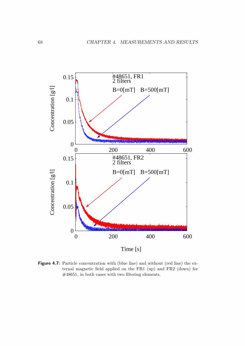
68 CHAPTER 4. MEASUREMENTS AND RESULTS
0
0.05
0.1
0.15
0 200 400 600
Con
cent
ratio
n [g
/l]
#48651, FR12 filters
B=0[mT] B=500[mT]
0
0.05
0.1
0.15
0 200 400 600
Con
cent
ratio
n [g
/l]
Time [s]
#48651, FR22 filters
B=0[mT] B=500[mT]
Figure 4.7: Particle concentration with (blue line) and without (red line) the ex-ternal magnetic field applied on the FR1 (up) and FR2 (down) for#48651, in both cases with two filtering elements.

4.2. NUMERICAL VALUES 69
Figure 4.4-4.7 shows the result of such fitting to the values measured duringthe filtering phase for the two different powders (for one and two filteringelements)7. For both powders a neat improvement in the retention efficiencyis visible when the magnetic field is applied. That improvement is morevisible with #48100, because the smaller particles are harder to capturewith sieving only. An improvement is also visible, for each powder, whentwo filtering elements are inserted instead of one.
4.2 Numerical values
In order to deduce numerical values from the former qualitative analysisthe mass balance model is applied (see Section 2.2). The fitting, performedfor each experiment separately, followed this algorithm:
1. the flow rate was determined in order to fit the frequency of the oscil-lations in the first phase of the calibration8;
2. the initial concentration was adjusted in order to reach the initial am-plitude;
3. the decay rates for population I and for population III were fitted inorder to follow the calibration phase slope9;
4. the decay rate for population II was fitted in order to follow the filtra-tion phase slope.
The results of such process is shown for some cases in Fig. 4.8 and in Fig.4.9 for #48100 and #48651 respectively10. It’s worth to note the differentbehaviour of the two turbidity meters: in FR2 data a neat peak is visible inthe filtering phase due to the clean water initially filling the filter. This par-ticular behaviour is well reproduced by the model too. The work performedon each set of measures led to the average values listed in Table 4.1 for onefiltering element and in Table 4.2 for two filtering elements. The resultsshow that, as expected, the capture is better with the magnetic field appliedand with two filtering elements. Table 4.3 shows the capture efficiencies ofthe filter in the various experimental conditions calculated from the results
7The time, equal for each figure and ranging from 0sec to 600sec, is calculated fromthe second starting of the pump.
8This is well visible in the left frame of Fig. 4.8 and 4.9.9This is visible in the right frame of Fig. 4.8 and 4.9 in which the initial values are
comparable to the experimental ones.10The time is rescaled starting from the first starting of the pump.

70 CHAPTER 4. MEASUREMENTS AND RESULTS
0 0.05
0.1 0.15
0.2 0.25
0.3 0.35
0.4 0.45
0 200 400 600 800 1000 1200 1400
Con
cent
ratio
n [g
/l]
#48100, FR1B=500[mT]
0.15
0.2
0.25
0 50 100
0.05 0.1
0.15
700 750
0
0.05
0.1
0.15
0.2
0.25
0.3
0.35
0.4
0.45
0 200 400 600 800 1000 1200 1400
Con
cent
ratio
n [g
/l]
Time [s]
#48100, FR2B=500[mT]
0.15
0.2
0.25
0 50 100
0.05 0.1
0.15
700 750
Figure 4.8: Experimental (thick lines) and simulated (thin lines) particle concen-tration with the external magnetic field applied on the FR1 (red) andFR2 (blue) for #48100.

4.2. NUMERICAL VALUES 71
0 0.05 0.1
0.15 0.2
0.25 0.3
0.35 0.4
0.45
0 200 400 600 800 1000 1200
Con
cent
ratio
n [g
/l]
#48651, FR1B=500[mT]
0.15
0.2
0.25
0 50 100 0.05
0.1
0.15
700 750
0
0.05
0.1
0.15
0.2
0.25
0.3
0.35
0.4
0.45
0 200 400 600 800 1000 1200
Con
cent
ratio
n [g
/l]
Time [s]
#48651, FR2B=500[mT]
0.15
0.2
0.25
0 50 100 0.05
0.1
0.15
700 750
Figure 4.9: Experimental (thick lines) and simulated (thin lines) particle concen-tration with the external magnetic field applied on the FR1 (red) andFR2 (blue) for #48651.

72 CHAPTER 4. MEASUREMENTS AND RESULTS
Table 4.1: Range of values used for the simulations with one filtering element,relative error of 10%.
#48100 #486511 filter 1 filter
Q[
m3/s]
0.11 × 10⁻³ 0.17 × 10⁻³
λ1,I
[
s−1]
0.22 × 10⁻³ 0.28 × 10⁻³
λ2,I
[
s−1]
(B = 0T) 0.20 0.30λ2,I
[
s−1]
(B = 500mT) 0.34 0.50λ3,I
[
s−1]
0.22 × 10⁻³ 0.28 × 10⁻³
λ1,II
[
s−1]
0.10 × 10⁻³ 0.40 × 10⁻³
λ2,II
[
s−1]
(B = 0T) 0.01 0.02λ2,II
[
s−1]
(B = 500mT) 0.02 0.03λ3,II
[
s−1]
0.10 × 10⁻³ 0.40 × 10⁻³
λ1,III
[
s−1]
1.10 × 10⁻³ 3.40 × 10⁻³
λ2,III
[
s−1]
(B = 0T) 0.12 0.08λ2,III
[
s−1]
(B = 500mT) 0.27 0.03λ3,III
[
s−1]
1.10 × 10⁻³ 3.40 × 10⁻³
mI [g] 0.20 0.18mII [g] 0.04 0.04mIII [g] 0.25 0.19
Data refers to experiments repeated at least two times.
of the system mass balance model using (2.33). The experimental activitywith two filtering elements has been carried out also as a further check ofthe separation results. In fact, the relation between the capture efficiency onone and two filtering elements in known by definition to be:
1 − σ2filters = (1 − σ1filter)2 (4.1)
Equation (4.1) is correct if the two filters are identical. In the present expe-rience conditions two different, i.e. hand made, filters have been used andthis circumstance led to an unavoidably slightly big experimental error.To check the deduced decay rates λi,k with the σ deduced from the cellmodel a number of cells between 6 and 8 for each filtering element has beenassumed. This number is due to the knowledge of the dept of the iron steelwool used in the construction of the filtring elements. The same knowledgelead to the value of the packaging factor Γ = 3.5 × 10⁻³. The capture ef-ficiency for the single cell is then estimated from eq.(2.28) as 0.1 ± 10%.This value must be compared with the results shown in Fig. 2.6. Assum-ing dp = 0.8 ± 20% µm, χp = 2 × 10⁻³ [Oka+02], µ0M = 1 T [BCD03],B0 = 0.5 T, η = 1 mPa·s, u0 = 0.15 m/s and rc = 15 µm I can deduce thecapture parameter Ω = 0.008±50%. This huge variation is not an error, buttakes into account the different sizes of the two particulate matters used. The

4.2. NUMERICAL VALUES 73
Table 4.2: Range of values used for the simulations with two filtering elements,relative error of 10%.
#48100 #486512 filters 2 filters
Q[
m3/s]
0.12 × 10⁻³ 0.17 × 10⁻³
λ1,I
[
s−1]
0.22 × 10⁻³ 0.35 × 10⁻³
λ2,I
[
s−1]
(B = 0T) 0.19 0.70λ2,I
[
s−1]
(B = 500mT) 0.50 1.00λ3,I
[
s−1]
0.22 × 10⁻³ 0.35 × 10⁻³
λ1,II
[
s−1]
0.11 × 10⁻³ 0.42 × 10⁻³
λ2,II
[
s−1]
(B = 0T) 0.02 0.03λ2,II
[
s−1]
(B = 500mT) 0.03 0.03λ3,II
[
s−1]
0.11 × 10⁻³ 0.42 × 10⁻³
λ1,III
[
s−1]
0.12 × 10⁻³ 0.40 × 10⁻³
λ2,III
[
s−1]
(B = 0T) 0.21 0.32λ2,III
[
s−1]
(B = 500mT) 0.42 0.42λ3,III
[
s−1]
0.12 × 10⁻³ 0.40 × 10⁻³
mI [g] 0.23 0.18mII [g] 0.05 0.04mIII [g] 0.24 0.22
Table 4.3: Capture efficiency in the various experimental conditions.
#48100 #48100 #48651 #486511 filters 2 filters 1 filters 2 filters
σfilter 0.25 ± 10% 0.35 ± 10% 0.4 ± 10% 0.7 ± 10%σ∗
filter 0.4 ± 10% 0.55 ± 10% 0.45 ± 10% 0.8 ± 10%∗ These values refer to the applied field case.
stronger limiting value of Ω deduced from (2.25) and (2.26) is 0.003 ± 50%.This limit is not that relevant since the capture efficiencies with and withoutparticles inertia, shown in Fig. 2.6, are nearly the same and quite constantin the considered range. Thus I deduce σcell = 0.09±10% from Fig. 2.6, thatis consistent with the one obtained with the system mass balance model. Itcan be seen from Table 4.3 and also from Fig. 4.4-4.7 that the improvementof the capture efficiency due to the application of the field is particularlymarked for #48100 probably thanks to the lower size of that powder withrespect to the #48651. On the other side, it is worth to note that, evenwithout external magnetic field applied, also the quasi-static model predictsa non zero number of stopped particles due to the fact that there are flowlines arbitrarily close to each fiber. Thus, in the limit case of a wool withinter-fibers distance always lower than the particles’ diameter each particle is

74 CHAPTER 4. MEASUREMENTS AND RESULTS
stopped. This confirms the applicability of the model to both the consideredexperimental conditions for each powder. For both powders a test withoutwool, i.e. with applied field only, gives no capture at all, as expected.

Chapter 5
Conclusions
After a short review of the state of the art in the magnetic separationfield a numerical model to simulate the capture process in an HGMS filteris presented. The model is aimed to improve the usual approaches to theproblem, which neglect the matrix to matrix interaction and oversimplifiesthe velocity and flux density fields. The proposed approach divides the filterinto a large number of elementary volumes (cells) and assume a spatial pe-riodicity condition. For a given cell geometry the velocity and flux densityfields resulting from the complete interaction of all the fibers of the wool areevaluated. This leads us to calculate the capture efficiency using a statis-tical approach both for the geometry of the cell and the trajectories of theparticles. An independent model is presented which describes the temporaryevolution of the particle concentration in the whole filter on the base of sim-ple assumption on the conservation of the particle number. With this secondmodel the check of the cell model to the experimental data is made possible.An experimental activity on a laboratory device has been carried out in orderto perform the test. An experimental facility has been projected and realizedin the LIMSA laboratory overcoming the quest of a REAL-time measuringset-up.The capture efficiencies for the cell obtained from the trajectory model arewell comparable and consistent with the experimental data. Moreover, theresults show that the filter efficiency is increased when the magnetic fieldis applied also for relatively small fields. This confirms the feasibility of theHGMS technology when SC magnets are utilized, but also opens the possibil-ity to utilize permanent magnets evaluating the trade off between efficiencyand cost. In order to scale the filter for an industrial process there is theneed to join the cell model with the system model taking into account thelocal conditions of the single cells such as relative orientation among woolfibers, external induction field and mean velocity field. It is also necessary to
75

76 CHAPTER 5. CONCLUSIONS
implement a model for the filter saturation making the capture efficiency atime dependent function. The problem of the dispose of the filtering elementhas been overcome using non-toxic iron oxide, but remains as an industrialtrial would start. The iron steel wool is very cheap so a disposal of the wholefiltering element remains possible. Conversely also its cleaning is available.The cleaning is possible with decreasing oscillating field in order to demag-netize the wool followed by a strong stream of air or liquid in order to drainaway the clogging.

Appendix A
Magnetization
A.1 Limiting magnetization of a spherical par-
ticle
To verify that the maximum magnetization for a spherical particle cannot exceed 3 we consider a sphere S of radius R immersed in an external anduniform magnetic field He directed along the z axis. We call the magneticpermeability of the sphere and of the medium, respectively, µp and µf . FromMaxwell equations we have, everywhere in space, ∇×H = 0 and ∇·B = 0, onthe discontinuity surfaces Ht|δS = continuos and Bn|δS = continuos and, atinfinity, H|∞ = He. Being the magnetic field conservative we can introducethe scalar potential ψ; distinguishing the region inside the sphere (in) and theouter one (out) we have Hin = −∇ψin and Hout = −∇ψout. Moreover, beingthe two materials homogeneous, the Laplace equation is satisfied in bothdomains: ∇2ψin = 0 and ∇2ψout = 0. We search the solution in sphericalcoordinates, with the polar axis along z. Being the inner field uniform whilethe outer the superposition of the external one and of the dipole one producedby the sphere we have:
ψin = −αHer sin θ ⇒ Hin = αHe(sin θer + cos θeθ)
= αHeez = αHe
ψout = −Her sin θ + βHeR3
r2sin θ ⇒ Hout = He + 2βHe
R3
r3sin θer
− βHeR3
r3cos θeθ
77
78 APPENDIX A. MAGNETIZATION
Thank to the polar symmetry we can write the interface conditions in thefollowing form:
Hin,θ(r = R) = Hout,θ(r = R) ⇒ α = 1 − β
µpHin,θ(r = R) = µfHout,θ(r = R) ⇒ αµp = µf + µf2β
Introducing the susceptibility µk = µ0(1 + χk) with k = p, f we achieve:
α =3 + 3χf
3 + χp + 2χfβ =
χp − χf
3 + χp + 2χf(A.1)
As stated the magnetic field inside the sphere is uniform. Moreover themagnetization is correlated to He with an affective susceptibility which isdifferent from the one of the material:
M = χpHin = χpαHe = χp,effHe (A.2)
in which we defined:
χp,eff = χp3 + 3χf
3 + χp + 2χf
(A.3)
We can notice that when χf = 0, i.e. the sphere is surrounded by air:
limχp<<1
χp,eff = χp
limχp>>1
χp,eff = 3
q.e.d..
A.2 Measures of magnetic permeability
An experimental facility has been realized in order to measure the mag-netic permeability of samples of magnetite powder1 and of iron steel wool.The relation between the sample magnetization and the material magneti-zation has been deduced in two different situation: considering a macro-scopically isotropic material and considering a macroscopically non isotropicone.
1The magnetic permeability of the hematite powder, being a paramagnetic substance,resulted beyond the experimental limit of the described instruments.

A.2. MEASURES OF MAGNETIC PERMEABILITY 79
A.2.1 Macroscopically isotropic material
Considering a mixture of linear phases with different magnetic perme-ability it’s possible to define B = µH everywhere. Anyway this function iscertainly quickly varying. Following Landau [LL87] the volumetric averageoperator can be introduced as follow:
< ψ >=1
V
∫
V
ψdτ
so that < B >= µmix < H >. Considering the mixture filling the spaceeverywhere, the average values of the fields result independent of the positionand defining the following local relations:
H =< H > +δH
µ =< µ > +δµ
Noting that, by definition:
< δH > = 0
< δµ > = 0
it’s possible to write:
< B >=< µH >=< µ >< H > + < δµδH > (A.4)
On the first order approximation µmix ≈< µ > +O ((δµ)2). To improve thisresult I consider now ∇ ·B = 0:
0 = ∇ · [µH] ≈< µ > ∇ · δH+ < H > ·∇δµ (A.5)
Being the mixture almost homogeneous:
∂
∂xδHx ≈ ∂
∂yδHy ≈ ∂
∂zδHz ≈ 1
3∇ · δH
and choosing the x axis along the H axis eq. (A.5) transform as
3 < µ >∂
∂xδHx+ < Hx >
∂
∂xδµ ≈ 0
which can be easily integrated independently of the x direction leading to:
δH ≈ − < H >
3 < µ >δµ

80 APPENDIX A. MAGNETIZATION
from which < δµδH >≈ − <H>3<µ>
< (δµ)2 > and the mixture permeability canbe well approximated by:
µmix ≈< µ > −< (δµ)2 >
3 < µ >(A.6)
For the sake of simplicity it is possible to search a relation of the formf(µmix) =< f(µ) >:
f(µmix) ≈ f
(
< µ > −< (δµ)2 >
3 < µ >
)
≈ f(< µ >) − < (δµ)2 >
3 < µ >f ′(< µ >)
< f(µ) > = 〈f(< µ > +δµ)〉 ≈
≈⟨
f(< µ >) + f ′(< µ >)δµ+1
2f ′′(< µ >)(δµ)2
⟩
=
= f(< µ >) +1
2f ′′(< µ >)
⟨
(δµ)2⟩
from which1
2f ′′(< µ >) = −f
′(< µ >)
3 < µ >
that can be easily integrated leading to, apart an addictive constant,f(< µ >) ∝< µ >
13 so that it’s possible to write:
µ13mix ≈
⟨
µ13
⟩
(A.7)
For example, for a mixture of spheres of susceptibility µs, in air and with avolume ratio of ζ = Vspheres/Vmix, it can be written:
µmix =[
ζµ13s + (1 − ζ)µ
130
]3
that satisfy the following properties:
1. ζ = 0 ⇒ µmix = µ0
2. ζ = 1 ⇒ µmix = µs
3. µs = µ0 ⇒ µmix = µ0, ∀ζ
4. µ0 ≤ µmix ≤ µs, ∀ζ, ∀µs ≥ µ0

A.2. MEASURES OF MAGNETIC PERMEABILITY 81
A.2.2 Macroscopically non isotropic material
If the considered mixture has a preferred orientation and the magneti-zation is isotropic orthogonally to that preferred orientation (such as if fer-romagnetic wool packet with the fibers mainly disposed along one directionis considered) some of the previous results can be still applied. Pointingthe preferred axis with the subscript ‖ and the orthogonal direction (justone symbol thanks to isotropy) with the subscript ⊥ it is possible to writeH = H‖ + H⊥ so that < B >= µmix,‖ < H‖ > +µmix,⊥ < H⊥ >. It followsthat, by definition:
< B > =< µ(H‖ + H⊥) >=
=< µH‖ > + < µH⊥ > + < δµδH‖ > + < δµδH⊥ >
Following the procedure of the previous section, from ∇ · B = 0 eq. (A.5)is obtained. Let follow previous section again : considering Hk ≡ H ≡ H⊥
(being k the versor along the z axis) implies
∂
∂xδHx ≈ ∂
∂yδHy ≈ 1
2∇ · δH, ∂
∂zδHz ≈ 0
so that:
δH⊥ ≈ −< H⊥ >
2 < µ >δµ
while considering H ≡ H‖ implies:
∂
∂xδHx ≈ ∂
∂yδHy ≈ 0,
∂
∂zδHz ≈ ∇ · δH
so that:
δH‖ ≈ −< H‖ >
< µ >δµ
From these results, substituting:
µmix,‖ ≈< µ > −< (δµ)2 >
< µ >, µmix,⊥ ≈< µ > −< (δµ)2 >
2 < µ >(A.8)
Moreover, searching for a relation of the form f(µmix) =< f(µ) > leads to:
f ′′⊥(< µ >) = −f
′⊥(< µ >)
< µ >, f ′′
‖ (< µ >) = −2f ′‖(< µ >)
< µ >
which have the following solutions:
f⊥(< µ >) ∝ ln < µ >, f‖(< µ >) ∝ 1/ < µ >

82 APPENDIX A. MAGNETIZATION
that is to say:
lnµmix,⊥
µ0
≈⟨
lnµ
µ0
⟩
,1
µmix,‖
≈⟨
1
µ
⟩
Considering iron steel wool, in air and with a ratio ζ = VFe/Vwool, it easilyfollows:
µwool,⊥
µ0
≈(
µFe
µ0
)ζ
,1
µmix,‖
≈ ζ
µFe+
1 − ζ
µ0
A.2.3 Measure of permeability
The facility aimed to the measures of susceptibility is visible in Fig. A.1.It mainly consists of a thin solenoid and a dynamometer: the field insidethe solenoid2, measured with the Gauss probe described in Section 3.1 andfitted with gnuplot via eq. (A.9) as visible in Fig. A.2, exerts a force3 ona specimen. That force, measured with the dynamometer, is visible in Fig.A.3a and Fig. A.3b for the magnetite and for the wool respectively. Usinggnuplot it is also possible to fit eq. (A.10), the analytical expression of theforce, with the experimental measures, as visible, again, in Fig. A.3a and Fig.A.3b. The effective susceptibility of the specimen, as described in AppendixA.1, is related to the traditional susceptibility which turns out to be relatedto the permeability of the mixture by:
µ = µ0(1 + χ) = µ0µr
For the magnetite, with ζ ≈ 0.76, a value χmagnetite,eff = 1.45 ± 0.05 wasmeasured which led to µmagtetite,eff ≈ 3.8×10⁻⁶H/m, that is µmagnetite,eff,r ≈3. The calculation with the wool data, with ζ ≈ 0.08, led to χwool,eff =0.61±0.02 which led to µwool,eff ≈ 2×10⁻⁶H/m, that is µAISI434L ≈ 500H/m
2The field inside a solenoid is expressed by eq. (A.9) as a known function of somegeometrical parameters and of the current in the wire [Sol]:
Be(z) =µ0nI
2
[
d + 2z√
(d + 2z)2 + 4r2+
d − 2z√
(d − 2z)2 + 4r2
]
(A.9)
n is the number of coils per meters, I is the current intensity, r is the inner radius of thesolenoid and d its thickness.
3The magnetic force acting on a spherical mixture of volume Vp with magnetic suscep-tibility χmix,eff in the main symmetry axis z of a solenoid due to the field Be expressedby eq. (A.9) is:
Fz =Vpχmix,eff
2µ0
∂
∂zB2
e,z (A.10)

A.2. MEASURES OF MAGNETIC PERMEABILITY 83
Figure A.1: Experimental set-up able to measure the magnetic force exerted on asample.
4. The value of magnetic permeability for the AISI 434 steel of the woolhas been compared, with a good agreement, with the value in [BCD03]. Acomparison for the magnetite powder resulted beyond the experimental and,moreover, the available data limits.
4The values of ζ for both samples were deduced form their volume and weight.

84 APPENDIX A. MAGNETIZATION
0.02
0.03
0.04
0.05
0.06
0.07
0.08
0.09
0.1
-0.02 0 0.02 0.04 0.06 0.08 0.1
B[T
]
z[m]
Figure A.2: Experimental field (dots) and its analytical expression fitted withgnuplot (continuous curve).

A.2. MEASURES OF MAGNETIC PERMEABILITY 85
0
0.02
0.04
0.06
0.08
0.1
0.12
0.14
-0.01 0 0.01 0.02 0.03 0.04 0.05
F[T
]
z[m](a) Experimental force on the magnetite sample (dots) and its analytical
expression fitted with gnuplot (continuous curve).
-0.01
0
0.01
0.02
0.03
0.04
0.05
0.06
-0.01 0 0.01 0.02 0.03 0.04 0.05
F[T
]
z[m](b) Experimental force on the wool sample (dots) and its analytical ex-
pression fitted with gnuplot (continuous curve).
Figure A.3: Experimental and analytical forces for the two samples.

86 APPENDIX A. MAGNETIZATION

Appendix B
Adsorption
B.1 Chemical reactions involved in the ad-
sorption process
This work is addressed to the remotion of pollutants from wastewatersthrough their bound in iron oxide. This adsorption process is a well estab-lished one both for magnetite and for hematite. When magnetite acquiresa metal it takes the name of spinel MFe2O4 where M = Ni(II), Co(II),Zn(II), Mg(II); when hematite acquires a rare hearth it takes the nameof orthoferrites MFeO3 where M = Gd(III), Sm(III). A typical way toexpress this relation for the magnetite is the following:
Fe2+ + Fe3+ + Fe3+ + 8OH− → FeOFeFeO3(solid) + 4H20
Fe2+ + M3+ + Fe3+ + 8OH− → FeOMFeO3(solid) + 4H20
M2+ + Fe3+ + Fe3+ + 8OH− → MFeOFeO3(solid) + 4H20
where FeOFe2O3 = Fe3O4 is the chemical formula of the magnetite. Fastand efficient adsorption of the divalent metals Zn, Co, Ni, and Cd tohematite is reported in literature [Jeo+04; Mam+09; Jeo+03]. The sorp-tion experiments for this iron oxide show that it is effective also for As(V ),Se(IV ), and Se(V I) at room temperature, and is rather independent fromthe concentration [Mam+09; Gim+07; Rov+08]. Moreover, as expected, theability to adsorb heavy metals is determined by the specific surface areas[BGE00]. This kind of reaction is well known and often used in various fields(not only in the inorganic separation one, but also, for example, in drugsdelivering and biochemical separation) [Gu+95; Gos+02; PDS09; HW82;Han07; Amb+03]. The reactions transform a solution with heavy metals andiron into a solution of heavy metals bounded in iron oxides without the need
87

88 APPENDIX B. ADSORPTION
of any external energy, provided that the environmental conditions (PH andtemperature of the working fluid) are suitable [SMK02].

Appendix C
Concentration
C.1 Particle distribution
As stated in Chapter 2 the particle size distribution is well describedby the superposition of three log-normal distribution [Logb]. A log-normaldistribution (normalized to K) is written as:
Ψ(ζ, µ, σ) =K
ζσ√
2πe−
(ln ζ−µ)2
2σ2 (C.1)
A fitting of the parameters of a first distribution ΨI for the magnetite distri-bution shown in Fig. C.1, made using gnuplot [Gnub], leads to the following
0
1
2
3
4
5
6
7
8
1 10 100
Freq
uenc
y %
Diameter [µm]
#48800
Figure C.1: Experimental size distributions for the magnetite powder (#48800).
89

90 APPENDIX C. CONCENTRATION
0
1
2
3
4
5
6
7
8
1 10 100
Freq
uenc
y %
Diameter [µm]
#48800ΨI
Figure C.2: Experimental size distributions for the magnetite powder confrontedwith the primary distribution.
parameters:
KI = 77.648743
µI = 2.041052
σI = 0.713806
As visible in Fig. C.2 two queues are visible. The fitting of the differencebetween the data and the first distribution with a second distribution ΨII
leads to:
KII = 20.941135
µII = 3.538794
σII = 0.277457
which corresponds to Fig. C.3. To consider the third queue too (the oneconcerning the smallest particles) another distribution ΨIII is fitted in thesame way obtaining:
KIII = 1.410121
µIII = −1.015040
σIII = 0.346363
which correctly describe the real particle distribution in the range of inter-est, as visible in Fig. C.4. The former procedure may be applied for the

C.1. PARTICLE DISTRIBUTION 91
0
1
2
3
4
5
6
7
8
1 10 100
Freq
uenc
y %
Diameter [µm]
#48800ΨI+ΨII
Figure C.3: Experimental size distributions for the magnetite powder confrontedwith the primary and a secondary distributions.
0
1
2
3
4
5
6
7
8
1 10 100
Freq
uenc
y %
Diameter [µm]
#48800ΨI+ΨII+ΨIII
Figure C.4: Experimental size distributions for the magnetite powder confrontedwith three log-normal distribution..
other particles (#48100 and #48651) with similar results. In Table C.1 thegeometric mean ζ and the geometric standard deviation of the mean ∇ζ forthe obtained distributions average size are highlighted [Loga]:
ζ = eµ
∇ζ = eσ

92 APPENDIX C. CONCENTRATION
Table C.1: Mean and standard deviation for the three populations (average size).
Population ζ[µm] ∇ζ[µm]
I 7.7 2.0II 34.5 1.3III 0.35 1.4
C.2 Model of the concentration vs resistance
relation.
Having a reliable description of the distribution of the size of the particlesleads to the relation that bounds the measured resistance on the photo-resistor to the particle concentration in the fluid (Chapter 3). As stated bythe maker of the photo-resistor [Nor] the following relation subsists betweenresistance R and incident light intensity I:
log
(
R
R#
)
= −β log
(
I
I#
)
(C.2)
where the subscript # stands for “normalization constant”. Supposing theattenuation of the light intensity through a length ds proportional to the par-ticle concentration (c(dp), where dp stands for the particle diameter) througha constant η plus a constant η0, the variation in the intensity of light can bewritten as:
dI = −[∫ ∞
0
d(dp)ηπd2
p
4c(dp) + η0
]
I · ds
This equation can be integrated from 0 to S leading to:
log
(
I
I0
)
= −Sπη4
∫ ∞
0
d(dp)d2pc(dp) − Sη0
where S is the length of the path travelled by the light (in the specific situ-ation the diameter of the pipe). Considering now, for the sake of simplicity,only particles with the same diameter:
c(dp) = C · δ(dp − d∗p)
where δ stands for the Dirac’s distribution, the previous equation can bewritten as:
log
(
I
I0
)
= −Sπη4d∗p
2C − Sη0

C.3. MEASURE FOR SAMPLES 93
Substituting this equation in eq. C.2 the following one is obtained:
log
(
R
R#
)
= −β
−Sπη4d∗p
2C − Sη0 + log
(
I0I#
)
from which it can be easily extracted the desired relation between resistanceand concentration:
C = a+ b logR (C.3)
where
a =4
πβηSd∗p2
βSη0 − β log
(
I0I#
)
− logR#
b =4
πβηSd∗p2
q.e.d..
C.3 Measure of concentration for samples of
working fluid
A concentration meter (Fig. C.5) has been realized for the measure ofsamples of the working water with the same components of the ones de-scribed in Section 3.3. These samples were collected into test-tubes and themeasured values compared with a scale of resistances as functions of time forknown concentrations, as the one in Fig. C.6, for the desired powder andrange of concentration. Every scale (for each powder and range of concen-trations) has been realized with ten tubes uniformly distributed in the rangeof interest. The initial concentrations in the tubes were made uniform withthe homemade mixer visible in Fig. C.7. A numerical model for depositionof the mixture of particles and bubbles in the tube arising from the mixinghas been developed in order to check the behaviour of Fig. C.6 and justifythe assumption of the existence of such a scale. I start from the equationfor a spherical particle1 with given diameter dp, density ρp in a fluid withdynamic viscosity µ and density ρf subjected to the gravity acceleration g,in a mono-dimensional reference system along the x-axis:
4π
3
(
dp
2
)2
ρpdv
dt=
4π
3
(
dp
2
)2
(ρp − ρf)g − 3πdpµv (C.4)
1The equation for the bubbles are formally identical, but their density is negligible.

94 APPENDIX C. CONCENTRATION
Figure C.5: Picture of the test-tube concentration-meter. The led lamp (powered)is on the right side of the tube while the photo-resistor is on the leftside. In the upper right corner a hat used to avoid the environmentallight modifying the measured value is visible. In the center-left is vis-ible R0 and in the right the contact board from National Instrument.
Introducing the time constant
τ =ρpd
2p
18µ
eq. (C.4) becomes:
dv
dt=ρp − ρf
ρpg − v
τ
which can be easily integrated obtaining
v(t) =ρp − ρf
ρpgτ(
1 − e−t/τ)

C.3. MEASURE FOR SAMPLES 95
100
1000
10000
100000
0 200 400 600 800 1000 1200 1400 1600
Res
ista
nce
[Ω
]
Time [sec]
C=1.0g/lC=0.9g/lC=0.8g/lC=0.7g/lC=0.6g/lC=0.5g/lC=0.4g/lC=0.3g/lC=0.2g/lC=0.1g/l
Figure C.6: Resistances as function of time for a set of tubes with given concen-tration of #48100 powder in water.
Neglecting the 5τ transient (which, in the considered experimental condi-tions, results of about 50µs) a further integration gives:
x = x(t; x0, dp) = x0 −ρp − ρf
ρpgτt = x0 − gτpt (C.5)
where
τp =(ρp − ρf )d
2p
18µ
Now assume that the particles are falling in a tube of length L and cross sec-tion A. The concentration c(x, t; dp) of identical particles of a given diameterdp, defined as number of particles of a given diameter dp per unit volume, inthe interval 0 < x < L, is given by:
c(x, t; dp) =
∫ L
0
dx0c0(dp)δ(x− x(t; x0, dp)) (C.6)
where δ is the Dirac distribution and the initial concentration is assumed tobe uniform, i.e. independent from x0. Note the sedimentation in x = 0 is

96 APPENDIX C. CONCENTRATION
Figure C.7: Homemade mixer used to guarantee initial uniform concentration inthe test-tubes.
not taken into account. Substitution and integration leads to:
c(x, t; dp) =
∫ L
0
dx0c0(dp)δ(x− x0 + gτpt) =
= c0(dp)
∫ ∞
0
dx0δ(x− x0 + gτpt) − c0(dp)
∫ ∞
L
dx0δ(x− x0 + gτpt) =
= c0(dp)[U(x+ gτpt) − U(x− L+ gτpt)]
where U is the Heaviside step function. Note that, in the interval 0 < x < L,this equals
c(x, t; dp) = c0(dp)[1 − U(x− L+ gτpt)]
The same is true for the bubbles. Neglecting their emersion, in the interval0 < x < L, we get:
cb(x, t; db) = cb,0(db)U(x− gτbt)
Now I define the distribution function f(dp) defining f(dp)d(dp) as number ofparticles of diameter between dp and dp + d(dp) divided by the total number

C.3. MEASURE FOR SAMPLES 97
of particles. Thus:∫ ∞
0
d(dp)f(dp) = 1
and the cumulative Φ(dp) =∫ dp
0d(dp)f(dp) is bounded, i.e. 0 < Φ < 1. The
same is true for the bubbles which have their distribution function fb(db) andtheir cumulative Φb.
Defining the total initial uniform concentration C0 as the total numberof particles and bubbles divided by the tube volume AL, the partial initialuniform concentration of particles is c0(dp) = Cp,0f(dp). The same is truefor the bubble concentration cb,0(db) = Cb,0fb(db). The total concentration ofparticles and bubbles at a given time and quote is given by
C(x, t) =
∫ ∞
0
d(dp)c(x, t; dp) +
∫ ∞
0
d(db)cb(x, t; db)
Substitution and integration leads to:
C(x, t) =
∫ ∞
0
d(dp)Cp,0f(dp)[1 − U(x− L+ gτpt) +
∫ ∞
0
d(db)Cb,0fb(db)U(x− gτbt)
= Cp,0
[∫ ∞
0
d(dp)f(dp) −∫ ∞
0
d(dp)f(dp)U(x − L+ gτpt)
]
+ Cb,0
∫ ∞
0
d(db)fb(db)U(x− gτbt)
This function can be integrated and studied, as in Appendix C.2, substitutingthe log-normal distribution for the particle diameter. This leads to a relationof the form:
R = a′ + b′log(C) (C.7)
which justifies the scaling hypothesis.

98 APPENDIX C. CONCENTRATION
C.4 Details of the components of the turbid-
ity meters
This appendix shows some details of the elements constituting the twoturbidity meters.
Figures C.8-C.9 show the schematics of the led and of the light-dependentresistor, respectively. All the values are in inches.
Figure C.8: Technical scheme of the led (lengths are in inches) [Led].

C.4. DETAILS OF THE COMPONENTS 99
Figure C.9: Technical scheme of the light dependent resistor (lengths are in inches)[Nor].

100 APPENDIX C. CONCENTRATION
Figures C.10a-C.10b show the frequency response of the light-dependentresistor and of the led, respectively. As visible both have a maximum around6KHz, i.e. green light, and consequently are well comparable.
(a) Light adsorption as function of its frequency [Nor].
(b) Intensity of the light emission as function of its frequency [Led].
Figure C.10: Frequency compatibility of the two elements.

Bibliography
[AA02] T. Abbasov and A. S. Altunbas. “Determination of the particlecapture radius in magnetic filters with velocity distribution pro-file in pores”. In: Separation Science and Technology 37.9 (June2002), pp. 2037–2053.
[ACA05] P. A. Augusto, T. Castelo-Grande, and P. Augusto. “Magneticclassification in health sciences and in chemical engineering”. In:Chemical Engineering Journal 111.2-3 (Aug. 2005), pp. 85–90.issn: 1385-8947. doi: 10.1016/j.cej.2005.02.013.
[Adl+67] A. D. Adler et al. “A simplified synthesis for meso-tetraphenylporphine”. In: The Journal of Organic Chemistry32.2 (Feb. 1967), p. 476. doi: 10.1021/jo01288a053.
[AKH99] T. Abbasov, M. Koksal, and S. Herdem. “Theory of high-gradient magnetic filter performance”. In: Magnetics, IEEETransactions on 35.4 (1999), pp. 2128–2132. issn: 0018-9464.
[ALM03] M. Ahoranta, J. Lehtonen, and R. Mikkonen. “Magnet de-sign for superconducting open gradient magnetic separator”.In: Physica C 386 (2003), pp. 398–402.
[Amb+03] R. D. Ambashta et al. “Nano-aggregates of hexacyanoferrate(II)-loaded magnetite for removal of cesium from radioactivewastes”. In: Journal of Magnetism and Magnetic Materials267.3 (Dec. 2003), pp. 335–340. issn: 0304-8853. doi: 10.1016/S0304-8853(03)00401-3.
[Ana02] G. N. Anastassakis. “Separation of Fine Mineral Particles by Se-lective Magnetic Coating”. In: Journal of Colloid and InterfaceScience 256 (2002), pp. 114–120.
[AP98] U. M. Ascher and L. R. Petzold. Computer Methods for Or-dinary Differential Equations and Differential-Algebraic Equa-tions. 1st ed. University City Science Center, Philadelphia: So-ciety for the Industrial and Applied Mathematics, 1998.
101

[Bar] Barometer. 2010. url: http://www.wika.de/.
[BB05] R. Bucher and S. Balemi. “Scilab/Scicos and Linux RTAI - aunified approach”. In: Control Applications, 2005. CCA 2005.Proceedings of 2005 IEEE Conference on. 2005, pp. 1121–1126.isbn: 1085-1992. doi: 10.1109/CCA.2005.1507281.
[BCD03] J. Bas, J. Calero, and M. Dougan. “Sintered soft magnetic ma-terials. Properties and applications”. In: Journal of Magnetismand Magnetic Materials 254-255 (2003), pp. 391–398.
[BCZ07] L. W. Bruch, M. W. Cole, and E. Zaremba. Physical Adsorp-tion: Forces and Phenomena. Dover Publications, 2007. isbn:0486457672.
[BGE00] J. P. Beukes, E. W. Giesekke, and W. Elliott. “Nickel retentionby goethite and hematite”. In: Minerals Engineering 13.14-15(Dec. 2000), pp. 1573–1579. issn: 0892-6875. doi: 10.1016/
S0892-6875(00)00140-0.
[Bir+78a] R. Birss et al. “Laminar flow model of particle capture of axialmagnetic filters”. In: Magnetics, IEEE Transactions on 14.6(1978), pp. 1165–1169. issn: 0018-9464.
[Bir+78b] R. Birss et al. “Theory and performance of axial magnetic filtersin laminar flow conditions”. In: Magnetics, IEEE Transactionson 14.5 (1978), pp. 389–391. issn: 0018-9464.
[BMD06] S. Babel and D. del Mundo Dacera. “Heavy metal removal fromcontaminated sludge for land application: A review”. In: WasteManagment 26 (2006), pp. 988–1004.
[BMN06] R. Bucher, S. Mannori, and T. Netter. RTAI-Lab tutorial:Scilab, Comedi, and real-time control. 2006. url: www.rtai.org/RTAILAB.
[BPS80] R. Birss, M. Parker, and T. Sheerer. “Statistics of particle cap-ture in HGMS”. In: Magnetics, IEEE Transactions on 16.5(1980), pp. 830–832. issn: 0018-9464.
[Bre97] M. Breschi. “Processi di cattura nei separatori magnetici super-conduttivi”. Thesys. University of Bologna, 1997.
[Bru+05] W. Bruckard et al. “Water leaching and magnetic separationfor decreasing the chloride level and upgradin the zinc contentof EAF steelmaking baghouse dust”. In: Int. J. Miner. Process.75 (2005), pp. 1–20.
102

[CBN98] A. Cristofolini, M. Breschi, and F. Negrini. “Capture processesin superconducting HGMS”. In: Proceedings of the 1998 In-ternational Symposium on Advanced Energy Technology (Feb.1998).
[Che98] N. P. Cheremisinoff. Liquid Filtration, Second Edition. 2nd ed.Butterworth-Heinemann, 1998. isbn: 0750670479.
[CKK76] C. Clarkson, D. Kelland, and T. King. “Model for calculation ofcapture radii of a high gradient magnetic separator at moderateReynolds numbers”. In: Magnetics, IEEE Transactions on 12.6(1976), pp. 901–903. issn: 0018-9464.
[CKT82] H. Collan, M. Kokkala, and O. Toikka. “Application of the the-ory of magnetic filtration in determining the optimum filter con-figuration”. In: Magnetics, IEEE Transactions on 18.3 (1982),pp. 827–832. issn: 0018-9464.
[Coe02] J. M. D. Coey. “Permanent magnet applications”. In: Jour-nal of Magnetism and Magnetic Materials 248.3 (Aug. 2002),pp. 441–456.
[EIA09] A. Eskandarpour, K. Iway, and S. Asai. “Superconducting mag-netic filter: performance, recovery and design”. In: IEEE Trans.on Appl. Supercond. 19.2 (2009), pp. 84–95.
[ERP97] A. D. Ebner, J. A. Ritter, and H. J. Ploehn. “Feasibilityand Limitations of Nanolevel High Gradient Magnetic Sepa-ration”. In: Separation and Purification Technology 11 (1997),pp. 199–210.
[Esk+07] A. Eskandarpour et al. “Semi-continuous Magnetic Removal ofPhosphate Using an Iron Oxide Hydroxide Adsorbent and Re-generation of Its Adsorbent”. In: ISIJ International 47.4 (2007),pp. 563–567.
[Fab+03a] M. Fabbri et al. “Infuence of the electro-magnetic stirring onthe boundary layer of a molten steel pool”. In: COMPEL 22.1(2003).
[Fab+03b] M. Fabbri et al. “Removal of SiC inclusions in molten aluminiumusing a 12 T static magnetic feld”. In: COMPEL 22.1 (2003).
[Fab08] M. Fabbri. “Magnetic flux density and vector potential of uni-form polyhedral sources”. In: IEEE Trans. Magn. 44.1 (Jan.2008), pp. 32–36.
103

[Fab+08] M. Fabbri et al. “High gradient magnetic separation ofmicro-pollutant from waste waters”. In: Proc. 1st EuropeanConference on Microfluidics (MicroFlu’08). Bologna 2008,pp. 270.1–270.13. isbn: 2-906831-76-X.
[Fab09] M. Fabbri. “Magnetic flux density and vector potential of linearpolyhedral sources”. In: COMPEL 28.6 (2009), pp. 1688–1700.
[Fle91] D. Fletcher. “Fine particle high gradient magnetic entrap-ment”. In: Magnetics, IEEE Transactions on 27.4 (1991),pp. 3655–3677. issn: 0018-9464.
[FS08] G. Fuchs and L. Schultz. “Encyclopedia of Materials: Scienceand Technology”. In: ed. by K. H. J. Buschow et al. ElsevierLtd., 2008. Chap. Superconducting Permanent Magnets: Prin-ciples and Results, pp. 8947–8955. isbn: 978-0-08-043152-9.
[FY05] G. Friedman and B. Yellen. “Magnetic separation, manipulationand assembly of solid phase in fluids”. In: Current Opinion inColloid Interface Science 10 (2005), pp. 158–166.
[Gar08] M. H. Garcia. Sedimentation Engineering: Theories, Measure-ments, Modeling and Practice: Processes, Management, Model-ing, and Practice. 1st ed. American Society of Civil Engineers,2008. isbn: 0784408149.
[GB83] R. Gerber and R. Birss. High Gradient Magnetic Separation.Research Studies Press, 1983.
[Gim+07] J. Gimenez et al. “Arsenic sorption onto natural hematite, mag-netite, and goethite”. In: Journal of Hazardous Materials 141.3(Mar. 2007), pp. 575–580. issn: 0304-3894. doi: 10.1016/j.jhazmat.2006.07.020.
[GL89] R. Gerber and P. Lawson. “The HGMS filter performance ex-ponential law”. In: Magnetics Conference, 1989. Digests of IN-TERMAG ’89., International. 1989, GD4.
[GMS88] R. Gregory, R. J. Maloney, and M. Stockley. “Water TreatmentUsing Magnetite: A Study of a Sirofloc Pilot Plant”. In: Waterand Environment Journal 2.5 (1988), pp. 532–544. doi: 10.
1111/j.1747-6593.1988.tb01335.x.
[Gmt] Iron steel wool. 2007. url: www.gmt-inc.com.
[Gnua] Copyright of gnuplot. 2010. url: http : / / gnuplot . cvs .
sourceforge.net/gnuplot/gnuplot/Copyright.
[Gnub] gnuplot. 2010. url: http://www.gnuplot.info/.
104

[Gol04] R. Goleman. “Macroscopic model of particles’ capture by theelliptic cross-section collector in magnetic separator”. In: Jour-nal of Magnetism and Magnetic Materials 272-276.Part 3 (May2004), pp. 2348–2349. issn: 0304-8853. doi: 10.1016/j.jmmm.2003.12.963.
[Gos+02] Y. Gossuin et al. “Cesium Adsorption in Hydrated Iron OxideParticles Suspensions: An NMR Study”. In: Journal of MagneticResonance 157.1 (July 2002), pp. 132–136. issn: 1090-7807. doi:10.1006/jmre.2002.2581.
[Gra01] J. Graham. Biological Centrifugation. 1st. Garland Science,2001. isbn: 1859960375.
[Gu+95] B. Gu et al. “Adsorption and desorption of different organicmatter fractions on iron oxide”. In: Geochimica et Cosmochim-ica Acta 59.2 (1995), pp. 219–229. issn: 0016-7037. doi: 10.1016/0016-7037(94)00282-Q.
[Ha+] D. Ha et al. “Treatment of Wastewater of Iron Manifacturingby Superconducting High Gradient Magnetic Separation”. In:().
[Han07] K. Hanna. “Sorption of two aromatic acids onto iron oxides:Experimental study and modeling”. In: Journal of Colloid andInterface Science 309.2 (May 2007), pp. 419–428. issn: 0021-9797. doi: 10.1016/j.jcis.2007.01.004.
[HBW82] B. L. Hirschbein, D. W. Brown, and G. M. Whitesides.“Magnetic separations in chemistry and biochemistry”. In:CHEMTECH 12.3 (1982), pp. 172–179.
[HKA00] S. Herdem, M. Koksal, and T. Abbasov. “Model for PredictingFiltration Efficiency and Pressure Drop in Axial Magnetic Fil-ters”. In: Separation Science and Technology 35.7 (2000), p. 941.issn: 0149-6395. doi: 10.1081/SS-100100203.
[HLG70] J. P. Herzig, D. M. Leclerc, and P. L. Goff. “Flow of Suspensionsthrough Porous Media Application to Deep Filtration”. In: In-dustrial & Engineering Chemistry 62.5 (May 1970), pp. 8–35.doi: 10.1021/ie50725a003.
[HNW76] J. Harland, L. Nilsson, and M. Wallin. “Pilot scale high gradi-ent magnetic filtration of steel mill wastewater”. In: Magnetics,IEEE Transactions on 12.6 (1976), pp. 904–906. issn: 0018-9464.
105

[Hos+05] M. A. Hossain et al. “Ineffectiveness and Poor Reliability of Ar-senic Removal Plants in West Bengal, India”. In: EnvironmentalScience & Technology 39.11 (June 2005), pp. 4300–4306. doi:10.1021/es048703u.
[HU80] K. Hayashi and S. Uchiyama. “On particle trajectory and cap-ture efficiency around many wires”. In: Magnetics, IEEE Trans-actions on 16.5 (Sept. 1980), pp. 827–829. issn: 0018-9464.
[Hub+01] J. J. Hubbuch et al. “High gradient magnetic separation ver-sus expanded bed adsorption: a first principle comparison”.In: Bioseparation 10.1 (2001), pp. 99–112. doi: 10.1023/A:1012034923621.
[HW82] B. L. Hirschbein and G. M. Whitesides. “Affinity separa-tion of enzymes from mixtures containing suspended solids”.In: Applied Biochemistry and Biotechnology 7.3 (May 1982),pp. 157–176. doi: 10.1007/BF02798294.
[Jeo+03] B. Jeon et al. “Sorption kinetics of Fe(II), Zn(II), Co(II), Ni(II),Cd(II), and Fe(II)/Me(II) onto hematite”. In: Water Research37.17 (Oct. 2003), pp. 4135–4142. issn: 0043-1354. doi: 10.
1016/S0043-1354(03)00342-7.
[Jeo+04] B. Jeon et al. “Modeling the sorption kinetics of divalentmetal ions to hematite”. In: Water Research 38.10 (May 2004),pp. 2499–2504. issn: 0043-1354. doi: 10.1016/j.watres.2004.03.003.
[JM06] M. W. Jornitz and T. H. Meltzer. Pharmaceutical Filtration:The Management of Organism Removal. PDA/DHI, 2006. isbn:193011477X.
[KAH03] M. Koksal, T. Abbasov, and S. Herdem. “Mathematical mod-eling of the magnetic filtration processes”. In: IOS Press 18.4(2003), pp. 227–234. issn: 1383-5416.
[Kak+04] Y. Kakihara et al. “Superconducting High Gradient MagneticSeparation for Purification of Wastewater From Paper Factory”.In: IEEE Trans. on Appl. Supercond. 14.2 (2004). Poco interes-sante.
[Kar03] N. Karapinar. “Magnetic separation of ferrihydrite fromwastewater by magnetic seeding and high-gradient magneticseparation”. In: Int. J. Miner. Process. 71 (2003), pp. 45–54.
106

[Kel73] D. Kelland. “High gradient magnetic separation applied to min-eral beneficiation”. In: Magnetics, IEEE Transactions on 9.3(1973), pp. 307–310. issn: 0018-9464.
[Kir00] V. A. Kirsh. “The Effect of van der Waals’ Forces on AerosolFiltration with Fibrous Filters”. In: Colloid Journal 62.6 (Nov.2000), pp. 714–720. doi: 10.1023/A:1026678725025.
[Kir04] V. Kirsh. “Inertial Deposition of Aerosol Particles on FiberousFilters”. In: Colloid Journal 66 (5 2004), pp. 613–618.
[KS77] A. Kirsch and I. Stechkina. “Inertial deposition of aerosol par-ticles in model filters at low reynolds numbers”. In: Journal ofAerosol Science 8.5 (Sept. 1977), pp. 301–307. issn: 0021-8502.doi: 10.1016/0021-8502(77)90016-7.
[Lat73] C. de Latour. “Magnetic separation in water pollution control”.In: Magnetics, IEEE Transactions on 9.3 (1973), pp. 314–316.issn: 0018-9464.
[LD75] F. Luborsky and B. Drummond. “High gradient magnetic sepa-ration: Theory versus experiment”. In: Magnetics, IEEE Trans-actions on 11.6 (1975), pp. 1696–1700. issn: 0018-9464.
[Led] High emission led. 2005. url: http://www.datasheetarchive.com/pdf/Datasheet-018/DSA00321875.pdf.
[Leu98] W. Leung. Industrial Centrifugation Technology. 1st ed.McGraw-Hill Professional, 1998. isbn: 0070371911.
[LK75] C. de Latour and H. Kolm. “Magnetic separation in water pol-lution control - II”. In: Magnetics, IEEE Transactions on 11.5(1975), pp. 1570–1572. issn: 0018-9464.
[LL06] L. Landau and E. Lifshitz. Fluid Mechanics. 2nd ed. Vol. 6.Course of Theoretical Physics. Elsevier, 2006.
[LL87] E. Lifshitz and L. Landau. Electrodynamics of continuous me-dia. 2nd ed. Vol. 8. Course of Theoretical Physics. PergamonPress, 1987.
[Loga] Log-normal distribution - Wikipedia. 2010. url: http://en.wikipedia.org/wiki/Log-normal distribution.
[Logb] Lognormal Distribution. 2010. url: http://www.itl.nist.gov/div898/handbook/eda/section3/eda3669.htm.
107

[Mam+09] Y. Mamindy-Pajany et al. “Arsenic adsorption onto hematiteand goethite”. In: Comptes Rendus Chimie 12.8 (Aug. 2009),pp. 876–881. issn: 1631-0748. doi: 10.1016/j.crci.2008.10.012.
[Mar+09a] G. Mariani et al. “High gradient magnetic separation of micro-pollutant from waste waters”. In: La Houille Blanche - Interna-tional Water Journal 6 (Dec. 2009). DOI: 10.1051/lhb/2009087,pp. 109–117.
[Mar+09b] G. Mariani et al. “High gradient magnetic separation of pol-lutant from wastewaters”. In: 8th International Symposium onElectric and Magnetic Fields (EMF 2009) Book of Summaries.Mondovi (Italy) 2009, pp. 79–80.
[Mar+10] G. Mariani et al. “High gradient magnetic separation of micro-pollutant from wastewaters using permanent magnets”. In: Sep-aration and Purification Technology (2010). In press.
[Mas+06] J. Masse et al. “Influence of relative density on the architectureand mechanical behaviour of a steel metallic wool”. In: ScriptaMaterialia 54.7 (Apr. 2006), pp. 1379–1383. issn: 1359-6462.doi: 10.1016/j.scriptamat.2005.11.075.
[May+07] J. Mayo et al. “The effect of nanocrystalline magnetite size onarsenic removal”. In: Science and Technology of Advanced Ma-terials 8.1-2 (2007), p. 71. url: http://iopscience.iop.org/1468-6996/8/1-2/A13.
[MBQ07] W. P. Martignoni, S. Bernardo, and C. L. Quintani. “Evaluationof cyclone geometry and its influence on performance parame-ters by computational fluid dynamics (CFD)”. en. In: BrazilianJournal of Chemical Engineering 24 (Mar. 2007), pp. 83 –94.issn: 0104-6632. url: http://www.scielo.br/scielo.php?script=sci arttext&pid=S0104-66322007000100008&nrm=
iso.
[McM02] J. E. McMurry. Fundamentals of Organic Chemistry. 5th ed.Brooks Cole, 2002. isbn: 0534395732.
[MHB05] C. Mikkelsen, M. F. Hansen, and H. Bruus. “Theoretical com-parison of magnetic and hydrodynamic interactions betweenmagnetically tagged particles in microfluidic systems”. In: Jour-nal of Magnetism and Magnetic Materials 293.1 (May 2005),pp. 578–583. issn: 0304-8853. doi: 10.1016/j.jmmm.2005.01.076.
108

[Mit+03] K. Mitsuhashi et al. “Purification of endocrine disrupter-polluted water using high temperature superconductingHGMS”. In: Physical Separation in Science and Engineering12.4 (2003), pp. 205–213.
[MK78] E. Maxwell and D. Kelland. “High gradient magnetic separationin coal desulfurization”. In: Magnetics, IEEE Transactions on14.5 (1978), pp. 482–487. issn: 0018-9464.
[Moe+04] G. D. Moeser et al. “High-gradient magnetic separation ofcoated magnetic nanoparticles”. In: AIChE Journal 50.11(2004), pp. 2835–2848. doi: 10.1002/aic.10270.
[MSG99] L. Morino, F. Salvatore, and M. Gennaretti. “A new velocitydecomposition for viscous flows: Lighthill’s equivalent sourcemethod revisited”. In: Comput. Methods Appi. Mech. Engrg.173 (1999), pp. 317–336.
[MW] A. D. McNaught and A. Wilkinson. Compendium of ChemicalTerminology. 1997th ed. Oxford: Blackwell Scientific Publica-tions. isbn: 0-9678550-9-8.
[Nak+03] H. Nakajima et al. “Separation characteristics of open gradientmagnetic separation using high-temperature superconductingmagnet”. In: Physica C: Superconductivity 392-396.Part 2 (Oct.2003), pp. 1214–1218. issn: 0921-4534. doi: 10.1016/S0921-4534(03)01128-6.
[Nat] Safe Drinking Water Is Essential. 2007. url: http : / /
drinking- water.org/html/en/Treatment/Coagulation-
Flocculation-technologies.html.
[Neg+99] F. Negrini et al. “A Multi wire Model for SuperconductingHGMS Filter”. In: Proc. Int. Conf. on MHD Power Genera-tion and High Temperature Technologies. Ed. by P. J. Zixiang.Vol. 2. Institute of Electrical Engineering of the Chinese Aca-deny of Sciences. Beijing, PRC Oct 1999 1999, pp. 715–720.
[Nor] Photo-resistor. 2007. url: http://www.alldatasheet.com/datasheet-pdf/pdf/124422/ETC/NORP12.html.
[NS03] J. D. Navratil and M. T. Shing-Tsair. “Magnetic separationof iron and heavy metals from water”. In: Water Science andTechnology: A Journal of the International Association on Wa-ter Pollution Research 47.1 (2003). PMID: 12578170, pp. 29–32.issn: 0273-1223.
109

[NT06] S. Nishijima and S. ichi Takeda. “Superconducting High Gradi-ent Magnetic Separation for Purification of Wastewater fromPaper Factory”. In: IEEE Trans. on Appl. Supercond. 16.2(2006), pp. 1142–1145.
[Obe+75] J. A. Oberteuffer et al. “High gradient magnetic filtration ofsteel mill process and waste waters”. In: Magnetics, IEEETransactions on 11.5 (1975), pp. 1591–1593. issn: 0018-9464.
[Obe76] J. A. Oberteuffer. “Engineering development of High Gradi-ent Magnetic Separators”. In: IEEE Trans. Magn. MAG-12.5(1976), pp. 444–449.
[Ode76] R. Oder. “High gradient magnetic separation theory and ap-plications”. In: Magnetics, IEEE Transactions on 12.5 (1976),pp. 428–435. issn: 0018-9464.
[Oka+02] H. Okada et al. “High gradient magnetic separation for weaklymagnetized fine particles”. In: IEEE Trans. on Appl. Supercond.12.1 (Mar. 2002), pp. 967–970.
[Oli+02] L. C. A. Oliveira et al. “Activated carbon/iron oxide magneticcomposites for the adsorption of contaminants in water”. In:Carbon 40.12 (2002), pp. 2177–2183. issn: 0008-6223. doi: 10.1016/S0008-6223(02)00076-3.
[OM05] H. Okada and K. Mitsuhashi. “Computational Fluid DynamicsSimulation of High Gradient Magnetic Separation”. In: Sepa-ration science and technology 7 (2005), pp. 1567–1584. issn:0149-6395.
[PDS09] A. Pathak, M. G. Dastidar, and T. R. Sreekrishnan. “Bioleach-ing of heavy metals from sewage sludge: A review”. In: Journalof Environmental Managment 90 (2009), pp. 2343–2353.
[Rho98] M. Rhodes. Introduction to Particle Technology. Wiley, 1998.isbn: 0471984833.
[Rov+08] M. Rovira et al. “Sorption of selenium(IV) and selenium(VI)onto natural iron oxides: Goethite and hematite”. In: Journalof Hazardous Materials 150.2 (2008), pp. 279–284. issn: 0304-3894. doi: 10.1016/j.jhazmat.2007.04.098.
[RW01] L. L. Regel and W. R. Wilcox. Processing by Centrifugation.1st ed. Springer, 2001. isbn: 0306466546.
[Sah+99] N. Saho et al. “Continuous Superconducting-Magnet FiltrationSystem”. In: IEEE Trans. on Appl. Supercond. 9.2 (1999).
110

[San88] A. V. Sandulyak. “Magnetic filtration of liquids and gases”. In:Ximya (1988). in Russian.
[SF03] H. Shen and E. Forssberg. “An overview of recovery of metalsfrom slags”. In: Waste Management 23.10 (2003), pp. 933–949.issn: 0956-053X. doi: 10.1016/S0956-053X(02)00164-2.
[Sha] H. H. Shalaby. “On the potential of large eddy simulation tosimulate cyclone separators”. In: url: http://archiv.tu-
chemnitz.de/pub/2007/0013/index.html.
[SK] J. L. Smith and J. H. Keenan. Experimental and an-alytical study of the vortex in the cyclone separator.http://dspace.mit.edu/handle/1721.1/11792. Thesis (Sc. D.)–Massachusetts Institute of Technology, Dept. of Mechanical En-gineering, 1959.
[SMK02] T. K. Sen, S. P. Mahajan, and K. C. Khilar. “Adsorption ofCu2+ and Ni2+ on iron oxide and kaolin and its importanceon Ni2+ transport in porous media”. In: Colloids and SurfacesA: Physicochemical and Engineering Aspects 211.1 (Nov. 2002),pp. 91–102. issn: 0927-7757. doi: 10.1016/S0927-7757(02)00235-2.
[SML04] R. Scanlan, A. Malozemoff, and D. Larbalestier. “Superconduct-ing materials for large scale applications”. In: Proceedings of theIEEE. Vol. 92. 10. 2004, pp. 1639–1654.
[Sol] Finite Solenoid. 2005. url: http://www.netdenizen.com/
emagnet/solenoids/solenoidonaxis.htm.
[Sto06] M. Stolarski. “Magnetic field enhanced press-filtration”. In:Chemical Engineering Science 61 (2006), pp. 6395–6403.
[Suh00] J. C. Suh. “The evaluation of the Biot-Savart integral”. In:J.Eng.Math. 37 (2000), pp. 375–395.
[Sut08] K. Sutherland. Filters and Filtration Handbook, Fifth Edition.5th ed. Elsevier Science, 2008. isbn: 1856174646.
[Svo87] J. Svoboda. Magnetic Methods for the Threatment of Minerals.Elsevier, 1987.
[Tar+03] P. Tartaj et al. “The preparation of magnetic nanoparticles forapplications in biomedicine”. In: Journal of Physics D: AppliedPhysics 36.13 (2003).
[Tar86] V. I Tarushkin. Electric separator for seed. Muhammad Ali So-ciety, 1986.
111

[Tas] “Treatment of Coolant of Hot Rolling Process by High GradientMagnetic Separation”. In: IEEE Trans. on Appl. Supercond.17.2 (2007), pp. 2189–2191.
[Tso+06] C. Tsouris et al. “Surfactant effects on the mechanism of particlecapture in high-gradient magnetic filtration”. In: Separation andPurification Technology 51 (2 2006), pp. 201–209.
[UAA03] T. Uslu, Atalay, and A. Arol. “Effect of microwave heatingon magnetic separation of pyrite”. In: Colloids and SurfacesA: Physicochemical and Engineering Aspects 225.1-3 (2003),pp. 161–167.
[Uch+76] S. Uchiyama et al. “Performance of parallel stream type mag-netic filter for HGMS”. In: Magnetics, IEEE Transactions on12.6 (Nov. 1976), pp. 895–897. issn: 0018-9464.
[Wat73] J. H. P. Watson. “Magnetic filtration”. In: Journal of AppliedPhysics 44.9 (1973), pp. 4209–4213. doi: 10.1063/1.1662920.
[Wat75] J. H. P. Watson. “Theory of capture of particles in magnetichigh-intensity filters”. In: Magnetics, IEEE Transactions on11.5 (1975), pp. 1597–1599. issn: 0018-9464.
[WB86] J. H. P. Watson and C. Boorman. “A Superconducting High-Gradient Magnetic Separator with a Current-carrying Ma-trix”. In: Internation Juornal of Mineral Processing 17 (1986),pp. 161–185.
[Wu+04] R. Wu et al. “Removal of azo-dye Acid Red B (ARB) by adsorp-tion and catalytic combustion using magnetic CuFe2O4 pow-der”. In: Applied Catalysis B: Environmental 48.1 (Mar. 2004),pp. 49–56. issn: 0926-3373. doi: 10.1016/j.apcatb.2003.09.006.
[Yav+06a] C. T. Yavuz et al. “Low-Field Magnetic Separation of Monodis-perse Fe3O4 Nanocrystals”. In: Science 314.5801 (Nov. 2006),pp. 964–967. doi: 10.1126/science.1131475.
[Yav+06b] H. Yavuz et al. “Biosorption of mercury on magnetically modi-fied yeast cells”. In: Separation and Purification Technology 52.2(2006), pp. 253–260.
[Yav+09] C. T. Yavuz et al. “Magnetic separations: From steel plants tobiotechnology”. In: Chemical Engineering Science 64.10 (May2009), pp. 2510–2521. issn: 0009-2509. doi: 10.1016/j.ces.2008.11.018.
112

[Yea+05] S. Yean et al. “Effect of magnetite particle size on adsorptionand desorption of arsenite and arsenate”. In: Journal of Mate-rials Research 20.12 (2005), pp. 3255–3264.
[You+06] D. Young et al. “Method of fundamental solutions for mul-tidimensional Stokes equations by the dual-potential formula-tion”. In: European Journal of Mechanics B/Fluids 25 (2006),pp. 877–893.
[YYT00] T. Y. Ying, S. Yiacoumi, and C. Tsouris. “High-gradient mag-netically seeded filtration”. In: Chemical Engineering Science55 (2000), pp. 1101–1113.
[Zha07] J. Zhang. “Composite magnetic microspheres: Preparation andcharacterization”. In: Journal of Magnetism and Magnetic Ma-terials 309 (2007), pp. 197–201.
Others (Italian)
[Fab+06a] M. Fabbri et al. “Analisi di sensitivita sui parametri del processodi magnetizzazione del campo intrappolato da magneti perma-nenti superconduttivi”. In: Atti della 22a Riunione annuale deiRicercatori di Elettrotecnica. ET2006. Torino 2006, pp. 1–2.
[Fab+06b] M. Fabbri et al. Studio sui trasformatori superconduttivi adalta temperatura critica. Rapporto Finale Contratto CESI-DIE/2006. Departiment of Electrical Engeneering, 2006.
[Mar+09c] G. Mariani et al. “Separazione magnetica dei microinquinantidalle acque reflue”. In: Atti della 25a Riunione annuale deiRicercatori di Elettrotecnica-ET2009. Lecce 2009, pp. 1–2.
[MFN07] G. Mariani, M. Fabbri, and F. Negrini. “Studio della separazionemagnetica dei microinquinanti prioritari dalle acque reflue”. In:Atti della 23a Riunione annuale dei Ricercatori di Elettrotec-nica. ET2007. Firenze 2007, pp. 1–2. url: http://www.cirlab.unifi.it/ET2007/memorie/098.pdf.
[MFN08] G. Mariani, M. Fabbri, and F. Negrini. “Studio della separazionemagnetica dei microinquinanti prioritari dalle acque reflue”. In:Atti della 24a Riunione annuale dei Ricercatori di Elettrotec-nica. ET2008. Pavia 2008, pp. 1–2.
113

Index of Cited Authors
Abbasov, T., 16–19, 21Adler, A. D., 5Ahoranta, M., 8Altunbas, A. S., 17Ambashta, R. D., 87Anastassakis, G. N., 7Arol, A. I., 22Asai, S., 11Ascher, U. M., 35Atalay, 22Augusto, P., 24Augusto, P. A., 24
Babel, S., 1Balemi, S., 53Bas, J.A., 37, 46, 72, 83Bernardo, S., 3Beukes, J. P., 87Birss, R., 16, 23Boorman, C.H., 25Breschi, M., 13Brown, D. W., 22Bruch, L. W., 6Bruckard, W.J., 11Bruus, H., 33Bucher, R., 53
Calero, J.A., 37, 46, 72, 83Castelo-Grande, T., 24Cheremisinoff, N. P., 2Clarkson, C., 14Coey, J. M. D., 11Cole, M. W., 6Collan, H., 19
Cristofolini, A., 13
Dastidar, M. G., 87Dougan, M.J., 37, 46, 72, 83Drummond, B., 15
Ebner, A. D., 11Elliott, W., 87Eskandarpour, A., 11, 13
Fabbri, M., 13, 28, 37, 47Fletcher, D., 20Forssberg, E., 23Friedman, G., 7Fuchs, G., 10
Garcia, M. H., 6Gennaretti, M., 29Gerber, R., 18, 23Giesekke, E. W., 87Gimenez, J., 87Goff, P. Le., 12Goleman, R., 15Gossuin, Y., 87Graham, J., 5Gregory, R., 23Gu, B., 87
Ha, Dong-Woo, 22Hanna, K., 87Hansen, M. F., 33Harland, J., 22Hayashi, K., 12, 16Herdem, S., 16–19, 21Herzig, J. P., 12
114

Hirschbein, B. L., 21, 22, 87Hossain, M. A., 23Hubbuch, J., 20
Iway, K., 11
Jornitz, M. W., 2
Kakihara, Y., 22Karapinar, N., 22Keenan, J. H., 4Kelland, D., 14, 22Khilar, K. C., 88King, T., 14Kirsch, A.A., 11Kirsh, V.A., 11Kirsh, V. A., 35Kokkala, M., 19Koksal, M., 16–19, 21Kolm, H., 23
Landau, L.D., 7, 31, 33, 56, 79Larbalestier, D.C., 10Latour, C. de, 23Lawson, P., 18Leclerc, D. M., 12Lehtonen, J., 8Leung, W., 5Lifshitz, E.M., 7, 31, 33, 56, 79Luborsky, F., 15
Mahajan, S. P., 88Maloney, R. J., 23Malozemoff, A.P., 10Mamindy-Pajany, Y., 87Mannori, S., 53Mariani, G., 26, 27, 59Martignoni, W. P., 3Masse, J.P., 46Maxwell, E., 22Mayo, J.T., 23McMurry, J. E., 6
McNaught, A. D., 5Meltzer, T. H., 2Mikkelsen, C., 33Mikkonen, R., 8Mitsuhashi, K., 20, 23, 25Moeser, G. D., 20Morino, L., 29Mundo D., D. del, 1
Nakajima, H., 8Navratil, J. D., 20Negrini, F., 10, 13Netter, T., 53Nilsson, L., 22Nishijima, S., 22
Oberteuffer, J. A., 7, 22, 25Oder, R., 21Okada, H., 20, 25, 37, 50, 72Oliveira, L. C. A., 25
Parker, M., 16Pathak, A., 87Petzold, L. R., 35Ploehn, H. J., 11
Quintani, C. L., 3
Regel, L. L., 5Rhodes, M., 3Ritter, J. A., 11Rovira, M., 87
Saho, N., 11Salvatore, F., 29Sandulyak, A. V., 17Scanlan, R.M., 10Schultz, L., 10Sen, T. K., 88Shalaby, H. H., 4Sheerer, T., 16Shen, H., 23Shing-Tsair, M. T., 20
115

Smith, J. L., 4Sreekrishnan, T. R., 87Stechkina, I.B., 11Stockley, M., 23Stolarski, M., 3Suh, J. C., 28, 30, 32Sutherland, K., 3Svoboda, J., 7
Takeda, S. ichi, 22Tartaj, P., 24Tarushkin, V. I, 6Toikka, O., 19Tsouris, C., 35
Uchiyama, S., 12, 16Uslu, T., 22
Wallin, M., 22Watson, J. H. P., 7, 12, 13, 25Whitesides, G. M., 21, 22, 87Wilcox, W. R., 5Wilkinson, A., 5Wu, R., 24
Yavuz, C. T., 11, 21, 23, 24Yavuz, H., 23, 24Yean, S., 23Yellen, B., 7Yiacoumi, S., 35Ying, T. Y., 35Young, D.L., 29
Zaremba, E., 6Zhang, Ji, 21
116


![3 U arXiv:1111.1528v2 [cond-mat.str-el] 14 May 2012juser.fz-juelich.de/record/127401/files/1111.1528.pdf · the prototypical Jahn-Teller magnetic perovskite LaMnO3 at different levels](https://static.fdocuments.us/doc/165x107/6082ddb3460e8809083eebc0/3-u-arxiv11111528v2-cond-matstr-el-14-may-the-prototypical-jahn-teller-magnetic.jpg)