Theoretical and experimental study of particle...

Phil. Trans. R. Soc. A (2012) 370, 1543–1571doi:10.1098/rsta.2011.0446

Theoretical and experimental study of particletrajectories for nonlinear water waves

propagating on a sloping bottomBY YANG-YIH CHEN1,2, MENG-SYUE LI1, HUNG-CHU HSU3,* AND

CHIU-ON NG4

1Department of Marine Environment and Engineering, National Sun Yat-senUniversity, Kaohsiung 80424, Taiwan

2Department of Hydraulic and Ocean Engineering, National Cheng KungUniversity, Tainan 70955, Taiwan

3Tainan Hydraulics Laboratory, National Cheng Kung University,Tainan 70101, Taiwan

4Department of Mechanical Engineering, The University of Hong Kong,Hong Kong, People’s Republic of China

A third-order asymptotic solution in Lagrangian description for nonlinear water wavespropagating over a sloping beach is derived. The particle trajectories are obtained asa function of the nonlinear ordering parameter 3 and the bottom slope a to the thirdorder of perturbation. A new relationship between the wave velocity and the motionsof particles at the free surface profile in the waves propagating on the sloping bottom isalso determined directly in the complete Lagrangian framework. This solution enables thedescription of wave shoaling in the direction of wave propagation from deep to shallowwater, as well as the successive deformation of wave profiles and water particle trajectoriesprior to breaking. A series of experiments are conducted to investigate the particletrajectories of nonlinear water waves propagating over a sloping bottom. It is shownthat the present third-order asymptotic solution agrees very well with the experiments.

Keywords: Lagrangian; sloping bottom; particle trajectory; wave velocity relation;wave breaking

1. Introduction

In the process of a wave propagating from deep to shallow water, the wavewill deform and eventually break. The wave changes in height and its profilebecomes asymmetrical during the process of shoaling. In this connection, manyresearchers have paid much attention to solving the wave transformation onsloping bottoms. Moreover, it is also very important for the tsunami issue asdiscussed by Segur [1] and Constantin & Johnson [2]. However, since the slopingbottom was approximated by a large number of steps, the effects of the bottom*Author for correspondence ([email protected]).

One contribution of 13 to a Theme Issue ‘Nonlinear water waves’.

This journal is © 2012 The Royal Society1543

on July 14, 2018http://rsta.royalsocietypublishing.org/Downloaded from

mailto:[email protected]

http://rsta.royalsocietypublishing.org/

1544 Y.-Y. Chen et al.

slope could not be fully explained in many models. Biesel [3] suggested a plausibleapproximation method to account for the normal incident waves propagatingon a sloping plane where the bottom slope was first considered in the velocitypotential as a perturbation parameter. Chen & Tang [4] modified Biesel’s [3]theoretical model and obtained a linear solution to the first order of the bottomslope. For nonlinear waves on a beach, Carrier & Greenspan [5] gave an analyticalsolution for the shallow water wave motion of finite-amplitude, non-breakingwaves on a beach of constant slope. Chu & Mei [6] and Liu & Dingemans [7]presented perturbation solutions for weakly nonlinear waves propagating overan uneven bottom. Chen et al. [8] derived a fourth-order asymptotic solution ofnonlinear water waves propagating normally towards a mild beach. Chen et al.[8] used the transformation from Eulerian to Lagrangian coordinates to calculatethe water particle motion up to the second order, by which the profile of ashoaling wave sequence until the breaking point can be evaluated. However, astraightforward expansion of the Eulerian solution of Stokes waves up to the thirdorder cannot be transformed into the corresponding Lagrangian solution. Chen &Hsu [9] presented a modified Euler–Lagrange transformation method to obtainthe third-order trajectory solution in a Lagrangian form for the water particles innonlinear water waves. Unlike an Eulerian surface, which is given as an implicitfunction, a Lagrangian form is expressed through a parametric representation ofparticle motion. Hence, the Lagrangian description is more appropriate for thefree surface motion, whereas this unique feature cannot be represented by theclassical Eulerian solutions [3,8,10–17].

The first water wave theory in Lagrangian coordinates was obtained byGerstner [18] who assumed the flow possesses non-constant vorticity in infinitedepth. Miche [19] proposed a perturbation method for Lagrangian solution to thesecond order for a gravity wave motion. Pierson [20] also applied perturbationexpansion to water wave problems with Lagrangian formulae and obtained afirst-order Lagrangian solution. Buldakov et al. [16] developed a Lagrangianasymptotic formulation up to the fifth order for nonlinear water waves in deepwater. Recently, for travelling waves in irrotational flow over a flat bed, the generalfeatures of the particle paths have been obtained without the assumption of smallamplitude (necessary for a power-series approach) by Constantin [21]; the particletrajectories in solitary water waves have also been obtained by Constantin &Escher [22]; and Constantin & Strauss [23] have extended the work to describethe pressure beneath a Stokes wave. Additionally, Constantin & Escher [24] havefurther exposed the analyticity of periodic travelling free surface water waves withvorticity. Chen & Hsu [9] obtained a third-order solution for irrotational finiteamplitude standing waves in Lagrangian coordinates. The particle path is similarto Ehrnström & Wahlen [25]. Hsu et al. [26] derived a Lagrangian asymptoticsolution up to the second order for short-crested waves. Asymptotic solutionsup to the fifth order which describe irrotational finite amplitude progressivegravity water waves were recently derived in Lagrangian description by Chen etal. [27]. All the theories mentioned above are limited to the condition of uniformwater depth. To date, only a few analytical solutions have been derived forwave transformation on a planar beach in Lagrangian coordinates. Among them,Sanderson [28] obtained a second-order solution in a uniformly stratified fluidwith a small bottom slope in a Lagrangian system. Constantin [29] consideredthe Lagrangian solution for edge waves on a sloping beach. Chen & Huang [30]

Phil. Trans. R. Soc. A (2012)



Particle trajectories for water waves 1545

Cw (wave velocity)

= tan bd

db

Hbh(x,t)

(x)

x

y

ab

o

Figure 1. Definition sketch for surface-wave propagation on a uniformly sloping bottom.

derived a linear Lagrangian solution in terms of beach slope a to the second orderfor a progressive wave propagating over a gentle plane slope, while Kapinski [31]studied the run-up of a long wave over a uniform sloping bottom in Lagrangiandescription.

The purpose of this paper is to develop a nonlinear solution for surface wavespropagating over a sloping bottom in a Lagrangian description and to comparethe theory with a series of experiments. In order to examine the effect of a slopingbottom and wave steepness on surface waves, a perturbation expansion is usedto derive an expression for the particle trajectories in terms of wave steepness 3and the bottom slope a to the third power. The asymptotic solutions for physicalquantities related to the wave motion are then obtained up to the third order.Finally, to validate the accuracy of the analytical results, a series of laboratoryexperiments are performed. The Lagrangian properties of particle trajectories areshown to agree with the experimental data very well.

2. Formulation of the problem

Consider a two-dimensional monochromatic wave propagating on a uniform gentleslope without refraction as shown in figure 1. The negative x-axis is outward tothe sea from the still water level (SWL) shoreline, while the y-axis is taken positivevertically upward from the SWL, and the sea bottom is at y = −d = ax0, in whicha denotes the bottom slope.

The fluid motion in the Lagrangian representation is described by keepingtrack of individual fluid particles. For two-dimensional flow, a fluid particle isidentified by the horizontal and vertical parameters (x0, y0) known as Lagrangianlabels. Then fluid motion is described by a set of trajectories x(x0, y0, t) andy(x0, y0, t), where x and y are the Cartesian coordinates. The dependent variablesx and y denote the position of any particle at time t and are functions of theindependent variables x0, y0 and t. In a system of Lagrangian description, thegoverning equations and boundary conditions for two-dimensional irrotationalfree-surface flow are summarized as follows:

J = v(x , y)v(x0, y0)

= xx0yy0 − xy0yx0 = 1, (2.1)

xx0tyy0 − xy0tyx0 + xx0yy0t − xy0yx0t = v(xt , y)v(x0, y0)

+ v(x , yt)v(x0, y0)

= 0, (2.2)

xx0txy0 − xy0txx0 + yx0tyy0 − yy0tyx0 = v(xt , x)v(x0, y0)

+ v(yt , y)v(x0, y0)

= 0, (2.3)





vf

vx0= xtxx0 + ytyx0 ,

vf

vy0= xtxy0 + ytyy0 (2.4)

andPr

= −vf

vt− gy + 1

2(x2

t + y2t ). (2.5)

In equations (2.1)–(2.5), subscripts x0, y0 and t denote partial differentiationwith respect to the specified variable, P(x0, y0, t) is water pressure and f(x0, y0, t)is a velocity potential function in Lagrangian system. Except for equations(2.4) and (2.5) by Chen [32], the fundamental physical relationships definingthe equations above have been derived previously [19,20,33,34]. Equation(2.1) is the continuity equation that sets the invariant condition on thevolume of a Lagrangian particle and y0 = 0 is the vertical label marked fora particle at free surface; equation (2.2) is the differentiation of equation(2.1) with respect to time. Equations (2.3) and (2.4) govern the irrotationalflow condition and define the corresponding Lagrangian velocity potential,respectively. Equation (2.5) is the Bernoulli equation for irrotational flow inLagrangian description.

The wave motion has to satisfy a number of boundary conditions at the bottomand on the free water surface.

— On an immovable and impermeable sloping plane with an inclination tothe horizon, the no-flux bottom boundary condition gives

yt − axt = 0 and y = y0 = −d = ax0. (2.6)

— The dynamic boundary condition of zero pressure at the free surface is

P = 0, y0 = 0. (2.7)

— A time-averaged and stationary mass flux conservation condition isrequired: as waves propagate towards the beach, a horizontal hydrostaticpressure gradient to balance the radiation stress of the progressive wavewill produce a return flow and a boundary condition should be imposed.The additional condition usually employed is the condition of time-averaged mass flux conservation. This condition is necessary for theuniqueness of the solution and requires that at any cross section of thex–y plane, the time-averaged mass flux should vanish [8,35,36]

y direction :1T

∫T

0

∫ 0

−dv dy0 dt = 1

T

∫T

0

∫ 0

−dyt dy0 dt = 0 (2.8)

x direction :1T

∫T

0

∫ 0

−du dy0 dt = 1

T

∫T

0

∫ 0

−dxt dy0 dt

− U (a)T

∫T

0

∫ 0

−d0

xct dy0 dt =

∫ 0

−du dy0

− U (a)∫ 0

−d0

uc dy0 = 0, U (a) ={0, a �= 0,1, a = 0.

(2.9)





Both the superscript c and the subscript 0 express the physical quantity atx → −∞. Because of the nonlinear effect, waves over constant depth induce anet flux of water. Thus, a constant depth streaming term is introduced in (2.9)which is adjusted by a unit function U (a) to ensure that it can be reduced to theconstant depth condition when the bottom slope is equal to zero.

3. Asymptotic solutions

To solve equations (2.1)–(2.9), it is assumed that relevant physical quantitiescan be expanded as a double power series in terms of the bottom slope a andnonlinear parameter 3. Thus, the particle displacements x and y, the potentialfunction f, wave pressure P, wavenumber k and Lagrangian wave frequency scan be obtained as the following:

x = x0 +∞∑

m=0

∞∑n=0

3man[fm,n(x0, y0, st) + f ′m,n(x0, y0, s0,0t)]

= x0 +∞∑

m=0

∞∑n=0

3man[Am,n,iFm,n,i(S) + A′m,n,iF

′m,n,i(S)], (3.1)

y = y0 +∞∑

m=0

∞∑n=0

3man[gm,n(x0, y0, st) + g ′m,n(x0, y0, s0,0t)]

= y0 +∞∑

m=0

∞∑n=0

3man[Bm,n,iGm,n,i(S) + B ′m,n,iG

′m,n,i(S)], (3.2)

f =∞∑

m=0

∞∑n=0

3man[

fm,n(x0, y0, st) + f′m,n(s0,0t) +

∫Mm,n,0(x0, s0,0t)dx0

]

=∞∑

m=0

∞∑n=0

3man[

fm,n,iFm,n,i(S) + f′m,n(s0,0t) +

∫Mm,n,0(x0, s0,0t)dx0

],

(3.3)

P = −rgy0 +∞∑

m=0

∞∑n=0

3manPm,n(x0, y0, st), (3.4)

k =∞∑

m=0

∞∑n=0

3mankm,n(x0, y0) (3.5)

and s =∞∑

m=0

3mansm,n(x0, y0), (3.6)

where S is the phase function S = ∫k dx0 − st, x(x0, y0, t) and y(x0, y0, t) are

the particle displacements and the Lagrangian variable (x0, y0) are any twocharacteristic parameters, 3 is the nonlinear ordering parameter characterizing thewave steepness and Mm,n,0 is the return flow. s = 2p/T is the angular frequency ofthe particle motion or the Lagrangian angular frequency for a particle reappearing





at the same phase, where T is the period of particle motion. For a relativelygentle bottom slope a, it may be assumed that the q-th differentiations of Am,n,i ,A′

m,n,i , Bm,n,i , B ′m,n,i , fm,n,i , Mm,n,0 and km,n with respect to x0 are in the order

of aq : (dqkm,n

dxq0

,vqMm,n,0

vxq0

,dqAm,n,i

dxq0

,dqA′

m,n,i

dxq0

,dqBm,n,i

dxq0

,dqB ′

m,n,i

dxq0

,dqfm,n,i

dxq0

)= O(aq), q, n ∈ 0, 1, 2, . . . N . (3.7)

Substituting equations (3.1)–(3.6) into equations (2.1)–(2.9) and collecting theterms of the like order in 3 and a, we obtain the necessary equations to eachorder of approximation. Then different orders of 3(m), a(n) and harmonic (i)may be separated, yielding a set of partial differential equations for each index(m, n, i). Following these assumptions, analytical solutions for the problem underconsideration can then be obtained.

(a) 31a0-order approximation

Upon collecting terms of order 31a0, the governing equations of the conti-nuity equation, irrotational flow condition and Bernoulli equation can beexpressed as

(f1,0x0 + f ′1,0y0

) + (g1,0y0 + g ′1,0y0

) + [s0,0x0(f1,0t1 + f ′1,0t0)

+ s0,0y0(g1,0t1 + g ′1,0t0)]t = 0, (3.8a)

s0,0[(f1,0x0t1 + f ′1,0x0t0) + (g1,0y0t1 + g ′

1,0y0t0)]+ [s0,0x0(f1,0t1 + f ′

1,0t0) + s0,0y0(g1,0t1 + g ′1,0t0)]

+ s0,0[s0,0x0(f1,0t21+ f ′

1,0t20) + s0,0y0(g1,0t2

1+ g ′

1,0t20)]t = 0, (3.8b)

s0,0[(f1,0y0t1 + f ′1,0y0t0) − (g1,0x0t1 + g ′

1,0x0t0)]+ [s0,0y0(f1,0t1 + f ′

1,0t0) − s0,0x0(g1,0t1 + g ′1,0t0)]

+ s0,0[s0,0y0(f1,0t21+ f ′

1,0t20) − s0,0x0(g1,0t21

+ g ′1,0t20

)]t = 0, (3.8c)

f1,0x0 + f′1,0x0

+ s0,0x0t(f1,0t1 + f′1,0t0) + M1,0,0 = s0,0(f1,0t1 + f ′

1,0t0), (3.8d)

f1,0y0 + f′1,0y0

+ s0,0y0t(f1,0t1 + f′1,0t0) = s0,0(g1,0t1 + g ′

1,0t0) (3.8e)

andP1,0

r= −s0,0(f1,0t1 + f′

1,0t0) − g(g1,0 + g ′1,0) − gy0. (3.8f )

The condition for zero pressure at the free surface is

P1,0 = 0 and y0 = 0, (3.8g)

while the bottom boundary condition is

g1,0t1 + g ′1,0t0 = 0 and y = y0 = −d (3.8h)





and time-averaged and stationary mass flux conservation conditions in x- andy-direction are

1T

∫T

0

∫ 0

−ds0,0(g1,0t1 + g ′

1,0t0) dy0 dt = 0 (3.8i)

and

1T

∫T

0

∫ 0

−ds0,0(f1,0t1 + f ′

1,0t0) dy0 dt − 1T

∫T

0

∫ 0

−d0

s0,0(f c1,0t1 + f ′c

1,0t0) dy0 dt = 0. (3.8j)

The solutions for equations (3.8a)–(3.8j) can be easily obtained as

f1,0 = A1,0,1(x0) cosh k0,0(y0 + d) sin S ,

g1,0 = B1,0,1(x0) sinh k0,0(y0 + d) cos S ,

A1,0,1 = −B1,0,1, f ′1,0 = g ′

1,0 = s0,0a = s0,0b = f′1,0 = 0,

f1,0 = −s0,0

k0,0A1,0,1(x0) cosh k0,0(y0 + d) sin S ,

P1,0

r= −gy0 + gA1,0,1(x0)

sinh k0,0y0

cosh k0,0dcos S

and s20,0 = gk0,0 tanh k0,0d.

⎫⎪⎪⎪⎪⎪⎪⎪⎪⎪⎪⎪⎪⎪⎪⎬⎪⎪⎪⎪⎪⎪⎪⎪⎪⎪⎪⎪⎪⎪⎭

(3.9)

It is obvious that the solutions are not affected by the sloping bottom at this order.

(b) 31a1-order approximation

To the next order in O(31a1), the governing equations are given by

[A1,0,1x0 cosh k0,0(y0 + d) + A1,0,1k0,0x0(y0 + d) sinh k0,0(y0 + d)

+ A1,0,1k0,0dx0 sinh k0,0(y0 + d)] sin S + ak0,1A1,0,1 cosh k0,0(y0 + d) cos S

+ a[−A1,1,1k0,0 sin S + B1,1,1y0 sin S ] = 0, (3.10a)

− s0,0[A1,0,1x0 cosh k0,0(y0 + d) + A1,0,1k0,0x0(y0 + d) sinh k0,0(y0 + d)

+ A1,0,1k0,0dx0 sinh k0,0(y0 + d)] cos S + as0,0k0,1A1,0,1 cosh k0,0(y0 + d)

× sin S + as0,0[A1,1,1k0,0 cos S − B1,1,1y0 cos S ] = 0, (3.10b)

− s0,0[B1,0,1x0 sinh k0,0(y0 + d) + B1,0,1k0,0x0(y0 + d) cosh k0,0(y0 + d)

+ B1,0,1k0,0dx0 cosh k0,0(y0 + d)] sin S + as0,0k0,1B1,0,1 sinh k0,0(y0 + d)

× cos S + as0,0[−B1,1,1k0,0 sin S + A1,1,1y0 sin S ] = 0, (3.10c)

[f1,0,1x0 sin S + ak0,1f1,0,1 cos S − ak0,0f1,1,1 sin S + M1,1,0]= as0,0A1,1,1 sin S , (3.10d)





af1,1,1y0 cos S = −as0,0B1,1,1 cos S (3.10e)

and aP1,1

r= −as0,0f1,1,1 sin S − gaB1,1,1 sin S , (3.10f )

and the boundary conditions at the free surface and the bottom are

P1,1 = 0, y0 = 0 (3.10g)

and

s0,0a[−B1,1,1 cos S + A1,0,1 cosh k0,0(y0 + d) cos S ] = 0, y = y0 = −d. (3.10h)

A general solution for A1,1,1 and B1,1,1, which satisfies both continuity equationand irrotational flow condition, can be assumed as

aA1,1,1 = [M12(y0 + d)2 + M11(y0 + d) + M10] cosh k0,0(y0 + d)

+ [N11(y0 + d) + N10] sinh k0,0(y0 + d)(3.11)

and

aB1,1,1 = [M12(y0 + d)2 + M11(y0 + d) + M10] sinh k0,0(y0 + d)

+ [N11(y0 + d) + N10] cosh k0,0(y0 + d).(3.12)

Substituting equations (3.11) and (3.12) into equations (3.10a), (3.10b) and(3.10c) and omitting the secular term, the complex constants M1n and N1n arefound to be

M12 = 12B1,0,1k0,0x0 , M11 =B1,0,1k0,0dx0 , M10 = aB1,0,1

D2 tanh k0,0d, D = 1+ 2k0,0d

sinh 2k0,0d

and N12 = 0, N11 = B1,0,1x0 , N10 = aA1,0,1, k0,1 = M1,1,0 = 0.

⎫⎪⎬⎪⎭

(3.13)

Further substituting equation (3.13) into equation (3.10e) and using the freesurface boundary condition, equation (3.10g), we can obtain

B1,0,1 = asinh k0,0d

, a = a0√k0,0d sech2 k0,0d + tanh k0,0d

= aoKs, (3.14)

where a0 is the amplitude of the incident waves in deep water and a is that onthe sloping bottom; a0 and a are related as follows:

a = a0√D tanh k0d

= aoKs, (3.15)

where parameter Ks is the conventional shoaling coefficient. Based on the solu-tions derived, let us briefly discuss the effect of bottom slope on the free surfacedisplacement y(x0, y0 = 0, t). First, the correction to the free surface displacementat O(31a1) is 90◦ out of phase with respect to the leading order solution (31a0).





Second, the wave amplitude is enhanced and the phase is modified owing to theeffect of the slope. The solutions of 31a1 are completely determined as

A1,1,1 = B1,0,1

{[k20,0(y0 + d)2

D sinh 2k0,0d− k0,0(y0 + d) + 1

D2 tanh k0,0d

]cosh k0,0(y0 + d)

+[

k0,0(y0 + d)D2 tanh k0,0d

+ 2k0,0(y0 + d)D sinh 2k0,0d

− 1]

sinh k0,0(y0 + d)

},

B1,1,1 = B1,0,1

{[k20,0(y0 + d)2

D sinh 2k0,0d− k0,0(y0 + d) + 1

D2 tanh k0,0d

]sinh k0,0(y0 + d)

+[

k0,0(y0 + d)D2 tanh k0,0d

+ 2k0,0(y0 + d)D sinh 2k0,0d

− 1]

cosh k0,0(y0 + d)

},

f1,1,1 = −s0,0

k0,0B1,0,1

{[k20,0(y0 + d)2

D sinh 2k0,0d− k0,0(y0 + d)

]cosh k0,0(y0 + d)

+ k0,0(y0 + d)D2 tanh k0,0d

sinh k0,0(y0 + d)

},

P1,1

r= −[s0,0f1,1,1 + gB1,0,1] sin S

and k0,1 = s0,1 = 0.

⎫⎪⎪⎪⎪⎪⎪⎪⎪⎪⎪⎪⎪⎪⎪⎪⎪⎪⎪⎪⎪⎪⎪⎪⎪⎪⎪⎪⎪⎪⎪⎪⎪⎪⎪⎪⎪⎬⎪⎪⎪⎪⎪⎪⎪⎪⎪⎪⎪⎪⎪⎪⎪⎪⎪⎪⎪⎪⎪⎪⎪⎪⎪⎪⎪⎪⎪⎪⎪⎪⎪⎪⎪⎪⎭

(3.16)

The parametric functions for the water particle at any position in Lagrangiancoordinates (x , y) up to the 31a1 order are given as

(x − x0)2

(B1,0,1 cosh(k0,0(b + d)))2 + (aA1,1,1)2+ (y − y0)2

(B1,0,1 sinh(k0,0(b + d)))2 + (aB1,1,1)2= 1.

(3.17)

Figure 2 shows the trajectories up to 31a1 order of a progressive wave over asloping bottom; the orbital shape is clearly varying with the depth. The angle bbetween its main axis and the horizontal axis can also be calculated by coordinatetransformation. Neglecting terms of orders higher than O(32a0), the inclinationb can be given by

tan b = −a

[k0,0(y0 + d)

D2 tanh k0,0d+ 2k0,0(y0 + d)

D sinh 2k0,0d− 1

]. (3.18)

In equation (3.18), tan b increases as the water depth d decreases. It eventuallyapproaches a maximum (tan b = a) at bottom y0 = −d, where the slope of themain axis coincides with the slope along the direction of a wave ray over thesloping bottom. This implies that a water particle moves along the bottomsurface. Figure 2 also shows that the inclination b of a water particle trajectoryincreases with the decrease in water depth (k ′

0,0d) and bottom slope.





0.8(a)

(b)

(d)

(c)

(e)

( f ) (g)

0.4

0

–0.4

–0.8–8 –7 –6

0.2

0.2

–0.2

–0.2

–0.4

–0.4

–0.6–4.9 –4.7 –4.5 –4.3 –4.1

0

0.2 0.2

–0.2

–0.4

0

–0.2

–0.4–2.9 –2.7 –2.5 –2.3 –2.1 –2.4 –2.2 –2.0 –1.8 –1.6

0

–0.2

–0.4

–0.6

–0.8–7.9 –7.7 –7.5 –7.3 –7.1

0

0.2

0.2

0

–0.2

–0.4

–0.6

–0.8–6.4

–3.4 –3.2 –3.0 –2.8 –2.6

–6.2 –6.0 –5.8 –5.6

0

–5

k'0,0x0 = –4.5

k'0,0x0 = –6

k'0,0y0 = –0.09

k'0,0y0 = –0.12k'0,0y0 = –0.24k'0,0y0 = –0.36k'0,0y0 = –0.48k'0,0y0 = –0.6

k'0,0y0 = –0.27

k'0,0y0 = –0.45

k'0,0y0 = –0.18

k'0,0y0 = –0.36

k'0,0y0 = 0

k'0,0y0 = 0

k'0,0x0 = –7.5

k'0,0x

k'0,0x

k'0,0x

k'0,0y0 = –0.15

k'0,0y0 = –0.45

k'0,0y0 = –0.75

k'0,0y0 = –0.3

k'0,0y0 = –0.6

k'0,

0y

k'0,

0y

k'0,

0y

k'0,

0y

k'0,0y0 = 0

k'0,0x0 = –3

k'0,0y0 = –0.06k'0,0y0 = –0.12k'0,0y0 = –0.18k'0,0y0 = –0.24k'0,0y0 = –0.3

k'0,0y0 = 0

k'0,0x0 = –2

k'0,0y0 = –0.04k'0,0y0 = –0.08k'0,0y0 = –0.12k'0,0y0 = –0.16k'0,0y0 = –0.2

k'0,0y0 = 0

k'0,0x0 = –2.5

k'0,0y0 = –0.05k'0,0y0 = –0.1k'0,0y0 = –0.15k'0,0y0 = –0.2k'0,0y0 = –0.25

k'0,0y0 = 0

–4 –3 –2 –1 0

a = 1/10k'0,0H = 0.06p

free surface

(b) (c) (d) (e) ( f ) (g)

Figure 2. (a–g) The particle trajectories up to 31a1 order for a progressive wave over asloping bottom.





(c) 32a0-order approximation

In the same manner as O(31a1) is solved, the governing equations in O(32a0)are given by

f2,0x0 + f ′2,0x0

+ g2,0y0 + g ′2,0y0

= 12A2

1,0,1k20,0 cosh[2k0,0(y0 + d)] + 1

2A2

1,0,1k20,0 cos 2S − A1,0,1k1,0

× cosh k0,0(y0 + d) cos S − [s1,0x0t f1,0t1 + s1,0y0g1,0t1]t, (3.19a)

s0,0[f2,0x0t1 + f ′2,0x0t0 + g2,0y0t1 + g ′

2,0y0t0] + s1,0x0f1,0t1 + s1,0y0g1,0t1

+ s1,0(f1,0x0t1 + g1,0y0t1) + s0,0(s1,0x0f1,0t20+ s1,0y0g1,0t20

)t

= −s0,0A1,0,1B1,0,1k20,0 sin 2S − s0,0A1,0,1k1,0,1 cosh k0,0(y0 + d) sin S , (3.19b)

s0,0(f2,0y0t1 + f ′2,0y0t0 − g2,0x0t1 − g ′

2,0x0t0) + s1,0y0f1,0t1 − s1,0x0g1,0t1

+ s0,0(s1,0y0f1,0t21− s1,0x0g1,0t20

)t

= 2s0,0B21,0,1k

20,0 cosh k0,0(y0 + d) sinh k0,0(y0 + d)

+ s0,0B1,0,1k1,0 sinh k0,0(y0 + d) sin S , (3.19c)

f2,0x0 + f′2,0x0

+ s1,0x0tf1,0t1 + M2,0,0 = s0,0(f2,0t1 + f ′2,0t0 + s1,0f1,0t1)

− 12

s0,0A21,0,1k0,0[cosh 2k0,0(y0 + d) + cos 2S ], (3.19d)

f2,0y0 + f′2,0y0

+ s1,0y0tf1,0t1 = s0,0(g2,0t1 + g ′2,0t0) + s1,0g1,0t1 , (3.19e)

P2,0

r= −s0,0(f2,0t1 + f′

2,0t1) − g(g2,0 + g ′2,0) + 1

2(s2

0,0f21,0t1 + s2

0,0g21,0t1), (3.19f )

s0,0(g2,0t1 + g ′2,0t0) = −s1,0B1,0,1 sinh k0,0(y0 + d) sin S = 0, y = y0 = −d, (3.19g)

P2,0 = 0, y0 = 0, (3.19h)

1T

∫T

0

∫ 0

−ds0(g2,0t1 + g ′

2,0t0)dy0 dt = 0 (3.19i)

and

1T

∫T

0

∫ 0

−ds0(f2,0t1 + f ′

2,0t0)dy0 dt

− U (a)T

∫T

0

∫ 0

−d0

s0(f c2,0t1 + f ′c

2,0t0 + f ′′c2,0t0)dy0 dt = 0, U (a)

{0, a �= 0,1, a = 0.

(3.19j)





Although laborious, the procedure to obtain the solutions at this order is lengthy,but using straightforward manipulations, the solutions can be given by

f2,0 = −38a2k0,0

cosh 2k0,0(y0 + d)

sinh4 k0,0dsin 2S + 1

4a2k0,0

sin 2S

sinh2 k0,0d,

f ′2,0 = 1

2a2k0,0

cosh 2k0,0(y0 + d)

sinh2 k0,0ds0,0t − gk2

0,0a2

2k0,0ds0,0t + U (a)

gk0,0k ′0,0a

20

2k0,0ds0,0t,

g2,0 = 38a2k0,0

sinh 2k0,0(y0 + d)

sinh4 k0,0dcos 2S + 1

4a2k0,0

sinh 2k0,0(y0 + d)

sinh2 k0,0d

+ a20k

′0,0

2 sinh 2k ′0,0d0

− a2k0,0

2 sinh 2k0,0d,

g ′2,0 = s1,0 = k1,0 = 0,

f′2,0 = −1

4a2

0s20,0

1

sinh2 k ′0,0d0

t

and f2,0 = 38a2s0,0

cosh 2k0,0(y0 + d)

sinh4 k0,0dsin 2S − 1

2a2s0,0

1

sinh2 k0,0dsin 2S

+∫ [

− gk20,0a

2

2k0,0ds0+ U (a)

gk0,0k ′0,0a

20

k0,0ds0

]dx0.

⎫⎪⎪⎪⎪⎪⎪⎪⎪⎪⎪⎪⎪⎪⎪⎪⎪⎪⎪⎪⎪⎪⎪⎪⎪⎪⎪⎪⎪⎪⎪⎪⎪⎪⎪⎬⎪⎪⎪⎪⎪⎪⎪⎪⎪⎪⎪⎪⎪⎪⎪⎪⎪⎪⎪⎪⎪⎪⎪⎪⎪⎪⎪⎪⎪⎪⎪⎪⎪⎪⎭

(3.20a–g)

In equation (3.20a–g), k ′0,0 is the wavenumber in deep water. The horizontal

Lagrangian particle trajectory in the second-order approximation includes aperiodic component f2,0, which is similar to the form of the second-orderLagrangian oscillatory term of constant depth, non-periodic function f ′

2,0 thatincreases linearly in time and represents the mass transport and the return flowterm. This implies that on average, a fluid particle moves forward and does notform a closed orbit as occurs in the first-order approximation. Differentiatingnon-periodic function f ′

2,0 with respect to time, we can obtain the mass transportvelocity UL of particle as

UL = 12a2s0,0k0,0

cosh 2k0,0(y0 + d)

sinh2 k0,0d− gk2

0,0a2

2k0,0ds0,0+ U (a)

gk0,0k ′0,0a

20

2k0,0ds0,0. (3.21)

The first term in equation (3.21) is the drift velocity over the whole range ofdepths. It is a second-order correction quantity that has been obtained previouslyby Longuet-Higgins [37] in the limit of constant water depth. The last two terms inequation (3.21) are for the return flow. This term has not yet been fully discussedbesides Chen and co-workers [8,36] and can be used to estimate the return flowfor waves progressing over a sloping bottom. In figure 3a, the horizontal masstransport velocity is given for different dimensionless water depths with initial





0(a)

(b)

–0.2

–0.4

–0.6

–0.8

–1.0–5 0 5

k'0,0H0 = 0.06p

10

10–3)(×

10–3)(×

k'0,0UL / s0,0

–4 –2 2 40 8k'0,0UL / s0,0

y0/d

y0/d

0

–0.2

–0.4

–0.6

–0.8

–1.0k'0,0x0 = –4

Figure 3. (a) Dimensionless mass transport velocity k ′0,0UL/s0,0 versus dimensionless water depth

y0/d on three different positions over the slope (solid line, k ′0,0x0 = −2; dashed line, k ′

0,0x0 = −4;dashed-dotted line, k ′

0,0x0 = −6). (b) Dimensionless mass transport velocity k ′0,0UL/s0,0 versus

dimensionless water depth y0/d on three different water steepnesses at k ′0,0x0 = −4 (solid line,

k ′0,0H = 0.06p; dashed line, k ′

0,0H = 0.04p; dashed-dotted line, k ′0,0H = 0.02p).

wave steepness k ′0,0H0 = 0.06p and bottom slope a = 1/10. The velocity decreases

when the dimensionless water depth increases and the mass transport velocity isoutward to the sea near the sea bottom. Figure 3b shows the mass transportvelocity for different wave steepnesses, a = 1/10 and k ′

0,0x0 = 1.5. For a givendimensionless water depth, the mass transport velocity increases as the wavesteepness increases.

The vertical trajectory y in this order includes a second harmonic component,a Lagrangian mean level that is a function of y0 and independent of time anda mean sea-level change. This second-order vertical mean level g ′

2,0 of particlesdecays with water depth. Equation (3.20d),

14a2k0,0

sinh 2k0,0(y0 + d)

sinh2 k0,0d,

also confirms that the Lagrangian mean level of gravity waves is higher thanthe Eulerian mean level. Unlike Longuet-Higgins [38] who used the Euler–Lagrange transformation to derive the above result, the present theory is entirelyconstructed in the Lagrangian framework. The mean sea-level change was firstpredicted by Longuet-Higgins & Stewart [39] as the consequence of radiation





stresses. If we consider the case of waves originating from deep-water depth, thewave set-down,

a20k

′0,0

2 sinh 2k ′0,0d0

− a2k0,0

2 sinh 2k0,0d,

is exactly the one that has been obtained by Longuet-Higgins & Stewart.Figure 4 shows the second-order trajectories of a progressive wave over a

sloping bottom. Owing to the second-order mass transport velocity that decreasesexponentially with the water depth, the particles do not move in closed orbitalmotion and each particle advances a larger horizontal movement at the freesurface. Near the bottom, the trajectory becomes more like an ellipse since thevertical excursion of the particle is less than its horizontal excursion, in contrast tothe trajectories near the mean water level. Even though, the particle in the largeamplitude wave has the same features as those noted by Constantin & Varvaruca[40]. Figure 4f ,g shows that the particle orbit near the surface has an upwardconvex point or even a secondary loop prior to the wave breaking point. This isdue to a secondary wave that will occur in the second-order solution for largewave steepness or highly nonlinear water waves. Hence, the Lagrangian second-order solution presented in this paper is not appropriate for simulating the profilenear the wave breaking point owing to the highly nonlinear effects. It remains toextend the present theory to higher order solutions to quantitatively describe thewave-breaking phenomenon.

(d) 33a0-order approximation

Collecting terms of order 33a0, the governing equations and the boundaryconditions arexx0yy0 − xy0yx0 − 1 = 3{f1,0x0} + 32 {[

f2,0x0 + f ′2,0x0

+ f ′′2,0x0

] + [f1,0x0g1,0y0 − f1,0y0g1,0x0 ]}

+ 33 {f3,0x0 + f ′

3,0x0+ s2x0tf1,0t1 + g3,0y0 + g ′

3,0y0+ s2y0tg1,0t1 + (f1,0x0)(g2,0y0)

+ (g1,0y0)(f2,0x0 + f ′2,0x0

) − (f2,0y0 + f ′2,0y0

)(g1,0x0) − (f1,0y0)(g2,0x0 + g ′2,0x0

)},(3.22a)

xx0tyy0 − xx0tyx0 + xx0yy0t − xy0yx0t = 3{s0f1,0x0t1} + 32s0{(f2,0x0t1

+ f ′2,0x0t0) + (g1,0y0 × f1,0x0t1) − (g1,0x0 × f1,0y0t1) + (g2,0y0t1 + g ′

2,0y0t0)

+ (g1,0y0t1 × f1,0x0) − (g1,0x0t1 × f1,0y0)}

+ 33s0

{[(f3,0x0t1 + f ′

3,0x0t0) + s2x0tf1,0t20+ s2x0

s0f1,0t1 + s2

s0f1,0x0t1

]+ (g1,0y0)(f2,0x0t1 + f ′

2,0x0t0) + (f1,0x0t1)(g2,0y0)

− [(g2,0x0)(f1,0y0t1) + (g1,0x0)(f2,0y0t1 + f ′2,0y0t0)]

+[(g3,0y0t1 + g ′

3,0y0t0) + s2y0

s0(s0tg1,0t21

+ g1,0t1) + s2

s0g1,0y0t1

]+ [(g1,0y0t1)(f2,0x0 + f ′

2,0x0) + (g2,0y0t1)(f1,0x0)] − [(g2,0x0t1)(f1,0y0)

+ (g1,0x0t1)(f2,0y0 + f ′2,0y0

)] }

, (3.22b)





k'0,0x0 = –7.5

k'0,0y0 = –0.15

k'0,0y0 = 0

k'0,0y0 = –0.45

k'0,0y0 = –0.75

k'0,0y0 = –0.3

k'0,0y0 = –0.6

k'0,0x0 = –6.5

k'0,0y0 = –0.13

k'0,0y0 = –0.26k'0,0y0 = –0.39

k'0,0y0 = –0.52

k'0,0y0 = –0.6

k'0,0y0 = 0

k'0,0x0 = –4.5

k'0,0y0 = –0.09

k'0,0y0 = –0.27

k'0,0y0 = –0.45

k'0,0y0 = –0.18

k'0,0y0 = –0.36

k'0,0y0 = 0

k'0,0x0 = –3

k'0,0y0 = –0.06k'0,0y0 = –0.12k'0,0y0 = –0.18

k'0,0y0 = –0.24

k'0,0y0 = –0.3

k'0,0y0 = 0

k'0,0x0 = –2.5

k'0,0y0 = –0.05

k'0,0y0 = –0.1k'0,0y0 = –0.15k'0,0y0 = –0.2

k'0,0y0 = 0

k'0,0x0 = –2.1

k'0,0y0 = –0.042

k'0,0y0 = –0.084

k'0,0y0 = –0.126

k'0,0y0 = –0.168

k'0,0y0 = 0

(b) (c)

(d) (e)

( f ) (g)

0.2

0

–0.2

–0.4

–0.6

–0.8

0.2

0

–0.2

–0.4

–0.6

–0.8

0.4

0.2

0

–0.2

–0.4–2.9 –2.4 –2.2 –2.0 –1.8 –1.6–2.7 –2.5 –2.3 –2.1

–4.9 –4.7 –4.5 –4.3 –4.1

0.2

–0.2

–0.4

0

0.2

–0.2

–0.4

–0.6

0

0.4

0.2

–0.2

–0.4

0

–7.9 –6.9

–3.4 –3.2 –3.0 –2.8 –2.6

–6.7 –6.5 –6.3 –6.1–7.7 –7.5 –7.3 –7.1

k'0,

0 y

k'0,

0 y

k'0,

0 y

k'0,0x k'0,0x

a = 1/10k'0,0H = 0.06p

0.8(a) (b) (c) (e) ( f ) (g)(d)

free surface0.4

0

–0.4

–0.8–8 –7 –6 –5 –4 –3 –2 –1 0

k'0,

0 y

k'0,0x






xy0txx0 − xx0txy0 + yy0tyx0 − yx0tyy0 = 3s0{−g1,0x0t1} + 32s0{(f1,0y0t1 × f1,0x0)

− (f1,0x0t1 × f1,0y0) + (g1,0y0t1 × g1,0x0) − (g1,0x0t1 × g1,0y0) − (g2,0x0t1)}

+ 33s0

{(f3,0y0t1 + f ′

3,0y0t0) + s2y0

s0(s0tf1,0t21

+ f1,0t1) + s2

s0f1,0y0t1

+ (f2,0y0t1 + f ′2,0y0t0)(f1,0x0) + (f1,0y0t1)(f2,0x0 + f ′

2,0x0)

− [(f2,0x0t1 + f ′2,0x0t0)(f1,0y0) + (f1,0x0t1)(f1,0y0 + f ′

1,0y0)] + (g2,0y0t1)(g1,0x0)

+ (g1,0y0t1)(g2,0x0) − [g2,0x0t1 × g1,0y0 + g1,0x0t1 × g2,0y0]

−[g3,0x0t1 + g ′

3,0x0t0 + s2x0

s0(s0tg1,0t20

+ g1,0t1) + s2

s0g1,0x0t1

]}, (3.22c)

f3,0x0 + f′3,0x0

+ M3,0,0 + s2x0tf1,0t1 + f1,0x0 = 32s0{f1,0t1 × f1,0x0 + g1,0t1 × g1,0x0}

+ 33s0

{(f3,0t1 + f ′

3,0t0 + f ′′3,0t0 + s2

s0f1,0t1

)+ [(f2,0t1 + f ′

2,0t0 + f ′′2,0t0)(f1,0x0)

+ (f1,0t1)(f2,0x0 + f ′2,0x0

)] + (g2,0t1)(g1,0x0) + (g1,0t1)(g2,0x0)}, (3.22d)

f3,0y0 + f′3,0y0

+ s2y0tf1,0t1 = s0

{(f2,0t1 + f ′

2,0t0 + f ′′2,0t0)(f1,0y0) + (f1,0t1)(f2,0y0 + f ′

2,0y0)

+g2,0t1g1,0y0 + g1,0t1g2,0y0 + (g3,0t1 + g ′3,0t0) + s2

s0g1,0t1

}, (3.22e)

P3,0

r= −s0(f3,0t1 + f′

3,0t1 + s2f1,0t1) − g(g3,0 + g ′3,0)

+ 12

s20[2(f1,0t1)(f2,0t1 + f ′

2,0t0 + f ′′2,0t0) + 2(g2,0t1 × g1,0t1)], (3.22f )

P3,0 = 0, y0 = 0, (3.22g)

g3,0t1 + g ′3,0t0 = 0, y = y0 = −d, (3.22h)

1T

∫T

0

∫ 0

−ds0(g3,0t1 + g ′

3,0t0)dy0 dt = 0 (3.22i)

and

1T

∫T

0

∫ 0

−d[s0(f3,0t1 + f ′

3,0t0 + f ′′3,0t0) + s2f1,0t1]dy0 dt

− U (a)T

∫T

0

∫ 0

−d[s0(f c

3,0t1 + f ′c3,0t0 + f ′′c

3,0t0) + s2f c1,0t1] dy0 dt = 0, U (a)

{0, a �= 0,1, a = 0.

(3.22j)





The procedure to obtain the solutions at this order is similar to that of O(32a0).The solutions can be given by

f3,0 =[−b3

cosh 3k0,0(y0 + d)

sinh3 k0,0d

+ 16k0,0(5B1,0,1B2,0 − 2B1,0,1C2,0) cosh k0,0(y0 + d)

]sin 3S

−[12k0,0(5B1,0,1B2,0 + 4B1,0,1C2,0) cosh 3k0,0(y0 + d)

+ l3cosh k0,0(y0 + d)

sinh3 k0,0d+ k2,0B1,0,1(y0 + d) sinh k0,0(y0 + d)

+ k2,0

k0,0B1,0,1 cosh k0,0(y0 + d)

]sin S , f ′

3,0 = 0,

g3,0 =[

b3sinh 3k0,0(y0 + d)

sinh3 k0,0d− 1

2k0,0B1,0,1B2,0 sinh k0,0(y0 + d)

]cos 3S

+[12k0,0(3B1,0,1B2,0 + 2B1,0,1C2,0) sinh 3k0,0(y0 + d)

+ l3sinh k0,0(y0 + d)

sinh3 k0,0d+ k2,0B1,0,1(y0 + d) cosh k0,0(y0 + d)

+ k2,0

k0,0B1,0,1 sinh k0,0(y0 + d)

]cos S , g ′

3,0 = 0,

f3,0 = s0b3 cosh 3k0,0(y0 + d)

k0,0 sinh3 k0,0dsin 3S + 1

2s0B1,0,1B2,0 cosh 3k0,0(y0 + d) sin S

− 12

s0B1,0,1(3B2,0 − 2C2,0) cosh k0,0(y0 + d) sin 3S

+ k2,0

k0,0s0B1,0,1(y0 + d) sinh k0,0(y0 + d) sin S ,

s2 = −12

s0a2k20,0

cosh 2k0,0(y0 + d)

sinh2 k0,0d+ sw2 + s0k0,0(A′′

2,0 + U (a)C ′′2,0)

and k2,0 = k0,0

D

{18k ′20,0a

20(9 coth4 k ′

0,0d0 − 10 coth2 k ′0,0d0 + 9)

−18k20,0a

2(9 coth4 k0,0d − 10 coth2 k0,0d + 9) + A′′2,0 + U (a)C ′′

2,0

},

⎫⎪⎪⎪⎪⎪⎪⎪⎪⎪⎪⎪⎪⎪⎪⎪⎪⎪⎪⎪⎪⎪⎪⎪⎪⎪⎪⎪⎪⎪⎪⎪⎪⎪⎪⎪⎪⎪⎪⎪⎪⎪⎪⎪⎪⎪⎪⎪⎪⎪⎪⎪⎪⎪⎪⎪⎪⎪⎪⎪⎪⎪⎪⎪⎪⎪⎪⎪⎪⎪⎬⎪⎪⎪⎪⎪⎪⎪⎪⎪⎪⎪⎪⎪⎪⎪⎪⎪⎪⎪⎪⎪⎪⎪⎪⎪⎪⎪⎪⎪⎪⎪⎪⎪⎪⎪⎪⎪⎪⎪⎪⎪⎪⎪⎪⎪⎪⎪⎪⎪⎪⎪⎪⎪⎪⎪⎪⎪⎪⎪⎪⎪⎪⎪⎪⎪⎪⎪⎪⎪⎭

(3.23)where the coefficients l3, b3, sw2, A2,0, B2,0, C2,0, D2,0 are

l3 = −k ′20,0a

20a(9 coth4 k ′

0,0d0 − 10 coth2 k ′0,0d0 + 9) sinh2 k0,0d

16,





b3 = a3k20,0(9 coth4 k0,0d − 22 coth2 k0,0d + 13)

64,

sw2 = k ′20,0a

20s0(9 coth4 k ′

0,0d0 − 10 coth2 k ′0,0d0 + 9)

16,

A2,0 = −B2,0 = −38

B21,0,1k0,0

sinh2 k0,0d

and C2,0 = D2,0 = 2A′2,0 = 1

4B2

1,0,1k0,0, A′′2,0 = a2k2

0,0g

2s20k0,0d

, C ′′2,0 = −a2

0k0,0k ′0,0g

2s20k0,0d

.

Figure 5 shows the third-order particle trajectories of a progressive wave over asloping bottom. Figure 5f,g shows that the particle orbit has a downward convexpoint in the wave trough near the breaking point. Comparing figures 4g and 5g,it can be seen that the second-order and third-order orbital shapes are differentnear the wave breaking point.

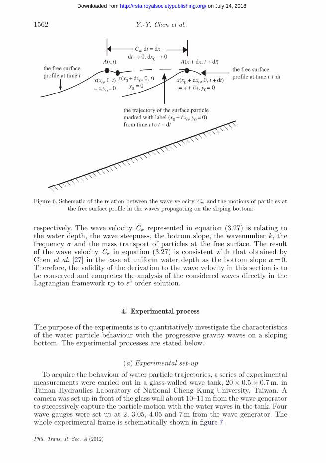
(e) The determination of the propagating velocity of the wave surface profileor the wave velocity Cw

Up to this point, all the properties for the considered waves could be directlyfound in the Lagrangian framework. The only unsolved property needing tobe determined is the wave velocity Cw since it is varying with the wavesurface position and still unknown. The wave velocity Cw of the consideredwaves can be obtained as outlined below as shown in figure 6. Consider asurface particle marked with label (x0, y0 = 0) that is located at a point Aof the free surface with the horizontal coordinate x(x0, y0 = 0, t) = x and thephase q = ∫x0 k(x ′

0)dx ′0 − st at time t. Along the propagating direction of the

free surface, when time t + dt, dt → 0, the point A with the wave velocityCw moves a horizontal distance Cwdt to a new position where an adjacentsurface particle marked with label (x0 + dx0, y = 0) travels from time t tot + dt to there just to meet it. So, the horizontal coordinate of the newposition of the point A at the free surface at time t + dt is x(x0 + dx0,y0 = 0, t + dt) = x + dx . From the statement above, two necessary equations fordetermining the wave velocity Cw can be written, where the phase q = constantand dt → 0, dx0 → 0, as follows:

q =∫ x0

k(x ′0)dx ′

0 − st =∫ x0+dx0

k(x ′0)dx ′

0 − s(t + dt) = constant, y0 = 0 (3.24)

and

Cwdt = dx = x(x0 + dx0, y0 = 0, t + dt) − x(x0, y0 = 0, t), (3.25)

where

x(x0, y0, t) = x0 +∞∑

m=1

∞∑n=0

3man[fm,n

(∫ x0

kdx ′0 − st, y0

)+ f ′

m,n(x0, y0, s0t)].

(3.26)





a = 1/10k'0,0H = 0.06p

0.8(a) (b) (c) (e) ( f ) (g)(d)

free surface0.4

0

–0.4

–0.8–8 –7 –6 –5 –4 –3 –2 –1 0

k'0,

0 y

k'0,0x

k'0,0x0 = –7.5

k'0,0y0 = –0.15

k'0,0y0 = 0

k'0,0y0 = –0.45

k'0,0y0 = –0.75

k'0,0y0 = –0.3

k'0,0y0 = –0.6

k'0,0x0 = –6

k'0,0y0 = –0.12

k'0,0y0 = –0.24k'0,0y0 = –0.36

k'0,0y0 = –0.48

k'0,0y0 = –0.6

k'0,0y0 = 0

(b)

0.2

0.4

0

–0.2

–0.4

–0.6

–0.8–7.9 –7.7 –7.5 –7.3 –7.1

k'0,

0 y

k'0,0x0 = –5

k'0,0y0 = 0

k'0,0y0 = –0.1

k'0,0y0 = –0.3

k'0,0y0 = –0.5

k'0,0y0 = –0.2

k'0,0y0 = –0.4

k'0,0x0 = –3

k'0,0y0 = 0

k'0,0y0 = –0.06

k'0,0y0 = –0.18k'0,0y0 = –0.12

k'0,0y0 = –0.24

k'0,0x0 = –4

k'0,0y0 = 0

k'0,0y0 = –0.08

k'0,0y0 = –0.24

k'0,0y0 = –0.4

k'0,0y0 = –0.16

k'0,0y0 = –0.32

k'0,0x0 = –2.8

k'0,0y0 = 0

k'0,0y0 = –0.056

k'0,0y0 = –0.168k'0,0y0 = –0.112

k'0,0y0 = –0.224

(d) 0.4

0.2

0

–0.2

–0.4

–0.6–5.4 –5.2 –5.0 –4.8 –4.6

k'0,

0y

( f )

k'0,0x

0.4

0.2

0

–0.2

–0.6

–0.4

–3.4 –3.2 –3.0 –2.8 –2.6

k'0,

0y

(g)

k'0,0x

0.4

0.2

0

–0.2

–0.6

–0.4

–3.2 –3.0 –2.8 –2.6 –2.4

(e) 0.4

0.2

0

–0.2

–0.4

–4.4 –4.2 –4.0 –3.8 –3.6–0.6

(c) 0.4

0.2

0

–0.2

–0.4

–0.6

–0.8–6.4 –6.2 –6.0 –5.8 –5.6


The solutions of equations (3.24) and (3.25) are easily to be obtained by usingequation (3.26), which are

dx0 = s

kdt and Cw = s

k+

∞∑m=1

∞∑n=0

3man[

s

k

f ′m,n

vx0+ f ′

m,n

vt

], y0 = 0,

vj fm,n

vxj0

= O(aj),

(3.27)





the free surfaceprofile at time t

Cw dt = dxdt Æ 0, dx0 Æ 0

the trajectory of the surface particlemarked with label (x0 + dx0, y0 = 0)from time t to t + dt

the free surfaceprofile at time t + dt

A(x + dx, t + dt)

x(x0, 0, t)

A(x,t)

= x,y0 = 0

x(x0 + dx0, 0, t) x(x0 + dx0, 0, t + dt)= x + dx, y0= 0y0 = 0

Figure 6. Schematic of the relation between the wave velocity Cw and the motions of particles atthe free surface profile in the waves propagating on the sloping bottom.

respectively. The wave velocity Cw represented in equation (3.27) is relating tothe water depth, the wave steepness, the bottom slope, the wavenumber k, thefrequency s and the mass transport of particles at the free surface. The resultof the wave velocity Cw in equation (3.27) is consistent with that obtained byChen et al. [27] in the case at uniform water depth as the bottom slope a = 0.Therefore, the validity of the derivation to the wave velocity in this section is tobe conserved and completes the analysis of the considered waves directly in theLagrangian framework up to 33 order solution.

4. Experimental process

The purpose of the experiments is to quantitatively investigate the characteristicsof the water particle behaviour with the progressive gravity waves on a slopingbottom. The experimental processes are stated below.

(a) Experimental set-up

To acquire the behaviour of water particle trajectories, a series of experimentalmeasurements were carried out in a glass-walled wave tank, 20 × 0.5 × 0.7 m, inTainan Hydraulics Laboratory of National Cheng Kung University, Taiwan. Acamera was set up in front of the glass wall about 10–11 m from the wave generatorto successively capture the particle motion with the water waves in the tank. Fourwave gauges were set up at 2, 3.05, 4.05 and 7 m from the wave generator. Thewhole experimental frame is schematically shown in figure 7.





20 m

10 m

d

7.55 m

0.7 m

2 m 1.05 m 1 m 2.95 m 2 m

wave generator shoot zone

camera

Figure 7. Experimental frame and instrument set-up.

(b) Experimental procedure

— Monochromatic free surface progressive gravity water waves weregenerated using a piston-type wave generator.

— Measurements of incident progressive wave elevations were made using aNijin capacity wave height meter.

— Water particles were simulated with spherical polystyrene beads (PS) offluorescent red colour with a diameter of about 0.1 cm. The density ofprimitive PS in a normal state is about 1.05 g cm−3 heavier than the water.When it is boiled its volume will swell until the density of PS approximatelyequals water density, 1.000 g cm−3.

— Images were captured by a Sony HDR-SR12 digital HD video camera,which has a 1920 × 1080 pixel resolution and 29.97 frames per secondmaximum framing rate.

— A transparent acrylic-plastic sheet (1 m × 45 cm × 2 mm), which wasplaced in the plane of the PS motion position, was calibrated at 1 mmintervals in 5 × 5 mm grids. Its function is a virtual grid in the picture.The trajectory of the PS motion in the water waves could be inferred fromthe PS motion image data and virtual grid.

(c) Experimental results

The particle motion experiments were conducted at a constant water depthd (0.367 m) and various wave periods T (0.80–2.35 s). The wave height H wasvaried over a range 0.0385–0.0672 m. All of the experimental wave conditionsare shown in table 1. k ′

0,0x0 is the dimensionless initial position of a PS particle.The measured orbital results are shown in figure 8. In figure 8, the two brighthorizontal lines are the SWL at both sides of the tank. As in the case of shallowwater depth, there is a clearly downward convex shape in the particle orbit,shown in figure 8a,b. In figure 8c, the PS particle orbit is similar to an ellipse; infigure 8d,e, the orbits are non-closed circles.

5. Results and discussion

(a) Verification of the theoretical solution

Verifications of the theoretical solution up to the third order are given below.(i) In order to verify the theoretical solutions presented above both

mathematically and physically, we first prove the asymptotic behaviour for thedeep-water limit, as d = d0 → ∞. In this zone, k = k0,0 = k ′

0,0, a = a0, D = D0 = 1,





(a) (b) (c)

(d) (e)

Figure 8. (a–e) The experimental particle trajectories at five wave conditions.

Table 1. Experimental conditions of particle orbit.

no. T (s) H (m) d (m) a k ′0,0x0

a 2.35 0.0385 0.376 1/10 2.3b 1.74 0.0397 0.376 1/10 3.2c 2.00 0.0672 0.376 1/10 4d 1.01 0.0628 0.376 1/10 7e 0.80 0.0440 0.376 1/10 9

S = k ′0,0x0 − st. Theoretical solutions in deep water can be easily shown to be

x = f1,0 + f ′2,0 + f3,0 = a0ek ′

0,0y0 sin S + a20k

′0,0e

2k ′0,0y0s0t

−[2a3

0k20,0e

3k ′0,0y0 − 1

2a3

0k′20,0e

k ′′0,0y0

]sin S ,

y = g1,0 + g3,0 = a0ek ′0,0y0 cos S + 1

2a2

0k′0,0e2k ′

0,0y0

+[a3

0k20,0e

3k ′0,0y0 − 1

2a3

0k′20,0e

k ′0,0y0

]cos S ,

f = f1,0 = −s0,0

k0a0ek ′

0,0y0 sin S ,

s20,0 = gk ′

0,0,

s2,0 = s0a20k

′20,0

(−e2k ′

0,0y0 + 12

)and s = s0,0 + s2,0,

⎫⎪⎪⎪⎪⎪⎪⎪⎪⎪⎪⎪⎪⎪⎪⎪⎪⎪⎪⎪⎪⎪⎪⎪⎪⎪⎬⎪⎪⎪⎪⎪⎪⎪⎪⎪⎪⎪⎪⎪⎪⎪⎪⎪⎪⎪⎪⎪⎪⎪⎪⎪⎭

(5.1)

which are the same as those given by Chen et al. [27] in deep water and hencethe theory is verified. Apparently, the water particle trajectory in deep water issymmetric and the present deep water solution does not encompass the bottomeffect. Constantin and co-workers [41–43] show the symmetry property holds evenfor waves of large amplitude in the presence of underlying vorticity.





(ii) Constant horizontal depth, viz. d = dc and a = 0. This case describes finiteamplitude waves over a constant depth. Since in this case

k0,0 = k0,0c; a = ac; S = k0,0cx0 − st,for the case of a = 0 the theoretical solution becomes

x = f1,0 + f2,0 + f ′2,0 + f3,0 = −ac

cosh k0,0c(y0 + dc)sinh k0,0cdc

sin S

− 38a2

c k0,0ccosh 2k0,0c(y0 + dc)

sinh4 k0,0cdcsin 2S + 1

4a2

c k0,0csin 2S

sinh2 k0,0cdc

+ 12a2

c k0,0ccosh 2k0,0c(y0 + dc)

sinh2 k0,0cdcs0,0t +

[−b3c

cosh 3k0,0c(y0 + dc)

sinh3 k0,0cdc

+ 16k0,0c(5B1,0,1cB2,0c − 2B1,0,1cC2,0c) cosh k0,0c(y0 + dc)

]sin 3S

−[12k0,0c(5B1,0,1cB2,0c + 4B1,0,1cC2,0c) cosh 3k0,0c(y0 + dc)

+ l3c cosh k0,0c(y0 + dc)

sinh3 k0,0cdc

]sin S ,

y = g1,0 + g2,0 + g3,0 = acsinh k0,0c(y0 + dc)

sinh k0,0cdccos S

+ 38a2

c k0,0csinh 2k0,0c(y0 + dc)

sinh4 k0,0cdcos 2S + 1

4a2

0k0,0csinh 2k0,0c(y0 + dc)

sinh2 k0,0cdc

+[

b3csinh 3k0,0c(y0 + dc)

sinh3 k0,0cdc− 1

2k0,0cB1,0,1cB2,0c sinh k0,0c(y0 + dc)

]cos 3S

+[12k0,0(3B1,0,1cB2,0c + 2B1,0,1cC2,0c) sinh 3k0,0c(y0 + d)

+ l3csinh k0,0c(y0 + dc)

sinh3 k0,0cdc+ k2,0cB1,0,1c(y0 + dc) cosh k0,0c(y0 + dc)

]cos S ,

f = f1,0 + f2,0 + f′2,0 + f3,0 = acs0,0

k0,0c

cosh k0,0c(y0 + dc)sinh k0,0cdc

sin S

+ 38a2

c s0,0cosh 2k0,0c(y0 + dc)

sinh4 k0,0cdcsin 2S − 1

2a2

c s0,01

sinh2 k0,0cdcsin 2S

− 14a2

c s20,0

1

sinh2 k0,0cdct + s0

k0,0cb3c

cosh 3k0,0c(y0 + dc)

sinh3 k0,0cdcsin 3S

+ 12

s0B1,0,1cB2,0c cosh 3k0,0c(y0 + dc) sin S − 12

s0B1,0,1c(3B2,0c − 2C2,0c)

× cosh k0,0c(y0 + dc) sin 3S , s20,0 = gk0,0c tanh k0,0cdc,

sw2c = 116

k20,0ca

2c s0(9 coth4 k0,0cdc − 10 coth2 k0,0cdc + 9)

and s2 = −12

s0Bc1,0,1k

20,0c cosh 2k0,0c(y0 + dc) + sw2c,

⎫⎪⎪⎪⎪⎪⎪⎪⎪⎪⎪⎪⎪⎪⎪⎪⎪⎪⎪⎪⎪⎪⎪⎪⎪⎪⎪⎪⎪⎪⎪⎪⎪⎪⎪⎪⎪⎪⎪⎪⎪⎪⎪⎪⎪⎪⎪⎪⎪⎪⎪⎪⎪⎪⎪⎪⎪⎪⎪⎪⎪⎪⎪⎪⎪⎪⎪⎪⎪⎪⎪⎪⎪⎬⎪⎪⎪⎪⎪⎪⎪⎪⎪⎪⎪⎪⎪⎪⎪⎪⎪⎪⎪⎪⎪⎪⎪⎪⎪⎪⎪⎪⎪⎪⎪⎪⎪⎪⎪⎪⎪⎪⎪⎪⎪⎪⎪⎪⎪⎪⎪⎪⎪⎪⎪⎪⎪⎪⎪⎪⎪⎪⎪⎪⎪⎪⎪⎪⎪⎪⎪⎪⎪⎪⎪⎪⎭(5.2)





0.8(a)

(b)

e3a0

e3a0e2a0e1a1

e2a0

e1a10.4

0

–0.4

–0.8

0.20

0.10

0

–0.10

–0.20

–0.30–1.5 –1.0 –0.5 0

–5.0 –4.0 –3.0 –2.0 –1.0 0

a = 1/10k'0,0H = 0.1p

a = 1/5k'0,0H0 = 0.02p

k'0,

0h

k'0,0x

k'0,

0h

Figure 9. (a, b) Successive wave profiles prior to breaking plotted by linear (up to the order of 31a1)and nonlinear solutions (up to the order of 32a0 and up to the order of 33a0) under varying waveconditions and bottom slopes. (Solid line, third-order solution; dotted line, second-order solution;dashed line, linear solution.)

where the coefficients b3c, l3c, B2,0c, C2,0c and Bc1,0,1 are

b3c = 164

a3c k

20,0c(9 coth4 k0,0cdc − 22 coth2 k0,0cdc + 13),

l3c = − 116

k30,0ca

2c (9 coth4 k0,0cdc − 10 coth2 k0,0cdc + 9) sinh2 k0,0cdc,

B2,0c = 38B2

1,0,1ck0,0c1

sinh2 k0,0cdc,

C2,0c = 14B2

1,0,1ck0,0c

and Bc1,0,1 = ac

sinh k0,0cdc.

The present theory is reduced to a nonlinear wave over water of constant depth,as was previously obtained by Chen et al. [27]. Thus, the present theory is verified.





0.8(a) (b)

–5.2 –4.7 –3.7 –3.2–4.2

0.4

0

–0.4

–0.8–8 –7 –6 –5 –4 –3 –2 –1 0

k'0,

0 y

k'0,0x k'0,0x

a = 1/10k'0,0H = 0.1p k'0,0x0 = –4.2

Figure 10. (a, b) The particle trajectories near the wave-breaking point for a spilling wave. (Solidline, up to 33a0 order; dashed line, up to 32a0 order.)

0.20.4

0.2

0

–0.2

–0.4–1.8 –1.6 –1.4 –1.2 –1.0 –0.8

(b)

0.1

0

–0.1

–0.2

–0.3–1.75 –1.65 –1.55 –1.45 –1.35

(a)

k'0,

0 y

k'0,0x k'0,0x

a = 1/10k'0,0H = 0.02p k'0,0x0 = –1.55

Figure 11. (a, b) The particle trajectories near the wave-breaking point for a plunging wave. (Solidline, up to 33a0 order; dashed line, up to 32a0 order.)

(b) Wave transformations

As the height of a wave reaches its upper limit, the crest is fully developedas a summit that can be calculated as the spatial surface profile by a systemof Lagrangian coordinates. In this approach, the new displacement componentsof water particles x and y to the third-order approximation have been obtainedas follows:

x(x0, y0, t) = x0 + 31a0f1,0 + 31a1f1,1 + 32a0(f2,0 + f ′2,0) + 33a0f3,0 (5.3)

andy(x0, y0, t) = y0 + 31a0g1,0 + 31a1g1,1 + 32a0g2,0 + 33a0g3,0. (5.4)

The surface wave profiles near the wave breaking point can be evaluated and theresults are illustrated in figure 9. The linear (up to the order 31a1) and nonlinearsolutions (up to the orders 32a0 and 33a0) are implemented for comparison. Thisfigure shows the surface wave profiles prior to breaking on different wave steepnessand wave phase for bottom slopes of a = 1/5 and 1/10, respectively, based on thewave breaking criterion of u/Cw = 1. It is found that the third-order theory isconsistent with the classification of wave breakers proposed by Galvin [44]. Thisconfirms that the breaker type depends on the bottom slopes. In general, thethird-order wave profiles are higher than the second-order and linear solutions





0.10(a)

(c) (d)

(b)

0.05

–0.05

–0.10–2.45 –2.40 –2.35 –2.30 –2.25 –2.20 –2.15

0

0.15

0.10

0.05

0

–0.05

–0.10

–0.15–3.4 –3.3 –3.2 –3.1 –3.0

0.15

0.10

0.05

0

–0.05

–0.10

–0.15–4.2 –4.1 –4.0 –3.9 –3.8

0.4

0.2

0

–0.2

–0.4–7.4 –7.2 –7.0 –6.8 –6.6

0.4(e)

0.2

0

–0.2

–0.4–9.4 –9.2 –9.0 –8.8 –8.6

k'0,

0 y

k'0,

0 y

k'0,

0 y

k'0,0x

k'0,0x k'0,0x

k'0,0x0 = –2.3

k'0,0y0 = 0

k'0,0x0 = –3.2

k'0,0y0 = 0

k'0,0x0 = –4

k'0,0y0 = 0

k'0,0x0 = –7

k'0,0y0 = 0

k'0,0x0 = –9

k'0,0y0 = 0

Figure 12. (a–e) Comparisons between the orbits of water particles obtained by the third-ordersolution, second-order solution and those from the experimental measurements of the PS motions onsloping bottom (circle, experiment; solid line, the third-order solution; dashed line, the second-ordersolution). (The wave conditions are listed in table 1.)





for any wave steepness and bottom slope. Moreover, the breaking point predictedby the third-order solution occurs earlier than that by the second-order andlinear solutions.

(c) Particle orbits

The new Lagrangian solution for water particle displacement developed in thisstudy can be employed to demonstrate the validity for water particle motion.The parametric functions for the water particle at any position in Lagrangiancoordinates (x , y) are given in equations (5.3) and (5.4). Figures 10 and 11 showthe variation of particle trajectories under a spilling and plunging breaker. Owingto the second-order mass transport velocity which decreases exponentially withthe water depth, the particles do not move in a closed orbital motion and eachparticle advances a larger horizontal movement at the free surface. Near thebottom, the trajectory becomes more like an ellipse since the vertical excursion ofthe particle is less than its horizontal excursion, in contrast with the trajectoriesnear the mean water level. In the same deep water steepness, the second-orderorbital motion is smaller than the third-order orbital motion. Figure 12 showsgood agreement between the experimental data and the third-order asymptoticsolution of the particle trajectories at the free surface.

6. Conclusions

This paper provides a new third-order Lagrangian asymptotic solution for surfacewaves propagating over a uniform sloping beach. The solution, developed inexplicit form, includes parametric functions for water particle motion and thewave velocity in Lagrangian description. These explicit expressions enable thedescription of wave shoaling in the direction of wave propagation from deep toshallow water. The solution also provides information for the process of successivedeformation of a wave profile and water particle trajectory. The solution to thenonlinear boundary-value problem is presented after including a mean returncurrent which is needed to maintain zero mass flux in a bounded domain. Also,the Lagrangian mean level differing from the Eulerian mean level is explicitlyobtained via a new third-order solution. Furthermore, to check the validity of thenonlinear analytical solution, it is shown analytically that, in the limit of deepwater or constant depth, the nonlinear solution reduces to the known Lagrangianthird-order solution of progressive waves. A series of experiments measuringthe Lagrangian properties of nonlinear water waves propagating over a slopingbottom were conducted in a wave tank. Good agreement has been obtained oncomparing the measured trajectories with the theoretical trajectories predictedby the proposed third-order Lagrangian solution.

Dr K. S. Hwang is appreciated for his laboratory assistance. The work was supported by theResearch Grant Council of the National Science Center, Taiwan, through project no. NSC99-2923-E-110-001-MY3 and no. NSC99-2221-E-110 -087-MY3.

References

1 Segur, H. 2007 Waves in shallow water, with emphasis on the tsunami of 2004. In Tsunami andnonlinear waves, pp. 3–29. Berlin, Germany: Springer.





2 Constantin, A. & Johnson, R. S. 2008 Propagation of very long water waves, withvorticity, over variable depth, with applications to tsunamis. Fluid Dyn. Res. 40, 175–211.(doi:10.1016/j.fluiddyn.2007.06.004)

3 Biesel, F. 1952 Study of wave propagation in water of gradually varying depth. Gravity waves.Circular 521, pp. 243–253, US National Bureau of Standards.

4 Chen, Y.-Y. & Tang, L. W. 1992 Progressive surface waves on gentle sloping bottom. InProc. 14th Ocean Engineering Conf. in Taiwan, pp. 1–22. Taiwan: Taiwan Society of OceanEngineering. [In Chinese.]

5 Carrier, G. F. & Greenspan, H. P. 1958 Water waves of finite amplitude on a sloping beach.J. Fluid Mech. 4, 97–109. (doi:10.1017/S0022112058000331)

6 Chu, V. H. & Mei, C. C. 1970 On slowly-varying Stokes waves. J. Fluid Mech. 41, 873–887.(doi:10.1017/S0022112070000988)

7 Liu, P. L. F. & Dingemans, M. W. 1989 Derivation of the third-order evolution equationsfor weakly nonlinear water waves propagating over uneven bottoms. Wave Motion 11, 41–64.(doi:10.1016/0165-2125(89)90012-7)

8 Chen, Y.-Y., Hsu, H.-C., Chen, G.-Y. & Hwung, H.-H. 2006 Theoretical analysis of surfacewaves shoaling and breaking on a sloping bottom. II. Nonlinear waves. Wave Motion 43, 339–356. (doi:10.1016/j.wavemoti.2006.01.002)

9 Chen, Y.-Y. & Hsu, H.-C. 2009 A third-order asymptotic solution of nonlinear standing waterwaves in Lagrangian coordinates. Chin. Phys. B 18, 861–871. (doi:10.1088/1674-1056/18/3/004)

10 Naciri, M. & Mei, C. C. 1993 Evolution of short gravity waves on long gravity waves. Phys.Fluids A 5, 1869–1878. (doi:10.1063/1.858812)

11 Ng, C. O. 2004 Mass transport in a layer of power-law fluid forced by periodic surface pressure.Wave Motion 39, 241–259. (doi:10.1016/j.wavemoti.2003.10.002)

12 Ng, C. O. 2004 Mass transport and set-ups due to partial standing surface waves in a two layerviscous system. J. Fluid Mech. 520, 297–325. (doi:10.1017/S0022112004001624)

13 Ng, C. O. 2004 Mass transport in gravity waves revisited. J. Geophys. Res. Oceans 109, C04012.(doi:10.1029/2003JC002121)

14 Chen, Y.-Y., Hwung, H.-H. & Hsu, H.-C. 2005 Theoretical analysis of surface waves propagationon sloping bottoms. I. Wave Motion 42, 335–351. (doi:10.1016/j.wavemoti.2005.04.004)

15 Zhang, X. & Ng, C.-O. 2006 On the oscillatory and mean motions due to waves in thinviscoelastic layer. Wave Motion 43, 387–405. (doi:10.1016/j.wavemoti.2006.02.003)

16 Buldakov, E. V., Taylor, P. H. & Taylor, R. E. 2006 New asymptotic description ofnonlinear water waves in Lagrangian coordinates. J. Fluid Mech. 562, 431–444. (doi:10.1017/S0022112006001443)

17 Ng, C. O. & Zhang, X. Y. 2007 Mass transport in water waves over a thin layer of softviscoelastic mud. J. Fluid Mech. 573, 105–130. (doi:10.1017/S0022112006003508)

18 Gerstner, F. J. 1802 Theorie de wellen. Abh. d. K. bohm. Ges. Wiss. 32, 412–440. [Reprintedin Ann. Physik.]

19 Miche, A. 1944 Mouvements ondulatoires de la mer en profondeur constante ou décroissante.Annal. Ponts Chaussees 114, 25–78, 131–164, 270–292, 369–406.

20 Pierson, W. J. 1962 Perturbation analysis of the Navier-Stokes equations in Lagrangian formwith selected linear solution. J. Geophys. Res. 67, 3151–3160. (doi:10.1029/JZ067i008p03151)

21 Constantin, A. 2006 The trajectories of particles in Stokes waves. Invent. Math. 166, 523–535.(doi:10.1007/s00222-006-0002-5)

22 Constantin, A. & Escher, J. 2007 Particle trajectories in solitary water waves. Bull. Am. Math.Soc. 44, 423–431. (doi:10.1090/S0273-0979-07-01159-7)

23 Constantin, A. & Strauss, W. 2010 Pressure beneath a Stokes wave. Commun. Pure Appl.Math. 53, 533–557. (doi:10.1002/cpa.20299)

24 Constantin, A. & Escher, J. 2011 Analyticity of periodic traveling freesurface water waves withvorticity. Ann. Math. 173, 559–568. (doi:10.4007/annals.2011.173.1.12)

25 Ehrnström, M. & Wahlen, E. 2008 On the fluid motion in standing waves. J. Nonlinear Math.Phys. 15, 74–86. (doi:10.2991/jnmp.2008.15.s2.6)

26 Hsu, H.-C., Chen, Y.-Y. & Wang, C.-F. 2010 Perturbation analysis of the short-crestedwaves in Lagrangian coordinates. Nonlinear Anal. Ser. B: Real World Appl. 11, 1522–1536.(doi:10.1016/j.nonrwa.2009.03.014)



http://dx.doi.org/doi:10.1016/j.fluiddyn.2007.06.004

http://dx.doi.org/doi:10.1017/S0022112058000331


http://dx.doi.org/doi:10.1016/0165-2125(89)90012-7

http://dx.doi.org/doi:10.1016/j.wavemoti.2006.01.002

http://dx.doi.org/doi:10.1088/1674-1056/18/3/004

http://dx.doi.org/doi:10.1063/1.858812



http://dx.doi.org/doi:10.1029/2003JC002121






http://dx.doi.org/doi:10.1029/JZ067i008p03151

http://dx.doi.org/doi:10.1007/s00222-006-0002-5

http://dx.doi.org/doi:10.1090/S0273-0979-07-01159-7

http://dx.doi.org/doi:10.1002/cpa.20299

http://dx.doi.org/doi:10.4007/annals.2011.173.1.12

http://dx.doi.org/doi:10.2991/jnmp.2008.15.s2.6

http://dx.doi.org/doi:10.1016/j.nonrwa.2009.03.014



27 Chen, Y.-Y., Hsu, H.-C. & Chen, G.-Y. 2010 Lagrangian experiment and solution forirrotational finite-amplitude progressive gravity waves at uniform depth. Fluid Dyn. Res. 42,045511. (doi:10.1088/0169-5983/42/4/045511)

28 Sanderson, B. 1985 A Lagrangian solution for internal waves. J. Fluid Mech. 152, 191–202.(doi:10.1017/S0022112085000647)

29 Constantin, A. 2001 Edge waves along a sloping beach. J. Phys. A 34, 9723–9731.(doi:10.1088/0305-4470/34/45/311)

30 Chen, Y.-Y. & Huang, C.-Y. 2000 Surface-waves propagation on a gentle bottom in Lagrangianform. In Proc. 22nd Conf. on Ocean Engineering in Taiwan, pp. 79–88. Taiwan: Taiwan Societyof Ocean Engineering. [In Chinese.]

31 Kapinski, J. 2006 On modeling of long waves in the Lagrangian and Eulerian descriptions.Coastal Eng. 53, 759–765. (doi:10.1016/j.coastaleng.2006.03.009)

32 Chen, Y.-Y. 1994 Perturbation analysis of the irrotational progressive gravity waves in fluidof any uniform depth in Lagrangian form. In Proc. 16th Ocean Engineering Conf. in Taiwan,pp. A1–A29. Taiwan: Taiwan Society of Ocean Engineering. [In Chinese.]

33 Lamb, H. 1932 Hydrodynamics, 6th edn. Cambridge, UK: Cambridge University Press.34 Yakubovich, E. I. & Zenkovich, D. A. 2001 Matrix approach to Lagrangian fluid dynamics.

J. Fluid Mech. 443, 167–196. (doi:10.1017/S0022112001005195)35 Chen, Y.-Y. 2003 Nonlinear analysis for surface waves propagation on non-steep sloping bottom.

I. Systematical perturbation expansion model. In Proc. 25th Conf. on Ocean Engineering inTaiwan, pp. 39–48. Taiwan: Taiwan Society of Ocean Engineering. [In Chinese.]

36 Chen, Y.-Y. 2003 Nonlinear analysis for surface waves propagation on non-steep sloping bottom.II. Analytical solution up to order and verification. In Proc. 25th Conf. on Ocean Engineeringin Taiwan, pp. 49–58. Taiwan: Taiwan Society of Ocean Engineering. [In Chinese.]

37 Longuet-Higgins, M. S. 1953 Mass transport in water waves. Phil. Trans. R. Soc. Lond. A 245,535–581. (doi:10.1098/rsta.1953.0006)

38 Longuet-Higgins, M. S. 1986 Eulerian and Lagrangian aspects of surface waves. J. Fluid Mech.173, 683–707. (doi:10.1017/S0022112086001325)

39 Longuet-Higgins, M. S. & Stewart, R. W. 1964 Radiation stress in water waves—a physicaldiscussion with applications. Deep Sea Res. 11, 529–562. (doi:10.1016/0011-7471(64)90001-4)

40 Constantin, A. & Varvaruca, E. 2011 Steady periodic water waves with constant vorticity:regularity and local bifurcation. Arch. Ration. Mech. Anal. 119, 33–67. (doi:10.1007/s00205-010-0314-x)

41 Constantin, A. & Escher, J. 2004 Symmetry of steady periodic surface water waves withvorticity. J. Fluid Mech. 498, 171–181. (doi:10.1017/S0022112003006773)

42 Constantin, A. & Escher, J. 2004 Symmetry of steady deep-water waves with vorticity. Eur. J.Appl. Math. 15, 755–768. (doi:10.1017/S0956792504005777)

43 Constantin, A., Ehrnstrom, M. & Wahlen, E. 2007 Symmetry of steady periodic gravity waterwaves with vorticity. Duke Math. J. 140, 591–603. (doi:10.1215/S0012-7094-07-14034-1)

44 Galvin, C. J. 1968 Breaker type classification on three laboratory beaches. J. Geophys. Res. 73,3651–3659. (doi:10.1029/JB073i012p03651)






http://dx.doi.org/doi:10.1016/j.coastaleng.2006.03.009


http://dx.doi.org/doi:10.1098/rsta.1953.0006


http://dx.doi.org/doi:10.1016/0011-7471(64)90001-4

http://dx.doi.org/doi:10.1007/s00205-010-0314-x

http://dx.doi.org/doi:10.1007/s00205-010-0314-x



http://dx.doi.org/doi:10.1215/S0012-7094-07-14034-1

http://dx.doi.org/doi:10.1029/JB073i012p03651


Theoretical and experimental study of particle...

Documents

Transcript of Theoretical and experimental study of particle...