THEORETICAL ANALYSIS OF SMALL CRACK GROWTH IN FIBER ...
94
THEORETICAL ANALYSIS OF SMALL CRACK GROWTH IN FIBER-REINFORCED CERAMIC COMPOSITE MATERIALS by FORREST T PATTERSON B.S., Mechanical Engineering University of California, Berkeley (1989) M.S., Mechanical Engineering Stanford University (1990) Submitted to the Department of Mechanical Engineering in Partial Fulfillment of the Requirements for the Degree of DOCTOR OF PHILOSOPHY IN MECHANICAL ENGINEERING at the MASSACHUSETTS INSTITUTE OF TECHNOLOGY May 1994 © Massachusetts Institute of Technology, 1994. All rights reserved. Signature of Authol Department of Mechanical Engineering S./May, 1994 Certified by / Professor Michael P. Cleary Thesis Supervisor Accepted by - Professor Ain A. Sonin Chairman, Mechanical Engineering Department Committee Eng.• ii MA SA(, - - t Ir•t "-C ~·s ~ LAE
Transcript of THEORETICAL ANALYSIS OF SMALL CRACK GROWTH IN FIBER ...

THEORETICAL ANALYSIS OF SMALL CRACK GROWTHIN FIBER-REINFORCED CERAMIC COMPOSITE MATERIALS
by
FORREST T PATTERSON
B.S., Mechanical EngineeringUniversity of California, Berkeley (1989)
M.S., Mechanical EngineeringStanford University (1990)
Submitted to the Department ofMechanical Engineering
in Partial Fulfillment of the Requirementsfor the Degree of
DOCTOR OF PHILOSOPHYIN MECHANICAL ENGINEERING
at theMASSACHUSETTS INSTITUTE OF TECHNOLOGY
May 1994
© Massachusetts Institute of Technology, 1994. All rights reserved.
Signature of AutholDepartment of Mechanical Engineering
S./May, 1994
Certified by / Professor Michael P. ClearyThesis Supervisor
Accepted by -Professor Ain A. Sonin
Chairman, Mechanical Engineering Department Committee
Eng.•ii MA SA(, - - t Ir•t "-C
~·s ~ LAE

THEORETICAL ANALYSIS OF SMALL CRACK GROWTH IN FIBER-REINFORCED CERAMIC COMPOSITE MATERIALS
by
FORREST T PATTIERSON
Submitted to the Department of Mechanical Engineeringin May, 1994 in partial fulfillment of the
requirements for the Degree of Doctor of Philosophy
Abstract
This research program investigates matrix crack initiation and subsequentpropagation in fiber-reinforced ceramic materials for use in high-temperature structuralapplications.
Though it presents a formidable manufacturing challenge, the inclusion ofceramic fibers promises to increase fracture toughness and improve failure modesthrough crack deflection, fracture bridging, and frictional interface slip. Experimentalobservations show that ceramic composites initially fail at several points in the matrixand along the interfaces. These small cracks and inherent processing flaws propagate andcoalesce, forming large cracks that lead to component failure. Therefore, anunderstanding of small crack growth is necessary for the design of composite systemswhich delay critical crack formation and which fail in a desirable manner.
The Surface Integral and Boundary Element Hybrid (SIBEH) method, supportedby experimental observations, has been developed to model crack growth in brittle com-posite systems. The surface integral method models fractures as a piece-wise continuousdistribution of displacement discontinuities. When combined with traditional boundaryelement methods, the technique provides an efficient tool for modeling three-dimensionalcrack growth.
This approach has been used to model matrix crack initiation in a lithiumalumino-silicate (LAS) glass-ceramic that has been reinforced with continuous siliconcarbide fibers. By modeling the effects of crack pinning and bridging, interfacialdebonding, and frictional interface slip, this investigation aims to determine the stressesrequired for matrix crack initiation and the material parameters which promote 'graceful'failure modes. These results have been compared to existing analytical solutions forsmall crack growth. Results of this investigation are expected to be useful in developingguidelines for the manufacture and design of ceramic materials for high-temperaturestructural applications.
Thesis Supervisor: Michael P. ClearyTitle: Adjunct Professor of Mechanical Engineering

Acknowledgements
I am indebted to the Air Force Office of Scientific Research for funding myeducation and for sponsoring this research project through the Laboratory GraduateFellow Program and Grant No. AFOSR-89-005. Dr. Alan Burkhard's personalmentorship and the management of Professort W.D. Peele are greatly appreciated.
Special thanks are due my family of friends and relations who have providedencouragement, guidance, and support throughout my tenure at M.I.T. Successfulcompletion of my thesis research and doctoral degree would not have been possiblewithout their help. Professor Cleary has provided direction and support for my researchand teaching interests while allowing me freedom to explore and learn. For helping menavigate the sea of bureaucracy, I thank the staff of the department, including LeslieRegan, Joan Kravit, Susan Melillo, Lucy Piazza, Marie Pommet, Maureen DeCourcey,and John O'Brien.
For their help preparing for qualifying exams, I am indebted to Ashok Patel, DaleWatring, and John Wlassich. I also am grateful for the guidance and insightfulsuggestions of Professors Bill Keat, Michael Larson, D.M. Parks, J.J. Connor, and J.W.Hutchinson. Finally, I would like to thank the members of R.E.L. - most notably TimQuinn - for years of support and friendship. This thesis would not have been possiblewithout their daily support and laughter.
In spite of the distance involved, I have benefited from the love and friendship of myimmediate family, including my sister, Ketti, my grandparents, and my fiancee, Kelly.This thesis is dedicated to my parents, Chuck and Sandie, for inspiring me - by example -to greater personal and professional heights. For this love and support I am eternallygrateful.

Table of Contents
Acknowledgements .................................................................................................. 3Table of Contents ............................................................................................................ 4List of Figures ................................................................................................................. 6List of Tables .......................................................................................................... 7Chapter 1 Introduction ................................................................................................... 8
1.1 Ceramics as Structural Materials ............................................................ 81.2 Failure of Fiber-Reinforced Ceramics .................... ......... 11
1.2.1 Damage Development................................................................. 111.2.2 Failure Modes ................................................................................. 121.2.3 Large Crack Models................................................................... 141.2.4 Small Crack Models..................... .. ...... ................. 15
1.4 Research Scope .................................................................................................. 181.4.1 Silicon Carbide/ Lithium Alumino-Silicate System ........................... 201.4.2 General Assumptions ....................................................................... 201.4.3 Model Development and Results Presentation ................................... 21
Chapter 2 The Surface Integral Method .......................................................................... 232.1 Surface Integral Fundamentals........................................... 232.2 Discrete Formulation................................................... 242.3 Current Implementation ..................................................................................... 282.4 Fracture Model Results ...................................................... 32
2.5 Numerical Issues ................................................................................................ 34
Chapter 3 The Surface Integral and Boundary Element Hybrid (SIBEH) Method ....... 373.1 SIBEH Method Fundamentals ..................................... ..... ............. 37
3.1.1 Elastostatic Boundary Element Model................................................... 383.1.2 Hybrid Formulation.................................................................... 403.1.3 Multiple Region Models ........................................................................ 43
3.2 Current Implementation ..................................................................................... 443.2.1 Singular Integration Scheme ............................................................... 453.2.2 Boundary Conditions ............................................................................. 46
3.3 Bimaterial Interface Models............................................................................. 493.3.1 Interfacial Slip and Separation ........................................ ........ 513.3.2 Experimental Verification ...................... ........... 52

3.4 Numerical Issues ................................................................................................ 553.4.1 Solution Accuracy ............................................... 553.4.2 Improved Iterative Scheme ................................................................ 563.4.3 Computational Efficiency ...................................... ............. 58
Chapter 4 Small Matrix Crack Growth in Ceramic Composite Materials .................. 594.1 Small Matrix Crack Models ................................ 59
4.1.1 Matrix Crack Initiation........................................................................... 614.2 Fracture Parameter Results .................................................................. 65
4.2.1 Matrix Cracking Stress................................................................. 654.2.2 Fiber Stresses ..................................................... 65
4.3 Discussion of Results ................................................................................... 66
Chapter 5 Conclusions and Recommendations .............................................................. 695.1 Conclusions ................................................................................................. 695.2 Recommendations for Further Work ........................................ ......... 70
References ..................................................................... 72Appendix A Fundamental SIBEH Relations ................................................................ 77
A. 1 Fundamental Solutions - Surface Integral Method ........................................ 77A.1.1 Kelvin's Point-Force Solution ............................................................ 78A.1.2 Rongved's Point-Force Solution................................. .......... 78A.1.3 Displacement Discontinuity Solutions ....................................... 81
A.2 Fundamental Solutions - Boundary Element Method .................................... 83
A.3 Element Mapping Functions .......................................................................... 85
A.4 Element Shape Functions .......................................................................... 86
Appendix B Singular Integration Schemes .................................................................. 88
B.1 Singular Integration - Surface Integral Method ............................................. 88
B.2 Singular Integration - Boundary Element Method ......................................... 91

List of Figures
Figure 1.1 Dominant Toughening Mechanisms for Ceramic Materials ........................ 10Figure 1.2 Failure M ode M ap ........................................................................................ 13Figure 1.3 Small Matrix Crack Toughening Mechanisms ............................................. 16Figure 1.4 Toughened Ceramic Composite Load-Deflection Behavior ..................... 17
Figure 1.5 Matrix Cracking Stress Estimates for Small Fractures............................... 19Figure 2.1 Tensile and shear displacement discontinuity representation..................... 25
Figure 2.2 Nine-Noded Element Geometry ....................................... .......... 29
Figure 2.3 Summary of Element Shape Functions ..................................................... 31
Figure 2.4 Penny-Shaped Crack Subject to Internal Pressure .................................... 32
Figure 2.5 Elliptical Crack Subject to Internal Pressure ................................................ 33
Figure 2.6 Collinear Penny-Shaped Cracks Subject to Internal Pressure ................... 35
Figure 2.7 Stress-Intensity Factors for Collinear Penny-Shaped Cracks ....................... 35
Figure 2.8 Calculated Crack Opening Displacements for Penny-Shaped Interface
Flaws Subject to Internal Pressure ............................................................................... 36
Figure 3.1 Superposition of Surface Integral and Boundary Element Models .............. 41
Figure 3.2 Treatment of Dirichlet Corners.................................................................. 48
Figure 3.3 1/6 Symmetric Model of a Circular Crack in a Tensile Rod ........................ 50
Figure 3.4 Symmetric Model Error Estimates ..................................... ........ 50
Figure 3.5 Interface Slip Experiment ................................................................. 54
Figure 3.6 Experimental and Computational Interface Slip .......................................... 54
Figure 3.7 1/4 Symmetric Model of Interface Slip Experiment ................................. 55
Figure 4.1 Matrix Crack Initiation Configuration........................ ............. 60
Figure 4.2 Small Matrix Crack Configuration and Model Cell .................................. 62
Figure 4.3 Matrix Crack Initiation Model ................................................................... 63
Figure 4.4 Matrix Crack Configurations .................................... ........... 64Figure 4.5 Matrix Cracking Stress for Small Cracks ....................................... 66
Figure 4.6 Fiber Stress Contour Plots ................................................ 67
Figure 4.7 Peak Axial Fiber Stress for Proximal Fibers ............................................. 68
Figure A. 1 Concentrated Force Acting in Bimaterial Domain ................................... 79
Figure B.1 Local Coordinate Frame used for Singular Integration Scheme ............... 92

List of Tables
Table 2.1 Stress-Intensity Factors for Elliptical Crack ..................... 33Table 4.1 SiC/LAS Composite Material Properties ........................................ 61Table 4.2 Effective Toughness for Small Crack Propagation ........................................ 65

Chapter 1
Introduction
This investigation provides a fully three-dimensional analysis of small matrix
crack growth in brittle materials reinforced with continuous brittle fibers for use in high-
temperature structural applications. The project focuses on the influence of the fiber-
matrix interface on small matrix crack growth and on fiber failure and is intended to
supplement existing models by assessing the three-dimensional and bimaterial effects.
Although the approach developed is general, a particular composite system consisting of
lithium alumino-silicate (LAS) reinforced by silicon carbide fibers has been modeled to
facilitate comparison with experimental data and existing models. A modified analytical
expression is suggested for crack initiation and subsequent propagation.
1.1 Ceramics as Structural Materials
Ceramics are attractive structural materials because they offer high specific
strengths, excellent thermo-mechanical properties, chemical and environmental stability,
and low raw material costs [1]. For high-temperature applications, such as internal
combustion engines for automotive and aeronautical propulsion, the use of ceramics
offers great gains in efficiency because of their insulating properties and low thermal
expansion coefficients. In many proposed applications (e.g. aerospace propulsion
systems and alternate-cycle nuclear reactors), ceramics are the only possible material
choice due to extreme operating temperature requirements. In spite of these demands,

Chapter 1: Introduction
ceramic materials have found limited use in critical structural applications due to their
inherent brittle failure modes and notch sensitivity.
In the spirit of Griffith's brittle fracture investigations, research efforts aimed at
improving the reliability of structural ceramics have shifted in focus from flaw control
(i.e. minimizing the processing flaw size and density) to damage tolerance (i.e. improving
the material's resistance to existing flaws). The recognition of resistance curve behavior
in zirconia and the development of high-temperature reinforcing fibers sparked this shift
and has renewed interest in structural ceramics designed for toughened fracture behavior.
Subsequent experimental investigations and theoretical models have identified the
primary toughening mechanisms and quantified many of their effects [2].
These dominant toughening mechanisms are depicted in Figure 1.1 and include
transformation toughening, microcracking, and reinforcement by ductile or brittle
inclusions. The first two are process-zone mechanisms which contribute stress-induced,
volumetric dilation or softening (respectively) in the region of the crack tip and act to
shield the flaw from the imposed global stress state. These mechanisms contribute
modest gains in overall material toughness [2,3].
Additional gains in toughness can be achieved through bridging mechanisms,
which transfer a portion of the applied load to intact inclusions spanning the fracture
opening. This load 'shedding' acts to reduce the stress concentrations at the crack tip and
is accomplished through shear stresses acting across bonded or frictionally constrained
fiber/matrix interfaces. Ductile bridging of the fracture by bonded metallic particles can
enhance toughness significantly but is limited to lower temperature ranges by the melting
point and chemical reactivity of the inclusion [3]. Whisker or particle reinforcement by
brittle inclusions also results in improvements in material toughness (roughly 200-300%)
and offers higher operating temperature ranges [2].

Chapter 1: Introduction
'IL\
(e)
Figure 1.1 Dominant Toughening Mechanisms for Ceramic Materials; Dominanttoughening mechanisms for brittle ceramic materials include (a) transformation toughen-ing, (b) microcracking, (c) ductile reinforcement, (d) brittle whisker reinforcement, and(e) brittle fiber reinforcement.
The most significant increases in toughness can approach two orders of magnitude
and are realized through continuous fiber reinforcement. Although it presents formidable
manufacturing challenges, the incorporation of brittle fibers also offers material designers
opportunities for damage tolerant behavior and more 'graceful' failure modes. In addition
to the stress relief described above, local nonlinear effects such as debonding and fric-
tional slip along fiber/matrix interfaces can contribute to the overall material toughness
[1,2]. The strong influence of interfacial properties on these toughening mechanisms has

Chapter 1: Introduction
been demonstrated and suggests tremendous opportunities for designing ceramic
materials. However, tailoring of the interface for toughened behavior remains the single
greatest challenge for successful development of ceramic composites.
1.2 Failure of Fiber-Reinforced Ceramics
1.2.1 Damage Development
While little toughening occurs during the initial stages of damage development,
this process has a significant impact on the final failure mode and on the toughening
mechanisms available. Experimental observations show that 'large' matrix cracks (i.e.
fractures that span many fibers) initiate from manufacturing flaws in the matrix that are
typically on the order of the fiber spacing [4,5]. These small cracks propagate under
applied loads and coalesce, forming large fractures which eventually lead to component
failure [6,7].
Theoretical investigations of fracture growth in fiber-reinforced ceramics in which
the fiber and matrix are firmly bonded have shown that the stresses imposed on the fiber
by the crack tip are magnified significantly during small crack growth [8-10]. These
local stresses pose a risk to the integrity of the fibers and therefore to the toughened
failure modes which rely on them. To isolate the fibers from this stress concentration and
avoid early fiber failure, the interface must be sufficiently weak. Unfortunately, this
isolation also reduces the effectiveness of toughening and crack pinning mechanisms [7].
For these reasons, an understanding of the behavior of small crack growth in
ceramic materials reinforced with frictionally-constrained fibers is required to balance
these competing effects and to properly tailor the interface for toughened behavior. The
results of this investigation are expected to provide structural engineers with the
necessary tools to evaluate the integrity of ceramic composite components and to provide

Chapter 1: Introduction
material scientists with an understanding of how interfacial effects affect the overall
composite behavior.
1.2.2 Failure Modes
The ultimate failure of composite material systems is complicated by fiber
reinforcement, but has been categorized by Luh and Evans according to the macroscopic
fracture behavior. These failure mode classes (Depicted in Figure 1.2) can be
distinguished by the progression of constituent damage and are dependent on the relative
structural properties - predominantly the fiber strength and interfacial shear strength [7].
When the failure strain of the fibers is less than that of the matrix or when defects
are induced in the fibers during processing, the failure mode is dominated by frictional
pullout of the remaining intact fiber segments under interfacial shear stress. In this case,
the composite fails in a manner similar to ceramics reinforced with high aspect-ratio
whiskers and the toughness increase AK is governed by the interfacial shear stress, r, and
the average pullout length, 1. Even when the matrix fails preferentially, fiber failure can
occur if the load transferred to the fibers as the matrix fractures exceeds the fiber strength.
In this case, progression of the dominant matrix fracture is followed closely by fiber
failure as the strong interfacial bonding transfers excessive loads from the failed matrix to
bridging fibers in the crack-tip wake. While both of these modes can exhibit increased
toughness, the composite remains notch sensitive and fails in catastrophic manners.
Only when the failure strain of the matrix is lower than that of the fibers and the
fibers are sufficiently strong to support the stresses transferred from the matrix does the
ceramic exhibit notch insensitivity and fail in a 'graceful' manner. In this case - depicted
in Figure 1.2(c) - damage development occurs according to the process described above
in Section 1.2.1, leaving a matrix riddled with cracks, but supported by intact fibers.

Chapter 1: Introduction
flrrnn
NOTCkIN rSENlSITWE.1
'4RACEFL/L'/FAILUR~E MODES!
INTERFACE SHEAR. T
Figure 1.2 Failure Mode Map Failure of brittle ceramics reinforced with continuousbrittle fibers is complicated, but can be classified according to the macroscopic fracturebehavior. These failure modes are dependent on the constituent microstructural proper-ties - predominantly the ultimate fiber strength, S, and the interfacial shear stress, c.(Adapted from Reference [7])
More importantly, the composite may continue to support imposed loads in spite of
extensive damage until the defects can be detected during regularly scheduled
maintenance operations.
It is worth noting that the situation depicted in Figure 1.2 is further complicated
by environmental factors (e.g. oxidation, irradiation), material changes (e.g. crystal
growth in fibers), and stochastic manufacturing defects. All of these effects can
~tm
Chapter 1: Introduction
significantly influence the composite behavior, but are not accounted for in analytical
fracture models.
1.2.3 Large Crack Models
Experimental evidence and theoretical models show that 'large' matrix cracks (i.e.
fractures which span several fibers) bridged by intact fibers propagate at a cracking stress
which is independent of crack length. Analytical models based on fracture mechanics
and on energy considerations have been developed for these fractures and show good
agreement with experimental data [11-17]. Commonly used models include those
derived by Aveston, Cooper, and Kelly (ACK), by Budiansky, Hutchinson, and Evans
(BHE), and by Marshall, Cox and Evans (MCE) [12,13,15]. These theories simulate the
dominant toughening mechanisms which occur at this scale - fiber bridging and frictional
interface slip - by applying uniform distributed closure pressures to an unbridged fracture
model.
The ACK model predicts the steady-state matrix cracking stress, ao(ACK), as a
function of the microstructural composite properties:
(CACK) = E (1.1)c EcE2RVm
In Equation (1.1), Ec represents the composite modulus (EmVm+EfVf) calculated using
the elastic moduli, Em and Ef, and volume fraction, Vm and Vf, of the constituent
materials. The fiber radii, R, critical interfacial shear stress, c, and the surface energy of
the matrix material, Ym, also influence the matrix cracking stress. Similar results are
obtained using the BHE and MCE models.

Chapter 1: Introduction
1.2.4 Small Crack Models
Large crack models have been extended or adapted to estimate the stress required
to initiate and to propagate small cracks [15-17]. However, as the fracture size decreases
so does the appropriateness of the uniform corrective pressures applied in these models .
In addition, small fractures may be subject to additional toughening mechanisms not
significant for larger cracks (e.g. crack-tip pinning and frictional interface slip ahead of
the fracture) [2]. The limits of applicability for these 'steady-state' models have been
estimated to be several fiber spacings or greater. Meda and Steif have demonstrated the
limited applicability for these fracture mechanics models when the radial fracture
dimensions are less than the transition flaw size, ct [18,19]:
ct = 2c,
with cn = 52(1 C IC (1.2)47r' V2 )2 2VV 2E2E2
In Equation (1.2) KIC is the critical mode I stress-intensity factor for propagation of
bridged matrix flaws. This estimate is based on comparison of distributed spring models
with the more simplistic long-crack models when the matrix cracking stress is within
50% of the ACK cracking stress. The transition flaw size can be significantly higher than
this if closer agreement is required.
The acknowledged disadvantage of these models is that they do not accurately
capture the toughening mechanisms that occur at this level, including the stiffening
effects of fibers near and ahead of the fracture tip, the influence of interfacial sliding in
this region, and the three-dimensional nature of the material and crack propagation.
Further, these models make no estimate of the load transferred to the fibers or of the local

Chapter 1: Introduction
CRACK TIPPI4NNtNG
INTERFAC.SLIP
NTERFACEDEBOND AMEODOF CRACK TiP
CRAcK( BRliD4Ic,
Figure 1.3 Small Matrix Crack Toughening Mechanisms; The influence of crack pin-ning by proximal fibers and interfacial slip ahead of the crack-tip can be significant forsmall matrix fracture propagation.
stress concentration in the fibers due to the proximal crack tip and transferred across the
frictional interface.
These mechanisms have been investigated individually in detail, beginning with
the two-dimensional work by Cook and Gordon [20]. Subsequent studies have captured
new aspects of the problem, including line-tension models [21-23], computational
investigations [8,10,24-27], and experimental efforts [22,28].
Several analytical models have been developed to estimate the matrix cracking
stress for small crack growth subject to these toughening effects and are plotted in

Chapter 1: Introduction
0
0J
DEFLECTION
Figure 1.4 Toughened Ceramic Composite Load-Deflection Behavior; Experimentalobservations show that matrix fracture growth begins well before the onset of visiblenonlinearity in the loda-deflection curce [4].
normalized form in Figure 1.5. Marshall, Cox, and Evans derive the following form
based on a distributed-spring model [15]:
- +(C 1 (1.3)
where cm =4( 4(y3)"
SKIVmEcRSTVI (1 - V2 )Ef
Similar results have been obtained by McCartney and are included in Figure 1.5 [16].
The effects of these models have been simply summarized by Spearing and Zok in
the following relation [29]:

Chapter 1: Introduction
a-a0) a I
ao 0
1 a-21a0
47,mVmE,with ao = 4ymV
Meda and Steif have further improved upon these relations for intermediate length
fractures and bridged the gap between the small crack and the steady-state crack models
using an axisymmetric model with volume-weighted effective fiber properties [18-19].
Their theory links the matrix regions on opposing edge of the 'fiber' to simulate the
connection which exists in three-dimensions. Although no explicit relation is given for
the penny-shaped fracture, normalized results are included in Figure 1.5.
1.4 Research Scope
This investigation aims to contribute understanding of the influence of three-
dimensional and bimaterial aspects of the problem on small matrix crack behavior using
computational fracture mechanics. The focus of this investigation is accurate
determination of the matrix cracking stress for small fractures in a stiffened, three-
dimensional environment and investigation of the influence of the interface properties on
the fiber stresses. Comparison of these results with existing solutions will provide some
understanding of the three-dimensional and bimaterial effects which have been
approximated in previous investigations.

Chapter 1: Introduction
6
5
U1
bo 4
U
S3
-a 2
1
0
.....t............... ....... •...... .. ........ •........ i........... ........ •..........!.......... ........ •........ •.. ..... ........ i....... .T........ i........ i........ •... ........i........ "........ ........ i ...... ....... "................. T ....... .. .... ." ............... r.......... " ........ i ........ ......... T . ....!........ "........ .' ........
.....i. .]. .............. i ....... .i......... ,........ ........ -. ........ • ....... .......... ........ . .... -........ '........ i.......... ......... ....... i........- ........
-. .... i..... ... i........ ,...... ......... i........ i......... .......... !........ ........ 0 ... ........ i........ ........ ........ .. ........ i........ !........ ......... .. ........ i.......................................... 4...... .......... 4.
:: ::: :::::::::::::::.......... 0 ...... ......... I .:.......I ;i....... .::::..................::::::::: ::::::::........:: ::::
I I
......... .. ........4.............. ...-.-..................... ....... ......... ......... . ...... -'........ . ........ -...... . ........ •,.... ...÷........ •..... ... -......... ÷........ • ....... -....... 0 ......... ........ ÷........ ... ..-:........ ÷........
... ... ........ • ........ ......... i. ...... .i......... ........ i ......--.... .. ........ •...... .. ........ i........ .r .......•........ i......... -........ • ....... •......... •........
.....!.... ....".... ......... ....... ........ i ......... ........ ........ ........ •. ........ ........ . ....i........ .......... ........" ........ . .... .............. "........ ...... .... ."........ ,........ ,-. ........ ."........ •........ . ........ .•........ ,........ .......... i........ ......... t........ ......... .I" ........ t........ .......... . ........
S ° ......... .. .............. .... ................, .... .... .......... ...................................... .......... ....... ................. ............................. ................... ............... ....
Normalized Radial Crack Dimension (c/cn)
Figure 1.5 Matrix Cracking Stress Estimates for Small Fractures; Results of numericaland analytical models for matrix cracking stress in brittle composite materials are plottedas a function of the normalized characteristic radial crack dimension (c/cn). The stresseshave been normalized by the ACK steady-state cracking value.
Determination of the composite failure properties is accomplished by first
developing an efficient computational scheme for fracture analysis in composite media.
This technique is based upon the surface integral method, which models three-
dimensional fractures in infinite media and was initially developed for hydraulic fracture
applications [30]. The surface integral method is combined with traditional boundary
element methods using superposition to incorporate the effects of model boundaries and
stiffening fibers. For analysis of uniaxially reinforced composite materials, fracture cells
are constructed on various scales to accurately model both crack initiation and small
crack growth. Results generated include the matrix-crack stress intensity factors, applied

Chapter 1: Introduction
load, interfacial sliding work and areas, and the elastic input energy. The results of this
investigation suggest modifications of existing crack theories for small crack growth.
1.4.1 Silicon Carbide/ Lithium Alumino-Silicate System
Although the approach is general, a particular composite system consisting of
lithium alumino-silicate (LAS) reinforced with silicon carbide fibers will be modeled.
This particular material has been chosen to facilitate comparison of results with
experimental data and observations [4,6,7]. Lithium alumino-silicate is a glass-ceramic
consisting of small crystal particles ranging from 0.05 to 1 micrometers in size
surrounded by residual glass phase. The material is particularly well-suited for
application to ceramic composites because of its low porosity, ease of formation, and
small crystals. LAS fractures primarily by grain boundary cleavage or by separation of
grain clusters and can operate at temperatures slightly above 1000" C [3,7,31].
The reinforcing fibers are silicon carbide fibers and are usually formed by
deposition of a reactive ceramic on a fine tungsten core. The result is a fiber
approximately 15-20 micrometers in diameter with low second-order crystallinity.
Although their small size gives them flexibility necessary for processing, these 'tows' can
be affected by exposure to high-temperatures and irradiation because of the manufactured
microstructure [3,31].
1.4.2 General Assumptions
Several general assumptions have been made for this investigation involving
aspects of the model. Both the matrix and fiber materials have been modeled as linear-
elastic, isotropic materials. Although the matrix material is subject to limited plastic
effects, including creep deformation and microcracking, these effects are assumed to be
localized so that linear -elastic fracture mechanics is applicable. Although the relative

Chapter 1: Introduction
significance of these effects will increase with decreasing model scales, this investigation
will provide a basis from which to evaluate the effects. The small particle size and
amorphous structure of the matrix and fiber (respectively) suggest that this assumption is
valid, though it may not be true for ceramics in which the grain size approaches the fiber
spacing or in which the fiber crystal structure is well defined.
The interface between the fiber and matrix has been modeled - for simplicity - as
having no thickness and subject to constant shear stress sliding. The assumptions are
justified in that the interface slip captures the effects of the interphase and that any
mechanical effects of the interphase can be incorporated into the fiber model. Although
theoretical analysis has demonstrated the important influence of the normal stress in
interfacial sliding on push-out tests, experimental evidence for these particular materials
suggests that the constant shear stress model is sufficient since the interface is frequently
under tension or separated slightly [7,32-34]. In addition, the effects of thermal
expansions can be significant, but have not been included in this initial investigation [7].
These factors may be included in the model during future investigations.
1.4.3 Model Development and Results Presentation
The development and analysis of this matrix crack model are presented in the
following chapters. Chapters 2 and 3 outline the development of the surface integral and
boundary element hybrid method for application to three-dimensional fracture analysis in
composite media. Chapter 2 outlines the fundamental theory used to derive the surface
integral method, presents this fracture model in its current formulation and demonstrates
its capabilities for modeling three-dimensional fractures in infinite media. A general
integration scheme and error estimator utilized in this investigation are presented as well.
To evaluate the influence of composite fibers on small matrix crack growth, the
surface integral method presented in Chapter 2 is combined with classical boundary

Chapter 1: Introduction
element methods using superposition. This chapter develops this hybrid technique in its
current formulation. After briefly reviewing the fundamentals of the boundary element
technique, Chapter 3 emphasizes the modeling features relevant to composite fracture
mechanics, including boundary conditions, subregions, and interfacial slip zones.
Further details of the underlying theory and of the current implementation for
both computational schemes are outlined in the Appendices A and B.
The application of the computational approach to matrix crack initiation and
subsequent propagation is presented in Chapter 4. Verification of the routine by
comparison to small crack propagation experiments is described, followed by results for a
fully three-dimensional analysis of small crack growth in silicon carbide fiber-reinforced
lithium alumino-silicate subject to remote tensile stresses. Pertinent results are compiled
and presented along with an assessment of the SIBEH method for computational fracture
analysis.
Suggestions for modification of existing cracking stress models are included in
Chapter 5 along with a discussion of the implications for the manufacture and design of
ceramic composite materials.

Chapter 2
The Surface Integral Method
Computational fracture mechanics models based on force dipoles or displacement
discontinuities can provide accurate and efficient crack solutions for linear elastic mate-
rials. For this investigation, one such technique - the surface integral method - is em-
ployed to capture the three-dimensional aspects of small matrix crack growth. This
chapter develops this technique in its current formulation and demonstrates its capabili-
ties. Additional details of the underlying theory and its implementation for matrix crack
analysis are described in Appendices A and B respectively.
2.1 Surface Integral Fundamentals
The surface integral method models three-dimensional fractures in linear elastic
materials as a piece-wise continuous distribution of displacement discontinuities. This
technique derives from the general concept that local material phenomena can be
efficiently modeled with dipole distributions and resembles the indirect boundary element
analysis in formulation [35,36]. Development of this computational scheme has been
motivated by the need for efficient crack growth models which rely on accurate fracture
parameter solutions and simplified growth logistics. Although originally developed for
hydraulic fracture applications, the surface integral method has been used successfully to
model arbitrary two- and three-dimensional crack growth in engineering materials, shear

Chapter 2: The Surface Integral Method
band formation in granular media, and interfacial slip in composite materials [26,30,37-
42].
The governing integral equation expresses the stress state in the material
surrounding the crack as a function of the displacement discontinuity distribution:
t(x) = njs y'(x, C)S())dA, (2.1)
where t(x) represents the traction components at some point x with normal direction n in
the media surrounding the fracture surface, Sc. The integrand combines the crack-face
displacement distribution, 8, and a fundamental solution 7S, which gives the stresses due
to unit opening of an infinitesimal tensile or shear crack [35].
The influence functions ys, on which the method is based are derived by
differentiation and combination of elasticity solutions for point forces acting in an infinite
homogeneous medium [43]. In this formulation, an infinitesimal tensile crack is
represented by a combination of dipoles as shown in Figure 2.1(a). The dominant dipole
simulates the tensile crack opening, whereas the additional dipoles are included to
counteract the associated Poisson contraction. A corresponding multipole can be
constructed for the infinitesimal shear crack opening and is depicted in Figure 2.1(b) [35].
2.2 Discrete Formulation
For many practical applications an analytical representation for the crack-face
displacements cannot be obtained. Therefore, the exact distribution is approximated in a
piece-wise manner by dividing the crack surface into subregions over which some locally
continuous distribution is assumed. As in classical boundary element methods, the
estimated local distribution, 8e(%), is defined by the crack-face displacements at specific
points within each element, CB, and shape functions, Na(Q) [40]. In this formulation the

Chapter 2: The Surface Integral Method
(qM)
I-v
VP4-V ,
(b) 8 -
p
Figure 2.1 Tensile and shear displacement discontinuity representation; (a) and (b)depict the dipole combinations used to represent infinitesimal tensile and shear fractureevents respectively. In (a), the dominant tensile dipole is supplenmented with perpendicu-lar dipoles to counteract Poisson contraction. In (b), the shear dipoles are balanced formoment equilibrium. Both are expressed as displacement discontinuities by combinationwith appropriate material parameters. (Adapted from Reference [35])
integral relation in Equation (2.1) becomes a summation of integrals taken for each
elemental region, Se, comprising the fracture surface.
t(x) = nJy's(x,ý)8'(ý)dAý (2.2)
where 8B(Q)= N"()8"a (2.3)
To determine the crack-face displacement distribution, a collocation method can
be employed in which the applied boundary conditions are enforced at a distinct number
~~)--·117
~1

Chapter 2: The Surface Integral Method
of points (collocation points) on the crack surface [38.35]. This results in a linear system
of equations relating the crack-face displacements and tractions:
CASJ = ti (2.4)
where C. = ns, ys(xp,·)N(j)()dA, (2.5)
The coefficient matrix terms Crj represent the traction forces t at collocation point I
corresponding to unit crack-face displacements 8 at collocation point J. The integration
in Equation (2.5) is taken over the elements Se(J) enclosing point J.
The linear system expressed in Equation (2.4) can be solved, and the results can
be combined with prescribed shape functions to obtain the approximate crack opening
distribution. Stresses and displacements at points in the surrounding media can then be
expressed as a function of the crack-face displacement distribution:
t(x) = 8'nJ , y'(x, )N'J'()dAJ (2.6)
u(x)= 8n ,,yd(x,)N(J)()dA (2.7)
where I in Equation (2.7) represents the fundamental displacement solution giving the
displacements at a point x in the elastic medium surrounding an infinitesimal fracture
event.
In general, the integral terms in Equations (2.5-2.7) can be handled using two-
dimensional Gaussian quadrature. However, when the collocation points at which the
tractions and prescribed crack openings are evaluated coincide, the 1/R3 singularity of
the fundamental stress solution makes the integral intractable. Even for cases of a
proximal sampling point (important for the hybrid concept developed in Chapter 3),

Chapter 2: The Surface Integral Method
purely numerical integration with reasonable integration orders is often corrupted with
significant computational errors.
For planar crack elements with internal collocation points, these situations can be
efficiently handled by subtracting an integral term equivalent to a rigid body motion [35]:
Cu = njs,, Y(N(() - N')dA + NJ)ns(,, y'dA
= nJse, ys(N'"() - N;3)dA - N(o)nfss,, ysdA + NO')n ysdA (2.8)
where NO(J ) is the shape function value at the singular collocation point and ST represents
the entire fracture plane.
The first integral in Equation (2.8) is now defined in the sense of a Cauchy
principal value and can be computed directly. The third term represents a rigid body
motion of the entire fracture plane and contributes a finite value to either the stress state
(no contribution) or to the displacements (No). Evaluation of the second integral term is
somewhat more complicated but can be accomplished by first recognizing that the
individual terms of the fundamental solutions are products of radial terms, yR(r,z), and
angular terms, ye(0), when expressed in a local cylindrical coordinate frame. In this
form, the radial terms can be integrated analytically. The remaining angular integrals are
then evaluated with one-dimensional Gaussian quadrature.
Y(x,=) = Yye(O)Yr (r,z) (2.9)
fy(x, )dA = f 7y(0) JYR(r,z)rdrd0 (2.10)r(0)
In research conducted independently, this integration approach has also been applied
successfully to regularized integrals for the boundary element method [44].

Chapter 2: The Surface Integral Method
Despite these complicated integration procedures and its limitation to linear
elasticity, the surface integral method provides several advantages over conventional
numerical techniques. Because the fundamental equations are based on multipole
solutions (representing infinitesimal fracture events), the surface integral technique
accurately captures the stress singularities near the crack tip. Crack-face displacements
and stress intensity factors can be determined with a limited number of low-order crack
elements [40].
More importantly, only the fracture surface is discretized, which reduces the
required degrees of freedom and simplifies crack growth logistics. Extension of the
fracture surface to simulate crack propagation simply involves the addition of elements
and periodic surface remeshing. This is a considerable advantage when compared to
classical finite element methods, which require significant mesh refinement and frequent
volumetric remeshing in the regions surrounding the propagating crack tip.
2.3 Current Implementation
The technique outlined above has been implemented for analysis of three-
dimensional fractures in linear elastic media. Although the approach is valid for arbitrary
crack geometries and boundary conditions, the model has been simplified for this
investigation to planar matrix flaws subject to boundary conditions which are symmetric
about the fracture plane (i.e. tensile crack opening only). Extension of the approach to
more general situations is straightforward and has been presented [26,35].
To approximate the crack opening distribution, the fracture surface is subdivided
into elemental regions over which local variation forms are prescribed. The fracture
analysis code currently offers a variety of element configurations as outlined in Figures
2.2 and 2.3. Each fracture surface can be subdivided into three- and four-sided elemental

Chapter 2: The Surface Integral Method
(4) I
X3 0"
(6)
-I
Figure 2.2 Nine-Noded Element Geometry; The fracture surface is subdivided intothree- and four-sided elements with linear and parabolically curved boundaries. Mappingfrom the element reference frame (b) is based on the bi-quadratic Lagrange functions.
regions bounded by straight or parabolically curved boundary segments. For integration
purposes, points on the elemental fracture surface, xp, can be related to the local element
reference frame, 4, by the bi-quadratic mapping functions, Ma(X), from the Lagrange
family [45].
x P(ý= a(ý)xa (2.11)
Of course, simpler element geometries are possible but are included as specialized forms
of this basic nine-noded Lagrange element.
The singularity of the fundamental stress solution precludes an isoparametric
representation for the crack opening distribution except in very rigorous formulations
i' $,
3046

Chapter 2: The Surface Integral Method
[10,36,46]. However, experience indicates that accurate fracture parameter and crack-
face displacement solutions can be obtained with simpler local distributions [26,35].
Three basic shape functions have been found sufficient and are summarized in Figure 2.3.
Implemented options include constant, constant-linear, and special crack-tip distributions.
The approximate local crack opening is then given as a function of the crack-face
displacements at internal collocation points, 580, and the prescribed elemental shape
functions, NM . Although the use of internal collocation points results in a discontinuous
crack opening at the element boundaries, moderate mesh refinement significantly limits
the extent of these discontinuities. In fact, this incompatibility serves as a useful error
indicator as discussed in Section 2.5 below.
Accurate fracture parameter and crack-face displacement solutions rely on the use
of special crack-tip elements for the crack periphery. The crack-opening distribution
within these elements varies as a function of the distance from the crack tip according to
the first two terms of the Williams expansion, p 1/2 and p3/2 [47]. From this assumed
variation, two elemental shape functions, Na((), can be derived in terms of displacement
values at the internal collocation points [26],
N /2p() 1/2 2 _ p2p()3/2S3/2 1/2 1/2 3/2
P2 P1 -P 2 P1
p1/2p(4)312 _ p:l2p(t)II2N 1/2 3/2 3/2 1/2
p2 P1 -P2 P1
where p(4) represents the distance from the crack tip, and pl and P2 are the
corresponding collocation point distances. In contrast with conventional formulations,
the crack-tip shape functions depend on the actual crack tip radius and only indirectly on
the local element coordinates.

Chapter 2: The Surface Integral Method
(a) Constant Element (b) Linear Element
8(ý = (3'+ 82)/2 +(32 -41)ý2
(c) Crack-Tip Element
8(ý) = f (8 1,2 )p( 2)1 2 /2
f 2(•3,2 )p(42)3/2
Figure 2.3 Summary of Element Shape Functions; Crack-face displacement distributionswithin an elemental subregion are defined as a function of the crack opening at internalcollocation points and the prescribed shape functions. Constant, linear, and special crack-tip functions can efficiently approximate crack opening for general three-dimensionalfracture situations.
More importantly, local stress-intensity factors can be accurately computed from
the crack opening displacement at some small distance from the crack tip, po. For the
tensile crack case [35]:
G 86(po)(1- v) 2127po/n
(2.13)

Chapter 2: The Surface Integral Method
2.4 Fracture Model Results
To demonstrate the capabilities of the surface integral method, crack-face
displacement and stress-intensity factor solutions are presented for a variety of three-
dimensional fracture configurations. Figures 2.4 and 2.5 show crack opening profiles
superimposed on typical surface discretizations for penny-shaped and elliptical cracks
(respectively) subject to uniform internal pressure. Table 2.1 shows the corresponding
stress-intensity factors for selected points along the elliptical crack periphery.
DZ
0.006875620.006417250.005958880.00550050.005042130.004583750.004125370.0036670.003208620.002750250.002291870.00183350.001375130.000916750.000458375
KICALC'/1.128aq.a = 0.97
Figure 2.4 Penny-Shaped Crack Subject to Internal Pressure; Crack surface dis-cretization and crack-face displacement contours are shown for a penny-shaped crackmodel subject to uniform internal pressure [47].

Chapter 2: The Surface Integral Method
DZ
0.00e663440.00808587
0.00750631
0.00693075
0.006353190.00577562
0.0051 0660.00462050.004042940.00346537
0.002887810.00231025
0.001732690.00115512
0.000577562
Figure 2.5 Elliptical Crack Subject to Internal Pressure; Crack surface discretization andcrack-face displacement contours are shown for an elliptical crack model subject touniform internal pressure. Stress-intensity factors have been estimated at the pointsshown and are tabulated below.
Table 2.1 Stress-Intensity Factors for Elliptical Crack; Calculated stress-intensity factorsfor selected points along the crack periphery show good agreement with analyticalsolutions [48].
Point: (KI/Ko)CALC. (KI/Ko)THEOR. % Error
1 0.799 0.80 0.1
2 0.831 0.84 1.1
3 0.868 0.89 2.5
4 0.913 0.94 2.9
5 0.927 0.96 3.4

Chapter 2: The Surface Integral Method
The robustness of both the method and the integration scheme is demonstrated by
the remaining two fracture models. The first (Figure 2.6 and 2.7) involves two collinear
penny-shaped cracks and demonstrates the method's capabilities for simulating multiple,
interacting fractures.
For the second model, the fundamental solutions for a crack in an infinite
homogeneous medium have been replaced by solutions derived for fractures along a
bimaterial interface. These influence functions have been derived from elasticity
solutions for a point force in one of two dissimilar, bonded, semi-infinite regions [43].
Although the analytically integrated terms were more complicated, the derivation follows
the same approach used for the homogeneous case. Solutions for a wide range of
material combinations show good agreement with analytical solutions (Figure 2.8).
2.5 Numerical Issues
In addition to the integration issues addressed above, several other numerical
artifacts can significantly affect solution accuracy and convergence. These include the
collocation point distribution, the prescribed local variation (e.g. shape function order,
surface discretization), and the applied boundary conditions. In general, accuracy will
improve with increasing collocation point density and uniformity, increasing shape
function order, and decreasing variation in local boundary conditions. For efficient
problem solution, crack surface discretization must be tailored to capture the local crack
opening distributions. Meshing heuristics have been developed regarding relative
element sizes and types by comparing a range of representative computational solutions
with known analytical solutions.
In addition, an error indicator based on the discontinuity in estimated crack
opening at the element boundaries has been employed here to supplement these

Chapter 2: The Surface Integral Method
DZ
Figure 2.6 Collinear Penny-Shaped Cracks Subject to Internal Pressure; Crack surfacediscretization and crack-face displacement contours are shown for two collinear penny-shaped cracks subject to uniform internal pressure. Stress-intensity factors have beenestimated at the points shown and are tabulated below [49].
1.2
0 15 30 45
Theta60 75 90
Figure 2.7 Stress-Intensity Factors for Collinear Penny-Shaped Cracks; Calculatedstress-intensity factors are plotted as a function of the position along one crack peripheryfor two cases (r/d = 0.8 and 0.94).
i I I I I I l I l
........ ........ ......... !.............i I i i i i i I i Ii
.......... ......... ......... ....
.............. ... ..................... .... .... ....
0.008041870.007505750.006969620.00643350.005897370.005361250.004825120.0042890.003752870.003216750.002680620.00214450.001608370.001072250.000536125

Chapter 2: The Surface Integral Method
predictive model definitions. To generate displacement distribution plots, the crack
opening at the nodal points are estimated as a function of the surrounding elemental
variations. Since these estimates can differ across element boundaries, the maximum
difference as a fraction of the averaged value can be used as a qualitative error indicator
[24]. Small relative discontinuities in the crack-face displacements indicate a sufficiently
refined model, whereas large values can signal difficulties. Tests indicate that for stress-
intensity factor estimates with less than 5% uncertainty, the local relative displacement
discontinuity should be no larger than 20%.
1
" 0.8
-0.6
S0.4
o 0.2z
0 2 4 6 8 10Elastic Modulus Ratio E2/E 1
Figure 2.8 Calculated Crack Opening Displacements for Penny-Shaped Interface FlawsSubject to Internal Pressure; (normalized with respect to the homogeneous case) Crackopening solutions for a penny-shaped interface flaw subject to uniform internal pressureshow good agreement with analytical predictions for a wide range of materialcombinations [50].

Chapter 3
The Surface Integral and Boundary Element
Hybrid (SIBEH) Method
To evaluate the influence of composite fibers on small matrix crack growth, the
surface integral method presented in Chapter 2 has been combined with classical
boundary element methods using superposition. This chapter develops this hybrid
technique in its current formulation. After briefly reviewing the fundamentals of the
boundary element technique, Chapter 3 emphasizes the modeling features relevant to
composite fracture mechanics, including boundary conditions, subregions, and interfacial
slip zones. Further details of the underlying theory and of the current implementation are
outlined in the appendices.
3.1 SIBEH Method Fundamentals
The effectiveness of the surface integral method for modeling three-dimensional
fractures in infinite domains has been demonstrated. Previous investigations have
combined the surface integral and finite element methods to model fractures in the
presence of finite component boundaries, symmetric planes, material interfaces,
contained crack-tip plasticity, and thermal strains [26,35,37-42]. These analyses have
used the surface integral method for accurate fracture solutions and relied on the coupled
finite element models to account for component and material effects. Successful

Chapter 3: SIBEH Method
applications of this approach include hydraulic fracture for oil and gas recovery, crack
growth in engineering materials, and thermo-elastic fatigue.
For the present analysis, the surface integral method has been combined with the
boundary element method in a similar hybrid formulation (SIBEH). The matrix crack
(surface integral) model has been superposed with boundary element models of the
surrounding matrix and proximal fibers. Although it results in fully-populated, coupled
coefficient matrices, this formulation avoids the complicated volumetric finite element
meshes which would be required for this problem. In addition to the fracture surface,
only the material interfaces, symmetric planes, and loading surfaces are discretized.
3.1.1 Elastostatic Boundary Element Model
The boundary element method can be derived as a 'weak' formulation of weighted
residual statement for linear elastostatics [51,52]. The resulting integral equation
(Somigliana's identity) expresses the displacements at a point, I, in the modeled region as
a function of the traction and displacement distributions along the region bounds, F.
U (x) = u'*(x, x,)T(xp)dAr - fp*(x,xp)U(xp)dAr (3.1)
where u* and p* represent influence functions derived from elasticity solutions for a
point force in an infinite, homogeneous domain. T(xp) and U(xp) represent the
boundary traction and displacement distributions, respectively.
In practice, these distributions are approximated by dividing the model boundary
into distinct elemental subregions over which some low-order distribution behavior is
assumed. In this way, the tractions and displacements can be expressed in a piece-wise
continuous fashion in terms of locally based distribution (shape) functions, N(J), and of
the traction and displacement values at specific boundary (collocation) points, Tj and U1.

Chapter 3: SIBEH Method
T(x,) = N ')J (x,)T ,
U(xP) = N(N'J (xp)U j (3.2)
Using these approximations, Equation (3.1) becomes:
U (x) = I TI Ir u'(x, xp)N")(xp)dAr
- Y Ur p*'(x, x,)N ' ) (xp)dAr (3.3)
Applying Equation (3.3) to each boundary collocation point results in a linear system of
equations which can be used to solve general boundary value problems:
HuUj = GuTj (3.4)
Hu = c31 Jc + Is, P'(X,'xp)N(J)(xp)dAr (3.5)
Gu = Iso ' u*(x, x)N(J (xp)dAr (3.6)
where c(J) contains geometric constants dependent on the local boundary, and the
integrations are taken over the region Se(J ) surrounding the collocation point J.
Stresses at points within the model can then be expressed as a function of the
applied boundary values, the associated solutions, and the derivative kernel functions d*
and s* [51]. The traction force at a point in the model interior, t(x), for a specific normal
direction, n, is given by the Equation (3.7):
t(x)= Tn s* (x, xp )N'' (x )dA r
- U,nl d'(x, x, )N"1) (xp )dAr (3.7)
Extension of these relations to include body forces, thermal strains, and contained
plasticity is straightforward, but has been omitted from this derivation for clarity.

Chapter 3: SIBEH Method
3.1.2 Hybrid Formulation
The process used to couple the surface integral and boundary element models
combines the fundamental relations of each technique using superposition as depicted in
Figure 3.1. The problem of a finite, fractured body under applied crack-face and
boundary tractions (Figure 3.1(a)) can be solved directly by superposing and linking the
two models as shown. Although the model discussed involves only traction boundary
conditions, extension of the resulting relations to mixed boundary value problems can be
accomplished simply by partitioning the coefficient matrices and rearranging terms.
The surface integral method, shown in Figures 3.1(b), models the fracture in an
infinite homogeneous domain, whereas the boundary element model in Figure 3.1(c)
handles the finite, uncracked component. This approach uses the accurate fracture
modeling capabilities of the surface integral method to greatest advantage while retaining
the generality of the boundary element method. The surface integral equation system is
are constructed as before. However, corrective tractions, to, (evaluated along the image
of the fracture in the boundary element model) must be subtracted from the applied
tractions, t, to ensure satisfaction of the overall boundary conditions.
[C]{3} = {t} - {tc) (3.8)
These corrective tractions can be expressed in terms of the boundary element
displacements and tractions.
{tc)= [D]{Ube } -[S]Tbe } (3.9)
where [D] and [S] represent the integrals expressed in Equation (3.7) and are evaluated at
images of the surface integral collocation points in the boundary element model.

Chapter 3: SIBEH Method
Fracture ModelBoundary tractions, TCrack-face tractions, t
Boundary Element ModelBoundary tractions, TCorrective tractions, T*
+
Surface Integral ModelCrack-face tractions, tCorrective tractions, t *
Figure 3.1 Superposition of Surface Integral and Boundary Element Models; To solvethe problem of a finite, cracked body subject to applied crack-face and boundary tractions(a), the surface integral method fracture model (b) and the boundary element methodcomponent model (c) can be superposed and linked to ensure satisfaction of appliedboundary conditions. Mixed boundary value problems can be solved as well simply bypartitioning the resulting equation system and rearranging terms.

Chapter 3: SIBEH Method
Similarly, satisfaction of the global conditions along the component boundaries is
ensured by combining the applied tractions with corrective tractions from the surface
integral model for points interior to the finite, uncracked model in Figure 3.1(c):
(Tb} = {T} - {Tc) (3.10)
Using the integral relations in Equation (2.6), these corrective tractions can be expressed
as a function of the crack-face displacements:
{TC} = [J]{3} (3.11)
In this case, the terms of matrix [J] are evaluated along the images of the boundary
element collocation points in the surface integral model.
Equations (3.10) and (3.11) are applied to the boundary element integral relations
for the model depicted in Figure 3.1(c):
[H]{Ube} = [G]{Tb"}
= [G]{T} - [G]{Tc}
= [G]{T} - [G][J]{3} (3.12)
However, displacements along the boundary of the original problem are a sum of
the displacements from both superposed models, a distinction which is critical for mixed
boundary value problems.
{U} = {Us'i}+{UV ( } (3.13)
The displacements { Usi} are given by the matrix form of Equation (2.7) evaluated at the
images of the boundary element collocation points in the surface integral model:

Chapter 3: SIBEH Method
{(Ui } = [L]{8} (3.14)
Combining Equations (3.8)-(3.14) gives the complete hybrid method equation system,
relating the crack-face and boundary displacements to the applied tractions.
C-DJ+SL S] [I ]D (3.15)
By combining the fracture modeling capabilities of the surface integral method with the
versatility of the boundary element method, the SIBEH method provides an efficient and
robust tool for linear elastic fracture mechanics. The technique is particularly well suited
for fracture propagation analysis since only a limited number of terms in Equation (3.15)
need to be recomputed as the crack face is extended.
3.1.3 Multiple Region Models
To incorporate the stiffening effects of inclusions (e.g. fibers) in composite media,
the hybrid formulation presented above can be extended using a subregioning approach
common to boundary element analysis [51]. Additional regions, either cracked or intact,
can be linked to the main model by enforcing displacement equality and traction
continuity across the interface. For boundary values at corresponding interfacial nodes,
U' = U2
T' = -T2 (3.16)
where the superscripts 1 and 2 denote the two bonded subregions. When solved directly,
the resulting set of equations takes the form:

Chapter 3: SIBEH Method
C-DJ+SL S' S: -D' U'GJ - HL H' H: -G' ] UiT
Hi2 G2 H2' TiU 2'
1D' t
G G' T'1 (3.17)
where the partitions of each of the subregion equation systems have been combined
according to the relations in Equation (3.16). Additional subregions can be combined by
relating the boundary values at common interfacial nodes in a similar fashion. Although
this system of equations can be used to accurately model composite media, this approach
leads to a large proportion of zero terms, suggesting the existence of more efficient
solving schemes.
3.2 Current Implementation
This hybrid approach has been implemented for analysis of small matrix crack
growth in composite media with the capacity to model the fractured matrix and up to
three additional particles or fibers. To establish the system of equations expressed above
in Equations (3.15) and (3.17), the matrix and fiber surfaces are divided into three- and
four-sided elemental regions bounded by linear or parabolically-curved boundaries.
Points on the elemental boundary surface, xp, can be related to a local element reference
frame using the bi-quadratic mapping functions described in Chapter 2:
x,(M) = Mea(ý)xa. (3.18)
For simplicity, lower order elements are modeled as reduced forms of these nine-noded
Lagrange elements.
The singularities of the primary fundamental solutions u* and p* are weaker than
those derived for the surface integral method by one order. Because of this difference,

Chapter 3: SIBEH Method
singular integrals for points on element boundaries can be defined in a limiting sense and
evaluated with specialized integration schemes. Therefore, the bi-quadratic mapping
functions are also used to represent the local boundary value variations in Equations
(3.2). This iso-parametric formulation permits continuous boundary value distributions
and reduces the collocation point density required for accurate solutions. Use of the
Lagrange family of functions leads to relatively uniform collocation point distributions
and therefore more accurate solutions.
3.2.1 Singular Integration Scheme
Singular integrals occur regularly in the boundary element formulation when the
source point and the element over which the fundamental solutions u* and p* are
evaluated coincide. Many methods for evaluation of these singular terms have been
proposed, including modified quadrature rules, element subdivision, analytical
representations, and coordinate transformations [54-59]. The most elegant (and most
accurate) integration scheme results in complete regularization of the integrand and can
be applied to general, three-dimensional elastostatic elements [44]. This recently
developed approach has been implemented for singular and near-singular integrals and is
summarized here (Additional details can be found in Appendix B).
Using an approach similar to that presented for the surface integral method, the
singular integrals are regularized by subtraction of a first-order Taylor series expansion of
the integrand about the collocation point, Q, nearest to the source point, P. To facilitate
semi-analytic integration of the regularizing terms, this integral is evaluated in a plane
which is tangent to the element at Q.
s,, f*(Cp,)N(ý)dA= Is, {f*(p,ý)N(4)dA-
f*(ýp,' )LQ(C' )dA'} +

Chapter 3: SIBEH Method
s,, f*( p, ' )LQ (' )dA' (3.19)
where f*(C•, 4) and f*(C•, 'P) represent either of the fundamental solutions evaluated
on the element surface and on the tangent plane (respectively) and,
LQ(C) = N(Co)+ -N (C' -')+ a (C"P-'0). (3.20)
When expressed in a specific local coordinate frame, the first derivatives in Equation
(3.20) can be evaluated as simple functions of the mapping function derivatives and nodal
point coordinates. Finally, semi-analytical integration of the regularizing terms is
accomplished using the approach outlined above for fracture solutions in which each term
of the fundamental solution is separated into radial and angular components.
Although this integration scheme permits evaluation of stress and displacement
fields nearer to the element surface than previously possible, it is not generally the most
cost-effective approach. For source points further from the element than the element
dimension, straightforward two-dimensional numerical integration gives equivalent
results and is less expensive [44].
The singular integrals associated with the boundary displacements need not be
evaluated directly when considering finite, bounded regions. By virtue of a rigid body
displacement, these terms can be equated to the sum of all other elemental integrals for
the singular source point [51].
HU = -YHuI (3.21)J;I
3.2.2 Boundary Conditions
In general three-dimensional elastostatics, three independent conditions must be
specified at each boundary collocation point. These are typically the values of the

Chapter 3: SIBEH Method
displacement and/or traction components in the global reference frame. However, several
situations occur frequently which require special treatment, including Dirichlet corners,
symmetric planes, and region interfaces (treated in Section 3.3 below).
The term 'Dirichlet corner' refers to a point along the model boundary at which the
boundary tractions change discontinuously. In three-dimensions, any edge or corner can
present modeling difficulties since more than two unknowns - the comer displacements
and tractions for each neighboring face - must be handled with one equation system. The
analogous situation in two-dimensions is depicted in Figure 3.2(a). For certain combina-
tions of applied boundary conditions, the existing approach is sufficient. However, the
problem becomes indeterminate when only the displacement components are prescribed.
Various approaches have been developed for this situation, including nodal point
separation, discontinuous elements, and derivative formulations. In this implementation,
distinct nodal points, separated by a small distance, are entered at such 'comers' to
accommodate this difficulty. As shown in Figures 3.2(b) and 3.2(c), the distance between
nodal points can either be spanned by a small element or left as a gap in the component
boundary. Separation of the collocation points reduces the problem to determinate form
by increasing the number of available equations. However, care must taken to separate
the points sufficiently to create distinguishable equations and permit accurate integration,
but not so far that the disruption of the component boundary affects the model. Typical
values used for the matrix and fiber models range from 1/4 to 1/2 local element
dimension.
Planes of symmetry, used to reduce and simplify models, can present similar
difficulties. Boundary conditions along symmetric planes mandate that the normal
displacement and tangential traction components be zero. When these planes are aligned
with the reference axes, these conditions can be applied as prescribed boundary

Chap. 3: SIBEH Method
displacements and tractions. However, for general planes of symmetry, the boundary
relations become more complicated:
U -n= O,
T r=O, and T.s=O
where r= ro -(n ro)n8r. - (n -r.)Wl
(3.22)
(3.23)and s=rxn.
In Equation (3.23) ro is some initial guess for the tangent vectors r and s, and n is the
outward unit normal. These additional equations are combined with the existing system
of equations to relate the boundary values along symmetric planes so that the conditions
P4Lu
j-rr17 42'1
//// A
Figure 3.2 Treatment of Dirichlet Corners; Boundary points (a) at which discontinuitiesin the applied conditions create intractable problems (e.g. corners and edges subject toapplied displacements) can be handled in the boundary element formulation by creatingtwo distinct nodal points, joined (b) or unjoined (c), at the point of discontinuity.Separation of these nodes should be sufficient to distinguish the resulting equations andto permit accurate integration but should not disrupt the model. (Adapted from [51])
PaCa t
ittcL U

Chapter 3: SIBEH Method
expressed in Equation (3.22) are prescribed in the solution.
To accurately simulate symmetric boundaries, corrective tractions applied to the
boundary element model must reflect the variation in stress due to the proximal fracture
elements. For reasons discussed later in this chapter, the local accuracy is dependent on
the refinement of the boundary mesh, the relative surface integral/boundary element size
and proximity of the crack elements to the boundary. To reduce computational errors for
commonly used symmetry conditions, single-, two-, and three-fold symmetric crack
elements are used for near-boundary fracture elements. These symmetries are
incorporated in the surface integral technique by reflecting the fracture elements about the
appropriate planes and condensing the resulting matrix terms. The effect in the hybrid
method is to translate the influence of the fracture on the neighboring boundary from
sharply-varying traction to milder displacement distributions. Because the evaluated
terms are subject to computational noise, the condensed values must be filtered. Typical
results are shown in Figures 3.5 and 3.6 for the case of a centrally located penny-shape
fracture in a tensile bar. Even for low degree-of-freedom models, use of symmetric
fracture elements reduces the errors in stress-intensity factors (and therefore crack-face
displacements) for a wide range of relative element sizes.
3.3 Bimaterial Interface Models
An important aspect of the matrix crack model is the effect of interfacial slip and
debonding. As described in Chapter 1, proper tailoring of the interfacial properties can be
critical to the overall composite performance. A technique borrowed from contact
mechanics analysis has been employed to provide a flexible means of incorporating this
phenomenon in the SIBEH method.

Chapter 3: SIBEH Method
A
Figure 3.3 1/6 Symmetric Model of a Circular Crack in a Tensile Rod; The surfaceintegral and boundary element meshes are shown for the 1/6 symmetric model used toevaluate the effectiveness of symmetric fracture elements.
0.1 0.2 0.3 4 05 0.6
Figure 3.4 Symmetric Model Error Estimates; Error estimates for the 1/6 symmetricmodel shown in Figure 3.3 are plotted as a function of relative crack radius. In thismodel, the relative crack radius also represents the relative surface integral/ boundaryelement size, important for accurate fracture parameter solutions.

Chapter 3: SIBEH Method
3.3.1 Interfacial Slip and Separation
The interfacial phenomenon relevant to composite damage mechanics can be
modeled by three distinct situations: perfect bonding, interface debonding, and frictional
slip. Bonding occurs during manufacture because of chemical interaction between the
fiber and matrix or due to thermal strains acting across the interface and is modeled by
enforcing displacement and traction continuity as described above. Interfacial debonding
or slip are simulated by applying boundary tractions according to the composite
microstructure and the local conditions. If the stresses acting normal to the interface are
tensile and above a critical value, the interface debonds and the applied tractions become
zero. This critical normal stress, an, is used to reduce the effects of small numerical
errors in interface tractions and can simulate the binding influence of thermal strains.
The bonding/ debonding conditions are summarized in equation (3.24):
Bonding: a < n
Debonding: a> an. (3.24)
Excessive shear in conjunction with sub-critical normal stresses leads to
interfacial slip, which may be simulated in one of two manners. A Coulombic friction
rule is commonly used, in which the interfacial shear stress is proportional to the local
normal stress (according to friction coefficient, i) and is taken in the direction opposite
impending slip:
S= fT for Tr<jjol and 5a (3.25)
j1oj for r< plol and a< (2
Interfacial sliding on this scale for fiber-matrices is small so that it may be appropriate to
use the static or break-away friction coefficient rather than the kinetic coefficient. These
values are determined from fiber push-out or pull-out tests [32-34].

Chapter 3: SIBEH Method
An alternative interface model is constant shear stress, in which the critical sliding
stress, ccRf, is a constant model parameter:
Tr='c-r for r<Tcr and a<rn. (3.26)
As in the Coulomb friction model, the sliding shear stress acts in a direction opposite slip.
This model is a simpler approximation and is sufficient for many ceramic composite
systems, including SiC/LAS [34].
Although the iterations required for convergence may differ, the approach to
solving the non-linear interface problem is the same for both interface models. The
simplest approach is to completely solve the non-linear interfacial slip problem for each
crack advance. For each fracture configuration, the interfacial nodes are sampled and
updated according to the criteria expressed in Equation (3.25) or (3.26) until
convergence. For crack propagation problems, the interfacial slip zone is recorded and
used as an initial condition for subsequent fracture geometries. This reduces the number
of iterations required for small fracture steps, and improves the converged solution.
Even with special matrix solvers, this process is costly. Improvements in the non-
linear solution strategy can lead to large reductions in computational effort. Although it
has not been implemented here, Larson successfully employed an iterative scheme which
estimated fracture advance and interfacial slip alternately [26]. Further numerical issues
which have been addressed include interpenetration of opposing faces and low-level
oscillations in the normal stress.
3.3.2 Experimental Verification
For sufficiently weak interfaces, interfacial slip actually occurs ahead of the
fracture tip [2,26]. In fact, this debonding is critical to reduction of fiber stresses for
toughened failure behavior. To verify the accuracy of the interfacial model employed, an

Chapter 3: SIBEH Method
interface slip zone has been generated and observed using the Interface Slip Experiment
apparatus developed by Larson and rebuilt for this investigation [26]. Experimental
results serve as a qualitative indicator of the slip zones expected on curved fiber-matrix
interfaces and give a quantitative assessment of the computational simulations.
The experimental apparatus depicted in Figure 3.5 consists of a Sylastic rubber
block constrained between two 'rigid' PMMA plates. A penny-shaped flaw approaching
the interface is simulated with an inflatable rubber diaphragm located beneath the rubber
block. The interface conditions can be varied by changing the confining strains
(measured with strain gages) and the interfacial coating. Although the rubber material
does not behave like a brittle ceramic, its use allows interfacial deformations to be
observed directly by comparing grids marked on both the block and on the PMMA.
Figure 3.6 shows a typical experimental slip pattern and the slip zone predicted
using the 1/4 symmetric model shown in Figure 3.7. For this case, the interface slip
model is defined by a constant shear stress estimated by Larson [26]. Both the predicted
slip zone location and the relative displacements show good agreement with experimental
results. Although there is a slight difference in the extent of the slip zone, the effect of
this on a neighboring fracture is expected to be relatively small.

Chapter 3: SIBEH Method
Figure 3.5 Interface Slip Experiment; This experimental apparatus generates observablefrictional interface slip ahead of an internally pressurized penny-shaped crack. Both theinterface conditions and the confining normal strains can be varied (From [26])
z
Figure 3.6 Experimental and Computational Interface Slip; Predicted slip along a planarbimaterial interface show good agreement in general shape, location, and magnitude withexperimental slip zones observed using the Interface Slip Experiment [26].
I

Chapter 3: SIBEH Method
Figure 3.7 1/4 Symmeitric Model of Interface Slip Experiment; Surface integral andboundary element subregion meshes are shown for a 1/4 symmetric model of theInterface Slip Experiment. A contour plot of interfacial slip has been superimposed.
3.4 Numerical Issues
Several numerical issues have arisen during this investigation regarding the
accuracy of the hybrid method solutions and are discussed briefly here.
3.4.1 Solution Accuracy
Investigations of the error sources in the SIBEH method for situations pertinent to
fracture growth in composite media indicate that the fracture parameter solutions are most
_ _
z

Chapter 3: SIBEH Method
sensitive to the collocation distribution (fracture and boundary meshes) and - to a lesser
extent - the integration order. Attempts at iterative improvement of the solution resulted
in insignificant changes, indicating that the solution scheme (LU decomposition with
partial pivoting) performs well, even for large problems (>5000 degrees of freedom).
This initial investigation has developed and made use of several meshing
heuristics to improve solution accuracy. These guidelines can easily be incorporated in
mesh generators, although they have not yet been implemented in this fashion. Although
some flexibility can be tolerated, best results are obtained with uniform collocation point
density. For fracture models, this means relative element sizes proportional to the
number of collocation points per element as discussed in Chapter 2. Most commonly,
crack-tip elements should be roughly twice as large as neighboring constant elements.
Use of Lagrange family elements and uniform mesh densities have addressed this issue
for the boundary element models. Other common error sources include severely distorted
elements and small corner angles [45,51].
Additional issues arise with the combination of the surface integral and boundary
element methods. The fracture surface must be sufficiently refined to accurately model
the crack-opening displacements. The boundary element mesh should reflect local
boundary value variations due to the presence of the crack and the applied conditions.
However, the integration errors for both techniques increase with relative source point
proximity (See Figure 3.4 above). While some special conditions can be simulated
directly (e.g. symmetric fracture elements), these conflicting demands must generally be
balanced.
3.4.2 Improved Iterative Scheme
The presence of a significant number of zero terms in the multi-region equation
system described by Equation (3.17) suggests opportunities for improved storage and

Chapter 3: SIBEH Method
solution schemes [60,61]. For this investigation, an iterative improvement scheme has
been developed which achieves these goals. The technique applies interfacial traction
condition only to the larger fracture-matrix model so that this equation system can be
decomposed and stored. Separate systems of equations are setup and decomposed for
additional subregions (e.g. fibers) for each interface-slip step. Bonded interface points in
the fiber models are subject to the corresponding matrix displacements. The routine
iterates between the models in this fashion until convergence to guarantee satisfaction of
the interface continuity (See Figure 3.10).
For the cracked matrix model at solution iteration j:
SC-DJ+SL S' S+ ItD' D1NT
GJ - HL H' H" n r T1 G'T. (3.27)
The initial interface traction conditions are taken from the previous fracture analysis in
crack-growth studies to reduce number of iterations required for convergence.
The corresponding relations for the attached fiber regions can be expressed in
matrix form as:
[H2 - G ]TrI u + = {G2T2} + [-HmT]{Um'I (3.28)
The iterative scheme is effective since the boundary conditions imposed on the matrix
interface points do not change type when slip occurs. This removes a decomposition of
the main equation system (N3 operation) from the interface slip loop, leaving only the
substitution required for each solution step (N2 operations). For typical matrix crack
model sizes, this approach results in a reduction of effort when less than 200 iterations are
required for convergence. It is important to note that this is not generally true. For

Chapter 3: SIBEH Method
systems with stiffer fibers, the interfacial tractions must be damped to guarantee
convergence. The best approach depends on the model geometry and material properties.
3.4.3 Computational Efficiency
One goal of this research program has been to develop a computational fracture
mechanics scheme which can be operated on mid-range computers. While the SIBEH
code developed for the matrix crack analyses has been tested and run on CRAY
supercomputers, the results presented in this document were generated on a DEC-Station
3100. Large degree-of-freedom problems have been solved in several hours with the use
of symmetric condensations, semi-analytic integration schemes, and the iterative multi-
region solution scheme described above. Since most of the computational effort involves
integration, storage of the model equation systems in formatted, direct-access files
significantly reduces the time required for repeated analyses of the same model subject to
different boundary or interface conditions [62].

Chapter 4
Small Matrix Crack Growth in Ceramic
Composite Materials
The application of the computational approach developed in Chapters 2 and 3 to
matrix crack initiation and subsequent propagation is presented in this chapter. Results
for a fully three-dimensional analysis of small crack growth in a silicon carbide fiber-
reinforced glass-ceramic subject to remote tensile stresses are outlined with particular
attention to matrix cracking stresses and fiber failure. A discussion of findings and their
relation to other matrix crack theories is included as well. The implications for
toughened ceramic materials are discussed in Chapter 5.
4.1 Small Matrix Crack Models
The composite system modeled in this investigation consists of a glass-ceramic
matrix reinforced by 40% volume silicon carbide fibers aligned with the loading direction
as depicted in Figure 4.1. The constituent material properties and microstructural
conditions are summarized in Table 4.1. The interface is modeled with no thickness and
is governed by constant shear stress conditions as suggested for this material combination
by experimental results. Four interfacial strengths will be evaluated, ranging from lightly
bonded (2 MPa) to strongly bonded (40 MPa).

Chapter 4: Small Matrix Crack Growth
MA
Figure 4.1 Matrix Crack Initiation Configuration; The matrix crack model simulates aninitially circular flaw propagating in a glass-ceramic matrix stiffened by hexagonally-packed silicon carbide fibers. This particular configuration is based on experimentalobservations for this material system [4,5].
The matrix crack is assumed to begin as a penny-shaped flaw located between the
fibers and aligned perpendicular to the fiber and loading direction. This configuration is
based on acoustical and optical observations of crack initiation in this particular material
system and has been modeled using approximate methods to determine the matrix
cracking stress [4,5,19,27]. The model constructed for this situation describes matrix
crack intiation and subsequent growth when the fracture is on the order of the fiber
spacing. The scope has been chosen to bridge the gap from the initiation point to the
axisymmetric models of 'intermediate' size (i.e. several fiber spacings in size, but less
Chapter 4: Small Matrix Crack Growth
Table 4.1 SiC/LAS Composite Material Properties; [7,15]
SiC fiber:
LAS matrix:
Composite:
Ef
Vf
S
R
Em
Vm
KIcm
Ym
Vf
t
200 GPa
0.2
2 GPa at ro,
1 GPa at 10
8 gm
85 GPa
0.3
2 MPadm
21 J/m 2
0.40
2 - 40 MPa
om temp.
100 C
than critical transition flaw size) [18]. The model is further reduced using symmetric
boundary conditions and condensation to include the regions depicted in Figure 4.2.
4.1.1 Matrix Crack Initiation
The primary focus of this investigation is the behavior of matrix cracks initiating
between fibers and propagating past the first rows of fibers. The 1/6 symmetric model
incorporates the stiffening effects of the first two fibers and has been tested for three
distinct crack lengths subject to four interface conditions. The mesh and model cell are
shown in Figure 4.3. The model consists of roughly 2500 degrees of freedom (including
coincident interface points) before condensation for vertical symmetries and requires
slightly more than 2 hours for complete interface slip analysis.
---17
-.- A I

Chapter 4: Small Matrix Crack Growth
DEL:LL
Figure 4.2 Small Matrix Crack Configuration and Model Cell; Model cell boundariesare constructed using symmetry as shown for investigation of mauix crack initiation andsubsequent small matrix crack growth.
To simulate remote applied strains, the upper and lower surfaces are constrained.
More accurate results are obtained for pressurized fractures than for remote loading, so
the actual boundary conditions imposed include zero displacements on the upper and
lower surfaces, internal pressure on the fracture surface (p=Eme), and the appropriate
symmetric and interfacial boundary conditions. The superposed solutions are equivalent
for the constant shear stress interface model. Stress intensity factors, remote loads, and
fiber stresses have been computed for three distinct crack configurations (See Figure 4.4)
subject to a range of interfacial strengths, including 2 MPa, 20 MPa, and 40 MPa. This
range was chosen to include both brittle and toughened failure modes and to coincide
with experimental data. Results of these analyses are presented below in Section 4.2.
MA

Chapter 4: Small Matrix Crack Growth
Z
V
Figure 4.3 Matrix Crack Initiation Model; Matrix, fiber and fracture discretization isshown for the matrix crack intitiation model constructed for analysis of matrix crackinitiation subject to varying interfacial shear stress (2-40 MPa). The complete modelconsists of roughly 2500 degrees of freedom.
I

Chapter 4: Small Matrix Crack Growth
OO
4.o
E-CC f0
1-4
u 10
Cd 0c00
4)4)o
4)(

Chapter 4: Small Matrix Crack Growth
4.2 Fracture Parameter Results
4.2.1 Matrix Crackinig Stress
The estimated matrix cracking stresses for both models are plotted in normalized
form in Figure 4.5 and tabulated as effective toughness in Table 4.2.
Table 4.2 Effective Toughness for Small Crack Propagation;
4.2.2 Fiber Stresses
Because the toughenig mechanisms and notch insensitivity of fiber-reinforced
ceramics rely on the presence of fracture-bridging fibers, the isolation of the fibers from
crack-tip stresses is critical to successful use of these materials in structural applications.
The axial fiber stresses are estimated as a function of the shape function derivatives and
the collocation point displacements and computed for each of the modeled fibers.
Typical stress contours are shown in Figure 4.6 for the matrix crack initiation model and
the maximum is plotted as a function of characteristic crack length for the interfacial
conditions considered (See Figure 4.7).
Keff/KIC
c/R \ T 2 MPa 20 MPa 40 MPa
0.5 5.95 6.90 7.30
1.0 5.80 6.76 7.19
2.0 5.42 6.27 7.09

Chapter 4: Small Matrix Crack Growth
6
5
. 4
3
2
0
0 0.5 1 1.5 2 2.5 3 3.5 4
Nonnalized Radial Crack Dimension (c/c,)
Figure 4.5 Matrix Cracking Stress for Small Cracks; Normalized values for the matrixcracking stress are plotted along with 'intermediate' crack solutions.
4.3 Discussion of Results
Recent results derived by Meda and Steif suggest that steady-state matrix cracking
may occur in ceramic composite materials, a posssibility that holds great promise for
structural engineers. The results of this investigation support the steady-crack hypothesis
and appear to be consistent with these 'intermediate' crack length models (See Figure 4.5).
In particular, the effective toughening due to crack pinning and interfacial slip have been
shown to be significantly higher than previous estimates. Furthermore, the effective
toughness prior to fiber failure is dependent on the interfacial shear for small crack
growth. This is an anticipated result of the crack pinning in a region of interfacial sliding
Chapter 4: Small Matrix Crack Growth
x
NJ
N
4)
0
0
4)
U0
0
CA)4)
0e0
PI-
uW 0
E:
CA
N

Chapter 4: Small Matrix Crack Growth
3000
2600
2200
1800
1400
1000
c/R
Figure 4.7 Peak Axial Fiber Stress for Proximal Fibers; The peak axial fiber stress dueto small matrix crack extension is plotted for proximal fibers.
and of the relative scale of the fracture.
These results show that failure of the first or second fiber (depending on the load
transfer and interface slip) can occur in the presence of small matrix flaws. Relatively
low interfacial strengths are required to safely isolate the fibers from the crack-tip
stresses. For the SiC/LAS system modeled, interface sliding stresses slightly above 2
MPa can lead to failure at room temperature. This is consistent with experimental
evidence and may have serious implications for composites reinforced with embrittled
fibers with degraded strengths [7]. General ceramic composite systems are expected to
demonstrate similar behavior.
Fiber 2, =-40 MFiber 1, ,-40 lWa
Fiber 2, c=20 MPa
Fiber 1, z=2 MPa
Fiber 2, =-2 MPa
_ _ __ I
Chapter 5
Conclusions and Recommendations
5.1 Conclusions
A matrix crack model has been constructed for small crack growth based on
experimental observations of crack location and matrix cracking stress in silicon carbide
reinforced lithium alumino-silicate (SiC/LAS) [4,5]. Kim and Pagano have observed
matrix crack initiation in the region between the reinforcing fibers and on the scale of the
fiber spacing [4]. More importantly, this initial fracture propagation occurs prior to
observable non-linearities in the composite load-deflection relationship which signify
either brittle failure or toughened fracture.
This situation has been analyzed in conjunction with interface slip using
numerical techniques and more recently using an axisymmetric distributed spring model
[18,27]. This improved axisymmetric model suggests the possibility of stable fracture
growth for small crack sizes and weak interfacial conditions. Stable matrix crack
propagation is a possibility not previously considered feasible but with significant
implications for the design of toughened ceramic materials.
The results of this investigation support the steady-crack hypothesis and are
consistent with 'intermediate' crack length models (See Figure 4.5). In particular, the
effective toughening due to crack pinning and interfacial slip have been shown to be
significantly higher than previous estimates. Small fractures propagating among

Chapter 5: Conclusions and Recommendations
reinforcing fibers are shielded from the applied loads as expected. Though it is difficult
to confirm with the data collected to date, the three-dimensional nature of composites on
this scale appears to be important and slows the decrease in matrix cracking stress as the
fracture propagates. Despite this temporary change, the magnitudes of the critical stress
are close to those derived by Meda and Steif using the axisymmetric model [27].
The propagation behavior of small matrix flaws is critical to the toughening
mechanisms available for large fractures and is dependent on the interfacial strength. As
shown in Figure 4.7, failure of the first or second fiber (depending on the load transfer
and interface slip) can occur at relatively low interfacial strengths. For the SiC/LAS sys-
tem modeled, interface sliding stresses above 12 MPa can lead to failure at room
temperature and guarantee failure of degraded fibers [7]. General ceramic composite
systems are expected to demonstrate similar behavior.
On a different level, this investigation has developed and demonstrated an effi-
cient computational technique for analysis of three-dimensional fracture growth in com-
posite media. The technique appears to be particularly well-suited for microstructural
models such as the matrix crack model analyzed in this investigation and ready for
extension to thermo-elastic fatigue.
5.2 Recommendations for Further Work
While this research project has resolved some issues regarding matrix crack
initiation in fiber-reinforced ceramics, it leaves many issues unresolved - by the nature of
it finite scope - and poses as many more. Some of these issues are mentioned briefly here
with the hope that continued research may soon resolve them.
The results presented are for a single crack propagating from a small matrix flaw.
While it is possible that a large, 'steady-state' crack can form by extension of a single flaw

Chapter 5: Conclusions and Recommendations
, it is more likely to be form by coalescence of many small flaws. The interaction
between neighboring flaws is an important concept to the overall behavior of the material.
In addition, the link between these microscopic material events and the macrostructural
behavior of the material is critical to the successful development of these materials.
Equally important are the implications this damage development process may
have on useful service life and maintenance. Toughened materials which can be tested
in-service during regular maintenance intervals will find greater use and be more reliable.
Proper tailoring of the interface offers some opportunities in this direction.
Many issues regarding chemical interaction and environmental evolution of the
constituent have only recently been addressed. While it is now possible to tailor
interfaces to provide toughened material behavior and failure modes, the same materials
suffer structural failure at high temperatures and in corrosive environments [7].
Extension to harsher environments (e.g. irradiation) presents further complications.
Despite these unresolved issues, continued interest in the development and
analysis of these materials combined with efforts for the economical manufacture of
constituent materials promises bright futures for the use of ceramics for high-temperature
structural applications

References
[1] Prewo, Karl M. 1988. Glass and Ceramic Matrix Composites: Present and Future.In Material Research Society Symposium Proceedings Vol. 120, 145-156.
[2] Evans, Anthony G. 1990. Perspectives on the Development of High-ToughnessCeramics. J. Am. Ceram. Soc., 73[2]: 187-206.
[3] Davidge, R.W. 1989. The Mechanical Properties and Fracture behaviour ofCeramic-Matrix Composites (CMC) Reinforced with Continuous Fibres. InApplications of Fracture Mechanics to Composite Materials, ed. K. Friedrich, 547-569.
[4] Kim, R.Y. and N.J. Pagano. 1988. Initiation of Damage in Unidirectional BrittleMatrix Composites. In Proc. Fourth USA-Japan Conf. Composite Materials, 799-812, Lancaster, PA: Technomic, 1988.
[5] Barsoum, M.W., P. Kangutkar, and A.S.D. Wang. 1992. Matrix Crack Initiationin Ceramic Matrix Composites Part I: Experiments and Test Results. CompositesScience and Technology, 44: 257-269.
[6] Marshall, D.B. and A.G. Evans. 1985. Failure Mechanisms in Ceramic-Fiber/Ceramic-Matrix Composites. J. Am. Ceram. Soc., 68[5]: 225-231.
[7] Luh, E.L. and A.G. Evans. 1987. High-Temperature Mechanical Properties of aCeramic Matrix Composite. J. Am. Ceram. Soc., 70[7]: 466-469.
[8] Bower, A.F. and M. Ortiz. 1991. A Three-Dimensional Analysis of CrackTrapping and Bridging by Tough Particles. Journal of Mechanics and Physics ofSolids, 39[6]: 815-858.
[9] He, M.Y. and J.W. Hutchinson. 1988. Crack Deflection at an Interface betweenDissimilar Elastic Materials. Report MECH-133, Division of Applied Sciences,Harvard University.
[10] Xu, Guanshui. 1994. Three Dimensional Elastic Analysis of Crack Growth andToughening Mechanisms of Brittle Matrix Composites. Ph.D. diss., BrownUniversity.
[11] Aveston, J. and A. Kelly. 1973. Theory of Multiple Fracture of FibrousComposites. J. Mat. Science, 8:352-362.

References
[12] Aveston, J., G.A. Cooper, and A. Kelly. 1971. Single and Multiple Fracture. InThe Properties ofFiber Composites, 15-26, National Physical Laboratory,Guilford, UK. IPC Science and Technology Press.
[13] Budiansky, B. and J.W. Hutchinson. 1986. Matrix Fracture in Fiber-ReinforcedCeramics. J. Mechs. Phys. Solids, 34[2]: 167-189.
[14] Marshall, D.B. and B.N. Cox. 1987. Tensile Fracture of Brittle MatrixComposites: Influence of Fiber Strength. Acta. Metall., 35[11]: 2607-2619.
[15] Marshall, D.B., B.N. Cox, and A.G. Evans. 1985. The Mechanics of MatrixCracking in Brittle-Matrix Fiber Composites. Acta. Metall., 33[11]: 2013-2021.
[16] McCartney, L.N. 1987. Mechanics of Matrix Cracking in Brittle-Matrix Fibre-Reinforced Composites. Proc. R. Soc. London A, 409:329-350.
[17] McMeeking, R.M. and A.G. Evans. 1990. Matrix Fatigue Cracking in FiberComposites. Mechanics of Materials, 9:217-227.
[18] Meda, G. and P.S. Steif. 1993. A Detailed Analysis of Cracks Bridged by FibersPart I: Limiting Cases of Short and Long Cracks. Report SM 93-5, Dept. ofMechanical Engineering, Carnegie Mellon University.
[19] Meda, G. and P.S. Steif. 1993. A Detailed Analysis of Cracks Bridged by FibersPart II: Cracks of Intermediate Size. Report SM 93-6, Dept. of MechanicalEngineering, Carnegie Mellon University.
[20] Cook, J. and J.E. Gordon. 1964. A Mechanism for the Control of Crackpropagation in All-Brittle Systems. Proc. R. Soc. London A, 282:508-520.
[21] Evans, A.G. 1972. The Strength of Brittle Materials Containing Second PhaseDispersions. Phil. Mag., 26: 1327-1344.
[22] Lange, F.F. 1971. Fracture Energy and Strength Behavior of a SodiumBorosilicate Glass-A1203 Composite System. J. Am. Ceram. Soc., 54[12]: 614-620.
[23] Rose, L.R.F. 1987. Toughening Due to Crack-Front Interaction with a Second-Phase Dispersion. Mechanics of Materials, 6:11-15.
[24] Fares, N. 1988. Crack Fronts Trapped by Arrays of Obstacles: NumericalSolutions Based on Surface Integral Representation. Report MECH-136, Divisionof Applied Sciences, Harvard University.
[25] Gao, H. and J.R. Rice. 1989. A First-Order Perturbation Analysis of CrackTrapping by Arrays of Obstacles. J. Applied Mechs., 56: 828-836.
[26] Larson, Michael C. 1992. Theoretical and Experimental Analysis of Toughening inBrittle Matrix- Brittle Fiber Ceramic Composites with Frictional Interfaces. Ph.D.diss., Massachusetts Institute of Technology.

References
[27] Wang, A.S.D., X.G. Huang, and M.W. Barsoum. 1992. Matrix Crack Initiationin Ceramic Matrix Composites Part II: Models and Simulation Results. CompositesScience and Technology, 44:271-282.
[28] Mower, Todd M. 1993. Experimental Investigations of Crack-Trapping in BrittleHeterogeneous Solids. Ph.D. diss., Massachusetts Institute of Technology.
[29] Spearing, S.M. and F.W. Zok. 1992. Stochastic Aspects of Matrix Cracking inBrittle Matrix Composites. Internal Report, Materials Department, University ofCalifornia, Santa Barbara.
[30] Cleary, M.P. 1977. Fundamental Solutions for a Fluid-Saturated Porous Solid. Int.J. Solids Structures. 13: 785-806.
[31] Kingery, W.D., H.K. Bowen, and D.R. Uhlmann. 1976. Introduction toCeramics. New York: John Wiley & Sons.
[32] Liang, C. and J.W. Hutchinson. 1993. Mechanics of the Fiber Pushout Test.Mechanics of Materials, 14: 207-221.
[33] Marshall, D.B. and W.C. Olivier. 1987. Measurement of Interfacial MechanicalProperties in Fiber-Reinforced Ceramic Composites. J. Am. Ceram. Soc., 70[8]:542-548.
[34] Weihs, T.P. and W.D. Nix. 1991. Experimental Examination of the Push-DownTechnique for Measuring the Sliding Resistance of Silicon Carbide Fibers in aCeramic Matrix. J. Am. Ceram. Soc., 74[3]:524-534.
[35] Keat, William D. 1989. Surface Integral and Finite Element Method for theAnalysis of Three-Dimensional Fractures. Ph.D. diss., Massachusetts Institute ofTechnology.
[36] Cruse, T.A. 1988. Boundary Element Analysis in Computational FractureMechanics. Boston: Kluwer Academic Publishers.
[37] Annigeri, Balkrishna S. 1984. Surface Integral Finite Element Hybrid Method forLocalized Problems in Continuum Mechanics. Sc.D. diss., Massachusetts Instituteof Technology.
[38] Annigeri, B.S. and M.P. Cleary. 1982. Surface Integral Finite Element Hybrid(SIFEH) Method for Fracture Mechanics. Report REL-82-21, MassachusettsInstitute of Technology.
[39] Bsaibes, Riad J. 1991. Analysis of Three-Dimensional Fractures Subject toThermal Loading. B.S. thesis, Massachusetts Institute of Technology.
[40] Keat, W.D., B.S. Annigeri, and M.P. Cleary. 1988. Surface Integral and FiniteElement Hybrid Method for Two- and Three-Dimensional Fracture MechanicsAnalysis. Int. J. Fracture. 36: 35-53.

References
[41] Lam, K.Y. 1984. The Development of a Fully Three-Dimensional Simulator forAnalysis of Three-Dimensional Fractures. Ph.D. diss., Massachusetts Institute ofTechnology.
[42] Narendran, Vasantha M. 1986. Analysis of the Growth and Interaction of MultiplePlane Hydraulic Fractures. Sc.D. diss., Massachusetts Institute of Technology.
[43] Rongved, L. 1955. Force Interior to One of Two Joined Semi-Infinite Solids. InSecond Midwestern Conference on Solid Mechanics held in Lafayette, IN.
[44] Cruse, T.A. and R. Aithal. 1993. Non-Singular Boundary Integral EquationImplementation. Int. J. for Num. Methods in Engin., 36:237-254.
[45] Zienkiewicz, O.C. and R.L. Taylor. 1989. The Finite Element Method. Vol. 1. 4thed. New York: McGraw-Hill Book Company.
[46] Portela, A., M.H. Aliabadi, and D.P. Rooke. 1993. Dual Boundary ElementAnalysis of Fatigue Crack Growth. In Advances in Boundary Element Methods forFracture Mechanics, eds. M.H. Alaibadi and C.A. Brebbia, 1-46, Boston:Computational Mechanics Publications and Elsevier Applied Science.
[47] Kanninen, M.F. and C.H. Popelar. 1985. Advanced Fracture Mechanics. NewYork: Oxford University Press.
[48] Rooke, D.P. and D.J. Cartwright. 1976. Compendium of Stress Intensity Factors.Uxbridge: The Hillingdon Press.
[49] Murakami, Y. 1987. Stress Intensity Factor Handbook, Volumes I and 2. NewYork: Pergamon Press.
[50] Willis, J.R. 1972. The Penny-Shaped Crack on an Interface. Quart. J. Mech. andAppl. Math, 25[3]:367-385.
[51] Brebbia, C.A. and J. Dominguez. 1989. Boundary Elements: An IntroductoryCourse. Boston: Computational Mechanics Publications and McGraw-Hill BookCompany.
[52] Gomez-Lera, M.S. and E. Alarcon. 1987. Elastostatics. In Boundary ElementMethods in Mechanics, Vol. 3, Computational Methods in Mechanics Series, ed.D.E. Beskos, 107-190, New York: North-Holland.
[53] Man, K.W., M.H. Aliabadi, and D.P. Rooke. 1993. Analysis of Contact FrictionUsing the Boundary Element Method. In Computational Methods in ContactMechanics, eds. M.H. Aliabadi and C.A. Brebbia, 1-60, Boston: ComputationalMechanics Publications and Elsevier Applied Science.
[54] Guiggiani, M. and A. Gigante. 1990. A General Algorithm for MultidimensionalCauchy Principal Value Integrals in the Boundary Element Method. J. Appl.Mechs., 57: 906-915.

References
[55] Bialecki, R., R. Dallner, and G. Kuhn. 1993. New Application of HypersingularEquations in the Boundary Element Method. Comp. Methods. in Appl. Mechs. andEngin., 103: 399-416.
[56] Cruse, T.A. 1969. Numerical Solutions in Three Dimensional Elastostatics. Int. J.Solids Structures, 5: 1259-1274.
[57] Cruse, T.A. 1974. An Improved Boundary-Integral Equation Method for Three-Dimensional Elastic Stress Analysis. Computers & Structures, 4: 741-754.
[58] Pina, H.L.G., J.L.M. Fernandes, and C.A. Brebbia. 1981. Some NumericalIntegration Formulae over Triangles and Squares with a 1/R Singularity. Appl.Math. Modeling, 5: 209-211.
[59] Lachat, J.C. and J.O. Watson. 1976. Effective Numerical Treatment of BoundaryIntegral Equations: A Formulation for Three-Dimensional Elastostatics. Int. J. forNum. Methods in Engin., 10: 991-1005.
[60] Press, W.H. et. al. 1989. Numerical Recipes: The Art of Scientific Computing.New York: Cambridge University Press.
[61] Osterby, O. and Z. Zlatev. 1983. Direct Methods for Sparse Matrices. LectureNotes in Computer Science Series. New York: Springer-Verlag.
[62] Dyck, V.A., J.D. Lawson, and J.A. Smith. 1984. Fortran 77: An Introduction toStructured Problem Solving. Reston: Reston Publishing Company, Inc.

Appendix A
Fundamental SIBEH Relations
Appendix A is included as a supplement to Chapters 2 and 3 which describe the
surface integral and boundary element hybrid (SIBEH) method. This section, in
conjunction with Appendix B, summarizes the fundamental relations of the technique and
describes its development in detail sufficient for rederivation. The equations presented
include the fundamental solutions, element mapping functions and element shape
functions for both methods.
A.1 Fundamental Solutions - Surface Integral Method
The fundamental solutions on which the surface integral method is based can be
derived from point-force elasticity solutions for three-dimensions and are analogous to
the dislocation loop solutions useful in two-dimensional fracture mechanics. As
described in Chapter 2, a combination of force dipoles (or multipole) is used to represent
infinitesimal tensile and shear fracture events.
These influence functions have been developed from Kelvin's solution for a
concentrated point-force acting in an infinite isotropic domain and from Rongved's
solutions for a point force acting in one of two bonded semi-infinite regions [43]. These
relations express the stress and displacements in media surrounding a point force in terms
of Papkovitch-Neuber potential functions, B and 13.

Appendix A: SIBEH Relations
0= 2vy (V.u)I +/(Vu+uV) (A.1)(1-2v)
u=B -V(r.B +) (A.2)4(1- v)
with /V 2B = 0 anduV 2/P = 0
where a and u represent the stresses and displacements at some point in the material
described by position vector r, g and v are material parameters, and Bx,By, Bz, and [3 are
potential functions which depend upon the mechanical material properties and the
locations of the sampling point and the force application point.
A.1.1 Kelvin's Point-Force Solution
For the simplest case of a concentrated point-force, P, acting in an infinite
homogeneous medium, the potential functions are:
Bi = Pi ,P=0 (A.3)47ryzllrll =(
A. 1.2 Rongved's Point-Force Solution
For the more complicated case of a concentrated point-force acting in one of two
bonded semi-infinite domains (Figure A.1), several sets of potential functions are
required to completely describe the stress and displacement fields in both materials [43].
For a concentrated force acting perpendicular to the bimaterial interface:
Bx =B = 0 and B'= B'Y= 0 (A.4a)

Appendix A: SIBEH Relations
Figure A.1 Concentrated Force Acting in Bimaterial Domain; This figure depicts thereference coordinate frame used in Rongved's elasticity solution for a concentrated point-force acting in one of two semi-infinite, bonded materials.
+ P- P ' 3-4vu+ (3-4v)/' [3R 2
+2c(z+c)R 3
B'z = (1 - v')P I1nf4p'+(3 -4 v'%uj]R,
Tr
+ + -4 v' c(3 - 4v)p +(3 -4v)'L R2
4(1- v)(1- 2v)(3 - 4v') - 12]'zc'+(3 - 4v')+ z +
4 y R,= 1 *4 PlJ RI
(A.4b)
MATERIAL I
IAIIRPIAL 2
0 47cy i

Appendix A: SIBEH Relations
l'= (1P -) [1-- 21log(R2 -z+c) (A.4c)
(1- v)cwith g, = - )i[pU +(3- 4v)pi']'
(1- v)[l(1 - 2 v)(3 - 4 v')- '(1 -2 v')(3 -4 v)]2 [ + (3 -4 v)u'][4 '+(3 - 4 v')At]
R= [(x - a) + (y - b)2 + (z- c)2
and R2 =[(x-a)2 +(y-b)2 +(z+c)2] (A.4d)
where the unprimed and primed terms pertain to the two distinct material regions z 2 0
and z _ 0 respectively and the parameters (x,y,z) and (a,b,c) are the sampling and force-
application point coordinates.
Similar potential functions have been derived for a force acting parallel to the
interface and are included here for a the case of a concentrated force acting in the
direction of the x-axis:
PB 1 -__' 1Bx 4 R, + p ' R,2
B' = P 1 (A.5a)2 x(a + y') R,
B, = B', = 0 (A.5b)
(P -I')Px J-c(x-a) 1-2v (x - a)B = 2([+(3-4v)g'] uR " +' R2(R2 +z+c)J

Appendix A: SIBEH Relations
B'I- (1- 2v')(M-t')Px (x-a)27r(yi +/l')[4 '+(3- 4v')lu] R,(R 1 - z + c) (A.5c)
PX (1 - 2 v)(p - p ')c(x - a)2 7r(p +p(')[) + (3 - 4v)'] R2(R 2
(x -a)R2 +z+c J
p, (1- v')Px2 7(1- v)(Ip + ')[yt +(3 - 4v)y']
[(1- 2v)( -')+ h2]--+[h, +h2 (x-a) (A.5d)
with h = 4')] {[(3 - 4 v)(1 - 2 v')p'-(3 - 4 v')(l - 2 v)t][ p'+(3 - 4 v')]
(y - y')(1- 2v)-2' (v - v')[' +(3 - 4v') ]}
and h2 (v - v')[l+(3 - 4v)'] (A.5e)1- v'
A.1.3 Displacement Discontinuity Solutions
From these potential representations, stress and displacement solutions can be
derived for the force dipoles which comprise the displacement discontinuity model.
These dipole solutions are derived using a limiting process for two parallel, opposing
forces, P, separated by an infinitesimal distance, h. Taking the limit of the stress and
displacement fields surrounding this force couple as h-0O (with the dipole magnitude,
Ph, held constant) gives the dipole solutions in terms of derivatives of the potential
functions taken with respect to the distinguishing distance, h [35]. Equations (A.6) and

Appendix A: SIBEH Relations
(A.7) represent the stress and displacement solutions for a dipole composed of forces in
the K direction combined using a limiting process in the X direction.
21 2VIjB, n + (1-2 v)(Bi•c) + B(K~
-rmBIj +B1•'j- ,i•• (A.6)
- M, 1 ij ,ij . ij
u 4(1v41 1(3 - 4 v)Br )B - rmB) + BK) (A.7)
where i,j,k,m E {x,y,z} and ic, eX {a,b, c }
Equations (A.6) and (A.7) are expressed in indicial notation so that a comma in the
subscript denotes differentiation with respect to the trailing variables and repeated indices
signify summation. These dipole relations are combined to form multipoles (as described
in Chapter 2 and depicted in Figure 2.1) and are then converted to displacement
discontinuity solutions with a combination of material parameters [35]. For a tensile
multipole aligned with the z-axis:
a= -COD 2(1- v) (Ijo + •yV - (A.8)
-ij = -SSHEAR[1P_ + Of (A.(10)

Appendix A: SIBEH Relations
u i = -5SHEAR[U]{~uC) + u7Z)} (A.11)
A similar derivation process may be followed for fractures on or near planar
bimaterial interfaces using Rongved's solutions (Section A.1.2). Once the bimaterial
displacement discontinuity solutions have been formed, interfacial crack solutions can be
generated by taking the limit as the infinitesimal fracture event approaches the interface
from either material. (The two distinct solutions produce the same stress and
displacement fields at this point.) Although somewhat more complicated, these functions
can be treated with the same integration and solution schemes outlined for fractures in
homogeneous media.
Because of the complexity involved in these derivations, the symbolic
manipulator MACSYMA has been used for accurate derivation of the fundamental
solutions. However, their uniqueness precludes straightforward verification. For this
analysis, verification involved derivation and comparison of two distinct influence
function sets, checks of symmetric properties, and comparison with related, previously
derived fundamental solutions [35].
A.2 Fundamental Solutions - Boundary Element Method
The primary boundary element influence functions for three-dimensional
elastostatics are also derived from Kelvin's elasticity solution for a concentrated force
acting in an infinite isotropic domain [51]. Since complete derivations are presented in
many reference texts, only the final function forms are included here. For the stress and
displacement fields surrounding a unit point-force in the j-direction:
u = 1 [(3- 4v)•6 +r, ri (A.12)16 n• (1- v)r

Appendix A: SIBEH Relations
P, = -2 dr [(1- 2v)Sij + 3rir,j8 r(1- v)r' In
+(1- 2 v)(nr, - n jr,i)} (A.13)
where u*ij represents the displacement components uj at point r on the boundary element
surface induced by a concentrated unit force, Pi, applied at the origin. p*ij represents the
corresponding tractions at this surface with a local outward normal n.
For the boundary collocation formulation, Equations (A.12) and (A.13) are used
to relate the boundary tractions and displacements. As outlined in Chapters 2 and 3, this
common solution scheme results in a linear equation system which can be solved to
obtain the boundary parameters. Once these boundary values have been calculated, the
derivative influence functions d* and s* can be used to determine the stresses in the
domain interior [51]. These derivative functions give the stresses acting at an internal
point (e.g. crack surface) as a function of the boundary displacement and traction
distributions respectively and are derived by differentiation of the fundamental solutions
u* and p*.
. 1 1)nkdijk = 8r( - v)r2 kl V ij,k ik
+3rirjr,k } (A.14)
dr[(l 2V)3 kri + .ikr j)
nk•k 41r(1 - v)rnk3 - 2v V r k + k ik j)
-5r,ir r,k]+ 3v(njr.ir,k +nkr,irj)
+(1- 2v)[3nirr,k + njSik nk ij] -(1- 4v)n 3jk} (A.15)

Appendix A: SIBEH Relations
Note that for these derivative relations the radial vector, r, extends from the internal point
towards the external boundary and that all derivatives of this vector are taken at the
boundary point.
A.3 Element Mapping Functions
The element mapping functions incorporated in the matrix crack analysis code are
based on the bi-quadratic Lagrange functions and relate the local element reference frame
to the global coordinate frame [45]:
x()= M 1)(4)x • c= 1,2,3,...,9 (A.16)
where M(')(4 1, 2)= 2 1 )(2 -1) (A.17a)
M(2)(4 1,42) = 1+ 12(41 + 1)( 2 -1) (A. 17b)
M (3) 1 12) = 14 2(41 + 1)(42 + 1) (A.17c)
M(4)('1, 2 ) = 7 2(1 - 1)(42 + 1) (A.17d)
M(5"(4, 2) = 3( 2 1)(2 + 1) (A.17e)
M(6)(1,2)= 2 •1 + 1)(2 2 -1) (A.17f)
M("(,1)= 2 - 12)(2 - 1) (A.17g)
M( 8"( 1,42) = 2 411 , - 1 ))(22 -1) (A.17h)
M("9 (11 2) = (12 - 1)(422 - 1) (A.17i)

Appendix A: SIBEH Relations
Simpler mapping functions are included in this set by condensation. For example, linear
boundaries are approximated by parabolically curved boundary segments for which the
midpoint is located directly between the neighboring corner nodal points. Similarly,
triangular elements are included by condensing the third and fourth nodal points and by
combining the related mapping functions.
A.4 Element Shape Functions
A variety of local distribution functions have been included for approximating
tractions and displacements along fracture surfaces and component boundaries. Three
shape functions have been implemented for the surface integral model - constant,
constant-linear, and crack-tip elements [26]. The corresponding shape functions are
outlined below:
s(5) = ' (A.18)
2()= + 2) + ( 1)3 2 (A.19)
s() = N (p(=))81 + N,(p(ý))3 2 (A.20)
with p()= II(J11 2) - X(1,0)11 (A.21)
where 81 and 82 are the crack opening displacements at the collocation points and N1 ( )
and N2(A) are orthogonal functions of the actual crack-tip radius, p. These functions are
based on the first two terms of the Williams expansion for fractures in homogeneous
media and are presented in complete form in Equation 2.12.
For the isoparametric boundary element formulation, the shape functions will be
equivalent to the mapping functions given in section A.3 above.

Appendix A: SIBEH Relations
N"(S)= M"(g) for c = 1..9 (A.22)
The Lagrange family of functions is preferred in this case because it results in more
uniform collocation point distributions and therefore greater solution accuracy. Lower
order variations and other function families (e.g. serendipity) can be simulated as linear
combinations of the nine-noded Lagrange functions presented above.

Appendix B
Singular Integration Schemes
Appendix B has been included as a supplement to Chapters 2 and 3 to provide a
more detailed development of the singular integration schemes used in the SIBEH
method. Singular integral regularization procedures are outlined for both the surface
integral and boundary element methods. These approaches are useful both for evaluation
of genuinely singular integrals and for reduction of computational errors in nearly-
singular integrals.
B.1 Singular Integration - Surface Integral Method
Singular integration of the fundamental stress and displacement solutions for the
surface integral model use similar approaches (i.e. regularization by subtraction of a rigid
body motion) but are handled in slightly different manners due to a difference in the
dominant singularity order.
As presented in Section 2.2, the singular integral for stresses can be reduced to a
tractable form by subtracting a rigid body motion (i.e. constant displacement over the
entire fracture plane, ST) which contributes nothing to the stress fields.
Cu = n•s 7N'(J)()dA (B.1)
C = nJ , y((N" (4) - NýN'))dA + Nn' J)n, fdA (B.2)

Appenmdix B: Singular Integration Schemes
= nl,) (N (J) - N' ))dA - N(J)nj Ss,s dA (B.3)
using N"J)n fdA = 0s (B.4)
where the original integral of ys (the fundamental stress solution) is evaluated over Se(J
(the elemental regions surrounding collocation point J), N(J) combines the element shape
functions associated with this point J, No(J ) is the shape function value at J, and n denotes
the normal direction associated with the sampling point.
The first integral in Equation (B.3) is now defined in a Cauchy principal value
sense and can be evaluated numerically. When the quadrature point coordinates are taken
to be symmetric about the singular point, Gauss-Legendre quadrature orders as low as 2
can be used to obtain accurate integral solutions.
The remaining term in Equation (B.3) involves integration of the fundamental
stress solution over the region ST -Se (J) (i.e. the entire fracture plane excepting the
elemental regions surrounding point J). Though impractical to evaluate with two-
dimensional quadrature, this integral is defined because of the 1/R3 influence function
singularity and because of the exception of point J from the integration region. Further
simplification is attained by conversion to a local polar coordinate reference frame, which
reduces the dominant singularity by one order and facilitates analytical integration of the
radial terms.
IST-, () dA = isT,-s" [I y(0)8e (r,z)]rdr dO (B.5)
= YCI e(8) r R(r,z)rdr dO (B.6)
= -If •s(O)FR (,'z)dO (B.7)
where TF (0,z) = IrJO y(r, z)rdr (B.8)

Appenmdix B: Singular Integration Schemes
In this case, the radial integral expressed in Equation (B.8) is evaluated from the element
boundary, r(0), to infinity, where the 1/R singularity of PSR(r,z) reduces the contribution
at this bound to zero. To simplify the one-dimensional integration in Equation (B.7) for
parabolically curved boundaries, each element boundary segment is represented
parametrically.
Is,-s,, ~8dA = 7B1( ))F(a((),z)d (B.9)
Evaluation of the fundamental displacement solution for proximal points follows
a similar approach, though the evaluation of the regularizing integral is handled
differently because of the lower order of the dominant singularity (1/R2). Subtraction of
a rigid body motion over the entire fracture plane is not required. As in the stress
solution case, a constant regularizing term, No(), is removed to define the Cauchy
principal value integral.
ns,, ydN(J)()dA = nl, d(N ) ()- N)dA
+N')ns,, yddA (B. 10)
In this case, though, the regularizing integral is evaluated in a semi-analytic fashion over
Se(J), the elemental region surrounding collocation point J.
ddA= (J0 ) y(r, z)rdr dO (B.11)
= '-fJ y()(d0,jz)dO (B.12)
where ,) = r() (B )where Fd(Oz) lim Yd(r, z)rdr (B.13)C-+0 f

Appenmdix B: Singular Integration Schemes
Existence of this integral term requires that the angular integral for a circular contour
(constant radius) be finite.
-im r (e,z)[ •yd (0)d9] =0 (B.14)
This property is satisfied by the fundamental displacement solutions for cases of interest
in the surface integral and boundary element hybrid approach.
B.2 Singular Integration - Boundary Element Method
Two cases of singular integration occur regularly in boundary element analysis.
These involve evaluation of the primary fundamental solutions, u* and p*, over an
elemental region coincident with the collocation point at which tractions and
displacements are evaluated. Other singular situations are possible in the hybrid
formulation (e.g. a surface integral collocation point coincident with the boundary
element surface) but occur only in improperly posed problems. This section outlines an
integration scheme developed recently for general boundary element applications [44,57].
The implemented technique eliminates the singularity of the integral by
subtracting a Taylor series expansion of the integrand about the singular point. For little
additional cost compared with more traditional integration procedures, the technique also
provides more accurate results for proximal sampling points. Although the two methods
were developed independently, the singular integration method presented above for
fracture solutions can be viewed as a specialized form of this approach. A formal
derivation and demonstration has been presented but is outlined here for completeness
[44]. Because the fundamental solution singularities are one order lower (1/R2 and 1/R
respectively for stresses and displacements) than those for fracture events, the restriction
to planar elements and internal collocation points can be relaxed.

Appenmdix B: Singular Integration Schemes
Figure B.1 Local Coordinate Frame used for Singular Integration Scheme Local co-ordinates, ý, are defined such that the V1-ý2 plane is tangent to the element surface at thenearest collocation point and the origin is the projection of the sampling point into thisplane. The regularizing integral terms are evaluated and integrated in this tangent plane.(Adapted from Reference [44])
To simplify the regularization procedure for the general case of curved boundary
elements, the integral is evaluated in a coordinate frame defined by a plane (&1-ý2 plane)
tangent to the element at the collocation point, Q, nearest to the source point, P. Further,
the coordinate frame is defined such that the ý1-direction and element-defined 1-
direction are parallel and the origin is located at the projection of the source point onto
this plane (See Figure B. 1). This conversion facilitates the development and integration
of the regularizing terms in the local tangent plane.
10
. c
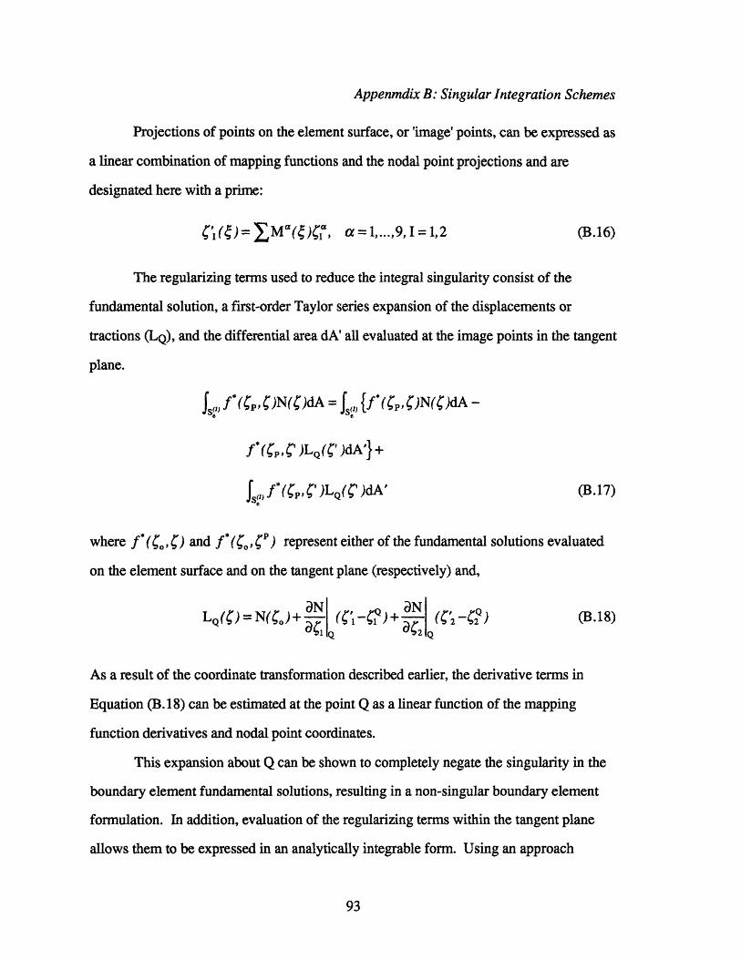
Appenmdix B: Singular Integration Schemes
Projections of points on the element surface, or 'image' points, can be expressed as
a linear combination of mapping functions and the nodal point projections and are
designated here with a prime:
•1 (ý)= M"((r,)a, a = 1,...,9, I = 1,2 (B.16)
The regularizing terms used to reduce the integral singularity consist of the
fundamental solution, a first-order Taylor series expansion of the displacements or
tractions (LQ), and the differential area dA' all evaluated at the image points in the tangent
plane.
f,,f * (( p ', )N ( )d A == js• {f* (ýp, )N(C)dA -
f* (p, ')LQ(' )dA'}+
fs,,f*' (Cp, (')LQ(')dA' (B.17)
where f*(*oC, ') and f*(4, 'P) represent either of the fundamental solutions evaluated
on the element surface and on the tangent plane (respectively) and,
L,(C) = N(C,)+ (' - )•)+ aN(2 (B.18)
As a result of the coordinate transformation described earlier, the derivative terms in
Equation (B.18) can be estimated at the point Q as a linear function of the mapping
function derivatives and nodal point coordinates.
This expansion about Q can be shown to completely negate the singularity in the
boundary element fundamental solutions, resulting in a non-singular boundary element
formulation. In addition, evaluation of the regularizing terms within the tangent plane
allows them to be expressed in an analytically integrable form. Using an approach

Appenmdix B: Singular Integration Schemes
similar to that developed above for fracture solutions, the planar function forms are
converted to a local cylindrical coordinate frame and separated into products of radial and
angular terms. The radial terms are analytically integrated from the origin to the element
boundary image. Finally, the combined angular terms can be integrated using low-order
one-dimensional quadrature.
Although this integration scheme permits evaluation of stress and displacement
fields nearer to the element surface than previously possible, it is not generally the most
cost-effective approach. For source points further from the element than the element
dimension, straightforward two-dimensional numerical integration gives equivalent
results at less expensive.