Thema Working Paper n°2013-32 Université de Cergy Pontoise, France

Regularizing Priors for Linear Inverse Problems

Jean-Pierre Florens Anna Simoni

October, 2013

Regularizing Priors for Linear Inverse Problems*

Jean-Pierre Florens

Toulouse School of Economics

Anna Simoni

CNRS and THEMA

This draft: October 2013

Abstract

This paper proposes a new Bayesian approach for estimating, nonparametrically, functional

parameters in econometric models that are characterized as the solution of a linear inverse

problem. By using a Gaussian process prior distribution we propose the posterior mean as an

estimator and prove frequentist consistency of the posterior distribution. The latter provides the

frequentist validation of our Bayesian procedure. We show that the minimax rate of contraction

of the posterior distribution can be obtained provided that either the regularity of the prior

matches the regularity of the true parameter or the prior is scaled at an appropriate rate.

The scaling parameter of the prior distribution plays the role of a regularization parameter.

We propose a new data-driven method for optimally selecting in practice this regularization

parameter. We also provide sufficient conditions so that the posterior mean, in a conjugate-

Gaussian setting, is equal to a Tikhonov-type estimator in a frequentist setting. Under these

conditions our data-driven method is valid for selecting the regularization parameter of the

Tikhonov estimator as well. Finally, we apply our general methodology to two leading examples

in econometrics: instrumental regression and functional regression estimation.

Key words: nonparametric estimation, Bayesian inverse problems, Gaussian processes, posterior

consistency, data-driven method

JEL code: C13, C11, C14

*First draft: September 2008. A preliminary version of this paper circulated under the title On the Regularization

Power of the Prior Distribution in Linear ill-Posed Inverse Problems. We thank Elise Coudin, Joel Horowitz, EnnoMammen, Andrew Stuart, and Sebastien Van Bellegem for interesting discussions. We also acknowledge helpfulcomments and suggestions from participants to workshops and seminars in Banff (2009), Bressanone (2009), Stats inthe Chateau (Paris 2009), Toulouse (2009), CIRM-Marseille (2009), Brown (2010), Mannheim (2010), Northwestern(2010), World Congress of the Econometric Society (Shangai 2010), Warwick (2011), Cowles Foundation EconometricSummer conference (Yale 2011), Princeton (2012). We thank financial support from ANR-13-BSH1-0004. AnnaSimoni gratefully acknowledges financial support from the University of Mannheim through the DFG-SNF ResearchGroup FOR916, labex MMEDII (ANR11-LBX-0023-01) and hospitality from CREST.

Toulouse School of Economics - 21, allee de Brienne - 31000 Toulouse (France). jean-pierre.florens@tse-fr.euFrench National Center of Scientific Research (CNRS) and THEMA, Universite de Cergy-Pontoise - 33, boulevard

du Port, 95011 Cergy-Pontoise (France). Email: simoni.anna@gmail.com (corresponding author).

1

1 Introduction

In the last decade, econometric theory has shown an increasing interest in the theory of stochas-

tic inverse problems as a fundamental tool for functional estimation of structural as well as reduced

form models. This paper develops an encompassing Bayesian approach to nonparametrically esti-

mate econometric models based on stochastic linear inverse problems.

We construct a Gaussian process prior for the (functional) parameter of interest and estab-

lish sufficient conditions for frequentist consistency of the corresponding posterior mean estimator.

We prove that these conditions are also sufficient to guarantee that the posterior mean estima-

tor numerically equals a Tikhonov-type estimator in the frequentist setting. We propose a novel

data-driven method, based on an empirical Bayes procedure, for selecting the regularization pa-

rameter necessary to implement our Bayes estimator. We show that the value selected by our

data-driven method is optimal in a minimax sense if the prior distribution is sufficiently smooth.

Due to the equivalence between Bayes and Tikhonov-type estimator our data-driven method has

broad applicability and allows to select the regularization parameter necessary for implementing

Tikhonov-type estimators.

Stochastic linear inverse problems theory has recently gained importance in many subfields of

econometrics to construct new estimation methods. Just to mention some of them, it has been

shown to be fundamental in nonparametric estimation of an instrumental regression function, see

e.g. Florens (2003), Newey and Powell (2003), Hall and Horowitz (2005), Blundell et al. (2007),

Darolles et al. (2011), Florens and Simoni (2012a). It has also been used in semiparametric

estimation under moment restrictions, see e.g. Carrasco and Florens (2000), Ai and Chen (2003),

Chen and Pouzo (2012). In addition, it has been exploited for inference in econometric models

with heterogeneity – e.g. Gautier and Kitamura (2012), Hoderlein et al. (2013) – for inference

in auction models – e.g. Florens and Sbaı (2010) – and for frontier estimation for productivity

analysis – e.g. Daouia et al. (2009). Finally, inverse problem theory has been used for functional

regression estimation by e.g. Hall and Horowitz (2007) and Johannes (2008). We refer to Carrasco

et al. (2007) and references therein for a general overview of inverse problems in econometrics.

The general framework used in this paper, and that accommodates many functional estima-

tion problems in econometrics just as mentioned above, is the following. Let X and Y be infinite

dimensional separable Hilbert spaces over R and denote by x ∈ X the functional parameter that

we want to estimate. For instance, x can be an Engel curve or the probability density function

of the unobserved heterogeneity. The estimating equation characterizes x as the solution of the

functional equation

yδ = Kx+ U δ, x ∈ X , yδ ∈ Y, δ > 0 (1)

where yδ is an observable function, K : X → Y is a known, bounded, linear operator and U δ is an

error term with values in Y and covariance operator proportional to a positive scalar δ. Estimating

2

x is an inverse problem. The function yδ is a transformation of a n-sample of finite dimensional

objects and the parameter δ−1 > 0 represents the “level of information” (or precision) of the

sample, so that δ → 0 as n → ∞. For δ = 0 (i.e. perfect information) we have y0 = Kx and

U0 = 0. In many econometric models, equation (1) corresponds to a set of moment equations with

yδ an empirical conditional moment and δ = 1n . A large class of econometric models write under

the form of equation (1) – like moment equality models, consumption based asset pricing models,

density estimation of the heterogeneity parameter in structural models, deconvolution in structural

models with measurement errors. We illustrate two leading examples that can be estimated with

our Bayesian method.

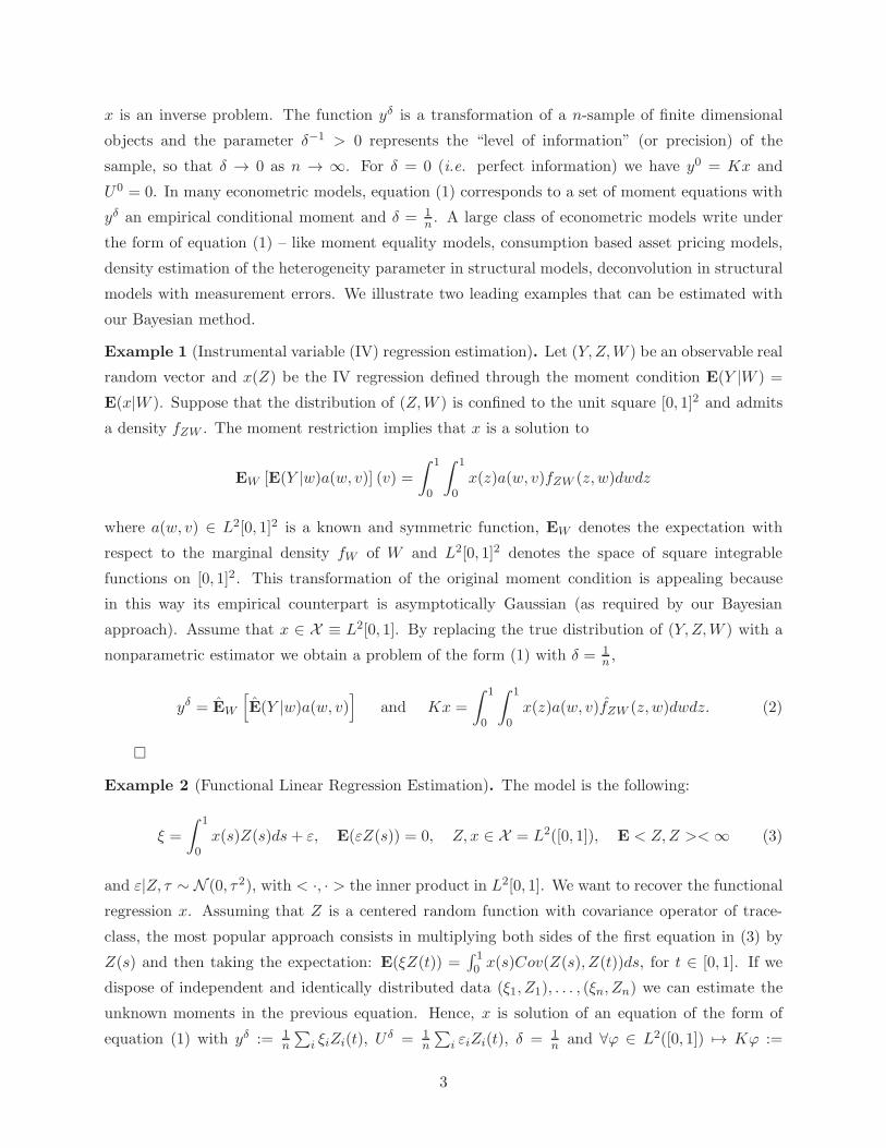
Example 1 (Instrumental variable (IV) regression estimation). Let (Y,Z,W ) be an observable real

random vector and x(Z) be the IV regression defined through the moment condition E(Y |W ) =

E(x|W ). Suppose that the distribution of (Z,W ) is confined to the unit square [0, 1]2 and admits

a density fZW . The moment restriction implies that x is a solution to

EW [E(Y |w)a(w, v)] (v) =∫ 1

0

∫ 1

0x(z)a(w, v)fZW (z, w)dwdz

where a(w, v) ∈ L2[0, 1]2 is a known and symmetric function, EW denotes the expectation with

respect to the marginal density fW of W and L2[0, 1]2 denotes the space of square integrable

functions on [0, 1]2. This transformation of the original moment condition is appealing because

in this way its empirical counterpart is asymptotically Gaussian (as required by our Bayesian

approach). Assume that x ∈ X ≡ L2[0, 1]. By replacing the true distribution of (Y,Z,W ) with a

nonparametric estimator we obtain a problem of the form (1) with δ = 1n ,

yδ = EW

[E(Y |w)a(w, v)

]and Kx =

∫ 1

0

∫ 1

0x(z)a(w, v)fZW (z, w)dwdz. (2)

Example 2 (Functional Linear Regression Estimation). The model is the following:

ξ =

∫ 1

0x(s)Z(s)ds + ε, E(εZ(s)) = 0, Z, x ∈ X = L2([0, 1]), E < Z,Z ><∞ (3)

and ε|Z, τ ∼ N (0, τ2), with < ·, · > the inner product in L2[0, 1]. We want to recover the functional

regression x. Assuming that Z is a centered random function with covariance operator of trace-

class, the most popular approach consists in multiplying both sides of the first equation in (3) by

Z(s) and then taking the expectation: E(ξZ(t)) =∫ 10 x(s)Cov(Z(s), Z(t))ds, for t ∈ [0, 1]. If we

dispose of independent and identically distributed data (ξ1, Z1), . . . , (ξn, Zn) we can estimate the

unknown moments in the previous equation. Hence, x is solution of an equation of the form of

equation (1) with yδ := 1n

∑i ξiZi(t), U

δ = 1n

∑i εiZi(t), δ = 1

n and ∀ϕ ∈ L2([0, 1]) 7→ Kϕ :=

3

1n

∑i < Zi, ϕ > Zi(t).

A Bayesian approach to stochastic inverse problems combines the prior and sampling infor-

mation and proposes the posterior distribution as solution. It allows to deal with two important

issues. First, it allows to incorporate in the estimation procedure the prior information about

the functional parameter provided by the economic theory or the beliefs of experts. This prior

information may be particularly valuable in functional estimation since often the data available are

concentrated only in a region of the graph of the functional parameter so that some parts of the

function can not be recovered from the data.

Second, since the quality of the estimation of the solution of the inverse problem (1) relies on

the value of a regularization parameter, it is particularly important to choose such a parameter in

an accurate way. This can be done with our Bayesian approach.

The majority of the Bayesian approaches to stochastic inverse problems proposed so far are

based on a finite approximation of (1) and so, cannot be applied to functional estimation in econo-

metrics, see e.g. Chapter 5 in Kaipio and Somersalo (2004) and Helin (2009), Lassas et al. (2009),

Hofinger and Pikkarainen (2007), Hofinger and Pikkarainen (2007), Neubauer and Pikkarainen

(2008). These papers consider a finite dimensional projection of (1) and recover x only on a finite

grid of points. Hence, they do not work for econometric models that consider functional obser-

vations and parameters. Knapik et al. (2011) study Bayesian inverse problems with functional

observations and parameter. However, their framework does not allow to accommodate the econo-

metric models of interest because of the different definition of the error term U δ. Indeed, the

analysis of Knapik et al. (2011) works under the assumption that U δ is an isonormal Gaussian

process, which implies that U δ, and by consequence yδ, is not realizable as a random element in

Y. This assumption greatly simplifies the analysis but unfortunately does not hold, in general, in

econometric models because real (functional) data cannot be generated by an isonormal Gaussian

process. On the contrary, our paper works in the more realistic situation where U δ, and therefore

yδ, are random elements with realizations in Y. Thus, our approach works for econometric models.

For the special case where model (1) results from a conditional moment restricted model, Liao

and Jiang (2011) proposed a quasi-Bayesian procedure. Their approach, which works also in the

nonlinear case, is based on limited-information-likelihood and a sieve approximation technique. It

is essentially different from our approach since we work with Gaussian process priors and do not

use a finite-dimensional approximation.

Working with Gaussian process priors is computationally convenient since in many cases

the sampling distribution is (asymptotically) Gaussian and thus the posterior is also Gaussian

(conjugate-Gaussian setting). The current paper gives sufficient conditions under which the pos-

terior mean of x, in a conjugate-Gaussian setting, exists in a closed-form and thus can be used to

estimate x. Existence of such a closed-form is not verified in general, as we explain in the next

4

paragraph and after Theorem 1. Agapiou et al. (2013) propose an alternative approach to deal

with this problem. Florens and Simoni (2012b) overcome this problem by constructing a regu-

larized posterior distribution which works well in practice but the regularization of the posterior

distribution is ad hoc and cannot be justified by any prior-to-posterior transformation. In compar-

ison to Agapiou et al. (2013) and Florens and Simoni (2012b), the current paper also provides an

adaptive method for choosing the regularization parameter as we explain in the next section.

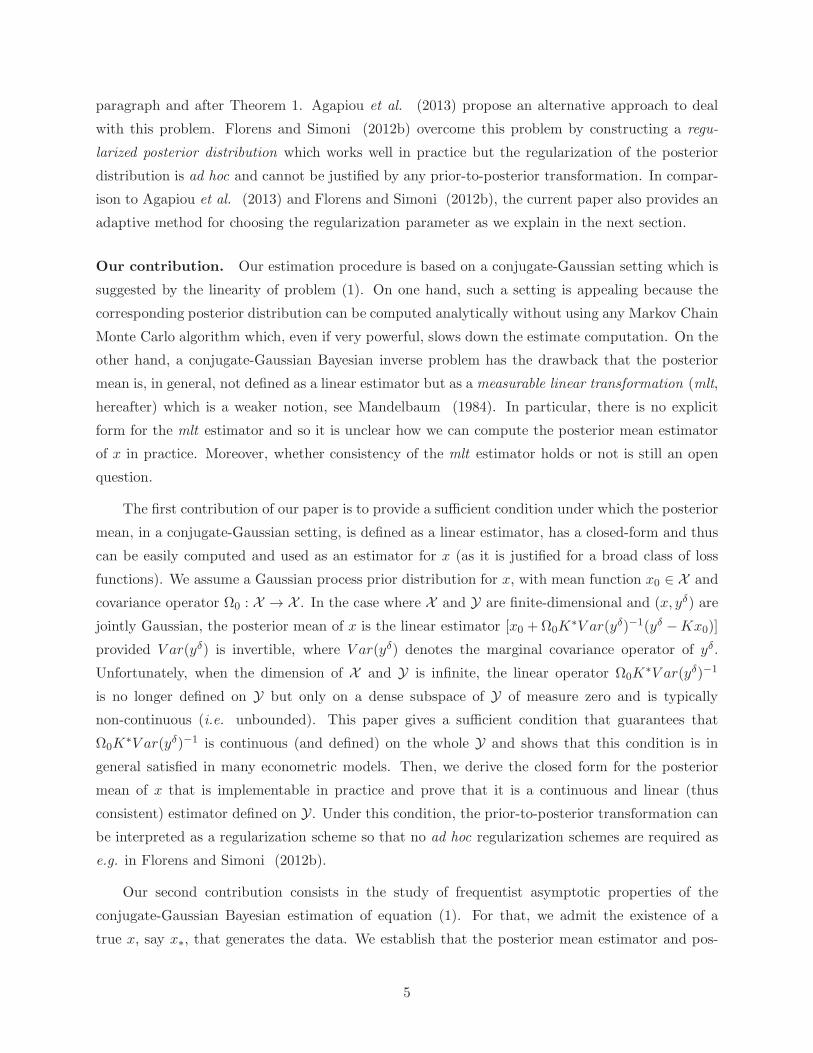
Our contribution. Our estimation procedure is based on a conjugate-Gaussian setting which is

suggested by the linearity of problem (1). On one hand, such a setting is appealing because the

corresponding posterior distribution can be computed analytically without using any Markov Chain

Monte Carlo algorithm which, even if very powerful, slows down the estimate computation. On the

other hand, a conjugate-Gaussian Bayesian inverse problem has the drawback that the posterior

mean is, in general, not defined as a linear estimator but as a measurable linear transformation (mlt,

hereafter) which is a weaker notion, see Mandelbaum (1984). In particular, there is no explicit

form for the mlt estimator and so it is unclear how we can compute the posterior mean estimator

of x in practice. Moreover, whether consistency of the mlt estimator holds or not is still an open

question.

The first contribution of our paper is to provide a sufficient condition under which the posterior

mean, in a conjugate-Gaussian setting, is defined as a linear estimator, has a closed-form and thus

can be easily computed and used as an estimator for x (as it is justified for a broad class of loss

functions). We assume a Gaussian process prior distribution for x, with mean function x0 ∈ X and

covariance operator Ω0 : X → X . In the case where X and Y are finite-dimensional and (x, yδ) are

jointly Gaussian, the posterior mean of x is the linear estimator [x0 +Ω0K∗V ar(yδ)−1(yδ −Kx0)]

provided V ar(yδ) is invertible, where V ar(yδ) denotes the marginal covariance operator of yδ.

Unfortunately, when the dimension of X and Y is infinite, the linear operator Ω0K∗V ar(yδ)−1

is no longer defined on Y but only on a dense subspace of Y of measure zero and is typically

non-continuous (i.e. unbounded). This paper gives a sufficient condition that guarantees that

Ω0K∗V ar(yδ)−1 is continuous (and defined) on the whole Y and shows that this condition is in

general satisfied in many econometric models. Then, we derive the closed form for the posterior

mean of x that is implementable in practice and prove that it is a continuous and linear (thus

consistent) estimator defined on Y. Under this condition, the prior-to-posterior transformation can

be interpreted as a regularization scheme so that no ad hoc regularization schemes are required as

e.g. in Florens and Simoni (2012b).

Our second contribution consists in the study of frequentist asymptotic properties of the

conjugate-Gaussian Bayesian estimation of equation (1). For that, we admit the existence of a

true x, say x∗, that generates the data. We establish that the posterior mean estimator and pos-

5

terior distribution have good frequentist asymptotic properties for δ → 0. More precisely, we show

that the posterior distribution converges towards a Dirac mass at x∗ almost surely with respect to

the sampling distribution (frequentist posterior consistency, see e.g. Diaconis and Freedman (1986,

1998)). This property provides the frequentist validation of our Bayesian procedure.

We also recover the rate of contraction of the risk associated with the posterior mean and of

the posterior distribution. This rate depends on the smoothness and the scale of the prior as well

as on the smoothness of x∗. Depending on the specification of the prior this rate may be minimax

over a Sobolev ellipsoid. In particular, (i) when the regularity of the prior matches the regularity

of x∗, the minimax rate of convergence is obtained with a fixed prior covariance; (ii) when the prior

is rougher or smoother at any degree than the truth, the minimax rate can still be obtained if the

prior is scaled at an appropriate rate depending on the unknown regularity of x∗.

Our third contribution consists in proposing a new data-driven method for optimally selecting

the regularization parameter. This parameter enters the prior distribution as a scaling hyperpa-

rameter of the prior covariance and is needed to compute the posterior mean of x. Our adaptive

data-driven method is based on an empirical Bayes (EB) approach. Because the posterior mean

is, under our assumptions, equal to a Tikhonov-type estimator for problem (1), our EB approach

for selecting the regularization parameter is valid, and can be used, also for computing frequentist

estimators based on Tikhonov regularization.1 Finally, the EB-selected regularization parameter

is plugged into the prior distribution of x and for the corresponding EB-posterior distribution we

prove frequentist posterior consistency.

In the following, we present the Bayesian approach and the asymptotic results for general

models of the form (1); then, we develop further results that apply to the specific examples 1 and 2.

In section 2 we set the Bayesian model associated with (1) and the main assumptions. In section 3

the posterior distribution of x is computed and its frequentist asymptotic properties are analyzed.

Section 4 focuses on the mildly ill-posed case. The EB method is developed in section 5. Section

6 shows numerical implementations and section 7 concludes. All the proofs are in the Appendix.

2 The Model

Let X and Y be infinite dimensional separable Hilbert spaces over R with norm || · || inducedby the inner product < ·, · >. Let B(X ) and B(Y) be the Borel σ-fields generated by the open sets

of X and Y, respectively. We consider the inverse problem of estimating the function x ∈ X which

1Notice that in general the posterior mean in a conjugate-Gaussian problem stated in infinite-dimensional Hilbertspaces cannot be equal to the Tikhonov solution of (1). This is due to the particular structure of the covarianceoperator of the error term Uδ and it will be detailed in section 2.

6

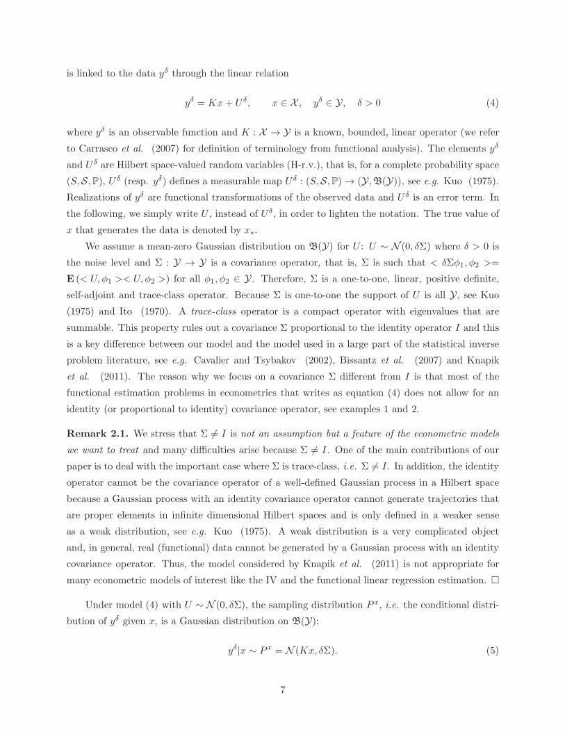
is linked to the data yδ through the linear relation

yδ = Kx+ U δ, x ∈ X , yδ ∈ Y, δ > 0 (4)

where yδ is an observable function and K : X → Y is a known, bounded, linear operator (we refer

to Carrasco et al. (2007) for definition of terminology from functional analysis). The elements yδ

and U δ are Hilbert space-valued random variables (H-r.v.), that is, for a complete probability space

(S,S,P), U δ (resp. yδ) defines a measurable map U δ : (S,S,P) → (Y,B(Y)), see e.g. Kuo (1975).

Realizations of yδ are functional transformations of the observed data and U δ is an error term. In

the following, we simply write U , instead of U δ, in order to lighten the notation. The true value of

x that generates the data is denoted by x∗.

We assume a mean-zero Gaussian distribution on B(Y) for U : U ∼ N (0, δΣ) where δ > 0 is

the noise level and Σ : Y → Y is a covariance operator, that is, Σ is such that < δΣφ1, φ2 >=

E (< U,φ1 >< U,φ2 >) for all φ1, φ2 ∈ Y. Therefore, Σ is a one-to-one, linear, positive definite,

self-adjoint and trace-class operator. Because Σ is one-to-one the support of U is all Y, see Kuo

(1975) and Ito (1970). A trace-class operator is a compact operator with eigenvalues that are

summable. This property rules out a covariance Σ proportional to the identity operator I and this

is a key difference between our model and the model used in a large part of the statistical inverse

problem literature, see e.g. Cavalier and Tsybakov (2002), Bissantz et al. (2007) and Knapik

et al. (2011). The reason why we focus on a covariance Σ different from I is that most of the

functional estimation problems in econometrics that writes as equation (4) does not allow for an

identity (or proportional to identity) covariance operator, see examples 1 and 2.

Remark 2.1. We stress that Σ 6= I is not an assumption but a feature of the econometric models

we want to treat and many difficulties arise because Σ 6= I. One of the main contributions of our

paper is to deal with the important case where Σ is trace-class, i.e. Σ 6= I. In addition, the identity

operator cannot be the covariance operator of a well-defined Gaussian process in a Hilbert space

because a Gaussian process with an identity covariance operator cannot generate trajectories that

are proper elements in infinite dimensional Hilbert spaces and is only defined in a weaker sense

as a weak distribution, see e.g. Kuo (1975). A weak distribution is a very complicated object

and, in general, real (functional) data cannot be generated by a Gaussian process with an identity

covariance operator. Thus, the model considered by Knapik et al. (2011) is not appropriate for

many econometric models of interest like the IV and the functional linear regression estimation.

Under model (4) with U ∼ N (0, δΣ), the sampling distribution P x, i.e. the conditional distri-

bution of yδ given x, is a Gaussian distribution on B(Y):

yδ|x ∼ P x = N (Kx, δΣ). (5)

7

The parameter δ > 0 is assumed to converge to 0 when the information from the observed data

increases. Hereafter, Ex(·) will denote the expectation taken with respect to P x.

Remark 2.2. The assumption of Gaussianity of the error term U in the econometric model (4)

is not necessary and only made in order to construct (and give a Bayesian interpretation to) the

estimator. The proofs of our results of frequency consistency do not rely on the normality of U .

In particular, asymptotic normality of yδ|x, which is verified e.g. in example 1, is enough for

our estimation procedure and also for our EB data-driven method for choosing the regularization

parameter.

Remark 2.3. All the results in the paper are given for the general case where K and Σ do not

depend on δ. This choice is made in order to keep our presentation as simple as possible. We

discuss how our results apply to the case with unknown K and Σ through examples 1 and 2.

2.1 Notation

We set up some notational convention used in the paper. We simply write U to denote the

error term U δ. For positive quantities Mδ and Nδ depending on a discrete or continuous index δ,

we write Mδ ≍ Nδ to mean that the ratio Mδ/Nδ is bounded away from zero and infinity. We

write Mδ = O(Nδ) if Mδ is at most of the same order as Nδ. For an H-r.v. W we write W ∼ Nfor denoting that W is a Gaussian process. We denote by R(·) the range of an operator and

by D(·) its domain. For an operator B : X → Y, R(B) denotes the closure in Y of the range

of B. For a bounded operator A : Y → X , we denote by A∗ its adjoint, i.e. A∗ : X → Y is

such that < Aψ,ϕ >=< ψ,A∗ϕ >, ∀ ϕ ∈ X , ψ ∈ Y. The operator norm is defined as ||A|| :=sup||φ||=1 ||Aφ|| = minC ≥ 0 ; ||Aφ|| ≤ C||φ|| for all φ ∈ Y. The operator I denotes the identity

operator on both spaces X and Y, i.e. ∀ψ ∈ X , ϕ ∈ Y, Iψ = ψ and Iϕ = ϕ.

Let ϕjj denote an orthonormal basis of Y. The trace of a bounded linear operator A : Y → Xis defined as tr(A) :=

∑∞j=1 < (A∗A)

12ϕj , ϕj > independently of the basis ϕjj. If A is compact

then its trace writes tr(A) =∑∞

j=1 λj , where λj are the singular values of A. The Hilbert-

Schmidt norm of a bounded linear operator A : Y → X is denoted by ||A||HS and defined as

||A||2HS = tr(A∗A), see Kato (1995).

2.2 Prior measure and main assumptions

In this section we introduce the prior distribution and two sets of assumptions. (i) The first set

(Assumptions A.2 and B below) will be used for establishing the rate of contraction of the posterior

distribution and concerns the smoothness of the operator Σ−1/2K and of the true value x∗. (ii) The

assumptions in the second set (A.1 and A.3 below) are new in the literature and guarantee continuity

of the posterior mean of x as a linear operator on Y. The detection of the latter assumptions is

8

an important contribution because, as remarked in Luschgy (1995) and Mandelbaum (1984),

in the Gaussian infinite-dimensional model the posterior mean is in general only defined as a mlt

which is a weaker notion than that one of a continuous linear operator. Therefore, in general the

posterior mean has not an explicit form and may be an inconsistent estimator in the frequentist

sense while our Assumptions A.1 and A.3 ensure closed-form (easy to compute) and consistency

for the posterior mean.

Assumption A.1. R(K) ⊂ D(Σ−1/2).

Since K and Σ are integral operators, Σ−1/2 is a differential operator and Assumption A.1

demands that the functions in R(K) are at least as smooth as the functions in R(Σ1/2). A.1

ensures that Σ−1/2 is defined on R(K) so that Σ−1/2K, which is used in Assumption A.2, exists.

Assumption A.2. There exists an unbounded, self-adjoint, densely defined operator L in the

Hilbert space X for which ∃ η > 0 such that < Lψ,ψ >≥ η||ψ||2, ∀ψ ∈ D(L), and that satisfies

m||L−ax|| ≤ ||Σ−1/2Kx|| ≤ m||L−ax|| (6)

on X for some a > 0 and 0 < m ≤ m <∞. Moreover, L−2s is trace-class for some s > a.

Assumption A.2 means that Σ−1/2K regularizes at least as much as L−a. Because Σ−1/2K

must satisfy (6) it is necessarily an injective operator.

We turn now to the construction of the prior distribution of x. Our proposal is to use the

operator L−2s to construct the prior covariance operator. We assume a Gaussian prior distribution

µ on B(X ):

x|α, s ∼ µ = N(x0,

δ

αΩ0

), x0 ∈ X , Ω0 := L−2s, s > a (7)

with α > 0 such that α→ 0 as δ → 0. The parameter α describes a class of prior distributions and

it may be viewed as an hyperparameter. Section 5 provides an EB approach for selecting it.

By definition of L, the operator Ω0 : X → X is linear, bounded, positive-definite, self-adjoint,

compact and trace-class. It results evident from Assumption A.2 that such a choice for the prior

covariance is aimed at linking the prior distribution to the sampling model. A similar idea was

proposed by Zellner (1986) for linear regression models for which he constructed a class of prior

called g-prior. Our prior (7) is an extension of the Zellner’s g-prior and we call it extended g-prior.

The distribution µ (resp. P x) is realizable as a proper random element in X (resp. Y) if

and only if Ω0 (resp. Σ) is trace-class. Thus, neither Σ nor Ω0 can be proportional to I so that,

in general, in infinite-dimensional inverse problems, the posterior mean cannot be equal to the

Tikhonov regularized estimator xTα := (αI +K∗K)−1K∗yδ. However, we show in this paper that

under A.1, A.2 and A.3, the posterior mean equals the Tikhonov regularized solution in the Hilbert

Scale generated by L. We give later the definition of Hilbert Scale.

9

The following assumption ties further the prior to the sampling distribution by linking the

smoothing properties of Σ, K and Ω120 .

Assumption A.3. R(KΩ120 ) ⊂ D(Σ−1).

Hereafter, we denote B = Σ−1/2KΩ120 . Assumption A.3 guarantees that B and Σ−1/2B exist.

We now discuss the relationship between Assumption A.2, which quantifies the smoothness of

Σ−1/2K, and Assumption B below, which quantifies the smoothness of the true value x∗. In order

to explain these assumptions and their link we will: (i) introduce the definition of Hilbert scale, (ii)

explain the meaning of the parameter a in (6), (iii) discuss the smoothness conditions of Σ−1/2K

and of the true value of x.

(i) The operator L in Assumption A.2 is a generating operator of the Hilbert scale (Xt)t∈R

where ∀t ∈ R, Xt is the completion of⋂

k∈RD(Lk) with respect to the norm ||x||t := ||Ltx|| and is

a Hilbert space, see Definition 8.18 in Engl et al. (2000), Goldenshluger and Pereverzev (2003)

or Krein and Petunin (1966). For t > 0 the space Xt ⊂ X is the domain of definition of Lt:

Xt = D(Lt). Typical examples of Xt are Sobolev spaces of various kinds.

(ii) We refer to the parameter a in A.2 as the “degree of ill-posedness” of the estimation

problem under study and a is determined by the rate of decreasing of the spectrum of Σ−1/2K

(and not only by that one of K as it would be in a classical inverse problems framework for (1)).

Since the spectrum of Σ−1/2K is decreasing slower than that one of K we have to control for less

ill-posedness than if we used the classical approach.

(iii) In inverse problems theory it is natural to impose conditions on the regularity of x∗ by

relating it to the regularity of the operator that characterizes the inverse problem (that is, the

operator Σ−1/2K in our case). A possible implementation of this consists in introducing a Hilbert

Scale and expressing the regularity of both x∗ and Σ−1/2K with respect to this common Hilbert

Scale. This is the meaning of - and the link between - Assumptions A.2 and B where we use the

Hilbert Scale (Xt)t∈R generated by L. We refer to Chen and Reiss (2011) and Johannes et al.

(2011) for an explanation of the relationship between Hilbert Scale and regularity conditions. The

following assumption expresses the regularity of x∗ according to Xt.

Assumption B. For some 0 ≤ β, (x∗ − x0) ∈ Xβ, that is, there exists a ρ∗ ∈ X such that

(x∗ − x0) = L−βρ∗ (≡ Ωβ2s0 ρ∗).

The parameter β characterizes the “regularity” of the centered true function (x∗ − x0) and is

generally unknown. Assumption B is satisfied by regular functions x∗. In principle, it could be

satisfied also by irregular x∗ if we were able to decompose x∗ in the sum of a regular part plus

an irregular part and to choose x0 such that it takes all the irregularity of x∗. This is clearly

infeasible in practice as x∗ is unknown. On the contrary, we could choose a very smooth function

x0 so that Assumption B would be less demanding about the regularity of x∗. When Xβ is the

10

scale of Sobolev spaces, Assumption B is equivalent to assume that (x∗ − x0) has at least β square

integrable derivatives.

Assumption B is classical in inverse problems literature, see e.g. Chen and Reiss (2011) and

Nair et al. (2005), and is closely related to the so-called source condition which expresses the

regularity of x∗ according to the spectral representation of the operator K∗K defining the inverse

problem, see Engl et al. (2000) and Carrasco et al. (2007). In our case, the regularity of (x∗−x0)is expressed according to the spectral representation of L.

Remark 2.4. Assumption A.2 covers not only the mildly ill-posed but also the severely ill-posed

case if (x∗ − x0) in Assumption B is infinitely smooth. In the mildly ill-posed case the singular

values of Σ−1/2K decay slowly to zero (typically at a geometric rate) which means that the kernel

of Σ−1/2K is finitely smooth. In this case the operator L is generally some differential operator

so that L−1 is finitely smooth. In the severely ill-posed case the singular values of Σ−1/2K decay

very rapidly (typically at an exponential rate). Assumption A.2 covers also this case if (x∗ − x0) is

very smooth. This is because when the singular values of Σ−1/2K decay exponentially, Assumption

A.2 is satisfied if L−1 has an exponentially decreasing spectrum too. On the other hand, L−1

is used to describe the regularity of (x∗ − x0), so that in the severely ill-posed case, Assumption

B can be satisfied only if (x∗ − x0) is infinitely smooth. In this case we could for instance take

L = (K∗Σ−1K)−12 which implies a = 1. We could make Assumption A.2 more general, as in Chen

and Reiss (2011), in order to cover the severely ill-posed case even when (x∗ − x0) is not infinitely

smooth. Since computations to find the rate would become more cumbersome (even if still possible)

we do not pursue this direction here.

Remark 2.5. The specification of the prior covariance operator can be generalized as δαΩ0 =

δαQL

−2sQ∗, for some bounded operator Q not necessarily compact. Then, the previous case is a

particular case of this one for Q = I. In this setting, Assumptions A.1 and A.3 are replaced by the

weaker assumptions R(KQ) ⊂ D(Σ−1/2) and R(KQL−s) ⊂ D(Σ−1), respectively. In Assumption

A.2 the operator Σ−1/2K must be replaced by Σ−1/2KQ and Assumption B becomes: there exists

ρ∗ ∈ X such that (x∗ − x0) = QL−β ρ∗.

Example 1 (Instrumental variable (IV) regression estimation (continued)). Let us consider the

integral equation (4), with yδ and K defined as in (2), that characterizes the IV regression x.

Suppose to use the kernel smoothing approach to estimate fYW and fZW , where fYW denotes

the density of the distribution of (Y,W ) with respect to the Lebesgue measure. For simplicity we

assume that (Z,W ) is a bivariate random vector. Let KZ,h and KW,h denote two univariate kernel

functions in L2[0, 1], h be the bandwidth and (yi, wi, zi)ni=1 be the n-observed random sample.

Denote Λ : L2[0, 1] → L2[0, 1] the operator Λϕ =∫a(w, v)ϕ(w)dw, with a(w, v) a known function,

and K : L2[0, 1] → L2[0, 1] the operator Kφ = 1n

∑ni=1

KW,h(wi−w)h < φ(z),

KZ,h(zi−z)h >. Therefore,

11

K = ΛK so that the quantities in (2) can be rewritten as

yδ = Λ[E(Y |W = w)fW

](v) =

∫a(w, v)

1

nh

n∑

i=1

yiKW,h(wi − w)dw

and Kx =

∫a(w, v)

1

n

n∑

i=1

KW,h(wi − w)

h

∫x(z)

KZ,h(zi − z)

hdzdw (8)

Remark that limn→∞ Kφ = fW (w)E(φ|w) = MfE(φ|w) where Mf denotes the multiplication op-

erator by fW . If a = fWZ then Λ limn→∞ K is the same integral operator in Hall and Horowitz

(2005).

In this example, the assumption that U ∼ N (0, δΣ) (where U = yδ−Kx) holds asymptotically

and the transformation of the model through Λ is necessary in order to guarantee such a convergence

of U towards a zero-mean Gaussian process. We explain this fact by extending Ruymgaart (1998).

It is possible to show that the covariance operator Σh of√nn

∑ni=1

(yi− < x,

KZ,h(zi−z)h >

)KW,h(wi−w)

h

satisfies

< φ1, Σhφ2 > −→ < φ1, Σφ2 >, as h→ 0, ∀φ1, φ2 ∈ L2[0, 1]

where Σφ2 = σ2fW (v)φ2(v) = σ2Mfφ2(v) under the assumption E[(Y − x(Z))2|W ] = σ2 < ∞.

Unfortunately, because Σ has not finite trace, it is incompatible with the covariance structure of a

Gaussian limiting probability measure. The result is even worst, since Ruymgaart (1998) shows

that there are no scaling factors n−r, for 0 < r < 1, such that n−r∑n

i=1

(yi− < x,

KZ,h(zi−z)h >

)×

KW,h(wi−w)h converges weakly in L2[0, 1] to a Gaussian distribution (unless this distribution is de-

generate at the zero function). However, if we choose a(w, v) appropriately so that Λ is a compact

operator and Λ∗Λ has finite trace, then√n(yδ −Kx

)⇒ N (0,ΛΣΛ∗), in L2[0, 1] as n→ ∞, where

‘⇒’ denotes weak convergence and ΛΣΛ∗ =: Σ. The adjoint operator Λ∗ : L2[0, 1] → L2[0, 1] is

defined as: ∀ϕ ∈ L2[0, 1], Λ∗ϕ =∫a(w, v)ϕ(v)dv and Λ = Λ∗ if a(w, v) is symmetric in w and v.

The operator Σ is unknown and can be estimated by Σ = Λ σ2

n

∑ni=1

KW,h(wi−w)h Λ∗.

We now discuss Assumptions A.1, A.2 and A.3. While A.1 and A.3 need to hold both in

finite sample and for n → ∞, A.2 only has to hold for n → ∞. We start by checking As-

sumption A.1. In large sample, the operator K converges to ΛMfE(φ|w) and it is trivial to

verify that D(Σ−1/2) = R(ΛM12f ) ⊃ R(ΛMf ) ⊃ R(ΛMfE(·|w)). In finite sample, the same holds

with Mf and E(·|w) replaced by their empirical counterparts. Next, we check the validity of As-

sumption A.2 for n → ∞. Remark that the operator Σ1/2 may be equivalently defined in two

ways: (1) as a self-adjoint operator, that is Σ1/2 = (Σ1/2)∗ = (ΛMfΛ∗)1/2, so that Σ = Σ1/2Σ1/2

or (2) as Σ1/2 = ΛM1/2f so that Σ = Σ1/2(Σ1/2)∗ where (Σ1/2)∗ = M

12f Λ

∗. By using the sec-

ond definition, we obtain that Σ−1/2K = (ΛM12f )

−1ΛK = f− 1

2W Λ−1ΛK = f

− 12

W K and ∀x ∈ X ,

|| limn→∞Σ−1/2Kx|| = ||E(x|w)||2W , where ||φ||2W :=∫[φ(w)]2fW (w)dw. This shows that, in the

IV case, Assumption A.2 is a particular case of Assumptions 2.2 and 4.2 in Chen and Reiss (2011).

12

Finally, we check Assumption A.3 for both n → ∞ and finite sample. In finite sample this

assumption holds trivially since R(Σ) (≡ D(Σ−1)) and R(KΩ120 ) have finite ranks. Suppose that

the conditions for the application of the Dominated Convergence Theorem hold, then Assumption

A.3 is satisfied asymptotically if and only if ||Σ−1Λ limn→∞ KΩ120 ||2 < ∞. This holds if Ω0 is ap-

propriately chosen. One possibility could be to set Ω0 = T ∗Λ∗ΛT , where T : L2[0, 1] → L2[0, 1] is

a trace-class integral operator Tφ =∫ω(w, z)φ(z)dz for a known function ω and T ∗ is its adjoint.

Define Ω120 = T ∗Λ∗. Then,2

||Σ−1Λ limn→∞

KΩ120 ||2 = ||Σ−1Λ lim

n→∞KT ∗Λ∗||2 ≤ ||Σ−1Λ lim

n→∞KT ∗Λ∗||2HS ≤ tr(Σ−1Λ lim

n→∞KT ∗Λ∗)

= tr(Λ∗Σ−1Λ limn→∞

KT ∗) = tr(E(T ∗ · |w)) ≤ tr(T ∗)||E(·|W )|| <∞.

2.2.1 Covariance operators proportional to K

A particular situation often encountered in applications is the case where the sampling covari-

ance operator has the form Σ = (KK∗)r, for some r ∈ R+, and is related to the classical example

of g-priors given in Zellner (1986). In this situation it is convenient to choose L = (K∗K)−12 so

that Ω0 = (K∗K)s, for s ∈ R+. Because (KK∗)r and (K∗K)s are proper covariance operators only

if they are trace-class then K is necessarily compact. Assumptions A.1 and A.2 hold for r ≤ 1 and

a = 1− r, respectively. Assumption A.3 holds for s ≥ 2r − 1.

Example 2 (Functional Linear Regression Estimation (continued)). Let us consider model (3) and

the associated integral equation E(ξZ(t)) =∫ 10 x(s)Cov(Z(s), Z(t))ds, for t ∈ [0, 1]. If we dispose

of i.i.d. data (ξ1, Z1), . . . , (ξn, Zn) the unknown moments in this equation can be estimated. Thus,

x is solution of (4) with yδ := 1n

∑i ξiZi(t), U = 1

n

∑i εiZi(t) and ∀ϕ ∈ L2([0, 1]) 7→ Kϕ :=

1n

∑i < Zi, ϕ > Zi(t). The operator K : L2([0, 1]) → L2([0, 1]) is self-adjoint, i.e. K = K∗.

Moreover, conditional on Z, the error term U is exactly a Gaussian process with covariance operator

δΣ = δτ2K with δ = 1n which is trace-class since its range has finite dimension. Thus, we can write

δΣ = 1nτ

2(KK∗)r with r = 12 . Assumption A.1 is trivially satisfied in finite sample as well as for

n→ ∞. We discuss later on how to choose L in order to satisfy Assumptions A.2 and A.3.

2.2.2 Imposing shape restrictions through the Gaussian process prior

We briefly discuss how restrictions such as monotonicity, convexity, or more generally shape

restrictions can be incorporated into a Gaussian process prior, see Berger and Wang (2011) for more

details. First, to be sure that the realizations of a Gaussian process with mean x0 and covariance

operator Ω0 have derivatives of all orders one should take as x0 an infinitely differentiable function

and as kernel of Ω0 a squared exponential covariance function, that is: ω0(t, t) = b1 exp−b2(t− t)2,

2This is because for a compact operator A : L2[0, 1] → L2[0, 1] and by denoting |A| = (A∗A)1/2, we have:||A||2 ≤ ||A||2HS = || |A| ||2HS ≤ tr(|A|) = tr(A).

13

b1 > 0, b2 ≥ 0 where Ω0ϕ =∫ω0(t, t)ϕ(t)dt, ∀ϕ ∈ X .

Second, since differentiation is a linear operator, derivatives of a Gaussian process remain a

Gaussian process. Thus, if x(k) denotes the k-th derivative of x, then x(k) is a Gaussian process

with mean x(k)0 and covariance operator Ωkk with kernel σkk(t, t) = ∂2k

∂tk∂tkω0(t, t). Moreover, the

covariance operator between x and x(k) is denoted by Ω0k and has kernel σkk(t, t) =∂k

∂tkω0(t, t). To

incorporate the shape restrictions one should constrain the derivative x(k)(t) at a discrete set of

points t1, . . . , tm (dense enough to guarantee that the realizations of x will satisfy the constraint)

and then fix the prior µ, for x, equal to the conditional distribution of x|x(k)(ti)mi=1, which is

Gaussian. That is, by abuse of notation: x|α, t ∼ µ = N (x0,Ω0) with

x0 = x0 + Ω0kΩ−1kk x(k)(ti)− x

(k)0 (ti)mi=1, Ω0 = Ω0 − Ω0kΩ

−1kk Ωk0

where x(k)(ti)− x(k)0 (ti)mi=1 denotes the m-vector with i-th element x(k)(ti)− x

(k)0 (ti).

3 Main results

The posterior distribution of x, denoted by µYδ , is the Bayesian solution of the inverse problem

(4). Because a separable Hilbert space is Polish, there exists a regular version of the posterior

distribution µYδ , that is, a conditional probability characterizing µYδ . In many applications X and

Y are L2 spaces and L2 spaces are Polish if they are defined on a separable metric space. In the

next theorem we characterize the joint distribution of (x, yδ) and the posterior distribution µYδ of

x. The notation B(X ) ⊗B(Y) means the Borel σ-field generated by the product topology.

Theorem 1. Consider two separable infinite dimensional Hilbert spaces X and Y. Let x|α, s and

yδ|x be two Gaussian H-r.v. on X and Y as in (7) and (5), respectively. Then,

(i) (x, yδ) is a measurable map from (S,S,P) to (X × Y,B(X ) ⊗ B(Y)) and has a Gaussian

distribution: (x, yδ)|α, s ∼ N ((x0,Kx0),Υ), where Υ is a trace-class covariance operator

defined as Υ(ϕ,ψ) =(δαΩ0ϕ+ δ

αΩ0K∗ψ, δ

αKΩ0ϕ+ (δΣ + δαKΩ0K

∗)ψ)for all (ϕ,ψ) ∈ X ×

Y. The marginal sampling distribution of yδ|α, s is Pα ∼ N (Kx0, (δΣ + δαKΩ0K

∗)).

Moreover, let A : Y → X be a Pα-measurable linear transformation (Pα-mlt), that is, ∀φ ∈ Y, Aφis a Pα-almost sure limit, in the norm topology, of Akφ as k → ∞, where Ak : Y → X is a sequence

of continuous linear operators. Then,

(ii) the conditional distribution µYδ of x given yδ exists, is regular and almost surely unique. It

is Gaussian with mean E(x|yδ, α, s) = A(yδ −Kx0) + x0 and trace-class covariance operator

V ar(x|yδ, α, s) = δα [Ω0 − AKΩ0] : X → X . Furthermore, A = Ω0K

∗(αΣ + KΩ0K∗)−1 on

R((δΣ + δαKΩ0K

∗)12 ).

14

(iii) Under Assumptions A.1 and A.3, the operator A characterizing µYδ is a continuous linear

operator on Y and can be written as

A = Ω120 (αI +B∗B)−1(Σ−1/2B)∗ : Y → X (9)

with B = Σ−1/2KΩ120 .

Point (ii) in the theorem is an immediate application of the results of Mandelbaum (1984), we

refer to this paper for the proof and for a rigorous definition of Pα-mlt. As stated above, the quantity

Ayδ is defined as a Pα-mlt, which is a weaker notion than that of a linear and continuous operator

and A is in general not continuous. In fact, since Ayδ is a Pα-almost sure limit of Akyδ, for k → ∞,

the null set where this convergence is not satisfied depends on yδ and we do not have an almost sure

convergence of Ak to A. Moreover, in general, A takes the form A = Ω0K∗(αΣ+KΩ0K

∗)−1 only on

a dense subspace of Y of Pα-probability measure zero. Outside of this subspace, A is defined as the

unique extension of Ω0K∗(αΣ +KΩ0K

∗)−1 to Y for which we do not have an explicit expression.

This means that in general it is not possible to construct a feasible estimator for x.

On the contrary, point (iii) of the theorem shows that, under A.1 and A.3, A is defined as a

continuous linear operator on the whole Y. This is the first important contribution of our paper

since A.1 and A.3 permit to construct a linear estimator for x – equal to the posterior mean –

that is implementable in practice. Thus, our result (iii) makes operational the Bayesian approach

for linear statistical inverse problems in econometrics. When Assumptions A.1 and A.3 do not

hold then we can use a quasi-Bayesian approach as proposed in Florens and Simoni (2012a,b).

Summarizing, under a quadratic loss function, the Bayes estimator for a functional parameter x

characterized by (4) is the posterior mean

xα = Ω120 (αI +B∗B)−1(Σ−1/2B)∗(yδ −Kx0), with B = Σ−1/2KΩ1/2.

Remark 3.1. Under our assumptions it is possible to show the existence of a close relationship

between Bayesian and frequentist approach to statistical inverse problems. In fact, the posterior

mean xα is equal to the Tikhonov regularized solution in the Hilbert scale (Xs)s∈R generated by

L of the equation Σ−1/2yδ = Σ−1/2Kx+ Σ−1/2U . The existence of Σ−1/2K is guaranteed by A.1.

Since E(x|yδ, α, s) = A(yδ −Kx0) + x0, we have, under A.1 and A.3:

E(x|yδ, α, s) = L−s(αI + L−sK∗Σ−1KL−s)−1L−sK∗Σ−1/2Σ−1/2(yδ −Kx0) + x0

= (αL2s + T ∗T )−1T ∗(yδ − Tx0) + x0, where T = Σ−1/2K, yδ = Σ−1/2yδ

and it is equal to the minimizer, with respect to x, of the Tikhonov functional

||yδ − Tx||2 + α||x− x0||2s.

15

The quantities Σ−1/2yδ and Σ−1/2U have to be interpreted in the sense of weak distributions,

see Kuo (1975) and Bissantz et al. (2007). In the IV regression estimation (see Example 1 for the

notation), Σ−1/2yδ = E(Y |W )f12W , Tx = E(x|W )f

12W and the posterior mean estimator writes

xα =

(αL2s + K∗ 1

ˆfWK

)−1

K∗(E(Y − x0|W )

)=(αL2s + E

[E(·|W )|Z

])−1E[E(Y − x0|W )|Z

].

For x0 = 0 this is, in the framework of Darolles et al. (2011) or Florens et al. (2011), the Tikhonov

estimator in the Hilbert scale generated by 1fZL2s.

3.1 Asymptotic analysis

We analyze now frequentist asymptotic properties of the posterior distribution µYδ of x. The

asymptotic analysis is for δ → 0. Let P x∗ denote the sampling distribution (5) with x = x∗, we

remind the definition of posterior consistency, see Diaconis and Freedman (1986) or Ghosh and

Ramamoorthi (2003):

Definition 1. The posterior distribution is consistent at x∗ with respect to P x∗ if it weakly con-

verges towards the Dirac measure δx∗ at the point x∗, i.e. if, for every neighborhood U of x∗,

µYδ (U|yδ, α, s) → 1 in P x∗-probability or P x∗-a.s. as δ → 0.

Posterior consistency provides the basic frequentist validation of our Bayesian procedure be-

cause it ensures that with a sufficiently large amount of data, it is almost possible to recover the

truth accurately. Lack of consistency is extremely undesirable, and one should not use a Bayesian

procedure if the corresponding posterior distribution is inconsistent.

Our asymptotic analysis is organized as follows. First, we consider the posterior mean xα as an

estimator for the solution of (4) and study the rate of convergence of the associated risk. Second,

we state posterior consistency and recover the rate of contraction of the posterior distribution. We

denote the risk (MISE) associated with xα by Ex∗ ||xα − x∗||2 where Ex∗ denotes the expectation

taken with respect to P x∗ . Let λjL denote the eigenvalues of L−1, we define:

γ := infγ ∈ (0, 1] ;

∞∑

j=1

λ2γ(a+s)jL <∞ ≡ infγ ∈ (0, 1] ; tr(L−2γ(a+s)) <∞. (10)

We point out that γ is known since it depends on L. For instance, γ = 12(a+s) means that either L−1

is trace-class but L−(1−ω) is not trace-class for every ω ∈ R+ or that tr(L−(1+ω)

)< ∞, ∀ω ∈ R+

but L−1 is not trace-class. Since under A.2 the operator L−2s is trace-class, the parameter γ

cannot be larger than sa+s . Thus, if γ = 1

2(a+s) this implies that s ≥ 12 since 1

2(a+s) must be less

than or equal to s(a+s) . Remark that the smaller the γ is and the smaller the eigenvalues of L−1

16

are. Furthermore, we denote by Xβ(Γ) the ellipsoid of the type

Xβ(Γ) := ϕ ∈ X ; ||ϕ||2β ≤ Γ, 0 < Γ <∞ (11)

where ||ϕ||β := ||Lβϕ||. Our asymptotic results will be valid uniformly on Xβ(Γ). The following

theorem gives the asymptotic behavior of xα.3

Theorem 2. Let us consider the observational model (4) with x∗ being the true value of x that

generates the data. Under Assumptions A.1-A.3 and B, we have

sup(x∗−x0)∈Xβ(Γ)

Ex∗||xα − x∗||2 = O(α

βa+s + δα− a+γ(a+s)

a+s

)

with β = min(β, a + 2s).

The theorem provides an uniform rate over the ellipsoid Xβ(Γ). It follows from this result that

if (x∗ − x0) satisfies Assumption B then Ex∗ ||xα − x∗||2 = O(α

βa+s + δα− a+γ(a+s)

a+s

).

The value a+ 2s in the theorem plays the role of the qualification in a classical regularization

scheme, that is, a+2s is the maximum degree of regularity of x∗ that can be exploited in order to

improve the rate. It is equal to the qualification of a Tikhonov regularization in the Hilbert scale

(Xs)s∈R, see e.g. Engl et al. (2000) section 8.5.

The value of α that minimizes the rate given in Theorem 2 is: αmin := κδa+s

β+a+γ(a+s) , for some

constant κ > 0. When α is set equal to αmin (i.e. the prior is scaling), then sup(x∗−x0)∈Xβ (Γ)Ex∗||xαmin−

x∗||2 = O(δ

β

β+a+γ(a+s)

)and this rate is equal to the minimax rate δ

β

β+a+12 if β ≤ a + 2s and

γ = 12(a+s) (which is possible only if s ≥ 1

2 )4. In this case (α = αmin), the prior is: (i) non-scaling

if s = β + 12 (i.e. the regularity of the prior matches the regularity of the truth); (ii) spreading

out if s > β + 12 ; (ii) shrinking if s < β + 1

2 . This means that when s 6= β + 12 in order to achieve

the minimax rate of convergence the prior must either spread out to become rougher (case (ii)) or

shrink to become smoother (case (iii)).

When α 6= αmin the rate is slower than δβ

β+a+12 but we still have consistency provided that we

set α ≍ δǫ for 0 < ǫ < a+sa+γ(a+s) . Remark that since tr(L−2s) <∞ under A.2 then γ ≤ s

a+s so thata+s

a+γ(a+s) ≥ 1. Thus, 1 is a possible value for ǫ which implies that consistency is always obtained

with a non-scaling prior even if the minimax rate is obtained only in particular cases.

The same discussion can be made concerning the rate of contraction of the posterior distribution

3The results of Theorems 2 and 3 hold more generally for the case where K and Σ depend on δ, i.e. they areestimated. To not additionally burden the paper we do not provide these results for the general case but only for theIV regression estimation, see Corollary 1 below.

4Remark that a γ smaller than 12(a+s)

implies that tr(L−1) < tr(L1/g) < ∞ for some g > 1. This means that

L−1 is very smooth and its spectrum is decreasing fast. Thus, if (x∗ − x0) is not very smooth then Assumption Bwill be satisfied only with a β very small. A small β will decrease the rate of convergence.

17

which is given in the next theorem.

Theorem 3. Let the assumptions of Theorem 2 be satisfied. For any sequence Mδ → ∞ the

posterior distribution satisfies

µYδ x ∈ X : ||x− x∗|| > εδMδ → 0

in P x∗-probability as δ → 0, where εδ =

(α

β2(a+s) + δ

12α

− a+γ(a+s)2(a+s)

)and β = min(β, a+ 2s).

We refer to εδ as the rate of contraction of the posterior distribution. If the prior is fixed, that

is, α ≍ δ, then εδ = δβ∧(s−γ(a+s))

2(a+s) . If α is chosen such that the two terms in εδ are balanced, that

is, α ≍ αmin, then εδ = δβ

2β+2a+2γ(a+s) . The minimax rate δβ

2β+2a+1 is obtained when β ≤ a + 2s,

γ = 12(a+s) and we set α = αmin. In this case, the prior is either fixed or scaling depending whether

s equates β + 12 or not.

3.2 Example 1: Instrumental variable (IV) regression estimation (continued)

In this section we explicit the rate of Theorem 2 for the IV regression estimation. Remark

that B∗B = Ω120 K

∗[σ2fW ]−1KΩ120 where fW = 1

n

∑ni=1

KW,h(wi−w)h , K has been defined before

display (8) and K∗ : L2[0, 1] → L2[0, 1], is the adjoint operator of K that takes the form: K∗φ =1n

∑ni=1

KZ,h(zi−z)h < φ,

KW,h(wi−w)h >, ∀φ ∈ L2[0, 1]. The Bayesian estimator of the IV regression

is xα = Ω120 (αI + B∗B)−1(Σ−1/2B)∗(yδ − ΛKx0). We assume that the true IV regression x∗ that

generates the data satisfies Assumption B. In order to determine the rate of the MISE associated

with xα the proof of Theorem 2 must be slightly modified. This is because the covariance operator

of U and K in the inverse problem associated with the IV regression estimation depend on n.

Therefore, the rate of the MISE must incorporate the rate of convergence of these operators towards

their limits. The crucial issue in order to establish the rate of the MISE associated with xα is

the rate of convergence of B∗B towards Ω120 K

∗ 1σ2fW

KΩ120 where K = limn→∞ K = fWE(·|W ) and

K∗ = limn→∞ K∗ = fZE(·|Z). This rate is specified by Assumption (HS) below and we refer to

Darolles et al. (2011, Appendix B) for a set of sufficient conditions that justify this assumption.

Assumption HS. There exists ρ ≥ 2 such that:

(i). E||B∗B − Ω120 K

∗ 1σ2fW

KΩ120 ||2 = O

(n−1 + h2ρ

);

(ii). E||Ω120 (T ∗ − T ∗)||2 = O

(1n + h2ρ

), where T ∗ = E(·|Z) and T ∗ = E(·|Z).

To get rid of σ2 it is sufficient to specify Ω0 as Ω0σ2 so that B∗B does not depend on σ2

anymore and we do not need to estimate it to get the estimate of x. The next corollary to Theorem

2 gives the rate of the MISE of xα under this assumption.

18

Corollary 1. Let us consider the observational model yδ = Kx∗ +U , with yδ and K defined as in

(8) and x∗ being the true value of x. Under Assumptions A.1-A.3, B and HS:

sup(x∗−x0)∈Xβ(Γ)

Ex∗ ||xα − x∗||2 = O((

αβ

a+s + n−1α− a+γ(a+s)a+s

)(1 + α−2

(1

n+ h2ρ

))

+ α−2

(1

n+ h2ρ

)(1

nh+ h2ρ

))

with β = min(β, a + 2s).

In this example we have to set two tuning parameters: the bandwidth h and α. We can

set h such that h2ρ goes to 0 at least as fast as n−1 and α = αmin ∝ n− a+s

β+a+γ(a+s) . With this

choice, the rate of convergence of B∗B towards Ω120 K

∗ 1fW

KΩ120 and of Ω

120 T ∗ towards Ω

120 T ∗ will not

affect the rate in the MISE (that is, the rate will be the same as the rate given in Theorem 2) if

β ≥ 2s + a − 2γ(a + s) and ρ > β+a+γ(a+s)

β+2γ(a+s)−2s. We remark that when the prior is not scaling, i.e.

α ≍ n−1, the condition [α2n]−1 = O(1) is not satisfied. The rate of Corollary 1, with α = αmin and

h = O(n−1/(2ρ)), is minimax when a+ 2s ≥ β ≥ a+ 2s − 12 and γ = 1

2(a+s) .

4 Operators with geometric spectra

We analyze now the important case where the inverse problem (4) is mildly ill-posed. We

denote with λjK the singular values of K and with λjΣ and λjL the eigenvalues of Σ and L−1,

respectively. Assumption C states that the operators Σ−1/2 and KK∗ (resp. K∗Σ−1K and L−1)

are diagonalizable in the same eigenbasis and have polynomially decreasing spectra.

Assumption C. The operator Σ−1/2 (resp. K∗Σ−1K) has the same eigenfunctions ϕj as KK∗

(resp. ψj as L−1). Moreover, the eigenvalues of KK∗, Σ and L−1 satisfy

aj−2a0 ≤ λ2jK ≤ aj−2a0 , cj−c0 ≤ λjΣ ≤ cj−c0 and lj−1 ≤ λjL ≤ lj−1, j = 1, 2, . . .

with a0 ≥ 0, c0 > 1 and a, a, c, c, l, l > 0.

This assumption implies that KK∗ and K∗K are strictly positive definite. In this section we

provide the exact rate attained by xα in the setting described by Assumption C.

Assumption C is standard in statistical inverse problems literature (see e.g. Assumption A.3

in Hall and Horowitz (2005) or Assumption B3 in Cavalier and Tsybakov (2002)) and, by using

the notation defined in section 2.1, it may be rewritten as λjK ≍ j−a0 , λjΣ ≍ j−c0 and λjL ≍ j−1.

Under Assumption C we may write Xβ(Γ) as Xβ(Γ) := ϕ ∈ X ;∑

j j2β < ϕ,ψj >

2≤ Γ and

the parameter γ is equal to 12(a+s) . The following proposition provides necessary and sufficient

conditions for the validity of A.1, A.2 and A.3 when C is satisfied.

19

Proposition 1. Under Assumption C: (i) A.1 is satisfied if and only if a0 ≥ c02 ; (ii) A.2 is satisfied

if and only if a = a0 − c02 > 0 and s > 1

2 ; (iii) A.3 is satisfied if and only if a0 ≥ c0 − s.

The following proposition gives the minimax rate attained by xα under Assumption C.

Proposition 2. Let B, C hold, a = a0 − c02 > 0, s > 1

2 and a0 ≥ c0 − s. Then we have

sup(x∗−x0)∈Xβ(Γ)

Ex∗||xα − x∗||2 ≍ αβ

a+s + δα− 2a+1

2(a+s) , (12)

with β = min(β, 2(a + s)). Moreover, (i) for α ≍ δ (fixed prior),

sup(x∗−x0)∈Xβ(Γ)

Ex∗ ||xα − x∗||2 ≍ δβ∧(s− 1

2)a+s ;

(ii) for α ≍ δa+s

β+a+12 (optimal rate of α),

sup(x∗−x0)∈Xβ(Γ)

Ex∗ ||xα − x∗||2 ≍ δβ

β+a+12 .

The minimax rate of convergence over a Sobolev ellipsoid Xβ(Γ) is of the order δβ

β+a+12 . By the

results of the proposition, the uniform rate of the MISE associated with xα is minimax if: either

the parameter s of the prior is chosen such that s = β + 12 and the prior is fixed (case (i)) or if

β ≤ 2(a+ s) and the prior is scaling at the optimal rate (case (ii), i.e. α ≍ δ(a+s)/(β+a+ 12)). In all

the other cases the rate is slower than the minimax rate but consistency is still verified provided

that α ≍ δǫ for 0 < ǫ < a+sa+ 1

2

. Remark that since s > 12 then a fixed prior (ǫ = 1) always guarantees

consistency (even if the rate is not always minimax).

This result, similar to that one in Theorem 2, means that when the prior is “correctly specified”

(“correct” in the sense that the regularity s − 12 of the trajectories generated by the prior is the

same as the regularity of x∗) we obtain a minimax rate without scaling the prior covariance. On

the other hand, if s < β + 12 , i.e. the prior is “undersmoothing”, the minimax rate can still be

achieved as soon as β ≤ 2(a+ s) and the prior is shrinking at the optimal rate. When the prior is

“oversmoothing”, i.e. s > β+ 12 , the minimax rate can be achieved if the prior distribution spreads

out at the optimal α (the prior has to be more and more dispersed in order to become rougher).

In many cases it is reasonable to assume that the functional parameter x∗ has generalized

Fourier coefficients (in the basis made of the eigenfunctions ψj of L−s) that are geometrically

decreasing, see e.g. Assumption A.3 in Hall and Horowitz (2005) and Theorem 4.1 in Van Rooij

and Ruymgaart (1999). Thus, we may consider the following assumption instead of Assumption

B.

20

Assumption B’. For some b0 >12 and ψj defined in Assumption C, < (x∗ − x0), ψj >≍ j−b0 .

Assumption B’ is often encountered in statistical inverse problems literature. Assumption B is

more general than Assumption B’ since it allows to consider the important case of exponentially

declining Fourier coefficients < (x∗ −x0), ψj >. We use Assumption B’ to show sharp adaptiveness

for our Empirical Bayes procedure. If B’ holds then ∃Γ < ∞ such that Assumption B holds for

some 0 ≤ β < b0 − 12 . The following result gives the rate of the MISE when Assumption B’ holds.

Proposition 3. Let B’, C hold with a = a0 − c02 > 0, s > 1

2 and a0 ≥ c0 − s. Then,

α2b0−12(a+s) c1+δα

− 2a+12(a+s) c2(t) ≤ Ex∗ ||xα−x∗||2 ≤ α2I(b0 ≥ (2a+2s))+α

2b0−12(a+s) c1+δα

− 2a+12(a+s) c2(t) (13)

where c1, c1, c2, c2 and t are positive constants and I(A) denotes the indicator function of an event

A. Moreover, for α ≍ δa+sb0+a ≡ α∗ and b0 = min(b0, 2a+ 2s+ 1/2),

Ex∗ ||xα∗ − x∗||2 ≍ δ2b0−1

2(b0+a) . (14)

When b0 ≤ 2a+2s+1/2 the rate of the lower bound α2b0−12(a+s) + δα

− 2a+12(a+s) given in (13) provides,

up to a constant, a lower and an upper bound for the rate of the estimator xα and so it is optimal.

Thus, the minimax-optimal rate δ2b0−1

2(b0+a) is obtained when we set α ≍ δa+sb0+a if: either s = b0 (fixed

prior with α ≍ δ), or s < b0 ≤ 2a + 2s + 1/2 (shrinking prior), or s > b0 (spreading out prior).

When s < b0 (resp. s > b0) the trajectories generated by the prior are rougher (resp. smoother)

than x∗ and so the support of the prior must be shrunk (resp. spread out). When δ = n−1 the rate

n− (2b0−1)

2(b0+a) is shown to be minimax in Hall and Horowitz (2007).

Moreover, if we set β = supβ ≥ 0; (x∗ − x0) satisfies B’ and

∑j j

2β < (x∗ − x0), ψj >2<∞

then β = b0 − 12 and the rate δ

2b0−1

2(b0+a) is uniform in x∗ over Xβ(Γ) and equal to the optimal rate of

proposition 2.

In the following theorem we give the rate of contraction of the posterior distribution under

Assumption C.

Theorem 4. Let the assumptions of Proposition 3 be satisfied. For any sequence Mδ → ∞ the

posterior probability satisfies

µYδ x ∈ X : ||x− x∗|| > εδMδ → 0

in P x∗-probability as δ → 0, where εδ =

(α

2b0−14(a+s) + δ

12α

− 2a+14(a+s)

), α > 0, α → 0 and b0 =

min(β, 2(a + s) + 1/2). Moreover, (i) for α ≍ δ (fixed prior):

εδ = δ2(b0∧s)−1

4(a+s)

21

and (ii) for α ≍ δa+sb0+a (optimal rate of α):

εδ = δ2b0−1

4(b0+a) .

The rate of contraction εδ is equal to the minimax rate δ2b0−1

4(b0+a) if b0 ≤ 2(a+s)+1/2 and α ≍ δa+sb0+a .

Depending on the relation between s and b0 the corresponding prior µ is shrinking, spreading out

or fixed, see comments after proposition 3.

4.1 Example 2: Functional Linear Regression Estimation (continued)

We develop a little further Example 2. Here, the covariance operator Σ is proportional to

K (as shown in section 2.2.1): δΣ = τ2

n K. The operator K : L2([0, 1]) → L2([0, 1]), defined as

∀ϕ ∈ L2([0, 1]), Kϕ := 1n

∑i < Zi, ϕ > Zi(t), is self-adjoint, i.e. K = K∗, and depends on n. It

converges to the operator K, defined as ∀ϕ ∈ L2([0, 1]), Kϕ =∫ 10 ϕ(s)Cov(Z(s), Z(t))ds, which is

trace-class since E||Zi||2 < ∞. Choose L = K−1, and suppose that the spectrum of K declines at

the rate j−a0 , a0 ≥ 0, as in Assumption C (for instance, K could be the covariance operator of a

Brownian motion). Then, j−a0 = j−c0 , a0 > 1 and a0 = c0. Moreover, we set Ω0 = K2s, for some

s > 12a0

(so that limn→∞Ω0 = K2s), and assume that x∗ satisfies Assumption B’. The posterior

mean estimator takes the form: xα = K s(αI+K2s+1)−1K s(yδ−Kx0)+x0, for which the following

lemma holds.

Lemma 1. Let K : L2([0, 1]) → L2([0, 1]) have eigenvalues λjK that satisfy aj−a0 ≤ λjK ≤aj−a0 , for a, a > 0 and a0 ≥ 0. Assume that E||Zi||4 < ∞. Then, under Assumption B’ with

b0 > max a0, a0s, s > 12a0

and if α ≍ α∗ = n− a0(2s+1)

2b0+a0 , we have

Ex∗||xα∗ − x∗||2 = O(n− 2b0−1

2b0+a0

), where b0 = min

(b0, a0 + 2a0s+

1

2

).

The assumptions and the rate for b0 = b0 in the lemma are the same as in Hall and Horowitz

(2007).

5 Adaptive selection of α: an Empirical Bayes (EB) approach

As shown by Theorem 1 (iii) and Remark 3.1, the parameter α of the prior plays the role of

a regularization parameter and xαα≥0 defines a class of estimators for x, which are equal to a

Tikhonov-type frequentist estimator. We have shown that for α decreasing at a convenient rate,

this estimator converges at the minimax rate. However, this rate and the corresponding value for

α are unknown in practice since they depend on the regularity of x∗ which is unknown. Thus, it is

22

very important to have an adaptive data-driven method for selecting α since a suitable value for α

is crucial for the implementation of the estimation procedure. We say that a data-driven method

selects a “suitable value” α for α if the posterior distribution of x computed by using this α still

satisfies consistency in a frequentist sense at an (almost) minimax rate.

We propose in sections 5.1 and 5.2 a data-driven method based on an EB procedure for se-

lecting α. This procedure can be easily implemented for general operators K, Σ and L satisfying

Assumptions A.1 and A.3.

5.1 Characterization of the likelihood

The marginal distribution of yδ|α, s, which was given in Theorem 1 (i), is

yδ|α, s ∼ Pα, Pα = N(Kx0, δΣ +

δ

αKΩ0K

∗)

(15)

and is obtained by marginalizing P x with respect to the prior distribution of x. The following

theorem, which is an application of Theorem 3.3 in Kuo (1975), characterizes a probability measure

P0 which is equivalent to Pα for every α > 0 and the likelihood of Pα with respect to P0.

Theorem 5. Let P0 be a Gaussian measure with mean Kx0 and covariance operator δΣ, that is,

P0 = N (Kx0, δΣ). Under Assumptions A.1 and A.3, the Gaussian measure Pα defined in (15) is

equivalent to P0. Moreover, the Radon-Nikodym derivative is given by

dPα

dP0(zj) =

∞∏

j=1

√α

λ2j + αe

λ2j

2(λ2j+α)z2j, (16)

where ϕj , λ2j are the eigenfunctions and eigenvalues of BB∗, respectively.

In our setting: zj =<yδ−Kx0,Σ−1/2ϕj>√

δand Σ−1/2ϕj is defined under Assumption A.3.

5.2 Adaptive EB procedure

Let ν denote a prior distribution for α such that d log ν(α)dα = ν1α

−1 + ν2 for two constants

ν1 > 0, ν2 < 0. An EB procedure consists in plugging in the prior distribution of x|α, s a value for

α selected from the data yδ. We define the marginal maximum a posteriori estimator α of α to be

the maximizer of the marginal log-posterior of α|yδ , s which is proportional to log[dPαdP0

ν(α)]:

α := argmaxα

S(α, yδ) (17)

S(α, yδ) := log

(dPα

dP0(zj)ν(α)

)(18)

=1

2

∞∑

j=1

[log( α

α+ λ2j

)+

λ2jα+ λ2j

< yδ −Kx0,Σ−1/2ϕj >

2

δ

]+ log ν(α).

23

In an equivalent way, α is defined as the solution of the first order condition ∂∂α S(α, y

δ) = 0. We

denote Syδ(α) :=∂∂α S(α, y

δ) where

Syδ(α) :=1

2

( ∞∑

j=1

λ2jα(α + λ2j)

−∞∑

j=1

λ2j < yδ −Kx0,Σ−1/2ϕj >

2

δ(α + λ2j)2

)+d log ν(α)

dαand Syδ(α) = 0.

(19)

Our strategy will then be to plug the value α, found in this way, back into the prior of x|α, s and

then compute the posterior distribution µYδ,α and the posterior mean estimator xα using this value

of α. We refer to xα as the EB-estimator and to µYδ,α as the EB-posterior. Examples of suitable

priors for α are: either a gamma distribution or a beta distribution on (0, 1).

5.3 Posterior consistency for the EB-posterior (mildly ill-posed case)

In this section we study existence of α and the rate at which α decreases to 0 and show posterior

consistency of µYδ,α.5 When the true x∗ is not too smooth, with respect to the degree of ill-posedness

of the problem and the smoothness of the prior, then α is of the same order as α∗ (≡ δa+sb0+a ) with

probability that approaches 1 as δ → 0. Moreover, we state that the EB-posterior distribution µYδ,α

concentrates around the true x∗ in probability. In the next theorem, let I(A) denote the indicator

function of an event A

Theorem 6. Let B’ and C hold with a = a0 − c02 > 0, s > 1

2 and a0 ≥ c0 − s. Let ν be a prior

distribution for α such that d log ν(α)dα = ν1α

−1 + ν2 for two constants ν1 > 0, ν2 < 0. Then, with

probability approaching 1, a solution α to the equation Syδ(α) = 0 exists and is of order: α ≍ δa+s

b0+a+η

for η = ηI(b0−a−2s−1/2 > 0) and any (b0+a) > η > max(b0−s−1/2), 0, (b0−2s−a−1/2)14.Moreover, for any sequence Mδ → ∞ the EB-posterior distribution satisfies

µYδ,α x ∈ X : ||x− x∗|| > εδMδ → 0 (20)

in P x∗-probability as δ → 0 where εδ = δb0−

12

2(b0+a+η) and b0 = min(b0, 2(a + s) + 1/2).

The consistency of the EB-estimator xα follows from posterior consistency of µYδ,α. The theorem

says that the posterior contraction rate of the EB-posterior distribution is equal to the minimax

rate δ2b0−1

4(b0+a) when b0 ≤ a+2s+1/2 which is satisfied, for instance, when the prior is very smooth.

In all the other cases the rate is slower. In order to have a contraction rate equal to the minimax

rate when b0 > a + 2s + 1/2 we should specify the prior ν on α depending on b0 and a in some

convenient way. However, this prior would be unfeasible in practice since b0 is never known. For

this reason we do not pursue this analysis since it would have an interest only from a theoretical

5For simplicity of exposition we limit this analysis to the case where K, Σ and L have geometric spectra (mildly

ill-posed case, see section 4). It is possible to extend the result of Theorem 6 to the general case at the price ofcomplicate much more the proof and the notation. For this reason we do not show the general result here.

24

point of view while the main motivation for this section is the practical implementation of our

estimator.

Remark 5.1. While this theorem is stated and proved for a Gaussian error term U , this result

holds also for the more general case where U is only asymptotically Gaussian. In appendix D we

give some hints about how the proof should be modified in this case. Therefore, our EB-approach

works also in the case where U is only approximately Gaussian.

Remark 5.2. Alternative ways to choose regularization parameters for inverse problems have

been proposed in mathematics, statistics and econometrics. Most of these methods work under

assumptions that are not suitable for econometrics applications. Many of these methods focus on

series estimators while very little is known about adaptive procedures in Tikhonov estimation. Our

methods contributes to the latter. For adaptive procedures for series estimators in the nonparamet-

ric IV framework see e.g. Loubes and Marteau (2013), Horowitz (2013) and references therein.

Assumptions and settings of these adaptive procedures differ significantly from ours.

6 Numerical Implementation

6.1 Instrumental variable regression estimation

This section shows the implementation of our proposed estimation method for the IV regres-

sion example 1 and its finite sample properties. We simulate n = 1000 observations from the

following model, which involves only one endogenous covariate Z and two instrumental variables

W = (W1,W2),

Wi =

(W1,i

W2,i

)∼ N

((0

0

),

(1 0.3

0.3 1

))

vi ∼ N (0, σ2v), Zi = 0.1wi,1 + 0.1wi,2 + vi

εi ∼ N (0, (0.4)2), ηi = −0.5vi + εi

Yi = x∗(Zi) + ηi

for i = 1, . . . , n. Endogeneity is caused by correlation between ηi and the error term vi affecting

the covariates. The true x∗ is the parabola x∗(Z) = Z2. In all the simulations we have fixed

σv = 0.27. We do not transform the data to the interval [0, 1] and the spaces of reference are

X = Y = L2(Z), where L2(Z) denotes the space of square integrable functions of Z with respect to

its marginal distribution. Moreover, the function a(w, v) is chosen such that K : L2(Z) → L2(Z) is

the (estimated) double conditional expectation operator, that is, ∀ϕ ∈ L2(Z), Kϕ = E(E(ϕ|W )|Z)

25

and the functional observation yδ takes the form yδ(Z) := E(E(Y |W )|Z). Here, E denotes the

estimated expectation that we compute through a Gaussian kernel smoothing estimator of the

joint density of (Y,Z,W ). The bandwidth for Z has been set equal to

√V ar(Z)n−1/5 and in a

similar way the bandwidths for Y and W .

The sampling covariance operator is Σϕ = σ2E(E(ϕ|W )|Z), ∀ϕ ∈ L2(Z), under the assumption

E[(Y − x∗(Z))2|W ] = σ2, and it has been replaced by its empirical counterpart. Following the

discussion in section 2.2.1 we specify the prior covariance operator as Ω0 = ω0σ2Ks for s ≥ 1 and

ω0 a fixed parameter. In this way the conditional variance σ2 in Σ and Ω0 simplifies and does not

need to be estimated.

We have performed simulations for two specifications of x0, ω0 and s (where x0 denotes the

prior mean function): Figure 1 refers to x0(Z) = 0.95Z2 + 0.25, ω0 = 1 and s = 2 while Figure 2

refers to x0(Z) = 0, ω0 = 2 and s = 15. We have first performed simulations for a fixed value of

α (we have fixed α = 0.9 to obtain Figures 1a-1b and 2a-2b) and in a second simulation we have

used the α selected through our EB method.

Graphs 1a and 2a represent: the n observed Y ’s (magenta asterisks), the corresponding yδ

(dotted blue line) obtained from the observed sample of (Y,Z,W ), the true x∗ (black solid line),

the nonparametric estimation of the regression function E(Y |Z) (yellow dashed line), and our

posterior mean estimator xα (dotted-dashed red line). We show the estimator of E(Y |Z) with the

purpose of making clear the bias due to endogeneity. Graphs 1b and 2b represent: the prior mean

function x0 (magenta dashed line), the observed function yδ (dotted blue line) obtained from the

observed sample of (Y,Z,W ), the true x∗ (black solid line), and our posterior mean estimator xα

(dotted-dashed red line).

Graphs 1c and 2c draw the log-posterior log[dPαdP0

ν(α)]against α and show the value of the

maximum a posteriori α. We have specified an exponential prior for α: ν(α) = 11e−11α, ∀α ≥ 0.

Finally, graphs 1d and 2d represent our EB-posterior mean estimator xα (dotted-dashed red line)

– obtained by using the α selected with the EB-procedure – together with the prior mean function

x0 (magenta dashed line), the observed function yδ (dotted blue line) and the true x∗ (black solid

line).

6.2 Geometric Spectrum case

In this simulation we assume X = Y = L2(R) with respect to the measure e−u2/2 so that the

operator K is self-adjoint. We use the Hermite polynomials as common eigenbasis for the operators

K, Σ and L. The Hermite polynomials Hjj≥0 form an orthogonal basis of L2(R) with respect

to the measure e−u2/2. The first few Hermite polynomials are 1, u, (u2 − 1), (u3 − 3u), . . . and

an important property of these polynomials is that they are orthogonal with respect to e−u2/2:∫RHl(u)Hj(u)e

−u2/2du =√n(n!)δlj , where δlj is equal to 1 if l = j and 0 otherwise. Moreover,

26

−1 −0.5 0 0.5 1 1.5−1.5

−1

−0.5

0

0.5

1

1.5

2

2.5

z

yδ ,x(z

)

Data and Posterior mean estimator of IV Regression

observed ytrue curve x

*

Nonparametric Regression

yδ=Eh(E

h(y|w)|z)

Posterior Mean Estimator

(a) Data and posterior mean estimator for α =0.9

−1 −0.5 0 0.5 1−0.2

0

0.2

0.4

0.6

0.8

1

1.2

z

x(z)

Posterior mean estimator of IV Regression

true curve x

*

yδ=Eh(E

h(y|w)|z)

Posterior meanPrior Mean

(b) Posterior mean estimator for α = 0.9

0 0.05 0.1 0.15 0.2 0.25 0.3 0.35−2

−1.5

−1

−0.5

0

0.5

α

log−

post

erio

r of

α

log−posterior of α

log−likelihooda

map = 0.0450

(c) α choice, α = αmap

−1 −0.5 0 0.5 1−0.2

0

0.2

0.4

0.6

0.8

1

1.2

z

x(z)

Posterior mean estimator of IV Regression

true curve x

*

yδ=Eh(E

h(y|w)|z)

Posterior meanPrior Mean

(d) Posterior mean estimator for α = 0.0450

Figure 1: Posterior mean estimator for smooth x∗. Graph for: x0(Z) = 0.95Z2 + 0.25, ω0 = 1,s = 2.

27

−1.5 −1 −0.5 0 0.5 1 1.5−1.5

−1

−0.5

0

0.5

1

1.5

z

yδ ,x(z

)

Data and Posterior mean estimator of IV Regression

observed ytrue curve x

*

Nonparametric Regression

yδ=Eh(E

h(y|w)|z)

Posterior Mean Estimator

(a) Data and posterior mean estimator for α =0.9

−1 −0.5 0 0.5 1−0.2

0

0.2

0.4

0.6

0.8

1

1.2

z

x(z)

Posterior mean estimator of IV Regression

true curve x

*

yδ=Eh(E

h(y|w)|z)

Posterior meanPrior Mean

(b) Posterior mean estimator for α = 0.9

0 0.05 0.1 0.15 0.2 0.25 0.3 0.35−18

−16

−14

−12

−10

−8

−6

−4

α

log−

post

erio

r of

α

log−posterior of α

log−likelihooda

map = 0.1835

(c) α choice, α = αmap

−1 −0.5 0 0.5 1−0.2

0

0.2

0.4

0.6

0.8

1

1.2

z

x(z)

Posterior mean estimator of IV Regression

true curve x

*

yδ=Eh(E

h(y|w)|z)

Posterior meanPrior Mean

(d) Posterior mean estimator for α = 0.1835

Figure 2: Posterior mean estimator for smooth x∗. Graph for: x0(Z) = 0, ω0 = 2, s = 15.

28

they satisfy the recursion Hj+1(u) = uHj(u) − jHj−1(u) which is used in our simulation. We fix:

δ = 1/n, a0 = 1, c0 = 1.2 and s = 1, thus the simulation design is:

Σ· = τ∞∑

j=0

j−c0√2π(n!)

< Hj, · > Hj

K· =

∞∑

j=0

j−a0√2π(n!)

< Hj, · > Hj

Ω· = ω0

∞∑

j=0

j−2s

√2π(n!)

< Hj, · > Hj

yδ = Kx∗ + U

with x∗(u) = u2 and U = 1√nN (0,Σ). Moreover, we fix: τ = 10 and ω0 = 5. The inner product

is approximated by discretizing the integral∫RHj(u) · e−u2/2du with 1000 discretization points

uniformly generated between −3 and 3. The infinite sums are truncated at j = 200.

We have first performed simulations for a fixed value of α (we have fixed α = 0.9 to obtain

Figure 3a) and in a second simulation we have used the α selected through our EB method.

Graph 3a represents: the prior mean function x0 (magenta dashed line), the observed function

yδ (dotted blue line), the true x∗ (black solid line), and our posterior mean estimator xα (dotted-

dashed red line).

Graph 3b draws the log-posterior log[dPαdP0

ν(α)]against α and shows the value of the maximum

a posteriori α. We have specified a Gamma prior for α: ν(α) ∝ α11e−10α, ∀α ≥ 0. Finally, graph 3c

represents our EB-posterior mean estimator xα (dotted-dashed red line) – obtained by using the α

selected with the EB-procedure – together with the prior mean function x0 (magenta dashed line),

the observed function yδ (dotted blue line) and the true x∗ (black solid line).

7 Conclusion

This paper develops a Bayesian approach for nonparametric estimation of parameters in econo-

metric models that are characterized as the solution of an inverse problem. We consider a conjugate-

Gaussian setting where the “likelihood” is only required to be asymptotically Gaussian. For “like-

lihood” we mean the sampling distribution of a functional transformation of an n-sample.

We first propose the posterior mean as a point estimator and give sufficient conditions that

allow us to show that: (i) it has a closed-form, (ii) it is easy to implement in practice, (iii) it has

a pure Bayesian interpretation and (iv) it is consistent in a frequentist sense. Then, we contribute

to the literature on inverse problems by proposing an adaptive data-driven method to select the

regularization parameter which enters our point estimator. Our data-driven method is based on an

Empirical Bayes approach.

29

−3 −2 −1 0 1 2 3−2

0

2

4

6

8

10

12

z

x(z)

Geometric spectrum case

true curve x*

yδ

Posterior meanPrior Mean x

0

(a) Data and posterior mean estimator for α =0.9

0 0.2 0.4 0.6 0.8 1340

360

380

400

420

440

460

480

500

520

αlo

g−po

ster

ior

log−posterior

log−likelihooda

map = 0.0741

(b) α choice, α = αmap

−3 −2 −1 0 1 2 3−2

0

2

4

6

8

10

12

z

x(z)

Geometric spectrum case

true curve x

*

yδ

Posterior meanPrior Mean x

0

(c) Posterior mean estimator for α = 0.0741

Figure 3: Posterior mean estimator for smooth x∗. Graph for: x0(Z) = 0.95Z2 + 0.25, ω0 = 5,s = 1 and τ = 10.

30

We prove that the posterior mean estimator is, under certain conditions, equal to the Tikhonov

estimator which has been largely used in (frequentist) nonparametric estimation based on inverse

problems. Because of this equality, our EB data-driven method for selecting the regularization

parameter is valid even for the frequentist Tikhonov estimator. Thus, our approach makes an

important contribution to the theory of inverse problems in econometrics in general.

Appendix

In all the proofs we use the notation (λj , ϕj , ψj)j to denote the singular value decomposition of B (or

equivalently of B∗), that is, Bψj = λjϕj and B∗ϕj = λjψj where ϕj and ψj are of norm 1, ∀j. We also

use the notation I(A) to denote the indicator function of an event A and the notation =d to mean “equal in

distribution”. In order to prove several results we make use of Corollary 8.22 in Engl et al. (2000). We give

here a simplified version of it adapted to our framework and we refer to Engl et al. (2000) for the proof of

it.

Corollary 2. Let (Xt), t ∈ R be a Hilbert scale generated by L and let Σ−1/2K : X → Y be a bounded

operator satisfying Assumption A.2, ∀x ∈ X and for some a > 0. Then, for B = Σ−1/2KL−s, s ≥ 0 and

|ν| ≤ 1

c(ν)||L−ν(a+s)x|| ≤ ||(B∗B)ν2 x|| ≤ c(ν)||L−ν(a+s)x|| (21)

holds on D((B∗B)ν2 ) with c(ν) = min(mν ,mν) and c(ν) = max(mν ,mν). Moreover, R((B∗B)

ν2 ) =

Xν(a+s) ≡ D(Lν(a+s)), where (B∗B)ν2 has to be replaced by its extension to X if ν < 0.

A Proofs for Section 3

A.1 Proof of Theorem 1

(i) See the proof of Theorem 1 ( i) and ( ii) in Florens and Simoni (2012b).

(ii) See Theorem 2 and Corollary 2 in Mandelbaum (1984) and their proofs in sections 3.4 and 3.5, page

392.

(iii) The Pα-mlt A is defined as A := Ω0K∗(αΣ+KΩ0K

∗)−1 on R((δΣ+ δαKΩ0K

∗)12 ), see Luschgy (1995).

Under A.3, the operator Ω0K∗(αΣ +KΩ0K

∗)−1 can equivalently be rewritten as

Ω120 Ω

120K

∗Σ−1/2(αI +Σ−1/2KΩ0K∗Σ−1/2)−1Σ−1/2 = Ω

120 B

∗(αI +BB∗)−1Σ−1/2

= Ω120 (αI +B∗B)−1(Σ−1/2B)∗ +Ω

120 [B

∗(αI +BB∗)−1 − (αI +B∗B)−1B∗]Σ−1/2

= Ω120 (αI +B∗B)−1(Σ−1/2B)∗ (22)

since [B∗(αI +BB∗)−1 − (αI +B∗B)−1B∗] is equal to

(αI +B∗B)−1[(αI +B∗B)B∗ −B∗(αI +BB∗)](αI +BB∗)−1

31

which is zero. By using expression (22) for Ω0K∗(αΣ +KΩ0K

∗)−1 we show that Ω0K∗(αΣ +KΩ0K

∗)−1

is bounded and continuous on Y. By Assumption A.3 the operators B and Σ−1/2B exist and are bounded.

Under A.1 the operator B is compact because it is the product of a compact and a bounded operator. This

implies that B∗B : X → X is compact. Because < (αI + B∗B)φ, φ > ≥ α||φ||2, ∀φ ∈ X we conclude that

(αI + B∗B) is injective for α > 0. Then, from the Riesz Theorem 3.4 in Kress (1999) it follows that the

inverse (αI +B∗B)−1 is bounded.

Finally, since the product of bounded linear operators is bounded, Ω0K∗(αΣ+KΩ0K

∗)−1 is bounded,

i.e. there exists a constant C such that for all ϕ ∈ Y: ||Ω0K∗(αΣ + KΩ0K

∗)−1ϕ|| ≤ C||ϕ||. Since

A := Ω0K∗(αΣ +KΩ0K

∗)−1 is linear and bounded on Y, it is continuous on Y.

A.2 Proof of Theorem 2

The difference (xα − x∗) is re-written as

xα − x∗ = −(I −AK)(x∗ − x0) +AU := C1 + C2,

where the expression of A is given in (9). We consider the MISE associated with xα: Ex∗||xα−x∗||2 = ||C1||2+

Ex∗||C2||2 and we start by considering the first term. Our proof follows Natterer (1984). Since 0 < s

a+s < 1

we can use the left part of inequality (21) in Corollary 2 with ν = sa+s and x = (αI + B∗B)−1Ls(x∗ − x0)

to obtain (23) below:

||C1||2 = ||[I − Ω120 (αI +B∗B)−1(Σ−1/2B)∗K](x∗ − x0)||2

= ||[I − L−s(αI +B∗B)−1(Σ−1/2B)∗K]L−sLs(x∗ − x0)||2

= ||L−s[I − (αI +B∗B)−1(Σ−1/2B)∗KL−s]Ls(x∗ − x0)||2

≤ α2c−2( s

a+ s

)||(B∗B)

s2(a+s) (αI +B∗B)−1Ls(x∗ − x0)||2 (23)

= α2c−2( s

a+ s

)||(B∗B)

s2(a+s) (αI +B∗B)−1(B∗B)

β−s2(a+s) (B∗B)

s−β2(a+s)Ls(x∗ − x0)||2

= α2c−2( s

a+ s

)||(B∗B)

β2(a+s) (αI +B∗B)−1w||2 (24)

where β = min(β, a+ 2s) and w := (B∗B)s−β

2(a+s)Ls(x∗ − x0). Now, by using the right part of inequality (21)

in Corollary 2 with ν = s−βa+s (remark that |ν| ≤ 1 is verified) and x = Ls(x∗ − x0) we have that

sup(x∗−x0)∈Xβ(Γ)

||w|| ≤ c(s− β

a+ s

)sup

(x∗−x0)∈Xβ(Γ)

||Lβ−sLs(x∗ − x0)||

= c(s− β

a+ s

)sup

(x∗−x0)∈Xβ(Γ)

||(x∗ − x0)||β

≤ c(s− β

a+ s

)sup

(x∗−x0)∈Xβ(Γ)

||(x∗ − x0)||β ||Lβ−β ||

= c(s− β

a+ s

)Γ

12 ||Lβ−β || (25)

32

where in the penultimate line the equality holds for β = β. Remark that ||Lβ−β || = 1 if β = β and is

bounded if β < β. Finally,

sup(x∗−x0)∈Xβ(Γ)

||(B∗B)β

2(a+s) (αI +B∗B)−1w||2 = sup(x∗−x0)∈Xβ(Γ)

∞∑

j=1

λ2βa+s

j

(α+ λ2j)2< w,ψj >

2

≤(supλj≥0

λβ

a+s

j

(α+ λ2j )

)2sup

(x∗−x0)∈Xβ(Γ)

||w||2 (26)

and combining (24)-(26) with the fact that (supλ≥0 λ2b(α + λ2)−1)2 = α2(b−1)b2b(1 − b)2(1−b) for 0 ≤ b ≤ 1

(and in our case b = β2(a+s) ), we get the result

sup(x∗−x0)∈Xβ(Γ)

||C1||2 ≤ αβ

a+s b2b(1− b)2(1−b)c−2( s

a+ s

)c2(s− β

a+ s

)||Lβ−β ||2Γ = O

(αβ/(a+s)

).

Next, we address the second term of the MISE. To obtain (27) below, we use the left part of inequality

(21) in Corollary 2 with ν = sa+s and x = (αI +B∗B)−1(Σ−1/2B)∗U :

Ex∗||C2||2 = Ex∗

||AU ||2 = Ex∗||Ω

120 (αI + B∗B)−1(Σ−1/2B)∗U ||2

= Ex∗||L−s(αI +B∗B)−1(Σ−1/2B)∗U ||2

≤ c−2( s

a+ s

)Ex∗

||(B∗B)s

2(a+s) (αI +B∗B)−1(Σ−1/2B)∗U ||2 (27)

= δc−2( s

a+ s

)tr((B∗B)

s2(a+s) (αI +B∗B)−1B∗B(αI +B∗B)−1(B∗B)

s2(a+s)

)

≤ δc−2( s

a+ s

)sup

j

λs

(a+s)+1−γ

j

(α+ λ2j )

2∞∑

j=1

< (B∗B)γψj , ψj >

≤ δc−2( s

a+ s

)α2(d−1)d2d(1− d)2(1−d)c(γ)tr(L−2γ(a+s)) (28)

where d = a+2s−γ(a+s)2(a+s) and which is bounded since tr(L−2γ(a+s)) <∞ by definition of γ. The last inequality

has been obtained by applying the right part of Corollary 2 with ν = γ to∑∞

j=1 < (B∗B)γψj , ψj >. In fact,∑∞

j=1 < (B∗B)γψj , ψj >=∑∞

j=1 < (B∗B)γ2 ψj , (B

∗B)γ2 ψj >=

∑∞j=1 ||(B∗B)

γ2 ψj ||2 ≤ c(γ)

∑j ||L−γ(a+s)ψj ||2 =

c(γ)∑

j < L−γ(a+s)ψj , L−γ(a+s)ψj >= c(γ)tr(L−2γ(a+s)).

Therefore, Ex∗||C2||2 = O

(δα2(d−1)

)and sup(x∗−x0)∈Xβ(Γ) Ex∗

||xα − x∗||2 = O(α

βa+s + δα− a+γ(a+s)

(a+s)

).

A.3 Proof of Theorem 3

Let EYδ be the expectation taken with respect to the posterior µYδ . By the Chebyshev’s inequality, for

εδ > 0 small enough and Mδ → ∞:

µYδ x ∈ X : ||x− x∗|| > εδMδ ≤ 1

ε2δM2δ

EYδ ||x− x∗||2

=1

ε2δM2δ

(||E(x|yδ, α, s)− x∗||2 + trV ar(x|yδ , α, s)

)

33

and we have to determine the rate of V ar(x|yδ, α, s). Since V ar(x|yδ, α, s) = δα [Ω0 − AKΩ0] = δΩ

120 (αI +

B∗B)−1Ω120 we have: trV ar(x|yδ , α, s) = δtr(L−s(αI + B∗B)−1L−s) = δtr(RR∗) with R = L−s(αI +

B∗B)−12 . Let || · ||HS denote the Hilbert-Schmidt norm. By using the left part of Corollary 2 with ν = s

a+s

we get

trV ar(x|yδ, α, s) = δtr(R∗R) = δ||R||2HS = δ

∞∑

j=1

||Rψj ||2

≤ δc−2( s

a+ s

) ∞∑

j=1

||(B∗B)s

2(a+s) (αI +B∗B)−12ψj ||2

= δc−2

(s

a+ s

) ∞∑

j=1

< (B∗B)s

2(a+s) (αI +B∗B)−12ψj , (B

∗B)s

2(a+s) (αI +B∗B)−12ψj >

= δc−2( s

a+ s

) ∞∑

j=1

λ2s

a+s−2γ

j

α+ λ2j< (B∗B)γψj , ψj >

≤ δc−2( s

a+ s

)supj

λ2s

a+s−2γ

j

α+ λ2j

∞∑

j=1

< (B∗B)γψj , ψj >

= δc−2( s

a+ s

)supj

λ2s

a+s−2γ

j

α+ λ2j

∞∑

j=1

∣∣∣∣∣∣(B∗B)γ/2ψj

∣∣∣∣∣∣2

≤ δc−2( s

a+ s

)αv−1vv(1− v)1−vc(γ)tr(L−2γ(a+s)), v :=

s

(a+ s)− γ

which is finite because tr(L−2γ(a+s)) <∞. The last inequality has been obtained by applying the right part

of Corollary 2. Now, by this and the result of Theorem 2:

µYδ x ∈ X : ||x− x∗|| > εδMδ = Op

( 1

ε2δM2δ

(αβ

a+s + δα− a+γ(a+s)(a+s) )

), β = min(β, a+ 2s)

in P x∗-probability. Hence, for εδ = (αβ

2(a+s) + δ12α− a+γ(a+s)

2(a+s) ) we have µYδ x ∈ X : ||x− x∗|| > εδMδ → 0.

A.4 Proof of Corollary 1

Let B∗B = Ω120 K

∗ 1fW

KΩ120 , Rα = (αI + B∗B)−1, Rα = (αI + B∗B)−1, Σ−1/2B = (Λ∗)−1 1

fWKΩ

120 ,

Σ−1/2B = (Λ∗)−1 1fW

KΩ120 , K = fWE(·|W ) = limn→∞ K and K

∗ = fZE(·|Z) = limn→∞ K∗. Moreover, we

define yδ = ΛKx∗ + U and xα = Ω120 Rα(Σ

−1/2B)∗(yδ − ΛKx0). We decompose (xα − x∗) as

(xα − x∗) = (xα − x∗) + Ω120 Rα(Σ

−1/2B)∗(yδ − ΛKx0)− Ω120 Rα(Σ

−1/2B)∗(yδ − ΛKx0)

= (xα − x∗) + Ω120

[Rα(Σ

−1/2B)∗ΛK −Rα(Σ−1/2B)∗ΛK

](x∗ − x0)

+Ω120

[Rα(Σ

−1/2B)∗ −Rα(Σ−1/2B)∗]U

:= (xα − x∗) + A1 + A2

34

I) Convergence of E||(xα − x∗)||2. This rate is given in Theorem 2 (since this term depends on operators

that do not vary with n).

II) Convergence of A1.

E||A1||2 = E||Ω120

(Rα

[(Σ−1/2B)∗ΛKL−s − (Σ−1/2B)∗ΛKL−s

]+ (Rα −Rα)(Σ−1/2B)∗ΛKL−s

)Ls(x∗ − x0)||2

= E||Ω120

(Rα

[B∗B − B∗B

]+ Rα(B∗B −B∗B)RαB∗B

)Ls(x∗ − x0)||2

= E||Ω120 Rα

[B∗B − B∗B

]αRαL

s(x∗ − x0)||2

≤ E||Ω120 Rα||2E||Ω

120 (K

∗[fW ]−1K − K∗[fW ]−1

K)||2||L−sRαLs(x∗ − x0)||2α2.

The last term ||L−sRαLs(x∗ − x0)||2α2 is equal to term C1 in the proof of Theorem 2 while E||Ω

120 Rα||2 =

O(α−2) andE||Ω120 (K

∗[fW ]−1K−K∗[fW ]−1K)||2 = O(n−1+h2ρ) under Assumption HS sinceE||Ω120 (K

∗[fW ]−1K−K∗[fW ]−1

K)||2 ≍ E||B∗B − B∗B||2. Therefore, E||A1||2 = O(α−2(n−1 + h2ρ)α

βa+s

).

III) Convergence of A2.

E||A2||2 = E||Ω120

(Rα[(Σ

−1/2B)∗ − (Σ−1/2B)∗] + (Rα −Rα)(Σ−1/2B)∗)U ||2

≤ 2E||Ω120 Rα[(Σ

−1/2B)∗ − (Σ−1/2B)∗]U ||2 + 2E||L−sRα(B∗B −B∗B)Rα(Σ−1/2B)∗U ||2

:= 2A2,1 + 2A2,2.

We start with the analysis of term A2,1 where we use the notation T = E(·|W ), T ∗ = E(·|Z), T = E(·|W )

and T ∗ = E(·|Z):

A2,1 ≤ E||Ω120 Rα||2E||

((Σ−1/2B)∗ − (Σ−1/2B)∗

)U ||2

= E||Ω120 Rα||2E||

((Λ∗)−1(T − T )Ω

120

)∗U ||2

= E||Ω120 Rα||2E||Ω

120 (T − T )∗

[1

nh

∑

i

(yi− < x∗,KZ,h(zi − z)

h>)KW,h(wi − w)

]||2

≤ E||Ω120 Rα||2E||Ω

120 (T − T )∗||2E||

[1

nh

∑

i

(yi− < x∗,KZ,h(zi − z)

h>)KW,h(wi − w)

]||2

= O(α−2(n−1 + h2ρ)((nh)−1 + h2ρ)

)

since E||Ω120 (T − T )∗||2 = O(n−1 + h2ρ) under Assumption HS. Finally, term A2,2 can be developed as

follows:

A2,2 = E||Ω120 RαΩ

120

(K∗ 1

fWK − K

∗ 1

fWK

)L−sRα(Σ−1/2B)∗U ||2

≤ E||Ω120 Rα||2E||Ω

120

(K∗ 1

fWK − K

∗ 1

fWK

)||2E||L−sRα(Σ−1/2B)∗U ||2

= O(α−2(n−1 + h2ρ)n−1α− a+γ(a+s)

a+s

)

35

since the last term is equal to term C2 in the proof of Theorem 2 and E||Ω120

(K∗ 1

fWK − K∗ 1

fWK

)||2 =

O(n−1 + h2ρ) under Assumption HS. By writing E||xα − x∗||2 ≤ 2E||xα − x∗||2 + 2E||A1 + A2||2 and by

putting all these results together we get the result.

B Proofs for Section 4

B.1 Proof of Proposition 2

Let us consider the singular system λj , ϕj , ψj associated with B. Under Assumption C there exist

λ, λ > 0 such that λj−(a+s) ≤ λj ≤ λj−(a+s). Therefore, the risk associated with xα can be rewritten as:

Ex∗||xα − x∗||2 =

∑

j

α2

(α+ j−2(a+s))2< (x∗ − x0), ψj >

2 +∑

j

δj−2s−2(a+s)

(α+ j−2(a+s))2=: A1 +A2.

We have that sup(x∗−x0)∈Xβ(Γ) A1 = sup∑j j

2β<(x∗−x0),ψj>2≤Γ A1 and

sup∑j j

2β<(x∗−x0),ψj>2≤Γ

A1 = α2 sup∑j j

2β<(x∗−x0),ψj>2≤Γ

∑

j

1

(α+ j−2(a+s))2< (x∗ − x0), ψj >

2

= α2 sup∑j j

2β<(x∗−x0),ψj>2≤Γ

∑

j

j−2β

(α+ j−2(a+s))2j2β < (x∗ − x0), ψj >

2

= α2 supj

j−2β

(α+ j−2(a+s))2Γ.

The supremum is attained at j = α− 12(a+s)

(β

2(a+s)−β

)− 12(a+s)

as long as β < 2(a+ s). If β ≥ 2(a+ s) then

supjj−2β

(α+j−2(a+s))2= 1. Consequently,

sup(x∗−x0)∈Xβ(Γ)

A1 = αβ

a+s b2b(1 − b)2(1−b)Γ, b =β

2(a+ s), β = min(β, 2(a+ s))

by using the convention (1 − b)2(1−b) = 1 if b = 1. In order to analyze term A2 we first remark that the

summand function f(j) := j−2s−2(a+s)

(α+j−2(a+s))2defined on R+ is increasing for j < j and decreasing for j > j where

j =(a+2sa α

)− 12(a+s) . Thus,

δ

∫ ∞

j

j−2s−2(a+s)

(α+ j−2(a+s))2dj ≤ A2 ≤ δ

j∑

j=1

j−2s−2(a+s)

(α + j−2(a+s))2+ δ

∞∑

j=j

j−2s−2(a+s)

(α + j−2(a+s))2

⇔ δα− 2a+12(a+s)

∫ ∞

t

1

[t−a(t2(a+s) + 1)]2dt ≤ A2 ≤ δ

j1−2s−2(a+s)

(α+ j−2(a+s))2+ δα− 2a+1

2(a+s)

∫ ∞

t

1

[t−a(t2(a+s) + 1)]2dt

where t =(a+2sa

)− 12(a+s) . Denote c2(t) =

∫∞

t1

[t−a(t2(a+s)+1)]2dt and replace j by its value to obtain

δα− 2a+12(a+s) c2(t) ≤ A2 ≤ δα− 2a+1

2(a+s)

(c2(t) + t(1−2s−2(a+s)) a2

4(a+ s)2

)=: δα− 2a+1

2(a+s) c2(t).

36

Therefore, A2 ≍ δα− 2a+12(a+s) . Finally, let G = b2b(1− b)2(1−b)Γ,

αβ

(a+s)G+ δα− 2a+12(a+s) c2(t) ≤ sup

(x∗−x0)∈Xβ(Γ)

Ex∗||xα − x∗||2 ≤ α

β(a+s)G+ δα− 2a+1

2(a+s) c2(t),

this proves (12). By replacing α ≍ δ (resp. α ≍ δa+s

β+a+1/2 ) in this expression we get (i) (resp. (ii)).

B.2 Proof of Proposition 3

The proof proceeds similar to the proof of Proposition 2, so we just sketch it. The risk Ex∗||xα − x∗||2

associated with xα rewrites as the risk in section B.1. The only term that we need to analyze is A1 since

the analysis of A2 is the same as in B.1. By using Assumption B’

A1 = α2∑

j

1

(α+ j−2(a+s))2< (x∗ − x0), ψj >

2= α2∑

j

j−2b0

(α+ j−2(a+s))2

and the function f(j) := j−2b0

(α+j−2(a+s))2defined on R+ is decreasing in j if b0 ≥ 2a+ 2s. If b0 < 2a+ 2s then

f(j) is increasing for j < j and decreasing for j > j where j = α− 12(a+s)

(b0

2a+2s−b0

)− 12(a+s)

. Therefore, to

upper and lower bound A1 we have to consider these two cases separately. If b0 < 2a+ 2s

α2

∫ ∞

j

j−2b0

(α + j−2(a+s))2dj ≤ A1 ≤ α2

j∑

j=1

j−2b0

(α + j−2(a+s))2+ α2

∞∑

j=j

j−2b0

(α+ j−2(a+s))2

⇔ α2b0−12(a+s)

∫ ∞

u

u4(a+s)−2b0

(u2(a+s) + 1)2du ≤ A1 ≤ α2 j1−2b0

(α+ j−2(a+s))2+ α

2b0−12(a+s)

∫ ∞

u

u4(a+s)−2b0

(u2(a+s) + 1)2du

where u =(

b02a+2s−b0

)− 12(a+s)

. Denote c1(u) =∫∞

uu4(a+s)−2b0

(u2(a+s)+1)2du for some scalar u and replace j by its

value. Then,

α2b0−12(a+s) c1(u) ≤ A1 ≤ α

2b0−12(a+s)

(c1(u) + u1−2b0

(2a+ 2s− b02(a+ s)

)2)

=: α2b0−12(a+s) c1(u).

If b0 ≥ 2a+ 2s:

α2

∫ ∞

1

j−2b0

(α + j−2(a+s))2dj ≤ A1 ≤ α2 j−2b0

(α+ j−2(a+s))2

∣∣∣∣j=1

+ α2

∫ ∞

1

j−2b0

(α + j−2(a+s))2dj

⇔ α2b0−12(a+s)

∫ ∞

u

u4(a+s)−2b0

(u2(a+s) + 1)2du ≤ A1 ≤ α2 + α

2b0−12(a+s)

∫ ∞

u

u4(a+s)−2b0

(u2(a+s) + 1)2du

where u = α1

2(a+s) . By using the notation defined above we obtain:

α2b0−12(a+s) c1(u) ≤ A1 ≤ α2 + α

2b0−12(a+s) c1(u)

Since the integral in c1(u) is convergent, the upper bound is of order α2b0−12(a+s) where b0 = min(b0, 2a+2s+1/2).

Summarizing the two cases and by defining: c1 = c1(u)I(b0 < 2(a + s)) + c1(u)I(b0 ≥ 2(a + s)) and

37

c1 = c1(u)I(b0 < 2(a+ s)) + c1(u)I(b0 ≥ 2(a+ s)) we have

α2b0−12(a+s) c1 ≤ A1 ≤ α2I(b0 ≥ (2a+ 2s)) + α

2b0−12(a+s) c1.

By using the upper and lower bounds for A2 given in the proof of Proposition 2 we get the expression in

(13):

α2b0−12(a+s) c1 + δα− 2a+1

2(a+s) c2(t) ≤ Ex∗||xα − x∗||2 ≤ α2I(b0 ≥ (2a+ 2s)) + α

2b0−12(a+s) c1 + δα− 2a+1

2(a+s) c2(t).

By replacing α ≍ δa+s

b0+a we obtain (14).

B.3 Proof of Theorem 4

We use the same strategy used for the proof of Theorem 3. The trace of the posterior covariance operator

is:

tr[V ar(x|yδ, α, s)] = δ∞∑

j=1

< Ω120 (αI +B∗B)−1Ω

120 ψj , ψj >= δ

∞∑

j=1

j−2s

α+ j−2(a+s).

Since f(j) := j−2s

α+j−2(a+s) is increasing in j for j < j and decreasing for j > j where j = (αs/a)− 1

2(a+s) then

we can upper and lower bound the trace of the posterior covariance operator as:

δ∞∑

j=j

f(j) ≤ tr[V ar(x|yδ, α, s)] ≤ δ

j∑

j=1

f(j) + δ∞∑

j=j

f(j)

⇔ δα− 2a+12(a+s)

∫ ∞

t

t2a

t2(a+s) + 1dt ≤ tr[V ar(x|yδ, α, s)] ≤ δ

j1−2s

α+ j−2(a+s)+ δα− 2a+1

2(a+s)

∫ ∞

t

t2a

t2(a+s) + 1dt

⇔ δα− 2a+12(a+s) κ2(t) ≤ tr[V ar(x|yδ, α, s)] ≤ δα− 2a+1

2(a+s) t−(1−2s)2(a+s)

a

a+ s+ δα− 2a+1

2(a+s) κ2(t)

where t = (s/a)−1

2(a+s) and κ2(t) =∫∞

tt2a

t2(a+s)+1dt. Thus, tr[V ar(x|yδ , α, s)] ≍ δα− 2a+1

2(a+s) . By the Cheby-

shev’s inequality and Proposition 3, for εδ > 0 small enough and Mδ → ∞

µYδ x ∈ X : ||x− x∗|| > εδMδ ≤ 1

ε2δM2δ

(||E(x|yδ, α, s)− x∗||2 + trV ar(x|yδ , α, s)

)

= Op

( 1

ε2δM2δ

(α2b0−12(a+s) + δα− 2a+1

2(a+s) )), b0 = min(b0, 2(a+ s) + 1/2)

in P x∗-probability. Hence, for εδ = (α2b0−14(a+s) +δ

12α− 2a+1

4(a+s) ) we conclude that µYδ x ∈ X : ||x−x∗|| > εδMδ →0. For α ≍ δ we obtain (i). To obtain (ii): arg infα εδ = δ

a+s

b0+a and infα εδ = δ2b0−1

4(b0+a) .

38

B.4 Proof of Lemma 1

Let us denote: s = a0s, Rα = (αI + K1+2s)−1, Rα = (αI +K1+2s)−1, xα = K sRαKs(yδ −Kx0) + x0.

Then,

Ex∗||xα − x∗||2 = Ex∗

||αRα(x∗ − x0) +K sRαKsU ||2

= Ex∗||αRα(x∗ − x0) + α(Rα − Rα)(x∗ − x0) + RαK

2sU + (RαK2s − RαK

2s)U ||2

≤ 2Ex∗||αRα(x∗ − x0) + RαK

2sU ||2 + 4Ex∗||α(Rα − Rα)(x∗ − x0)||2

+4Ex∗||(RαK2s − RαK

2s)U ||2 =: 2A1 + 4A2 + 4A3.

The rate of termA1 is given by Proposition 3 with δ = n−1, a = a02 and s = a0s: A1 ≍

(α

2b0−12s+a0 + n−1α−

a0+12s+a0

).

By using the result of Lemma 2 and a Taylor expansion of the second order of the function K2s+1 around

K (that is, K2s+1 = K2s+1 + (2s+ 1)K2s(|K −K|) +O(|K −K|2)) we obtain

A2 = Ex∗||α(Rα − Rα)(x∗ − x0)||2 = Ex∗

||Rα(K2s+1 −K2s+1)αRα)(x∗ − x0)||2

= Ex∗||Rα

((2s+ 1)K2s(|K −K|) +O(|K −K|2)

)αRα)(x∗ − x0)||2

≤ O(Ex∗

||RαK2s||2Ex∗||K −K||2Ex∗

||αRα(x∗ − x0)||2)

+O(Ex∗

||Rα||2Ex∗||(K −K)2||2Ex∗

||αRα(x∗ − x0)||2)

= O(n−1α−

2a02s+a0 α

2b0−12s+a0

)+O

(n−2α−2α

2b0−12s+a0

)

where we have used the facts that: Ex∗||RαK2s||2 = O

(α−

2a02s+a0

)and Ex∗

||(K −K)2||2 = O(n−2

). The

latter rate is obtained as follows: for some basis ϕj:

||(K −K)2||2 := sup||φ||≤1

∞∑

j=1

< (K −K)2φ, ϕj >2= sup

||φ||≤1

∞∑

j=1

< (K −K)φ, (K −K)ϕj >2

≤ sup||φ||≤1

∞∑

j=1

||(K −K)φ||2||(K −K)ϕj ||2

= ||(K −K)||2∞∑

j=1

||(K −K)ϕj ||2 = ||(K −K)||2||(K −K)||2HS .

Thus, the proof of Lemma 2 implies: Ex∗||(K −K)2||2 ≤

(Ex∗

||(K −K)2||2HS)= O

(n−2

). Next,

A3 = Ex∗||(RαK2s − RαK

2s)U ||2 = Ex∗||(RαK2s − K2sRα)U ||2

= Ex∗||Rα(αK2s +K2sK2s+1 − αK2s −K2s+1K2s)RαU ||2

= Ex∗||Rα

[α(K2s − K2s) +K2s(K −K)K2s

]RαU ||2

≤ 2Ex∗||Rαα(K2s − K2s)RαU ||2 + 2Ex∗

||RαK2s(K −K)K2sRαU ||2

and 2Ex∗||RαK2s(K −K)K2sRαU ||2 = O

(α−

2a02s+a0 n−2α

−a0+12s+a0

)by Lemma 2 and since Ex∗

||RαK2s||2 =

39

O(α−

2a02s+a0

). To obtain the rate for the first term we use a Taylor expansion of the second order of the

function K2s around K (that is, K2s = K2s+2sK2s−1(|K− K|)+O(|K− K|2) and the O term is negligible

as shown above):

Ex∗||Rαα(K2s − K2s)RαU ||2 = O

(Ex∗

||Rαα||Ex∗||K − K||2Ex∗

||K2s−1RαU ||2)= O

(n−1α−

4a0+1a0(2s+1)n−1

)

by the result of Lemma 2 and since Ex∗||αRα||2 = O (1) and Ex∗

||K2s−1RαU ||2 = O(n−1α−

4a0+12s+a0

). Remark

that to recover the rate for Ex∗||K2s−1RαU ||2 a procedure similar to the one for recovering the rate for term

A2 in proposition 2 has been used. By putting all these results together we obtain

Ex∗||xα − x∗||2 = O

(α

2b0−1a0+2s + n−1α−

a0+1a0+2s + n−1α−

2a0a0+2sα

2b0−12s+a0 + n−2α−2α

2b0−12s+a0

+n−1α−

4a0+1a0(2s+1)n−1 + α−

2a02s+a0 n−2α−

a0+1a0+2s

).

Finally, by replacing α with α∗ ≍ n−

a0+2s

2b0+a0 , the third to sixth terms are negligible with respect to the first

and second terms if b0 > s and b0 > a0. This concludes the proof.

C Proofs for Section 5

C.1 Proof of Theorem 5

To prove Theorem 5 we use Theorem 3.3 p.123 in Kuo (1975). We first rewrite this theorem and then

show that the conditions of this theorem are verified in our case. The proof of Theorem 7 is given in Kuo

(1975).

Theorem 7. Let P2 be a Gaussian measure on Y with mean m and covariance operator S2 and P1 be another

Gaussian measure on the same space with mean m and covariance operator S1. If there exists a positive

definite, bounded, continuously invertible operator H such that S2 = S121 HS

121 and H− I is Hilbert-Schmidt,

then P2 is equivalent to P1. Moreover, the Radon-Nikodym derivative is given by

dP2

dP1(zj) =

∞∏

j=1

√α

λ2j + αe

λ2j

2(λ2j+α)

z2j, (29)

withλ2j

α the eigenvalues of H− I and zj a sequence of real numbers.

In our case: P2 = Pα, m = Kx0, S2 = δΣ+ δαKΩ0K

∗, P1 = P0 and S1 = δΣ. We rewrite S2 as

S2 ≡(δΣ+

δ

αKΩ0K

∗)

=√δΣ

12

[I +

1

αΣ−1/2KΩ0K

∗Σ−1/2]Σ

12

√δ = S

121 HS

121

with H = [I + 1αΣ

−1/2KΩ0K∗Σ−1/2] = (I + 1

αBB∗). In the following four points we show that H satisfies

all the properties required in Theorem 7.

1) H is positive definite. In fact, (I + 1αBB

∗) is self-adjoint, i.e. (I + 1αBB

∗)∗ = (I + 1αBB

∗) and ∀ϕ ∈ Y,

40

ϕ 6= 0

< (I +1

αBB∗)ϕ, ϕ >=< ϕ,ϕ > +

1

α< B∗ϕ,B∗ϕ >= ||ϕ||2 + 1

α||B∗ϕ||2 > 0.

2) H is bounded. The operators B and B∗ are bounded if Assumption A.3 holds, the operator I is bounded

by definition and a linear combination of bounded operators is bounded, see Remark 2.7 in Kress (1999).

3) H is continuously invertible. To show this, we first recall that (I + 1αBB

∗) is continuously invertible if

its inverse is bounded, i.e. there exists a positive number C such that ||(I + 1αBB

∗)−1ϕ|| ≤ C||ϕ||, ∀ϕ ∈ Y.We have ||(I + 1

αBB∗)−1ϕ|| ≤ (supj

αα+λ2

j)||ϕ|| = ||ϕ||, ∀ϕ ∈ Y.

4) (H − I) is Hilbert-Schmidt. To show this we have to consider the Hilbert-Schmidt norm || 1αBB∗||HS =

1α

√tr((BB∗)2). Now, tr((BB∗)2) = tr(Ω0T

∗TΩ0T∗T ) ≤ tr(Ω0)||T ∗TΩ0T

∗T || <∞ since T := Σ−1/2K has

a bounded norm under Assumption A.1.

C.2 Proof of Theorem 6

We start by showing the first statement of the theorem and then we proceed with the proof of (20). Let

c3, c4 and c4 be the constants defined in Lemma 3. Fix ǫδ = δ1−r

4(b0+a) for 0 < r < 1, α1 =(c3c4(1 + ǫδ)

) a+sb0+a

δp,

α2 =(c3c4(1− ǫδ)

) a+sb0+a

δp where: p = a+sb0+a+η

, p = a+sb0+a−η

, η = ηIb0 − a − 2s − 1/2 > 0 and (b0 + a) >

η > max(b0 − s− 1/2), 0, (b0 − 2s− a − 1/2)14. Remark that, since b0 − s− 1/2 > (b0 − 2s− a − 1) and

0 < ǫδ < 1 (because 0 < δ < 1) then the assumptions of Lemmas 5 and 6 are satisfied. Moreover, c4 ≥ c4,

see the proof of Lemma 3. Let G := ∃α;Syδ(α) = 0 ∩ α ∈ (α2, α1) and Gc be its complement. In order to

prove the first statement of the theorem we make the following decomposition:

P∃α;Syδ(α) = 0 = P∃α;Syδ (α) = 0 ∩ α ∈ (α2, α1)+ P∃α;Syδ(α) = 0 ∩ α /∈ (α2, α1)= PG+ PGc.

From Lemma 7 we conclude that as δ → 0: P (G) → 1 and so α ∈ (α2, α1) with probability approaching 1.

This implies that we can write α as a (random) convex combination of α2 and α1: α = ρα2 + (1− ρ)α1 for

ρ a random variable with values in (0, 1). Since α2 → 0 faster than α1 → 0 then:

α = op

(δ

a+sb0+a+η

)+ δ

a+sb0+a+η (1− ρ)

[c3c4(1 + ǫδ)

] a+sb0+a

=: op

(δ

a+sb0+a+η

)+ δ

a+sb0+a+η (1− ρ)κ1. (30)

Now, we proceed with the proof of (20). Denote by IG and IGc the indicator functions of the events G

and Gc, respectively. By the Markov’s inequality, to show that µYδ,α||x − x∗|| > εδMδ → 0 in probability

we can show that its expectation, with respect to P x∗ , converges to 0. Then,

Ex∗

(µYδ,α||x− x∗|| > εδMδ

)= Ex∗

(µYδ,α||x− x∗|| > εδMδ(1− IG + IG)

)

= Ex∗

(µYδ,α||x− x∗|| > εδMδIGc

)+Ex∗

(µYδ,α||x− x∗|| > εδMδIG

)

≤ Ex∗(IGc) +Ex∗

( ||xα − x∗||2ε2δM

2δ

IG +trV ar(x|yδ , α, s)

ε2δM2δ

IG

)(31)

41

where the last inequality follows from the Chebyshev’s inequality. By Lemma 7: E (IGc) = P (Gc) → 0.

We then analyze the second term of (31). Let α∗ denote the optimum value of α given in proposition 3,

that is, α∗ = δa+s

b0+a with b0 = minb0, 2(a + s) + 1/2. By using the notation B(α) := (αI + B∗B)−1 and

B(α) := (αI +Ω0K∗Σ−1K)−1 and by adding and subtracting Ω

120 B(α∗)(Σ

−1/2B)∗(yδ −Kx0) we obtain:

Ex∗

(||xα − x∗||2IG

)= Ex∗

||Ω120 B(α)(Σ−1/2B)∗(yδ −Kx0) + x0 − x∗||2IG

≤ 2Ex∗||Ω

120 B(α)(α∗ − α)B(α∗)(Σ

−1/2B)∗(yδ −Kx0)||2IG+ 2Ex∗

||Ω120 B(α∗)(Σ

−1/2B)∗(yδ −Kx0) + x0 − x∗||2IG≤ 4Ex∗

||B(α)(α∗ − α)[Ω

120 B(α∗)(Σ

−1/2B)∗(yδ −Kx0) + x0 − x∗

]||2IG

+ 4Ex∗||B(α)(α∗ − α)(x0 − x∗)||2IG + 2Ex∗

||xα∗− x∗||2

≤ 4Ex∗||B(α)(α∗ − α)||2IGEx∗

||xα∗− x∗||2 + 4Ex∗

(α∗ − α)2||B(α)(x0 − x∗)||2IG + 2Ex∗||xα∗

− x∗||2,

where the last inequality is due to the Cauchy-Schwartz inequality. By the first part of this proof, α can be

written as in (30) so that there exists a positive constant κ1 such that:

Ex∗||B(α)(α∗ − α)||2IG = Ex∗

(α∗ − α)2 sup||φ||=1

∞∑

j=1

1

(α+ j−2(a+s))2< φ,ψj >

2 IG ≤ Ex∗

(α∗ − α

αIG

)2

= Ex∗

(δp

(b0−b0+η)

(a+b0) − op(1)− (1 − ρ)κ1

)2

(op(1) + (1− ρ)κ1)2

= O(1). (32)

Moreover, ||B(α)(x0 − x∗)||2 ≍ ∑j

j−2b0

(α+j−2(a+s))2= α−2A1 where A1 is the term defined in the proof of

proposition 3 with the only difference that α must be replaced by α. With reference to the notation of that

proof we have:

α2b0−12(a+s)−2c1 ≤ ||B(α)(x0 − x∗)||2 ≤ I(b0 ≥ 2(a+ s)) + α

2b0−12(a+s)−2c1.

Therefore,

δ2b0−1

2(b0+a+η)Ex∗[op(1) + (1 − ρ)κ1]

2b0−12(a+s)−2[δ

pb0−b0+η

(a+b0) − op(1)− (1 − ρ)κ1]2c1 ≤ Ex∗

(α∗ − α)2 ||B(α)(x0 − x∗)||2IG

≤(δ

2(a+s)b0+a+η I(b0 ≥ 2(a+ s)) + δ

2b0−12(b0+a+η)Ex∗

[op(1) + (1− ρ)κ1]2b0−12(a+s)−2c1

)×

[δp

b0−b0+η

(a+b0) − op(1)− (1 − ρ)κ1]2,

that is, Ex∗(α∗ − α)2 ||B(α)(x0 − x∗)||2IG ≍ δ

2b0−12(b0+a+η) then, we conclude that

Ex∗

(||xα − x∗||2IG

)≤ Ex∗

||xα∗− x∗||2(2 + 4O(1)) + 4O

(δ

2b0−12(b0+a+η)

). (33)

42

Let us turn to the analysis of the variance term:

trV ar(x|yδ, α, s) = δtr[Ω0(αI +B∗B)−1

]

= δtr[Ω0(α∗I +B∗B)−1 +Ω0[(αI +B∗B)−1 − (α∗I +B∗B)−1]

]

= δtr[Ω0(α∗I +B∗B)−1

]+ δtr

[(αI +B∗B)−1(α∗ − α)(α∗I +B∗B)−1Ω0

]

= δtr[Ω0(α∗I +B∗B)−1

]+ δ

∞∑

j=1

(α∗ − α)

(α+ j−2(a+s))

j−2s

(α∗ + j−2(a+s))

≤ δ

(1 +

|α∗ − α|α

) ∞∑

j=1

j−2s

(α∗ + j−2(a+s)).

by using the expression for the trace of the variance in the proof of Theorem 4. From (32) it results that

Ex∗

(|α∗−α|α IG

)= O(1). Therefore,

Ex∗trV ar(x|yδ , α, s)IG = (1 +O(1)) tr[V ar(x|yδ, α∗, s)]

and by using (30) and the upper and lower bounds for tr[V ar(x|yδ, α∗, s)] derived in the proof of Theorem 4

we conclude that Ex∗trV ar(x|yδ , α, s)IG ≍ (1 +O(1)) δα

− 2a+12(a+s)

∗ . By replacing these rates in (31) we have:

Ex∗

(µYδ,α||x− x∗|| > εδMδ

)≤ o(1) +Ex∗

||xα∗− x∗||2

(2 + 4O(1))

ε2δM2δ

+

4O(δ

2b0−12(b0+a+η)

)

ε2δM2δ

+ (1 +O(1))δα

− 2a+12(a+s)

∗

ε2δM2δ

= O(

1

ε2δM2δ

(δ

2b0−1

2(b0+a) + δ2b0−1

2(b0+a+η)

))

which converges to 0 for εδ ≍ δ2b0−1

4(b0+a+η) .

D Technical Lemmas

Lemma 2. Let X = Y = L2([0, 1]) and K and K be operators from X to Y such that Kϕ =1n

∑ni=1 < Zi, ϕ > Zi(t) and Kϕ =

∫ 10 ϕ(s)Cov(Z(s), Z(t))ds, ∀ϕ ∈ X , where Z ∈ L2([0, 1]) is a

centered random function. Then, if E||Z||4 <∞ we have

Ex∗ ||K − K||2 = O( 1n

).

Proof. Let || · ||HS denote the Hilbert-Schmidt norm. Since Cov(Z(s), Z(t)) = E(Z(s)Z(t)) we have

||K − K||2 ≤ ||K − K||2HS :=

∫ 1

0

∫ 1

0

[ 1n

n∑

i=1

Zi(s)Zi(t)−E(Z(s)Z(t))]2dsdt

43

so that

Ex∗||K − K||2 ≤

∫ 1

0

∫ 1

0

Ex∗

[ 1n

n∑

i=1

Zi(s)Zi(t)−E(Z(s)Z(t))]2dsdt

=

∫ 1

0

∫ 1

0

V ar[ 1n

n∑

i=1

Zi(s)Zi(t)]dsdt

=

∫ 1

0

∫ 1

0

[ 1

n2

n∑

i=1

V ar(Zi(s)Zi(t)) +2n(n− 1)

n2

∑

i>j

Cov(Zi(s)Zi(t), Zj(s)Zj(t))]dsdt

=

∫ 1

0

∫ 1

0

1

nE(Z2(s)Z2(t))dsdt =

1

nE

∫ 1

0

∫ 1

0

(Z2(s)Z2(t))dsdt =1

nE||Z||4

since Cov(Zi(s)Zi(t), Zj(s)Zj(t)) = 0.

Lemma 3. Let the assumptions of Theorem 6 be satisfied. Then,

Syδ(α) = S1 − S2 − S3 − (S4a + S4b) + ν11

α+ ν2

where

1

2δα

b0−s− 12

a+s c4 ≤ S2 ≤1

2δ−1I(b0 ≥ s) +

1

2δα

b0−s− 12

a+s c4,

1

2α− 2(a+s)+1

2(a+s) c3 ≤ (S1 − S4b) ≤1

2α− 2(a+s)+1

2(a+s) c3 +1

2α,

S3 ∼ ξ11√δ

∞∑

j=1

λ4j(α+ λ2j)

4j−2(a+b0)

12

, S4a ∼ ξ21√2

∞∑

j=1

λ4j(α+ λ2j )

4

12

where ξi ∼ N (0, 1) for i = 1, 2, Cov(S3,S4a) = 0 and c3, c4, c4 are positive constants.

Proof. We develop Syδ (α) by using the fact that under Assumption C there exist λ, λ > 0 such that

λj−(a+s) ≤ λj ≤ λj−(a+s) for j = 1, 2, . . .. Then,

Syδ(α) =1

2

∞∑

j=1

λ2jα(α+ λ2j )

− 1

2

∞∑

j=1

λ2jδ(α+ λ2j )

2λjΣ< K(x∗ − x0), ϕj >

2

−1

2

∞∑

j=1

2λ2jδ(α+ λ2j )

2λjΣ< K(x∗ − x0), ϕj >< U,ϕj >

−1

2

∞∑

j=1

λ2jδ(α+ λ2j )

2λjΣ< U,ϕj >

2:= S1 − S2 − S3 − S4.

44

Let us start by computing S2:

S2 =1

2

∞∑

j=1

λ2jδ(α + λ2j)

2λjΣ< K(x∗ − x0), ϕj >

2

≍ 1

2δ

∞∑

j=1

j−2(a+s)−2a−2b0

(α + j−2(a+s))2=

1

2δ

∞∑

j=1

j−4a−2s−2b0

(α+ j−2(a+s))2

The function f(j) = j−4a−2s−2b0

(α+j−2(a+s))2defined on R+ is always decreasing in j when b0 ≥ s. When b0 < s, f(j) is

increasing for j < j and decreasing for j > j where j =(

2a+s+b0s−b0

α)− 1

2(a+s)

. Therefore, to upper and lower

bound S2 we have to consider these two cases separately. First, if b0 < s:

1

2δ

∞∑

j=1

j−4a−2s−2b0

(α+ j−2(a+s))2≥ 1

2δ

∞∑

j=j

j−4a−2s−2b0

(α+ j−2(a+s))2≥ 1

2δα

b0−s− 12

a+s

∫ ∞

u

u2(s−b0)

(u2(a+s) + 1)2du :=

1

2δα

b0−s− 12

a+s c4(u);

1

2δ

∞∑

j=1

j−4a−2s−2b0

(α+ j−2(a+s))2≤ 1

2δ

j∑

j=1

j−4a−2s−2b0

(α+ j−2(a+s))2+ α

b0−s− 12

a+s

∫ ∞

u

u2(s−b0)

(u2(a+s) + 1)2du

≤ 1

2δ

(j

j−4a−2s−2b0

(α+ j−2(a+s))2+ α

b0−s− 12

a+s

∫ ∞

u

u2(s−b0)

(u2(a+s) + 1)2du

)

=1

2δ

(α 2a+s+b0

(s−b0)

)− (1−4a−2s−2b0)2(a+s)

(α+ α 2a+s+b0s−b0

)2+ α

b0−s− 12

a+s c4(u)

=

1

2δα

b0−s−1/2(a+s) c4(u),

where u =(

2a+s+b0s−b0

)− 12(a+s)

, c4(u) =∫∞

uu2(s−b0)

(u2(a+s)+1)2du and c4(u) := (2a+s+b0)

−1−4a−2s−2b0

2(a+s)(s−b0)

1+2s−2b02(a+s)

4(a+s)2 +

c4(u). Second, if b0 ≥ s:

1

2δ

∞∑

j=1

j−4a−2s−2b0

(α+ j−2(a+s))2≥ 1

2δα

b0−s− 12

a+s

∫ ∞

u

u2(s−b0)

(u2(a+s) + 1)2du =:

1

2δα

b0−s− 12

a+s c4(u);

1

2δ

∞∑

j=1

j−4a−2s−2b0

(α+ j−2(a+s))2≤ 1

2δ

(j−4a−2s−2b0

(α + j−2(a+s))2

∣∣∣∣j=1

+ αb0−s− 1

2a+s

∫ ∞

u

u2(s−b0)

(u2(a+s) + 1)2du+

)

≤ 1

2δα

b0−s−1/2a+s c4(u) +

1

2δ.

where u = α1

2(a+s) . By defining c4 = c4(u)I(b0 < s)+c4(u)I(b0 ≥ s) and c4 = c4(u)I(b0 < s)+c4(u)I(b0 ≥ s),

the first line of inequalities of the lemma is proved.

We analyze now S3. Let ξj denote a sequence of independent N (0, 1) random variables; we rewrite S3 as

S3 =

∞∑

j=1

λ2j√δ(α+ λ2j )

2√λjΣ

< K(x∗ − x0), ϕj >< U,ϕj >√

δλjΣ

=1√δ

∞∑

j=1

λ2j

(α+ λ2j )2√λjΣ

< K(x∗ − x0), ϕj > ξj .

45

This series is convergent if, for a fixed α, E||S3||2 <∞. This is always verified because:

E||S3||2 ≍ 1

δ

∞∑

j=1

λ4j(α+ λ2j)

4j−2(a+b0)

≤ 1

δ

(supj

λ2j(α+ λ2j )

2

)2 ∞∑

j=1

j−2(a+b0) =1

δα

∞∑

j=1

j−2(a+b0)

and it is finite if and only if b0 >12 −a which is verified by assumption. Therefore, S3 is equal in distribution

to a Gaussian random variable with 0 mean and variance 1δ

∑∞j=1

λ4j

(α+λ2j )

4 j−2(a+b0). 6

Consider now term S4. Since<U,ϕj>

2

δλjΣ∼ i.i.d. χ2

1, we center term S4 around its mean and apply the

Lyapunov Central Limit Theorem to term S4a below:

S4 =1

2

∞∑

j=1

λ2j(α+ λ2j )

2

(< U,ϕj >2

δλjΣ− 1)+

1

2

∞∑

j=1

λ2j(α+ λ2j )

2:= S4a + S4b.

For that, we verify the Lyapunov condition. Denote ϑj :=(<U,ϕj>

2

δλjΣ− 1)

and it is easy to show that

E|ϑj |3 = 8.6916, thus∑∞

j=1 E

∣∣∣ λ2jϑj

(α+λ2j)

2

∣∣∣3

= 8.6916∑∞j=1

j−6(a+s)

(α+j−2(a+s))6which is upper bounded by

∞∑

j=1

E

∣∣∣∣∣λ2jϑj

(α+ λ2j )2

∣∣∣∣∣

3

≤ 8.6916

j∑

j=1

j−6(a+s)

(α+ j−2(a+s))6+

∞∑

j=j

j−6(a+s)

(α+ j−2(a+s))6

= 8.6916

[j−6(a+s)+1

(α+ j−2(a+s))6+ α−3− 1

2(a+s)

∫ −∞

1

u6(a+s)

(u2(a+s) + 1)6du

]

= 8.6916α−3− 12(a+s)

[2−6 +

∫ −∞

1

u6(a+s)

(u2(a+s) + 1)6du

]

since the function f(j) = j−6(a+s)

(α+j−2(a+s))6is increasing in j for 0 < j < j := α− 1

2(a+s) and decreasing for j > j.

By using the lower bound of V ar(S4a) given in Lemma 4 below we obtain:

(V ar(S4a))−3/2

∞∑

j=1

E

∣∣∣∣∣λ2jϑ

(α+ λ2j )2

∣∣∣∣∣

3

≤ 8.6916

(1

2α− 4(a+s)+1

2(a+s) c6

)−3/2

α−3− 12(a+s)

[2−6 +

∫ −∞

1

u6(a+s)

(u2(a+s) + 1)6du

]

≍ α1

4(a+s)

which converges to 0 so that the Lyapunov condition is satisfied and S4a =d 12

(2∑∞j=1

λ4j

(α+λ2j)

4

) 12

ξ2 where

6In the case where U is only asymptotically N (0, δΣ) then the analysis of S3 requires to use the Lyapunov CentralLimit Theorem. In particular, we have to check the Lyapunov condition: for some > 0

(V ar(S3))−(2+)/2

∞∑

i=1

(λ2j

δ(α+ λ2j)

2λjΣ< K(x∗ − x0), ϕj >

)2+

E |< U,ϕj > −E(< U,ϕj >)|2+ = 0.

If this condition is satisfied then S3 is equal in distribution to a Gaussian random variable with mean∑∞

j=1j−2(2a+s−b0)

δ(α+j−2(a+s))2E < U,ϕj > and variance 1

δ

∑∞j=1

λ4j

(α+λ2j )

4 j−2(a+b0)+c0V ar

(<U,ϕj>√

δ

). Asymptotically, this mean

is 0 and the variance is equal to the expression for E||S3||2 given above.

46

ξ2 ∼ N (0, 1). 7 To show that the Cov(S3,S4a) is zero, rewrite S3 =∑∞

j=1 ajξj and S4a =∑∞j=1 bj(ξ

2j − 1)

with ξj ∼ N (0, 1). Thus, Cov(S3,S4a) =∑∞

j=1

∑∞l=1 ajbjE(ξj(ξ

2j − 1)) = 0.

Term S4b is non random and we subtract it from S1 to obtain:

S1 − S4b =1

2

[ ∞∑

j=1

λ2jα(α+ λ2j)

−∞∑

j=1

λ2j(α+ λ2j)

2

]=

1

2α

∞∑

j=1

λ4j(α+ λ2j )

2

≍ 1

2α

∞∑

j=1

j−4(a+s)

(α+ j−2(a+s))2=

1

2α

∞∑

j=1

1

(αj2(a+s) + 1)2.

Since j−4(a+s)

(α+j−2(a+s))2is a decreasing function of j we have

1

2α

∫ ∞

1

1

(αt2(a+s) + 1)2dt ≤ 1

2α

∞∑

j=1

1

(αj2(a+s) + 1)2≤ 1

2α

∫ ∞

1

1

(αt2(a+s) + 1)2dt+

1

2α(α + 1)2.

By denoting c3(u) =∫∞

u1

(u2(a+s)+1)2du, with u defined above, and since 1

(α+1)2 < 1 for a fixed α, after some

algebra we conclude that 12α

− 2(a+s)+12(a+s) c3(u) ≤ (S1 − S4b) ≤ 1

2α− 2(a+s)+1

2(a+s) c3(u) +12α . By defining c3 = c3(u),

the second line of inequalities of the lemma is proved.

Lemma 4. Let the assumptions of Theorem 6 be satisfied and S3, S4a be as defined in Lemma 3.

Then,

1

δα− a+2s−b0+

12

(a+s) c5 ≤ V ar(S3) ≤1

δI(b0 ≥ a+ 2s) +

1

δα− a+2s−b0+

12

(a+s) c5, (34)

1

2α− 4(a+s)+1

2(a+s) c6 ≤ V ar(S4a) ≤17c632

α− 4(a+s)+1

2(a+s) (35)

where c5, c5, c6 and c6 are positive constants.

Proof. We start by considering V ar(S3) =1δ

∑∞j=1

λ4j

(α+λ2j )

4 j−2(a+b0). Under Assumption C, we can rewrite

V ar(S3) ≍ 1δ

∑∞j=1

j−4(a+s)−2a−2b0

(α+j−2(a+s))4. The function f(j) = j−4(a+s)−2a−2b0

(α+j−2(a+s))4defined on R+ is always decreasing

in j when b0 ≥ a + 2s. When b0 < a + 2s, f(j) is increasing for j < j and decreasing for j > j where

j =(

3a+2s+b0a+2s+b0

α)− 1

2(a+s)

. Therefore, in order to find an upper and a lower bound for V ar(S3) we consider

these two cases separately. Let us start with the case b0 < a+ 2s:

V ar(S3) ≥ 1

δ

∞∑

j=j

j−4(a+s)−2a−2b0

(α+ j−2(a+s))4≥ 1

δα−

a+2s−b0+12

(a+s)

∫ ∞

u

u2a+4s−2b0

(u2(a+s) + 1)4du =:

1

δα−

a+2s−b0+ 12

(a+s) c5(u);

V ar(S3) ≤ 1

δ

j∑

j=1

j−4(a+s)−2a−2b0

(α+ j−2(a+s))4+

1

δα−

a+2s−b0+ 12

(a+s) c5(u) ≤1

δjj−4(a+s)−2a−2b0

(α+ j−2(a+s))4+

1

δα−

a+2s−b0+ 12

(a+s) c5(u)

=1

δα−

(1+2a+4s−2b0)2(a+s)

(u(1+2a+4s−2b0)

(a+ 2s+ b04(a+ s)

)+ c5(u)

)=:

1

δα−

(1+2a+4s−2b0)2(a+s) c5(u)

7In the case where U is only asymptotically N (0, δΣ) then a remark similar to the one for term S3 applies.

47

where u =(

3a+2s+b0a+2s+b0

)− 12(a+s)

. Next, we consider the case b0 ≥ a+ 2s:

V ar(S3) ≥ 1

δα−

a+2s−b0+12

(a+s)

∫ ∞

u

u2a+4s−2b0

(u2(a+s) + 1)4du =:

1

δα−

a+2s−b0+ 12

(a+s) c5(u);

V ar(S3) ≤ 1

δ

(j−4(a+s)−2a−2b0

(α + j−2(a+s))4

∣∣∣∣j=1

+ α−a+2s−b0+ 1

2(a+s)

∫ ∞

u

u2a+4s−2b0

(u2(a+s) + 1)4du

)

≤ 1

δ+

1

δα−

(1+2a+4s−2b0)2(a+s) c5(u)

where u = α1

2(a+s) . By defining c5 = c5(u)I(b0 < a + 2s) + c5(u)I(b0 ≥ a + 2s) and c5 = c5(u)I(b0 <

a+ 2s) + c5(u)I(b0 ≥ a+ 2s), the first inequalities in (34) is proved.

Under Assumption C, the variance of S4a rewrites as V ar(S4a) ≍ 12

∑∞j=1

j−4(a+s)

(α+j−2(a+s))4. The function

f(j) = j−4(a+s)

(α+j−2(a+s))4defined on R+ is increasing in j for j < j and decreasing for j > j where j = α− 1

2(a+s) .

We can lower and upper bound V ar(S4a) as follows:

V ar(S4a) ≥ 1

2

∞∑

j=j

j−4(a+s)

(α+ j−2(a+s))4≥ 1

2α−2− 1

2(a+s)

∫ ∞

1

u4(a+s)

(u2(a+s) + 1)4du =:

1

2α− 4(a+s)+1

2(a+s) c6,

V ar(S4a) ≤ 1

2

j∑

j=1

j−4(a+s)

(α+ j−2(a+s))4+

1

2α− 4(a+s)+1

2(a+s) c6 ≤ 1

2j

j−4(a+s)

(α+ j−2(a+s))4+

1

2α− 4(a+s)+1

2(a+s) c6

=1

32α− 1+4a+4s

2(a+s) +c62α− 1+4a+4s

2(a+s) =17c6 + 1

32α− 1+4(a+s)

2(a+s) =:17c632

α− 1+4(a+s)2(a+s) .

Lemma 5. Let the assumptions of Theorem 6 be satisfied and α1 =(c3c4(1 + ǫδ)

) a+sb0+a

δp where:

p = a+sb0+a+η for η = ηIb0 − a− 2s − 1/2 > 0, η > max(b0 − 2s − a − 1), (b0 − 2s − a − 1/2)14,

ǫδ = δ1−r

4(b0+a) , for every 0 < r < 4(a+s)(b0+a)b0+a+η and c3, c4 be as in Lemma 3. Then,

P (Syδ (α1) < 0) → 1 as δ → 0.

Proof. By using the notation of Lemma 3 we write

Syδ (α) := −S2 − S3 − S4a + (S1 − S4b) +ν1α

+ ν2

where S3 and S4a are independent zero-mean Gaussian random variables with variances equal to

V ar(S3) =1

δ

∞∑

j=1

λ4j(α+ λ2j )

4j−2(a+b0) and V ar(S4a) =

1

2

∞∑

j=1

λ4j(α+ λ2j )

4,

respectively. By using the lower bound of S2 and the upper bound of (S1 − S4b) provided in Lemma 3 and

48

by denoting D(α) = V ar(S3) + V ar(S4) we obtain:

P (Syδ(α1) < 0) = P (S3 + S4a > −S2 + (S1 − S4b) +ν1α

+ ν2)

≥ P

ξ > − 1

2δ−1α

b0−s−1/2a+s

1 c4 + ν2 + α− 2(a+s)+1

2(a+s)

112 (c3 + α

12(a+s)

1 (1 + 2ν1))

[D(α1)]1/2

(36)

where ξ denotes a N (0, 1) random variable. Moreover, let Du(α) be an upper bound for D(α) and Dl(α) be

a lower bound for D(α) for every α. By the result in Lemma 4 we can take

Du(α) = δ−1I(b0 ≥ a+ 2s) + c5δ−1α−

a+2s−b0+1/2a+s +

17

32α− 4(a+s)+1

2(a+s) c6 (37)

Dl(α) = δ−1α−a+2s−b0+1/2

a+s c5 +1

2α− 4(a+s)+1

2(a+s) c6 (38)

and by replacing the value of α1 and after some algebras we get:

Du(α1) = δ−1I(b0 ≥ a+ 2s) + c5δ−1δ−

a+2s−b0+1/2b0+a+η

[c3c4(1 + ǫδ)

]− a+2s−b0+1/2b0+a

+17c632

δ−4(a+s)+12(b0+a+η)

[c3c4(1 + ǫδ)

]− 4(a+s)+12(b0+a)

.

Dl(α1) = δ−1δ−a+2s−b0+1/2

b0+a+η

[c3c4(1 + ǫδ)

]− a+2s−b0+1/2b0+a

c5 +1

2δ

η(b0+a+η)

[c3c4(1 + ǫδ)

]− 2(a+s)+1/2b0+a

c6

.

Remark that: (1) Du(α1) = O(δ−4(a+s)+12(b0+a) ) when b0 ≤ 1

2 + a + 2s and (2) Du(α1) = O(δ−1) when

b0 >12 + a+ 2s. Therefore, we analyze these two cases separately.

CASE I: b0 ≤ 12 + a + 2s. By substituting the value of α1 in the numerator of (36), factorizing the term

δ− 2(a+s)+1

2(b0+a) (in the first and third term of the numerator) and after some algebra we obtain

P (Syδ (α1) < 0) ≥ P(ξ >

− 12δ

− 2(a+s)+12(b0+a) (c

b0−s−1/2b0+a

3 c2(a+s)+12(b0+a)

4 )ǫδ(1 + ǫδ)− s+a+1/2

b0+a + ν2

[D(α1)]1/2

+

12δ

− a+sb0+a c

− a+s(b0+a)

3 ca+sb0+a

4 (1 + εδ)− a+s

b0+a (1 + 2ν1)

[D(α1)]1/2

)=: P

(ξ >

N1

[D(α1)]12

+N2

[D(α1)]12

)

≥ P

(ξ >

N1

[Du(α1)]12

+N2

[Dl(α1)]12

)= 1− Φ

(N1

[Du(α1)]12

+N2

[Dl(α1)]12

)

since N1 < 0 and N2 > 0, where Φ(·) denotes the cumulative distribution function of a N (0, 1) distribution.

Finally, N1

[Du(α1)]12+ N2

[Dl(α1)]12

≍ −δ− 14(b0+a) ǫδ + δ

14(b0+a) , which converges to −∞ as δ → 0 if we choose

ǫδ = δ1−r

4(b0+a) , for every r > 0. This proves that P (Syδ(α1) < 0) → 1.

49

CASE II: b0 >12 + a+ 2s. So, η = η. By substituting the value of α1 in the numerator of (36) we obtain

P (Syδ (α1) < 0) ≥ P(ξ >

− 12δ

− (a+s+1/2+η)b0+a+η [c3(1 + ǫδ)]

b0−s−1/2b0+a c

a+s+1/2b0+a

4 + ν2

[D(α1)]1/2

+

12δ

− a+s+1/2b0+a+η

[c3c4(1 + ǫδ)

]− a+s+1/2b0+a+1/2

(c3 + δ

12(b0+a+η)

[c3c4(1 + ǫδ)

] 12(b0+a)

)(1 + 2ν1)

[D(α1)]1/2

)

=: P

(ξ >

N1

[D(α1)]12

+N2

[D(α1)]12

)

≥ P

(ξ >

N1

[Du(α1)]12

+N2

[Dl(α1)]12

)= 1− Φ

(N1

[Du(α1)]12

+N2

[Dl(α1)]12

)

since N1 < 0 and N2 > 0, where Φ(·) denotes the cumulative distribution function of a N (0, 1) distribution.

Remark that in this case we can rewrite Dl(α1) as

Dl(α1) = δ−1δ−

a+2s−b0+1/22(b0+a+η)

[c3c4(1 + ǫδ)

]− a+2s−b0+1/2b0+a

c5 +1

2δ1−

b0+ab0+a+η

[c3c4(1 + ǫδ)

]− 2(a+s)+1/2b0+a

c6

and therefore, N1

[Du(α1)]12+ N2

[Dl(α1)]12≍ −δ−

2s+a−b0+1+η2(b0+a+η) + δ

b0−a−2s−3/2+2η4(b0+a+η) = −δ−

2s+a−b0+1+η2(b0+a+η) (1 − o(1)) if η is

sufficiently big so that η > 14 (b0−2s−a− 1

2 ). This quantity converges to −∞ if η > b0−2s−a−1. Therefore,

the condition which guarantees convergence is: η > max(b0 − 2s− a− 1), (b0 − 2s− a− 1/2)14.

Lemma 6. Let the assumptions of Theorem 6 be satisfied and α2 =(c3c4(1− ǫδ)

) a+sb0+a

δp where:

p = a+sb0+a−η for (b0 + a) > η > maxb0 − s − 1/2, 0, 0 < ǫδ < 1, c3, c4 be as defined in Lemma 3.

Then,

P (Syδ (α2) > 0) → 1 as δ → 0.

Proof. This proof follows the line of the proof of Lemma 5, so some details are omitted. By using the upper

bound of S2 and the lower bound of (S1 − S4b) provided in Lemma 3 we obtain:

P (Syδ(α2) > 0) = P (S3 + S4a < −S2 + (S1 − S4b) +ν1α

+ ν2)

≥ P

ξ <

− 12δ

−1αb0−s−1/2

a+s

2 c4 + ν2 +ν1α2

+ α− 2(a+s)+1

2(a+s)

212 c3 − 1

2δ−1I(b0 ≥ s)

[D(α2)]1/2

(39)

where ξ denotes a N (0, 1) random variable. Moreover, ∀α let Du(α) (resp. Dl(α)) denote the upper (resp.

50

the lower) bound for D(α) defined in (37)-(38). By replacing the value of α2 and after some algebras we get:

Du(α2) = δ−1I(b0 ≥ a+ 2s) + c5δ−1−

a+2s−b0+1/2b0+a−η

[c3c4(1− ǫδ)

]− a+2s−b0+1/2b0+a

+17c632

δ− 4(a+s)+1

2(b0+a−η)

[c3c4(1− ǫδ)

]− 4(a+s)+12(b0+a)

Dl(α2) = δ−2a+2s+1/2b0+a−η

12c6

[c3c4(1 − ǫδ)

]− 2(a+s)+1/2b0+a

+ δ−1+b0+a

b0+a−η

[c3c4

(1− ǫδ)

]− a+2s−b0+1/2b0+a

c5

.

Remark that Du(α2) = O(δ− 2(a+s)+1/2

(b0+a−η) ) if b0 ≤ 12 + a + 2s + η. This condition is satisfied by assumption

because η > b0 − s− 12 > b0 − a− 2s− 1

2 . By substituting the value of α2 in the numerator and after some

algebra we obtain

P (Syδ(α2) > 0) ≥ P(ξ <

12δ

−a+s+1/2b0+a−η

[c3c4(1− ǫδ)

]− a+s+1/2b0+a

c3 + ν1

[c3c4(1− ǫδ)

]− a+sb0+a

δ− a+s

b0+a−η

[D(α2)]1/2+

− 12δ

−1

[I(b0 ≥ s) + c4δ

b0−s−1/2b0+a−η

[c3c4(1− ǫδ)

] b0−s−1/2b0+a

]+ ν2

[D(α2)]1/2

)

=: P

(ξ <

N3

[D(α2)]12

+N4

[D(α2)]12

)

≥ P

(ξ <

N3

[Du(α2)]12

+N4

[Dl(α2)]12

)= Φ

(N3

[Du(α2)]12

+N4

[Dl(α2)]12

)

since N3 > 0 and N4 < 0. Term N3/ [Du(α2)]

12 converges to +∞, as δ → 0, since

N3

[Du(α2)]12

=

12δ

− a+s+1/2b0+a−η + 2a+2s+1/2

2(b0+a−η)

[c3c4(1 − ǫδ)

]− a+s+1/2b0+a

(c3 + 2

[c3c4(1 − ǫδ)

] a+s+1/2b0+a

δ1

2(b0+a−η)

)

[o(1)I(b0 ≥ a+ 2s) +

[c3c4(1 − ǫδ)

]− 2(a+s)+1/2b0+a

(17c632 + o(1))

]1/2 ≍ δ−1

4(b0+a−η) .

The asymptotic behavior of N4/ [Dl(α2)]12 is different depending on the sign of (b0 − s − 1/2). So, we

treat the two cases separately.

CASE I: b0 < s+ 1/2.

N4

[Dl(α2)]12

=

− 12δ

2(a+s)+1/22(b0+a−η)

(δ−1+

b0−s−1/2b0+a−η

[[c3c4(1− ǫδ)

] b0−s−1/2b0+a

c4 + δ−

(b0−s−1/2)b0+a−η I(b0 ≥ s)

]− ν2

)

[o(1) +

[c3c4(1− ǫδ)

]− 2(a+s)+1/2b0+a c6

2

]1/2

≍ −δ−1+2a+2b0−1/22(b0+a−η)

which is bounded if η ≥ 1/4. If η < 1/4 then N4

[Dl(α2)]12→ −∞ but slower than N3

[Du(α2)]12→ ∞.

51

CASE II: b0 ≥ s+ 1/2.

N4

[Dl(α2)]12

=

− 12

(δ−1+ 2(a+s)+1/2

2(b0+a−η)

[I(b0 ≥ s) + δ

b0−s−1/2b0+a−η

[c3c4(1 − ǫδ)

] b0−s−1/2b0+a

c4 − ν2δ

])

[o(1) +

[c3c4(1− ǫδ)

]− 2(a+s)+1/2b0+a c6

2

]1/2 ≍ −δ−1+ 2(a+s)+1/22(b0+a−η)

which converges to −∞ if b0 > s+η+1/4. However, in this case, N4

[Dl(α2)]12→ −∞ slower than N3

[Du(α3)]12→ ∞

if b0 < s+ 1/2 + η.

Lemma 7. Let the assumptions of Lemmas 5 and 6 be satisfied and α1, α2 be as defined in the

proof of Theorem 6. Define the event G := ∃α;Syδ(α) = 0 ∩ α ∈ (α2, α1). Then P (G) → 1 as

δ → 0.

Proof. Because Syδ (·) is continuous on [α2, α1], in order to prove the existence of an α such that Syδ (α) = 0

it is sufficient to prove that P Syδ (α2) > 0 and Syδ(α1) < 0 → 1 when δ → 0. Thus, we can upper and

lower bound P (G) by

1 ≥ P (G) ≥ PSyδ(α2) > 0 ∩ Syδ(α1) < 0.

We now analyze PSyδ(α2) > 0 ∩ Syδ(α1) < 0. By using the notation used in Lemmas 3, 5 and 6 define

H(αi) =S1 − S2 − S4b + ν1/α+ ν2

V ar(S3) + V ar(S4)

∣∣∣∣α=αi

, for i = 1, 2.

Hence, by denoting with Φ(·) the cumulative distribution function of a N (0, 1),

PSyδ(α2) > 0 ∩ Syδ (α1) < 0 = P (ξ1 + ξ2 < H(α2) and ξ1 + ξ2 > H(α1))

= P (H(α1) < ξ1 + ξ2 < H(α2)) = Φ(H(α2))− Φ(H(α1))

= PSyδ(α2) > 0 − (1− PSyδ(α1) < 0) → 1 as δ → 0

where the convergence to 1 follows from Lemmas 5 and 6.

References

Ai, C. and X., Chen (2003), Efficient estimation of models with conditional moment restrictions

containing unknown functions, Econometrica, 71, 1795-1843.

Agapiou, S., Larsson, S. and A.M., Stuart (2013), Posterior consistency of the Bayesian approach

to linear ill-posed inverse problems, Stochastic Processes and Applications, 123, 3828-3860.

Berger, J. O. and X., Wang (2011), Estimating shape constrained functions using Gaussian pro-

cesses, JSM proceedings.

52

Bissantz, N., Hohage, T., Munk,A. and F., Ruymgaart (2007), Convergence rates of general regu-

larization methods for statistical inverse problems and applications, SIAM J. Numer. Anal., 45,

2610-2636.

Blundell, R., Chen, X. and D., Kristensen (2007), Semi-nonparamtric IV estimation of shape-

invariant engel curves, Econometrica, 75, 1613-1669.

Carrasco, M. and J.P., Florens (2000), Generalization of GMM to a continuum of moment condi-

tions, Econometric Theory, 16, 797-834.

Carrasco, M., Florens, J.P., and E., Renault (2005), Estimation based on spectral decomposition

and regularization, Handbook of Econometrics, J.J. Heckman and E. Leamer, eds., 6, Elsevier,

North Holland.

Cavalier, L. and A.B., Tsybakov (2002), Sharp adaptation for inverse problems with random noise,

Proba. Theory and Related Fields, 123, 323–354.

Chen, X. and D., Pouzo (2012), Estimation of nonparametric conditional moment models with

possibly nonsmooth generalized residuals, Econometrica, 80, 277-321.

Chen, X. and M., Reiss, (2011), On rate optimality for ill-posed inverse problems in econometrics,

Econometric Theory, 27, Special Issue 03, 497-521.

Daouia, A., Florens, J-P. and L. Simar (2009), Regularization of nonparametric frontier estimators,

Journal of Econometrics, 168, 285-299.

Darolles, S., Fan, Y., Florens, J.P., and E., Renault (2011), Nonparametric instrumental regression,

Econometrica, 79, 1541-1565.

Diaconis, P.W., and D., Freedman (1986), On the consistency of Bayes estimates, Annals of Statis-

tics, 14, 1-26.

Diaconis, P.W. and D., Freedman (1998), Consistency of Bayes estimates for nonparametric regres-

sion: normal theory, Bernoulli, 4, 411-444.

Engl, H.W., Hanke, M. and A., Neubauer (2000), Regularization of inverse problems, Kluwer

Academic, Dordrecht.

Florens, J-P. (2003), Inverse problems and structural econometrics: the example of instrumental

variables. Invited Lectures to the World Congress of the Econometric Society, Seattle 2000.

In: M., Dewatripont, L.-P., Hansen, and S.J., Turnovsky, (Eds.), Advances in Economics end

econometrics: theory and applications, Vol.II, 284-311. Cambridge University Press.

53

Florens, J-P., Johannes, J. and S., Van Bellegem (2011), Identification and estimation by penaliza-

tion in nonparametric instrumental regression, Econometric Theory, 27, 472-496.

Florens, J-P. and E. Sbaı (2010), Local identification in empirical games of incomplete information,

Econometric Theory, 26, 1638-1662.

Florens, J.P. and A., Simoni (2010), Regularizing priors for linear inverse problems, IDEI Working

paper, n. 621.

Florens, J.P. and A. Simoni (2012a), Nonparametric estimation of an instrumental regression: a

quasi-Bayesian approach based on regularized posterior, Journal of Econometric, 170, 458-475.

Florens, J.P. and A., Simoni (2012b), Regularized posteriors in linear ill-posed inverse problems,

Scandinavian Journal of Statistics, 39, 214-235.

Gautier, E. and Y. Kitamura (2012), Nonparametric estimation in random coefficients binary choice

models, Econometrica, 81, 581-607.

Ghosh, J.K. and R.V., Ramamoorthi (2003), Bayesian nonparametrics, Springer Series in Statistics.

Goldenshluger, A. and S.V., Pereverzev (2003), On adaptive inverse estimation of linear functionals

in Hilbert scales, Bernoulli, 9, 783-807.

Hall, P. and J., Horowitz (2005), Nonparametric methods for inference in the presence of instru-

mental variables, Annals of Statistics, 33, 2904-2929.

Hall,P. and J.L., Horowitz (2007), Methodology and convergence rates for functional linear regres-

sion, Annals of Statistics, 35, 70 - 91.

Helin, T. (2009), On infinite-dimensional hierarchical probability models in statistical inverse prob-

lems, Inverse Probl. Imaging, 3, pp. 567-597.

Hoderlein, S., Nesheim, L. and A. Simoni (2013), Semiparametric estimation of random coefficients

in structural economic models, CEMMAP working paper, CWP09/12.

Hofinger, A. and H.K., Pikkarainen (2007), Convergence rate for the Bayesian approach to linear

inverse problems, Inverse Problems, 23, 2469-2484.

Hofinger, A. and H.K., Pikkarainen (2009), Convergence rate for linear inverse problems in the

presence of an additive normal noise, Stochastic Analysis and Applications, 27, 240-257.

Horowitz, J. (2013), Adaptive nonparametric instrumental variables estimation: empirical choice

of the regularisation parameter, CEMMAP working paper, CWP30/13.

54

Ito, K. (1970), The topological support of Gauss measure on Hilbert space, Nagoya Math. J., 38,

181 - 183.

Johannes, J. (2008), Nonparametric estimation in functional linear model, in: Functional and

Operatorial Statistics, S. Dabo-Niang and F. Ferraty, editors, 215-221, Physica-Verlag.

Johannes, J., Van Bellegem, S. and A., Vanhems (2011), Convergence rates for ill-posed inverse

problems with an unknown operator, Econometric Theory, 27, 522-545.

Kaipio, J., and E., Somersalo (2004), Statistical and computational inverse problems, Applied

Mathematical Series, 160, Springer, Berlin.

Kato, T. (1995), Perturbation theory for linear operators, Springer.

Knapik, B.T., Van der Vaart, A.W. and J.H., Van Zanten (2011), Bayesian inverse problems,

Annals of Statistics, 39, 2626-2657.

Krein, S.G. and J.I., Petunin (1966), Scales of Banach spaces, Russian Math. Surveys, 21, 85 - 160.

Kress, R. (1999), Linear integral equation, Springer.

Kuo, H.H. (1975), Gaussian measures in Banach spaces, Springer.

Lassas, M., Saksman, E. and S., Siltanen (2009), Discretization invariant Bayesian inversion and

Besov space priors, Inverse Probl. Imaging, 3, 87-122.

Lehtinen, M.S., Paivarinta, L. and E., Somersalo (1989), Linear inverse problems for generalised

random variables, Inverse Problems, 5, 599-612.

Liao, Y. and W., Jiang (2011), Posterior consistency of nonparametric conditional moment re-

stricted models, Annals of Statistics, 39, 3003-3031

Loubes, J-M. and C. Marteau (2013), Oracle Inequality for Instrumental Variable Regression,

working paper, arXiv:0901.4321v1.

Luschgy, H. (1995), Linear estimators and radonifying operators, Theory Probab. Appl., 40, 167-

175.

Mandelbaum, A. (1984), Linear estimators and measurable linear transformations on a Hilbert

space, Z. Wahrcheinlichkeitstheorie, 3, 385-98.

Nair, M.T., Pereverzev, S.V. and U., Tautenhahn (2005), Regularization in Hilbert scales under

general smoothing conditions, Inverse Problems, 21, 1851-1969.

55

Natterer, F. (1984), Error bounds for Tikhonov regularization in Hilbert scale, Applicable Analysis,

18, 29-37.

Newey, W.K. and J.L., Powell (2003), Instrumental variable estimation of nonparametric models.

Econometrica, Vol.71, 5, 1565-1578.

Neubauer, A. and H.K., Pikkarainen (2008), Convergence results for the Bayesian inversion theory,

J. Inverse Ill-posed Probl., Vol. 16, 601-613.

Nussbaum, M. (1996), Asymptotic equivalence of density estimation and gaussian white noise,

Annals of Statistics, 24, No.6, 2399–2430.

Ruymgaart, F.H. (1998), A note on weak convergence of density in hilbert spaces, Statistics, 30,

331-343.

Van der Vaart, A.W. and J.A., Wellner (1996), Weak convergence and empirical processes, Springer,

New York.

Van Rooij, A.C.M. and F.H., Ruymgaart (1999), On inverse estimation, in: Ghosh, S. (Ed) Asymp-

totic, Nonparametric and Time Series, 579-613 (Dekker).

Zellner, A. (1986), On Assessing Prior distributions and Bayesian regression analysis with g-prior

distribution, in: Goel, P.K. and Zellner, A. (Eds) Bayesian Inference and Decision Techniques:

essays in honour of Bruno de Finetti, pp. 233-243 (Amsterdam, North Holland).

56