DI

SC

US

SI

ON

P

AP

ER

S

ER

IE

S

Forschungsinstitut zur Zukunft der ArbeitInstitute for the Study of Labor

Theft and Deterrence

IZA DP No. 5813

June 2011

William T. HarbaughNaci MocanMichael S. Visser

Theft and Deterrence

William T. Harbaugh University of Oregon

Naci Mocan

Louisiana State University, NBER and IZA

Michael S. Visser Sonoma State University

Discussion Paper No. 5813 June 2011

IZA

P.O. Box 7240 53072 Bonn

Germany

Phone: +49-228-3894-0 Fax: +49-228-3894-180

E-mail: iza@iza.org

Any opinions expressed here are those of the author(s) and not those of IZA. Research published in this series may include views on policy, but the institute itself takes no institutional policy positions. The Institute for the Study of Labor (IZA) in Bonn is a local and virtual international research center and a place of communication between science, politics and business. IZA is an independent nonprofit organization supported by Deutsche Post Foundation. The center is associated with the University of Bonn and offers a stimulating research environment through its international network, workshops and conferences, data service, project support, research visits and doctoral program. IZA engages in (i) original and internationally competitive research in all fields of labor economics, (ii) development of policy concepts, and (iii) dissemination of research results and concepts to the interested public. IZA Discussion Papers often represent preliminary work and are circulated to encourage discussion. Citation of such a paper should account for its provisional character. A revised version may be available directly from the author.

IZA Discussion Paper No. 5813 June 2011

ABSTRACT

Theft and Deterrence* We report results from economic experiments of decisions that are best described as petty larceny, with high school and college students who can anonymously steal real money from each other. Our design allows exogenous variation in the rewards of crime, and the penalty and probability of detection. We find that the probability of stealing is increasing in the amount of money that can be stolen, and that it is decreasing in the probability of getting caught and in the penalty for getting caught. Furthermore, the impact of the certainty of getting caught is larger when the penalty is bigger, and the impact of the penalty is bigger when the probability of getting caught is larger. JEL Classification: K4 Keywords: crime, punishment, incentives, deterrence, juvenile, arrest, risk, larceny Corresponding author: Naci Mocan Louisiana State University Department of Economics 2119 Patrick F. Taylor Hall Baton Rouge, LA 70803-6306 USA E-mail: mocan@lsu.edu

* This research was supported by a grant from the NSF. Steve Levitt provided useful comments on an earlier draft, and Duha Altindag provided excellent research assistance.

Theft and Deterrence

I. Introduction

Becker (1968) created the foundation for the economic analysis of criminal behavior.

Since then, economists have extended his basic theoretical framework in several directions,

but the basic argument remains – participation in crime is the result of an optimizing

individual’s response to incentives such as the expected payoffs from criminal activity and

the costs, notably the probability of apprehension and the severity of punishment.1 Since the

early empirical research that reported evidence that deterrence reduces crime (Ehrlich 1973;

Ehrlich 1975; Witte 1980; Layson 1985), the main challenge in empirical analysis has been

to tackle the simultaneity between criminal activity and deterrence. Specifically, an increase

in deterrence is expected to reduce criminal activity, but a change in crime is also expected to

prompt an increase in the certainty and severity of punishment, through mechanisms such as

an increase in the arrest rate and/or the size of the police force. This makes it difficult to

identify the causal impact of deterrence on crime.2

Recent research has employed three types of strategies to overcome the simultaneity

problem. The first solution is to find an instrument that is correlated with deterrence

measures, but uncorrelated with crime. An example is Levitt (2002) who used the number of

per capita municipal firefighters as an instrument for police effort. The second strategy is to

use high-frequency time-series data. For example, in monthly data, an increase in the police

force in a given month will affect criminal activity in the same month, but an increase in

crime cannot alter the size of the police force in that same month because of the much longer

1 See, for example, Ehrlich 1973, Block and Heineke 1975, Schmidt and Witte 1984, Flinn 1986, Mocan et al.,

2005. 2 See Ehrlich (1996) for a discussion of related theoretical and empirical issues.

2

lag between a policy decision to increase the working police force and the actual deployment

of police officers on the street. This identification strategy has been employed by Corman

and Mocan (2000, 2005). The third strategy is to find a natural experiment which generates a

truly exogenous variation in deterrence, as in Di Tella and Schargrodsky (2004), who use the

increase in police protection around Jewish institutions in Buenos Aires after a terrorist

attack to identify the impact of police presence on car thefts, and Drago, Galbiati and

Vertova (2009) who exploit the exogenous nature of a clemency bill passed by the Italian

Parliament in 2006 to estimate the impact of recidivism to expected punishment.

Although these empirical strategies have permitted researchers to refine and improve

upon earlier estimates, a convincing natural experiment is very difficult to find, the validity

of any instrumental variable can always be questioned, and one can argue that if policy

makers have foresight about future crime rates, low frequency data could also suffer from

simultaneity bias.3

In this paper, we use an economic experiment to investigate individual responses to

unambiguously exogenous changes in the rewards and penalties of criminal behavior. The

experiment involves decisions about actions that can best be described as petty larceny –

stealing money from another individual, with a chance of getting caught and having to repay

everything taken and a penalty in terms of a monetary fine. The subjects are high school and

college students, and the experiment is done using real money payoffs. Our protocol used

loaded language, such as “criminal,” “victim” and “steal from the victim” to provide explicit

3 Similar difficulties exist in identifying the effect of unemployment and wages on crime. For example,

although increases in minimum wages can be argued as being exogenous to crime, the case is less compelling

for wages in general, and for the unemployment rate. For various identification strategies see (Hansen and

Machin 2002, Gould, Weinberg and Mustard 2002, Machin and Meghir 2004, Corman and Mocan 2005,

Mocan and Unel 2011).

3

reminders of the dishonest and wrong nature of the act. We collect information on (nearly)

simultaneous choices to steal made by individuals facing a variety of different criminal

opportunities and tradeoffs between the benefits and costs. In addition to the analysis of how

individuals respond to exogenous changes in the costs and benefits of crime, another

contribution of the paper is an experimental design that allows us to evaluate the impact of

the certainty and the severity of punishment independently and simultaneously. In contrast,

empirical studies of crime are generally unable to include measures of both the certainty and

the severity of punishment, as we explain below.

The experimental economics literature on tax compliance is related to this paper, but

there are substantive differences between our experiment and those employed in tax

compliance studies (Alm and McKee 2006; Alm and McKee 2004; Alm McClelland and

Schulze 1992). The design of most tax compliance experiments involves subjects who are

given a certain amount of income and who decide on how much of this income to report.

Subjects pay taxes on reported income at declared tax rates. Tax evasion is discovered by a

random audit and a fine is paid on unpaid taxes. This process is repeated for a number of

periods which constitute a session. The impact of a policy change is identified by between-

session variation of a parameter such as the audit rate. This is because, by design, all subjects

are exposed to one set of parameters that do not change over the course of the experiment

(session).4 In contrast, as explained below, our design identifies the effects of the costs and

benefits of committing a crime from within-subject variation. Also, in tax experiments tax

evasion by the subjects typically amounts to taking money away from the experimenter. In

4 One exception is Alm and McKee (2006) where each subject faces one tax rate, one penalty rate, but two audit

rates.

4

our design subjects steal money from another participant. Section II provides description of

the experimental design. Section III presents the results, and section IV concludes.

II. Experimental Design

The experiments were conducted with public high school and college students, with

IRB approval. Following standard economic experimental protocols we provided complete

information to the participants, paid them privately in cash, and there was no deception.

Before the experiment, the students read an assent agreement and were allowed to opt out of

the experiment, but none did. Because public school attendance rates are high, this procedure

provides a fairly representative sample of the area high school age population. However, the

sample is not nationally representative – Eugene is a medium sized college town with a

population where per capita income and the proportion of whites are higher than the U.S.

average.5

Each participant was randomly given an endowment of $8, $12, or $16. Their basic

decision was how much additional money, if any, to steal from an anonymous partner, given

specified probabilities of getting caught and specified fines that must be paid if caught. Our

protocol emphasized that the subject’s decision would involve what was described as the

criminal act of stealing money from a victim. This language was used to emphasize that this

was not a game of chance, and that the decision to steal would involve taking money from a

victim in the class, and not from the experimenter. More specifically, the subjects were told

that

5 As Levitt and List (2007) underscore, self-selection of subjects into an experiment may diminish the

generalizability of the results. In our high school experiments there was no self-selection effect, since all the

students agreed to participate. Selection in terms of who was recruited was small, since high school attendance

is high. Selection on both counts is more significant with our college sample.

5

“The criminal will have a chance to steal some of the victim’s money.

However, stealing is not without a risk. If the criminal decides to steal

some of the victim’s money, there is a chance that the criminal is

caught. If the criminal is caught, then he or she will have to return the

money taken from the victim, and also pay a fine to the experimenter.

The chance that the criminal is caught, and the amount of the fine,

depend on the choice made by the criminal.”

Everyone made a decision as if they were the criminal, and we then randomly and

anonymously paired subjects and randomly determined actual roles (criminal or victim)

within each pair, for the purpose of determining the payoffs. The subjects knew the other

participants, but they did not know whom they would steal from, or who stole from them,

even after the end of the experiment. Anonymity was used in part to eliminate uncontrolled

partner specific effects, and in part because of IRB concerns about retaliation.

Subjects made a series of decisions from 13 different choice sets. Each choice set

included a list of alternative choices, and subjects were told to pick one alternative from each

choice set. Each alternative choice involved different combinations of stolen money, the

probability of getting caught, and the fine that had to be paid if caught. Therefore, each

alternative can be thought of as a different possible crime. Some potential crimes involved

stealing a little amount of money, facing a good chance of getting away with it and a modest

fine if caught. Others involved a larger amount of money, but a lesser chance of getting away

with it, and so on. Not to steal was always an option. Table 1 displays the menu of bundles

for a representative choice set (Choice Set #5 in the experiment). The complete protocol is

given in the Appendix.

Each subject made one choice from 13 different choice sets, presented in random

order. Ten of the choice sets involved alternatives with negative tradeoffs between the

6

characteristics of the stealing choices: choices with more loot meant higher probabilities of

getting caught and higher fines. Three choice sets involved choices where increasing the loot

was possible while holding the probability and the fine constant, at various levels. Table 2

shows summary information for each of the choice sets, specifically, the minimum and

maximums of the possible loot, the probability of getting caught, and the fine that must be

paid if caught.

Participants knew their endowment, but not that of their partner. The amount of

money that could be stolen ranged from $0 to $8. We included this variation to see if an

exogenous change in money income changes decisions about stealing. These are relatively

high financial stakes. Eight dollars is about half the average weekly discretionary spending of

a high school student, and it is 1/10th

of the weekly spending for a college student.

After subjects made a choice from each of the 13 choice sets we randomly and

anonymously paired them, then randomly determined which of each pair was the criminal

and which the victim. One of the criminal’s choice sets was randomly chosen, and the choice

they made from that particular set was implemented for that pair. If the criminal did choose

to steal, we used a randomized procedure to determine whether they got away with it, or were

caught and had to return any stolen money to the victim and also pay the fine. The criminal

and the victim were then paid the resulting amounts in cash in sealed envelopes.

The experiments were conducted in three high school classes in Eugene, Oregon and

two undergraduate classes at the University of Oregon, for a total of 82 high school students

and 34 college students. We collected data on standard socio-demographic characteristics of

the high school subjects in a post-experiment survey in order to investigate their relationship

with participants’ choices. Definitions and descriptive statistics of these variables are

7

provided in Table 3. Oldest Child is a dichotomous variable to indicate if the subject is the

oldest (or only) child in his or her family. Years in Eugene stands for the number of years the

subject has lived in Oregon - a larger value may be considered as a proxy for enhanced ties to

friends and community, and might be expected to have a negative correlation with stealing.

III. Results

In this section we report the results of the analyses on individuals’ decisions

regarding whether or not to steal. First, the hypothesis that people will not steal from each

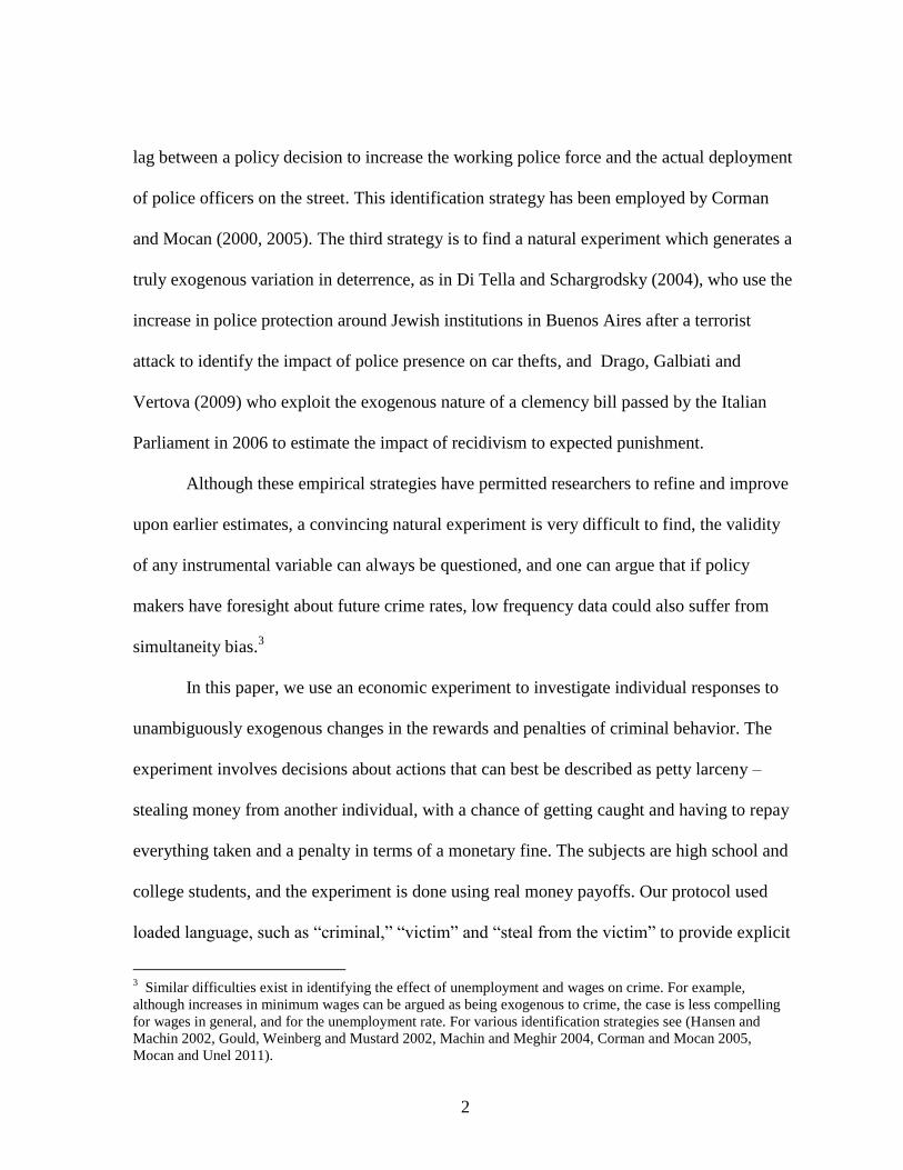
other is not supported, on average. Table 4 presents the distribution of the number of thefts.

During the experiment each individual had the opportunity to steal 13 times. Thus, zero thefts

means that the individual never stole during the experiment, while a 13 indicates that he or

she stole something in every choice set. As Table 4 demonstrates, there is substantial

variation in the number of thefts. Ten percent of the subjects stole five or fewer times. Forty-

seven percent of the subjects stole 13 times during the experiment; that is, they stole some

amount of money in very choice set.

We exploited the panel nature of the data and estimated the effects of loot,

probability, and fines on the decision to steal, as follows. Let Yi stand for the indicator

variable that takes the value of one if the individual decides to steal, and zero otherwise; and

let P stand for the vector that consists of the values of the loot, the probability of getting

caught, and the fine, associated with that choice. Assume that subject i has decided to steal in

a given choice set – for example, suppose she has decided to choose the last theft in choice

set 5, shown in Table 1. She has chosen a crime with loot of $8, a probability of being

caught of 75%, and a fine of $5.50 if caught. From her observed choice we can make the

revealed preference argument that this theft dominates the option not to steal, so Yi=1 with

8

these values of the loot, the probability of being caught, and the fine that are associated with

this crime P=($8, 75%, $5.50).6

A subject, who has decided not to steal from a given choice set, has made a series of

decisions not to steal, each relative to the option of stealing. So, again using choice set 5 as

an example, the choice with loot = $2, probability of being caught =75%, and fine =$0.10

was not enough for him to make the decision to steal. Thus, in this case, Yi=0, and P=($2,

75%, $0.10). The same is true for all other alternatives that involve stealing money in this

choice set, and so Y=0 for all other P vectors in choice set 5, given that the person did not

steal in that particular choice set.

Table 5 presents the results of the regressions using these data. In these and all other

regressions, standard errors are clustered at the individual level. The models behind columns

(1)-(3) include individual fixed-effects. An increase in the loot is expected to increase the

probability of committing theft. On the other hand, an increase in the probability of getting

caught and an increase in the fine should deter the individual from stealing. Column (1)

presents the results from the high school sample, and column (2) reports the results based on

the sample of college students. In both cases, an increase in the loot increases the propensity

to steal and an increase in fine decreases that propensity. The same is true for the probability

of getting caught, although the coefficient is insignificant in the college sample. When we

estimated the model by pooling high school and college students, and interacting the

explanatory variables with an indicator variable that identifies the high school students, we

could not reject the hypothesis that the coefficients were the same between the two groups.7

6 There could be another theft option in the same choice set that could have enticed the subject to steal (see the 7

theft options in Table 1), but given that the subject was allowed to make only one choice from each choice set,

we do not observe his second, or third-best theft choices. 7 The F-value of the joint significance of the interaction terms was1.21 with a p-value of 0.31.

9

Therefore, we estimated the model using the entire sample, which consists of 3,135

observations from 116 subjects. The results, reported in column (3) show that the point

estimates of the variables are almost identical to those reported in columns (1) and (2), and

that they are highly statistically significant.

The results in columns (1)-(3) of Table 5 indicate that a $1 increase in the amount of

money that is available to steal (loot) increases the probability of theft by 3 percentage

points. The mean value of the loot in the sample is $3.82, and the baseline theft propensity is

0.36. Thus, the elasticity of theft with respect to money available to steal is 0.32.

Important policy questions hinge on the relative deterrent effects of increased fines

versus increased chances of apprehension. Ideally, empirical studies would be done with data

that includes independent changes of both variables. However, in practice, empirical analyses

do not include measures of both the probability of apprehension and the severity of

punishment, because of the paucity of data. While it is possible to measure the probability of

apprehension by arrest rates of particular crimes, the severity of punishment is difficult to

quantify because data on conviction rates and average sentence lengths are noisy and they are

not consistently available. Therefore, crime regressions typically include arrests rates or the

size of the police force as measures of the certainty of punishment, with no controls for the

severity of punishment.8 9

8 One exception is research on the impact of capital punishment, where empirical models include measures of

the probability of arrest, the probability of conviction given arrest, and the probability of execution given

conviction (Mocan and Gittings 2010, Mocan and Gittings 2003, Ehrlich 1975). Mustard (2003) has personally

collected data on conviction rates and sentence lengths from four states and showed that the inability to include

these variables because of the lack of data under-states the impact of the arrest rate as much as 50 percent.

9 Over the last three decades the severity of punishment has been increased in many states in the U.S. with the

implementation of sentencing guidelines and mandatory sentencing policies. However, these sentencing reforms

are not exogenous events. Furthermore, they generate reactions in the behavior of judges and prosecutors,

which make certainty of punishment endogenous to these changes (Bushway, Owens and Piehl 2011, Miceli

2008, Schanzenbach and Tilelr, 2007).

10

Our design allows us to exogenously vary both the certainty and the severity of

punishment, and analyze the extent to which these variations induce a change in behavior.

We find strong evidence for deterrence effect. Furthermore, our results show that the

propensity to steal reacts more strongly to the penalty than to the probability of getting

caught. This result is consistent with the theoretical models where the potential offender is

risk averse (Ehrlich 1973). With the simplest specification, column (3) in Table 5, we find

that a one-percentage point increase in the probability of getting caught decreases the

propensity to steal by 0.3 percentage points, which corresponds to an elasticity of -0.4. This

elasticity is very similar to the elasticity of felony crimes with respect to their own arrest

rates reported by Corman and Mocan (2005) and in Levitt (1998). Similarly, if the fine goes

up by $1, we find the propensity to steal declines by about 5 percentage points, which

corresponds to a fine elasticity of theft of -0.30.

Column (4) of Table 5 presents the results from the linear probability model that

includes personal background characteristics of the individuals instead of individual fixed-

effects. Because data on these characteristics are collected only from high school students,

these regressions are restricted to the high school sample. Column (5) displays the marginal

effects obtained from a probit regression, and demonstrates that neither the point estimates

nor their statistical significance are altered by estimation methodology as the results are very

similar to those reported in column (4). The strong deterrence effect is confirmed in these

specifications as well. An increase in the probability of getting caught, or in the amount of

penalty reduces the incentive to steal as the estimated coefficients are highly significant in

columns (4) and (5).

11

The estimated impacts of personal attributes reveal interesting regularities. Males

have a higher propensity to steal than females, which has been well-documented in empirical

studies (Mocan and Rees 2005; Gottfredson and Hirshi 1990; Hagan, Simpson and Gillis

1979). The longer the individual has lived in the town where the experiments were

conducted, the lower his/her propensity to steal. Specifically, an additional year of residence

reduces the propensity to steal by about 2 percentage points. This result may be due to the

fact that longer residency is correlated with stronger personal networks, which in turn

reduces the propensity to steal - despite the fact that the victim is always anonymous. As

Levitt and List (2007) describe, utility maximization in situations like this may also involve

not only monetary payoffs, but also concerns about “doing the right thing” or “moral

choices.” In our setting, the declining propensity to steal as a function of the length of

residency in the city seems consistent with the hypothesis that difficult-to-observe

determinants of behavior such as “morals” may in part be determined by considerations of

the environment.10

The significance of the residency variable suggests that the subjects did

not treat the experiment as a game of chance - if they had, the length of residency would not

have any impact on their behavior.

Columns (4) and (5) also show that the age, the height and the GPA of the individual

have no impact on the propensity to steal.11

The same is true for the amount of money they

spend each week. Similarly, the endowment given to them in the beginning of the experiment

($8, $12 or $16) has no impact on the decision to steal. On the other hand, those who have

two or more siblings have a higher propensity to steal in comparison to those who have one

10

This is consistent with the results of Mocan (2011). 11

Adjusting for age, height could be a proxy of the uterine environment (including disease and

mother’s nutrition intake) and childhood nutrition and therefore a marker for cognitive ability (see

Case and Paxson 2008, Resnik 2002, and literature they cite).

12

sibling or no siblings. This result is in line with a large literature in economics, sociology and

demography which demonstrates the negative impact of family size on child outcomes

(Blake 1991, Becker and Lewis 1973, Downey 1995, Caceres-Delpiano 2006).12

In our final specifications we added an additional explanatory variable, the interaction

term between the probability of getting caught and the fine to the specifications. The

hypothesis is that the marginal effect of a given increase in the probability of getting caught

should be increasing in the fine, (or alternatively that the marginal impact of the fine should

be increasing in the probability of getting caught.) The results are reported in Table 6. As

before, all standard errors are clustered at the individual-level. Columns (1) and (2) report the

results of the models that employ the high school sample and the full sample, respectively.

The estimated coefficients are almost identical in both samples. As expected, the interaction

term between the probability of getting caught and fine is negative and statistically

significant. Using the estimates in column (2) we find that the impact on the propensity to

steal of a one-percentage point rise in the probability of getting caught, evaluated at the mean

value of fine ($2.12) is equal to -0.003 (0.001-0.002x2.12). This means, for instance, that a

five percentage point increase in the probability of detection lowers the propensity to steal by

1.5 percentage points if the amount of the fine is $2. If the penalty for stealing is $3, the same

five-percentage point increase in the probability of detection generates a decline in the

propensity to steal by 2.5 percentage points. A one dollar increase in the penalty reduces the

propensity to steal by 3.5 percentage points if the probability of getting caught is 40%.

However, if the probability of getting caught is 50%, the same one-dollar increase in fine

generates a decline in theft propensity by 5.5 percentage points.

12

In these specifications, the variable Oldest Child is coded as 1 if the person has no siblings. Alternatively,

assigning the value of zero to Oldest Child when the person is the only child had no impact on the results.

Excluding the Oldest Child variable did not change the results either.

13

Columns (3) and (4) of Table 6 report the estimation results of the model using the

high school sample and with the addition of personal characteristics of the individuals.

Column (3) displays the estimated coefficients from the linear probability model, and column

(4) shows the marginal effects obtained from probit. The entries in column (4) represent the

average marginal effect of the corresponding variable on the propensity to steal. The impact

of the interaction term is implicitly incorporated into the probability of getting caught and

into the fine variable when calculating the marginal effects.

Table 7A displays these impacts in a compact fashion. The Panel A of Table 7A

reports the marginal impact of the fine, obtained from both the linear probability

specification (column 3) and the probit specification (column 4) that employ the high school

sample, when the probability of getting caught ranges from 35% to 65%. An increase in the

certainty of punishment, represented by higher chances of getting caught, increases the

impact of the fine.

Panel B of the table reports the exercise from the other angle, and displays the

calculated impact of an increase in the certainty of punishment when the severity of

punishment gets bigger. The deterrent effect of the probability of getting caught gets bigger

as the severity of punishment (represented by the magnitude of the fine) gets larger.

Table 7B presents the results of the same exercise, but in this case, we use the entire

sample (high school student and college students). As in Table 7A, the results are based on

two specifications: the linear probability model reported in column 2 of Table 6, and the

corresponding probit model. The results are very similar to those displayed in Table 7A. The

impact of the penalty gets larger as the probability of detection is higher. Similarly, the

impact of the probability of detection gets larger as the penalty increases.

14

In order to investigate whether the results differ between the individuals who stole

more frequently and those who did not steal as frequently, we re-estimated the models using

only the individuals who stole six or fewer times during the experiment, and then using those

who stole 7-to-13 times. Table 8 presents the marginal effects obtained from both the linear

probability and the probit models in the sample of frequent stealers (those who decided to

steal more than six times during the experiment) as well as less-frequent stealers. The

marginal effects of the probability of getting caught and the fine are always negative. As

before, the impact of the certainty (severity) of punishment gets larger as the severity

(certainty) goes up. It is interesting to note that, although the marginal effects are somewhat

larger in the sample of those who stole more frequently, the elasticity of theft with respect to

fine and with respect to the probability of getting caught is larger in the sample of less-

frequent thefts. This is primarily because the baseline propensity to steal is lower in the group

of people who did not steal as frequently. This means that a given percentage-point decline in

the propensity to steal is translated into a larger percent change and therefore a larger

elasticity. For example, in Panel A of Table 8 we see that when the probability of getting

caught is 45%, the marginal effect of the fine is about -0.07 among those who stole more

than six times, and it is -0.03 among those who stole less than seven times. However, the

elasticity of theft with respect to fine is -0.28 in the former group, while it is -1.98 in the

latter group.

IV. Discussion and Conclusion

The extent to which criminals and potential criminals respond to variations in

deterrence is an important issue, both theoretically and from a public policy perspective.

15

Despite significant progress in recent empirical analyses in identifying the causal effect of

deterrence on crime, objections are still raised on the validity of methods proposed to

eliminate the simultaneity between crime and deterrence in empirical analyses, and some

social scientists continue to argue that criminal activity does not respond to sanctions. The

issue is important because it involves fundamental arguments about the rationality of

individuals in their decisions to engage in illegal acts and whether individuals respond to

changes in the costs of crime, such as the probability of punishment and the penalty they

face, if caught.

In this paper we analyze individuals’ responses to potential criminal opportunities

and the associated costs in an experimental setting. In our experiment subjects are exposed to

exogenous variations in the relative tradeoffs between three important aspects of criminal

opportunities – the amount of money they can steal from another person, the probability of

getting caught, and the penalty (fine) they pay if caught. We conducted the experiment with

juveniles and young adults, age groups that are near the peak ages for participation in petty

crime and who are frequently labeled as “irrational” and “unresponsive to deterrence.”

The instructions of the experiment employed loaded language, using the words

“criminal,” “victim,” “stealing,” “getting caught” repeatedly, to explicitly underline the

dishonest nature of the act. The experimental design always gave the option of not stealing.

We find that the propensity to steal responds to exogenous variations in the amount of money

available to steal, and in the certainty and severity of punishment. An increase in the

probability of getting caught reduces the propensity to steal, and the same is true for an

increase in the size of the penalty. The elasticity of theft with respect to the fine is bigger

than the elasticity with respect to the probability of getting caught. Furthermore, the impact

16

of the certainty of getting caught is larger when the penalty is bigger. Similarly, the deterrent

effect of the penalty is bigger when the probability of getting caught is bigger.

The caveats are that the “criminals” in these experiments are not necessarily

criminals outside the laboratory, and that the crimes do not involve very large financial gains

or losses, and because of the anonymity they do not involve social sanctions. Given these

qualifications, these results demonstrate that individuals’ decisions to commit crime are

consistent with the predictions obtained from economic models, in that exogenous changes in

enforcement and penalties do alter criminal behavior.

17

Table 1

Sample Bundles, from Choice Set # 5

Mark one choice

below

Amount to steal

from the victim

Chance of being

caught

Fine if you are

caught

$0.00 0% $0.00

$2.00 75% $0.10

$2.00 50% $2.10

$2.00 25% $4.10

$4.00 75% $1.90

$4.00 50% $3.90

$6.00 75% $3.70

$8.00 75% $5.50

18

Table 2

Choice Set Characteristics

Choice

Sets

Loot

(min, max)

Probability of

getting caught

(min, max)

Fine

(min, max)

1 $2.00, $8.00 25%, 75% $0.10, $5.70

2 $2.00, $8.00 25%, 75% $0.10, $2.90

3 $2.00, $8.00 25%, 75% $0.10, $5.70

4 $2.00, $8.00 25%, 75% $0.10, $2.90

5 $2.00, $8.00 25%, 75% $0.10, $5.50

6 $2.00, $8.00 25%, 75% $0.10, $2.80

7 $2.00, $8.00 25%, 75% $0.10, $5.50

8 $2.00, $8.00 25%, 75% $0.10, $2.80

9 $2.00, $6.00 25%, 75% $0.10, $4.10

10 $2.00, $6.00 25%, 75% $0.10, $2.10

11 $1.00, $6.00 55%, 55% $0.60, $0.60

12 $1.00, $6.00 55%, 55% $1.80, $1.80

13 $1.00, $6.00 5%, 5% $0.10, $0.10

In each of the 13 choice sets, there is one option with loot=$0.00, the probability of getting caught=0% ,

and fine=$0.0. This is the option of not stealing. Thus, the actual minimum values of the loot, the

probability of getting caught and the fine are 0.0 in each round. The values in the table pertain to the

minimum and maximum values among the choices that involve theft.

19

Table 3

Descriptive Statistics of Personal Characteristics

Variable Definition High

School Undergraduate

Age Age of the individual 16.86

(1.30) NA

Height Height of the individual in feet 5.60

(0.36) NA

GPA*

High school GPA if the

individual is in high school; the

average of high school and

college GPAs if the in college

3.46

(0.50) NA

Money How much money the individual

spends on his/her own per week

20.72

(28.36) NA

Male Dichotomous variable (=1) if the

person is male 0.41 NA

One Sibling*

Dichotomous variable (=1) if the

person has one sibling 0.47 NA

Two or more*

Siblings

Dichotomous variable (=1) if the

person has two or more siblings 0.46 NA

Oldest Child

Dichotomous variable (=1) if the

The person is the oldest child in

the family

0.48 NA

Years in

Eugene

The number of years the person

lived in Eugene, Oregon

9.75

(3.61) NA

N 82 34 * GPA information is missing for 3 students; sibling information is missing for 1

student. Socio-demographic data were not collected from the college sample.

20

Table 4

Number of Thefts

Number

of Thefts*

Number of

Individuals

Percentage of

Total

0 5 4.31%

1 1 0.86%

2 1 0.86%

3 1 0.86%

4 1 0.86%

5 3 2.59%

6 2 1.72%

7 4 3.45%

8 2 1.72%

9 8 6.90%

10 9 7.76%

11 5 4.31%

12 19 16.38%

13 55 47.41%

Total 116 100%

*The number of thefts is the number of choice sets

where the individual stole money. Thus, 0 indicates

that the individual did not steal money during the entire

experiment, and 13 indicates that he/she stole in every

choice set.

21

Table 5

The Impact of Rewards and Sanctions on the Propensity to Steal

Variable (1) (2) (3) (4) (5)

Loot 0.033*** 0.040*** 0.034*** 0.051*** 0.046***

(0.006) (0.013) (0.006) (0.008) (0.008)

Probability of -0.003*** -0.002** -0.003*** -0.005*** -0.004***

getting caught (0.001) (0.001) (0.000) (0.001) (0.001)

Fine -0.058*** -0.043*** -0.055*** -0.072*** -0.068***

(0.010) (0.015) (0.008) (0.011) (0.011)

Age 0.013 0.012

(0.031) (0.029)

Male 0.383*** 0.342***

(0.088) (0.074)

Height -0.201 -0.173

(0.143) (0.129)

GPA 0.053 0.050

(0.080) (0.078)

Endowment -0.006 -0.005

(0.010) (0.009)

Money 0.001 0.001

(0.002) (0.002)

Years in Eugene -0.018* -0.015*

(0.009) (0.009)

One Sibling 0.063 0.077

(0.144) (0.147)

Two or more

siblings

0.294*

(0.149)

0.290**

(0.146)

Oldest child -0.007 0.005

(0.072) (0.070)

Sample High

school College Pooled Pooled Pooled

Individual FE Yes Yes Yes No No

R-squared 0.09 0.12 0.10 0.22 0.18#

N 2,509 626 3,135 2,368 2,368 Standard errors, reported in parentheses, are clustered at the individual level. Statistical

significance of the coefficients at the 10%, 5% and 1% level are indicated by *, **, and ***.

Models in columns (1)-(4) are estimated by OLS. Column (5) reports the average marginal

effects obtained from maximum likelihood probit. # represents pseudo-R square.

22

Table 6

The Impact of Rewards and on the Propensity to Steal (with interaction)

Variable (1) (2) (3) (4)

Loot 0.065*** 0.067*** 0.099*** 0.090***

(0.009) (0.009) (0.011) (0.010)

Probability of 0.0003 0.001 0.0001 -0.007***

Getting caught (0.0009) (0.001) (0.001) (0.001)

Fine 0.038** 0.045*** 0.073*** -0.097***

(0.017) (0.015) (0.021) (0.012)

Probability x -0.002*** -0.002*** -0.003***

Fine (0.0003) (0.0003) (0.0005)

Age 0.0121 0.011

(0.029) (0.028)

Male 0.364*** 0.322***

(0.085) (0.070)

Height -0.189 -0.156

(0.137) (0.123)

GPA 0.050 0.048

(0.078) (0.076)

Endowment -0.005 -0.004

(0.009) (0.009)

Money 0.001 0.001

(0.002) (0.002)

Years in Eugene -0.017* -0.014*

(0.009) (0.008)

One Sibling 0.059 0.069

(0.143) (0.143)

Two or more

siblings

0.277*

(0.148)

0.269*

(0.143)

Oldest child -0.008 0.003

(0.069) (0.068)

Sample

High School

Pooled High School

High School

Individual FE Yes Yes No No

R-squared 0.14 0.20 0.25 0.25#

N 2,509 3,402 2,368 2,368 Standard errors, reported in parentheses, are clustered at the individual level. Statistical

significance of the coefficients at the 10%, 5% and 1% level are indicated by *, **, and

***. Models in columns (1)-(3) are estimated by OLS. Column (4) reports the average

marginal effects obtained from maximum likelihood probit. The estimated probit model

includes an interaction term for (probability of getting caught) x (fine). The reported

marginal effects of the probability of getting caught and the fine implicitly include the

impact of the interaction term. # represents the pseudo-R square value.

23

Table 7A

The Effect of Certainty and Severity of Punishment

(High School Sample)

Panel A

Linear Probability Model

Probability of Getting Caught 35% 45% 55% 65%

-0.039***

(0.010)

-0.071***

(0.010)

-0.103***

(0.012)

-0.135***

(0.015)

Probit

Probability of Getting Caught 35% 45% 55% 65%

-0.039***

(0.011)

-0.071***

(0.010)

-0.096***

(0.010)

-0.113***

(0.011)

Panel B

Linear Probability Model

Fine $1 $1.5 $2 $2.5 $3

-0.003***

(0.001)

-0.005***

(0.001)

-0.006***

(0.001)

-0.008***

(0.001)

-0.009***

(0.001)

Probit

Fine $1 $1.5 $2 $2.5 $3

-0.003***

(0.001)

-0.005***

(0.001)

-0.006***

(0.001)

-0.007***

(0.001)

-0.008***

(0.001)

The entries are the changes in the probability of stealing as fine goes up by $1, or as the probability of

getting caught goes up by 1 percentage point based on models in columns (3) and (4) of Table 6. The

standard errors are calculated using the Delta method.

24

Table 7B

The Effect of Certainty and Severity of Punishment

(Pooled Sample)

Panel A

Linear Probability Model

Probability of Getting Caught 35% 45% 55% 65%

-0.032***

(0.007)

-0.054***

(0.008)

-0.076***

(0.009)

-0.098***

(0.011)

Probit

Probability of Getting Caught 35% 45% 55% 65%

-0.028**

(0.009)

-0.068***

(0.009)

-0.103***

(0.009)

-0.128***

(0.010)

Panel B

Linear Probability Model

Fine $1 $1.5 $2 $2.5 $3

-0.002***

(0.001)

-0.003***

(0.001)

-0.004***

(0.001)

-0.005***

(0.001)

-0.006***

(0.001)

Probit

Fine $1 $1.5 $2 $2.5 $3

-0.003***

(0.001)

-0.005***

(0.001)

-0.006***

(0.001)

-0.008***

(0.001)

-0.009***

(0.001)

The entries are the changes in the probability of stealing as fine goes up by $1, or as the probability of

getting caught goes up by 1 percentage point. The specification is the one reported in column (2) of Table

6, and it is estimated by both OLS and probit. Standard errors are calculated using the Delta method.

25

Table 8

The Effect of Certainty and Severity of Punishment by Frequency of Stealing

(Pooled Sample)

Panel A

Frequent Theft (>6)

Linear Probability Model

Probability of Getting Caught

35% 45% 55% 65%

-0.034***

(0.010)

-0.065***

(0.009)

-0.096***

(0.010)

-0.128***

(0.012)

Probit

-0.034**

(0.012)

-0.078***

(0.011)

-0.121***

(0.009)

-0.156***

(0.007)

Less Frequent Theft (<7)

Linear Probability Model

Probability of Getting Caught

35% 45% 55% 65%

-0.021**

(0.010)

-0.026***

(0.010)

-0.031***

(0.010)

-0.037***

(0.011)

Probit

-0.024**

(0.011)

-0.031***

(0.011)

-0.031***

(0.011)

-0.028***

(0.011)

Panel B

Frequent Theft (>6)

Linear Probability Model

Fine

$1 $1.5 $2 $2.5 $3

-0.001

(0.001)

-0.003***

(0.001)

-0.004***

(0.001)

-0.006***

(0.001)

-0.007***

(0.001)

Probit

-0.002**

(0.001)

-0.004***

(0.001)

-0.006***

(0.001)

-0.009***

(0.001)

-0.011***

(0.001)

Less Frequent Theft (<7)

Linear Probability Model

Fine

$1 $1.5 $2 $2.5 $3

-0.002***

(0.001)

-0.002***

(0.001)

-0.003***

(0.001)

-0.003***

(0.001)

-0.003***

(0.001)

Probit

-0.002***

(0.001)

-0.002***

(0.001)

-0.002***

(0.001)

-0.002***

(0.001)

-0.002***

(0.001) The entries are the changes in the probability of stealing as fine goes up by $1, or as the probability of

getting caught goes up by 1 percentage point. The specification is the one reported in column (2) of Table

6, and it is estimated by both OLS and probit. Standard errors are calculated using the Delta method.

26

Appendix – Protocol

Welcome:

Today we are conducting an experiment about decision-making. Your decisions are for real

money, so pay careful attention to these instructions. This money comes from a research

foundation. How much you earn will depend on the decisions that you make, the decisions of

others, and on chance.

Secrecy:

All your decisions will be secret and we will never reveal them to anyone. We will ask you to

mark your decisions on paper forms using a pen or pencil. If you are discovered looking at

another person’s forms, or showing your form to another person, we cannot use your decisions in

our study and so you will not get paid. Please do not talk during the experiment.

Payment:

You have been given a packet. Stapled to this packet is a card with a number on it. This is your

claim check number. Each participant has a different number. Please tear off your card now. Be

sure that your claim check number is written on top of the first page of your packet, but do not

turn the page until instructed to do so. Be sure to keep your claim check number. You will

present this number to an assistant in exchange for your payment envelope.

The Experiment:

You are going to play a game today. In this game you will be randomly and anonymously paired

with another person in the room. One of you will be the criminal, and the other will be the

victim. You will not know who you are paired with, even after the game is over.

Each person will start with some money, but the amount of money each person gets may be

different. You will start with either $16, $12, or $8. Your starting endowment has been

determined randomly. The amount you start with is recorded on your packet.

The criminal will have a chance to steal some of the victim’s money. However, stealing is not

without a risk. If the criminal decides to steal some of the victim’s money, there is a chance that

the criminal is caught. If the criminal is caught, then he or she will have to return the money

taken from the victim, and also pay a fine to the experimenter. The chance that the criminal is

caught, and the amount of the fine, depend on the choice made by the criminal.

Everyone received one packet, and each packet contains 13 different sheets stapled together. We

will show you an example. We call these Choice Sheets.

On each Choice Sheet everyone will make a choice as if you are the criminal. You will declare

your choice of how much money to steal from the victim by putting a check mark next to one of

the choices.

27

When we play the game the amount of money you will end up with will really be determined by

the choices you make, so you want to consider your choice very carefully. We will give you 60

seconds on the first page and 30 seconds on each subsequent page. Please leave your pen on the

desk and do not mark your choice until I ask you to do so. When the time is up I will ask you to

place a check mark next to the choice you want. It is important that you wait until the time is up

to mark your choice.

After everyone has made a choice on each of the 13 Choice Sheets, you will have a chance to

reconsider each of your decisions just to make sure you have considered each choice carefully. If

you wish to change your decision, please cross out your old decision and mark your new

decision with a red pen. We will give you 30 seconds on the first page and 15 seconds on each

subsequent page. Please leave your pen on the desk and do not mark your choice until I ask you

to do so. When the time is up I will ask you to place a check mark next to the choice you want. It

is important that you wait until the time is up to mark your choice.

Next we have to determine who will be the criminal and who will be the victim. We randomly

assign roles by flipping a coin. If it comes up heads, then those whose claim check number is

even will be assigned the role of the criminal, and those whose claim check number is odd will

be assigned the role of the victim. Should the coin come up tails, then those whose claim check

number is odd will be assigned the role of the criminal, and those whose claim check number is

even will be assigned the role of the victim.

Now we have to pick which one of the 13 Choice Sheets will count. We will pick a random

number from 1 to 13, by having your teacher draw a card from a deck of 13 cards. The Ace will

stand for 1, the Jack, Queen, and King will stand for 11, 12, and 13 respectively. The number of

the card will determine which Choice Sheet counts. We will have you turn your packet to that

choice sheet.

Note that you don’t know which of your 13 decisions will count before you make all of your

decisions, if any. This will be determined purely by chance. So, the best thing for you to do is to

treat every choice sheet as if it will count, and make the choice on that sheet that you most

prefer.

In the final step of the game we have to determine whether or not the criminal is caught. Here is

how this will work: We have 4 index cards. On each index card there is a percentage written.

They are: 25%, 50%, 75% and 100%. We will randomly choose one of these index cards.

Everybody looks at their choice on the Choice Sheet that has just been selected. If you are the

criminal, and if the percentage written on the selected index card is less than or equal to the

chance of being caught for the choice you made on the Choice Sheet, then you are caught. You

will have to return the money you stole from the victim and pay the corresponding fine to the

experimenter. Otherwise you keep the money.

Now we will collect your decision packets and calculate your payments. To calculate your

payments, we will randomly match one criminal with one victim. To get your envelope, we will

ask you to fill out a receipt to be returned to us.

28

References

Alm, J., G. H. McClelland and W. D. Schulze. (1992) "Why Do People Pay Taxes?," Journal of

Public Economics, 48, 21-38.

Alm, J. and M. McKee. (2006) "Audit Certainty, Audit Productivity, and Taxpayer

Compliance," National Tax Journal, 59, 801-816.

Alm, J. and M. McKee. (2004) "Tax Compliance as a Coordination Game," Journal of

Economic Behavior and Organization, 54 3, 297-312.

Becker, Gary S. (1968) “Crime and punishment: an economic approach,” Journal of Political

Economy, 76, 169-217.

Becker, Gary and H. Gregg Lewis (1973). "On the Interaction between the Quantity and Quality

of Children". The Journal of Political Economy, 81, 279–288

Blake, Judith. (1981) “Family size and the quality of children,” Demography, 18(4), 421-442.

Block, M. and M. Heineke. (1975) “A labor theoretic analysis of the criminal choice,” American

Economic Review, 65, 314-325.

Bushway, Shawn D., Emily G. Owens and Anne Morrison Piehl (2011) “Sentencing Guidelines

and Judicial Discretion: Quasi-experimental Evidence from Human Calculation Errors,”

NBER Working Paper, No. 16961

Cáceres-Delpiano, Julio. (2006) “The Impacts of Family Size on Investment in Child Quality,”

Journal of Human Resources, XLI(4), 738-754.

Case, Anne and Christina Paxson. (2008), "Stature and status: Height, ability, and labor market

outcomes," Journal of Political Economy, 116(3), 499-532.

Corman, H. and Naci Mocan. (2000) “A time-series analysis of crime, deterrence and drug

abuse in New York City,” American Economic Review, 90, 584-604.

_____. (2005) “Carrots, sticks, and broken windows,” Journal of Law and Economics, 48, 235-

266.

Di Tella, R. and E. Schargrodsky. (2004) “Do police reduce crime? Estimates using the

allocation of police forces after a terrorist attack,” American Economic Review, 94, 115-

134.

Downey, Douglas B. (1995) “When Bigger Is Not Better: Family Size, Parental Resources, and

Children's Educational Performance,” American Sociological Review, 60(5), 746-761.

29

Drago, Francesco, Roberto Galbiati and Pietro Vertova. (2009), "The Deterrent Effects of Prison:

Evidence from a Natural Experiment," The Journal of Political Economy, 117(2), 257-

280

Ehrlich, I. (1973) “Participation in illegitimate activities: a theoretical and empirical

investigation,” Journal of Political Economy, 81, 521-565.

_____. (1975). “The deterrent effect of capital punishment: a question of life and death,”

American Economic Review, 65, 397-417.

_____. (1996). “Crime, Punishment, and the Market for Offenses,” Journal of Economic

Perspectives, 10:1, 43-67.

Flinn, C. (1986) “Dynamic models of criminal careers.” In Blumstein, A. et al. (eds.), Criminal

Careers and “Career Criminals”. Washington DC: National Academy Press.

Gottfredson, Michael R. and Travis Hirschi, (1990), "A General Theory of Crime," Stanford

University Press

Gould, Eric, Bruce Weinberg and David Mustard (2002), “Crime Rates and Local Labor Market

Opportunities in the United States: 1979-1997,” Review of Economics and Statistics, 84,

pp.45-61.

Hansen. Kirstine and Stephen Machin (2002), “Spatial Crime patterns and the Introduction of the

UK Minimum Wage,” 64, Oxford Bulletin of Economics and Statistics, pp. 677-697.

Hagan, J., John H. Simpson, and A.R. Gillis. (1979). "The sexual stratification of social control:

A gender-based perspective on crime and delinquency," British Journal of Sociology,

30(1), 25-38.

Layson, S. K. (1985) “Homicide and deterrence: a reexamination of the United States time-

series evidence,” Southern Economic Journal, 52, 68-89.

Levitt, S. D. (2002) “Using electoral cycles in police hiring to estimate the effect of police on

crime: reply,” American Economic Review, 92, 1244-1250.

Levitt Steven D. and John A. List (2007) “What Do Laboratory Experiments Tell Us About the

Real World?” Journal of Economic Perspectives, 21(2), pp.153-74.

Levitt, Steven D. (1998) "Why Do Increased Arrest Rates Appear to Reduce Crime: Deterrence,

Incapacitation, or Measurement Error?" Economic Inquiry, 36, 353-372.

Machin, Stephen and Costas Meghir (2004) “Crime and Economic Incentives,” Journal of

Human Resources, 39 (4), pp. 958-79.

30

Miceli, Thomas J. (2008) “Criminal Sentencing Guidelines And Judicial Discretion,”

Contemporary Economic Policy, 26(2), 207-215.

Mocan, Naci H. (2011), "Vengeance." Revised version of the NBER Working Paper No: 14131.

Mocan, H. Naci and Kaj Gittings. (2010), "The Impact of Incentives on Human Behavior: Can

We Make It Disappear? The Case of the Death Penalty," in The Economics of Crime:

Lessons For & From Latin America; Rafael DiTella, Sebastian Edwards and Ernesto

Schargrodsky (eds.), Chicago: University of Chicago Press, 2010; pp. 379-418.

Mocan, H. Naci and Kaj Gittings. (2003) “Getting Off Death Row: Commuted Sentences and the

Deterrent Effect of Capital Punishment,” Journal of Law and Economics, 46(2), 453-478.

Mocan, Naci, Steve Billups and Jody Overland. (2005) "A Dynamic Model of Differential

Human Capital and Criminal Activity," Economica, 72, 655-81.

Mocan, Naci H. and Daniel Rees. (2005) “Economic Conditions, Deterrence and Juvenile Crime:

Evidence from Micro Data,” American Law and Economics Review. 7(2), 319-349.

Mocan, Naci and Bulent Unel. (2011) "Skill-Biased Technological Change, Earnings of Low-

skill Workers, and Crime," Working Paper.

Mustard, David B. (2003) "Reexamining Criminal Behavior: The Importance of Omitted

Variable Bias," The Review of Economics and Statistics, 85(1), 205-211.

Resnik, Robert. (2002) “Intrauterine Growth Restriction.” Obstetrics and Gynecology, 99, 490–

496.

Schanzenbach, Max M. and Emerson H. Tiller. (2007) “Strategic Judging Under the United

States Sentencing Guidelines: Positive Political Theory and Evidence,” The Journal of

Law, Economics, and Organization, 23, 24–56.

Schmidt, Peter and Ann Dryden Witte. (1984) An Economic Analysis of Crime and Justice:

Theory, Methods, and Evidence. Academic Press.

Witte, A. D. (1980) “Estimating Economic Models for Crime With Individual Data,” Quarterly

Journal of Economics, 94, 57-84.