The Zonal Dipole Pattern of Tropical Cyclone Genesis in the Indian Ocean Influencedby the Tropical Indo-Pacific Ocean Sea Surface Temperature Anomalies

JUNPENG YUAN

Key Laboratory of Atmospheric Environment and Processes in the Boundary Layer over the Low-Latitude Plateau Region,

Department of Atmospheric Sciences, Yunnan University, Kunming, China

YONG GAO

Key Laboratory of Atmospheric Environment and Processes in the Boundary Layer over the Low-Latitude Plateau

Region, Department of Atmospheric Sciences, Yunnan University, Kunming, and Meteorological Bureau of

Tibet Autonomous Region, Lhasa, China

DIAN FENG AND YALI YANG

Key Laboratory of Atmospheric Environment and Processes in the Boundary Layer over the Low-Latitude

Plateau Region, Department of Atmospheric Sciences, Yunnan University, Kunming, China

(Manuscript received 16 January 2019, in final form 24 June 2019)

ABSTRACT

From a basinwide perspective, the dominant mode of Indian Ocean tropical cyclone genesis (TCG) in

September–November (SON) shows an equatorially symmetric east–west zonal dipole pattern, which can

explain approximately 13% of the SON TCG variance. This zonal dipole TCG pattern is significantly related

to the tripole pattern of the sea surface temperature anomalies (SSTAs) in the tropical Indo-Pacific Ocean

(IPT). The IPT, which is a combined interbasin mode and presents a dipole pattern of SSTAs in the tropical

IndianOcean andElNiño–like SSTAs in the tropical PacificOcean, can influence the localWalker circulation

and zonal dipole TCGpattern over the tropical IndianOcean.Associated with a positive IPT phase, abnormal

ascending (descending)motions are induced and favorable formore (less) water vapor transport to the lower–

middle level in the western (eastern) tropical Indian Ocean; significant anticyclonic vorticity anomalies are

evoked in the lower level over the eastern tropical Indian Ocean, and weak easterly vertical wind shear

appears over the tropical IndianOcean. Thus, abnormally strong upwardmotion, abundant water vapor in the

lower–middle level, and weak vertical wind shear are favorable for more TCG in the western tropical Indian

Ocean, while the combined negative contributions of the vertical motion, lower-level vorticity, and humidity

terms result in less TCG in the eastern tropical Indian Ocean.

1. Introduction

Tropical cyclones (TCs) are among the most destructive

weather systems in the world and span the global tropical

oceans. The Indian Ocean is one of the oceans prone to

TCs. In the northern Indian Ocean, including the Bay

of Bengal (BOB) and Arabian Sea (AS), TCs exhibit a

unique bimodal seasonal distribution caused by unfa-

vorable environmental conditions during the monsoon

season (Li et al. 2013). Peak TC activity occurs during

September–November, with a secondary maximum dur-

ing April–June (Fig. 1a). In the southern Indian Ocean,

TC genesis (TCG) gradually increases in the season of

September–November (SON) and reaches the peak sea-

son in December–March (Fig. 1b).

The primary source of energy for TCs is the heat

transferred from ocean to atmosphere; thus, the local

sea thermal states are very important to TC activities

(Gray 1968; Rotunno and Emanuel 1987). The Indian

Ocean dipole (IOD) mode, of which the sea surface

temperature anomalies (SSTAs) vary oppositely be-

tween the western and southeastern tropical Indian

Ocean, is a distinct mode in the Indian Ocean on in-

terannual time scales (Saji et al. 1999; Webster et al.

1999). Although the SSTAs are asymmetric about the

equator in the eastern Indian Ocean during IOD events,Corresponding author: Junpeng Yuan, jpyuan@ynu.edu.cn

1 OCTOBER 2019 YUAN ET AL . 6533

DOI: 10.1175/JCLI-D-19-0042.1

� 2019 American Meteorological Society. For information regarding reuse of this content and general copyright information, consult the AMS CopyrightPolicy (www.ametsoc.org/PUBSReuseLicenses).

Unauthenticated | Downloaded 12/20/21 01:03 AM UTC

the induced wind curl anomalies are quite symmetric

about the equator (Li et al. 2003; Schott et al. 2009). By

modifying the local thermal states and large-scale at-

mospheric circulation, the IOD may exert a great in-

fluence on TC activities in both the southern and

northern IndianOcean (Singh 2008; Yuan andCao 2013;

Li et al. 2015; Li et al. 2016). Results of Yuan and Cao

(2013) indicate that TC activities in the northern Indian

Ocean are closely related to IOD events; that is, fewer

(more) TCs occur in the BOB and AS regions during

positive (negative) IOD years. Singh (2008) found a sig-

nificant negative correlation between the September–

October IOD index and the BOB TC frequency in

November and suggested that, with a lead time of one

month, the IOD could be a potential predictor of intense

cyclones in November over the BOB. By compositing the

monthly TC frequencies in positive and negative IOD

years, Li et al. (2015, 2016) observed that TC frequencies

over both the BOB and the southeastern Indian Ocean

exhibit significant differences during October–November

between positive and negative IOD years.

As a dominant interannual mode in the tropical

oceans, El Niño–Southern Oscillation (ENSO) may also

exert a remote influence on the genesis, frequency,

track, and intensity of TCs over the Indian Ocean,

through induced large-scale atmospheric circulation

(e.g., Ho et al. 2006; Girishkumar and Ravichandran

2012; Ng and Chan 2012; Felton et al. 2013; Sumesh and

Kumar 2013). Compared with El Niño, La Niña condi-

tions offer a more favorable environment for TC activity

over the BOB (Ng and Chan 2012; Felton et al. 2013;

Mahala et al. 2015), especially in October–December

(Girishkumar and Ravichandran 2012; Felton et al.

2013). In addition, Girishkumar et al. (2015) indicated

that the ENSO–TC relationship in October–December

over the BOB can be modified by the Pacific decadal

oscillation, with a more significant relationship in warm

Pacific decadal oscillation phases. Balaguru et al. (2016)

also showed that ENSO induces a meridional dipole

mode of TC activity in the BOB during the premonsoon

season of May–June through a modulation of the mon-

soon circulation. ENSO can also modify TC activity in

the southern Indian Ocean (Ho et al. 2006;Werner et al.

2012); more (fewer) TCs occur in the southwestern

tropical Indian Ocean during El Niño (La Niña) years(Kuleshov et al. 2008; Ash and Matyas 2012).

Previous works have revealed that TC activities in

several regions of the Indian Ocean, such as the BOB

and the southwestern and southeastern Indian Ocean,

may be influenced by both the local SSTAs in the

tropical Indian Ocean and remote SSTAs in the tropical

Pacific Ocean. However, these studies focused mainly

on the influences of the IOD/ENSO on TC activities in

one single sea region of the Indian Ocean. It should be

noted that the IOD/ENSO-induced oceanic processes

and atmospheric circulation anomalies are significant

and widespread in both the northern and southern

tropical Indian Oceans. However, the influences of the

tropical Indo-Pacific Ocean SSTAs on the TC activities

in the whole Indian Ocean on a basinwide scale are

as yet unclear. Moreover, there remain some uncer-

tainties over the extent of the IOD/ENSO link to the

Indian Ocean TC activities. For example, the BOB TCs

are found to be more active in the co-occurrences of

La Niña and negative IOD years (Girishkumar and

Ravichandran 2012; Mahala et al. 2015). However,

composite analysis has shown that the differences of

BOB TCG in October–November are significant be-

tween the positive and negative IOD years, but not

significant between El Niño and La Niña years (Li et al.2015). Also, in the southern Indian Ocean, Li et al.

(2016) observed that the TC frequency in October–

November is co-affected by El Niño and positive IOD

events, but La Niña seems to have limited influence. Liu

and Chan (2012) investigated the ENSO/IOD link to the

TC activities in the southern Indo-Pacific Ocean, and

suggested that ENSO and the IOD cannot be treated as

separate modes. The atmospheric circulation anoma-

lies induced by ENSO and the IOD are difficult to

separate completely, especially on an interannual time

scale (Saji et al. 1999; Yuan and Li 2008; Xie et al. 2009;

FIG. 1. Monthly frequency distribution of TCG in the

(a) northern and (b) southern IndianOcean during 1981–2015. The

red box highlights the season of SON on which this study focuses.

6534 JOURNAL OF CL IMATE VOLUME 32

Unauthenticated | Downloaded 12/20/21 01:03 AM UTC

Girishkumar and Ravichandran 2012). Thus, it is nec-

essary to take the tropical Indo-Pacific Ocean as a whole

to investigate its influence on the TCs in the Indian

Ocean. This work mainly focuses on the basinwide scale

TCG in the Indian Ocean and investigates the rela-

tionship between the Indian Ocean TCG and the SSTAs

of the entire tropical Indo-Pacific Ocean.

As shown in Fig. 1, TCG in the north Indian Ocean

exhibits a bimodal seasonal distribution, comprising

54.4% and 29.4% of the total TCG during the peak

season of September–November and the secondary

maximum during April–June, respectively, whereas in

the southern Indian Ocean approximately 7.4% and

6.3% of the total TCG occurs during September–

November and April–June, respectively. For the dif-

ferences of the seasonal distribution of TCG and

background circulations in the northern and southern

Indian Ocean, we focus on the season of SON, which is

the peak season of TCG in the northern Indian Ocean

and the season that TCs begin to be more active in the

southern Indian Ocean. SON is also a season of strong

atmosphere–ocean interactions in the Indo-Pacific

Ocean (Ju et al. 2004; Chen 2011; Lian et al. 2014),

when the signals induced by both ENSO and the IOD

are strong (Chen 2011; Lian et al. 2014) and may exert

great influence on TCG in the Indian Ocean.

This paper is organized as follows: section 2 describes

the dataset andmethods used for the study. An overview

of TCG over the Indian Ocean during 1981–2015 is

presented in section 3. Section 4 shows the relationship

between the TCG in the Indian Ocean and SSTAs in

the tropical Indo-Pacific Ocean. Section 5 investigates

the impact of tropical Indo-Pacific Ocean SSTAs on the

TCG environments in the Indian Ocean. A summary of

our findings is presented in section 6.

2. Data and methods

a. Datasets

The TC datasets during 1981–2015 are extracted from

the Joint Typhoon Warning Center over the northern

and southern Indian Ocean (Chu et al. 2002).The pres-

ent study focuses exclusively on TCs with the maximum

sustainedwind speeds greater than 34kt (17ms21); thus,

only tropical storms and typhoons are considered.

The following datasets for the period 1981–2015 are

also used: monthly atmospheric data at 0.758 3 0.758resolution from the European Centre for Medium-

Range Weather Forecasts interim reanalysis (ERA-

Interim; Dee et al. 2011), and monthly SST on a 28 3 28grid from version 3b of the Extended Reconstructed

SST dataset of the National Oceanic and Atmospheric

Administration (Smith et al. 2008).

b. The IOD mode index and Niño-3.4 index

Following Saji et al. (1999), the Indian Ocean dipole

mode index (DMI) is defined as the differences of the

averaged SON SSTAs between the western (108S–108N,

508–708E) and eastern (108S–08, 908–1108E) tropical In-dianOcean. For ENSO, the averaged SONSSTAs in the

Niño-3.4 region (58N–58S, 1708–1208W) are computed to

represent theNiño-3.4 index. For ease of comparison, all

variables are standardized by first subtracting the mean

from the raw data, and then dividing the difference by

the standard deviation. All discussion on the various

time series is therefore based on standardized values,

unless otherwise stated.

c. TC genesis potential index

Climatologically, cyclone genesis is intimately re-

lated to large-scale environmental factors, including

low-level relative vorticity, Coriolis forcing, vertical

shear of the horizontal winds, the sea surface thermal

state, conditional instability through a deep atmo-

spheric layer, and humidity in the lower and middle

troposphere (Gray 1968, 1979). Motivated by the work

of Gray (1979), Emanuel and Nolan (2004) developed

the TC genesis potential index (GPI) to describe

quantitatively the influences of large-scale environ-

mental factors on cyclone genesis. Murakami and

Wang (2010) further redefined the GPI by explicitly

incorporating the vertical motion term to improve the

reproducibility of TCG over regions with strong as-

cending motions. Recently, Wang and Moon (2017)

indicated that the vertical motion is a meaningful fac-

tor for TCG in the Indian Ocean. Thus, the present

study uses the GPI developed by Murakami and Wang

(2010) to determine the factors responsible for TCG

location changes in the tropical Indian Ocean. The

formulation of the GPI is as follows:

GPI

5 j105hj3/2�RH

50

�3 Vpot

70

� �3(11 0:1V

shear)22

�2v1 0:1

0:1

�,

(1)

where h is the absolute vorticity (s21) at 850 hPa, RH

is the relative humidity (%) at 700 hPa, Vpot is the

maximum potential intensity (m s21), Vshear is the

magnitude of the vertical zonal wind shear (m s21)

between 200 and 850 hPa, and v is the vertical pres-

sure velocity (omega; Pa s21) at 500 hPa. The defini-

tion of maximum potential intensity is based on

Emanuel (1995), and was modified by Bister and

Emanuel (1998). A FORTRAN source code for com-

puting the maximum potential intensity is available

1 OCTOBER 2019 YUAN ET AL . 6535

Unauthenticated | Downloaded 12/20/21 01:03 AM UTC

online (ftp://texmex.mit.edu/pub/emanuel/TCMAX/pcmin_

revised.f).

To assess quantitatively the individual contributions

of each term in Eq. (1) to the total GPI, the GPI change

is decomposed using the method of Li et al. (2013) and

Li et al. (2016). The following introduction of the

method is derived from Li et al. (2016) with minor

modifications. First a natural logarithm is taken on both

sides of the GPI formula, and then a total differential is

applied to both sides; thus the change of GPI can be

separated into five terms, as below:

dGPI5a13 dTerm11a

23 dTerm21a

3

3 dTerm31a43 dTerm41a

53 dTerm5, (2)

where

8>>>>>>><>>>>>>>:

a15Term23Term33Term43Term5

a25Term13Term33Term43Term5

a35Term13Term23Term43Term5

a45Term13Term23Term33Term5

a55Term13Term23Term33Term4.

This method shows some skill in the diagnosis of the

relative contribution of environmental factors to TCG in

both the northern and southern Indian Ocean (Li et al.

2013; Li et al. 2015; Li et al. 2016). The present work also

applies this GPI quantitative method to assess the con-

tribution of each large-scale factor to TCG.

d. Moisture budget diagnosis

The moisture tendency equation at a constant pressure

level is used to analyze specific processes that cause the

specific humidity anomaly (Yanai et al. 1973; Hsu and Li

2012; Li et al. 2013; Li et al. 2016). The tendency equation

for the specific humidity anomaly q0 is written as

›q0

›t52(V=q)0 2

�v›q

›p

�02

�Q

2

L

�0, (3)

where q is the specific humidity,V is the horizontal wind

vector, 2(V=q)0 indicates anomalous horizontal mois-

ture advection, p is the pressure, v is the vertical pres-

sure velocity, 2[v(›q/›p)]0 denotes anomalous vertical

moisture advection, Q2 is the atmospheric apparent

moisture sink, and L is the latent heat of condensation.

In addition, empirical orthogonal function (EOF)

analysis is used to reveal the spatiotemporal character-

istics of TCG in the Indian Ocean. Singular value de-

composition (SVD) analysis is carried out to verify the

relationship between the TCG in the Indian Ocean and

SSTAs in the tropical Indo-Pacific Ocean.

Correlation, regression, and composite analysis are

also used in this paper. North’s significance test (North

et al. 1982) is used for significance testing of the EOF

and SVD analysis. The two-sided Student’s t test, which

gives the probability that the means for two groups are

statistically different at the 90% and 95% confidence

levels, is used for significance testing of the compos-

ite analysis. Monthly anomalies of all quantities here

are computed by removing the climatological monthly

means.

3. Overview of TCG in the Indian Ocean

During the period 1981–2015, there were a total of 92

and 67 TCs generated in the northern and southern In-

dian Ocean in SON, respectively. In the northern Indian

Ocean, most of the TCs are generated in the BOB and

eastern AS. TCs form frequently in the regions of 608–1008E around 108S in the southern Indian Ocean

(Fig. 2a). The frequency of TCG was also counted in

each 58 3 58 box in the Indian Ocean, which measures

how frequently TCs are formed within a specific grid

FIG. 2. (a) Geographical distribution of TCG number (shaded) in each 58 3 58 grid box during 1981–2015. (b) The

distribution of GPI (shaded) during 1981–2015. The dots indicate TCG locations.

6536 JOURNAL OF CL IMATE VOLUME 32

Unauthenticated | Downloaded 12/20/21 01:03 AM UTC

box. Thus, we can use the TCG number in each box to

investigate the spatiotemporal variations of TCG in the

Indian Ocean.

EOF analysis is used to reveal the spatiotemporal

characteristics of the TCG frequency in the Indian

Ocean. The dominant first mode of EOF analysis

(EOF1) of TCG shows a zonal dipole variation pattern

in both the northern and southern Indian Ocean

(Fig. 3a). The frequency of TCG varies oppositely in

the east and west parts of the Indian Ocean, with high

positive (negative) loadings centered in the AS and

southwestern Indian Ocean (BOB and southeastern

Indian Ocean). This indicates that TCG in the north-

ern and southern Indian Ocean covaries as an equa-

torially symmetric east–west zonal dipole pattern. The

EOF1 mode explains approximately 13% of the SON

TCG variance. Note that 13% is not a very big per-

centage of TCG variance, and may be partly owing to

the differences of the TCG seasonal distributions in

the northern and southern Indian Ocean (Fig. 1). The

North’s significance test for the TCG EOF analysis

indicates that the EOF1 mode is a clearly independent

mode. The time series of the EOF1 mode shows ap-

parent interannual variation (Fig. 3b), with fewer

(more) TCG events in the BOB and southeastern In-

dian Ocean and more (fewer) in the AS and south-

western Indian Ocean during the positive (negative)

anomaly years (Fig. 3a). Wavelet analysis indicates

that the EOF1 mode varies mainly at a quasi-5-yr scale

(figure not shown).

4. Relationship between the Indian Ocean TCGand tropical Indo-Pacific SSTAs

The relationships of TCG in the Indian Ocean with

the SSTAs of the tropical Indo-Pacific Ocean are in-

vestigated in this section. The correlations between the

time series of the TCG EOF1 mode and the SSTAs in

the tropical Indo-Pacific Ocean show a distinct tripole

pattern (Fig. 4a). Significant positive correlations appear

in the western tropical IndianOcean and central-eastern

equatorial Pacific Ocean, but negative correlations are

present in the Maritime Continent regions. It appears

that the zonal dipole pattern of TCG in the Indian

Ocean is significantly connected with the combined ef-

fects of the SSTAs in both the tropical Indian and Pacific

Oceans. In Fig. 4a, the distribution of the correlation

coefficient features an IOD-like pattern in the tropical

Indian Ocean and El Niño–like pattern in the tropical

Pacific Ocean. The correlation coefficients of the TCG

EOF1 time series with DMI and Niño-3.4 indices are

0.45 and 0.35, and significant at the 99% and 95%

FIG. 3. First empirical orthogonal function (EOF1)mode of SON

TCG frequency in the Indian Ocean during 1981–2015: (a) spatial

distribution and (b) standard time series.

FIG. 4. (a) Correlation coefficients (shaded) of the time series of

the Indian Ocean TCGEOF1mode and SSTAs in the Indo-Pacific

Ocean during 1981–2015. The black plus signs or dots indicate that

the correlation coefficient passes the significance test at the 95% or

90% confidence level, respectively. Also shown are the leading

EOF1modes of the SON SSTAs in the tropical Indo-Pacific Ocean

during 1981–2015: (b) spatial distribution and (c) standard time

series (the blue bar). The red line in (c) shows the IPT index.

1 OCTOBER 2019 YUAN ET AL . 6537

Unauthenticated | Downloaded 12/20/21 01:03 AM UTC

confidence levels, respectively. To note that, numerous

works have revealed that intimate connections exist be-

tween the IOD and ENSO (e.g., Webster et al. 1999; Li

et al. 2003; Xie et al. 2009). The correlation coefficient of

DMI and Niño-3.4 is 0.63, which is very high and signifi-

cant at the 99% confidence level. After removing the

Niño-3.4-regressed simultaneous signals, the correlation

coefficient of the TCG EOF1 and DMI is decreased to

0.29, but also significant at the 90% confidence level.

These imply that the TCGEOF1modemay relate to both

ENSO and the IOD. However, ENSO and the IOD are

closely linked, and it is hard to separate their individual

effects completely, especially on an interannual time scale.

Moreover, only focusing on a single basin mode of the

IOD/ENSO also may not accurately reflect the individual

effects. Thus, it is necessary to take the SSTAs of the

tropical Indo-Pacific Ocean as a whole to investigate their

combined influences on the TCG in the Indian Ocean.

Note that the signals in the eastern tropical PacificOcean

are very strong while the SSTAs in the Indian Ocean are

relatively weak (Ju et al. 2004; Xie et al. 2009). But the

west–east zonal gradient of SSTAs in the IndianOceanmay

also be very important to TCG. To investigate the com-

bined impacts of the SSTAs in the tropical Indo-Pacific

Ocean, we chose the western tropical Indian Ocean, Mar-

itime Continent region, and the equatorial central-eastern

Pacific Ocean, shown as three boxes with significant cor-

relation coefficients in Fig. 4a, as the key regions to define

an Indo-Pacific tripole (IPT) index for describing the tripole

pattern of SSTAs in the tropical Indo-Pacific Ocean. The

detailed formula of the IPT index is as follows:

IPT5SST12 SST

21 SST

3, (4)

whereSST1,SST2, andSST3 are the averaged SON SSTAs

of the western tropical Indian Ocean (108S–108N, 508–708E), the Maritime Continent region (108S–08, 908–1408E), and the central-eastern equatorial Pacific Ocean

(58S–58N, 1708–908W), respectively. Previous studies have

indicated that the tropical Indian and Pacific Oceans are

closely connected through the Walker circulation and In-

donesian Throughflow (Xie et al. 2009; Chen 2011; Lian

et al. 2014; Huang et al. 2016; Li et al. 2018). Alongside the

Walker circulation anomalies over the tropical Indo-Pacific

Ocean, opposite west–east gradients of sea surface tem-

perature appear in the tropical Indian and Pacific Oceans,

and the interbasin scale SSTAs of the tropical Indo-Pacific

Ocean present as an obvious IPT pattern (Ju et al. 2004;

Chen and Cane 2008; Chen 2011; Lian et al. 2014). EOF

analysis of the averaged SON SSTAs in the tropical Indo-

Pacific Ocean (208S–208N, 408E–908W) during 1981–2015

shows that the dominant EOF1 mode is a similar tripole

pattern and can explains approximately 63% of the total

SSTA variances (Fig. 4b). This EOF1 mode presents as an

IOD-like pattern in the tropical Indian Ocean and an El

Niño–like pattern in the tropical Pacific Ocean, which is

consistent with the results in previous studies (Ju et al.

2004; Chen 2011; Liu et al. 2019). The time series of the

tropical Indo-Pacific SSTA EOF1 mode relates highly to

the IPT index (Fig. 4c), and the correlation coefficient is

0.97. This indicates that the IPT pattern is a distinct com-

bined mode of SSTAs in the tropical Indian and Pacific

Oceans. Previous studies have revealed that the IPTmode

can reflect the covariation/coexistence of the SSTAs of

ENSO in the tropical Pacific Ocean and the IOD in the

tropical IndianOcean (Lian et al. 2014; Liu et al. 2019). By

investigating the tropical Indo-Pacific Ocean SSTAmodes

on the TCG variation over the western North Pacific, Liu

et al. (2019) found that the combined IPT mode can ex-

plain larger TCG variation than the individual SSTA

modes in the tropical Indian and Pacific Oceans. This

confirms our motivation to investigate the combined im-

pacts of the IPT mode on the TCG in the Indian Ocean.

The TCG EOF1 mode is closely related to the IPT

with a correlation coefficient of 0.45 and is significant at

the 99% confidence level. Further analysis showed that 20

of a total of 35 years are at a TCGEOF1positive phase, of

which 65% of the years are in co-occurrence with IPT

positive years (13 years); meanwhile, 15 years are at a

TCG EOF1 negative phase, 87% of which are in co-

occurrencewith IPT negative phases (Table 1). To further

validate the relationships between the IndianOceanTCG

EOF1 mode and the IPT pattern in the tropical Indo-

Pacific Ocean, we chose the IPT positive (negative) phase

years that are in co-occurrence with TCG EOF1 posi-

tive (negative) phase years as the typical IPT positive

TABLE 1. List of the years at positive/negative phases of the TCG_EOF1 and IPTmodes. The boldface type indicates the 13 positive years

and 13 negative years that are described as ‘‘typical’’ in the text.

Positive years Negative years

TCG_EOF1 1981, 1982, 1986, 1989, 1990, 1993, 1994,

1997, 2002, 2003, 2004, 2006, 2009, 2011,

2012, 2013, 2014, and 2015

1983, 1984, 1985, 1987, 1988, 1991, 1992,

1995, 1996, 2000, 2001, 2005, 2007,

2008, and 2010

IPT 1982, 1986, 1987, 1991, 1993, 1994, 1997,2002, 2003, 2004, 2006, 2009, 2012,

2014, and 2015

1981, 1983, 1984, 1985, 1988, 1989, 1990,1992, 1995, 1996, 2000, 2001, 2005, 2007,

2008, 2010, 2011, and 2013

6538 JOURNAL OF CL IMATE VOLUME 32

Unauthenticated | Downloaded 12/20/21 01:03 AM UTC

(negative) years. The 13 typical IPT positive years and 13

typical IPT negative years are presented in Table 1.

In typical IPT positive years, the SSTAs feature a tri-

pole pattern in the tropical Indo-Pacific Ocean, with sig-

nificant positive anomalies in the western tropical Indian

Ocean and the central-eastern equatorial Pacific Ocean,

but negative anomalies in the southeastern tropical

IndianOcean andwestern tropical PacificOcean (Fig. 5a).

Correspondingly, most TCs are generated in the west part

of the Indian Ocean. Especially in the southern Indian

Ocean, approximately 95% (18 out of a total of 19) of

TCG is located west of 858E. However, in typical IPT

negative years, the composite SSTAs also present as a

tripole pattern in the tropical Indo-Pacific Ocean, but al-

most opposite to that in IPT positive years (Fig. 5b). TCs

mainly are generated in the east part of the Indian Ocean.

FIG. 5. Composite of the SON averaged SSTAs (contours; 8C) in the (a) typical positive IPT

years and (b) typical negative IPT years. (c) The differences of TCG number between the

typical positive and negative IPT years (shaded). The shaded parts in (a) and (b) indicate that

the composited SSTAs pass the significance t test at the 95% confidence level. The red dots in

(a) and (b) indicate TCG locations. A black plus sign or dot in (c) indicates that the differences

of TCG number pass the significance test at the 95% or 90% confidence level, respectively.

1 OCTOBER 2019 YUAN ET AL . 6539

Unauthenticated | Downloaded 12/20/21 01:03 AM UTC

In this composite, 82% (28 of a total of 34) of the north

Indian Ocean TCG is in the BOB, and all TCs are formed

east of 708E in the south Indian Ocean. The differences of

TCG between the typical positive and negative IPT years

show that significant negative TCG anomalies appear in

the southeastern Indian Ocean and BOB, while positive

TCG anomalies appear in the southwestern Indian Ocean

and AS (Fig. 5c). The above-mentioned correlation and

composite analysis indicate that the zonal dipole pattern of

TCG in the Indian Ocean is significantly related to the

tropical Indo-Pacific tripole SSTA pattern.

We also carried out an SVD analysis of the IndianOcean

TCGfrequency and tropical Indo-PacificOceanSSTAs and

obtained an analogous coupledmode (figure not shown). In

the SVD coupled mode, the SST field presents a distinct

tripole variation pattern in the Indo-Pacific Ocean, and its

correlation coefficientwith the IPT is 0.9,which is significant

at the 99% confidence level; meanwhile, the Indian Ocean

TCG field shows a zonal dipole pattern with high positive

loadings centered in the BOB and southeastern Indian

Ocean, and its correlation with the TCG EOF1 mode is

0.79, which is also significant at the 99% confidence level.

The coupledmode is the firstmode of the SVDanalysis and

occupies 72% of the coupled variance contributions, which

can explain ;62% of SSTAs of the tropical Indo-Pacific

Ocean and ;9% of TCG variations in the Indian Ocean.

The SVD coupled mode reflects the relationship between

the TCG EOF1 mode and IPT. According to the North’s

significance test, this SVD coupled mode is a clear and in-

dependent mode. These confirm that the zonal dipole TCG

mode in the Indian Ocean is closely related to the IPT

pattern of SSTAs in the tropical Indo-Pacific Ocean with

certainty. More (fewer) TCs formed in the west (east) part

of both the northern and southern Indian Ocean at IPT

positive phases; the opposite is true at IPT negative phases.

5. Modulation of Indian Ocean TCG environmentsby the tropical Indo-Pacific SSTAs

a. Climatic environments of the IndianOcean in SON

In SON, the warm sea surface temperature encom-

passed by the 268C isothermal lines can be found

north of 158S in the southern Indian Ocean, the BOB,

and the AS in the northern Indian Ocean (Fig. 6a).

FIG. 6. The SON averaged (a) sea surface temperature (8C), (b) 850-hPa wind (vectors; m s21) and vorticity

(shaded; 1025 s21), (c) vertical zonal wind shear between 200 and 850 hPa (shaded; m s21) and 700-hPa specific

humidity (contours; 1022 kg kg21), and (d) 500-hPa omega (1022 Pa s21) during 1981–2015.

6540 JOURNAL OF CL IMATE VOLUME 32

Unauthenticated | Downloaded 12/20/21 01:03 AM UTC

Accompanying the easterly (westerly) wind in the south

(north) of the equatorial Indian Ocean at 850 hPa, a pair

of cyclonic wind curls appear around 58–158 in the

southern and northern regions of the tropical Indian

Ocean. Strong cyclonic vorticities present in the tropical

southern Indian Ocean, western AS, and BOB regions

(Fig. 6b). The relative humidity shows a similar distri-

bution pattern to the sea surface temperature field, with

high values east of 608E of the tropical Indian Ocean

(Fig. 6c). The regions of weak vertical wind shear are

located within a zonal strip 58–158 on both sides of the

Indian Ocean (Fig. 6c). Strong ascending motions

mainly appear east of 608E in the southern IndianOcean

and BOB regions (Fig. 6d).

b. Favorable conditions for the zonal dipole patternof TCG in the Indian Ocean

To investigate the favorable conditions for the zonal

dipole pattern of TCG in the Indian Ocean, we used the

time series of TCG EOF1 mode to regress the oceanic

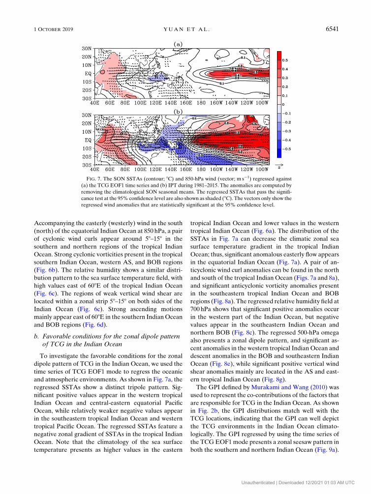
and atmospheric environments. As shown in Fig. 7a, the

regressed SSTAs show a distinct tripole pattern. Sig-

nificant positive values appear in the western tropical

Indian Ocean and central-eastern equatorial Pacific

Ocean, while relatively weaker negative values appear

in the southeastern tropical Indian Ocean and western

tropical Pacific Ocean. The regressed SSTAs feature a

negative zonal gradient of SSTAs in the tropical Indian

Ocean. Note that the climatology of the sea surface

temperature presents as higher values in the eastern

tropical Indian Ocean and lower values in the western

tropical Indian Ocean (Fig. 6a). The distribution of the

SSTAs in Fig. 7a can decrease the climatic zonal sea

surface temperature gradient in the tropical Indian

Ocean; thus, significant anomalous easterly flow appears

in the equatorial Indian Ocean (Fig. 7a). A pair of an-

ticyclonic wind curl anomalies can be found in the north

and south of the tropical Indian Ocean (Figs. 7a and 8a),

and significant anticyclonic vorticity anomalies present

in the southeastern tropical Indian Ocean and BOB

regions (Fig. 8a). The regressed relative humidity field at

700 hPa shows that significant positive anomalies occur

in the western part of the Indian Ocean, but negative

values appear in the southeastern Indian Ocean and

northern BOB (Fig. 8c). The regressed 500-hPa omega

also presents a zonal dipole pattern, and significant as-

cent anomalies in the western tropical IndianOcean and

descent anomalies in the BOB and southeastern Indian

Ocean (Fig. 8e), while significant positive vertical wind

shear anomalies mainly are located in the AS and east-

ern tropical Indian Ocean (Fig. 8g).

The GPI defined by Murakami and Wang (2010) was

used to represent the co-contributions of the factors that

are responsible for TCG in the Indian Ocean. As shown

in Fig. 2b, the GPI distributions match well with the

TCG locations, indicating that the GPI can well depict

the TCG environments in the Indian Ocean climato-

logically. The GPI regressed by using the time series of

the TCGEOF1mode presents a zonal seesaw pattern in

both the southern and northern Indian Ocean (Fig. 9a).

FIG. 7. The SON SSTAs (contour; 8C) and 850-hPa wind (vector; m s21) regressed against

(a) the TCG EOF1 time series and (b) IPT during 1981–2015. The anomalies are computed by

removing the climatological SON seasonal means. The regressed SSTAs that pass the signifi-

cance test at the 95% confidence level are also shown as shaded (8C). The vectors only show the

regressed wind anomalies that are statistically significant at the 95% confidence level.

1 OCTOBER 2019 YUAN ET AL . 6541

Unauthenticated | Downloaded 12/20/21 01:03 AM UTC

FIG. 8. As in Fig. 7, but for (a),(b) 850-hPa wind (vectors; m s21) and vorticity (shaded; 1026 s21);

(c),(d) 700-hPa relative humidity (shaded; 1022 kg kg21); (e),(f) 500-hPa omega (shaded; 1022 Pa s21)

and precipitation (only negative values are shown in contours; mmday21); and (g),(h) vertical zonal wind

shear (m s21), regressed against the (left) TCG EOF1 time series or (right) IPT. In (a) and (b), the

regressed vorticity passing the significance test at the 95%confidence level is shaded, and thick blackwind

vectors indicate the regressedwinds that are statistically significant at the 95%confidence level. The black

dots in (c) and (d) denote the regressed relative humidity passing the significance test at the 95% con-

fidence level. The black dots in (e) and (f) denote the regressed omega passing the significance test at the

95% confidence level. The black dots in (g) and (h) denote the regressed wind shear passing the sig-

nificance test at the 95% confidence level.

6542 JOURNAL OF CL IMATE VOLUME 32

Unauthenticated | Downloaded 12/20/21 01:03 AM UTC

Significant positive GPI anomalies appear in the south-

western tropical Indian Ocean and AS, but negative

values present in the southeastern tropical IndianOcean

and northern BOB, indicating that the conditions fa-

vorable for TCG also present as a zonal dipole pattern.

Following Li et al. (2013), we applied the GPI quan-

titative method to assess the relative contribution of

each large-scale factor on TCG. The GPI terms are av-

eraged in four regions, with the AS region defined as

608–808E and 58–208N, the BOB region defined as 908–1008E and 58–208N, the southwestern Indian Ocean

(SWIO) region defined as 608–808E and 158–58S, and the

southeastern Indian Ocean (SEIO) region defined as

808–1008E and 158–58S.As shown in Fig. 10a, the relative contributions of the

vorticity term are negative in all four regions, indicating

that the low-level anticyclonic wind curls (Fig. 8a) are

unfavorable for TCG in both the west and east parts of the

tropical Indian Ocean. Especially in the BOB, the vor-

ticity term exerts the largest negative contribution to GPI.

Both the humidity and vertical motion terms show posi-

tive contributions in the AS and southwestern Indian

Ocean, but negative contributions in the BOB and

southeastern Indian Ocean. The moisture budget analysis

by using the moisture tendency equation shows that the

increase of special humidity at 700hPa in the AS and

southwestern Indian Ocean is primarily attributed to the

vertical motion transportation term, while the apparent

moisture sink has a negative contribution (Fig. 11a).

However, in the east part of the tropical IndianOcean, the

tendencies of special humidity anomaly are negative,

primarily because of negative contributions of the vertical

motion transportation term in the BOB and southeastern

Indian Ocean (Fig. 11a). Thus, the humidity anomaly

tendency at 700hPa is closely related to the vertical mo-

tion transportation term. Alongside significant anoma-

lous ascending (descending) motion in the AS and

southwestern Indian Ocean (BOB and southeastern In-

dian Ocean) (Fig. 8e), more (less) water vapor is trans-

ported upward to the lower–middle troposphere, which is

favorable (unfavorable) for deepening the moist layer

and causingmore (less) TCG in the western (eastern) part

of the tropical Indian Ocean. It appears that the west–east

seesaw distributions of the humidity and vertical mo-

tion terms are important to the zonal dipole pattern of

TCG in the Indian Ocean. The co-contributions of the

humidity and vertical motion terms to the total GPI in all

of the four regions are more than 50%, and show positive

(negative) contributions in the west (east) part of the

tropical Indian Ocean (Fig. 10a). The contributions of the

maximum potential intensity (PI) terms are relatively

weak in the Indian Ocean. The vertical wind shear term

presents positive contributions in all the four regions, es-

pecially with strong positive contributions in BOB andAS

regions. This is because the westerly wind shear anomalies

(Fig. 8g) can reduce the climatic easterly wind shear

(Fig. 6c); thus, it is favorable for TCG in the whole Indian

Ocean basin.

It appears that the west–east seesaw distributions of the

lower–middle-level humidity and vertical motion anom-

alies are important to the zonal dipole pattern of TCG in

the Indian Ocean. In the western part of the tropical In-

dian Ocean, the positive contributions of the humidity

and vertical motion terms combined with the vertical

wind shear term can overcome the negative effects of the

low-level vorticity term, which is favorable for more

TCG, while the combined negative contributions of the

humidity, verticalmotion, and vorticity terms result in less

TCG in the eastern part of the tropical Indian Ocean.

c. Modulation of Indian Ocean TCG environmentsby the tropical Indo-Pacific SSTAs

To investigate the modulation of TCG environments

by the tropical Indo-Pacific SSTAs, we also use the IPT

FIG. 9. As in Fig. 7, but for the GPI. Black dots denote the regressed GPI passing the significance test at the 95%

confidence level.

1 OCTOBER 2019 YUAN ET AL . 6543

Unauthenticated | Downloaded 12/20/21 01:03 AM UTC

index to regress the large-scale factors of TCG environ-

ments. Accompanying the IPT index variations, the

SSTAs in the tropical Indo-Pacific Ocean features signifi-

cant positive anomalies that appear in the western tropical

Indian Ocean and central-eastern equatorial Pacific

Ocean, but negative values appear in the Maritime Con-

tinent regions (Fig. 7b). The tripole SSTAs pattern can

leads to negative (positive) zonal gradients of sea surface

temperature and significant lower-level easterly (westerly)

wind anomalies in the tropical Indian (Pacific) Ocean

(Fig. 7b). The low-level easterly wind anomalies in the

tropical Indian Ocean and the westerly wind anomalies in

the tropical Pacific Ocean further cause obvious lower-

level divergence and force significant descending motion

anomalies in theMaritime Continent regions (Figs. 7b and

8f). Previous works have indicated that the Walker circu-

lations overlying the tropical Indian and Pacific Oceans

operate like two coupled gears, and are closely connected

by the common vertical motion branch over the Maritime

Continent regions (Wu and Meng 1998; Meng and Wu

2000). Therefore, the anomalous descending motion over

the Maritime Continent regions also can trigger the

Walker circulation anomalies over both the tropical Indian

and Pacific Oceans (Fig. 12b).

FIG. 10. The contributions of each of the GPI terms that are regressed against the (a) TCGEOF1 time series and

(b) IPT. TheAS region is defined as 608–808Eand 58–208N, theBOB region is defined as 908–1008E and 58–208N, the

SWIO region is defined as 608–808E and 158–58S, and the SEIO region is defined as 808–1008E and 158–58S.

FIG. 11. As in Fig. 10, but for the contributions of each term of the moisture tendency equation at 700 hPa

(1028 kg kg21 s21).

6544 JOURNAL OF CL IMATE VOLUME 32

Unauthenticated | Downloaded 12/20/21 01:03 AM UTC

Associated with the SSTAs of IPT, an obvious local

Walker circulation anomaly can be found over the trop-

ical Indian Ocean. Significant ascending (descending)

motion anomalies appear over the western (eastern)

tropical Indian Ocean, easterly wind anomalies appear in

the lower troposphere, and westerly wind anomalies ap-

pear in the upper troposphere over the tropical Indian

Ocean (Fig. 12b). The local Walker circulation anomaly

can significantly modify the TCG environments in the

entire tropical Indian Ocean basin. The possible physical

processes and interpretations are analyzed below.

First, the anomaly of the vertical branch of the local

Walker circulation can influence the upward moisture

transportation. The moisture budget analysis shows that

the vertical motion transportation term is primarily at-

tributed to the negative humidity anomalies tendency at

700hPa in the eastern part of the tropical Indian Ocean.

In the southwestern Indian Ocean, the vertical motion

transportation term exerts the largest contribution to

the positive tendency of the humidity anomalies. And

in the AS region, the combined positive contributions of

the vertical motion transportation term and horizontal

moisture advection term can overcome the negative

effect of the apparent moisture sink and result in a

positive humidity anomalies tendency (Fig. 11b). Thus,

it appears that the humidity anomaly tendency distri-

bution pattern of positive in the west and negative in the

east in the tropical Indian Ocean is closely related to the

vertical motion transportation term. The anomalous

ascending (descending) vertical motion can transport

more (less) water vapor to the lower–middle tropo-

sphere and is favorable (unfavorable) for TCG in the

western (eastern) part of the tropical IndianOcean. GPI

contribution analysis also shows that the changes of the

humidity term contribute greatly to the TCG variation,

especially for acting as the largest negative term con-

tribute to the TCG reductions in the BOB and south-

eastern tropical Indian Ocean (Fig. 10b).

Second, the descending motion anomalies in the east-

ern part of the tropical Indian Ocean are unfavorable for

FIG. 12. The vertical sections of velocity averaged in 108S–108N regions, which are regressed against the (a) TCG

EOF1 time series, (b) IPT, (c) DMI, and (d) Niño-3.4 index. Shading denotes the omega (1022 Pa s21). Vectors

denote that the regressed velocity passes the significance test at the 95% confidence level.

1 OCTOBER 2019 YUAN ET AL . 6545

Unauthenticated | Downloaded 12/20/21 01:03 AM UTC

convection, and lead to negative precipitation anomalies

in the BOB and southeastern tropical Indian Ocean

(Fig. 8f). As a Rossby wave response to the suppressed

precipitation and related atmospheric heat sink, a pair of

significant anticyclonic wind curl anomalies can be found

in the lower atmosphere of the tropical Indian Ocean

(Fig. 8b). These anticyclonic wind anomalies can signifi-

cantly reduce the lower troposphere cyclonic vorticity

and are unfavorable for TCG in the eastern part of the

tropical Indian Ocean (Figs. 8b and 9b). The vorticity

term is the second largest negative term contributing to

the TCG reductions in both the BOB and southeastern

tropical Indian Ocean (Fig. 10b).

Third, the Walker circulation anomalies can also

modify the zonal wind shear between the upper and

lower levels. The induced westerly wind anomalies in

the upper level and easterly wind anomalies in the lower

level can result in significant westerly wind shear over

the entire tropical Indian Ocean basin (Fig. 8h). It

should be noted that the climatology of the vertical wind

shear over the tropical Indian Ocean in SON is easterly

wind shear (Fig. 6c). Thus, the westerly wind shear can

reduce the climatic vertical wind shear and exert a

positive contribution to the GPI variation over the

whole tropical Indian Ocean (Fig. 10b). Quantitative

GPI analysis shows that the vertical shear term is im-

portant to the total of GPI variance in the western part

of the tropical Indian Ocean, which acts as the largest

(second largest) positive contribution term in the AS

(southwestern tropical Indian Ocean). Note also that in

the BOB region, although the vertical shear term shows

great positive contribution to the GPI variance, the

combined negative effects of the vorticity, humidity, and

vertical motion terms can overcome the positive con-

tribution of the vertical shear term, and result in TC

reduction. In contrast, the contribution of the vertical

shear term to TCG is relatively small in the southeastern

tropical Indian Ocean (Fig. 10b).

The Indian Ocean TCG is significantly affected by the

combined tripole pattern of SSTAs in the tropical Indian

and Pacific Oceans. The regressed Indo-Pacific Ocean

SSTAs and the above atmospheric environments related

to the IPT index exhibits very similar figures to those

regressed by the TCG EOF1 mode (Figs. 7 and 8). The

IPT pattern is related to the zonal dipole pattern of TCG

in the Indian Ocean, by modifying the local Walker

circulation and TCG environments. Associated with a

positive phase of IPT, abnormal ascending (descending)

motions are induced and favorable for more (less) water

vapor transport to the lower–middle level in the western

(eastern) tropical Indian Ocean; significant anticyclonic

wind anomalies are evoked in the lower level in the

eastern part of the tropical Indian Ocean, and weak

easterly vertical wind shear appears over the tropical

Indian Ocean. Thus, abnormally strong upward motion,

abundant water vapor, and weak vertical wind shear are

favorable for more TCG in the western part of the

tropical Indian Ocean, while the combined negative

contributions of the vertical motion, low-level vorticity,

and humidity terms result in less TCG in the eastern part

of the tropical Indian Ocean.

d. Possible links of the IOD/ENSO with the IPT andIndian Ocean TCG zonal dipole pattern

Numerous studies have revealed that intimate con-

nections exist in the air–sea interactions between the

tropical Indian and Pacific oceans (e.g., Wu and Meng

1998; Klein et al. 1999; Li et al. 2003; Meyers et al. 2007;

Chen and Cane 2008; Xie et al. 2009). The dominant

mode of the SSTAs in the tropical Indian and Pacific

Oceans is characterized as an obvious interbasin IPT

pattern (Ju et al. 2004; Chen 2011; Lian et al. 2014; Li

et al. 2018; Liu et al. 2019), which features IOD-like

SSTAs in the tropical Indian Ocean and El Niño–likeSSTAs in the tropical Pacific Ocean (Fig. 4b). The cor-

relation coefficients of the IPT with the DMI and Niño-3.4 indices are 0.8 and 0.94, respectively. Recently, the

IPT mode is widely treated as an interbasin mode and

combines the signals of both the IOD and ENSO (Lian

et al. 2014; Li et al. 2018; Liu et al. 2019).

Further analysis indicated that both of the DMI and

Niño-3.4 indices have significant correlations with the

TCG EOF1 mode, with the correlation coefficients of

0.45 and 0.35 and are significant at the 99% and 95%

confidence levels, respectively. The atmospheric circu-

lation anomalies regressed by the DMI and Niño-3.4indices also present similar configures as those regressed

by the IPT and the TCG EOF1 mode (Fig. 12). Obvious

Walker circulations anomalies appear overlying the

tropical Indian and Pacific Oceans, which operate like

two coupled gears and are closely connected by the

common vertical motion branch over the Maritime

Continent regions, consistent with the present studies

(e.g., Wu and Meng 1998; Meng and Wu 2000; Ju et al.

2004; Lian et al. 2014). Through this kind of atmospheric

bridge, ENSO signals over the Pacific Ocean and the

IOD impacts over the Indian Ocean are closely con-

nected, and may exert combined effects on the dipole

pattern of TCG in the Indian Ocean through modifying

the local Walker circulation anomalies.

To quantitatively depict the differences of TCG be-

tween the western and eastern parts of the tropical In-

dian Ocean, a TCG_Dipole index is defined as the

difference of the averaged SON TCG number between

thewestern (408–808E, 208S–208N) and eastern (908–1008E,208S–208N) tropical Indian Ocean. The TCG_Dipole

6546 JOURNAL OF CL IMATE VOLUME 32

Unauthenticated | Downloaded 12/20/21 01:03 AM UTC

index is highly related to the time series of the TCG

EOF1 mode, with the correlation coefficient of 0.62.

Thus, the TCG_Dipole index can quantitatively repre-

sent the variations of the zonal dipole pattern of TCG.

To further determine the possible links between the

IPT, ENSO, IOD, and Indian Ocean TCG dipole pat-

tern, we established multiple linear regression equa-

tions of TCG_Dipole variation on the combined DMI

and Niño-3.4 indices [Eq. (5)], and the SSTAs of three

key regions which are used to compute the IPT index

[Eq. (6)], respectively.

As shown in Eq. (5),

TCG_Dipole5 0:5753DMI1 0:5653Niño3:4, (5)

TCG_Dipole significantly relates to both the DMI and

the Niño-3.4 indices, with the correlation coefficients

of 0.575 and 0.565, respectively. The regressed TCG_

Dipole is significantly correlated with the raw dataset of

TCG_Dipole; its correlation coefficient is 0.63 and sig-

nificant at the 99% confidence level. The combined

contributions of the DMI and Niño-3.4 indices to TCG_

Dipole variance are approximately 39%, while the in-

dividual contributions of the DMI and Niño-3.4 indices

are 33% and 32%, respectively. These indicate that both

the DMI and Niño-3.4 indices relate to the zonal dipole

pattern of TCG in the Indian Ocean, but note that the

IOD and ENSO are not independent, with a high cor-

relation coefficient of 0.63.

Equation (6) shows the multiple linear regression

analysis of TCG_Dipole on the IPT index:

TCG_Dipole5 0:5863 SST12 0:482

3 SST21 0:5503 SST

3. (6)

By using the IPT index, the correlation coefficient be-

tween the raw TCG_Dipole and the regressed TCG_

Dipole is increased from 0.63 (with results from

the combined IOD/ENSO regression model) to 0.69

(with results from the IPT regression model), and the

contribution of the IPT index to the TCG_Dipole vari-

ance is improved to approximately 48%. These imply

that considering the interbasin IPT mode of the tropical

Indo-Pacific Ocean as a whole and using the IPT index

may be better for explaining the variances of the TCG

zonal dipole pattern in the Indian Ocean. On the one

hand, the Indian Ocean TCG dipole pattern is appears

to accompany the coupled gear-like operating Walker

circulation anomalies over both the tropical Indian and

Pacific Oceans (Fig. 12a). And the IPT mode can rep-

resents the combined interbasin SSTAs of both the

tropical Indian and Pacific Oceans, and has a better re-

lationship with the TCG dipole pattern in the Indian

Ocean. On the other hand, the IOD and ENSO events

are closely connected by complex atmospheric and

oceanic processes (e.g., Li et al. 2003; Xie et al. 2009; Ha

et al. 2017). It is hard to separate the individual effect of

the IOD/ENSO on the TCG variances in the Indian

Ocean. And it is also difficult to determine the linear

combination of the IOD/ENSO effect, especially when

the IOD and ENSO events have opposite effects on

the TCG.

6. Summary

From a basinwide perspective, the dominant mode of

the Indian Ocean TCG in SON shows an equatorially

symmetric east–west zonal dipole pattern, indicating

that the frequency of TCG covaries oppositely in the

east and west parts of both the northern and southern

Indian Ocean. This zonal dipole TCG pattern can ex-

plain approximately 13% of the SON TCG variance.

The Indian Ocean TCG zonal dipole pattern is signifi-

cantly related to the IPT pattern of the tropical Indo-

Pacific Ocean. The IPT, which is a combined interbasin

mode and features a dipole pattern of SSTAs in the

tropical Indian Ocean and El Niño–like SSTAs in the

tropical Pacific Ocean, can influence the local Walker

circulation and TCG environments over the tropical In-

dian Ocean. Associated with a positive IPT phase, ab-

normal ascending (descending) motions are induced and

favorable for more (less) water vapor transport to the

lower–middle level in the western (eastern) tropical In-

dian Ocean; significant anticyclonic vorticity anomalies

are evoked in the lower level over the eastern tropical

Indian Ocean, and weak easterly vertical wind shear ap-

pears over the tropical Indian Ocean. Thus, abnormally

strong upward motion, abundant water vapor in lower–

middle level, and weak vertical wind shear are favorable

formoreTCG in thewestern tropical IndianOcean, while

the combined negative contributions of the vertical mo-

tion, lower-level vorticity, and humidity terms result in

less TCG in the eastern tropical Indian Ocean.

The combined interbasin IPT mode shows stronger

effect on the IndianOcean zonal dipole pattern of TCG

than the individual ENSO/IOD modes and can explain

larger variances of the TCG dipole mode. The results

of this study may provide a better understanding of the

relationship between the Indo-Pacific Ocean SSTAs

and the TCG over the Indian Ocean. Note, however,

that the relative contribution of each large-scale factor

to TCG appears to be different in the northern and

southern Indian Ocean. For example, the vertical wind

shear term makes the largest contribution to the TCG

in the northern Indian Ocean but contributes a rela-

tively small amount in the southern Indian Ocean.

1 OCTOBER 2019 YUAN ET AL . 6547

Unauthenticated | Downloaded 12/20/21 01:03 AM UTC

Detailed differences between the TCG variations in

the northern and southern Indian Ocean, even in sim-

ilar large-scale environments, also need to be further

investigated in the future.

Acknowledgments. This work was supported by the

National Natural Science Foundation of China (41875109,

41805059), the Natural Science Foundation of Yunnan

Province (Grant 2018FB074), the Educational Founda-

tion of Yunnan Province (Grant 2018JS014), and the

Chinese Jiangsu Collaborative Innovation Center for

Climate Change.

REFERENCES

Ash, K.D., andC. J.Matyas, 2012: The influences of ENSOand the

subtropical Indian Ocean dipole on tropical cyclone trajecto-

ries in the southwestern IndianOcean. Int. J. Climatol., 32, 41–56, https://doi.org/10.1002/joc.2249.

Balaguru, K., L. R. Leung, J. Lu, and G. R. Foltz, 2016: A merid-

ional dipole in premonsoon Bay of Bengal tropical cyclone

activity induced by ENSO. J. Geophys. Res., 121, 6954–6968,

https://doi.org/10.1002/2016JD024936.

Bister, M., and K. A. Emanuel, 1998: Dissipative heating and

hurricane intensity.Meteor. Atmos. Phys., 65, 233–240, https://doi.org/10.1007/BF01030791.

Chen, D., 2011: Indo-Pacific tripole: An intrinsic mode of tropical

climate variability. Adv. Geosci., 24, 1–18, https://doi.org/

10.1142/9789814355353_0001.

——, and M. A. Cane, 2008: El Niño prediction and predictability.

J. Comput. Phys., 227, 3625–3640, https://doi.org/10.1016/

j.jcp.2007.05.014.

Chu, J. H., C. R. Sampson, A. S. Levine, and E. Fukada, 2002: The

Joint Typhoon Warning Center tropical cyclone best-tracks,

1945–2000. Naval Research Laboratory Tech. Rep. NRL/MR/

7540-02-16, https://www.metoc.navy.mil/jtwc/products/best-

tracks/tc-bt-report.html.

Dee, D. P., and Coauthors, 2011: The ERA-Interim reanalysis:

Configuration and performance of the data assimilation sys-

tem.Quart. J. Roy. Meteor. Soc., 137, 553–597, https://doi.org/10.1002/qj.828.

Emanuel, K. A., 1995: Sensitivity of tropical cyclones to surface ex-

change coefficients and a revised steady-state model incorpo-

rating eye dynamics. J. Atmos. Sci., 52, 3969–3976, https://

doi.org/10.1175/1520-0469(1995)052,3969:SOTCTS.2.0.CO;2.

——, and D. S. Nolan, 2004: Tropical cyclone activity and the global

climate system. 26th Conf. on Hurricanes and Tropical Meteo-

rology, Miami, FL, Amer. Meteor. Soc., 10A.2, https://

ams.confex.com/ams/26HURR/techprogram/paper_75463.htm.

Felton, C. S., B. Subrahmanyam, and V. S. N. Murty, 2013: ENSO-

modulated cyclogenesis over the Bay of Bengal. J. Climate, 26,9806–9818, https://doi.org/10.1175/JCLI-D-13-00134.1.

Girishkumar, M. S., and M. Ravichandran, 2012: The influences of

ENSO on tropical cyclone activity in the Bay of Bengal during

October–December. J. Geophys. Res., 117, C02033, https://doi.org/10.1029/2011JC007417.

——, V. P. T. Prakash, and M. Ravichandran, 2015: Influence of

Pacific decadal oscillation on the relationship between ENSO

and tropical cyclone activity in the Bay of Bengal during

October–December. Climate Dyn., 44, 3469–3479, https://

doi.org/10.1007/s00382-014-2282-6.

Gray, W. M., 1968: Global view of the origin of tropical distur-

bances and storms.Mon.Wea. Rev., 96, 669–700, https://doi.org/

10.1175/1520-0493(1968)096,0669:GVOTOO.2.0.CO;2.

——, 1979:Hurricanes: Their formation, structure and likely role in

the tropical circulation.Meteorology over the Tropical Oceans,

D. B. Shaw, Ed., Royal Meteorological Society, 155–218.

Ha, K.-J., J.-E. Chu, J.-Y. Lee, and K.-S. Yun, 2017: Interbasin

coupling between the tropical Indian and Pacific Ocean on

interannual timescale: Observation and CMIP5 reproduction.

Climate Dyn., 48, 459–475, https://doi.org/10.1007/s00382-016-

3087-6.

Ho, C.-H., J.-H. Kim, J.-H. Jeong, H.-S. Kim, and D. Chen, 2006:

Variation of tropical cyclone activity in the South Indian

Ocean: El Niño–Southern Oscillation and Madden-Julian

Oscillation effects. J. Geophys. Res., 111, D22101, https://

doi.org/10.1029/2006JD007289.

Hsu, P. C., and T. Li, 2012: Role of the boundary layer moisture

asymmetry in causing the eastward propagation of the

Madden–Julian oscillation. J. Climate, 25, 4914–4931, https://

doi.org/10.1175/JCLI-D-11-00310.1.

Huang, G., K. M. Hu, X. Qu, W. C. Tao, S. L. Yao, G. J. Zhao, and

W. P. Jiang, 2016: A review about Indian Ocean basin mode

and its impacts on East Asian summer climate.Chin. J. Atmos.

Sci., 40, 121–130.Ju, J.-H., L.-L. Chen, and C.-Y. Li, 2004: The preliminary research of

Pacific–Indian Ocean sea surface temperature anomaly mode

and the definition of its index. J. Trop. Meteor., 6, 617–624.Klein, S. A., B. J. Soden, and N.-C. Lau, 1999: Remote sea surface

temperature variations during ENSO: Evidence for a tropical

atmospheric bridge. J. Climate, 12, 917–932, https://doi.org/

10.1175/1520-0442(1999)012,0917:RSSTVD.2.0.CO;2.

Kuleshov, Y., L. Qi, R. Fawcett, and D. Jones, 2008: On tropical

cyclone activity in the Southern Hemisphere: Trends and the

ENSO connection. Geophys. Res. Lett., 35, L14S08, https://

doi.org/10.1029/2007GL032983.

Li, C. Y., L. I. Xin, Y. Hui, P. Jing, and L. I. Gang, 2018: Tropical

Pacific–Indian Ocean associated mode and its climatic im-

pacts. Chin. J. Atmos. Sci., 42, 505–523.

Li, T., B. Wang, C. P. Chang, and Y. Zhang, 2003: A theory for the

Indian Ocean dipole–zonal mode. J. Atmos. Sci., 60, 2119–

2135, https://doi.org/10.1175/1520-0469(2003)060,2119:

ATFTIO.2.0.CO;2.

Li, Z., W. Yu, T. Li, V. S. N. Murty, and F. Tangang, 2013: Bimodal

character of cyclone climatology in the Bay of Bengal modu-

lated by monsoon seasonal cycle. J. Climate, 26, 1033–1046,

https://doi.org/10.1175/JCLI-D-11-00627.1.

——, ——, K. Li, B. Liu, and G. Wang, 2015: Modulation of in-

terannual variability of tropical cyclone activity over Southeast

Indian Ocean by negative IOD phase. Dyn. Atmos. Oceans, 72,

62–69, https://doi.org/10.1016/j.dynatmoce.2015.10.006.

——, T. Li, W. Yu, K. Li, and Y. Liu, 2016: What controls the in-

terannual variation of tropical cyclone genesis frequency over

Bay of Bengal in the post-monsoon peak season? Atmos. Sci.

Lett., 17, 148–154, https://doi.org/10.1002/asl.636.

Lian, T., D. Chen, Y. Tang, and B. Jin, 2014: A theoretical investi-

gation of the tropical Indo-Pacific tripole mode. Sci. China Earth

Sci., 57, 174–188, https://doi.org/10.1007/s11430-013-4762-7.

Liu, K. S., and J. C. L. Chan, 2012: Interannual variation of

Southern Hemisphere tropical cyclone activity and seasonal

forecast of tropical cyclone number in the Australian region.

Int. J. Climatol., 32, 190–202, https://doi.org/10.1002/joc.2259.

Liu, Y., P. Huang, and G. Chen, 2019: Impacts of the combined

modes of the tropical Indo-Pacific sea surface temperature

6548 JOURNAL OF CL IMATE VOLUME 32

Unauthenticated | Downloaded 12/20/21 01:03 AM UTC

anomalies on the tropical cyclone genesis over the western

North Pacific. Int. J. Climatol., 39, 2108–2119, https://doi.org/

10.1002/joc.5938.

Mahala, B. K., B. K. Nayak, and P. K. Mohanty, 2015: Impacts of

ENSO and IOD on tropical cyclone activity in the Bay of

Bengal. Nat. Hazards, 75, 1105–1125, https://doi.org/10.1007/

s11069-014-1360-8.

Meng, W., and G. X. Wu, 2000: Gearing between the Indo-

monsoon circulation and the Pacific–Walker circulation and

the ENSO. Part II: Numerical simulation (in Chinese). Chin.

J. Atmos. Sci., 22, 470–480.

Meyers, G., P. McIntosh, L. Pigot, and M. Pook, 2007: The years

of El Niño, La Niña, and interactions with the tropical Indian

Ocean. J. Climate, 20, 2872–2880, https://doi.org/10.1175/

JCLI4152.1.

Murakami, H., and B. Wang, 2010: Future change of North At-

lantic tropical cyclone tracks: Projection by a 20-km-mesh

global atmospheric model. J. Climate, 23, 2699–2721, https://

doi.org/10.1175/2010JCLI3338.1.

Ng, E. K., and J. C. Chan, 2012: Interannual variations of tropical

cyclone activity over the north Indian Ocean. Int. J. Climatol.,

32, 819–830, https://doi.org/10.1002/joc.2304.

North, G. R., T. L. Bell, R. F. Cahalan, and F. J. Moeng, 1982:

Sampling errors in the estimation of empirical orthogonal

functions. Mon. Wea. Rev., 110, 699–706, https://doi.org/

10.1175/1520-0493(1982)110,0699:SEITEO.2.0.CO;2.

Rotunno, R., and K. A. Emanuel, 1987: An air–sea interaction

theory for tropical cyclones. Part II: Evolutionary study

using a nonhydrostatic axisymmetric numerical model.

J. Atmos. Sci., 44, 542–561, https://doi.org/10.1175/1520-

0469(1987)044,0542:AAITFT.2.0.CO;2.

Saji, N. H., B. N. Goswami, P. N. Vinayachandran, and

T. Yamagata, 1999: A dipole mode in the tropical Indian

Ocean. Nature, 401, 360–363, https://doi.org/10.1038/43854.Schott, F. A., S. P. Xie, and J. P. McCreary, 2009: Indian Ocean

circulation and climate variability. Rev. Geophys., 47,

RG1002, https://doi.org/10.1029/2007RG000245.

Singh, O. P., 2008: Indian Ocean dipole mode and tropical cyclone

frequency. Curr. Sci., 94, 29–31, https://www.jstor.org/stable/

24102024.

Smith, T. M., R. W. Reynolds, T. C. Peterson, and J. Lawrimore,

2008: Improvements to NOAA’s historical merged land–

ocean surface temperature analysis (1880–2006). J. Climate,

21, 2283–2296, https://doi.org/10.1175/2007JCLI2100.1.Sumesh, K. G., and M. R. Kumar, 2013: Tropical cyclones over

north Indian Ocean during El Niño Modoki years. Nat.

Hazards, 68, 1057–1074, https://doi.org/10.1007/s11069-013-

0679-x.

Wang, B., and J. Y. Moon, 2017: An anomalous genesis potential

index for MJOmodulation of tropical cyclones. J. Climate, 30,

4021–4035, https://doi.org/10.1175/JCLI-D-16-0749.1.

Webster, P. J., A. M. Moore, J. P. Loschnigg, and R. R. Leben,

1999: Coupled ocean–atmosphere dynamics in the Indian

Ocean during 1997–98. Nature, 401, 356–360, https://doi.org/

10.1038/43848.

Werner, A., A. M. Maharaj, and N. J. Holbrook, 2012: A new

method for extracting the ENSO-independent Indian Ocean

dipole: Application to Australian region tropical cyclone

counts. Climate Dyn., 38, 2503–2511, https://doi.org/10.1007/s00382-011-1133-y.

Wu, G. X., and W. Meng, 1998: Gearing between the Indo-

monsoon circulation and the Pacific–Walker circulation and

the ENSO. Part I: Data analyses (in Chinese). Chin. J. Atmos.

Sci., 22, 470–480.

Xie, S. P., K. Hu, J. Hafner, H. Tokinaga, Y. Du, G. Huang,

and T. Sampe, 2009: Indian Ocean capacitor effect on

Indo-western Pacific climate during the summer following

El Niño. J. Climate, 22, 730–747, https://doi.org/10.1175/

2008JCLI2544.1.

Yanai, M., S. Esbensen, and J.-H. Chu, 1973: Determination of bulk

properties of tropical cloud clusters from large-scale heat and

moisture budgets. J. Atmos. Sci., 30, 611–627, https://doi.org/

10.1175/1520-0469(1973)030,0611:DOBPOT.2.0.CO;2.

Yuan, J. P., and J. Cao, 2013: North Indian Ocean tropical cyclone

activities influenced by the Indian Ocean dipole mode. Sci.

China Earth Sci., 56, 855–865, https://doi.org/10.1007/s11430-

012-4559-0.

Yuan, Y., and C. Li, 2008: Decadal variability of the IOD–ENSO

relationship. Chin. Sci. Bull., 53, 1745–1752, https://doi.org/

10.1007/s11434-008-0196-6.

1 OCTOBER 2019 YUAN ET AL . 6549

Unauthenticated | Downloaded 12/20/21 01:03 AM UTC